OpenFOAM-avalanche 2312: depth-integrated models beyond dense-flow avalanches

Numerical simulations have become an important tool for the estimation and mitigation of gravitational mass flows, such as avalanches, landslides, pyroclastic flows, and turbidity currents. Depth integration stands as a pivotal concept in rendering numerical models applicable to real-world scenarios, as it provides the required efficiency and a streamlined workflow for geographic information systems. In recent years, a large number of flow models were developed following the idea of depth integration, thereby enlarging the applicability and reliability of this family of process models substantially. It has been previously shown that the finite area method of OpenFOAM^® can be utilized to express and solve the basic depth-integrated models representing incompressible dense flows. In this article, previous work (Rauter et al., 2018) is extended beyond the dense-flow regime to account for suspended particle flows, such as turbidity currents and powder snow avalanches. A novel coupling mechanism is introduced to enhance the simulation capabilities for mixed-snow avalanches. Further, we will give an updated description of the revised computational framework, its integration into OpenFOAM, and interfaces to geographic information systems. This work aims to provide practitioners and scientists with an open-source tool that facilitates transparency and reproducibility and that can be easily applied to real-world scenarios. The tool can be used as a baseline for further developments and in particular allows for modular integration of customized process models.

1 Introduction

Runout and impact simulations of gravitational mass flows typically rely on depth-integrated models (e.g. Pitman et al., 2003; Sampl and Zwinger, 2004; Christen et al., 2010; Iverson and George, 2014; Mergili et al., 2017; Eglit et al., 2020). In comparison with fully resolved three-dimensional models, this framework provides a range of upsides: the computational expense is substantially reduced, interface and phase tracking are simpler and more reliable, and integration in geographic information systems is straightforward. Depth-averaged models are easier to solve numerically, to set up, to calibrate, and to evaluate. However, depth integration comes at a price: the vertical flow structure (including the profiles of density, velocity, and shear rate) is lost, and all related effects, if needed for closures, have to be reintroduced with additional models. This includes friction, erosion of basal material, and its deposition (e.g. Rauter and Köhler, 2020), as well as layering of varying regimes (e.g. Bartelt et al., 2016). A possibility of overcoming this entails the shallow moment approach (Kowalski and Torrilhon, 2019); however, it has not been applied successfully to real-world granular mass flows yet. Nevertheless, depth-integrated models have proven to be a good compromise between simplicity and complexity, especially for flows of geographic extent from avalanches (Christen et al., 2010) to tsunamis (Løvholt et al., 2015).

Granular flows show a large variety of behaviours. A very strong distinction of properties can be linked to the Stokes number St, expressing the ratio between inertia and drag forces on particles (Boyer et al., 2011; Rauter, 2021). For a flow with shear rate $\dot{\mathit{\gamma }}$ of granules with density ρ_g and diameter d, in a medium of viscosity ν_c, and density ρ_c, the Stokes number can be written as

$$\begin{array}{}\text{(1)}& {\displaystyle }\mathrm{St}=d^{\mathrm{2}}{\displaystyle \frac{\dot{\mathit{\gamma }}{\mathit{\rho }}_{\mathrm{g}}}{{\mathit{\nu }}_{\mathrm{c}}{\mathit{\rho }}_{\mathrm{c}}}}.\end{array}$$

At high Stokes numbers, drag forces are small and particles move freely through the surrounding fluid or gas. Thus, the bulk motion is dominated by particle–particle interactions, and particles will arrange in a relatively high packing density that only depends on the local shear rate and pressure (e.g. Forterre and Pouliquen, 2008). Furthermore, for many realistic problems, the bulk density can be assumed constant with acceptable accuracy. Dense-flow models often take advantage of this fact and are formulated as incompressible non-Newtonian fluids (e.g. Savage and Hutter, 1989; Rauter, 2021).

At low Stokes numbers, drag on particles is substantial and particles are not able to rearrange freely within the carrier medium. Particles and surrounding fluid form a suspension and move like a single fluid, only to be slowly separated by the settling velocity. The packing density or volume fraction depends on various aspects and most importantly on the history of the flow. This is a strong hint that the volume fraction requires an evolution equation to be properly described (as done by, for example, Parker et al., 1986; Kowalski and McElwaine, 2013; Issler et al., 2018; Rauter, 2021).

It can be seen from Eq. (1) that the Stokes number depends on the particle size. In polydisperse granular flows, i.e. flows with particles of various sizes (e.g. Barker et al., 2021), this can lead to vertical segregation of small and large particles and thus a coexistence of both regimes. This can be well observed in snow avalanches (Sovilla et al., 2015), where a dense flow is formed by relatively coarse snow blocks of size 10⁻¹ m (Bartelt and McArdell, 2009; Rauter et al., 2018), and a powder cloud is formed by small ice particles of size 10⁻⁴ m (Rastello et al., 2011; Bartelt et al., 2016); see Fig. 1.

In terms of depth-integrated models, this calls for a two-layer model, capturing the dense flow with an incompressible model and the powder cloud with a suspension model (Issler, 1998; Sampl and Zwinger, 2004; Bartelt et al., 2016).

In this work, we will extend the dense-flow model of Rauter et al. (2018) to low Stokes number suspension flows following the model of Parker et al. (1986). We will make and evaluate some adjustments to account for high-density differences between the carrier medium and the particles. In a further step, we will combine the models for dense flow and suspension into a two-layer model, capable of simulating mixed-snow avalanches, similar to Turnbull and Bartelt (2003) and Bartelt et al. (2016). For this purpose, we have to define a coupling mechanism, i.e. a mass flux term that feeds the powder cloud from the dense core. We develop a novel idealized relation that encapsulates the essential features of this process and deliberately avoids more complex mechanisms (e.g. Sampl and Zwinger, 2004; Bartelt et al., 2016). We focus on clarity, simplicity, and modularity and therefore describe all processes with simple, local relations that can be formulated independently of one another. This is motivated not only by the goal of creating a simple baseline model but also by the observation that complexity does not necessarily lead to better results (Zhao and Kowalski, 2022). The natural terrain is handled as described previously by Rauter et al. (2018). While the main focus of the presented work is snow avalanches, the implementation might very well be useful for the simulation of turbidity currents, as several researchers suspect a dense core in these flows as well (e.g. Heerema et al., 2020).

The naming convention of layers and fluxes follows Bartelt et al. (2016): the dense core is denoted by Φ, the suspension flow by Π, the static bottom layer by Σ, and the stationary ambient fluid by Λ. Flow fields are marked by the respective subscripts and fluxes between layers with two subscripts and an arrow indicating the direction of the flux (see Fig. 1).

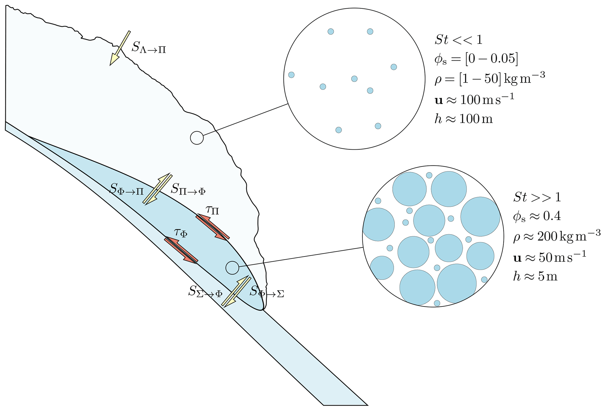
Figure 1 Conceptual sketch of a mixed-powder snow avalanche, combining an incompressible dense flow of high Stokes number with a variable density suspension cloud characterized by a small Stokes number. The avalanche growth is controlled by the erosion of the intact snow cover and the entrainment of ambient air. The layers interact through mass (yellow) and momentum fluxes (red). Characteristic scales of packing density ϕ_s, bulk density ρ, velocity u, and height h vary substantially between layers and thus require individual models.

The numerical solution and implementation are based on the finite area method (Tuković and Jasak, 2012; Rauter and Tuković, 2018) as implemented in OpenFOAM. Its modular structure and building blocks have proven to be flexible and highly valuable for physical depth-integrated models. Various code parts are reused between all models and various communities, in particular the numerical solver, geometry, and data handling, as well as various code parts related to the physics of the flow, such as friction models. Besides the introduction of the new model and its capabilities, this work highlights the extendability of the basic OpenFOAM solver to complex models.

The toolchain to process the basic terrain data, all the way to the final simulation visualization, has been improved substantially since the work of Rauter et al. (2018), and many external dependencies have been removed in order to facilitate a tight integration into OpenFOAM. Consequently, this paper also provides an updated overview of the toolchain and its practical applications. In this context we will also give a revised introduction into the finite area method and the specific derivations of depth integration. The model caters to practitioners who need a simple mixed-snow avalanche model but mostly to scientists who wish for an open model and framework that can be easily modified and extended to evaluate new concepts and ideas.

The novel model is evaluated with various synthetic test cases and finally applied to two real events: the 1988 Wolfsgruben avalanche and the 2019 Eiskar avalanche.

2 Foundation and framework

2.1 Conservation equations and depth integration

The presented method fundamentally relies on balance equations, in particular, the conservation of mass and momentum for fluids. The combination of these two equations is widely known as the Navier–Stokes equations (e.g. Ferziger and Peric, 2002) and can be written as

$$\begin{array}{}\text{(2)}& {\displaystyle }& {\displaystyle \frac{\partial \mathit{\rho }}{\partial t}}+\mathbf{\nabla }\cdot \left(\mathit{\rho }\mathit{u}\right)=\mathrm{0},\text{(3)}& {\displaystyle }& {\displaystyle \frac{\partial \mathit{\rho }\mathit{u}}{\partial t}}+\mathbf{\nabla }\cdot \left(\mathit{\rho }\mathit{u}\mathit{u}\right)=\mathbf{\nabla }\cdot \mathbf{T}+\mathit{f},\end{array}$$

with the bulk density ρ and the bulk velocity u. (Note that it can also be defined for an individual phase with some modifications, see, for example, Rauter, 2021.) These flow fields are functions of time t and space $\mathit{x}=(x,y,z{)}^T$. The model Eqs. (2) and (3) describe their evolution from a known initial state $\mathit{u}\left(\mathrm{0},\mathit{x}\right)={\mathit{u}}_{\mathrm{0}}\left(\mathit{x}\right)$ and similar ρ₀(x), under the influence of boundary conditions. The divergence of the stress tensor T has the effect of diffusing momentum, and the volume force f represents additional forces, such as gravity.

Appropriate closure relations that express the stress tensor T as a function of the unknown flow fields yield a well-posed problem that can, in principle, be solved with numerical methods (Barker and Gray, 2017). However, even a well-posed problem is often not practically solvable from a computational perspective. Therefore, multiple simplifications have to be made to make problems of practical relevance accessible. Simplifications often come in the form of averaging over a certain time or over space to get rid of turbulent structures (Reynolds averaging; see, for example, Ferziger and Peric, 2002), to describe the average behaviour of multiple interpenetrating phases (phase averaging; e.g. Rauter, 2021), or to get rid of the vertical dimension (e.g. Savage and Hutter, 1989; Rauter and Tuković, 2018). The latter is referred to as depth averaging or depth integration and avoids the calculation of three-dimensional flow details. It yields mean values of, for example, density $\stackrel{\mathrm{‾}}{\mathit{\rho }}$ and velocity $\stackrel{\mathrm{‾}}{\mathit{u}}$ along the depth.

In the simplest case, where the depth integration is aligned with a spatial axis (e.g. the z axis), the problem can be reduced from three $(x,y,z)$ to two dimensions (x,y). In this case, the depth-averaged value for an arbitrary field ψ is defined as

$$\begin{array}{}\text{(4)}& {\displaystyle }\stackrel{\mathrm{‾}}{\mathit{\psi }}(x,y,t)={\displaystyle \frac{\mathrm{1}}{h}}\underset{\mathrm{0}}{\overset{h}{\int }}\mathit{\psi }(x,y,z,t)\mathrm{d}z.\end{array}$$

The newly introduced field $h(x,y,t)$ describes the flow depth, here in terms of the z coordinate of the top boundary of the integration, for a bottom boundary assumed to be aligned with z=0. The bottom and top boundaries are usually defined such that the mass flux through them is zero, meaning that they move with the vertical velocity of the flow at the respective position. The simplest example of such a model is the shallow-water equations (Barré de Saint-Venant, 1871). Defining the boundary in any other way will lead to additional source or sink terms, depending on the mass flux through the boundary (e.g. Pudasaini and Hutter, 2007). Examples would be any kind of entrainment and deposition fluxes.

Depth-integrated models are often considered synonymous with two-dimensional models. However, real avalanches and landslides travel along paths and surfaces in three-dimensional space. The three-dimensional nature of the terrain has to be reintroduced by modifying the two-dimensional model equations. Most often this is accomplished by abandoning Cartesian coordinate systems and Euclidean geometry, which was described in detail first by Savage and Hutter (1989, 1991) and extended by many others since then (e.g. Bouchut and Westdickenberg, 2004; Denlinger and Iverson, 2004; Pudasaini et al., 2005; Hergarten and Robl, 2015). This introduces various correction terms based on Christoffel formalism that are difficult to handle in complex models. In practice, simpler approximations are frequently employed (e.g. in RAMMS, see Fischer et al., 2012), leading to a disparity between theory and practical implementation. Notably, many of these developments happened in parallel and independently in the Russian avalanche dynamics community (Eglit et al., 2020).

An alternative to two-dimensional models with excessive curvature terms is the direct solution of the governing equations in three-dimensional space (Craster and Matar, 2009; Hagemeier et al., 2011; Rauter and Tuković, 2018). Depth integration is still compatible with this approach, and it can in principle be conducted in any direction pointing out of the surface. Yet in this work, depth integration is always conducted in the direction of the normal vector n^Γ to the flow surface Γ, as shown in Fig. 2. This has formally to be conducted in a surface-aligned coordinate system x^′–y^′–z^′:

$$\begin{array}{}\text{(5)}& {\displaystyle }\stackrel{\mathrm{‾}}{\mathit{\psi }}\left({\mathit{x}}_{\mathrm{b}}\right)={\displaystyle \frac{\mathrm{1}}{h}}\underset{\mathrm{0}}{\overset{h}{\int }}\det \left(\mathbf{J}\right)\mathit{\psi }\left({\mathit{x}}^{\prime },t\right)\mathrm{d}{z}^{\prime }\approx {\displaystyle \frac{\mathrm{1}}{h}}\underset{\mathrm{0}}{\overset{h}{\int }}\mathit{\psi }\left({\mathit{x}}^{\prime },t\right)\mathrm{d}{z}^{\prime }.\end{array}$$

The Jacobian matrix J, representing the transformation $\partial {\mathit{x}}^{\prime }/\partial \mathit{x}$, and its determinant det(J) take into account the curvature of the surface and its influence on the volume in a differential volume element of the flow (Bouchut et al., 2003). This effect is of the order of $h/R$ (Bouchut et al., 2003) with the mean curvature radius R and thus is small for mildly curved surfaces (R is large in comparison to the flow height h). As in most other models, the influence of the curvature on depth integration is ignored in this work.

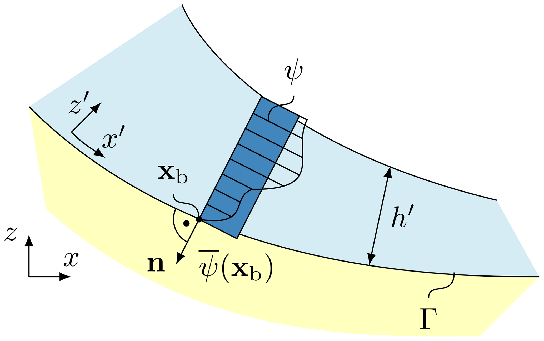
Figure 2 Depth integration reduces the full three-dimensional flow field ψ (dashed area) to an average flow field $\stackrel{\mathrm{‾}}{\mathit{\psi }}$ (blue-filled area), which is assigned to a point x_b∈Γ.

2.2 Surface partial differential equations

Depth integration in terms of Eq. (5) projects all three-dimensional flow fields on the surface Γ they are constrained by. The conservation equations can then be expressed as surface partial differential equations (SPDEs) that are defined on the surface Γ and include derivatives of various fields along it (Rauter and Tuković, 2018). These derivatives emerge from depth-integrating the nabla operator ∇ present in the Navier–Stokes equations formulated in a three-dimensional Cartesian reference frame. The presented framework differs from the classic approach of handling derivatives in two respects. Both are described in the following.

Depth integration has different effects on derivatives taken along the surface compared to those taken normal to the surface. While derivatives normal to the surface either vanish or appear as local source terms, derivatives along the surface remain in the system. A very common approach is to write the surface-aligned derivative as a two-dimensional derivative in local coordinates (e.g. in terms of $\partial x^{\prime }$, $\partial y^{\prime }$; Savage and Hutter, 1989). In the present framework, however, we express all entities in global Cartesian coordinates. For diffusive processes, this procedure gives rise to the Laplace–Beltrami operator (Dziuk and Elliott, 2013). However, this technique can also be adopted to other differential operators present in the system. The respective surface gradient and divergence operators ∇^Γ can be readily calculated in the numerical framework; see Sect. 2.3.

The depth integration of derivatives is then conducted in analogy to ordinary fields (see Eq. 5), in the surface aligned coordinate system x^′–y^′–z^′:

$$\begin{array}{ll}{\displaystyle }\stackrel{\mathrm{‾}}{\mathbf{\nabla }\mathit{\psi }}\left({\mathit{x}}_{\mathrm{b}}\right)& {\displaystyle }={\displaystyle \frac{\mathrm{1}}{h}}\underset{\mathrm{0}}{\overset{h}{\int }}\det \left(\mathbf{J}\right){\mathbf{\nabla }}^{\prime }\mathit{\psi }\left({\mathit{x}}^{\prime }\right)\mathrm{d}{z}^{\prime }\approx {\displaystyle \frac{\mathrm{1}}{h}}\underset{\mathrm{0}}{\overset{h}{\int }}{\mathbf{\nabla }}^{\prime }\mathit{\psi }\left({\mathit{x}}^{\prime }\right)\mathrm{d}{z}^{\prime }\\ {\displaystyle }& {\displaystyle }={\displaystyle \frac{\mathrm{1}}{h}}\underset{\mathrm{0}}{\overset{h}{\int }}\left({\mathbf{\nabla }}^{\mathrm{\Gamma }}\mathit{\psi }\left({\mathit{x}}^{\prime }\right)+{\displaystyle \frac{\partial }{\partial z^{\prime }}}\mathit{\psi }\left({\mathit{x}}^{\prime }\right){\mathit{e}}_z^{\prime }\right)\mathrm{d}{z}^{\prime }\\ {\displaystyle }& {\displaystyle }={\displaystyle \frac{\mathrm{1}}{h}}\underset{\mathrm{0}}{\overset{h}{\int }}{\mathbf{\nabla }}^{\mathrm{\Gamma }}\mathit{\psi }\left({\mathit{x}}^{\prime }\right)\mathrm{d}{z}^{\prime }+{\displaystyle \frac{\mathrm{1}}{h}}\underset{\mathrm{0}}{\overset{h}{\int }}{\displaystyle \frac{\partial }{\partial z^{\prime }}}\mathit{\psi }\left({\mathit{x}}^{\prime }\right)\mathrm{d}{z}^{\prime }{\mathit{e}}_z^{\prime }\\ {\displaystyle }& {\displaystyle }=\underset{\mathrm{0}}{\overset{h}{\int }}{\displaystyle \frac{{\mathbf{\nabla }}^{\mathrm{\Gamma }}\mathit{\psi }\left({\mathit{x}}^{\prime }\right)}{h}}\mathrm{d}{z}^{\prime }+{\displaystyle \frac{\mathit{\psi }\left({\mathit{x}}_{\mathrm{t}}\right)-\mathit{\psi }\left({\mathit{x}}_{\mathrm{b}}\right)}{h}}{\mathit{n}}^{\mathrm{\Gamma }}\\ \text{(6)}& {\displaystyle }& {\displaystyle }={\mathbf{\nabla }}^{\mathrm{\Gamma }}\stackrel{\mathrm{‾}}{\mathit{\psi }}\left({\mathit{x}}_{\mathrm{b}}\right)+{\displaystyle \frac{\mathit{\psi }\left({\mathit{x}}_{\mathrm{t}}\right)-\mathit{\psi }\left({\mathit{x}}_{\mathrm{b}}\right)}{h}}{\mathit{n}}^{\mathrm{\Gamma }},\end{array}$$

where x_b is a point on the bottom of the flow (and thus the flow surface Γ) and x_t the corresponding point on the free surface of the flow. The second term on the right-hand side of Eq. (6) represents an additional sink or source term, which arises if ψ is not zero at the bottom, x_b, or the top of the flow, x_t, such as due to entrainment or basal friction.

Further, our approach does not follow, for example, Savage and Hutter (1989) in separating the z component (determining, for example the pressure) from the x and y component (determining, for example, the velocity) in vectorial type balance laws such as the momentum equation. This would not be possible as our coordinate system is not aligned with the surface. We rather project the full three-dimensional equation onto the surface and the normal vector. The surface tangential projection of the surface gradient of a scalar is hence given by

$$\begin{array}{}\text{(7)}& {\displaystyle }{\mathbf{\nabla }}_{\mathrm{s}}^{\mathrm{\Gamma }}\mathit{\psi }={\mathbf{\nabla }}^{\mathrm{\Gamma }}\mathit{\psi }\cdot \left(\mathbf{I}-{\mathit{n}}^{\mathrm{\Gamma }}{\mathit{n}}^{\mathrm{\Gamma }}\right)\end{array}$$

and the surface normal projection as

$$\begin{array}{}\text{(8)}& {\displaystyle }{\mathbf{\nabla }}_{\mathrm{n}}^{\mathrm{\Gamma }}\mathit{\psi }={\mathbf{\nabla }}^{\mathrm{\Gamma }}\mathit{\psi }\cdot \left({\mathit{n}}^{\mathrm{\Gamma }}{\mathit{n}}^{\mathrm{\Gamma }}\right)\end{array}$$

and similar for vectors and divergence operators. The benefit of this approach is that the framework operates entirely in global Cartesian coordinates; thus, similar to an inertial frame, no fictitious centrifugal forces have to be considered. It follows that leading-order curvature effects are considered in the model by design, without explicitly expressing the curvature (Rauter and Tuković, 2018). For higher-order curvature effects, det(J) needs to be preserved during depth integration (Bouchut and Westdickenberg, 2004).

With these building blocks and some knowledge on how to transform one-dimensional shallow-flow models (e.g. Savage and Hutter, 1989; Parker et al., 1986), it is possible to extend nearly arbitrary depth-integrated flow models to complex terrain. In particular, ordinary depth-integrated flow models represent the surface–tangential momentum conservation equation and the flow depth equation. The two-dimensional ∇ operators have to be replaced with the surface–tangential ${\mathbf{\nabla }}_{\mathrm{s}}^{\mathrm{\Gamma }}$ operators. The surface–normal momentum conservation equation can be applied to replace the usually simplified expression for the basal pressure.

2.3 Finite area method

Partial differential equations, as well as their SPDE counterparts, are rarely solvable in an analytical sense, especially practical problems that represent real-world situations. Therefore, we rely on numerical approximations of SPDEs and the finite area method. This method is a variation of the finite volume method (see Ferziger and Peric, 2002; Jasak, 1996; Moukalled et al., 2016, for details) in N+1 dimensions, where N is the dimension of the control volumes. This means that for two-dimensional control volumes (i.e. surfaces), vectorial entities, such as normal vectors, velocities, and fluxes, will be three-dimensional. Similar to the conventional finite volume method, the Gaussian surface theorem (Tuković and Jasak, 2012) is applied and discretized by simplifying a control surface S as a flat, convex polygon S_i, as shown in Fig. 3. The expressions for the differential operators follow as

$$\begin{array}{}\text{(9)}& {\displaystyle }{\mathbf{\nabla }}^{\mathrm{\Gamma }}\mathit{\psi }={\displaystyle \frac{\mathrm{1}}{S}}\underset{\partial S}{\oint }{\mathit{m}}^{\mathrm{\Gamma }}\mathit{\psi }\mathrm{d}L\approx {\displaystyle \frac{\mathrm{1}}{S_i}}\sum {\mathit{\psi }}_{\mathrm{e}}{\mathit{m}}_{\mathrm{e}}{L}_{\mathrm{e}}\end{array}$$

and

$$\begin{array}{}\text{(10)}& {\displaystyle }{\mathbf{\nabla }}^{\mathrm{\Gamma }}\cdot \mathit{\psi }={\displaystyle \frac{\mathrm{1}}{S}}\underset{\partial S}{\oint }{\mathit{m}}^{\mathrm{\Gamma }}\cdot \mathit{\psi }\mathrm{d}L\approx {\displaystyle \frac{\mathrm{1}}{S_i}}\sum {\mathit{\psi }}_{\mathrm{e}}\cdot {\mathit{m}}_{\mathrm{e}}{L}_{\mathrm{e}}.\end{array}$$

Index e refers to a discrete number of straight edges that form the polygon with surface S_i. ψ_e is the average value of the field ψ on the edge e, L_e its length, and m_e is the Γ–tangential and edge-normal outward-pointing vector. S_i, L_e, and m_e are purely geometrical properties that are defined during mesh generation. Values of fields on edges ψ_e, on the other hand, are interpolated from values of edge-adjacent cells, ψ_P and ψ_N. This introduces flux transport across cells and represents the flow of mass or information from one cell to neighbouring ones. The fluxes can then be associated in a linear system of equations that is solved with a suitable method.

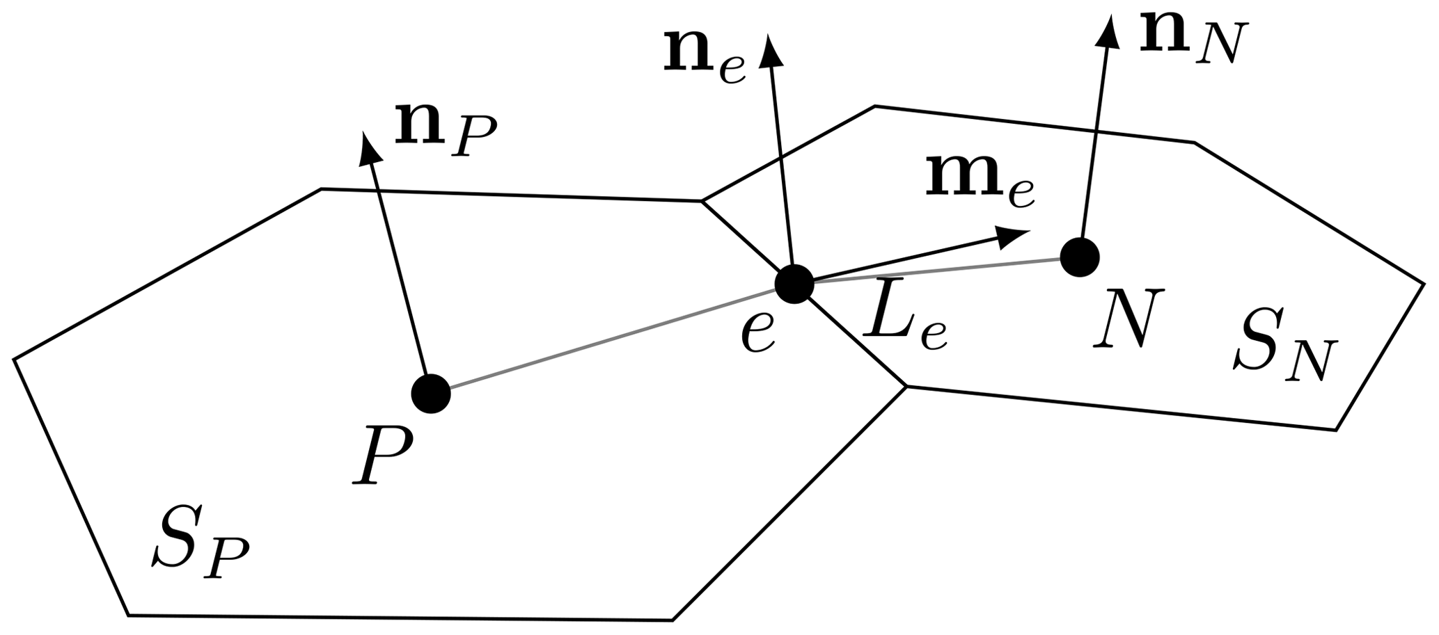
Figure 3 A finite area cell P and its neighbour N, used to calculate the approximation of surface derivatives in terms of the Gaussian surface theorem, integrating fluxes through cell edges e with length L_e and outward-pointing vector m_e.

Discretization of non-gradient terms (e.g. the temporal derivative or any source term) is done in complete analogy to the finite volume method and obtained from integration over the control surface S_i. For details we refer to the large amount of excellent literature on the finite volume method (Ferziger and Peric, 2002; Jasak, 1996; Moukalled et al., 2016; LeVeque, 2002).

3 Dense-flow model

The dense-flow model describes the flow of incompressible material with density ρ_Φ (see Fig. 1). In the case of a granular mass flow, the density follows from the grain density ρ_g and the volumetric packing density ϕ_Φ as

$$\begin{array}{}\text{(11)}& {\displaystyle }{\mathit{\rho }}_{\mathrm{\Phi }}={\mathit{\varphi }}_{\mathrm{\Phi }}{\mathit{\rho }}_{\mathrm{g}}.\end{array}$$

However, fluids can be simulated with this model as well, in which case ρ_Φ is the intrinsic density of the fluid. The depth-integrated mass and momentum conservation equations follow as

$$\begin{array}{}\text{(12)}& {\displaystyle \frac{\partial h_{\mathrm{\Phi }}}{\partial t}}+{\mathbf{\nabla }}^{\mathrm{\Gamma }}\cdot \left(h_{\mathrm{\Phi }}{\stackrel{\mathrm{‾}}{\mathit{u}}}_{\mathrm{\Phi }}\right)={\displaystyle \frac{S_{\mathrm{\Phi }}^{\mathit{\varphi }}}{{\mathit{\varphi }}_{\mathrm{\Phi }}}},\text{(13)}& {\displaystyle }\begin{array}{rl}& {\displaystyle \frac{\partial h_{\mathrm{\Phi }}{\stackrel{\mathrm{‾}}{\mathit{u}}}_{\mathrm{\Phi }}}{\partial t}}+{\mathit{\xi }}_{\mathrm{\Phi }}{\mathbf{\nabla }}_{\mathrm{s}}^{\mathrm{\Gamma }}\cdot \left(h_{\mathrm{\Phi }}{\stackrel{\mathrm{‾}}{\mathit{u}}}_{\mathrm{\Phi }}{\stackrel{\mathrm{‾}}{\mathit{u}}}_{\mathrm{\Phi }}\right)=-{\displaystyle \frac{{\mathit{\tau }}_{\mathrm{\Phi }}}{{\mathit{\rho }}_{\mathrm{\Phi }}}}+h_{\mathrm{\Phi }}{\mathit{g}}_{\mathrm{s}}\\ & -{\displaystyle \frac{\mathrm{1}}{\mathrm{2}{\mathit{\rho }}_{\mathrm{\Phi }}}}{\mathbf{\nabla }}_{\mathrm{s}}^{\mathrm{\Gamma }}\left(h_{\mathrm{\Phi }}{p}_{\mathrm{\Phi }}\right)+{\displaystyle \frac{S_{\mathrm{\Phi }}^u}{{\mathit{\rho }}_{\mathrm{\Phi }}}},\end{array}\text{(14)}& {\displaystyle }\begin{array}{rl}& {\mathit{\xi }}_{\mathrm{\Phi }}{\mathbf{\nabla }}_{\mathrm{n}}^{\mathrm{\Gamma }}\cdot \left(h_{\mathrm{\Phi }}{\stackrel{\mathrm{‾}}{\mathit{u}}}_{\mathrm{\Phi }}{\stackrel{\mathrm{‾}}{\mathit{u}}}_{\mathrm{\Phi }}\right)=h_{\mathrm{\Phi }}{\mathit{g}}_{\mathrm{n}}-{\displaystyle \frac{\mathrm{1}}{\mathrm{2}{\mathit{\rho }}_{\mathrm{\Phi }}}}{\mathbf{\nabla }}_{\mathrm{n}}^{\mathrm{\Gamma }}\left(h_{\mathrm{\Phi }}{p}_{\mathrm{\Phi }}\right)\\ & -{\displaystyle \frac{\mathrm{1}}{{\mathit{\rho }}_{\mathrm{\Phi }}}}{\mathit{n}}^{\mathrm{\Gamma }}{p}_{\mathrm{\Phi }}.\end{array}\end{array}$$

The unknown flow fields are the flow depth h_Φ, the depth-integrated velocity ${\stackrel{\mathrm{‾}}{\mathit{u}}}_{\mathrm{\Phi }}$, and the basal pressure p_Φ. The gravitational acceleration is represented by its surface–tangential projection ${\mathit{g}}_{\mathrm{s}}=\left(\mathbf{I}-{\mathit{n}}^{\mathrm{\Gamma }}{\mathit{n}}^{\mathrm{\Gamma }}\right)\mathit{g}$ and its surface-normal projection g_n=(n^Γ n^Γ)g. Equation (14) represents the surface-normal component of the momentum conservation equation and yields the basal pressure p_Φ.

The shape factor ξ_Φ partially compensates for errors introduced by switching integration and multiplication, namely ${\mathit{\xi }}_{\mathrm{\Phi }}{\stackrel{\mathrm{‾}}{\mathit{u}}}_{\mathrm{\Phi }}{\stackrel{\mathrm{‾}}{\mathit{u}}}_{\mathrm{\Phi }}=\stackrel{\mathrm{‾}}{{\mathit{u}}_{\mathrm{\Phi }}{\mathit{u}}_{\mathrm{\Phi }}}$. It depends on the velocity profile and as such on the constitutive model and the state of the flow. It is usually neglected or set to a theoretical and constant value, derived, for example, from the Bagnold (1954) velocity profile (${\mathit{\xi }}_{\mathrm{\Phi }}=\mathrm{5}/\mathrm{4}$).

3.1 Friction in the dense-flow model

The term τ_Φ represents the depth-integrated divergence of the shear stress tensor and thus the constitutive model of the flowing mass. Assuming that the top boundary is stress-free and that surface–tangential derivatives of the deviatoric stress tensor are small, the only remaining entity is the basal friction. In this work, we will use the friction model presented by Rauter et al. (2016), which is closely related to the widely used Voellmy (1955) friction model. It is given as

$$\begin{array}{}\text{(15)}& {\displaystyle }{\mathit{\tau }}_{\mathrm{\Phi }}=\left(\mathit{\mu }{p}_{\mathrm{\Phi }}+{\displaystyle \frac{{\mathit{\rho }}_{\mathrm{\Phi }}\left|\mathit{g}\right|}{\mathit{\chi }{h}_{\mathrm{\Phi }}^{\mathrm{2}}}}|{\stackrel{\mathrm{‾}}{\mathit{u}}}_{\mathrm{\Phi }}{|}^{\mathrm{2}}\right){\displaystyle \frac{{\stackrel{\mathrm{‾}}{\mathit{u}}}_{\mathrm{\Phi }}}{\left|{\stackrel{\mathrm{‾}}{\mathit{u}}}_{\mathrm{\Phi }}\right|}},\end{array}$$

with dry friction coefficient μ and turbulent friction coefficient χ. A wide range of alternative friction models can be found in the literature, and a number of them are implemented in the presented software.

3.2 Entrainment and deposition in the dense-flow model

$S_{\mathrm{\Phi }}^{\mathit{\varphi }}$ represents the sum of all volumetric source and sink terms of grains (e.g. erosion and entrainment of additional mass or its deposition), and $S_{\mathrm{\Phi }}^u$ represents its associated momentum. Dividing by the packing density in Eq. (12) simplifies handling of density changes in the different flow regimes. In the simplest case (e.g. laboratory experiments on a non-erodible bed), the source and sink terms are zero.

For snow avalanches and many other realistic gravitational mass flows, entrainment of erodible material along the avalanche path plays an important role. A popular entrainment model can be derived by comparing the dissipated energy in the mass flow with the energy required to mobilize the static material (Fischer et al., 2015):

$$\begin{array}{}\text{(16)}& {\displaystyle }{S}_{\mathrm{\Sigma }\to \mathrm{\Phi }}^{\mathit{\varphi }}={\displaystyle \frac{{\mathit{\tau }}_{\mathrm{\Phi }}\cdot {\stackrel{\mathrm{‾}}{\mathit{u}}}_{\mathrm{\Phi }}}{{\mathit{\rho }}_{\mathrm{\Phi }}{e}_{\mathrm{b}}}}{\mathit{\varphi }}_{\mathrm{\Phi }},\end{array}$$

with the specific erosion energy e_b as the single parameter. Here it is assumed that the packing density of the static layer is the same as in the dense flow ϕ_Φ.

Rauter and Köhler (2020) presented an extension to account for the deposition of flowing material, $S_{\mathrm{\Phi }\to \mathrm{\Sigma }}^{\mathit{\varphi }}$. This aspect is neglected in this work, and the flow height of the last time step is assumed to be the final deposition of the model.

The total flux term between the static layer and the flowing avalanche is determined as the difference between entrainment and deposition:

$$\begin{array}{}\text{(17)}& {\displaystyle }{S}_{\mathrm{\Phi }}^{\mathit{\varphi }}=S_{\mathrm{\Sigma }\to \mathrm{\Phi }}^{\mathit{\varphi }}-S_{\mathrm{\Phi }\to \mathrm{\Sigma }}^{\mathit{\varphi }}.\end{array}$$

The related momentum source and sink terms are zero in the case of single layer flows, as both erodible material and deposited material are static.

The height (in surface-normal direction) of the static material on the topography can be tracked with an additional evolution equation:

$$\begin{array}{}\text{(18)}& {\displaystyle }{\displaystyle \frac{\partial h_{\mathrm{\Sigma }}}{\partial t}}={\displaystyle \frac{S_{\mathrm{\Sigma }}^{\mathit{\varphi }}}{{\mathit{\varphi }}_{\mathrm{\Phi }}}},\end{array}$$

with

$$\begin{array}{}\text{(19)}& {\displaystyle }{S}_{\mathrm{\Sigma }}^{\mathit{\varphi }}=S_{\mathrm{\Phi }\to \mathrm{\Sigma }}^{\mathit{\varphi }}-S_{\mathrm{\Sigma }\to \mathrm{\Phi }}^{\mathit{\varphi }},\end{array}$$

again under the assumption that the static layer has the same packing density as the flowing avalanche ϕ_Φ. Tracking the thickness of the static layer allows the limitation of the available entrainable material; hence we are able to turn off entrainment if the erodible layer is depleted.

4 Suspension flow model

The suspension flow model describes the flow of a dynamic mixture of a granular material of density ρ_g and the surrounding fluid of density ρ_c. It corresponds, to some degree, to a depth integration of the compressible model of Rauter (2021). The mixture density follows as

$$\begin{array}{}\text{(20)}& {\displaystyle }{\mathit{\rho }}_{\mathrm{\Pi }}={\mathit{\varphi }}_{\mathrm{\Pi }}{\mathit{\rho }}_{\mathrm{g}}+\left(\mathrm{1}-{\mathit{\varphi }}_{\mathrm{\Pi }}\right){\mathit{\rho }}_{\mathrm{c}},\end{array}$$

with the variable packing density or phase fraction ϕ_Π. Introducing the buoyant density ratio,

$$\begin{array}{}\text{(21)}& {\displaystyle }r={\displaystyle \frac{{\mathit{\rho }}_{\mathrm{g}}-{\mathit{\rho }}_{\mathrm{c}}}{{\mathit{\rho }}_{\mathrm{c}}}}.\end{array}$$

The mixture density can be expressed as

$$\begin{array}{}\text{(22)}& {\displaystyle }{\mathit{\rho }}_{\mathrm{\Pi }}={\mathit{\rho }}_{\mathrm{c}}\left(\mathrm{1}+{\mathit{\varphi }}_{\mathrm{\Pi }}r\right).\end{array}$$

The Boussinesq approximation, an often applied simplification (e.g. Parker et al., 1986), implies that ${\mathit{\varphi }}_{\mathrm{\Pi }}⪅{\mathrm{10}}^{-\mathrm{2}}$ and r≈1 and thus ρ_Π≈ρ_c. This is reasonable if ρ_g and ρ_c are at least similar in order of magnitude (e.g. sand in water). However, this does not hold for snow avalanches, i.e. mixtures of grains or ice (ρ_g≈1000 kg m⁻³) with air (ρ_c≈1 kg m⁻³). Thus, we will omit this assumption and consider the dynamic density as given by Eq. (22) in all terms.

Due to the variable mixture, there will be two phases that have to be described by balance laws. In depth-averaged frameworks, this is usually handled by describing the total volume occupied by the flowing masses (grains and flowing ambient fluid) in terms of the flow depth h_Π and the volume of grains, expressed by the depth-integrated volume fraction $h_{\mathrm{\Pi }}{\stackrel{\mathrm{‾}}{\mathit{\varphi }}}_{\mathrm{\Pi }}$ (e.g. Parker et al., 1986). The phases are assumed to move with the same velocity ${\stackrel{\mathrm{‾}}{\mathit{u}}}_{\mathrm{\Pi }}$. Differences in velocity (e.g. settling of particles) are considered with empirical corrections.

The depth-integrated mass and momentum conservation equations follow as

$$\begin{array}{}\text{(23)}& {\displaystyle \frac{\partial h_{\mathrm{\Pi }}}{\partial t}}+{\mathbf{\nabla }}^{\mathrm{\Gamma }}\cdot \left(h_{\mathrm{\Pi }}{\stackrel{\mathrm{‾}}{\mathit{u}}}_{\mathrm{\Pi }}\right)=S_{\mathrm{\Pi }}^h,\text{(24)}& {\displaystyle \frac{\partial {\stackrel{\mathrm{‾}}{\mathit{\varphi }}}_{\mathrm{\Pi }}{h}_{\mathrm{\Pi }}}{\partial t}}+{\mathbf{\nabla }}^{\mathrm{\Gamma }}\cdot \left({\stackrel{\mathrm{‾}}{\mathit{\varphi }}}_{\mathrm{\Pi }}{h}_{\mathrm{\Pi }}{\stackrel{\mathrm{‾}}{\mathit{u}}}_{\mathrm{\Pi }}\right)=S_{\mathrm{\Pi }}^{\mathit{\varphi }},\text{(25)}& {\displaystyle }\begin{array}{rl}& {\displaystyle \frac{\partial \left(\mathrm{1}+r{\stackrel{\mathrm{‾}}{\mathit{\varphi }}}_{\mathrm{\Pi }}\right)h_{\mathrm{\Pi }}{\stackrel{\mathrm{‾}}{\mathit{u}}}_{\mathrm{\Pi }}}{\partial t}}+{\mathit{\xi }}_{\mathrm{\Pi }}{\mathbf{\nabla }}_{\mathrm{s}}^{\mathrm{\Gamma }}\cdot \left(\left(\mathrm{1}+r{\stackrel{\mathrm{‾}}{\mathit{\varphi }}}_{\mathrm{\Pi }}\right)h_{\mathrm{\Pi }}{\stackrel{\mathrm{‾}}{\mathit{u}}}_{\mathrm{\Pi }}{\stackrel{\mathrm{‾}}{\mathit{u}}}_{\mathrm{\Pi }}\right)\\ & =-{\displaystyle \frac{{\mathit{\tau }}_{\mathrm{\Pi }}}{{\mathit{\rho }}_{\mathrm{c}}}}+r{\stackrel{\mathrm{‾}}{\mathit{\varphi }}}_{\mathrm{\Pi }}{h}_{\mathrm{\Pi }}{\mathit{g}}_{\mathrm{s}}-{\displaystyle \frac{\mathrm{1}}{\mathrm{2}}}{\mathbf{\nabla }}_{\mathrm{s}}^{\mathrm{\Gamma }}\left(\left(\mathrm{1}+r{\stackrel{\mathrm{‾}}{\mathit{\varphi }}}_{\mathrm{\Pi }}\right)g_{\mathrm{eff}}{h}_{\mathrm{\Pi }}^{\mathrm{2}}\right)\\ & +{\displaystyle \frac{S_{\mathrm{\Pi }}^u}{{\mathit{\rho }}_{\mathrm{c}}}}.\end{array}\end{array}$$

All equations and terms are well known from the dense-flow model, except for the additional tracking of the grain fraction with Eq. (24). The unknown flow fields are the flow depth h_Π, the depth-averaged velocity ${\stackrel{\mathrm{‾}}{\mathit{u}}}_{\mathrm{\Pi }}$, and the depth-averaged phase fraction or packing density ${\stackrel{\mathrm{‾}}{\mathit{\varphi }}}_{\mathrm{\Pi }}$. Assuming $r{\stackrel{\mathrm{‾}}{\mathit{\varphi }}}_{\mathrm{\Pi }}\approx \mathrm{0}$ in all terms but the gravitational acceleration (buoyancy assumption) leads to the popular model of Parker et al. (1986). Removing the surface–tangential gravitational acceleration leads to the momentum conservation equation of Bartelt et al. (2016). The effective gravitational acceleration g_eff is the surface-normal gravitational acceleration, corrected for centripetal acceleration due to curved terrain. In terms of surface partial differential equations, it can be easily expressed as (see Appendix A)

$$\begin{array}{}\text{(26)}& {\displaystyle }{g}_{\mathrm{eff}}\approx {\mathit{n}}^{\mathrm{\Gamma }}\cdot \left(\mathit{g}-{\mathbf{\nabla }}^{\mathrm{\Gamma }}\cdot \left({\stackrel{\mathrm{‾}}{\mathit{u}}}_{\mathrm{\Pi }}{\stackrel{\mathrm{‾}}{\mathit{u}}}_{\mathrm{\Pi }}\right)\right).\end{array}$$

This expression replaces the rather complex calculation of the basal pressure in the dense-flow model. It is justified here, as the basal pressure has only a weak influence on the flow dynamics of the suspended flow. Further, this notation turns out to be convenient later, as various internal processes in the suspension flow depend on effective gravity. A particle on a streamline of the flow will approximately experience a volume force corresponding to this acceleration, and processes like the terminal settling velocity will depend on this adjusted value.

Considerable attention has to be drawn to the volumetric source and sink terms ($S_{\mathrm{\Pi }}^h$ and $S_{\mathrm{\Pi }}^{\mathit{\varphi }}$) and the associated momentum flux ($S_{\mathrm{\Pi }}^u$). These terms are responsible for the varying flow height and the depth-averaged particle volume fraction and influence the flow dynamics substantially.

4.1 Friction in the suspension flow model

Similarly as in the dense-flow model, the term τ_Π represents the depth-integrated divergence of the shear stress tensor. If the particle fraction in the suspension is low, it can be treated as a simple fluid. The simplest wall friction model can be represented with constant friction coefficient c_D (Parker et al., 1986):

$$\begin{array}{}\text{(27)}& {\displaystyle }{\mathit{\tau }}_{\mathrm{\Pi }}={\mathit{\rho }}_{\mathrm{c}}{c}_{\mathrm{D}}\left|{\stackrel{\mathrm{‾}}{\mathit{u}}}_{\mathrm{\Pi }}\right|{\stackrel{\mathrm{‾}}{\mathit{u}}}_{\mathrm{\Pi }}.\end{array}$$

However, suspension flows are inherently turbulent, and there is strong evidence that turbulence models with more complex friction relations might be required (e.g. Parker et al., 1986). Nevertheless, we will use the simple model in this work, and we should keep in mind that the wall friction coefficient c_D is an empirical parameter that might require adaption to flow conditions. Further, it is assumed that all dissipative processes, such as inter-granular friction (e.g. Boyer et al., 2011), are included in this term. Considering the accuracy and uncertainties of the problems at hand, this seems to be a reasonable compromise. Alternative approaches are the turbulence model of Parker et al. (1986), a depth integration of the Einstein viscosity model (e.g. Boyer et al., 2011), and a more complex granular rheology (Boyer et al., 2011).

4.2 Ambient fluid entrainment in the suspension flow model

The volume of the suspension flow will grow due to entrainment of ambient fluid. It is assumed (Parker et al., 1986; Turner, 1986; Ancey, 2004) that ambient fluid entrainment depends solely on the bulk Richardson number, which is given as

$$\begin{array}{}\text{(28)}& {\displaystyle }{\mathit{Ri}}_{\mathrm{\Pi }}={\displaystyle \frac{r{g}_{\mathrm{eff}}{\stackrel{\mathrm{‾}}{\mathit{\varphi }}}_{\mathrm{\Pi }}{h}_{\mathrm{\Pi }}}{{\stackrel{\mathrm{‾}}{\mathit{u}}}_{\mathrm{\Pi }}^{\mathrm{2}}}}.\end{array}$$

In contrast to, for example, Parker et al. (1986), we use the effective surface-normal acceleration g_eff instead of the constant gravitational acceleration $\left|\mathit{g}\right|$ to account for the influence of centripetal forces on particles in the flow. Adjusting the Richardson number with the centripetal acceleration leads to an increased amount of ambient fluid entrainment if the flow runs over convex terrain and to a decreased amount if the flow runs over concave terrain.

There are various models for the relation between the Richardson number and the entrainment. Parker et al. (1986) use a simple, inverse proportional approach:

$$\begin{array}{}\text{(29)}& {\displaystyle }{S}_{\mathrm{\Lambda }\to \mathrm{\Pi }}^h=\left|{\stackrel{\mathrm{‾}}{\mathit{u}}}_{\mathrm{\Pi }}\right|{\displaystyle \frac{\mathit{\alpha }}{R{i}_{\mathrm{0}}+R{i}_{\mathrm{\Pi }}}},\end{array}$$

with the parameters α=0.00153 and Ri₀=0.204.

Turner (1986) provides an alternative formulation:

$$\begin{array}{}\text{(30)}& {\displaystyle }{S}_{\mathrm{\Lambda }\to \mathrm{\Pi }}^h=\left|{\stackrel{\mathrm{‾}}{\mathit{u}}}_{\mathrm{\Pi }}\right|\left\{\begin{array}{ll}{\displaystyle \frac{R{i}_{\mathrm{0}}-R{i}_{\mathrm{\Pi }}}{{\mathit{\alpha }}_{\mathrm{1}}+{\mathit{\alpha }}_{\mathrm{2}}{\mathit{Ri}}_{\mathrm{\Pi }}}}& \text{for }R{i}_{\mathrm{\Pi }}<R{i}_{\mathrm{0}},\\ \mathrm{0}& \text{for }R{i}_{\mathrm{\Pi }}\ge R{i}_{\mathrm{0}},\end{array}\right.\end{array}$$

with the parameters Ri₀=0.8, α₁=10, and α₂=50. Various different parameters were suggested for this empirical relation (see, for example, Ancey, 2004).

Finally, Ancey (2004) suggests yet another relation in the form of an exponential function, here given in the form of Issler et al. (2018):

$$\begin{array}{}\text{(31)}& {\displaystyle }{S}_{\mathrm{\Lambda }\to \mathrm{\Pi }}^h=\left|{\stackrel{\mathrm{‾}}{\mathit{u}}}_{\mathrm{\Pi }}\right|{\mathit{\alpha }}_{\mathrm{2}}\left\{\begin{array}{ll}\exp \left(-{\mathit{\alpha }}_{\mathrm{1}}R{i}^{\mathrm{2}}\right)& \text{for }R{i}_{\mathrm{\Pi }}<\mathrm{1},\\ \exp \left(-{\mathit{\alpha }}_{\mathrm{1}}\right)/Ri& \text{for }R{i}_{\mathrm{\Pi }}\ge \mathrm{1}.\end{array}\right.\end{array}$$

The parameter α₁ is supposed to be the only free parameter, with a value of 1.6 following Issler et al. (2018); however, due to different definitions of the entrainment rate, an additional parameter α₂ is required. In order to be of similar magnitude as the other air entrainment relations, α₂ has to be roughly 0.05. All relations are shown in Fig. 4.

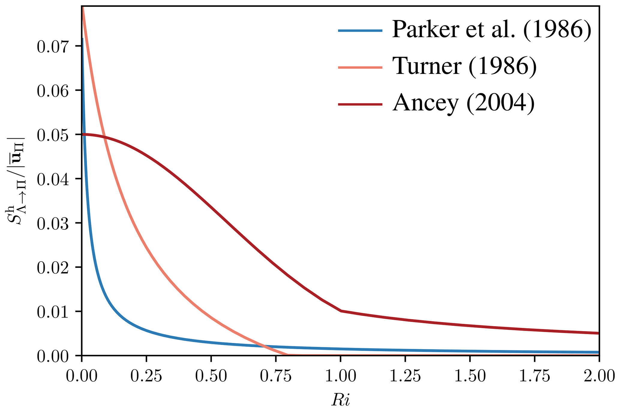
Figure 4 Comparison of the air entrainment functions, all depending solely on the Richardson number Ri.

4.3 Grain entrainment and settlement in the suspension flow model

Suspension flows are, similar to dense flows, able to erode granular material from the bed. It is, in principle, possible to use the same entrainment relations as in the dense-flow model, but specialized entrainment relations have been proposed in the literature. An example of subaquatic turbidity currents, is given by Parker et al. (1986) as

$$\begin{array}{}\text{(32)}& \begin{array}{rl}& S_{\mathrm{\Sigma }\to \mathrm{\Pi }}^{\mathit{\varphi }}=v_{\mathrm{s}}\\ & \left\{\begin{array}{ll}\mathrm{0.3}& \text{for }Z>Z_{\mathrm{m}},\\ \mathrm{3}\times {\mathrm{10}}^{-\mathrm{12}}{Z}^{\mathrm{10}}\left(\mathrm{1}-\frac{Z_{\mathrm{c}}}{Z}\right)& \text{for }{Z}_{\mathrm{c}}<Z<Z_{\mathrm{m}},\\ \mathrm{0}& \text{for }Z<Z_{\mathrm{e}},\end{array}\right.\end{array}\end{array}$$

with

$$\begin{array}{}\text{(33)}& {\displaystyle }Z{\displaystyle }={\mathit{Re}}_{\mathrm{g}}{\displaystyle \frac{\sqrt{{\mathit{\tau }}_{\mathrm{\Pi }}}}{v_{\mathrm{s}}}};\end{array}$$

the settling velocity,

$$\begin{array}{}\text{(34)}& {\displaystyle }{v}_{\mathrm{s}}{\displaystyle }={\displaystyle \frac{r{g}_{\mathrm{eff}}{d}_{\mathrm{\Pi }}^{\mathrm{2}}}{\mathrm{18}{\mathit{\nu }}_{\mathrm{c}}}};\end{array}$$

the particle Reynolds number,

$$\begin{array}{}\text{(35)}& {\displaystyle }{\mathit{Re}}_{\mathrm{g}}{\displaystyle }={\displaystyle \frac{\sqrt{r{g}_{\mathrm{eff}}{d}_{\mathrm{\Pi }}}{d}_{\mathrm{\Pi }}}{{\mathit{\nu }}_{\mathrm{c}}}};\end{array}$$

the viscosity of the ambient fluid ν_c; and two empirical parameters Z_m=13.2 and Z_c. The parameter Z_c was reported to be approximately 5. We found that a value of exactly 0.5 is required to reproduce the examples of Parker et al. (1986) in the examples shown in Sect. 7.2.

The settling of grains is given by Parker et al. (1986) as

$$\begin{array}{}\text{(36)}& {\displaystyle }{S}_{\mathrm{\Pi }\to \mathrm{\Sigma }}^{\mathit{\varphi }}=v_{\mathrm{s}}{r}_{\mathrm{0}}{\mathit{\varphi }}_{\mathrm{\Pi }},\end{array}$$

with the settling velocity as given in Eq. (34) and the factor r₀ for the bottom value of the grain concentration,

$$\begin{array}{}\text{(37)}& {\displaystyle }{r}_{\mathrm{0}}=\mathrm{1}+\mathrm{31.5}{\left(\sqrt{{\displaystyle \frac{{\mathit{\tau }}_{\mathrm{\Pi }}}{{\mathit{\rho }}_{\mathrm{c}}}}}{\displaystyle \frac{\mathrm{1}}{v_{\mathrm{s}}}}\right)}^{-\mathrm{1.46}}.\end{array}$$

As before, the total flux term follows as the difference between entrainment and deposition:

$$\begin{array}{}\text{(38)}& {\displaystyle }{S}_{\mathrm{\Pi }}^{\mathit{\varphi }}=S_{\mathrm{\Sigma }\to \mathrm{\Pi }}^{\mathit{\varphi }}-S_{\mathrm{\Pi }\to \mathrm{\Sigma }}^{\mathit{\varphi }}.\end{array}$$

The momentum flux into the suspension due to ambient fluid and grain entrainment is zero. The volume occupied by entrained and deposited grains and the respective flux term in the evolution equation of the flow height h_Π are neglected at this point.

5 Two-layer granular flow model

Granular mass flows can show different regimes, especially in terms of the Stokes number. Sampl and Zwinger (2004) and others (Jóhannesson et al., 2009) describe three regimes: the dense flow, transition or re-suspension, and powder snow layer. Sovilla et al. (2015) recognize five regions in mixed-snow avalanches, and Köhler et al. (2018) identified seven regimes. Here we aim to represent the two limit cases of dense flow and suspension in a single model, similar to Bartelt et al. (2016). It is assumed that these regimes are described in appropriate accuracy either by the Savage and Hutter (1989, 1991) model (Eqs. 12 to 14) or the Parker et al. (1986) model (Eqs. 23 to 25). The layers will communicate with mass fluxes S^ϕ and S^h and momentum fluxes S^u. In particular, the fluxes of grains are (see also Fig. 1) for the static layer,

$$\begin{array}{}\text{(39)}& {\displaystyle }{S}_{\mathrm{\Sigma }}^{\mathit{\varphi }}=S_{\mathrm{\Phi }\to \mathrm{\Sigma }}^{\mathit{\varphi }}-S_{\mathrm{\Sigma }\to \mathrm{\Phi }}^{\mathit{\varphi }},\end{array}$$

for the dense-flow layer,

$$\begin{array}{}\text{(40)}& {\displaystyle }{S}_{\mathrm{\Phi }}^{\mathit{\varphi }}=S_{\mathrm{\Sigma }\to \mathrm{\Phi }}^{\mathit{\varphi }}-S_{\mathrm{\Phi }\to \mathrm{\Sigma }}^{\mathit{\varphi }}+S_{\mathrm{\Pi }\to \mathrm{\Phi }}^{\mathit{\varphi }}-S_{\mathrm{\Phi }\to \mathrm{\Pi }}^{\mathit{\varphi }},\end{array}$$

and for the suspension layer

$$\begin{array}{}\text{(41)}& {\displaystyle }{S}_{\mathrm{\Pi }}^{\mathit{\varphi }}=S_{\mathrm{\Phi }\to \mathrm{\Pi }}^{\mathit{\varphi }}-S_{\mathrm{\Pi }\to \mathrm{\Phi }}^{\mathit{\varphi }}.\end{array}$$

Entrainment by the suspension layer is assumed to be negligibly small in comparison to the overall mass fluxes and thus is not explicitly accounted for in the simulations. The term $S_{\mathrm{\Phi }\to \mathrm{\Pi }}^{\mathit{\varphi }}$ describes the upward mass flux from the dense flow to the suspension flow. It is the remaining term to be specified in the following (see Sect. 5.1). The flux in the opposite direction $S_{\mathrm{\Pi }\to \mathrm{\Phi }}^{\mathit{\varphi }}$ is assumed to be equal to the settling flux of the suspension layer $S_{\mathrm{\Pi }\to \mathrm{\Sigma }}^{\mathit{\varphi }}$; i.e. the deposition from the suspension is redirected to the dense core and further to the static layer from there, if the deposition model of the dense-flow model is active. The corresponding momentum fluxes for the dense-flow layer and the suspension layer are

$$\begin{array}{}\text{(42)}& {\displaystyle }{\mathbf{S}}_{\mathrm{\Phi }}^u=-{\mathbf{S}}_{\mathrm{\Pi }}^u={\stackrel{\mathrm{‾}}{\mathit{u}}}_{\mathrm{\Pi }}{S}_{\mathrm{\Pi }\to \mathrm{\Phi }}^{\mathit{\varphi }}-{\mathit{\xi }}_{\mathrm{t}\mathrm{\Phi }}{\stackrel{\mathrm{‾}}{\mathit{u}}}_{\mathrm{\Phi }}{S}_{\mathrm{\Phi }\to \mathrm{\Pi }}^{\mathit{\varphi }},\end{array}$$

accounting for the momentum that is transferred together with grains between moving layers. The shape factor ξ_t takes into account that the velocity at the top boundary of the avalanche, where particles are tossed into the suspension layer, is higher than the depth-integrated velocity. It is related to the previously shown shape factor and can similarly be calculated on the basis of, for example, the Bagnold (1954) velocity profile as $\mathrm{5}/\mathrm{3}$. The particles that fall from the suspension layer onto the dense-flow layer, $S_{\mathrm{\Pi }\to \mathrm{\Phi }}^{\mathit{\varphi }}$, are assumed to carry the velocity of the suspension layer. While the exact form of this flux is not important, it is vital to remove momentum together with mass, so as to not increase the velocity of the remaining mass to potentially very high values. The momentum fluxes to and from the static layer are zero due to the respective velocity at the interface.

Further we have to account for the volume of fluid that is pushed into the suspension layer with particles. Assuming that particles enter at a packing density of ϕ_0Π, we have to add a source term of the form

$$\begin{array}{}\text{(43)}& {\displaystyle }{S}_{\mathrm{\Phi }\to \mathrm{\Pi }}^h={\displaystyle \frac{S_{\mathrm{\Phi }\to \mathrm{\Pi }}^{\mathit{\varphi }}}{{\mathit{\varphi }}_{\mathrm{0}\mathrm{\Pi }}}}.\end{array}$$

The value ϕ_0Π is set to the phase fraction of the dense core in this work. This avoids unreasonably high grain fractions if a suspension flow is initiated by a dense-flow avalanche.

In addition to the particle-borne momentum fluxes, we need to consider the shear stress at the interface. This relation is chosen to be identical to the basal shear stress of the suspension layer, τ_Π; however, it is no longer proportional to the velocity of the suspension layer but to the relative velocity between the dense-flow and the suspension layer:

$$\begin{array}{}\text{(44)}& {\displaystyle }{\mathit{\tau }}_{\mathrm{\Pi }}={\mathit{\rho }}_{\mathrm{c}}{c}_{\mathrm{D}}|{\stackrel{\mathrm{‾}}{\mathit{u}}}_{\mathrm{\Pi }}-{\stackrel{\mathrm{‾}}{\mathit{u}}}_{\mathrm{\Phi }}|\left({\stackrel{\mathrm{‾}}{\mathit{u}}}_{\mathrm{\Pi }}-{\stackrel{\mathrm{‾}}{\mathit{u}}}_{\mathrm{\Phi }}\right).\end{array}$$

In areas where the suspension layer detaches from the dense flow, the dense-flow velocity is assumed to be zero, and the model collapses to the friction model of the ordinary suspension model. An equal but opposite stress term to τ_Π should be applied to the dense core to account for the friction of the top surface of the dense core. However, it is assumed that this stress is already included in the empirical formulation and parameterization of τ_Φ, because the top surface friction is also present in pure dense-snow avalanches with a stationary or moving air layer above it. The ambient fluid entrainment of the suspension layer stays unchanged.

The mass flux $S_{\mathrm{\Phi }\to \mathrm{\Pi }}^{\mathit{\varphi }}$ feeds the suspension layer from the dense core; the associated momentum flux, in combination with the shape factor, propels the suspension flow forwards. This is assumed to be the mayor genesis mechanism for the suspension cloud, as in most other avalanche models.

5.1 Cross-layer coupling

All fluxes of the two-layer model are described relatively well in the literature (see sections above), except for the mass flux from the dense-flow layer to the suspension layer, $S_{\mathrm{\Phi }\to \mathrm{\Pi }}^{\mathit{\varphi }}$, for which only few suggestions can be found (Eglit, 1998; Issler, 1998; Sampl and Zwinger, 2004; Bartelt et al., 2016). Existing relations do not conceptually fit into the presented framework, either due to missing granular mechanics (Eglit, 1998; Issler, 1998; Sampl and Zwinger, 2004) or due to their dependence on a specific dense-flow model (Bartelt et al., 2016). For the purpose of introducing this framework, we choose a simple relation, based on local flow fields of the dense flow.

We assume that the dense flow is composed of small and large particles with diameters d_Π and d_Φ, respectively. Uptake of particles into the suspension layer requires small particles to be made available by the dense layer that mostly consists of large particles (Bartelt et al., 2016) and the capability of the suspension layer to keep them suspended. The latter is already implemented into the model in the form of the settling model of the suspension flow $S_{\mathrm{\Pi }\to \mathrm{\Phi }}^{\mathit{\varphi }}$. This term depends on the particle Reynolds number Re_g, which is similar to the Stokes number and a good indicator of the flow regime.

The first step, making small particles available to the suspension, is assumed to be triggered by a fluidized flow that expands in volume, sucks in air, and increases the distance between particles. There are various hints on how this expression should look. At first it is useful to look at dimensionless properties in the dense flow. Besides the non-dimensional volumetric mass flux $S_{\mathrm{\Phi }\to \mathrm{\Pi }}^{\mathit{\varphi }}/\left|{\stackrel{\mathrm{‾}}{\mathit{u}}}_{\mathrm{\Phi }}\right|$, these are the friction coefficient ${\mathit{\mu }}_{\mathrm{\Phi }}=\left|{\mathit{\tau }}_{\mathrm{\Phi }}\right|/p_{\mathrm{\Phi }}$, the packing density ϕ_Φ, and the inertial number (Forterre and Pouliquen, 2008; Rauter, 2021):

$$\begin{array}{}\text{(45)}& {\displaystyle }{I}_{\mathrm{\Phi }}={\displaystyle \frac{d_{\mathrm{\Phi }}{\dot{\mathit{\gamma }}}_{\mathrm{\Phi }}}{\sqrt{p_{\mathrm{\Phi }}/{\mathit{\rho }}_{\mathrm{g}}}}},\end{array}$$

with the shear rate at the bottom of the dense flow, which is assumed to follow Bagnold (1954):

$$\begin{array}{}\text{(46)}& {\displaystyle }{\dot{\mathit{\gamma }}}_{\mathrm{\Phi }}={\displaystyle \frac{\mathrm{4}}{\mathrm{3}}}{\displaystyle \frac{\left|{\stackrel{\mathrm{‾}}{\mathit{u}}}_{\mathrm{\Phi }}\right|}{h_{\mathrm{\Phi }}}}.\end{array}$$

It is well established that μ_Φ and ϕ_Φ can be expressed as a function of only the inertial number I_Φ, and it is reasonable to assume that fluidization can be described the same way. This is further emphasized by the linear relationship between the packing density and the inertial number in the dense-flow regime (Forterre and Pouliquen, 2008). Finally, Rauter et al. (2016) found a specific relation between the shear rate ${\dot{\mathit{\gamma }}}_{\mathrm{\Phi }}$ and the pressure p_Φ in a granular kinetic theory model (Vescovi et al., 2013) at the point where fluidization suddenly occurs:

$$\begin{array}{}\text{(47)}& {\displaystyle \frac{{\dot{\mathit{\gamma }}}_{\mathrm{\Phi }}}{p_{\mathrm{\Phi }}^{\mathrm{0.37}}}}=\text{const.}\end{array}$$

Comparing this relation to the expression for the inertial number, one can observe a striking resemblance; solely the exponent of the pressure is slightly lower in the relation of Rauter et al. (2016). This strongly indicates that the mass flux from the dense flow to the suspension can be expressed as a function of the inertial number only, starting at a minimum value I₀ and growing with a specified rate s_f from thereon:

$$\begin{array}{}\text{(48)}& {\displaystyle \frac{S_{\mathrm{\Phi }\to \mathrm{\Pi }}^{\mathit{\varphi }}}{\left|{\stackrel{\mathrm{‾}}{\mathit{u}}}_{\mathrm{\Phi }}\right|}}\left(I_{\mathrm{\Phi }}\right)=max\left(I_{\mathrm{\Phi }}-I_{\mathrm{0}},\mathrm{0}\right)s_{\mathrm{f}}.\end{array}$$

The results of Rauter et al. (2016) suggest that the value of I₀ is close to 0.5, as at this point explosive fluidization starts to occur. The factor s_f is expected to be small, as the vertical velocity has to be substantially smaller than the flow velocity. This parameter can be optimized to yield the correct relation between dense flow and powder cloud.

In this model, small particles will be made available to the suspension when the dense-flow velocity is high or when the pressure is low (e.g. when an avalanche is running over a bump). If the small particles are sufficiently small, the suspension will be able to keep the particles suspended and a powder cloud will form. Otherwise, the particles will fall back to be reintegrated by the dense core, expressed by the deposition mass flux of the suspension layer, which is stronger for larger particles. The parameters for the suggested model are the small and large particle diameters d_Π and d_Φ, the minimum value of I at which fluidization occurs I₀, the particle density ρ_g, and the factor s_f. All parameters except for the latter are already used in the model or known otherwise.

Relation (48) finally completes the model and closes the system that will be solved numerically in the following. The model could be improved by tracking and limiting the availability of small particles or by making this property temperature-dependent.

6 Pre- and postprocessing

The pre- and postprocessing of simulations with the presented models follows the workflow depicted by Rauter et al. (2018). The capabilities of the respective tools have been improved and fully implemented in C++ to allow a seamless integration into OpenFOAM and computational clusters that do not support Python and some of the previously used libraries. Most improvements are based on a native implementation of two common geographic information system (GIS) data types: ESRI^® shape files and ESRI^® grid files. The native implementation allows all solvers and utilities of the OpenFOAM avalanche module to directly read and write to or from the respective files. This enables many previously difficult tasks that are presented in the following. Generally, all tools are steered with text files that follow the usual OpenFOAM syntax, called dictionary (see Fig. 5). This toolchain-based workflow follows the concept of OpenFOAM, which ensures reproducibility and facilitates the reuse of existing code and the rapid development of new code.

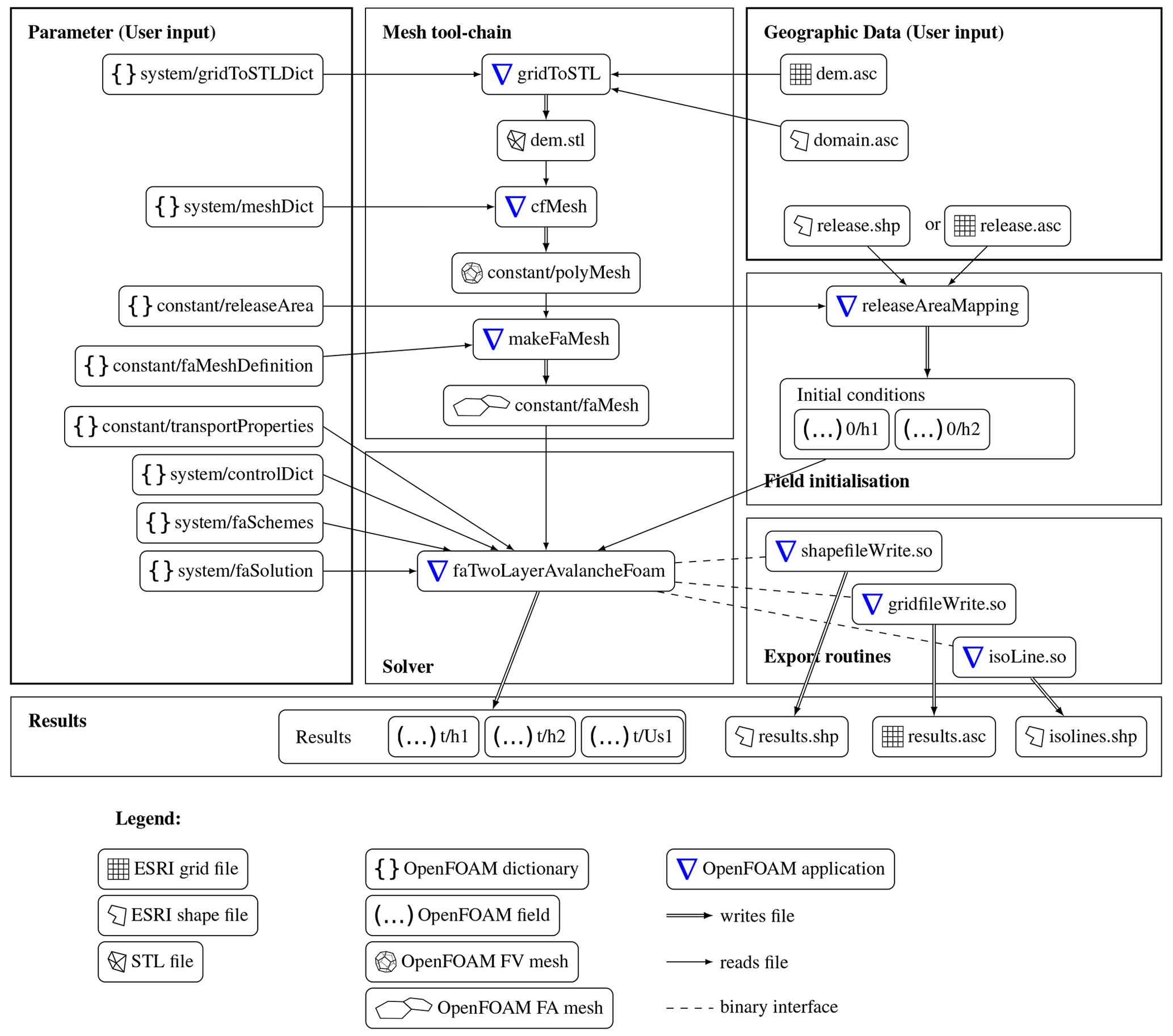
Figure 5 Pipeline of the OpenFOAM avalanche module. The pipeline has been simplified substantially since the work of Rauter et al. (2018). Most notably, all components are fully implemented in C++ and included into the module. The pipeline includes the complete workflow, starting from GIS data and returning all results to GIS data. The user can modify parameters in the respective dictionaries and geometry of the simulation domain and the initial conditions in the geographic input data. The solver can be any of the three models.

6.1 Mesh generation from terrain data

The mesh generation follows the principles of Rauter et al. (2018). In a first step a triangulation of the terrain and a boundary of the surrounding volume is generated. A new tool for this task, called gridToSTL, was written entirely in C++ and without any external dependencies. The tool requires input in the form of a polygon that defines the simulation domain and the terrain data in the form of a raster file. In contrast to the previous version, the polygon can be any kind of closed and non-intersecting polygon with an arbitrary number of edges, either convex or concave. This enables flexibility in the choice of the simulation domain, which turned out to be especially useful to cover long and windy submarine canyons.

The finite volume mesh is generated from the triangulated surface with an arbitrary mesh generator. This toolchain can be applied to the depth-integrated models presented here and was also used for the full three-dimensional model presented by Rauter et al. (2022). In this study we used the mesh generator pMesh, while Rauter et al. (2022) used cartesianMesh, both from the cfMesh toolbox (Juretić, 2015). The finite area mesh is then generated on a dedicated surface of the finite volume mesh using the tool makeFaMesh, part of the OpenFOAM finite area module.

6.2 Mapping initial conditions

Initial conditions can be set with the tool releaseAreaMapping. In addition to the functionality of previous versions, this tool is now able to read shape files and grid files and map them directly onto finite area fields to be used by any solver. All input for the tool is read from a dictionary, where further references to shape and grid files can be listed. This tool enables efficient adaption to new scenarios.

6.3 Simulation run

Once the mesh and the initial conditions are defined, the solver of choice can be run. Currently there are three solvers available in the avalanche module, the dense-flow solver faSavageHutterFoam, the suspension flow solver faParkerFukushimaFoam, and the mixed-flow solver faTwoLayerAvalancheFoam (Fig. 5 shows faTwoLayerAvalancheFoam only, but it can be replaced with any of the other two models). Physical parameters are read from the file transportProperties, general simulation settings from controlDict, and numerical algorithms and parameters from the files faSolution and faSchemes. To run the solver in parallel, the tool decomposePar has to be run before the solver, and the tool reconstructPar has to be run after the solver. In the common OpenFOAM manner, all steps for a simulation are listed in a script file named Allrun, which can be launched by the user to automatically execute the pipeline outlined here. Another script, named Allclean, can be run to clean up the simulation directory.

6.4 Postprocessing and data export

The OpenFOAM architecture allows the execution of customized code, called function objects, in every simulation step. Various function objects are made available in the avalanche module. Most importantly, this includes function objects to export simulation results as either shape or raster files. The export as shape files can be done cellwise (one polygon for each computational cell), or the numerical data can be recombined to generate isolines that are written into the shape file. Function objects can be loaded by placing the respective entry into the control dictionary. As of version v2312, all solvers are able to run in a post-processing mode, in which old results are read from a hard disc and the function objects are executed. This allows the execution of function objects in a post-processing workflow without rerunning the whole simulation.

7 Results and discussion

7.1 Dense-flow model

The dense-flow model has been applied to various cases in multiple studies. The interested reader is referred to Rauter and Tuković (2018) for lab scale simulations, Rauter et al. (2018) and Huber et al. (2018) for large-scale snow avalanche simulations, Rauter and Köhler (2020) for simulations with the deposition model, and to Shimizu (2022) for an application to pyroclastic flows.

7.2 Suspension flow model

Parker et al. (1986) simulate steady suspension flows on constantly inclined one-dimensional slopes with the model presented in Sect. 4. Four cases with uniform model parameters but different boundary conditions give a good overview of the behaviour of the model and a verification (as defined by Roache, 1997, as solving the equations right) of the presented implementation. The four simulations are conducted on one-dimensional slopes with a gradient of 5 %. The gravitational acceleration follows as $\mathit{g}=(\mathrm{0.49},\mathrm{0},-\mathrm{9.81}{)}^T$ m s⁻² (chosen to match the setup by Parker et al., 1986). The parameters suggest that the suspensions are composed of sediment in water on a scale of a small turbidity current.

Table 1 Parameters for the small-scale simulations of Parker et al. (1986).

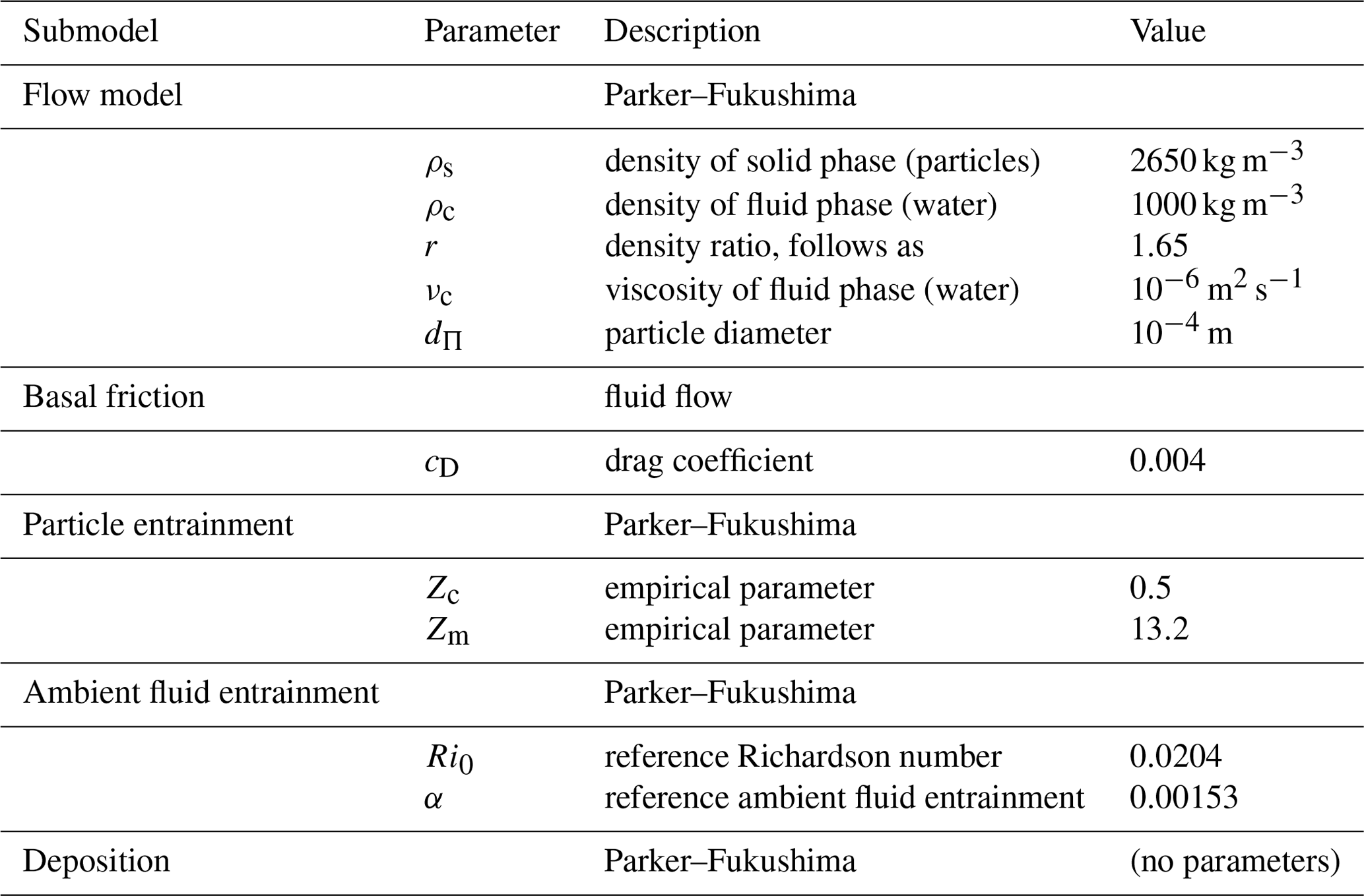
Material parameters for this setup are given in Table 1. The left boundary condition (at x=0) prescribes the inflow in terms of the height h_Π, velocity ${\stackrel{\mathrm{‾}}{\mathit{u}}}_{\mathrm{\Pi }}$, and grain flux ${\stackrel{\mathrm{‾}}{\mathit{\psi }}}_{\mathrm{\Pi }}=h_{\mathrm{\Pi }}{\stackrel{\mathrm{‾}}{\mathit{\varphi }}}_{\mathrm{\Pi }}{\stackrel{\mathrm{‾}}{\mathit{u}}}_{\mathrm{\Pi }}$, in particular as shown in Table 2. All parameters are given normalized to reference values H=2 m, U=0.874 m s⁻¹, and Ψ=0.00828 m² s⁻¹.

Table 2 Inlet boundary conditions for the small-scale simulations of Parker et al. (1986), simulating four scenarios of igniting or fading turbidity currents.

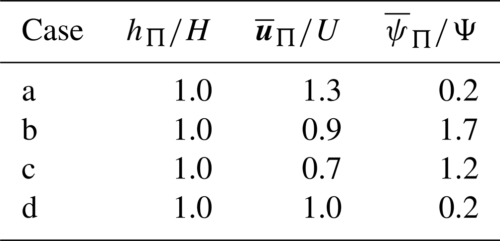
The right boundary condition is modelled as a zero gradient for all fields, mimicking an outlet boundary condition. For a basic verification of the novel implementation of the suspension model, the respective simulations are repeated and compared to the original results. We will evaluate the buoyancy assumption of Parker et al. (1986), as well as the formulation with the correct density given in here. The simulations are conducted in an unsteady manner until the flow reaches a steady state, comparable to the results reported by Parker et al. (1986). Figure 6 shows results for the four cases.

The first case, starting with a high velocity but low particle fraction increases its particle fraction quickly, as the high velocity is sufficient to erode and pick up sediment. The second case starts with a very high phase fraction, leading to a sudden ignition of the flow at $x/H=\mathrm{60}$. The height of the suspension stays low and even decreases, showing that a high phase fraction can keep the suspension concentrated at the bottom. The third and fourth case start with a low velocity and low particle phase fraction, respectively, and the suspension fades out quickly. The height of the flow increases in both cases where the flow fades out, indicating that the momentum of the flow is diffused over larger volumes of fluid. This is consistent with the expected scaling of fluid entrainment with the Richardson number.

It can be seen that results of Parker et al. (1986) are reproduced with only small deviations. The OpenFOAM solver yields sharper edges than the implementation of Parker et al. (1986), especially visible in Fig. 6b. This small difference is most likely attributable to the numerical solution method or the numerical resolution. The correction of the time derivative and advection term with $(\mathrm{1}+r{\stackrel{\mathrm{‾}}{\mathit{\varphi }}}_{\mathrm{\Pi }})$ has only a minimal influence on the model results. This is reasonable, considering the low value for the buoyant density ratio r=1.65 in these cases. These simulations suggest that the model of Parker et al. (1986) is implemented correctly. However, this can not be seen as a validation (Roache, 1997) of the model.

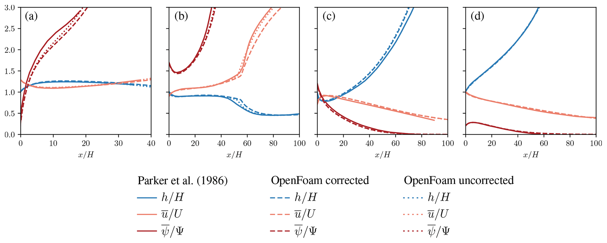
Figure 6 Numerical simulation of the four test cases presented by Parker et al. (1986) with OpenFOAM, with and without the buoyancy assumption (corrected and uncorrected, respectively). The results of Parker et al. (1986) are reproduced with good accuracy. The buoyancy assumption fits well to the conditions of these numerical experiments.

7.3 Two-layer model

7.3.1 Synthetic tests and sensitivity study

In order to better understand the two-layer model, we will conduct tests on synthetic topographies. The topography is based on a parabola with a length of L=4000 m and a height of H=2000 m, with an additional flat runout area of 2000 m. The slope has a width of 2000 m, leading to a simulated region of $x=[-\mathrm{4000},\mathrm{2000}]$ m and $y=[-\mathrm{1000},\mathrm{1000}]$ m. In addition, the influence of topographic structures will be investigated, as terrain features often initialize the formation of suspension flows (e.g. powder snow avalanches). A bump in the surface is created by superposing the parabola with a Secans hyperbolicus $\mathrm{sech}\left(x\right)=\mathrm{2}/\left(\exp \left(x\right)+\exp (-x)\right)$ at $X_{\mathrm{p}}=-\mathrm{2700}$ m with a height of H_p=150 m and a length of L_p=200 m:

$$\begin{array}{}\text{(49)}& {\displaystyle }z=H_{\mathrm{p}}\mathrm{sech}\left({\displaystyle \frac{x-X_{\mathrm{p}}}{L_{\mathrm{p}}}}\right)+\left\{\begin{array}{ll}H{\left({\displaystyle \frac{x}{L}}\right)}^{\mathrm{2}}& \text{for }x<\mathrm{0},\\ \mathrm{0}& \text{otherwise,}\end{array}\right.\end{array}$$

inspired by the experiments of Viroulet et al. (2017). All boundaries are implemented as von Neumann (zero gradient) boundary conditions.

The release area (initial condition) of the slide was formed by a rectangle between $x=[-\mathrm{3900},-\mathrm{3500}]$ m and $y=[-\mathrm{500},\mathrm{500}]$ m and an initial dense-flow height of h_Φ=5 m within that square. All other flow fields are set to zero. The parameters, roughly corresponding to snow avalanches, are given in Table 3, if not mentioned otherwise. The value for the coupling factor s_f is varied, and the sensitivity of the model to this parameter is investigated. Entrainment and deposition to and from the static layer are not included in this section for simplicity. The simulations were run for 90 s.

Besides the flow thickness, velocity, and phase fraction, we can analyse the dynamic pressure, which is an important indicator of the destructive potential of the flow. It is defined as

$$\begin{array}{}\text{(50)}& {\displaystyle }{p}_{\mathrm{d}\mathrm{\Phi }}={\mathit{\rho }}_{\mathrm{\Phi }}|{\stackrel{\mathrm{‾}}{\mathit{u}}}_{\mathrm{\Phi }}{|}^{\mathrm{2}}\end{array}$$

for the dense flow and as

$$\begin{array}{}\text{(51)}& {\displaystyle }{p}_{\mathrm{d}\mathrm{\Pi }}=\left({\mathit{\rho }}_{\mathrm{g}}{\mathit{\varphi }}_{\mathrm{\Pi }}+{\mathit{\rho }}_{\mathrm{c}}\left(\mathrm{1}-{\mathit{\varphi }}_{\mathrm{\Pi }}\right)\right)|{\stackrel{\mathrm{‾}}{\mathit{u}}}_{\mathrm{\Pi }}{|}^{\mathrm{2}}\end{array}$$

for the powder cloud (e.g. Jóhannesson et al., 2009). In particular we evaluate the dynamic peak pressure, which is defined as the maximum of the dynamic pressure at a fixed point over time. Important limits that are used in the definition of hazard zones (e.g. in Austria) are 1 kPa (yellow zone) and 10 kPa (red zone) (Jóhannesson et al., 2009). Notably, the shape factor should be applied to the dynamic pressure for consistency, increasing all simulated pressures by 25 %. However, this is neglected in order to be consistent with previous work and the definition of hazard zones.

Results for a simple parabola (without surface bump) are shown in Fig. 7 for three values of s_f (10⁻⁵, 10⁻⁴, 10⁻³). This set of simulations allows some valuable conclusions on the model and in particular the coupling model. All simulations start with a dense flow that eventually feeds the powder cloud. The feeding rate of the powder cloud varies strongly due to the variation of the parameter s_f.

For a low value of s_f, the dense flow is not able to generate a strong powder cloud with a considerable particle phase fraction and thus density. A suspension flow develops eventually; however, it consists almost entirely of air, without any ice particles. Basically, this can be seen as a layer of air that is dragged along by the dense flow. The velocity, dynamic pressure, and runout distance of this layer are correspondingly low. As shown before, the flow height of the suspension layer grows strongly for fading flows, indicating a strong diffusion of momentum.

Increasing the value for s_f up to 10⁻⁴ leads to higher phase fractions up to 0.004, roughly corresponding to a density of 4 kg m⁻³. Further increasing the value to 10⁻³ leads to phase fractions of up to 0.02 and densities of 20 kg m⁻³, however only for short periods. Notably, these are depth-averaged phase fractions and densities, and the respective values close to the surface might be considerably higher. The corresponding dynamic pressure of the powder cloud is still low, and only the simulation with the highest coupling factor s_f is able to generate a red zone that extends beyond the red zone of the dense flow. These results seem reasonable, considering the average slope gradient of 50 % and the absence of any topographic features that might enhance the feed of the powder cloud. More powerful powder snow avalanches can be expected on steeper slopes and on slopes with high topography variations (e.g. steep cliffs or rough terrain). Further simulations (not shown here) revealed that the powder cloud increases substantially with higher slope gradients.

Results for the slope with a bump are shown in Fig. 8. The model shows a high sensitivity to the terrain, and this case represents natural slopes with varying gradients better. All simulations create a considerable powder cloud with high phase fractions. The highest phase fraction is reached shortly after the top of the bump where the negative centrifugal forces are strongest and the basal pressure the lowest. The phase fraction reaches up to 0.05, roughly corresponding to a density of 50 kg m⁻³. A shock is formed at the bump in the suspension layer due to the high gradient in the phase fraction, leading to a considerable pressure gradient that decelerates the flow. In all simulations the dynamic powder cloud pressure exceeds 10 kPa, and the respective high pressure zone extends beyond the dense-flow runout. The 1 kPa zone of the powder cloud reaches considerable runouts beyond the dense flow.

Table 3 Parameters for the two-layer model for synthetic cases on parabolas and for the Wolfsgruben and Eiskar avalanches.

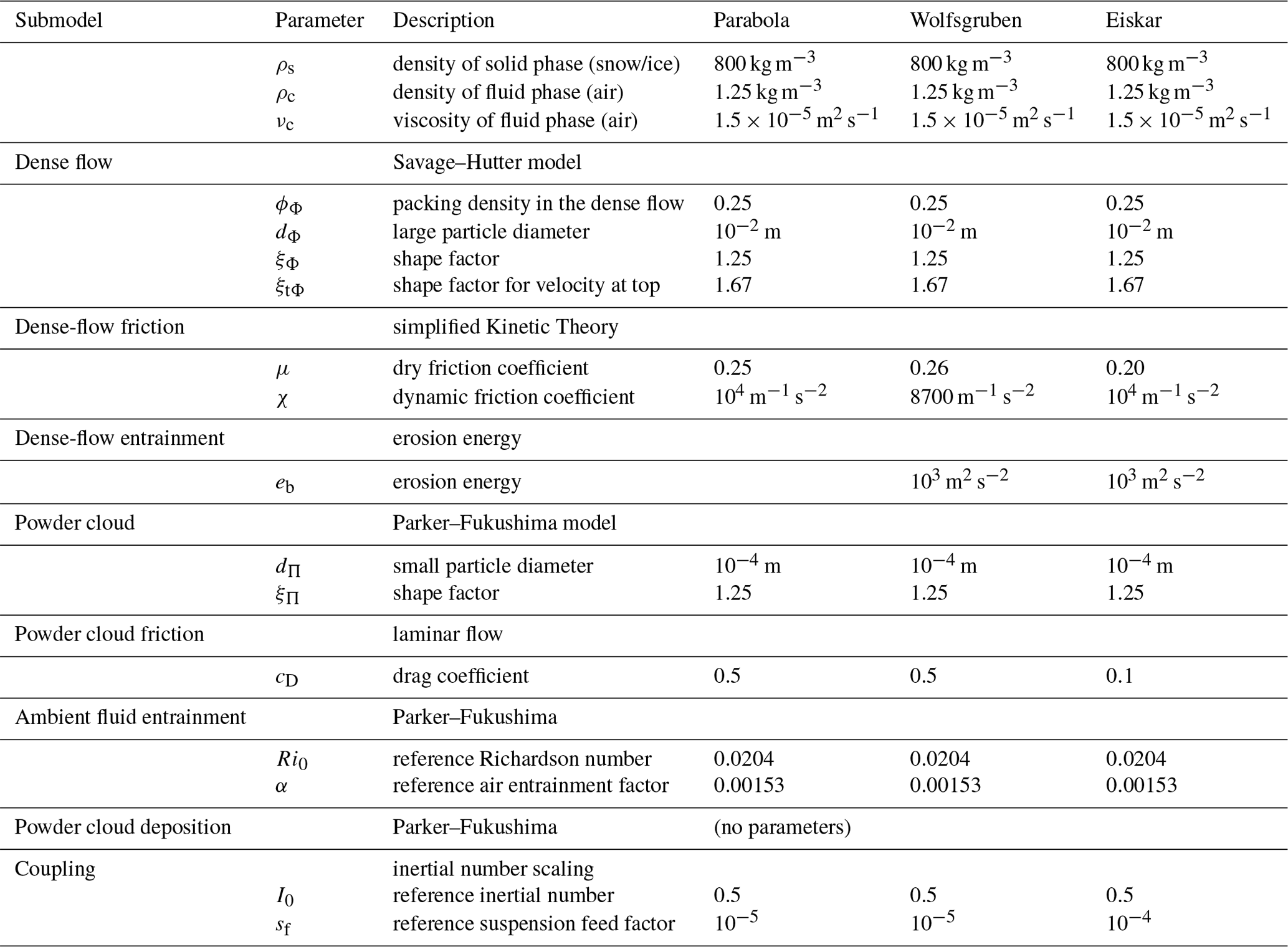
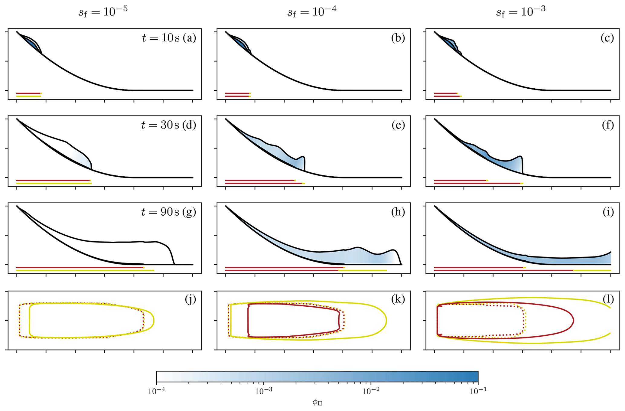
Figure 7 Numerical simulations of mixed-snow avalanches on a parabolic slope with the two-layer model. The parameter s_f was varied between 10⁻⁵ (a, d, g, j), 10⁻⁴ (b, e, h, k), and 10⁻³ (c, f, i, l). Panels (a)–(i) show the cross section in the middle of the slide. The slope is shown as the lower black line. The flow thickness h_Φ is shown as an offset of the surface magnified by a factor of 20; the flow thickness h_Π is shown above the dense flow magnified by a factor of 10. The powder cloud is coloured according to the phase fraction ϕ_Π. The red and yellow lines below the slope mark the regions of high dynamic peak pressure p_d>10 kPa and intermediate dynamic pressure p_d>1 kPa for the dense flow (top) and the powder cloud (bottom) respectively. Panels (j)–(l) show the regions of high and intermediate dynamic peak pressure (dashed: dense flow, continuous: powder cloud) from the top. One tick on the axis equals 1000 m.

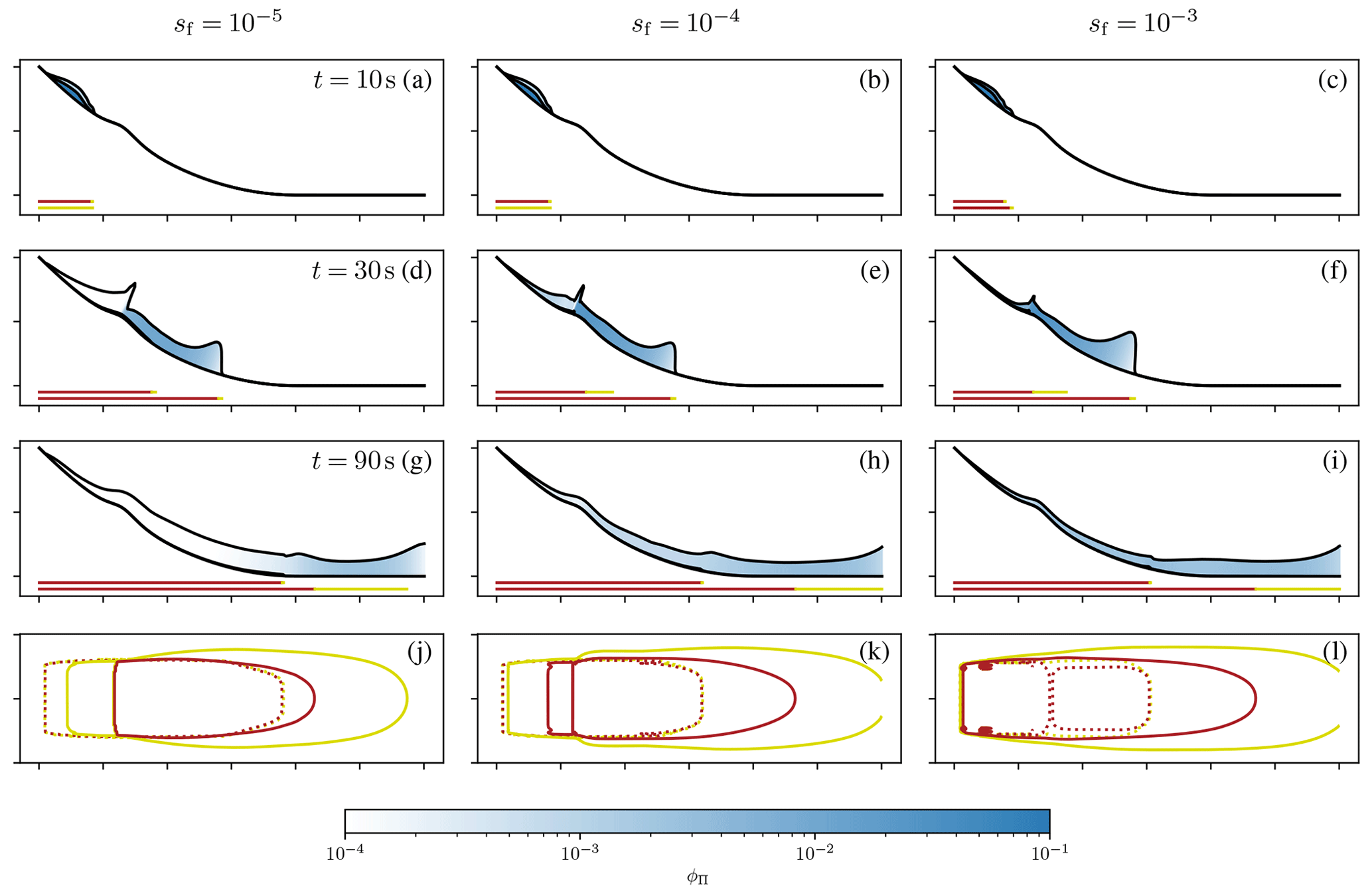
Figure 8 Numerical simulations of snow avalanches on a parabolic slope with a bump with the two-layer model. Same as Fig. 7 but with a bump with height 150 m and length 200 m at $x=-\mathrm{2700}$ m.

The results on synthetic terrain show a reasonable behaviour of the model, both in terms of parameterization and response to the terrain. The effect of the terrain is well visible and corresponds to the assumptions from which the model was derived. The sensitivity of the model to the parameter s_f is well pronounced, and this factor can be utilized to fit the model to real-world observations. A value between 10⁻⁴ and 10⁻⁵ seems reasonable for the parameter of the coupling model.

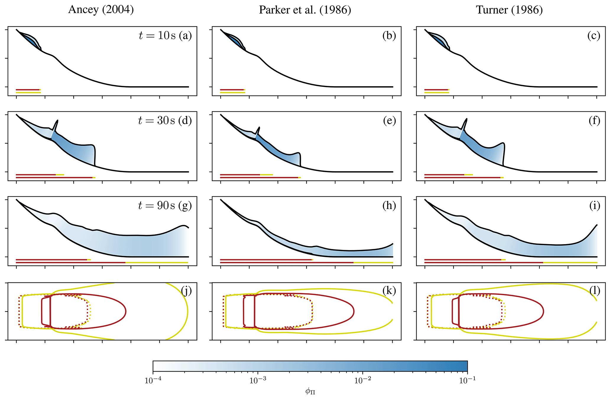
Finally, we use the synthetic cases to showcase the sensitivity of the model to the air entrainment. Figure 9 shows the simulation on the synthetic terrain with the three presented air entrainment models. The differences are small but noticeable. In particular, the entrainment is stronger with the model of Ancey (2004), however, which is just a question of parameterization. More importantly, the model of Turner (1986) shows a more pronounced flow head. The Richardson number is low in the head, and the relation of Turner (1986) predicts the strongest entrainment at low Richardson numbers (see Fig. 4). Generally, all relations appear reasonable and well in line with each other. We will continue with the entrainment model of Parker et al. (1986) from here on. Considering an optimization of air entrainment parameters to real events, it might be useful to apply the model of Ancey (2004) instead, as it provides the clearest parameterization.

Figure 9 Numerical simulations of snow avalanches on a parabolic slope with a bump. Same as Fig. 8 but with a variation of the air entrainment model and a fixed parameter s_f.

7.3.2 Real-case example: the 1988 Wolfsgruben avalanche

The 1988 Wolfsgruben avalanche represents an important event in Austria, as it was the trigger for many developments and used repeatedly as a benchmark. The event, or at least its dense core, was featured by Fischer et al. (2015) and Rauter et al. (2018). Here we revisit the event with the new two-layer model and include the powder cloud into the analysis. The avalanche is characterized by a channellized, steep slope with an angle of 30° that transitions fairly abruptly to the flat valley floor and the opposite slope.

The preprocessing and simulation setup follows Rauter et al. (2018) but with the novel tool chain and an extended simulation domain to cover the full runout of the powder cloud. The initial release areas of the avalanche and the erodible snow covers are the same, following the linear approach:

$$\begin{array}{}\text{(52)}& {\displaystyle }\begin{array}{rl}{h}_{\mathrm{\Sigma }}(x,y,z,t=\mathrm{0})& =\left(h_{\mathrm{\Sigma }}\left(z_{\mathrm{0}}\right)+{\displaystyle \frac{\partial h_{\mathrm{\Sigma }}}{\partial z}}\left(z-z_{\mathrm{0}}\right)\right)\\ & \cos \left(\mathit{\theta }\left(x,y,z\right)\right),\end{array}\end{array}$$

where z is the surface elevation and z₀ the elevation of a reference point with the base value h_Σ(z₀). The growth rate $\frac{\partial h_{\mathrm{\Sigma }}}{\partial z}$ defines the change with elevation from that point. θ is the angle between the gravitational acceleration and the surface-normal vector. For the 1988 Wolfsgruben avalanche, we use the snow cover parameters h_Σ(z₀)=1.61 m, z₀=1289 m, and $\frac{\partial h_{\mathrm{\Sigma }}}{\partial z}=\mathrm{8}\times {\mathrm{10}}^{-\mathrm{4}}$.

The model parameters are shown in Table 3. The dense-flow parameters have been optimized in a previous study (Fischer et al., 2015; Rauter et al., 2018), however for a model ignoring the powder cloud. The addition of the powder cloud could lead to different optimal dense-flow parameters. However, that is out of the scope of this work, and we assume that the previously used parameters fit sufficiently well. The suspension parameters are deduced from literature where possible (density, grain diameter). The coupling parameter $s_{\mathrm{f}}={\mathrm{10}}^{-\mathrm{5}}$ was found after running some simulations, starting from the values derived from the simulations on synthetic cases. A higher value leads to an unrealistically short dense-flow runout and a lower value to a severe underestimation of the suspension impact pressure. The friction coefficient c_D was chosen to be sufficiently large for the powder cloud to not completely decouple from the dense core. Apart from this effect, the simulation is rather insensitive to the friction coefficient c_D.

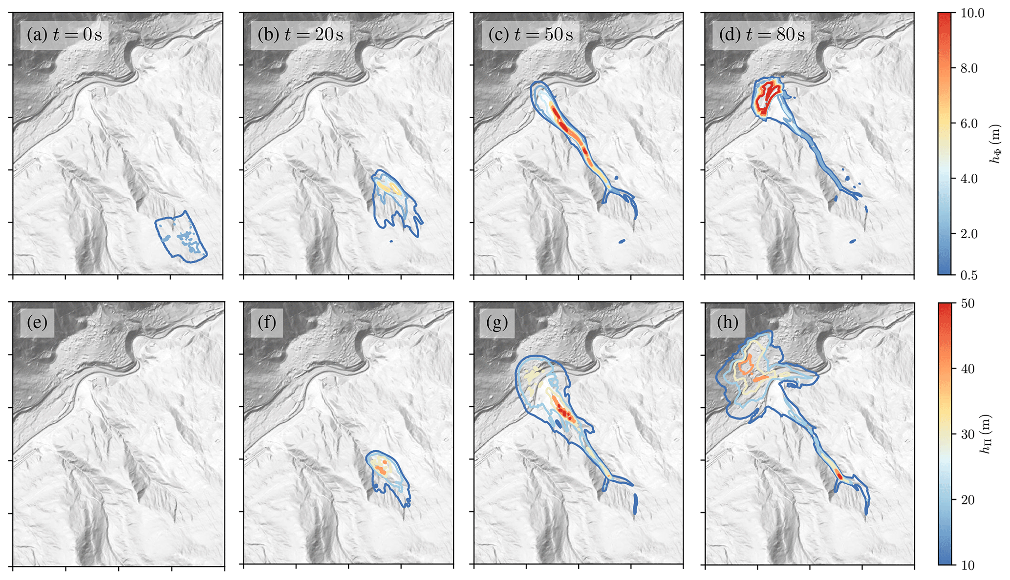
Figure 10 Numerical simulation of the Wolfsgruben avalanche with the two-layer model. The first row (a–d) shows the height of the dense-flow layer; the second row (e–h) shows the height of the powder cloud layer. Each tick on the x and y axes corresponds to 500 m. Terrain data: Amt der Tiroler Landesregierung (AdTLR).

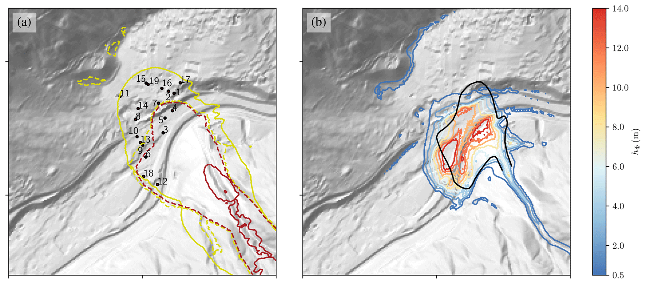
Figure 11 (a) The dynamic peak pressure of the suspension layer (solid lines) and the dense-flow layer (dashed line). The yellow line marks the 1 kPa isoline and the red line the 10 kPa isoline. (b) The deposition of the avalanche (at t=180 s). Terrain data: AdTLR.

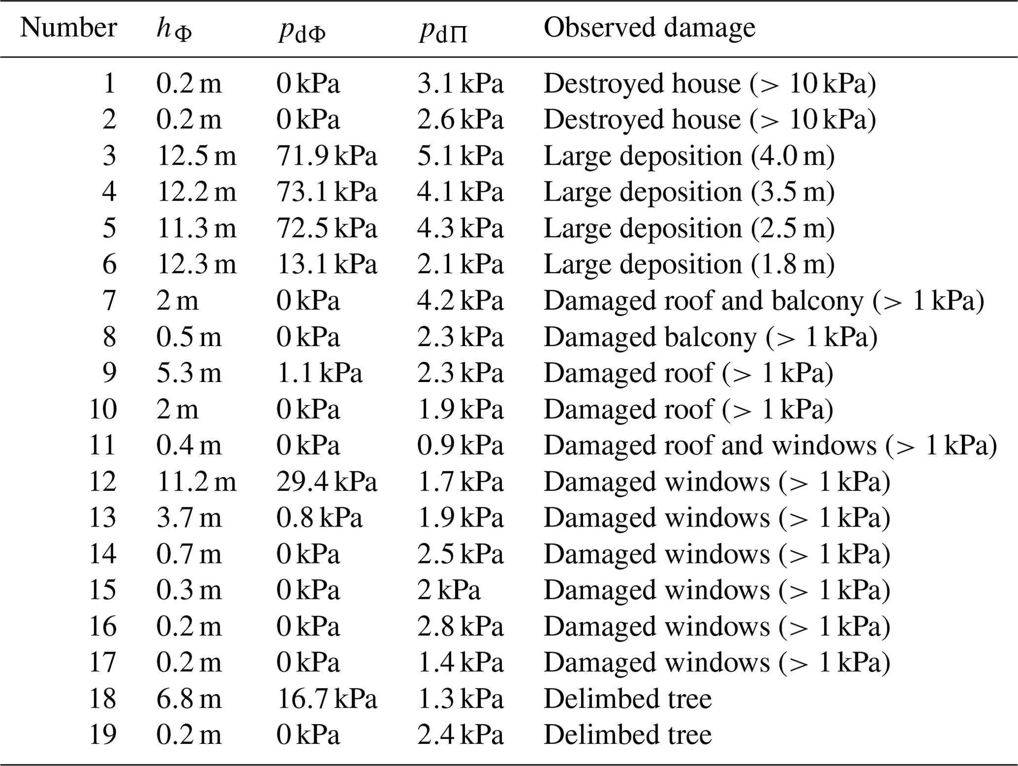
Table 4 Simulated dynamic peak pressure at the location where damage was observed.

Four time steps of the simulation are shown in Fig. 10, displaying isolines of the dense-flow height h_Φ (a–d) and the suspension flow height h_Π (e–h). The avalanche starts as a dense flow and rapidly accelerates due to the steep release area (Fig. 10a). Shortly after the release a strong suspension layer is formed that further accelerates beyond the velocity of the dense-flow layer (Fig. 10b, f). After roughly 40–50 s the avalanche reaches the bottom of the valley (Fig. 10c, g). The powder cloud outruns the dense flow and hits the valley floor first. The dense flow is stopped quickly due to the high granular friction, while the powder cloud keeps running up on the opposite slope for approximately 50 m of elevation. Both flows experience a shock that increases the flow height in the valley floor drastically. The deposition (i.e. the dense-flow height in the last time step) reaches up to 15 m, however, which does not account for the difference between flow (≈200 kg m⁻³) and deposition density (≈600 kg m⁻³).

Results for the dense flow can be validated by a comparison with the deposition (see Fig. 11b), and they are similar to previous studies with the same model and the model SamosAT (Fischer et al., 2015; Rauter et al., 2018). Results for the powder cloud are more difficult to validate. Traces of the powder cloud that can be identified in the field are limited and not straightforward to interpret, as no clear deposition pattern emerges from suspended flows. Further, the respective deposition can hardly be related to the impact pressure and thus the destructive potential of the flow. Therefore, we compare the simulated dynamic pressure with observed building damages from the respective avalanche (see Fig. 11a). This includes not only the suspension layer but also the dense flow. An evaluation of the dynamic peak pressure and the deposition height at damaged objects is shown in Table 4.

The dense flow does not reach the two destroyed buildings (Point 1 and 2 in Fig. 11a and Table 4) and stops about 20 m short. Points 12 and 18 were only slightly damaged by the suspension flow in reality but severely hit by the dense flow in the simulation, showing that the simulation tends too strongly to the left side (viewed in the flow direction). The deposition height that was recorded at selected points (Table 4) is matched well, assuming a compaction of the avalanche by a factor of 3 after deposition.

The suspension layer shows a very limited zone of high dynamic pressure (>10 kPa) but an extended zone of intermediate dynamic pressure (1–10 kPa). The model predicts dynamic pressures of 1–4 kPa where balconies and roofs have been damaged and 1–3 kPa where windows have been destroyed. This corresponds well with engineering estimations of resistance capabilities of the respective parts: windows are assumed to break at 2–4 kPa and doors, walls, and roofs at 3–6 kPa (Sovilla et al., 2015). The dynamic pressure of the suspension layer at the destroyed buildings (Point 1 and 2 in Fig. 11) is not sufficient to destroy the respective brick structures (25–45 kPa). These high values strongly indicate that the dense flow or a saltation layer must be responsible for these high impact pressures (see pictures in Fischer et al., 2015). Therefore, we conclude that the simulated suspension layer reaches all observed traces of the powder cloud without covering the region where no traces could be observed.

7.3.3 Real-case example: the 2019 Eiskar avalanche

On 15 January 2019, the Eiskar avalanche occurred after intense snowfall and a rapid temperature drop (Oesterle, 2019). The Eiskar avalanche differs substantially from the Wolfsgruben avalanche regarding topography and thus provides a good supplement to that case. The avalanche was initiated by a slab on the right-hand side of the avalanche path (looking in the flow direction) that fell onto a larger snow field. From there, the avalanche slope continues with an inclination of approximately 25° for 1500 m until reaching a flatter slope of 10°. The dense-flow avalanche ran 1000 m on the flattening slope, and the powder flow exceeded the dense flow by another 500 m, reaching the village of Ramsau. The powder cloud destroyed a wooden building, damaged a hotel, and knocked over a bus. The dynamic pressure required for the damage was estimated at 1–3 kPa. Areal pictures were taken after the event, which allowed the estimation of the initial snow cover, the release area, and the deposition. The data were used to derive parameters for the snow cover function (Eq. 52), h_Σ(z₀)=1.60 m, z₀=1275 m, and $\frac{\partial h_{\mathrm{\Sigma }}}{\partial z}=\mathrm{2}\times {\mathrm{10}}^{-\mathrm{3}}$, to reach a snow cover thickness of approximately 2.7 m at an elevation of 2200 m (Oesterle, 2019). Other aspects of the simulation, such as the preparation of the terrain data, match the simulation of the Wolfsgruben avalanche.

The first simulation (not shown) was conducted with the same parameters as for the Wolfsgruben avalanche. However, these parameters lead to a severe underestimation of the powder cloud, running short by approximately 400 m. Simulations with the model SamosAT (Sampl and Zwinger, 2004) showed similar results with the standard parameters (Oesterle, 2019). Therefore, the friction coefficients and the coefficient for the suspension feed were adjusted (see Table 3) to reach an appropriate runout and dynamic pressure at the observed impacts.

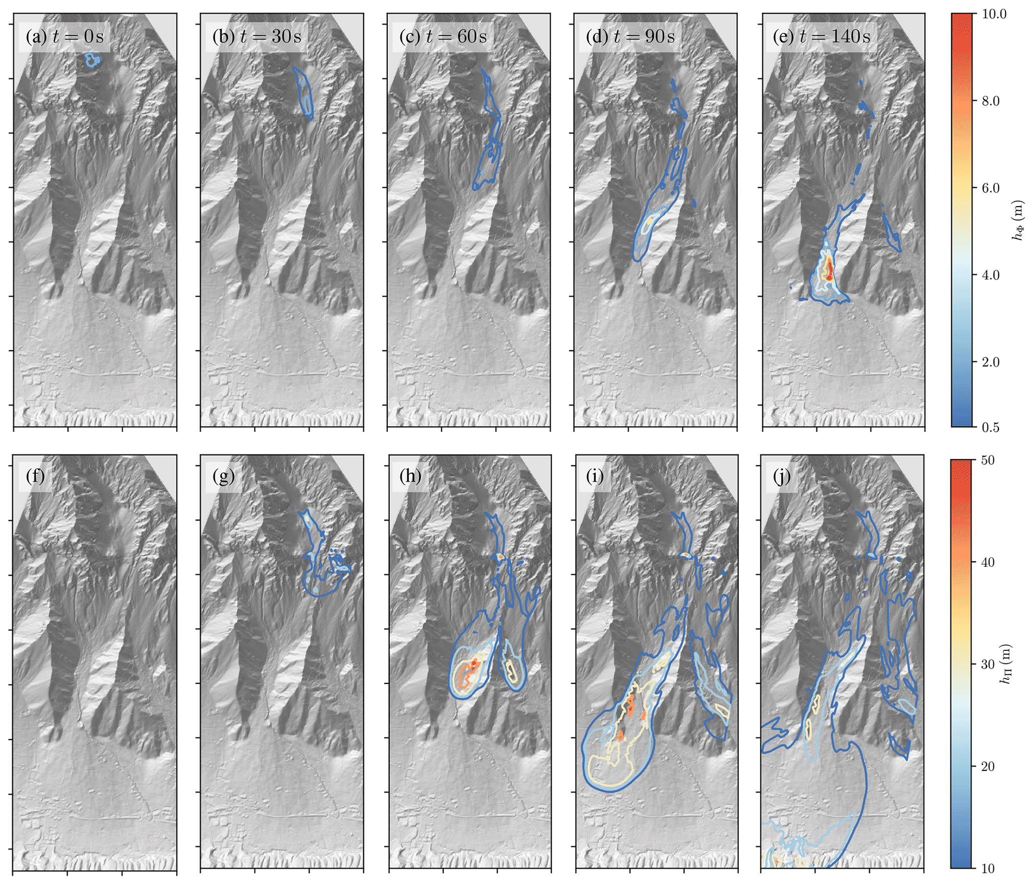
Figure 12 Numerical simulation of the Eiskar avalanche with the two-layer model. The first row (a–e) shows the height of the dense-flow layer; the second row (f–j) shows the height of the powder cloud layer. Each tick on the x and y axes corresponds to 500 m. Terrain data: Land Steiermark/GIS-Steiermark.

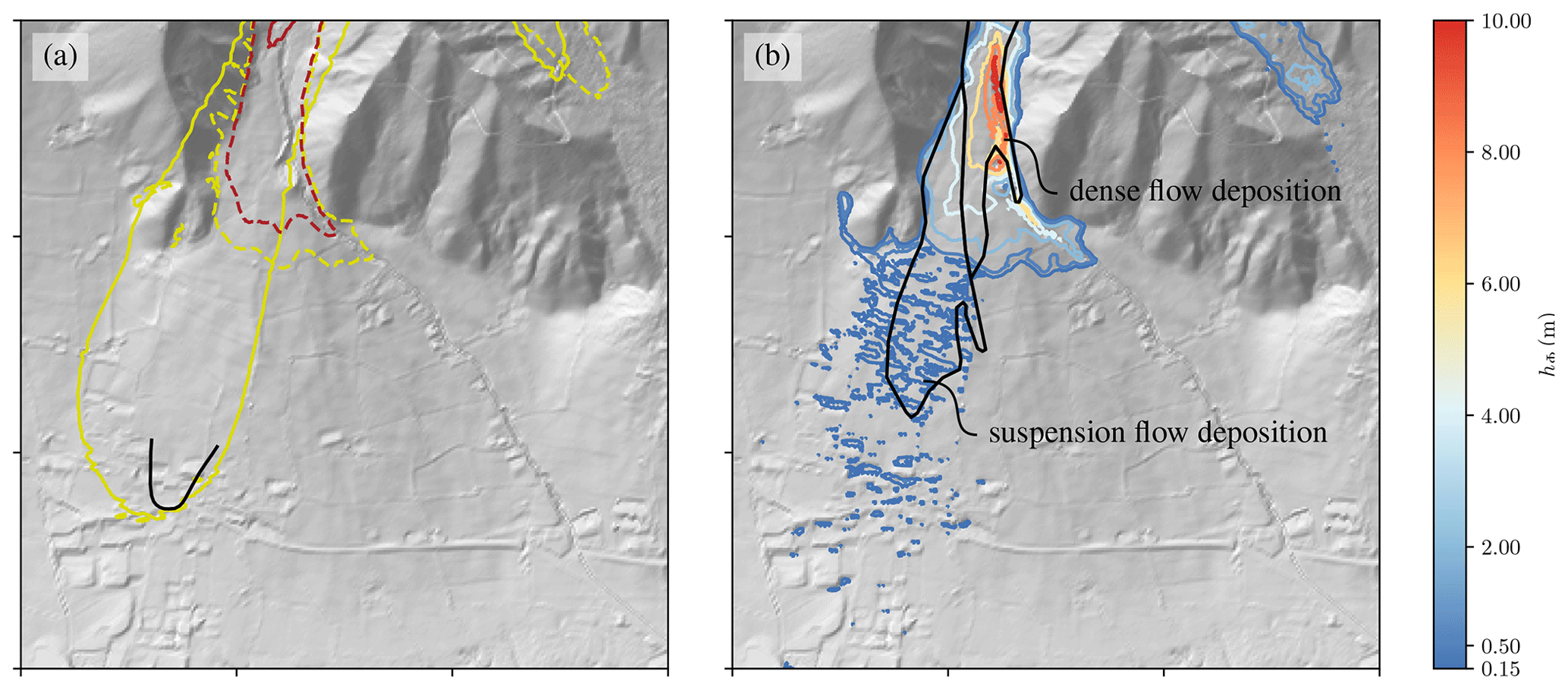
Figure 13 (a) The dynamic peak pressure of the suspension layer (solid lines) and the dense-flow layer (dashed line). The yellow line marks the 1 kPa isoline and the red line the 10 kPa isoline. The black line marks the limit of the estimated 1 kPa isoline following observations. (b) The deposition of the avalanche (at t=200 s). The black polygons mark regions of dense-flow deposition (above) and powder cloud deposition (below). Terrain data: Land Steiermark/GIS-Steiermark.

Five time steps of the simulation are shown in Fig. 12 in terms of the dense-flow height h_Φ (a–e) and the suspension flow height h_Π (f–j). The collapsing slab (Fig. 12a) falls down the steep cliff onto a larger snow field where it can entrain additional snow. After around 30 s the avalanche reaches a second cliff, and a powder cloud starts to emerge (Fig. 12b, g). The suspension layer keeps growing substantially in the slope section with an inclination of 25° (Fig. 12c, h) and starts to detach when reaching the flatter slope of the 10° inclination. The suspension layer reaches the village of Ramsau after approximately 90 s (Fig. 12i, j), while the dense flow comes to a halt at the exit of the valley (Fig. 12d, e). Interestingly the dense flow is pushed towards the left by terrain features at the exit of the valley, while the suspension layer is essentially unaffected by these small obstacles.

The corresponding zones of dynamic pressure are shown in Fig. 13a. The 1 kPa isoline of the suspension layer extends far into the village. This fit was used as a benchmark to determine the optimal model parameters and thus matches observations well. The final deposition of the model is shown in Fig. 13b and compared to the observed deposition. The observations distinguish between suspension and dense-flow depositions (Oesterle, 2019), and the same can be done in the numerical model. The dense-flow layer leaves behind up to 10 m thick deposits (to be corrected by a factor of $\mathrm{1}/\mathrm{3}$ to match the deposition density) with sharp edges, while the suspension generates deposits with 0.1–0.2 m thickness (to be corrected as well) that fade out gradually. Both the position of the respective deposits and their shape match the observations.

Overall, the model is able to reproduce the observed flow traces, from the dynamic pressure to the varying snow deposits, in a single simulation. However, the model parameters had to be fitted to achieve these results. The friction parameters have to be substantially lower than in the Wolfsgruben case, and the coupling factor has to be an order of magnitude higher. This indicated that conditions were substantially different between the two cases or that the model does not cover some important processes.

8 Conclusions

This work provides an overview of the implementation of the granular dense-flow model of Savage and Hutter (1989, 1991) and the suspension flow model of Parker et al. (1986) into OpenFOAM. Further, the models have been combined by means of a novel coupling mechanism to provide a simple yet effective mixed-snow avalanche model. These three models form the core of the OpenFOAM avalanche module. The module is accompanied by a new toolchain that substantially simplifies the practical application of the framework. The integration of geographic information system (GIS) file types into the OpenFOAM framework enables a simple and deep integration in existing workflows. Moreover, the dependencies on third-party libraries for GIS support were removed as they were often missing on computational clusters. In comparison to the work of Rauter et al. (2018), the models and all tools are integrated into OpenFOAM to simplify installation. The physical models are highly modular. Tweaking and replacing specific empirical relation or process models are a core feature of the framework and highly encouraged.

The implementation of the suspension flow model of Parker et al. (1986) was verified by repeating published results, assuring the absence of implementation errors. A novel two-layer model was developed and evaluated with simple synthetic cases. The results are reasonable and follow the expectations set in the model. Further investigations have been conducted with two different real-case avalanches. The reach of the dense-flow layer and the suspension layer matched the observed runout in both cases with good accuracy, although a quantitative comparison was not conducted. The dense flow of the Wolfsgruben avalanche came short of approximately 20 m. The impact pressure of the suspension flow is reasonable considering the observed damage. Results for the Eiskar avalanche similarly match observations well if the parameters are fitted accordingly.

The good results are strongly linked to the parameterization, which is highly uncertain due to the limited experience with mixed-snow avalanche models in general and this model in particular. A wide variety of results can be achieved by tweaking the parameters of the model, and substantial investigations will be required to find the appropriate parameters for the large number of semi-empirical relations embedded in the flow models. Substantially different parameters were required to yield reasonable results in both cases, a well-known problem in gravitational mass flow modelling (Scheidegger, 1973; Lucas et al., 2014). Further, snow properties and temperatures might have been substantially different between the two avalanche events. In this regard we see a strong opportunity to substantially improve the two-layer model. Temperature has a strong influence on the particle diameter distribution in snow avalanches and will thus have a high effect on the mobility and the ability to generate suspension flows (Steinkogler et al., 2015a, b).

The dense-flow runout and especially its dynamic pressure at a specific point are very sensitive to the parameters. This is related to the strong friction that rises rapidly in flat regions, where the driving gravitational acceleration also vanishes. The suspension cloud is less sensitive to such influences, as the friction is lower and independent of the inclination and the basal pressure. Therefore, the suspension runout is less sensitive to the parameters.

For practical applications we advise to use the existing guidelines for the dense-flow parameters (e.g. Salm et al., 1990). For snow avalanches with a high potential to generate powder snow clouds, we suggest to apply the suspension and coupling parameters as used in the Eiskar case. It should be noted that the suspension model absorbs mass from the dense-flow model, which reduces the respective runout. Therefore, it might be reasonable to simulate scenarios with less powder flow generation to not underestimate the runout of the dense core. Finally, it should be kept in mind that the results of the model are accompanied by a high number of uncertainties and that they should be used accordingly. Nevertheless, the simulations presented here recreate the processes of the events well and provide a considerable amount of additional information.

Generally, the model and the whole framework aim to be very flexible to provide researchers with a strong platform to develop and evaluate novel friction, entrainment, and coupling models. The introduced coupling model represents a reasonable approach that yields promising results, but there might be big opportunities for improvement. We hope that the framework can provide a starting point for other researchers to develop new coupling mechanisms with better performance. Further, new solvers can be implemented on the basis of the framework, e.g. multiphase models for debris flows (e.g. Pudasaini, 2012; Kowalski and McElwaine, 2013; Iverson and George, 2014) as done by Garcés et al. (2023) with faDebrisFoam or landslide tsunamis (e.g. George et al., 2017). The toolchain and post-processing routines presented here can be reused with these models, and additional pre- and postprocessing utilities can be added to enlarge the functionality of the whole framework.

Appendix A: Simplified computation of centrifugal forces

The basal pressure is computed following Eq. (14) in the model of Rauter and Tuković (2018). For the Parker et al. (1986) model we tried to achieve a simpler model that can also be combined with the empirical process models in the powder cloud but still follows the general approach. Neglecting the small longitudinal pressure gradient term and removing the indices marking the layer, Eq. (14) can be simplified to

$$\begin{array}{}\text{(A1)}& {\displaystyle }{\displaystyle }h\mathit{\rho }{\mathit{g}}_{\mathrm{n}}-\mathit{\xi }\mathit{\rho }{\mathbf{\nabla }}_{\mathrm{n}}^{\mathrm{\Gamma }}\cdot \left(h\stackrel{\mathrm{‾}}{\mathit{u}}\stackrel{\mathrm{‾}}{\mathit{u}}\right)=-{\mathit{n}}^{\mathrm{\Gamma }}{p}_{\mathrm{\Phi }}.\end{array}$$

We want to compare this equation to the following equation with an effective gravitational acceleration that contains the effects of centrifugal forces:

$$\begin{array}{}\text{(A2)}& {\displaystyle }h\mathit{\rho }{\mathit{g}}_{\mathrm{eff}}=-{\mathit{n}}^{\mathrm{\Gamma }}{p}_{\mathrm{\Phi }}.\end{array}$$

Setting n^Γ p_Φ in Eqs. (A1) and (A2) equal to one another yields

$$\begin{array}{}\text{(A3)}& {\displaystyle }h\mathit{\rho }{\mathit{g}}_{\mathrm{eff}}=h\mathit{\rho }{\mathit{g}}_{\mathrm{n}}-\mathit{\xi }\mathit{\rho }{\mathbf{\nabla }}_{\mathrm{n}}^{\mathrm{\Gamma }}\cdot \left(h\stackrel{\mathrm{‾}}{\mathit{u}}\stackrel{\mathrm{‾}}{\mathit{u}}\right).\end{array}$$

After approximating ${\mathbf{\nabla }}_{\mathrm{n}}^{\mathrm{\Gamma }}\cdot \left(h\stackrel{\mathrm{‾}}{\mathit{u}}\stackrel{\mathrm{‾}}{\mathit{u}}\right)$ as $h{\mathbf{\nabla }}_{\mathrm{n}}^{\mathrm{\Gamma }}\cdot \left(\stackrel{\mathrm{‾}}{\mathit{u}}\stackrel{\mathrm{‾}}{\mathit{u}}\right)$ and dividing by h ρ, we can write

$$\begin{array}{}\text{(A4)}& {\displaystyle }{\mathit{g}}_{\mathrm{eff}}\approx {\mathit{g}}_{\mathrm{n}}-\mathit{\xi }{\mathbf{\nabla }}_{\mathrm{n}}^{\mathrm{\Gamma }}\cdot \left(\stackrel{\mathrm{‾}}{\mathit{u}}\stackrel{\mathrm{‾}}{\mathit{u}}\right).\end{array}$$

A further approximation neglects the shape factor ξ, finally leading to the effective gravitational acceleration as described by Eq. (26).