Analysis of model error in forecast errors of extended atmospheric Lorenz 05 systems and the ECMWF system

Forecast error growth as a function of lead time of atmospheric phenomena is caused by initial and model errors. When studying the initial error growth, it may turn out that small-scale phenomena, which contribute little to the forecast product, significantly affect the ability to predict this product. The question under investigation is whether omitting these atmospheric phenomena will improve the predictability of the resulting value. The topic is studied in the extended Lorenz (2005) system. This system shows that omitting small spatiotemporal scales that significantly affect prediction ability will reduce predictability more than modeling it. In other words, a system with model error (omitting phenomena) will not improve predictability. A hypothesis explaining and describing this behavior is developed, with the difference between systems (model error) produced at each time step seen as the error of the initial conditions. The resulting model error is then defined as the sum of the increments of the time evolution of the initial conditions so defined. The hypothesis is compared to the fit parameters that define the model error in certain approximations of the average forecast error growth. Parameters are interpreted in this context, and the approximations are used to estimate the errors described in the hypothesis. A method is proposed to distinguish increments of prediction error growth from small-spatiotemporal-scale phenomena and model errors. Results are presented for the error growth of the ECMWF system, where a 40 % reduction in model error between 1987 and 2011 is calculated based on the developed hypothesis, while over the same period the instability (error growth rate) of the system with respect to initial condition errors has grown.

1 Introduction

Forecast errors in numerical weather prediction systems grow over time due to the inaccuracy of the initial state (initial error), which is amplified by the chaotic nature of the system itself and model imperfections (model error). In the setting of classical low-dimensional chaos, one would observe an exponential error growth of any tiny initial error whose exponent is given by the largest Lyapunov exponent of the system, with some saturation when the error reaches the magnitude of the standard deviation of the quantity to be predicted. In contrast to this, several authors have observed in the past (Toth and Kalnay, 1993; Lorenz, 1969; Aurell et al., 1996, 1997; Boffetta et al., 1998) that the proper Lyapunov exponent of a dynamical system might not be a relevant description of the initial error growth. Brisch and Kantz (2019) and Zhang et al. (2019) associated initial error growth with scale-dependent error growth, where tiny errors grow much faster than larger ones. Lorenz (1996) gave a sketch of such error growth: a typical quantity to be predicted is a superposition of the dynamics on different scales. After fast growth of small-scale errors with saturation at these very same small scales, the large-scale errors continue to grow at a slower rate until even these saturate. Therefore, Lyapunov exponents of structures of various spatiotemporal scales are taken as the previously mentioned scale-dependent quantity, and they determine the error growth on their respective scales. It is also evident that in practice initial errors are not infinitesimal in the mathematical sense, and therefore the exponential growth of infinitesimal errors might be irrelevant for the growth of forecast errors in operational weather forecasts.

In numerical weather predictions, the average forecast error as function of lead time is influenced by many deviations from a simple exponential growth: there is the saturation effect of larger errors, the potential scale dependence of the instability, and also the fact that real initial errors are not infinitesimal and might not point into the locally most unstable direction. Moreover, if the model error is due to neglecting small-scale and fast phenomena, it is highly fluctuating along the model trajectory. In order to describe such effects, the literature contains different phenomenological approximations for the time derivative of the average error magnitude (error growth rate or tendency) as a function of the error magnitude in numerical weather predictions. We will briefly recall these here since we will use suitable fits to the observed error growth as function of error magnitude for our atmospheric model simulations later. We will show that initial errors of magnitudes that are comparable to real weather forecasts do not play a dominant role in our studied model systems, while model errors do play such a role. Moreover, we will present an explanation of the observed error growth in terms of an averaged model error called the “drift”.

In low-dimensional-bounded chaotic systems with at least one positive Lyapunov exponent, the growth of infinitesimal errors is exponential for a finite time interval, given by a linear time derivative:

$$\begin{array}{}\text{(1)}& \mathrm{d}{E}_{\text{exp}}={\mathit{\lambda }}_{\text{exp}}E\mathrm{d}t,E_{\text{exp}}\left(t\right)=E_{\mathrm{0}}{e}^{{\mathit{\lambda }}_{\text{exp}}t},\end{array}$$

where E(t) is the error magnitude, t is time, and λ is the largest Lyapunov exponent of the system. Since E_exp(t) in Eq. (1) grows unboundedly, this can be true only as long as E(t) is small since every error has to saturate at the latest when it has grown to the order of magnitude of the diameter of the attractor (the invariant set). This saturation effect was considered by Lorenz (1982), who introduced the “quadratic hypothesis” E_qv(t):

$$\begin{array}{}\text{(2)}& {\displaystyle }\begin{array}{rl}{\displaystyle }& {\displaystyle }\mathrm{d}{E}_{\text{qv}}={\mathit{\lambda }}_{\text{qv}}E\cdot \left(\mathrm{1}-{\displaystyle \frac{E}{E_{\text{lim}}}}\right)\mathrm{d}t,\\ {\displaystyle }& {\displaystyle }{E}_{\text{qv}}\left(t\right)={\displaystyle \frac{E_{\mathrm{0}}{E}_{\text{lim}}}{E_{\mathrm{0}}+(E_{\text{lim}}-E_{\mathrm{0}})e^{-{\mathit{\lambda }}_{\text{qv}}t}}},\end{array}\end{array}$$

where E_lim is the limit (saturation) value of the error magnitude. As a function of time, the error E_qv(t) shows a sigmoidal shape; see Fig. 5b.

For a scale-dependent error growth in the spirit of Lorenz (1969), Brisch and Kantz (2019) proposed using a power law divergence of the effective, scale-dependent Lyapunov exponent $\mathit{\lambda }\left(E\right)\propto E^{-b}$, which gives the following time evolution:

$$\begin{array}{}\text{(3)}& \mathrm{d}{E}_{\mathrm{p}}=a{E}^{\mathrm{1}-b}\mathrm{d}t,E_{\mathrm{p}}\left(t\right)=(E_{\mathrm{0}}^b+abt{)}^{\mathrm{1}/b},\end{array}$$

where the exponent b connects Lyapunov exponents and limit errors of the different scales (Brisch and Kantz, 2019), while the coefficient a determines the degree of the scales' coupling (Bednář and Kantz, 2022). The forecast error then grows as a power law in time, E_p(t), with a very fast growth rate when it is still small and a slow growth rate when it is large. Since E_p(t) (see Eq. 3) again grows unboundedly, Bednář and Kantz (2022) introduced the extended power law E_ep(t) that allows saturation using the same trick as Lorenz (1982):

$$\begin{array}{}\text{(4)}& \mathrm{d}{E}_{\text{ep}}=a{E}^{\mathrm{1}-b}\left(\mathrm{1}-{\displaystyle \frac{E}{E_{\text{lim}}}}\right)\mathrm{d}t.\end{array}$$

Zhang et al. (2019) described scale-dependent error growth differently. They took a two-parametric hypothesis:

$$\begin{array}{}\text{(5)}& {\displaystyle }\begin{array}{rl}{\displaystyle }& {\displaystyle }\mathrm{d}{E}_{\mathrm{r}}=({\mathit{\lambda }}_{\mathrm{r}}E+{\mathit{\beta }}_{\mathrm{r}})\mathrm{d}t,\\ {\displaystyle }& {\displaystyle }{E}_{\mathrm{r}}\left(t\right)=E_{\mathrm{0}}{e}^{{\mathit{\lambda }}_{\mathrm{r}}t}+{\displaystyle \frac{{\mathit{\beta }}_{\mathrm{r}}}{{\mathit{\lambda }}_{\mathrm{r}}}}(e^{{\mathit{\lambda }}_{\mathrm{r}}t}-\mathrm{1}),\end{array}\end{array}$$

where λ_r is a synoptic-scale error growth rate and β_r is an upscale error growth rate from small-scale processes. If ${\mathit{\beta }}_{\mathrm{r}}/{\mathit{\lambda }}_{\mathrm{r}}$ is large, this leads to a super-exponential growth of small errors and to the classical exponential error growth when E_r(t) is large. We can and should again include saturation of the error by the factor $(\mathrm{1}-E/E_{\text{lim}})$:

$$\begin{array}{}\text{(6)}& \mathrm{d}{E}_{\mathrm{q}}=({\mathit{\lambda }}_{\mathrm{q}}E+{\mathit{\beta }}_{\mathrm{q}})\cdot \left(\mathrm{1}-{\displaystyle \frac{E}{E_{\text{lim}}}}\right)\mathrm{d}t.\end{array}$$

The two-parametric model dE_r Eq. (5) was originally designed to describe initial and model error growth (Leith, 1978). In this interpretation, λ_r is the largest Lyapunov exponent of the system (similar to λ_exp in Eq. 1), while β_r is the model error source term due to the imperfect representation of the atmosphere. In addition, dE_q, Eq. (6) is called the quadratic hypothesis with model error for the same reason as for dE_r (Savijarvi, 1995; Dalcher and Kalnay, 1987), although in contrast to Eq. (2) it includes a constant term and therefore allows for some skewness in $\mathrm{d}E/\mathrm{d}t$ as a function of E.

When we present the results of our error growth numerical analysis, we particularly present the error growth rate as a function of error magnitude. This allows us to better distinguish between these different error growth models than studying the error magnitude as a function of time, even though error magnitude as function of time is relevant in predictions.

While the above-listed error growth approximations are supposed to approximate the effectively observed average error growth in operational forecasts, let us now focus on the model error. The model is given as a set of the first order in time differential equations of the form $\frac{\mathrm{d}\mathit{X}}{\mathrm{d}t}=\mathit{G}\left(\mathit{X}\right(t\left)\right)$, where X is a (high-dimensional) phase space vector that describes the current state of the atmosphere and G(X) is a vector-valued function that defines the rate of change of this vector at every possible state. In operational weather forecasts, the core of such a system in given by wind speed, pressure, density, and temperature, and the minimal setting for G is then called the “primitive equations” (Phillips, 1973). Following (part of) the meteorological literature, we will call the right-hand side G(X) the “model tendency”, while in the context of dynamical systems it is called the “vector field”.

Following, e.g., Orrell et al. (2001), the model error G_e at a model space point $\stackrel{\mathrm{̃}}{\mathit{X}}\left(t\right)$ is described as the difference between the model vector field (tendency) $\frac{\mathrm{d}\mathit{X}}{\mathrm{d}t}=\mathit{G}\left(\mathit{X}\right(t\left)\right)$ and the observed time derivative (tendency) $\frac{\mathrm{d}\stackrel{\mathrm{̃}}{\mathit{X}}}{\mathrm{d}t}$ of the projection $\stackrel{\mathrm{̃}}{\mathit{X}}\left(t\right):=\mathit{P}\left(\stackrel{\mathrm{̑}}{\mathit{X}}\right(t\left)\right)$ of the “reality” $\stackrel{\mathrm{̑}}{\mathit{X}}\left(t\right)$ into the model space:

$$\begin{array}{}\text{(7)}& {\mathit{G}}_{\mathrm{e}}\left(\stackrel{\mathrm{̃}}{\mathit{X}}\right(t\left)\right)=\mathit{G}\left(\stackrel{\mathrm{̃}}{\mathit{X}}\right(t\left)\right)-{\displaystyle \frac{\mathrm{d}\stackrel{\mathrm{̃}}{\mathit{X}}\left(t\right)}{\mathrm{d}t}}.\end{array}$$

Let us stress that in operational forecasts, since we do not know the perfect model, the true time derivative $\frac{\mathrm{d}\stackrel{\mathrm{̃}}{\mathit{X}}}{\mathrm{d}t}$ is only known by observation, while in our later model studies, we have a mathematical expression for the vector field of reality as well. In a very strong simplification, one could assume that the absolute value of G_e is, on average, the constant β in Eq. (5), which irrespective of initial condition errors will lead to a deviation of the model solution from reality. While it is evident how to define the model error in a single time step, we will later discuss how model errors propagate in time and how model errors at different positions along a trajectory accumulate, and we will also introduce the notion of drift for that purpose.

The main issue about forecasts is how far into the future they might be useful. The “prediction horizon” quantifies this as the time when the forecast error has grown to a certain percentage of the climatological uncertainty of the forecast target, where the latter is approximated by E_lim in the above error growth assumptions.

For exponential growth $E_{\text{exp}}\left(t\right)=E_{\mathrm{0}}{e}^{{\mathit{\lambda }}_{\text{exp}}t}$ and for an initial error E₀ going to zero, the time t_lim at which the error reaches a limiting value E_lim goes to infinity:

$$\begin{array}{}\text{(8)}& t_{\text{lim}}={\displaystyle \frac{\ln E_{\text{lim}}-\ln E_{\mathrm{0}}}{{\mathit{\lambda }}_{\text{exp}}}}\to \mathrm{\infty }\mathrm{\text{for}}{E}_{\mathrm{0}}\to \mathrm{0}.\end{array}$$

However, a strict predictability limit t_lim exists for scale-dependent error growth even when the initial error E₀ vanishes (Palmer et al., 2014; Brisch and Kantz, 2019). For a description by a power law dE_p (see Eq. 3) the predictability limit t_lim is as follows:

$$\begin{array}{}\text{(9)}& {\displaystyle }\begin{array}{rl}{\displaystyle }t=& {\displaystyle }\left(E^b\right(t)-E_{\mathrm{0}}^b)/(a\cdot b)\to \\ {\displaystyle }& {\displaystyle }{t}_{\text{lim}}=E_{\text{lim}}^b/(a\cdot b)<\mathrm{\infty }\mathrm{\text{for}}{E}_{\mathrm{0}}\to \mathrm{0}.\end{array}\end{array}$$

For an exponential growth with a non-zero β_r parameter dE_r (see Eq. 5), the prediction horizon t_lim is as follows:

$$\begin{array}{}\text{(10)}& {\displaystyle }\begin{array}{rl}{\displaystyle }t\left(E\right)=& {\displaystyle \frac{\mathrm{1}}{\mathit{\lambda }}}\left(\ln \left(E+{\displaystyle \frac{\mathit{\beta }}{\mathit{\lambda }}}\right)-\ln \left(E_{\mathrm{0}}+{\displaystyle \frac{\mathit{\beta }}{\mathit{\lambda }}}\right)\right)\to \\ {\displaystyle }& {\displaystyle }{t}_{\text{lim}}={\displaystyle \frac{\mathrm{1}}{\mathit{\lambda }}}\ln \left({\displaystyle \frac{\mathit{\lambda }}{\mathit{\beta }}}{E}_{\text{lim}}+\mathrm{1}\right)<\mathrm{\infty }\mathrm{\text{for}}{E}_{\mathrm{0}}\to \mathrm{0}.\end{array}\end{array}$$

Scale-dependent error growth implies that both model assumptions E_p and E_r grow faster than exponentially when errors are small, thereby limiting the prediction horizon because further and further improvements of the precision of the initial condition are compensated by a faster initial error growth. In the context of weather prediction, this means that the influence of small-scale atmospheric phenomena, which contribute little to the final value, significantly affect the ability to predict this value. Figures 1–3 show such behavior simulated in the extended Lorenz (2005) system with one (L05-1), two (L05-2), and three (L05-3) spatiotemporal scales (see Appendix A for more information on these systems). Figure 1a shows the values of the L05-1 system variables at a given time. Because this is a single spatiotemporal scaled system, the average growth of the initially small error is exponential. The two initially nearby trajectories begin to diverge significantly in this setting after about 30 d (Fig. 1b). Adding a considerably smaller scale (L05-2 system) that does not significantly affect the overall value in sum (Fig. 2a) reduces the closeness of the two initially nearby trajectories of an overall variable by 10 d (Fig. 2b). By adding a third medium scale (Fig. 3a, L05-3 system), the two initially nearby trajectories of an overall variable start to diverge significantly after about 10 d (Fig. 3b), which is about 3 times earlier than for the L05-1 system. This is a consequence of the much faster growth of the small-scale errors.

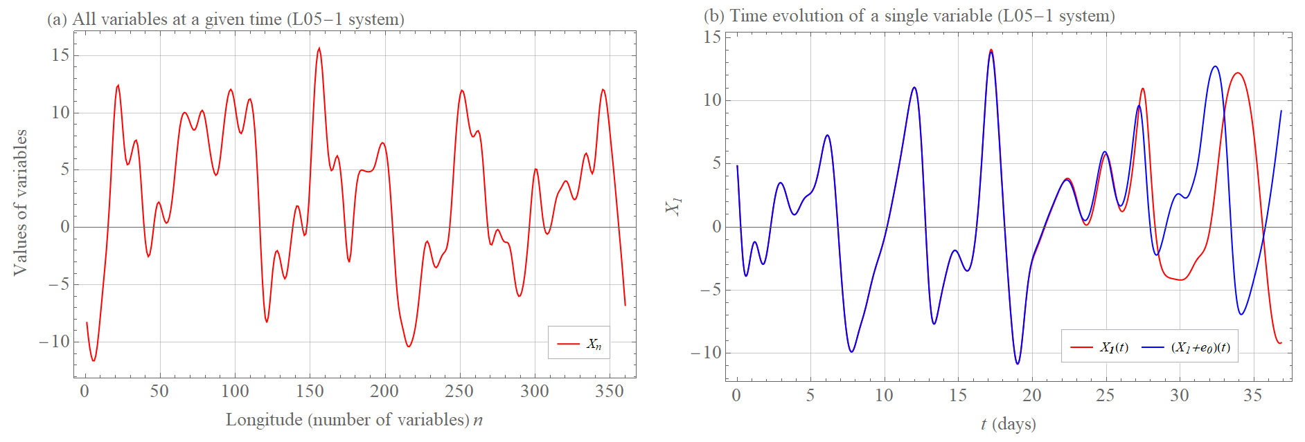
Figure 1 (a) Values of X_n, $n=\mathrm{1},\mathrm{\dots },\mathrm{360}$ variables (red curve) of the L05-1 system at a given time (see Appendix A for more information on the system and its settings). (b) The time evolution t of the variable X₁(t) (red curve) and the time evolution of the initially nearby trajectory (X₁(0)+e₀)(t) (blue curve) of the system L05-1, where e₀=0.01.

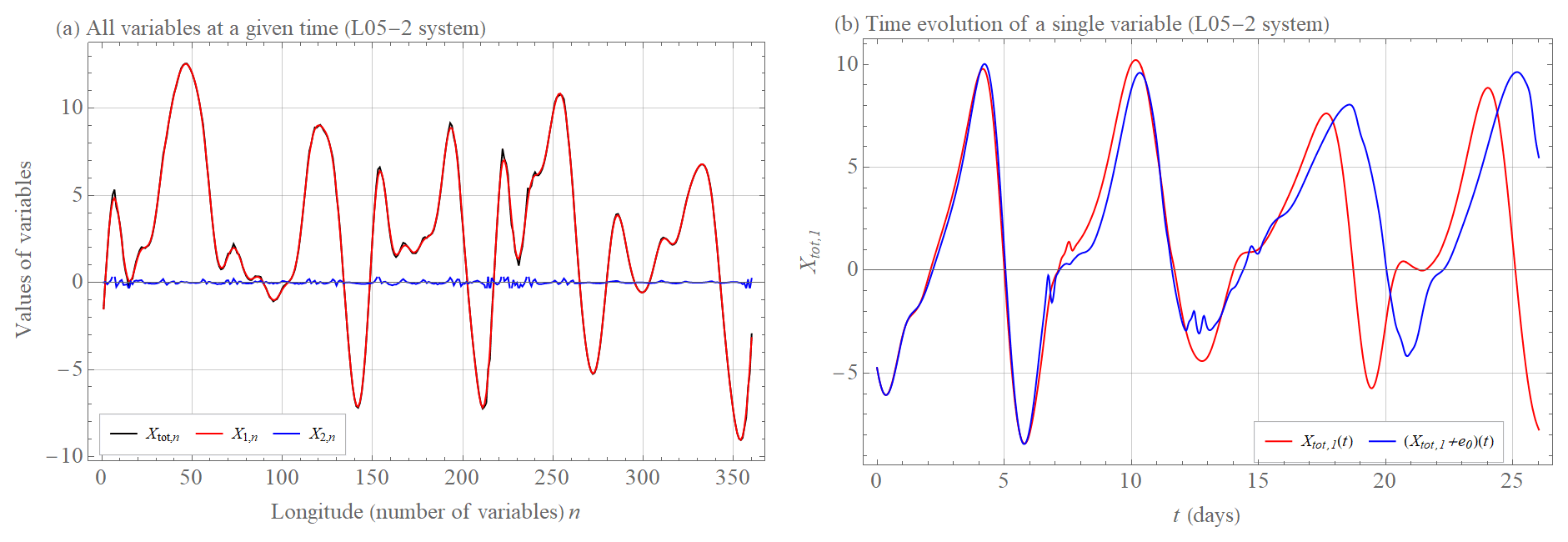
Figure 2 (a) Values of X_1,n (large scale, red curve), X_2,n (small scale, blue curve), and X_tot,n (overall curve, black curve) $n=\mathrm{1},\mathrm{\dots },\mathrm{360}$ variables of the L05-2 system at a given time (see Appendix A for more information on the system and its settings). (b) The time evolution t of the variable X_tot,1(t) (red curve) and the time evolution of the initially nearby trajectory $\left(X_{\text{tot},\mathrm{1}}\right(\mathrm{0})+e_{\mathrm{0}})\left(t\right)$ (blue curve) of the system L05-2, where e₀=0.01.

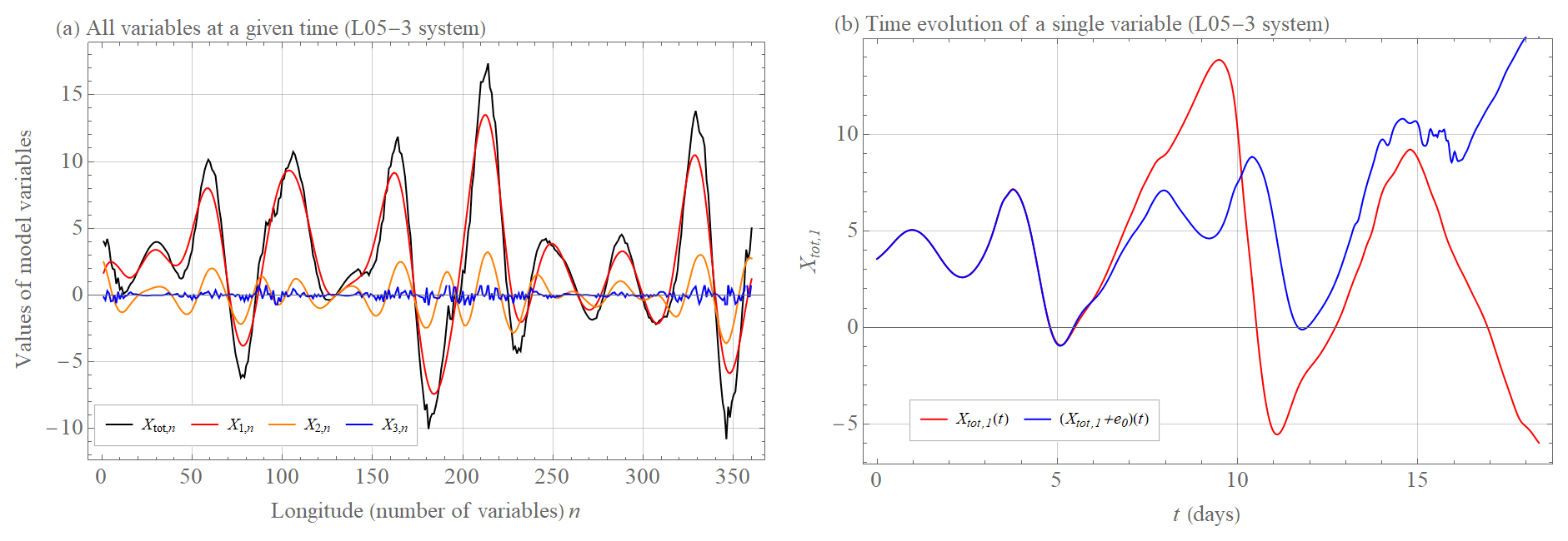
Figure 3 (a) Values of X_1,n (large scale, red curve), X_2,n (medium scale, yellow curve), X_3,n (small scale, blue curve), and X_tot,n (overall curve, black curve) $n=\mathrm{1},\mathrm{\dots },\mathrm{360}$ variables of the L05-3 system at a given time (see Appendix A for more information on the system and its settings). (b) The time evolution t of the variable X_tot,1(t) (red curve) and the time evolution of the initially nearby trajectory $\left(X_{\text{tot},\mathrm{1}}\right(\mathrm{0})+e_{\mathrm{0}})\left(t\right)$ (blue curve) of the system L05-2, where e₀=0.01.

Including small spatiotemporal scales, i.e., improving the model's spatial and temporal resolution, therefore enhances the instability (error growth rate) with respect to initial condition errors. The question under investigation in this paper is whether omitting small-scale atmospheric phenomena, which contribute little to the final value, will improve the predictability of the resulting value. In other words, how does the average forecast error growth change in a model where small-scale phenomena are omitted but where model errors are therefore introduced, compared to a model where all phenomena are present but the average forecast error growth is scale-dependent.

Buizza (2010), Magnusson and Kallen (2013), or Jacobson (2001) show that improving the model's spatial and temporal resolution will improve the prediction ability, especially for short forecast ranges (Buizza, 2010). However, the cited studies work with models that do not model small spatiotemporal phenomena (they are parameterized) and whose initial condition error magnitude is larger than the magnitude of these phenomena. We have verified the fact that the high-resolution model (that models small scales) is less stable than the low-resolution model (that does not model small scales) against initial condition errors (Bednář and Kantz, 2022; Budanur and Kantz, 2022) and that therefore the issue of omitting small scales has another facet. Our new approach models and omits small spatiotemporal scales using the one- and two-scale Lorenz (2005) system (L05-1 and L05-2) and its three-scale extension (L05-3) introduced before in Bednář and Kantz (2022). The omitted scale is the small scale for the L05-2 system, and the small and medium scale are for the L05-3 system. L05 system definition and further details can be found in Appendix A.

The protocol for how to measure the initial error growth for the L05 systems is defined in Sect. 2.1, and the results are presented and compared in Sect. 3.1. The model error scenario, where the L05-1 system is the model and the L05-2 and L05-3 systems are reality, is defined in Sect. 2.2, and the results are presented and compared in Sect. 3.2. The variant with initial and model error is defined in Sect. 2.3, and the results are presented and compared in Sect. 3.3. The results of different error growth scenarios are compared and discussed in Sect. 3.4. Section 4.1 includes the calculation of the model error (drift) defined in Sect. 2.4 and a hypothesis linking the error so defined with the growth of the average model error determined by the difference between model and reality. The meaning of the model error source β in dE_r of Eq. (5) and dE_q Eq. (6) and how to link the value of β with the value of the model error (drift) is discussed and explained in Sect. 4.2. Section 5 presents a similar analysis for the ECMWF forecast system data. Conclusions and discussions are then presented in the final section.

2 Error growth in the L05 systems – types and methods of calculation

The average error magnitude for L05 systems is calculated numerically using the method introduced by Lorenz (1996, 2005). Generally, we define an “error” as the distance between two trajectories where one, the reference trajectory, is supposed to be the “truth”, while a second trajectory is generated under perturbation of the initial condition, under perturbation of the dynamical equations, or both. We measure the error magnitude e(t) after fixed time intervals. We then calculate the mean error magnitude E(t) after fixed times, calculate the average growth tendency $\frac{\mathrm{d}E}{\mathrm{d}t}$ during the last time interval, and report the mean error magnitudes vs. time and the mean growth tendencies (rates) vs. mean error magnitudes.

An alternative method for calculating scale-dependent error growth is called the “finite-size Lyapunov exponent” (Aurell et al., 1996, 1997; Boffetta et al., 1998; Cencini and Vulpiani, 2013). In brief, a finite-size Lyapunov exponent $\mathit{\lambda }=(\mathrm{1}/E)(\mathrm{d}E/\mathrm{d}t)$ or finite-size error growth tendency $\mathrm{d}E/\mathrm{d}t$ can be defined as the ergodic average over phase space of the growth rate of perturbations of a given magnitude E, where the growth rate is defined as the inverse of the time t_f needed for the error magnitude to increase by a pre-defined factor f, hence $\mathit{\lambda }\left(E\right)=(\mathrm{1}/t_f)\ln f$. We choose the former method because it is closer to the process of calculating the average forecast error magnitude of numerical weather prediction systems (Lorenz, 1982; Savijarvi, 1995; Froude et al., 2013; Zhang et al., 2019) and because it is more consistent with the performance of forecasts.

For numerical weather prediction systems, errors in initial conditions and model errors (inaccurate representation of atmospheric processes by the model) are sources of prediction inaccuracy. For the L05 systems, we simulate the initial error growth (perfect model assumption), the model error growth (perfect initial conditions assumption), a combination of both (initial and model error assumption), and the model error growth as defined by Orrell et al. (2001) (drift assumption). To calculate the average error magnitude, a reference trajectory (considered the truth or verification) and a trajectory that is the numerical solution of the systems with a given error are repeatedly generated. For this scheme to be meaningful, we have to ensure that the reference trajectory is on the system's attractor and that the repetition of this scheme samples the whole attractor with correct weights (the invariant measure). We solve this issue in the following way: we first integrate the system over 10 years (175 200 steps), starting from arbitrary initial conditions, and assume that after discarding this transient that the trajectory is on the attractor. We continue to integrate this single trajectory and consider segments of it as reference trajectories for error growth, i.e., the many reference trajectories are simply segments of one very long trajectory, which ensures not only that all these segments are located on the attractor but also that they sample the attractor according to the invariant measure.

2.1 Initial error growth

When we use the term “initial error growth”, we denote the growth of errors in the initial conditions, which limit predictability if a system is chaotic. In order to numerically determine the largest Lyapunov exponent, we have to ensure that initial perturbations already point into the locally most unstable direction since otherwise errors might even shrink over short time periods (this is also a relevant issue in ensemble forecasts, and there its solution is found using bred vectors; see Toth and Kalnay, 1997). We solve these issues in the following way: we start with a random perturbation of the reference trajectory of very small amplitude and let this trajectory evolve over time before determining its distance toward the reference trajectory. In other words, we discard some initial time interval of error growth since this is affected by some transient behavior before it starts to grow with the maximum Lyapunov exponent.

We calculate the initial error growth in systems with one (L05-1), two (L05-2), and three (L05-3) scales to illustrate the behavior in systems with a different number of spatiotemporal scales. The three spatial scales X₁, X₂, and X₃ for the L05-3 system and two spatial scales X₁ and X₂ for the L05-2 system cannot be separated in terms of a coordinate transform but are intrinsically coupled and superimposed in the variables X_tot of the system. The initial conditions of the reality for L05-3 and L05-2 systems are called $X_{\text{tot},\mathrm{0},n}$, from which one finds $X_{\mathrm{1},\mathrm{0},n}$, $X_{\mathrm{2},\mathrm{0},n}$, and $X_{\mathrm{3},\mathrm{0},n}$ through Eqs. (A10), (A11), and (A12), respectively, for the L05-3 system and $X_{\mathrm{1},\mathrm{0},n}$ and $X_{\mathrm{2},\mathrm{0},n}$ through Eqs. (A4) and (A5), respectively, for the L05-2 system. The initial conditions of the reality for the L05-1 system are called X_0,n. The initial values of the “prediction” are then for the L05-1 system $X_{\mathrm{0},n}^{\prime }=X_{\mathrm{0},n}+e_n\left(\mathrm{0}\right)$, where e_n(0) are the initial errors randomly selected from the normal distribution $\text{ND}(\mathit{\mu }=\mathrm{0};\mathit{\sigma }=\mathrm{0.01})$. Since the system's state X_tot is the sum over all spatiotemporal components, for L05-3 and L05-2 systems any arbitrary but small error with spatially uncorrelated components affects only the smallest-scale component. Only a spatially correlated initial error would appear in another component. However, since this error would immediately propagate into the small-scale variables and then grow fastest in these, a perturbation with initial errors in the smallest-scale component is the only practical choice. The initial values of the prediction for the L05-3 system are then $X_{\text{tot},\mathrm{0},n}^{\prime }=X_{\mathrm{1},\mathrm{0},n}+X_{\mathrm{2},\mathrm{0},n}+X_{\mathrm{3},\mathrm{0},n}+e_{\mathrm{3},n}=X_{\text{tot},\mathrm{0},n}+e_{\mathrm{3},n}$, where e_3,n(0) is the initial error randomly selected from the normal distribution $\text{ND}(\mathit{\mu }=\mathrm{0};\mathit{\sigma }=\mathrm{0.001})$. The initial error e_2,n(0) of the L05-2 system is also randomly selected from the same normal distribution, where the initial value of the prediction is $X_{\text{tot},\mathrm{0},n}^{\prime }=X_{\mathrm{1},\mathrm{0},n}+X_{\mathrm{2},\mathrm{0},n}+e_{\mathrm{2},n}=X_{\text{tot},\mathrm{0},n}+e_{\mathrm{2},n}$.

From the initial values of reality and prediction, we integrate the L05 system equations (Eqs. A1, A8, and A9) for 41.7 d (K=2000 steps). In each time step, k of the numerical integration $X_{\mathit{\tau },k,n}$ and $X_{\mathit{\tau },k,n}^{\prime }$ are obtained. The size of the error at a given time kΔt is $e_{\mathit{\tau },n}(k\cdot \mathrm{\Delta }t)=X_{\mathit{\tau },k,n}^{\prime }-X_{\mathit{\tau },k,n}$, where $k=\mathrm{1},\mathrm{\dots },K$, $n=\mathrm{1},\mathrm{\dots },N$ (N=360 variables for all used systems). τ defines a scale or sum of scales ($\mathit{\tau }=\text{tot},\mathrm{1},\mathrm{2},\mathrm{3}$ (L05-3 system), $\mathit{\tau }=\text{tot},\mathrm{1},\mathrm{2}$ (L05-2 system)) and is therefore omitted for the L05-1 system. We perform M=400 runs to calculate the average error growth. In each new run, the initial values $X_{\mathit{\tau },\mathrm{0},n}$ are the last values $X_{\mathit{\tau },K,n}$ of the previous run. The average initial error growth E(t) is calculated as the geometric mean of the runs of the Euclidean distances between reality and prediction:

$$\begin{array}{}\text{(11)}& E_{\text{tot}}(k\cdot \mathrm{\Delta }t)=\sqrt[\mathrm{2}M]{\prod _{m=\mathrm{1}}^M\left({\displaystyle \frac{\mathrm{1}}{N}}\sum _{n=\mathrm{1}}^N{e}_{\mathit{\tau },n,m}^{\mathrm{2}}(k\cdot \mathrm{\Delta }t)\right)}.\end{array}$$

The geometric mean is chosen because of its suitability for comparison with growth governed by the largest Lyapunov exponent. For further information, see Bednář et al. (2014) or Ding and Li (2011). As a result, we have numerical averages for the error growth as a function of time steps after perturbing the reference trajectories in the full phase space and for each scale. We can convert these results into the error growth tendency (rate) as a function of the error magnitude.

2.2 Model error growth

By “model error growth”, we denote the growth of errors caused by the inaccurate description of reality by the “model”. This inaccuracy involves small-scale atmospheric processes unresolved by the model, which for numerical weather prediction systems are approximated to the resolved scale by a procedure called parameterization. It also denotes model biases that are either unknown or have not yet been addressed (Allen et al., 2006). It is a common expectation that model errors in numerical weather forecasts can be reduced by improving the spatial and temporal resolution of the forecast system.

To simulate this in the L05 systems environment (Appendix A), we use the L05-2 and L05-3 systems as the reality and the L05-1 system as the model. Thus, the unresolved or unknown scale is the small scale for the L05-2 system and the small and medium scale for the L05-3 system. This approach is justified by the fact that the L05-2 and L05-3 systems can be viewed as a variant of the L05-1 system:

$$\begin{array}{}\text{(12)}& \mathrm{d}{X}_{\text{tot},n}/\mathrm{d}t=[X_{\mathrm{1}},X_{\mathrm{1}}{]}_{L,n}-X_{\mathrm{1},n}+{\stackrel{\mathrm{̃}}{F}}_n(t),\end{array}$$

where ${\stackrel{\mathrm{̃}}{F}}_n\left(t\right)=b^{\mathrm{2}}[X_{\mathrm{2}},X_{\mathrm{2}}{]}_{\mathrm{1},n}+c[X_{\mathrm{2}},X_{\mathrm{1}}{]}_{\mathrm{1},n}-b{X}_{\mathrm{2},n}+F$ for the L05-2 system and ${\stackrel{\mathrm{̃}}{F}}_n\left(t\right)=b_{\mathrm{1}}^{\mathrm{2}}[X_{\mathrm{2}},X_{\mathrm{2}}{]}_{\mathrm{1},n}+b_{\mathrm{2}}^{\mathrm{2}}[X_{\mathrm{3}},X_{\mathrm{3}}{]}_{\mathrm{1},n}+c_{\mathrm{1}}[X_{\mathrm{2}},X_{\mathrm{1}}{]}_{\mathrm{1},n}+c_{\mathrm{2}}[X_{\mathrm{3}},X_{\mathrm{2}}{]}_{\mathrm{1},n}-b_{\mathrm{1}}{X}_{\mathrm{2},n}-b_{\mathrm{2}}{X}_{\mathrm{3},n}+F$ for the L05-3 system are treated as a forcing, which varies in a complicated manner with time. We parameterize these small-scale phenomena contained in ${\stackrel{\mathrm{̃}}{F}}_n\left(t\right)$ by the average value of these phenomena, which is close to zero, and therefore we can write:

$$\begin{array}{}\text{(13)}& \langle {\stackrel{\mathrm{̃}}{F}}_n\left(t\right)\rangle \approx F=\mathrm{15},\end{array}$$

where 〈…〉 represents the mean calculated over a long orbit on the L05-2 and L05-3 system attractors.

To calculate the average model error growth, we first define initial conditions that are the same for model and reality (perfect initial conditions assumption) and are determined from the values $X_{\text{tot},\mathrm{0},n}$ of reality (L05-2 or L05-3 systems) at the end of the initial transient. Let us stress that we can use $X_{\text{tot},\mathrm{0},n}$ of our high-resolution L05-3 or L05-2 system without any projection as the initial state of the L05-1 system and that the lack of smaller scales is only expressed by the lack of feedback from the smaller scales in the equation of motion.

From these initial values, we integrate the L05-2 or L05-3 system equations (reality) and the L05-1 system equations (model) forward for 41.7 d (K=2000 steps). In each time step k of the numerical integration, $X_{\text{tot},k,n}$ (reality) and X_k,n (model) are obtained. The size of the error at a given time kΔt is $e_{M,n}(k\cdot \mathrm{\Delta }t)=X_{\text{tot},k,n}-X_{k,n}$, where $k=\mathrm{1},\mathrm{\dots },K$, $n=\mathrm{1},\mathrm{\dots },N$ (N=360 variables for all used systems). We perform L=400 runs to calculate the average error growth. In each new run, the initial values $X_{\text{tot},\mathrm{0},n}$ are the last values $X_{\text{tot},K,n}$ of the previous run. The average model error growth E_M(t) is calculated as the geometric mean of the runs of the Euclidean distances between reality and model:

$$\begin{array}{}\text{(14)}& E_M(k\cdot \mathrm{\Delta }t)=\sqrt[\mathrm{2}L]{\prod _{l=\mathrm{1}}^L\left({\displaystyle \frac{\mathrm{1}}{N}}\sum _{n=\mathrm{1}}^N{e}_{M,n,l}^{\mathrm{2}}(k\cdot \mathrm{\Delta }t)\right)}.\end{array}$$

As a result, we have numerical averages for the model error growth as a function of time steps. Note that in this framework, only $X_{\text{tot},k,n}$ (L05-2 and L05-3 systems) values compared to X_k,n (the L05-1 system) and not the individual scales. We can convert these results into the error growth tendency (rate) as a function of the error magnitude.

2.3 Initial and model error growth

By “initial and model error growth”, we denote the combination of the initial error growth defined in Sect. 2.1 and the model error growth defined in Sect. 2.2. We describe the L05-2 and L05-3 systems as reality and the L05-1 system with perturbations in the initial conditions of reality as “model prediction”.

In this setting, we do not discard the initial time interval of initial error growth because this transition period is negligible compared to the model error growth. The initial conditions of the reality for L05-3 and L05-2 systems are called $X_{\text{tot},\mathrm{0},n}$ and determined in the same way described above. The initial values of the model prediction for the L05-1 system are then $X_{\mathrm{0},n}^{\prime }=X_{\text{tot},\mathrm{0},n}+e_n\left(\mathrm{0}\right)$, where e_n(0) values are the initial errors randomly selected from the normal distributions $\text{ND}(\mathit{\mu }=\mathrm{0};\mathit{\sigma }=\mathrm{0.01})$ and $\text{ND}(\mathit{\mu }=\mathrm{0};\mathit{\sigma }=\mathrm{0.2})$. From initial values, we integrate the L05-2 or L05-3 system equations (reality) and the L05-1 system equations (model prediction) forward for 41.7 d (K=2000 steps). In each time step k of the numerical integration, $X_{\text{tot},k,n}$ (reality) and $X_{k,n}^{\prime }$ (model prediction) are obtained. The size of the error at a given time kΔt is $e_{M+\text{ie},n}(k\cdot \mathrm{\Delta }t)=X_{\text{tot},k,n}-X_{k,n}^{\prime }$, where $k=\mathrm{1},\mathrm{\dots },K$, $n=\mathrm{1},\mathrm{\dots },N$ (N=360 variables for all used systems). We perform L=400 runs to calculate the average error growth. In each new run, the initial values $X_{\text{tot},\mathrm{0},n}$ are the last values $X_{\text{tot},K,n}$ of the previous run. The average initial and model error growth E_M+ie(t) is calculated as the geometric mean of the runs of the Euclidean distances between reality and model prediction:

$$\begin{array}{}\text{(15)}& E_{M+\text{ie}}(k\cdot \mathrm{\Delta }t)=\sqrt[\mathrm{2}L]{\prod _{l=\mathrm{1}}^L\left({\displaystyle \frac{\mathrm{1}}{N}}\sum _{n=\mathrm{1}}^N{e}_{M+\text{ie},n,l}^{\mathrm{2}}(k\cdot \mathrm{\Delta }t)\right)}.\end{array}$$

As a result, we have numerical averages for the initial and model error growth as a function of time steps. Note that in this framework only $X_{\text{tot},k,n}$ (L05-2 and L05-3 systems) values are compared to X_k,n (the L05-1 system) and not the individual scales. We can convert these results into the error growth tendency (rate) as a function of the error magnitude.

2.4 Drift

Section 2.2 describes how we can numerically measure the effects of the model error on forecast accuracy. However, if we want to understand how the model error drives the model trajectory away from reality, we need an additional concept. The reason is that model errors at different positions along the trajectory are only weakly correlated. This is a consequence of the fact that the lack of small scales and fast degrees of freedom in the model equations dominates model errors. However, if model errors at different positions along a trajectory are uncorrelated, then they can partially compensate each other, and their effect is not the same as if we assume that model errors along a trajectory are about the same everywhere. Therefore, We will recall the concept of drift as discussed by Orrell et al. (2001). For these purposes, let us first generally define the model (L05-1 system in our case) as $\mathrm{d}\mathit{X}\left(t\right)/\mathrm{d}t=\mathit{G}\left(\mathit{X}\right(t\left)\right)$, where X∈ℝⁿ is the model state space vector (n=360 in our case) and the reality state space vector is $\stackrel{\mathrm{̃}}{\mathit{X}}\left(t\right)\in {\mathbb{R}}^{\stackrel{\mathrm{̃}}{n}}$. In general, $\stackrel{\mathrm{̃}}{n}\ne n$, and it is necessary to project $\stackrel{\mathrm{̃}}{\mathit{X}}$ from the state space of reality to the state space of model (Data Assimilation for Numerical Prediction Models). In our case, $\stackrel{\mathrm{̃}}{n}=n=\mathrm{360}$, $\stackrel{\mathrm{̃}}{\mathit{X}}={\mathit{X}}_{\text{tot}}$, and we use either the L05-2 system $\mathrm{d}{\mathit{X}}_{\text{tot}}\left(t\right)/\mathrm{d}t=\stackrel{\mathrm{̃}}{\mathit{G}}\left({\mathit{X}}_{\mathrm{1}}\right(t),{\mathit{X}}_{\mathrm{2}}(t\left)\right)$ or the L05-3 system $\mathrm{d}{\mathit{X}}_{\text{tot}}\left(t\right)/\mathrm{d}t=\stackrel{\mathrm{̃}}{\mathit{G}}\left({\mathit{X}}_{\mathrm{1}}\right(t),{\mathit{X}}_{\mathrm{2}}(t),{\mathit{X}}_{\mathrm{3}}(t\left)\right)$ as reality. The model error G_e at the point X_tot(t) is then the difference between the model vector field (tendency) and the tendency of the projection of reality into the model space. In our case, we can write the following equation:

$$\begin{array}{}\text{(16)}& {\mathit{G}}_{\mathrm{e}}\left({\mathit{X}}_{\text{tot}}\right(t\left)\right)=\mathit{G}\left({\mathit{X}}_{\text{tot}}\right(t\left)\right)-{\displaystyle \frac{\mathrm{d}{\mathit{X}}_{\text{tot}}\left(t\right)}{\mathrm{d}t}}.\end{array}$$

The drift vector d(τ) was introduced by Orrell et al. (2001) as

$$\begin{array}{}\text{(17)}& {\displaystyle }\begin{array}{rl}{\displaystyle }\mathit{d}\left(\mathit{\tau }\right)& {\displaystyle }={\int }_{\mathrm{0}}^{\mathit{\tau }}{\mathit{G}}_{\mathrm{e}}\left({\mathit{X}}_{\text{tot}}\right(t\left)\right)\mathrm{d}t\\ {\displaystyle }& {\displaystyle }={\int }_{\mathrm{0}}^{\mathit{\tau }}\mathit{G}\left({\mathit{X}}_{\text{tot}}\right(t\left)\right)\mathrm{d}t-{\mathit{X}}_{\text{tot}}\left(\mathit{\tau }\right)+{\mathit{X}}_{\text{tot}}\left(\mathrm{0}\right).\end{array}\end{array}$$

This is an accumulation of model errors along a piece of the model trajectory. As we will see in numerical simulations (Fig. 11), the absolute value of drift |d(τ)| will not grow approximately linearly in time, i.e., it is not the same as accumulating the absolute value of the model error |G_e| along the same piece of the trajectory.

This is a consequence of the here-considered case of neglected small-scale motion: since the ignored scales fluctuate quickly, the model errors at successive positions on the trajectory lose their correlations. We checked this for our L05 models explicitly by calculating the auto-correlation function of the drift vectors as a function of their time lag and found a very fast decay within a few time steps. Therefore, different from model errors in low-dimensional systems, which can be assumed to be spatially highly correlated, one here accumulates random vectors, and the drift therefore follows a path that resembles a Brownian path, as already suggested in Orrel et al. (2001). There and in Orrell (2002) it is also shown how to approximate the integral by summing a series of short-time model errors over finite time steps Δt. The absolute value of drift |d(τ)| as a function of τ grows sublinearly, as will be demonstrated later, which gives a more realistic estimate of the role of model errors. What, however, is ignored here is that a model error in the first time step creates a kind of initial condition error for the second time step, which would then grow as an initial condition error. We will discuss this later.

To calculate the average drift D comparable to previous cases, we first calculate the time evolution of reality $X_{\text{tot},k,n}$ (L05-2 or L05-3 systems), calculated from the initial conditions after the transient period. From each time step k of the time evolution of $X_{\text{tot},k,n}$ reality (up to K=2000 steps), we calculate the one-step Δt time evolution of the model. $X_{\text{tot},k,n}=X_{k,n}$ values are therefore viewed as initial conditions for the one-step Δt time evolution of the model. The size of the drift at a given time kΔt is the sum of all previous and current error vectors: ${\mathit{d}}_n(k\cdot \mathrm{\Delta }t)={\sum }_{j=\mathrm{0}}^{k-\mathrm{1}}\left({\mathit{X}}_{j,n}\right((j+\mathrm{1})\cdot \mathrm{\Delta }t)-{\mathit{X}}_{\text{tot},j+\mathrm{1},n})$, where $k=\mathrm{1},\mathrm{\dots },K$, $n=\mathrm{1},\mathrm{\dots },N$ (N=360 variables for all used systems). Notice that it is not the absolute values of the Δt errors that are accumulated but the vectors (see Fig. 4), meaning that in the summation there can be cancellation effects and hence a slower-than-linear growth of the drift with time.

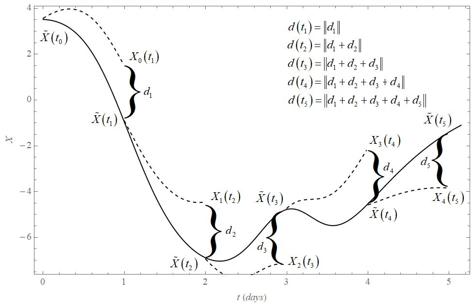
Figure 4 Schematic description of drift d calculation. The solid curve shows the time evolution of the reality projected into the model space $\stackrel{\mathrm{̃}}{X}\left(t_j\right)$ at the time $t_j=j\cdot \mathrm{\Delta }t$ for $j=\mathrm{1},\mathrm{\dots },\mathrm{5}$. The dashed curves show the short (Δt) time evolutions of the model X_j(t) for t≥t_j initiated at the points $\stackrel{\mathrm{̃}}{X}\left(t_j\right)$. Drift d(t) is then the sum of the difference $d\left(t_{j+\mathrm{1}}\right)=X_j\left(t_{j+\mathrm{1}}\right)-\stackrel{\mathrm{̃}}{X}\left(t_{j+\mathrm{1}}\right)$ at each time step.

We perform L=400 runs in order to calculate the average error growth. In each new run, the initial values $X_{\text{tot},\mathrm{0},n}$ are the last values $X_{\text{tot},K,n}$ of the previous run. The average drift D(t) is defined as the geometric mean of the runs of the Euclidean distances between reality and model:

$$\begin{array}{}\text{(18)}& D(k\cdot \mathrm{\Delta }t)=\sqrt[\mathrm{2}L]{\prod _{l=\mathrm{1}}^L\left({\displaystyle \frac{\mathrm{1}}{N}}\sum _{n=\mathrm{1}}^N{d}_{n,l}^{\mathrm{2}}(k\cdot \mathrm{\Delta }t)\right)}.\end{array}$$

As a result, we have numerical averages for the drift as a function of time step. We can convert these results into the drift growth tendency as a function of the drift magnitude.

3 Error growth in the L05 systems – results and comparisons

Based on the described methods, we calculate the average prediction error growth for L05 systems. We approximate the numerical error growth curves using the hypotheses Eqs. (1)–(6) and try to identify the most appropriate description. We use these results to determine how the average forecast error growth changes in a model where small-scale phenomena are omitted, but the model error is therefore created (perfect initial conditions assumption or initial and model error assumption) compared to a model where all phenomena are present, whereas the average forecast error growth is scale-dependent (perfect model assumption). The resulting behavior will be explained using the drift.

3.1 Initial error growth

Figure 5a shows the initial error growth rate (tendency) $\mathrm{d}E/\mathrm{d}t$ as a function of the error magnitude E for the L05-1 system, while Fig. 5b shows the error magnitude as a function of time. We also show the best-fit results of the error growth models represented by Eqs. (1)–(6). It turns out that the initial part of the growth rate is linear without any significant offset, i.e., we see a linear increase with a beginning at ($E=\mathrm{0},\mathrm{d}E/\mathrm{d}t=\mathrm{0}$). Therefore, constants in the error growth models that were included to represent the model error are consequently close to zero. In addition, the power law fit yields a power close to 1. Because of the saturation of the error after some time, the error growth rate decays to zero when the error is large, which can be represented well by the factor ($\mathrm{1}-E/E_{\text{lim}}$) in the error growth models. Hence, all models with this saturation term allow good fits to the error growth rate and the error magnitude as a function of time in the whole range and confirm that the L05-1 system is a classical chaotic system with the largest Lyapunov exponent of about λ≈0.33 d⁻¹.

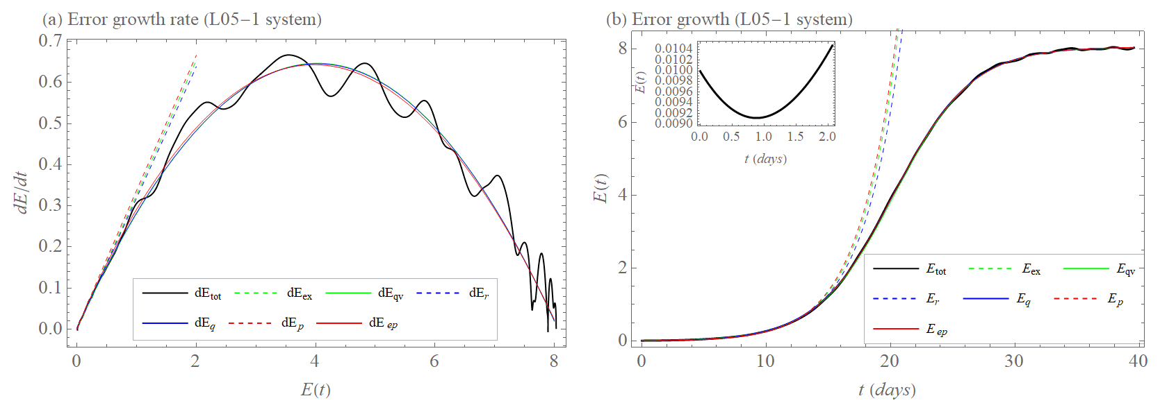
Figure 5 (a) Initial error growth tendency (rate) $\mathrm{d}E/\mathrm{d}t$ as a function of the error magnitude E (dE_tot, black). Approximation of the early part of the growth by exponential growth rate dE_ex (Eq. 1, dashed green); exponential growth rate with model error dE_r (Eq. 5, dashed blue) and power law dE_p (Eq. 3, dashed red). Approximation of the full curve by growth rate of quadratic hypothesis dE_qv (Eq. 2, green); growth rate of quadratic hypothesis with model error dE_q (Eq. 6, blue); and extended power law dE_ep (Eq. 4, red) for the L05-1 system. (b) Initial error growth E as a function of time t (E_tot, Eq. 11, black). Approximation of the early part of the growth by integration of dE_ex (E_ex, dashed green) with λ_ex=0.33 d⁻¹; integration of dE_r (E_r, dashed blue) with λ_r=0.32 d⁻¹ and β_r=0.00006 unit d⁻¹; integrations of dE_p (E_p, dashed red) with a=0.34 unit^0.02 d⁻¹ and b=0.02. Approximation of the full curve by integration of dE_qv (E_qv, green) with λ_qv=0.32 d⁻¹ and E_lim=8.1 unit; integration of dE_q (E_q, blue) with λ_q=0.32 d⁻¹, β_q=0.003 unit d⁻¹ and E_lim=8.1 unit; and integration of dE_ep (E_ep, red) with a=0.33 unit^0.03 d⁻¹, b=0.03, and E_lim=8.1 unit for the L05-1 system. The inset shows transient behavior before the error magnitude grows (for more details, see Sect. 2.1).

The behavior is obviously different for the L05-2 system, which contains additional small-scale degrees of freedom, as shown in Fig. 6. The initial part of the error growth rate (for small E) is already curved, and hence the exponential growth model does not provide a good fit anymore. Introducing a non-vanishing error growth rate right from the beginning, i.e., starting from ($E=\mathrm{0},\mathrm{d}E/\mathrm{d}t={\mathit{\beta }}_{\mathrm{r}}$), which is the description by dE_r, the approximation moves closer to the data, but this is in clear contradiction to the initial error growth idea. Due to the lack of model errors, the growth rate starts from 0. In addition, the quadratic hypothesis is unable to reproduce this curvature well enough. Therefore, the data are best approximated by the power law in the initial part and by the extended power law with saturation on the whole range.

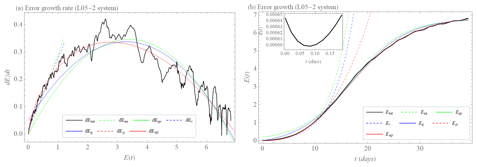
Figure 6 (a) Initial error growth tendency (rate) $\mathrm{d}E/\mathrm{d}t$ as a function of the error magnitude E (dE_tot, black). Approximation of the early part of the growth by exponential growth rate dE_ex (Eq. 1, dashed green); exponential growth rate with model error dE_r (Eq. 5, dashed blue); and power law dE_p (Eq. 3, dashed red). Approximation of the full curve by growth rate of quadratic hypothesis dE_qv (Eq. 2, green); and growth rate of hypothesis with model error dE_q (Eq. 6, blue) and extended power law dE_ep (Eq. 4, red) for the L05-2 system. (b) Initial error growth E as a function of time t (E_tot, Eq. 11, black). Approximation of the early part of the growth by integration of dE_ex (E_ex, dashed green) with λ_ex=0.29 d⁻¹; integration of dE_r (E_r, dashed blue) with λ_r=0.26 d⁻¹ and β_r=0.02 unit d⁻¹; integrations of dE_p (E_p, dashed red) with a=0.25 unit^0.32 d⁻¹ and b=0.32. Approximation of the full curve by integration of dE_qv (E_qv, green) with λ_qv=0.2 d⁻¹ and E_lim=6.8 unit; integration of dE_q (E_q, blue) with λ_q=0.18 d⁻¹, β_q=0.05 unit d⁻¹, and E_lim=6.8 unit and integration of dE_ep (E_ep, red) with a=0.28 unit^0.34 d⁻¹, b=0.34 and E_lim=7 unit for the L05-2 system. The inset shows transient behavior before the error magnitude grows (for more details, see Sect. 2.1).

What we found for the initial error growth of the L05-2 system is even more pronounced in the L05-3 system with three spatiotemporal scales. The superiority of approximations dE_p and dE_ep over the other approximations is enhanced by the even faster growth of E_tot(t) compared to the exponential growth and E_tot(t) for the L05-2 system (Fig. 7). The reason for this behavior is described in Brisch and Kantz (2019) or in Bednář and Kantz (2022). Lorenz's (1969) statement can summarize it: a typical quantity to be predicted is a superposition of the dynamics on different scales. After a fast growth of the small-scale errors with saturation at these very same small scales, the large-scale errors continue to grow at a slower rate until even these saturate. This is the phenomenon of scale-dependent error growth. We also see that if we interpret the three systems L05-1 to L05-3 as low- and high-resolution models, the high-resolution model has larger instability and hence a shorter time until an ensemble of initial conditions has spread out on the attractor. If this were of relevance for the prediction horizon, then the high-resolution model would be less useful for forecasting than the low-resolution model.

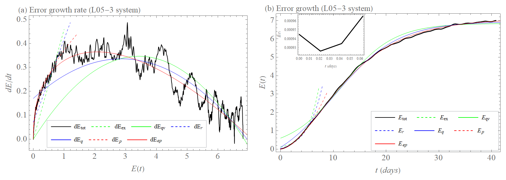
Figure 7 (a) Initial error growth tendency (rate) $\mathrm{d}E/\mathrm{d}t$ as a function of the error magnitude E (dE_tot, black). Approximation of the early part of the growth by exponential growth rate dE_ex (Eq. 1, dashed green); exponential growth rate with model error dE_r (Eq. 5, dashed blue); and power law dE_p (Eq. 3, dashed red). Approximation of the full curve by growth rate of quadratic hypothesis dE_qv (Eq. 2, green); and growth rate of quadratic hypothesis with model error dE_q (Eq. 6, blue) and extended power law dE_ep (Eq. 4, red) for the L05-3 system. (b) Initial error growth E as a function of time t (E_tot, Eq. 11, black). Approximation of the early part of the growth by integration of dE_ex (E_ex, dashed green) with λ_ex=0.46 d⁻¹; integration of dE_r (E_r, dashed blue) with λ_r=0.35 d⁻¹ and β_r=0.07 unit d⁻¹; integrations of dE_p (E_p, dashed red) with a=0.37 unit^0.63 d⁻¹ and b=0.63. Approximation of the full curve by integration of dE_qv (E_qv, green) with λ_qv=0.2 d⁻¹ and E_lim=6.9 unit; integration of dE_q (E_q, blue) with λ_q=0.14 d⁻¹, β_q=0.17 unit d⁻¹, and E_lim=6.9 unit; and integration of dE_ep (E_ep, red) with a=0.38 unit^0.59 d⁻¹, b=0.59, and E_lim=7.1 unit for the L05-3 system. The inset shows transient behavior before the error magnitude grows (for more details, see Sect. 2.1).

3.2 Model error growth

We use the L05-2 system as reality and make forecasts using the L05-1 system. Their suitably averaged differences give rise to the model error as a function of lead time. Figure 8a (solid black curve) shows the model error growth rate $\mathrm{d}E/\mathrm{d}t$ as a function of the error magnitude E, while Fig. 8b shows the time evolution of this error. We see an initially very fast error growth caused by the differences in the equations of motion of reality and the model. After a short transient, we see in both panels of Fig. 8a behavior compatible with our error growth models. Those models with a constant term (i.e., the quadratic hypothesis with model error and the exponential growth with model error) provide the best fits, where to be good in the whole range the factor $(\mathrm{1}-E/E_{\text{lim}})$ of the quadratic hypothesis with model error is needed. In view of what will follow, we stress that based on the data both E_r and E_q provide good fits up to error magnitudes of about three units, with different values λ_q≈0.27 d⁻¹ and λ_r≈0.17 d⁻¹ of the largest Lyapunov exponent.

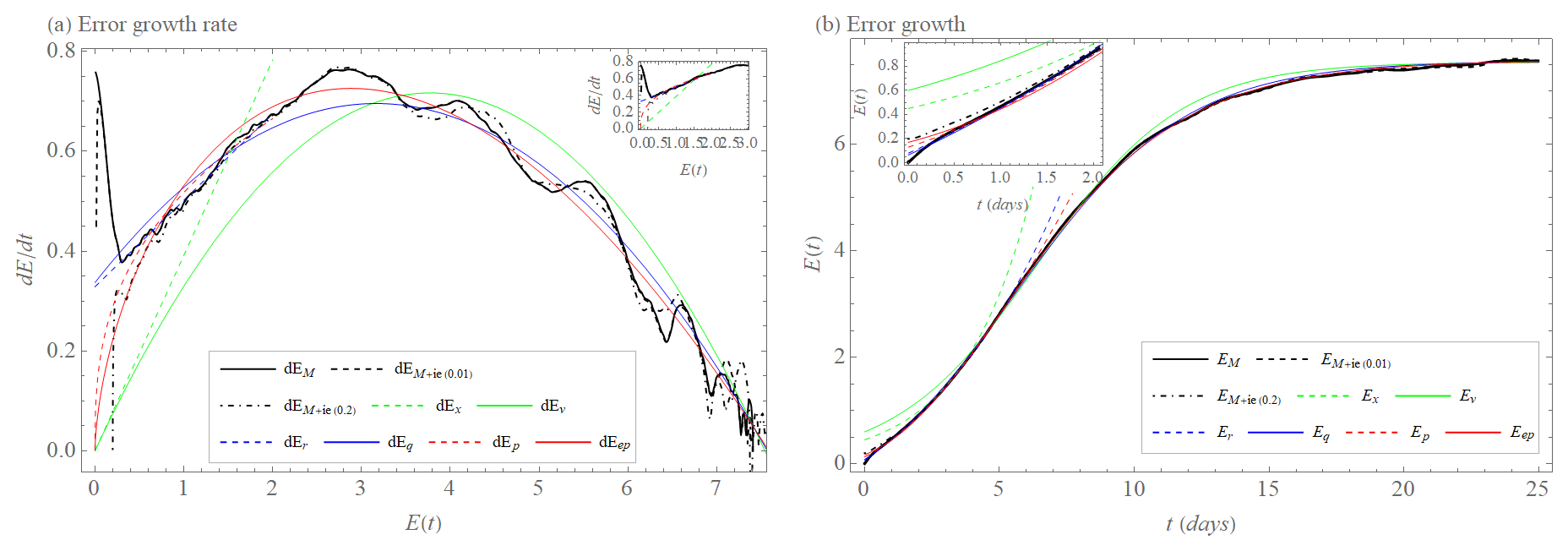
Figure 8 (a) Model error growth tendency (rate) $\mathrm{d}E/\mathrm{d}t$ as a function of the error magnitude E (dE_M, black); initial and model error growth tendency $\mathrm{d}E/\mathrm{d}t$ as a function of the error magnitude E (dE_M+ie(0.01) (dashed black) for E(0)=0.01 and dE_M+ie(0.2) (dashed–dotted black) for E(0)=0.2). Approximation of the early part of the model growth by exponential growth rate dE_ex (Eq. 1, dashed green); exponential growth rate with model error dE_r (Eq. 5, dashed blue) and power law dE_p (Eq. 3, dashed red). Approximation of the full curve by growth rate of quadratic hypothesis dE_qv (Eq. 2, green), growth rate of quadratic hypothesis with model error dE_q (Eq. 6, blue), and extended power law dE_ep (Eq. 4, red) for the L05-2 system as the reality and the L05-1 system as the model. The inset shows the early phase. (b) Model error growth E as a function of time t (E_M, Eq. 14, black); initial and model error growth E as a function of time t (E_M+ie(0.01) (Eq. 15, dashed black), for E(0)=0.01 and E_M+ie(0.2) (Eq. 15, dashed–dotted black) for E(0)=0.2). Approximation of the early part of the growth by integration of dE_ex (E_ex, dashed green) with λ_ex=0.39 d⁻¹; integration of dE_r (E_r, dashed blue) with λ_r=0.17 d⁻¹ and β_r=0.33 unit d⁻¹; integrations of dE_p (E_p, dashed red) with a=0.52 unit^0.64 d⁻¹ and b=0.64. Approximation of the full curve by integration of dE_qv (E_qv, green) with λ_qv=0.38 d⁻¹ and E_lim=7.5 unit, integration of dE_q (E_q, blue) with λ_q=0.27 d⁻¹, β_q=0.34 unit d⁻¹ and E_lim=7.6 unit, and integration of dE_ep (E_ep, red) with a=0.61 unit^0.39 d⁻¹, b=0.39, and E_lim=7.6 unit for the L05-2 system as the reality and the L05-1 system as the model. The inset shows the early phase of the time evolution.

When we use L05-3 as reality and L05-1 as the model, the same conclusions are valid for the model error growth rate $\mathrm{d}E/\mathrm{d}t$ as a function of the error magnitude E (Fig. 9a) and E_M(t) (Fig. 9b). Note, however, that the rates $\mathrm{d}E/\mathrm{d}t\left(E\right)$ have much larger maximal values and that E_M(t) grows faster than when taking L05-2 as reality. However, if we ignore the very initial part of the error growth rate for small values E, which the error growth models cannot reproduce, we see that E_r and E_q provide the best fits.

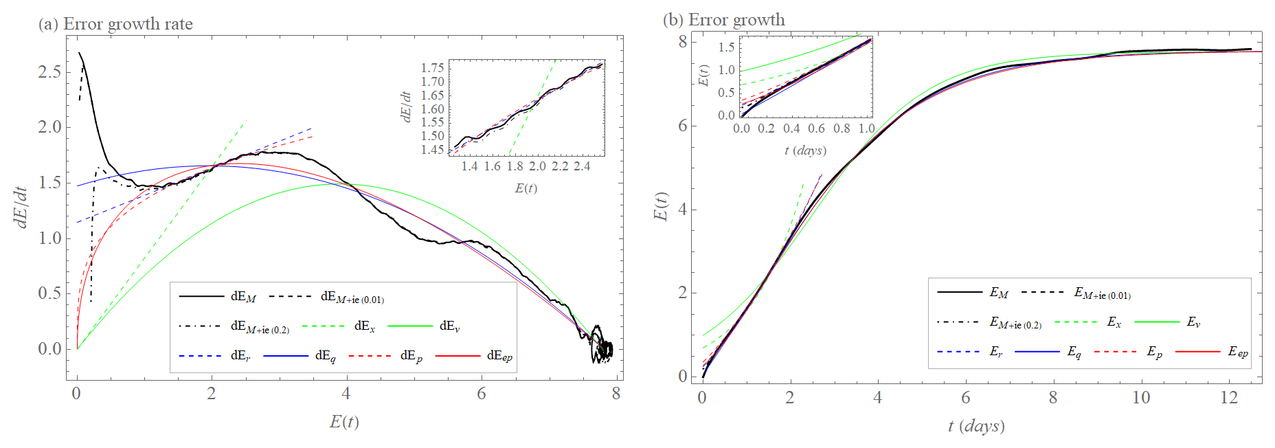
Figure 9 (a) Model error growth tendency (rate) $\mathrm{d}E/\mathrm{d}t$ as a function of the error magnitude E (dE_M, black); initial and model error growth tendency $\mathrm{d}E/\mathrm{d}t$ as a function of the error magnitude E (dE_M+ie(0.01) (dashed black) for E(0)=0.01 and dE_M+ie(0.2) (dashed–dotted black) for E(0)=0.2). Approximation of the early part of the model growth by exponential growth rate dE_ex (Eq. 1, dashed green); exponential growth rate with model error dE_r (Eq. 5, dashed blue), power law dE_p (Eq. 3, dashed red). Approximation of the full curve by growth rate of quadratic hypothesis dE_qv (Eq. 2, green); and growth rate of quadratic hypothesis with model error dE_q (Eq. 6, blue) and extended power law dE_ep (Eq. 4, red) for the L05-3 system as the reality and the L05-1 system as the model. The inset shows the early phase. (b) Model error growth E as a function of time t (E_M, Eq. 14, black); initial and model error growth E as a function of time t (E_M+ie(0.01) (Eq. 15, dashed black) for E(0)=0.01 and E_M+ie(0.2) (Eq. 15, dashed–dotted black) for E(0)=0.2). Approximation of the early part of the growth by integration of dE_ex (E_ex, dashed green) with λ_ex=0.83 d⁻¹, integration of dE_r (E_r, dashed blue) with λ_r=0.25 d⁻¹ and β_r=1.15 unit d⁻¹, integrations of dE_p (E_p, dashed red) with a=1.35 unit^0.72 d⁻¹ and b=0.72. Approximation of the full curve by integration of dE_qv (E_qv, green) with λ_qv=0.77 d⁻¹ and E_lim=7.8 unit, integration of dE_q (E_q, blue) with λ_q=0.38 d⁻¹, β_q=1.47 unit d⁻¹, and E_lim=7.8 unit, and integration of dE_ep (E_ep, red) with a=1.64 unit^0.55 d⁻¹, b=0.55, and E_lim=7.8 unit for the L05-3 system as the reality and the L05-1 system as the model. The inset shows the early phase of the time evolution.

3.3 Initial and model error growth

In both settings, we also show the results when we include a small initial condition error in addition to the model error. This initial condition error implies that the forecast error as a function of time starts with a non-zero value and correspondingly with a much lower growth rate than the model error alone, but apart from that there are no strong effects. Figures 8 and 9 show that it is not the net sum of the initial error growth E_tot(t) and the model error growth E_M(t). E_M+ie(t) goes from the initial value E_M+ie(0) through some transition period to the model error growth curve E_M(t). E_M(t) is therefore the limiting value to which E_M+ie(t) is attracted. Indeed, solid and dashed black curves in the insets of Figs. 8b and 9b show that already after time t=0.2 the model error alone has grown so much that there is no effect of even of the larger initial condition error of magnitude E(0)=0.2 anymore. The larger the initial error and the smaller the model error, the longer the transition period, but it is still short for realistic values of the initial condition error. For these reasons, it can be seen that the appropriate approximation for describing the variant with initial and model error remains the same as for describing the variant with model error only, which is the exponential growth with model error, dE_r Eq. (5), for the early growth phase and the quadratic hypothesis with model error dE_q, Eq. (6), for the entire length of the evolution (Figs. 8 and 9).

3.4 Comparison of initial and model error growth

We want to use the approximation formulae to construct the error curves for E_tot(0)=0, =0.1, and =0.2. The initial error magnitudes of 0.1 and 0.2 correspond to the relative values of the initial errors of current numerical weather prediction models for the L05 models. For the initial error growth E_tot(t) (for simplicity, let us redefine E_tot(t) to E_ie(t)), we use the extended power law solution and find the parameter values $\mathrm{d}{E}_{\text{ep}}=\mathrm{0.28}\cdot E^{\mathrm{0.66}}(\mathrm{1}-E/\mathrm{7})$ for the L05-2 system and $\mathrm{d}{E}_{\text{ep}}=\mathrm{0.38}\cdot E^{\mathrm{0.41}}(\mathrm{1}-E/\mathrm{7.1})$ for the L05-3 system, with initial values E_ie(0)(0)→0 (Fig. 10, solid red curve), E_ie(0.1)(0)=0.1 (Fig. 10a, dashed red curve), and E_ie(0.2)(0)=0.2 (Fig. 10b, dashed red curve).

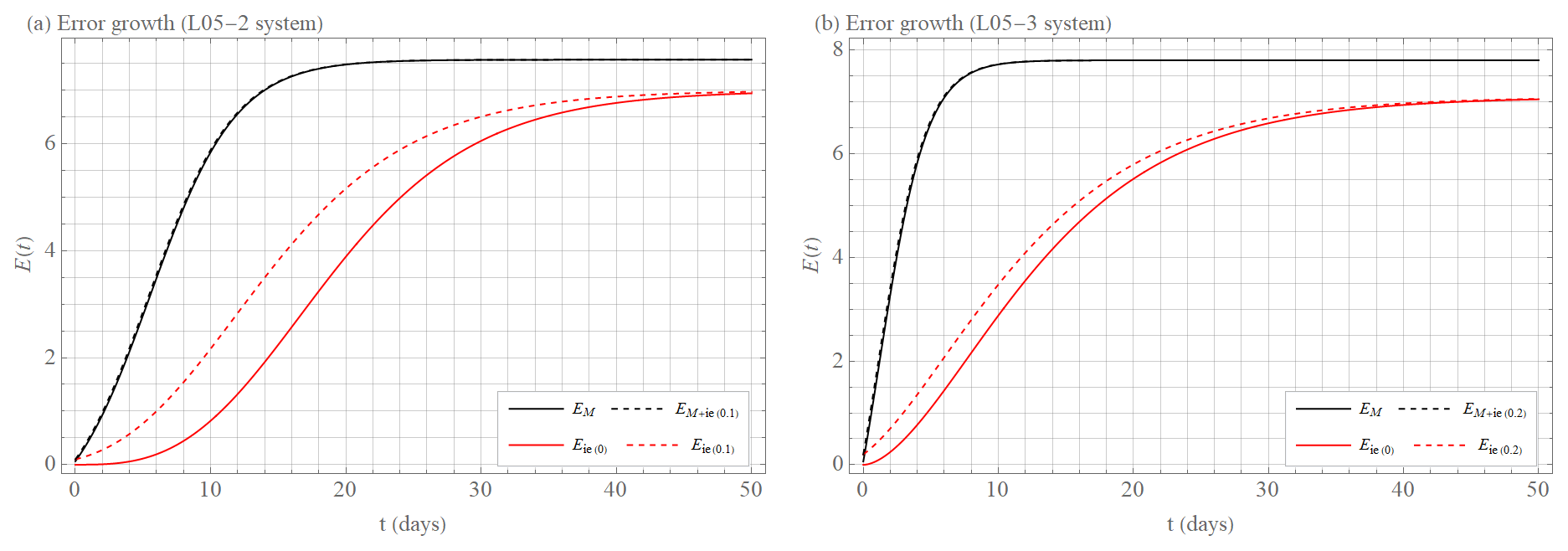
Figure 10 Error growth E as a function of time t. The solid black curve shows model error growth E_M (Eq. 14), the dashed black curve shows initial and model error growth E_M+ie (Eq. 15), the solid red curve displays initial error growth E_ie for E(0)→0 (Eq. 11), and the dashed red curve displays initial error growth E_ie for (a) E(0)≈0.1 and (b) E(0)≈0.2 (Eq. 11). Shown are calculations of the best-fit approximations for given types of error growth (see Sect. 3 for more details). The initial error growth E_ie is calculated for (a) the L05-2 system and (b) the L05-3 system. The model error growth E_M and initial plus the model error growth E_M+ie is calculated as the difference (a) between the L05-1 system and the L05-2 system and (b) between the L05-1 system and the L05-3 system.

For the model error growth E_M(t), we use the quadratic hypothesis with model error with the following best-fit parameters: $\mathrm{d}{E}_{\mathrm{q}}\left(t\right)/\mathrm{d}t=(\mathrm{0.27}\cdot E+\mathrm{0.34})(\mathrm{1}-E/\mathrm{7.6})$ and E_M(0)≈0.1 for the L05-2 system and $\mathrm{d}{E}_{\mathrm{q}}\left(t\right)/\mathrm{d}t=(\mathrm{0.38}\cdot E+\mathrm{1.47})(\mathrm{1}-E/\mathrm{7.8})$ with E_M(0)≈0.1 for the L05-3 system.

The reason why E₀ is non-zero when using the approximation can be found in Sect. 4.2. We can use the same approximations for the initial and model error growth E_M+ie(t) as for the model error growth alone, E_M(t) with $E_{M+\text{ie}\left(\mathrm{0.1}\right)}\left(\mathrm{0}\right)=\mathrm{0.1}$ for the L05-2 system, and $E_{M+\text{ie}\left(\mathrm{0.2}\right)}\left(\mathrm{0}\right)=\mathrm{0.2}$ for the L05-3 system. The justification can be found in Sect. 4.3.

In addition to the graphical representation (Fig. 10), we compare the variants by expressing the times t_95 %, t_71 %, t_50 %, and t_25 % when the error magnitude E reaches 95 %, 71 %, 50 %, and 25 %, respectively, of its limiting (saturated) value E_lim. In the literature, t_95 % is understood as a practical predictability limit, while t_71 % corresponds to climatic variability, according to Savijarvi (1995). For Fig. 10, let us first comment on the difference between the limiting (saturation) values E_lim of the initial error curves E_ie(t) and the model error curves E_M(t) or E_M+ie(t). The pure initial error curves are produced in the perfect model scenario, meaning that forecast and reality are obtained with the same system. When model error is present, the variability of forecast and reality is different, and hence the limiting error is larger, in agreement with Simmons et al. (1995) or Li et al. (2018).

Figure 10 also provides insight into our question of whether high-resolution or low-resolution models will produce better forecasts. We recall that high-resolution models suffer from much faster initial condition error growth due to the stronger instability of small-scale motion. However, the small scales usually do not contribute to the forecast target. Figure 10 shows that predictability is significantly worsened by the model error rather than by the initial error growth. This means that the average forecast error in a model where small-scale phenomena are omitted but the model error is therefore present (black curves E_M(t) and E_M+ie(t)) grows significantly faster compared to a model where all scales are resolved (no model error) but the average forecast error growth is scale-dependent (red curves E_ie(t)). However, this phenomenon depends on the relative magnitudes of the model error term β, the (effective) Lyapunov exponent λ, and the initial condition error. If the growth rate λ were larger and the model error smaller, then the exponential error growth would overwhelm the contribution of model error in every time step. In our numerical experiments using the L05 models, the magnitude of the initial condition error is tuned to values corresponding to initial condition errors in real weather forecasts, so we are tempted to believe that in weather forecasts high-resolution models should also be superior.

Specifically, for the L05-2 system (Fig. 10a), the forecast with model error (i.e., using L05-1 for the forecast), the time t₂₅ is more than 3 times shorter than the limit without model and initial condition error (E_ie(0)(0)→0), being $t_{\mathrm{25}\mathit{\%},M}=\mathrm{4}$ d and $t_{\mathrm{25}\mathit{\%},\text{ie(0)}}=\mathrm{13}$ d, respectively. With increasing error magnitude, the ratio of forecast times decreases ($t_{\mathrm{50}\mathit{\%},M}=\mathrm{6}$ d vs. $t_{\mathrm{50}\mathit{\%},\text{ie(0)}}=\mathrm{19}$ d and $t_{\mathrm{71}\mathit{\%},M}=\mathrm{9}$ d vs. $t_{\mathrm{71}\mathit{\%},\text{ie(0)}}=\mathrm{24}$ d) until $t_{\mathrm{95}\mathit{\%},M}=\mathrm{16}$ d, which is approximately half as large as $t_{\mathrm{95}\mathit{\%},\text{ie(0)}}=\mathrm{37}$ d. Adding the error of the initial condition does not significantly change the error growth for the model error variant ($E_M\left(t\right)\approx E_{M+\text{ie}\left(\mathrm{0.1}\right)}\left(t\right)$; see Sect. 4.3 for details). The error growth naturally increases for the variant with the initial error, and the ratio is reduced to twice the growth rate over the entire growth period ($t_{\mathrm{25}\mathit{\%},M+\text{ie(0.1)}}=\mathrm{4}$ d vs. $t_{\mathrm{25}\mathit{\%},\text{ie(0.1)}}=\mathrm{9}$ d, $t_{\mathrm{50}\mathit{\%},M+\text{ie(0.1)}}=\mathrm{6}$ d vs. $t_{\mathrm{50}\mathit{\%},\text{ie(0.1)}}=\mathrm{14}$ d, $t_{\mathrm{71}\mathit{\%},M+\text{ie(0.1)}}=\mathrm{9}$ d vs. $t_{\mathrm{71}\mathit{\%},\text{ie(0.1)}}=\mathrm{19}$ d, and $t_{\mathrm{95}\mathit{\%},M+\text{ie(0.1)}}=\mathrm{16}$ d vs. $t_{\mathrm{95}\mathit{\%},\text{ie(0.1)}}=\mathrm{32}$ d).

For the L05-3 system (Fig. 10b) taken as truth, the effect is even more dramatic. Without initial error (respectively for E_ie(0)(0)→0), $t_{\mathrm{25}\mathit{\%},M}=\mathrm{1}$ d is 7 times smaller than $t_{\mathrm{25}\mathit{\%},\text{ie(0)}}=\mathrm{7}$ d. Gradually, the ratio decreases ($t_{\mathrm{50}\mathit{\%},M}=\mathrm{2}$ d vs. $t_{\mathrm{50}\mathit{\%},\text{ie(0)}}=\mathrm{12}$ d and $t_{\mathrm{71}\mathit{\%},M}=\mathrm{4}$ d vs. $t_{\mathrm{71}\mathit{\%},\text{ie(0)}}=\mathrm{18}$ d) until $t_{\mathrm{95}\mathit{\%},M}=\mathrm{8}$ d, which is approximately 4 times smaller than $t_{\mathrm{95}\mathit{\%},\text{ie(0)}}=\mathrm{34}$ d. Adding the error of the initial condition does not significantly change the error growth for the model error variant ($E_M\left(t\right)\approx E_{M+\text{ie(0.2)}}\left(t\right)$; see Sect. 4.3 for details). The growth changes for the variant with the initial error, and the ratio is reduced to 5 times the growth rate in the first half of growth ($t_{\mathrm{25}\mathit{\%},M+\text{ie(0.2)}}=\mathrm{1}$ d vs. $t_{\mathrm{25}\mathit{\%},\text{ie(0.2)}}=\mathrm{5}$ d, $t_{\mathrm{50}\mathit{\%},M+\text{ie(0.2)}}=\mathrm{2}$ d vs. $t_{\mathrm{50}\mathit{\%},\text{ie(0.2)}}=\mathrm{10}$ d, $t_{\mathrm{71}\mathit{\%},M+\text{ie(0.2)}}=\mathrm{4}$ d vs. $t_{\mathrm{71}\mathit{\%},\text{ie(0.2)}}=\mathrm{16}$ d, and $t_{\mathrm{95}\mathit{\%},M+\text{ie(0.2)}}=\mathrm{8}$ d vs. $t_{\mathrm{95}\mathit{\%},\text{ie(0.2)}}=\mathrm{34}$ d).

In the numerical error growth study described so far, we used L05-1 as a model and compared its performance to two types of reality with different spatiotemporal resolutions. We complemented this study using as a single reality the L05-3 system and comparing the performance of the L05-1 and L05-2 models when using them for forecasts as two forecasts with different spatiotemporal resolutions. These findings (not shown) confirm the dominance of the model error over the initial condition error growth, i.e., the model with the higher resolution again provides better forecasts even for larger errors and therefore has a better prediction horizon. However, the effect in this setting is not as dramatic as in the results presented above .

4 Error growth in the L05 systems – discussion and explanation of results

In this section, we present considerations that explain the dominance of the model error in our forecast studies, where the notion of the drift (Sect. 2.4) plays a relevant role. We will consider the feedback of the drift as an initial error, which modifies the interpretation of the parameters in the exponential growth with model error dE_r (Eq. 5) and the quadratic hypothesis with model error dE_q (Eq. 6) and its relationship with the drift.

4.1 Drift and its role in explaining the model error growth

Figure 11 compares the model error growth E_M(t) (Eq. 14), the drift D(t) (Eq. 18), and the exponential growth approximation with model error E_r(t) (Eq. 5). The curves are determined from the difference between the L05-2 and the L05-1 systems (Fig. 11a) and between the L05-3 and the L05-1 systems (Fig. 11b) for error magnitudes where the saturation effect is not yet present (up to 2 and 3 d). We intend to understand the behavior of the model error since this is the issue in real forecasts. The drift D(t) (Fig. 11, blue curve) describes the early part of the model error evolution E_M(t) (Fig. 11, black curve) very well, while at longer lead times it is the exponential growth with model error contribution (Fig. 11, dashed black line) which can be fitted well to the model error curve. Notice, however, that the drift is calculated numerically from the simulation data, like the model error curve, and hence does not contain any free parameters, while the exponential growth with model error has two free parameters, which allow us to optimally achieve the agreement between the solid and dashed black curves.

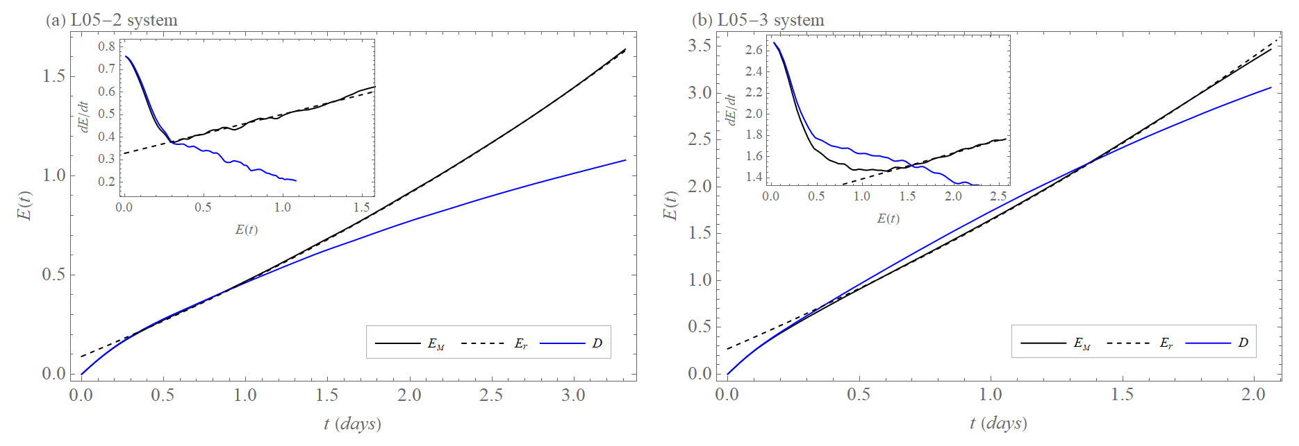
Figure 11 Time evolution of drift D (blue), model error E_M (black), and approximation by exponential growth with model error E_r (dashed black). The inset shows the tendency (rate) of drift $\mathrm{d}D/\mathrm{d}t$ (blue), model error $\mathrm{d}{E}_{\mathrm{r}}/\mathrm{d}t$ (black), and dE_r (dashed black) as a function of D(t), E_M(t), and E_r(t). The difference (a) between the L05-1 system and the L05-2 system and (b) between the L05-1 system and the L05-3 system.

In particular, in the L05-3 model, for the times where the model error growth E_M(t) can be fitted by E_r(t), the drift D(t) first overestimates the model error growth E_M. Following this, a significantly slower growth of the drift D relative to the model error growth E_M is observed, corresponding to a decrease in the growth rate (tendency) of the drift $\mathrm{d}D/\mathrm{d}t\left(D\right)$ compared to the increase in the model error growth rate (tendency) (insets in Fig. 11).

As already mentioned in Sect. 2.4, the drift can be viewed as the sum of the displacements from reality, created at each time step of the model, similar to how an error in the initial conditions will create an initial displacement at the initial time. If we interpret the drift increment $D\left(t_k\right)-D\left(t_{k-\mathrm{1}}\right)$ at each time step $\mathrm{\Delta }t=t_k-t_{k-\mathrm{1}}$, $k=\mathrm{1},\mathrm{\dots },K$ as a new initial error at time t_k, then (similar to Orrell et al., 2001) we can model the model error growth E_M by applying the same time evolution assumption to $D\left(t_k\right)-D\left(t_{k-\mathrm{1}}\right)$ as the initial error growth, i.e., the exponential growth $e^{{\mathit{\lambda }}_{D}t}$ driven by the largest Lyapunov exponent λ_D of the model (L05-1 system). However, this growth should set in only at some time in the future since $\mathit{D}\left(t_k\right)-\mathit{D}\left(t_{k-\mathrm{1}}\right)$ does not point into the locally most unstable direction (see Sects. 2.1 and 3.1 for a description of the initial error growth for the L05-1 system). We approximate this behavior in two different ways and will explore which one gives better results. (Fig. 12). In the first, $D\left(t_k\right)-D\left(t_{k-\mathrm{1}}\right)$ evolves with time t_i in a constant approximation as follows:

$$\begin{array}{}\text{(19)}& F_{\text{con}}(t_k;t_i)=\left\{\begin{array}{ll}\mathrm{1}& t_k\le t_i\le t_{M+k}\\ e^{{\mathit{\lambda }}_D(t_i-t_k)}& t_{M+k+\mathrm{1}}\le t_i\le t_K\end{array}\right.,\end{array}$$

while in a linearly decaying approximation it evolves as follows:

$$\begin{array}{}\text{(20)}& F_{\text{lin}}(t_k;t_i)=\left\{\begin{array}{ll}\mathrm{1}-\mathit{\sigma }(t_i-t_k)& t_k\le t_i\le t_{M+k}\\ (\mathrm{1}-\mathit{\sigma }(t_{M+k}-t_k\left)\right)e^{{\mathit{\lambda }}_D(t_i-t_k)}& \\ & t_{M+k+\mathrm{1}}\le t_i\le t_K\end{array}\right..\end{array}$$

M and σ are parameters that we fix empirically. We propose the hypothesis E_D(t) as a description of the model error growth E_M(t) based on the sum of the individual increments of the drift:

$$\begin{array}{}\text{(21)}& {\displaystyle }\begin{array}{rl}{\displaystyle }{E}_M\left(t_i\right)& {\displaystyle }\approx E_{D,\text{ap}}\left(t_i\right)\\ {\displaystyle }& {\displaystyle }={\sum }_{k=\mathrm{1}}^i\left(D\right(t_k)-D(t_{k-\mathrm{1}}\left)\right)\cdot F_{\text{ap}}(t_k;t_i),\end{array}\end{array}$$

where ap is the symbol for the constant (con) or linear (lin) approximation.

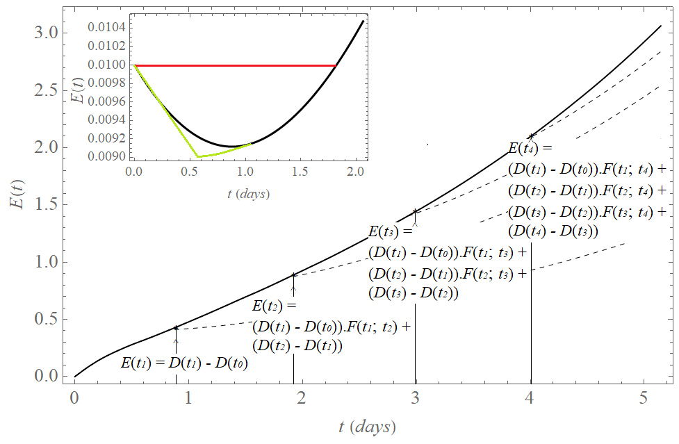
Figure 12 Hypothesis E_D(t) explaining the model error growth E_M(t) (black curve). The drift increment $D\left(t_k\right)-D\left(t_{k-\mathrm{1}}\right)$ at each time step $\mathrm{\Delta }t=t_k-t_{k-\mathrm{1}}$, $k=\mathrm{1},\mathrm{\dots },K$ is taken as the error of the initial conditions with an exponential growth e^λt driven by the largest Lyapunov exponent λ of the model (L05-1 system). Since d(t) does not point into the locally most unstable direction, time evolution of $D\left(t_k\right)-D\left(t_{k-\mathrm{1}}\right)$ decreases in early time (black curve in the inset). A constant (red curve in the inset) or linear decrease (green curve in the inset) approximates this initial decrease. $D\left(t_k\right)-D\left(t_{k-\mathrm{1}}\right)$ evolves with time t_i (dashed curves) in the constant approximation as $F_{\text{con}}(t_k;t_i)=\mathrm{1}$ for $t_k\le t_i\le t_{M+k}$ and $F_{\text{lin}}(t_k;t_i)=e^{\mathit{\lambda }(t_i-t_k)}$ for $t_{M+k+\mathrm{1}}\le t_i\le t_K$, and in the linear approximation as $F_{\text{lin}}(t_k;t_i)=\mathrm{1}-\mathit{\sigma }(t_i-t_k)$ for $t_k\le t_i\le t_{M+k}$ and $F_{\text{lin}}(t_k;t_i)=(\mathrm{1}-\mathit{\sigma }(t_{M+k}-t_k\left)\right)e^{\mathit{\lambda }(t_i-t_k)}$ for $t_{M+k+\mathrm{1}}\le t_i\le t_K$. M and σ are found experimentally. The resulting hypothesis E_D(t) describing the model error growth E_M(t) (black curve) is the sum of the individual increments: $E_M\left(t_i\right)\approx E_{D,\text{ap}}\left(t_i\right)={\sum }_{k=\mathrm{1}}^i\left(D\right(t_k)-D(t_{k-\mathrm{1}}\left)\right)\cdot F_{\text{ap}}(t_k;t_i)$, where ap is the symbol for the constant (con) or linear (lin) approximation.

In comparison to the exponential error growth with model error (with or without saturation), this is a modification in two relevant details. First, the model error is not the same at all time steps into the future like the constant β_r or β_q, but it is the time-into-the-future-dependent increment of the drift D(t). Second, the new contribution in a given time step is not amplified exponentially in the next step, but because it does not point into the locally most unstable direction we let it either remain constant or even decay for a few time steps.

Figure 13 demonstrates how well the model error growth can be approximated by E_D(t), particularly by the approximation with an initial linear decay E_D,lin(t). As the numerical value of the Lyapunov exponent λ_D in the hypothesis E_D(t) we use the one determined as λ_q in the quadratic hypothesis with model error dE_q (Eq. 6), which is λ_q,L05-2=0.27 d⁻¹ from the difference between the L05-1 and L05-2 systems (Fig. 8) and λ_q,L05-3=0.38 d⁻¹ from the difference between the L05-1 and L05-3 systems (Fig. 9). The justification for using the parameter λ_q as λ_D can be found in Bednář et al. (2021). In short, we argue that λ_q is a better estimate of the Lyapunov exponent of the model system than, e.g., λ_r. The parameters M and σ of the hypotheses E_D(t) are determined empirically. It is, however, a bit puzzling that when using the value λ_q in E_D,lin(t), we can approximate that part of the model error growth curve E_M(t), which can also be well approximated by the exponential growth with model error dE_r (Fig. 13), leads to a value of the exponent that is different from λ_q. Therefore, in the next section, we discuss the relationship between the drift D and parameters λ and β in dE_q (Eq. 6) and dE_r (Eq. 5).

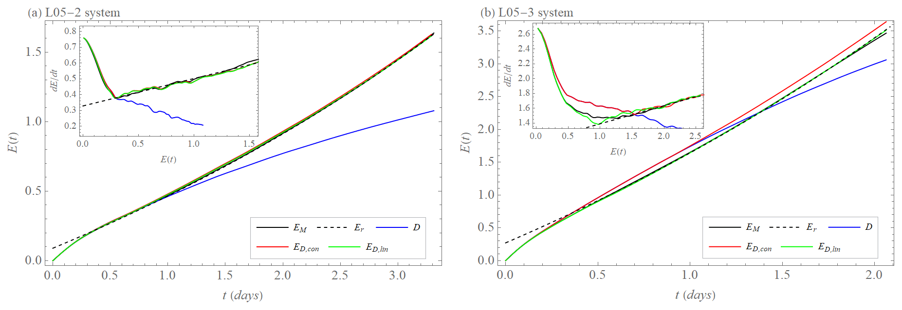
Figure 13 Approximation of model error growth E_M(t) (black curve) by exponential growth with model error E_r (dashed black curve) and by hypotheses E_D,con (Eqs. 19 and 21, red curve) and E_D,lin (Eqs. 20 and 21, green curve) based on drift D (blue curve). (a) Calculation of model error E_M and drift D from the difference between the L05-1 and L05-2 systems. The approximation E_D,con is with M=28 and λ=0.27 d⁻¹, and approximation E_D,lin is with M=24, σ=0.001, and λ=0.27 d⁻¹. (b) Calculation of model error E_M and drift D from the difference between the L05-1 and L05-3 systems. The approximation E_D,con is with M=43 and λ=0.38 d⁻¹, and the approximation E_D,lin is with M=27, σ=0.005, and λ=0.38 d⁻¹. The insets show the time differences (rates) of the quantities as a function of the quantities presented in the main figures.

4.2 Understanding the drift through parameters of the quadratic hypothesis and exponential growth both with model error

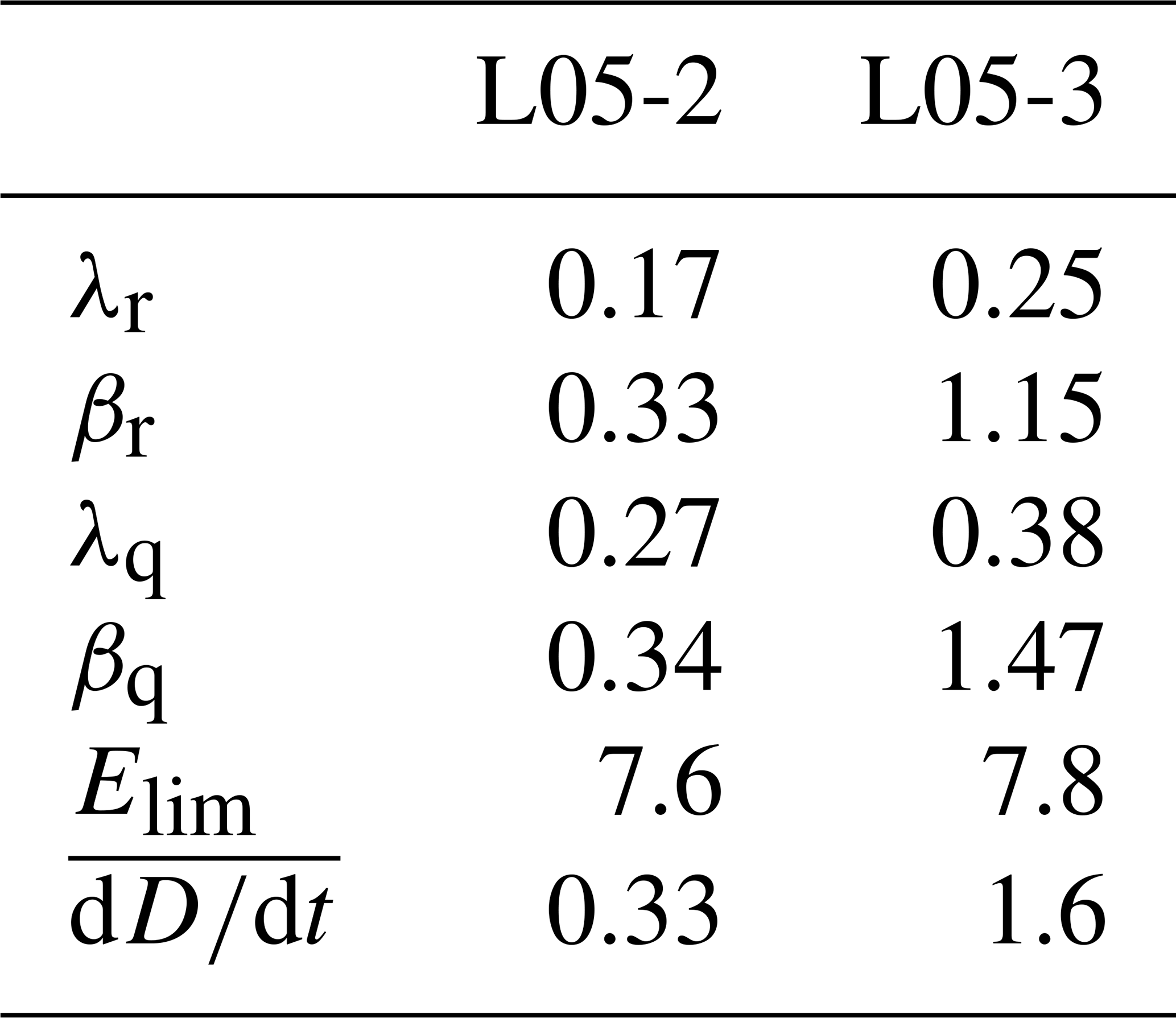
We saw two meaningful approximations to the model error growth curve over lead time: the quadratic hypothesis with model error and the exponential growth with model error. The best-fit parameter values of these two approximations are listed in Table 1. This table shows that $\stackrel{\mathrm{‾}}{\mathrm{d}D/\mathrm{d}t}\approx {\mathit{\beta }}_{\mathrm{q}}$, but the most evident is the difference of the exponential growth exponent λ, where for both realities L05-2 and L05-3 the exponent λ_q of the quadratic hypothesis is larger than λ_r of the best-fit exponential error growth.

Table 1 Table of fitted constants of the different error growth approximations for the L05-2 model and the L05-3 model. All values except E_lim are given as units d⁻¹ or d⁻¹.

To understand the meaning of the parameters of the exponential growth with model error dE_r (Figs. 8 and 9), let us first define the model error growth E_D,0(t) based on the drift D, ignoring the initial decrease caused by D(t) not pointing into the locally most unstable direction:

$$\begin{array}{}\text{(22)}& {\displaystyle }\begin{array}{rl}{\displaystyle }{E}_{D,\mathrm{0}}\left(t_i\right)={\sum }_{k=\mathrm{1}}^i\left(D\right(t_k)-D(t_{k-\mathrm{1}}\left)\right)& {\displaystyle }\cdot e^{{\mathit{\lambda }}_D(t_i-t_k)}\\ {\displaystyle }& {\displaystyle }{t}_k\le t_i\le t_K,\end{array}\end{array}$$

where λ_D is the largest Lyapunov exponent of the model (L05-1 system). The time derivative (calculated from the difference at successive time steps) of E_D,0(t) is

$$\begin{array}{}\text{(23)}& {\displaystyle \frac{\mathrm{d}{E}_{D,\mathrm{0}}}{\mathrm{d}t}}\left(E_{D,\mathrm{0}}\right)={\mathit{\lambda }}_D\cdot E_{D,\mathrm{0}}+{\displaystyle \frac{\mathrm{d}D}{\mathrm{d}t}}\left(E_{D,\mathrm{0}}\right),\end{array}$$

where $\mathrm{d}D/\mathrm{d}t\left(E_{D,\mathrm{0}}\right(t_k\left)\right)=\mathrm{d}D/\mathrm{d}t\left(t_k\right)$, meaning that due to the monotonicity of E_D,0(t) in time, we can exchange the dependence on t by the dependence on E_D,0(t) (see Fig. 14). Equation (23) now claims that the dashed red curve, which is λ_DE, plus the values of the blue curve taken at corresponding times t_k, sum up to yield the red curve E_D(E(t)), where we approximate the slope of the linear increase of the red curve by the slope of the black curve, which describes the observed total error.

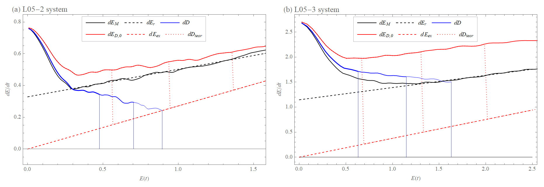
Figure 14 The validity of Eq. (23) ($\mathrm{d}D/\mathrm{d}t\left(D\right(t_k\left)\right)=\mathrm{d}D/\mathrm{d}t\left(E_{D,\mathrm{0}}\right(t_k\left)\right)=\frac{\mathrm{d}{E}_{D,\mathrm{0}}}{\mathrm{d}t}\left(E_{D,\mathrm{0}}\right(t_k\left)\right)-\mathit{\lambda }\cdot E_{D,\mathrm{0}}\left(t_k\right)$) is shown by vertical lines, where the length of the blue lines is the same as the length of the dotted red dD_teor lines at times t₁=1, t₂=1.75, and t₃=2.5 d (from left to right) for (a) the difference between the L05-1 and L05-2 systems and at times t₁=0.3, t₂=0.6, and t₃=0.9 d (from left to right) for (b) difference between L05-1 and L05-3 systems, where $\mathrm{d}D=\mathrm{d}D/\mathrm{d}t\left(D\right)$ (Eq. 18, blue curve) is time difference of drift, $\mathrm{d}{E}_M=\mathrm{d}{E}_M/\mathrm{d}t\left(E_M\right)$ (Eq. 14, black curve) is model error growth, $\mathrm{d}{E}_{D,\mathrm{0}}=\mathrm{d}{E}_{D,\mathrm{0}}/\mathrm{d}t\left(E_{D,\mathrm{0}}\right)$ is a hypothesis Eq. (23) (red curve), dE_r (Eq. 5, dashed black curve) is exponential growth with model error ($\mathrm{d}{E}_{\text{r,L05-2}}=\mathrm{0.17}\cdot E+\mathrm{0.33}$, $\mathrm{d}{E}_{\text{r,L05-3}}=\mathrm{0.25}\cdot E+\mathrm{1.15}$), and dE_ex (Eq. 1, dashed red line) is exponential growth with the value of λ determined from the quadratic hypothesis with model error dE_q (Eq. 6) (${\mathit{\lambda }}_{\text{L05-2}}\to \mathrm{d}{E}_{\mathrm{q}}=(\mathrm{0.27}\cdot E+\mathrm{0.34})(\mathrm{1}-E/\mathrm{7.6})$ and ${\mathit{\lambda }}_{\text{L05-3}}\to \mathrm{d}{E}_{\mathrm{q}}=(\mathrm{0.38}\cdot E+\mathrm{1.47})(\mathrm{1}-E/\mathrm{7.8})$).

We focus now on those parts of the three curves E>0.3 for L02-5 or for E>0.5 for L05-3. As has been said above, we observe that in this range of E, $\mathrm{d}{E}_{D,\mathrm{0}}/\mathrm{d}t\left(E_{D,\mathrm{0}}\right)$ (Fig. 14, red curve) has the same growth rate (tendency) as $\mathrm{d}{E}_M/\mathrm{d}t\left(E_M\right)$ (Fig. 14, black curve), which is expressed by λ_r, fitting the E_r(t) behavior of Eq. (5) to the data (Fig. 14, dashed black curve, λ_r,L05-2=0.17 d⁻¹, λ_r,L05-3=0.25 d⁻¹) If we compare these parameter values to the fit using the quadratic hypothesis with model error, we see that λ_r is smaller than λ_q of dE_q (λ_q,L05-2=0.27 d⁻¹, λ_q,L05-3=0.38 d⁻¹). In our interpretation of the model errors involving the drift, this is due to the decrease in the drift growth rate $\mathrm{d}D/\mathrm{d}t\left(D\right(t_k\left)\right)$ over time (Fig. 14, blue curve). Hence, β_r of the dE_r approximation of $\mathrm{d}{E}_{D,\mathrm{0}}/\mathrm{d}t\left(E_{D,\mathrm{0}}\right)$ is then an extrapolation of the linear decline of $\mathrm{d}D/\mathrm{d}t\left(E_{D,\mathrm{0}}\right(t_k\left)\right)$ to $E_{D,\mathrm{0}}\left(t_{\mathrm{0}}\right)=\mathrm{0}$. Therefore, if we solve Eq. (23) for $\mathrm{d}D/\mathrm{d}t$ and define $\mathrm{d}D/\mathrm{d}t\left(E_{D,\mathrm{0}}\right(t_k\left)\right)\approx {\mathit{\beta }}_D-{\mathit{\alpha }}_D{E}_{D,\mathrm{0}}$, then β_r=β_D. Equation (23) can be used to determine the drift decrease rate α_D: ${\mathit{\lambda }}_{\mathrm{r}}{E}_{D,\mathrm{0}}+{\mathit{\beta }}_{\mathrm{r}}={\mathit{\lambda }}_{\mathrm{q}}{E}_{D,\mathrm{0}}-{\mathit{\alpha }}_D{E}_{D,\mathrm{0}}+{\mathit{\beta }}_D\to {\mathit{\alpha }}_D=({\mathit{\lambda }}_{\mathrm{q}}-{\mathit{\lambda }}_{\mathrm{r}})$. However, β_r=β_D is not the same as β_r in $\mathrm{d}{E}_M/\mathrm{d}t$ (Fig. 14, black curve) because it is reduced by the transition term expressed by Eqs. (20) and (21) and α_D is valid for $\mathrm{d}D/\mathrm{d}t\left(E_{D,\mathrm{0}}\right)$ and not for $\mathrm{d}D/\mathrm{d}t\left(D\right)$. In general, because $\mathrm{d}D/\mathrm{d}t\left(E_{D,\mathrm{0}}\right(t_k\left)\right)\approx {\mathit{\beta }}_D-{\mathit{\alpha }}_D{E}_{D,\mathrm{0}}$ tends to decrease, λ_q>λ_r. Since $\mathrm{d}{E}_M/\mathrm{d}t\left(E_M\right)$ is almost identical to $\mathrm{d}{E}_{M+\text{ie}}/\mathrm{d}t\left(E_M\right)$ and differs only in the early stage of development, the approximations of dE_q and dE_r are only marginally affected (Figs. 8a and 9a). Therefore, information about the drift D can be derived from these hypotheses also for the variant with initial and model error.

For the sole initial condition error, we found that λ_q≤λ_r, but this describes a setting very different from model error. In the initial condition error, we compare the forecast and reality of a given high-resolution model, which indeed has much larger error growth exponents for short times and small errors due to small-scale degrees of freedom. As soon as we talk about model errors (with or without initial error), we use the low-resolution L05-1 model for forecasts, and hence its parameters are relevant for the propagation of errors.

In summary, we propose a new interpretation of the growth of forecast errors due to model errors: model errors in successive time steps of the forecasts are only weakly correlated. Therefore, modeling them by a constant term in the error growth dE is inappropriate. The observed model forecast error growth can be modeled much more accurately if we use the accumulated model errors called drift, interpret the drift increments as additional initial condition errors, and propagate these forward in time. The decrease of the drift growth rate over forecast time can then explain the growth rate of the model errors. Depending on what data are observed, one can either use the drift to predict the forecast errors or use the forecast errors to infer the drift due to model error.

5 Error growth in the ECMWF systems

For the ECMWF forecasting system, we cannot perform error growth experiments, but we can check average forecast errors as a function of lead time. We therefore apply the new way of assessing the model error to the error growth E_EFS(t) of the 500 hPa geopotential height values (Bednář, 2023) calculated (Magnusson and Kallen, 2013) as 25 annual averages over the Northern Hemisphere (20–90°) obtained daily from 1 January 1987 to 31 December 2011. Over this period, we determine the decline in the average initial displacements of the model from reality per unit of time using the parameter β_q of the quadratic hypothesis with model error. Since the parameter β is also used to describe an upscale error growth rate from small-scale processes (Zhang et al., 2019), we check whether λ_q>λ_r, as defined in Sect. 5.2, for β_q determined by model error and λ_q≤λ_r for β_q determined from small-scale processes (see Sect. 4).

5.1 Methods of calculation

To eliminate the effects of model errors, the initial error growth curve E_EFS,ie(t) is calculated as the differences between two operational forecasts issued with 1 d lag for the same day. Specifically, we evaluate these for 27 different lead times and used the following pairs of lead times in hours: 0–24, 6–30, ..., 96–120, with 6 h shift, and from 108–132, 120–144, ..., 216–240 with 12 h shift. Detailed information about calculating the error growth of the ECMWF forecasting system can be found in Lorenz (1982). The error growth rate (tendency) is $\mathrm{d}{E}_{\text{EFS,ie}}/\mathrm{d}t\approx \left(E_{\text{EFS,ie}}\right(t+\mathrm{\Delta }t)-E_{\text{EFS,ie}}(t\left)\right)/\mathrm{\Delta }t$ with Δt=6 h for the first 17 time steps and Δt=12 h for the rest. It is evident that this data analysis solely used data produced by the very same model. One can understand this 1 d offset between two forecasts in the following way. At day 0, we use some initial condition and propagate it forward in time. At day 1, when a new forecast starts with new initial conditions, these can be interpreted as perturbations to the day 1 forecast started at day 0. Therefore, comparing these two forecasts for the very same day as a function of lead time gives us the initial condition error growth. The only disadvantage of this procedure is that we cannot control the magnitude of the perturbation. What we interpret as perturbation is the deviation of the true forecast at day 1 from the new analysis, which is used to initialize the new forecast.

The initial and model error growth curve $E_{\text{EFS},M+\text{ie}}\left(t\right)$ is calculated as differences between operational forecasts and analyses from ERA-Interim for a given day. Forecasts range from 0.5 d ago relative to the given day to 10 d ago, with time step Δt=12 h. The difference between operational analysis and analysis from ERA-Interim is taken as the initial error. The error growth rate (tendency) is $\mathrm{d}{E}_{\text{EFS},M+\text{ie}}/\mathrm{d}t\approx \left(E_{\text{EFS},M+\text{ie}}\right(t+\mathrm{\Delta }t)-E_{\text{EFS},M+\text{ie}}(t\left)\right)/\mathrm{\Delta }t$ with Δt=12 h.

5.2 Results and comparisons

From the data, we calculate 25 annual averages of the initial error growth curve E_EFS,ie(t) and 25 annual averages of the initial and model error growth curve $E_{\text{EFS},M+\text{ie}}\left(t\right)$ and their growth rates (tendencies) $\mathrm{d}{E}_{\text{EFS,ie}}/\mathrm{d}t$ and $\mathrm{d}{E}_{\text{EFS},M+\text{ie}}/\mathrm{d}t$. We approximate the growth rates by the exponential growth with model error dE_r and by the quadratic hypothesis with model error dE_q. Because the data are only up to 10 d and therefore do not cover the entire growth curve and because dE_q is a three-parameter approximation, we first discuss the error in parameter estimation. Magnusson and Kallen (2013) showed that the error saturation parameter E_lim estimated from the dE_q hypothesis underestimates the true limiting value. Bednář et al. (2021) showed that the deviations of the values of λ_q and β_q of dE_q from the true values are anti-correlated, meaning that when one is overestimated, the other is underestimated. The average value of λ_q over 25 annual averages of E_EFS,ie(t) and $E_{\text{EFS},M+\text{ie}}\left(t\right)$ has been determined by Bednář et al. (2021) to be ${\stackrel{\mathrm{‾}}{\mathit{\lambda }}}_{\mathrm{q}}=\mathrm{0.35}$ d⁻¹, and to approximate the data, we fix λ_q to this value. Therefore, we decrease the oscillation of β_q and bring E_lim of dE_q closer to the values determined by Magnusson and Kallen (2013). The fact that E_lim is closer to the theoretical limit values estimated by Magnusson and Kallen (2013) justifies this approach.

The resulting values are shown in Fig. 15. We find that λ_r,ie≥λ_q,ie and ${\mathit{\lambda }}_{\mathrm{r},M+\text{ie}}<{\mathit{\lambda }}_{\mathrm{q},M+\text{ie}}$, which satisfies the hypothesis presented in Sect. 4.2. Here, ${\mathit{\lambda }}_{\mathrm{r},M+\text{ie}}$ (Fig. 15a, solid red curve) has an approximately constant value, showing approximately the same decrease in α_D = the drift rate $\mathrm{d}D/\mathrm{d}t\left(D\right)$ over the years because it is shown in Sect. 4.2 that ${\mathit{\alpha }}_D=({\mathit{\lambda }}_{\mathrm{q},M+\text{ie}}-{\mathit{\lambda }}_{\mathrm{r},M+\text{ie}})$.

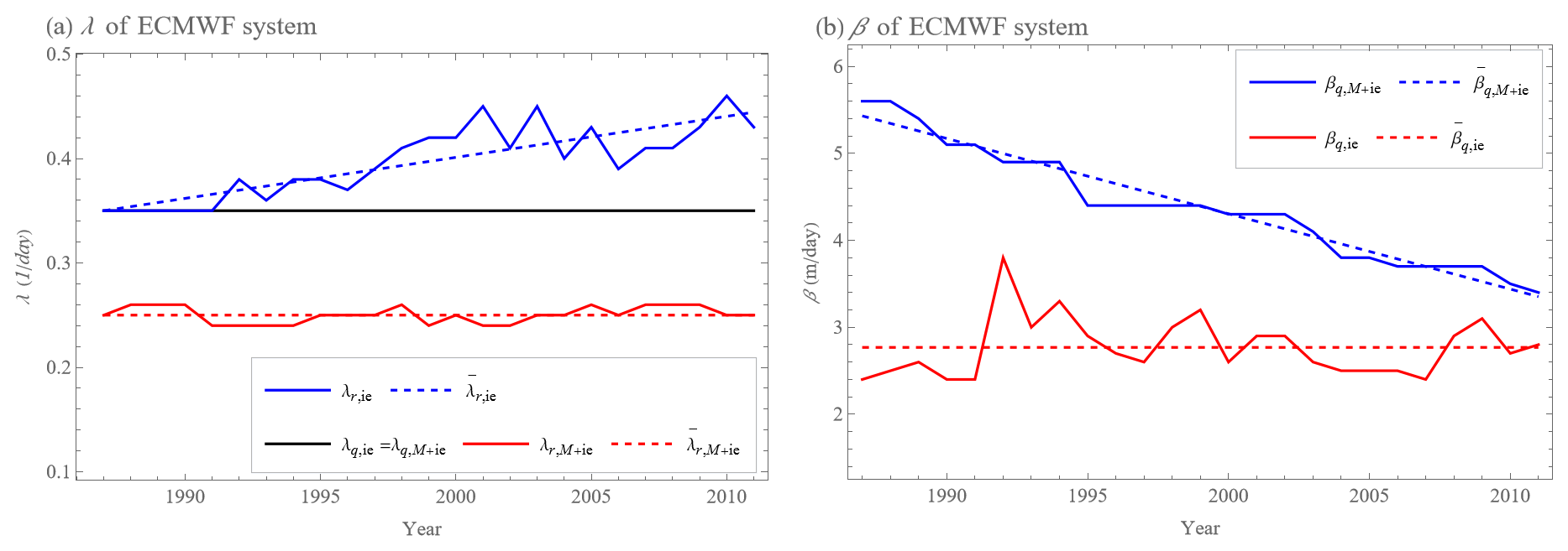
Figure 15 Values of parameters λ (a) and β (b) of exponential growth with model error dE_r and quadratic hypothesis with model error dE_q approximated from annual averages (1987–2011) of the error growth tendencies (rates) $\mathrm{d}{E}_{\text{EFS,ie}}/\mathrm{d}t$ and $\mathrm{d}{E}_{\text{EFS},M+\text{ie}}/\mathrm{d}t$ of the ECMWF forecasting system's 500 hPa geopotential height values over the Northern Hemisphere (for more details, see Sect. 5.1). (a) The black curve is ${\stackrel{\mathrm{‾}}{\mathit{\lambda }}}_{\mathrm{q}}=\mathrm{0.35}$ d⁻¹ determined as the average of the approximated λ_q of dE_q hypothesis over 25 annual averages of E_EFS,ie(t) and $E_{\text{EFS},M+\text{ie}}\left(t\right)$. The solid red curve shows the values λ_r of the dE_r approximation of the 25 annual averages of $\mathrm{d}{E}_{\text{EFS},M+\text{ie}}/\mathrm{d}t$. The dashed red curve shows that the best approximation of ${\mathit{\lambda }}_{\mathrm{r},M+\text{ie}}$ is a constant function with ${\stackrel{\mathrm{‾}}{\mathit{\lambda }}}_{\mathrm{r},M+\text{ie}}=\mathrm{0.25}$ d⁻¹. The solid blue curve shows the values λ_r of the dE_r approximation of the 25 annual averages of $\mathrm{d}{E}_{\text{EFS}}/\mathrm{d}t$. The dashed blue curve shows that the best-fitting approximation of λ_r is a linear function ${\stackrel{\mathrm{‾}}{\mathit{\lambda }}}_{\text{r,ie}}$ that increases with time. (b) Values of β_q of dE_q hypothesis approximating 25 annual averages of $\mathrm{d}{E}_{\text{EFS,ie}}/\mathrm{d}t$ (solid red curve) and $\mathrm{d}{E}_{\text{EFS},M+\text{ie}}/\mathrm{d}t$ (solid blue curve). The dashed red curve shows that the best approximation of β_q,ie is a constant function with ${\stackrel{\mathrm{‾}}{\mathit{\beta }}}_{\text{q,ie}}=\mathrm{2.8}$ m d⁻¹. The dashed blue curve shows that the best-fitting approximation of ${\mathit{\beta }}_{\mathrm{q},M+\text{ie}}$ is a linear function ${\stackrel{\mathrm{‾}}{\mathit{\beta }}}_{\text{r,ie}}$ decreasing with time.

For λ_r,ie (Fig. 15a, solid blue curve), an increase over time is observed, indicating an increase in the resolution of the ECMWF system with smaller spatiotemporal-scale phenomena with a larger error growth rate. The parameter ${\mathit{\beta }}_{\mathrm{q},M+\text{ie}}$ (Fig. 15b, solid blue curve) of the quadratic hypothesis with model error (Eq. 6) shows an approximately linear decrease over the years. These values indicate that the average displacement value per unit of time $\mathit{\beta }\approx \stackrel{\mathrm{‾}}{\mathrm{d}D/\mathrm{d}t}$ decreased by 40 % from 1987 to 2011, from 5.6 to 3.4 m d⁻¹. The parameter β_q,ie (Fig. 15b, solid red curve) for the variant with an initial error shows an approximately constant value. Together with a constant value of λ_q,ie (Fig. 15a, black curve), this means that the shape of the error growth rate (tendency) $\mathrm{d}{E}_{\text{ie}}/\mathrm{d}t\left(E_{\text{ie}}\right)$ changes over the years only by adding a part for smaller E_ie as the model better describes smaller spatiotemporal-scale phenomena, but this does not change the overall approximation of dE_q, as can be seen in Fig. 16. These figures also show the similarity to the error growth rates $\mathrm{d}E/\mathrm{d}t$ of the L05-2 and L05-3 systems (Figs. 6–9) and the relevance of fixing λ_q to approximate the data using dE_q.

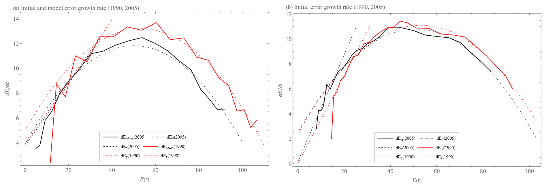
Figure 16 Annual average from 2005 data of the error growth tendencies (rates) $\mathrm{d}{E}_{\text{EFS},M+\text{ie}}/\mathrm{d}t$ (a) and $\mathrm{d}{E}_{\text{EFS,ie}}/\mathrm{d}t$ (b) of the ECMWF forecasting system's 500 hPa geopotential height values over the Northern Hemisphere (solid curves), approximation by the quadratic hypothesis with model error dE_q (Eq. 6) with a constant value of the parameter λ_q=0.35 d⁻¹ (dashed–dotted curves), and approximation by the exponential growth with model error dE_r (Eq. 5, dashed curves). We compare the data from the year 1990 (red) to those of 2005 (black).

6 Conclusion and discussion

Based on the fact that scale-dependent error growth implies an intrinsic predictability limit, we examined whether omitting atmospheric phenomena, which contribute little to the final value, will improve the predictability of the resulting value. In other words, how does the average forecast error growth change in a model where small-scale phenomena are omitted, but the model error is therefore larger compared to a model where all phenomena are present and the average forecast error growth is scale-dependent. For this, we used the L05 systems defined by Lorenz (2005) and Bednář and Kantz (2022) and the ECMWF systems with data from Magnusson and Kallen (2013) stored in Bednář (2023).

We confirmed that for the multi-scale systems L05-2 and L05-3, the initial error growth E_ie(t) can be described well by the power law dE_p Eq. (3) or the extended power law dE_w Eq. (4), respectively, while a simple exponential growth with model error dE_r (Eq. 5) or the quadratic hypothesis with model error dE_q (Eq. 6) are less appropriate. However, the non-zero parameter β in dE_r and dE_q describing the model error also generally relates the multi-scale nature of the system. We showed that in the L05 and ECMWF data (in contrast to the model error scenario) λ_q≤λ_r, meaning that the approximation of $\mathrm{d}{E}_{\text{ie}}/\mathrm{d}t\left(E_{\text{ie}}\right)$ in the early stage grows faster than the approximation of the whole curve due to the presence of only smaller spatiotemporal scales in this part.

For the scenarios of model error growth E_M(t) and both initial and model error growth E_M+ie(t), we showed the appropriateness of the description using exponential growth with model error dE_r and a quadratic hypothesis with model error dE_q (Figs. 8 and 5). For $\mathrm{d}{E}_M/\mathrm{d}t\left(E_M\right)$, we explained the initial decline and subsequent growth described by dE_r using the drift D (Fig. 11) defined by Orrell et al. (2001), which we extended using a hypothesis that views the drift D as a succession of initial errors followed by an exponential time evolution driven by the largest Lyapunov exponent λ of the model after a transition period (Fig. 12). We identified that λ≈λ_q, and the validity of λ_q>λ_r based on the drift evolution was verified in the L05 and ECMWF systems (Fig. 14 and Eq. 21). For the L05 systems, we have demonstrated that ${\mathit{\beta }}_{\mathrm{q}}\approx \stackrel{\mathrm{‾}}{\mathrm{d}D/\mathrm{d}t}$, i.e., that from the β_q value of the quadratic hypothesis with model error dE_q the average displacement per unit time (average drift rate) can be determined.

For ECMWF systems (forecast of 500 hPa geopotential height), this means that from 1987 to 2011 we observe a decrease in the model error by approximately 40 % from an average displacement value of 5.6 to 3.4 m d⁻¹. Note that while in 1987 the error in initial displacement (initial error) was approximately 16 m (Magnusson and Kallen, 2013; Bednář et al., 2021), for the variant with initial and model error, a displacement of 5.6 m is produced every day in addition to this value. In 2011, the initial displacement was 6 m; for the variant with initial and model error, an average displacement of 3.4 m is produced daily. Thus, we observe a significant contribution of the model error to the error growth. This is also why the findings from the model error growth scenario can be applied to the initial and model error growth scenario, where the initial and model error growth goes asymptotically to the model error growth.

It is also why omitting atmospheric phenomena, which contribute little to the final value, will not improve the predictability of the resulting value. The average prediction error grows faster in a model where small-scale phenomena are omitted, but the model error is therefore created, compared to a model where all phenomena are present, but the average forecast error growth is scale-dependent (Fig. 10).

We now discuss the possibility that the growth of the displacement produced by the model error may also be scale-dependent. In our case, the model was an L05-1 system, i.e., a system with one scale and exponential error growth (E_D(t) hypothesis). A variant where the L05-2 system was used as the model and the L05-3 system as the reality was also tested. The resulting model error growth is approximately identical to the previous variant (L05-1 system as the model and L05-3 system as the reality), i.e., adding a small scale did not affect the exponential growth of the drift D increment. However, it should be noted that the magnitude of the average drift per unit of time ${\mathit{\beta }}_{\mathrm{q}}\approx \stackrel{\mathrm{‾}}{\mathrm{d}D/\mathrm{d}t}$ is much greater than the limit (saturation) value of small-scale error magnitude E_2,lim, and thus we are already in the region of exponential error growth of large-scale variables. For the ECMWF system, it can be seen (Fig. 15) that over the years that the values of a parameter β_q of the dE_q approximation of average initial error growth E_ie(t) and initial and model error growth E_ie+M(t) converge, and the growth curves of the two variants are similar for the later analyzed years, as also confirmed by Froude et al. (2013). This means that, in contrast to the presented results of the L05 system, the drift rate of these years is low, and the issue of scale-dependent growth of the drift D increment is relevant and should be further investigated.

Another topic for further research is extending the E_D(t) hypothesis (Eq. 21) to describe the model error growth E_M(t) over the entire range up to saturation rather than just the early part where exponential growth is valid. For the part of the time evolution of the model error where the growth slows down and reaches saturation, it can be seen that the drift must reach its limiting value and then no longer contributes to the model error growth and that the exponential growth of the drift increment must slow down and reach its limiting value. However, the specific form needs to be investigated.

Appendix A: Lorenz's L05 systems

The L05-1 system was introduced by Lorenz (2005) as a spatial continuity modification of the Lorenz (1996) system with N variables connected by governing equations:

$$\begin{array}{}\text{(A1)}& {\displaystyle \frac{\mathrm{d}{X}_n}{\mathrm{d}t}}=[X,X{]}_{L,n}-X_n+F,\end{array}$$

where

$$\begin{array}{ll}{\displaystyle }& {\displaystyle }[X,X{]}_{L,n}=\\ {\displaystyle }& {\displaystyle }\sum _{j=-J}^J{}^{\prime }\sum _{i=-J}^J{}^{\prime }(-X_{n-\mathrm{2}L-i}{X}_{n-L-j}+X_{n-L+j-i}{X}_{n+L+j})/L^{\mathrm{2}},\end{array}$$

$n=\mathrm{1},\mathrm{\dots },N$. X_n are unspecified (i.e., unrelated to actual physical variables) scalar meteorological quantities (units), F is a constant representing external forcing, and t is time. The index is cyclic so that $X_{n-N}=X_{n+N}=X_n$ and variables can be viewed as existing around a latitude circle. If L is even, $\sum {}^{\prime }$ denotes a modified summation in which the first and last terms are to be divided by 2. If L is odd, $\sum {}^{\prime }$ denotes an ordinary summation. Generally, L is much smaller than N and $J=L/\mathrm{2}$ if L is even and $J=(L-\mathrm{1})/\mathrm{2}$ if L is odd. To a certain extent, the model quantitatively describes weather systems, but unlike the well-known Lorenz model of atmospheric convection (Lorenz, 1963), it cannot be derived from any atmospheric dynamic equations. The motivation was to formulate the simplest possible set of dissipative chaotically behaving differential equations that share some properties with the “real” atmosphere. Although mechanisms such as potential vorticity generation are lacking in the equations, the model generates five to seven main highs and lows corresponding to planetary waves (Rossby waves). To keep five to seven main highs and lows, Lorenz (2005) suggested a ratio $N/L=\mathrm{30}$ and F=15. The choice of parameters F and the setting of time unit=5 d is also made to obtain a similar value of the largest Lyapunov exponent to that of the ECMWF forecasting system (Lorenz, 2005).

The L05-2 system (extension to two spatiotemporal scales) was also introduced by Lorenz (2005) as a modification of the two-scale Lorenz (1996) system, where scales were coupled by linear terms that together do not alter the large-scale plus small-scale energy and where small-scale variables were driven entirely by the coupling. Rewriting the equations of the L05-1 system, we would get

$$\begin{array}{}\text{(A2)}& {\displaystyle }\mathrm{d}{X}_{\mathrm{1},n}/\mathrm{d}t=[X_{\mathrm{1}},X_{\mathrm{1}}{]}_{L,n}-X_{\mathrm{1},n}-c{X}_{\mathrm{2},n}+F,\text{(A3)}& {\displaystyle }\mathrm{d}{X}_{\mathrm{2},n}/\mathrm{d}t=b^{\mathrm{2}}[X_{\mathrm{2}},X_{\mathrm{2}}{]}_{\mathrm{1},n}-b{X}_{\mathrm{2},n}+c{X}_{\mathrm{1},n},\end{array}$$

where c sets the rapidness of small scale compared to large scale and b sets the small-scale amplitude size compared to large scale. Equations (A2) and (A3) have an unrealistic property compared to the numerical weather prediction systems. The large-scale and small-scale features are represented by separate sets of variables X₁ and X₂ instead of appearing as superimposed features of a single set X_tot. Lorenz (2005) wanted to keep the system as simple as possible, so instead of, for example, Fourier analysis, a procedure for expressing variables X_tot,n as sums of X_1,n and X_2,n was introduced:

$$\begin{array}{}\text{(A4)}& {\displaystyle }{X}_{\mathrm{1},n}=\sum _{i=-I}^I{}^{\prime }(\mathit{\alpha }-\mathit{\omega }|i\left|\right)X_{\text{tot},n+i},\text{(A5)}& {\displaystyle }{X}_{\mathrm{2},n}=X_{\text{tot},n}-X_{\mathrm{1},n}.\end{array}$$

Parameters α, ω, and I are chosen so that X₁ is a low-pass-filtered version of X_tot, and X₂ represents the difference between the full signal X_tot and the filtered signal. By this procedure, X₂ has a much smaller amplitude than X₁, and also its time evolution should be faster since the temporal derivative is related to the spatial derivative via the difference $(X_{\mathrm{1},n+\mathrm{1}}-X_{\mathrm{1},n-\mathrm{2}})$, which for the low-pass-filtered signal X₁ is typically smaller than for the signal X₂.

More precisely, Lorenz's (2005) idea is that the parameters α and ω are chosen so that X₁ equals X_tot whenever X_tot changes quadratically over the longitudes (variables) n−I through n+I. It is when ${\sum }_{i=-I}^I{}^{\prime }(\mathit{\alpha }-\mathit{\omega }|i\left|\right)=\mathrm{1}$ and ${\sum }_{i=-I}^I{}^{\prime }{i}^{\mathrm{2}}(\mathit{\alpha }-\mathit{\beta }|i\left|\right)=\mathrm{0}$. By solving these equations, we get

$$\begin{array}{}\text{(A6)}& {\displaystyle }\mathit{\alpha }=(\mathrm{3}{I}^{\mathrm{2}}+\mathrm{3})/(\mathrm{2}{I}^{\mathrm{3}}+\mathrm{4}I),\text{(A7)}& {\displaystyle }\mathit{\omega }=(\mathrm{2}{I}^{\mathrm{2}}+\mathrm{1})/(I^{\mathrm{4}}+\mathrm{2}{I}^{\mathrm{2}}).\end{array}$$

The procedures (Eqs. A4 and A5) are functions of the interval length $[-I,I]$.

When creating a system $\mathrm{d}{X}_{\text{tot}}/\mathrm{d}t$ as the sum of $\mathrm{d}{X}_{\mathrm{1}}/\mathrm{d}t$ and $\mathrm{d}{X}_{\mathrm{2}}/\mathrm{d}t$ (sum of Eqs. A2 and A3), the coupling term cX_1,n in Eq. (A3), which enables short waves to develop, is combined with the dissipation term $-X_{\mathrm{1},n}$ in Eq. (A2). Therefore, the coupling term can be canceled entirely, or it can appear in X₁ rather than X₂ when X_tot is analyzed, and there might be nothing to enable the short waves in X₂ to grow. Lorenz (2005) reformulated the coupling process by adding a small fraction of X₁ to X₂ so small waves in X₂ can amplify. It is done by replacing $b^{\mathrm{2}}[X_{\mathrm{2}},X_{\mathrm{2}}{]}_{\mathrm{1},n}+c{X}_{\mathrm{1},n}$ by $[X_{\mathrm{2}},X_{\mathrm{2}}+c^{\prime }{X}_{\mathrm{1}}{]}_{\mathrm{1},n}$ in Eq. (A3), and the L05-2 system would be

$$\begin{array}{}\text{(A8)}& {\displaystyle }\begin{array}{rl}{\displaystyle }\mathrm{d}{X}_{\text{tot},n}/\mathrm{d}t=& {\displaystyle }[X_{\mathrm{1}},X_{\mathrm{1}}{]}_{L,n}+b^{\mathrm{2}}[X_{\mathrm{2}},X_{\mathrm{2}}{]}_{\mathrm{1},n}\\ {\displaystyle }& {\displaystyle }+c[X_{\mathrm{2}},X_{\mathrm{1}}{]}_{\mathrm{1},n}-X_{\mathrm{1},n}-b{X}_{\mathrm{2},n}+F,\end{array}\end{array}$$

where $c=c^{\prime }\cdot b^{\mathrm{2}}$.

Based on the L05-2 system (Eqs. A4–A8), Bednář and Kantz (2022) designed a three-level (scales) system (L05-3):

$$\begin{array}{}\text{(A9)}& {\displaystyle }\begin{array}{rl}{\displaystyle }\mathrm{d}{X}_{\text{tot},n}/\mathrm{d}t=& {\displaystyle }[X_{\mathrm{1}},X_{\mathrm{1}}{]}_{L,n}+b_{\mathrm{1}}^{\mathrm{2}}[X_{\mathrm{2}},X_{\mathrm{2}}{]}_{\mathrm{1},n}\\ {\displaystyle }& {\displaystyle }+b_{\mathrm{2}}^{\mathrm{2}}[X_{\mathrm{3}},X_{\mathrm{3}}{]}_{\mathrm{1},n}+c_{\mathrm{1}}[X_{\mathrm{2}},X_{\mathrm{1}}{]}_{\mathrm{1},n}\\ {\displaystyle }& {\displaystyle }+c_{\mathrm{2}}[X_{\mathrm{3}},X_{\mathrm{2}}{]}_{\mathrm{1},n}-X_{\mathrm{1},n}-b_{\mathrm{1}}{X}_{\mathrm{2},n}\\ {\displaystyle }& {\displaystyle }-b_{\mathrm{2}}{X}_{\mathrm{3},n}+F,\end{array}\end{array}$$

where c₁, c₂, b₁, and b₂ are parameters, and the procedures for expressing the variables are

$$\begin{array}{}\text{(A10)}& {\displaystyle }& {\displaystyle }\begin{array}{rl}{\displaystyle }{X}_{\mathrm{1},n}={\sum }_{i=-I_{\mathrm{1}}}^{I_{\mathrm{1}}}{}^{\prime }& {\displaystyle }\left(\right((\mathrm{3}{I}_{\mathrm{1}}^{\mathrm{2}}+\mathrm{3})/(\mathrm{2}{I}_{\mathrm{1}}^{\mathrm{3}}+\mathrm{4}{I}_{\mathrm{1}}))\\ {\displaystyle }& {\displaystyle }-\left(\right(\mathrm{2}{I}_{\mathrm{1}}^{\mathrm{2}}+\mathrm{1})/(I_{\mathrm{1}}^{\mathrm{4}}+\mathrm{2}{I}_{\mathrm{1}}^{\mathrm{2}}\left)\right)\left|i\right|)X_{\text{tot},n+i},\end{array}\text{(A11)}& {\displaystyle }& {\displaystyle }\begin{array}{rl}{\displaystyle }{X}_{\mathrm{2},n}={\sum }_{j=-I_{\mathrm{2}}}^{I_{\mathrm{2}}}{}^{\prime }& {\displaystyle }\left(\right((\mathrm{3}{I}_{\mathrm{2}}^{\mathrm{2}}+\mathrm{3})/(\mathrm{2}{I}_{\mathrm{2}}^{\mathrm{3}}+\mathrm{4}{I}_{\mathrm{2}}))\\ {\displaystyle }& {\displaystyle }-\left(\right(\mathrm{2}{I}_{\mathrm{2}}^{\mathrm{2}}+\mathrm{1})/(I_{\mathrm{2}}^{\mathrm{4}}+\mathrm{2}{I}_{\mathrm{2}}^{\mathrm{2}}\left)\right)\left|j\right|)\\ {\displaystyle }& {\displaystyle }\times (X_{\text{tot},n+j}-X_{\mathrm{1},n+j}),\end{array}\text{(A12)}& {\displaystyle }& {\displaystyle }{X}_{\mathrm{3},n}=X_{\text{tot},n}-X_{\mathrm{2},n}-X_{\mathrm{1},n},\end{array}$$

where I₁ and I₂ set the length of the intervals $[-I,I]$.

The parameters of L05 systems (L05-1, L05-2, L05-3) should be set so that all scales behave chaotically (the largest Lyapunov exponent of each scale is positive) and that all scales have a significant difference in amplitudes and fluctuation rates. For the L05-1 system (Eq. A1), the chaotic behavior is determined by the value of F and the number of variables N. For Eqs. (A2) and (A3), where the forcing F acts only on a large scale, the chaotic behavior of the small scale is created by coupling. The coupling size is cascaded from a large scale to a small one. Because the values of large-scale variables are determined by the forcing F, the F value indirectly affects the small-scale chaotic behavior and must be chosen large enough to ensure chaotic behavior through coupling for all scales (levels). This fact must also apply to L05-2 and L05-3 systems, but procedures (A4) and (A5) for the L05-2 system and (A10)–(A12) for the L05-3 system also affect the scales' chaotic behavior, amplitude, and fluctuation rate through the choice of I (Lorenz, 2005).

To maintain the required properties F=15, N=360, L=12, and J=6 is chosen for the L05-1 system (Fig. 1a). To have the small scale 100 times smaller than the large scale, F=15, N=360, L=12, J=6, b=10, c=1, and I=10 are selected for the L05-2 system (Fig. 2a). For the L05-3 system, with requirements for the medium-scale amplitude to be about 10 times smaller than the large-scale amplitude, the small-scale amplitude to be about 10 times smaller than the medium-scale amplitude, and for the scales to have different oscillation rates (Fig. 3a), F=15, N=360, L=12, J=6, b₁=1, b₂=10, c₁=1, c₂=1, I₁=20, and I₂=10. The calculation is done using a fourth-order Runge–Kutta method with a time step $\mathrm{\Delta }t=\mathrm{1}/\mathrm{240}$ or 0.5 h.