Deep-learning-driven simulations of boundary layer clouds over the Southern Great Plains

Based on long-term observations at the Southern Great Plains site by the Atmospheric Radiation Measurement (ARM) program for training and validation, a deep-learning model is developed to simulate the daytime evolution of boundary layer clouds (BLCs) from the perspective of land–atmosphere coupling. The model takes ARM measurements (including early-morning soundings and diurnally varying surface meteorological conditions and heat fluxes) as inputs and predicts hourly estimates (including cloud occurrence, the positions of cloud boundaries, and the vertical profile of the cloud fraction) as outputs. The deep-learning model offers good agreement with the observed cloud fields, especially in the accuracy with which cloud occurrence and base height are reproduced. When the inputs are substituted by reanalysis data from ERA5 and MERRA-2, the outputs of the deep-learning model provide a better agreement with observation than the cloud fields extracted from ERA5 and MERRA-2 themselves. Thus, the deep-learning model shows great potential to serve as a diagnostic tool for the performance of physics-based models in simulating stratiform and cumulus clouds. By quantifying biases in clouds and attributing them to the simulated atmospheric state variables versus the model-parameterized cloud processes, this observation-based deep-learning model may offer insights into the directions needed to improve the simulation of BLCs in physics-based models for weather forecasting and climate prediction.

1 Introduction

Boundary layer clouds (BLCs), which primarily comprise stratiform and shallow cumuli, exert a profound influence on the Earth's radiative balance (Betts, 2009; Teixeira and Hogan, 2002; Lu et al., 2013; Golaz et al., 2002). Their formation and evolution are critically shaped by the interactions between the surface, the planetary boundary layer (PBL), and the free troposphere (Miao et al., 2019; Berg and Kassianov, 2008; Zhang and Klein, 2013; Guo et al., 2017, 2019; Y. Zhang et al., 2017). Numerous studies have investigated the controlling factors for BLCs, highlighting the pivotal role of the land surface in modulating cloud formation and affecting the spatial and temporal distribution of low clouds (Zhang and Klein, 2010, 2013; Rieck et al., 2014; Xiao et al., 2018; Lareau et al., 2018; Lee et al., 2019; Tang et al., 2019; Tao et al., 2019; Tian et al., 2022).

These clouds, which frequently form in the PBL's entrainment zone, are very challenging to simulate in weather prediction and climate modeling due to the small scales of the physics involved and the complex feedback mechanisms between land surface fluxes, PBL turbulent processes, and cloud microphysics (Miao et al., 2019; Lu et al., 2011; Fast et al., 2019; Morrison et al., 2020; Yang et al., 2018; Nogherotto et al., 2016; Caldwell et al., 2021; Wang et al., 2023; Guo et al., 2019). These challenges are compounded when attempting to represent such processes in global and regional climate models, where the fine-scale interactions are often parameterized in a coarse-resolution grid due to computational constraints (Bretherton et al., 2007; Zheng et al., 2021; Moeng et al., 1996; Randall et al., 2003; Prein et al., 2015). In addition, different cloud regimes exhibit complex nonlinear cloud–land interactions, which pose challenges for observational studies and modeling efforts, particularly for physical parameterizations (Tang et al., 2018; Qian et al., 2024; Sakaguchi et al., 2022; Poll et al., 2022; Tao et al., 2021).

As an emerging tool, machine learning (ML) has been widely employed for a variety of environmental and atmospheric studies (e.g., McGovern et al., 2017; Gagne et al., 2019; Vassallo et al., 2020; Cadeddu et al., 2009; Molero et al., 2022; Guo et al., 2024). Specifically, ML techniques are increasingly being employed to simulate and estimate convection and precipitation, which are crucial for accurate weather forecasting and climate modeling (Mooers et al., 2021; Wang et al., 2020; O'Gorman and Dwyer, 2018; Gentine et al., 2018; Zhang et al., 2021). For example, Rasp (2020) presents algorithms for the implementation of coupled learning in cloud-resolving models and the super-parameterization framework. Similarly, ML tools have been applied to leverage observational data for the refinement of convection parameterizations, offering more insights into convective triggering (Zhang et al., 2021). In addition, ML has been used to emulate convection schemes and develop parameterizations using data from advanced simulations (O'Gorman and Dwyer, 2018; Gentine et al., 2018). Furthermore, Haynes et al. (2022) developed pixel-based ML-based methods of detecting low clouds, with a focus on improving detection in multilayer cloud situations and with specific attention given to improving cloud characteristics. Despite the considerable advancements brought by ML, there are persistent challenges in accurately simulating the vertical structure of clouds as well as their complex relationships with the land surface.

The Southern Great Plains (SGP) site, which is part of the US Department of Energy Atmospheric Radiation Measurement (ARM) program, is crucial for cloud evaluation and climatology studies in modeling efforts. Recognized globally as a leading climate research facility, the ARM SGP site (located 36.607° N, 97.488° W) has been collecting a wealth of meteorological and radiative measurements and can offer data that spans over 2 decades (Sisterson et al., 2016). The rich dataset from the ARM SGP site can help address persistent challenges in cloud modeling. This study leverages these extensive observations to build a deep-learning model that serves as an observation-based “emulator” for simulating BLCs. Our model enhances the estimations for cloud fields of BLCs, particularly those for cloud occurrence, position, and fraction. Furthermore, a critical assessment of our model in comparison with existing reanalysis datasets, including MERRA-2 and ERA5, highlights the improvement in estimating cloud vertical structure. Our study analyzes the model's performance across different cloud regimes, such as stratiform and cumulus. By undertaking this endeavor, we aim to help bridge the existing gaps between field observations and modeling by providing a deep-learning model of BLCs, thereby improving diagnostics of model performance and enriching our understanding of BLC processes.

2 Data description

2.1 Observations for the development of the deep-learning model

This study utilized the ARM SGP observations during 1998–2020 to serve as training, validation, and testing data for the development of the deep-learning model. Note that all the observations are collected at the central facility in the SGP, a fixed location, which is different from other ML studies that use global data from reanalysis or climate model simulations (e.g., O'Gorman and Dwyer, 2018; Shamekh et al., 2023).

The input data used to train and validate the deep-learning model include early-morning sounding data and diurnally varying surface meteorological conditions and surface turbulent heat fluxes. We take radiosonde (SONDE) measurements at around 06:00 local time to obtain thermodynamic and wind profiles in the PBL and the free atmosphere for use as initial conditions (Holdridge et al., 2011). SONDE launches typically took place 4 times per day at the SGP site, usually at 00:00, 06:00, 12:00, and 18:00 local time. Local time, defined as daylight saving time, is used consistently throughout the year. Each morning profile comprises 46 levels spanning from 0–8 km, including levels at intervals of 50 m from 0 to 1 km, 0.1 km from 1 to 2 km, 0.25 km from 2 to 4 km, and 0.5 km from 4.5 to 8 km. Meanwhile, the collocated surface meteorology systems (MET; Ritsche, 2011) provide a variety of meteorological measurements (i.e., temperature, relative humidity, wind, and pressure) at the surface. Surface sensible- and latent-heat fluxes are taken from the ARM value-added product called the best-estimate fluxes from the bulk aerodynamic calculations of the energy balance Bowen ratio measurements (BAEBBR, Cook, 2018).

In addition, we also use derived variables based on observations as the input fields for the deep-learning model. The lifting condensation level (LCL) is derived from the surface meteorology (Romps, 2017), while the BLH_parcel (the boundary layer height derived from parcel methods) is calculated from the morning temperature profiles and the surface air temperature (Holzworth, 1964; Su and Zhang, 2024; Chu et al., 2019). Specifically, BLH_parcel is defined as the height where the morning potential-temperature profile first exceeds the current surface potential temperature by more than 1.5 K. Meanwhile, BLH_SH (the boundary layer height derived from the sensible heat flux) is calculated from the morning temperature profiles and surface sensible heat (Stull, 1988; Su et al., 2023).

Our study employs hourly cloud fraction data available from the ARM Best Estimate (ARMBE; Xie et al., 2010) dataset as the target data for model outputs when training and validating the deep-learning model. This cloud fraction is developed based on Active Remote Sensing of Clouds (ARSCL; Clothiaux et al., 2000, 2001; Kollias et al., 2020), which utilizes the best estimates from a ceilometer for the lowest cloud bases and integrates micro-pulse lidar, ceilometer, and cloud radar data to define cloud tops and the cloud fraction. In addition, to construct learning targets, the base of the BLC is determined as the lowest altitude where the cloud fraction first exceeds 1 %, and the cloud top is identified as the point where the cloud fraction transitions from exceeding 1 % to falling below this threshold. In multi-layer systems, the deep neural network (DNN) model is trained based on the lowest cloud layer when it is coupled with the land surface. However, we do not exclude multiple-layer cloudy cases if their vertical fractions are continuous from the lower to the upper layer.

Based on ARM observations, this study develops an advanced deep-learning framework to simulate the BLCs using detailed observational data, including SONDE profiles, surface meteorological measurements, and ARSCL, from the SGP site. This framework is designed for BLCs and places particular emphasis on cloud–land coupling mechanisms. By integrating morning SONDE observations with diurnally varying surface fluxes and meteorological data, this deep-learning model is capable of diagnosing the initiation and evolution of low clouds, especially those coupled with land surface processes.

2.2 Classification of coupled boundary layer clouds from observations

The deep-learning model in this study aims to simulate BLCs that are strongly coupled with boundary layer and land surface processes. The classification of clouds described below is used to filter the BLCs based on the concept of cloud–land coupling and is important for the training and analysis of the deep-learning model. Here, we treat BLCs as synonymous with land-coupled clouds, in contrast to clouds that are decoupled from the PBL and land surface.

Coupled clouds are identified when the cloud base height (CBH), as derived from the ceilometer, aligns with or is below the lidar-detected PBL top height to within 0.2 km and the calculated surface-based LCL (Romps, 2017) falls within the maximum allowable range of 0.7 km (Su et al., 2022). PBL height data (Su et al., 2020; Roldán-Henao et al., 2024) are available through the ARM database. This alignment is indicative of clouds that are directly influenced by surface-driven processes. Meanwhile, a cloud thickness threshold (<4 km) is applied to ensure the occurrence of BLCs (i.e., not deep convective clouds).

Within the scope of land-coupled clouds, we further classify the observed daytime BLCs into cumulus and stratiform categories following the methodology in Su et al. (2024). Stratiform cloud days are identified as those with prolonged (lasting more than 3 h) overcast conditions during the daytime and a maximum cloud fraction exceeding 90 % based on ARSCL data. For cumulus cloud days, two criteria are applied: (1) cloud formations emerge after sunrise, ensuring that they are driven by local convective processes, and (2) there is an absence of stratiform clouds. Based on these criteria, we identify 940 d that are categorized as having a cumulus regime, with 21 % occurring in spring, 56 % in summer, 17 % in fall, and 6 % in winter. Similarly, we identify 657 d that fall within the stratiform cloud regime, with a seasonal distribution of 37 % in spring, 12 % in summer, 23 % in fall, and 28 % in winter. Note that this cloud regime classification is done on a daily basis. To maintain clarity in our analysis, we exclude days with mixed cloud regimes, focusing only on days that exhibit only stratiform or cumulus clouds during the daytime.

2.3 Reanalysis data for the application of the deep-learning model

To demonstrate how to use the deep-learning model, we take advantage of reanalysis datasets from the European Centre for Medium-Range Weather Forecasts' fifth-generation global reanalysis (ERA5; Hersbach et al., 2020) and NASA's Modern-Era Retrospective analysis for Research and Applications Version 2 (MERRA-2; Gelaro et al., 2017). Note that, unlike the aforementioned observational data, reanalysis data are not used for training the deep-learning model; instead, they are used to help illustrate how the deep-learning model may disentangle the potential causes leading to biased cloud simulations.

ERA5 provides hourly atmospheric states and cloud fractions around the SGP by utilizing the Integrated Forecasting System (IFS) and a data assimilation system with a horizontal resolution of 0.25° × 0.25° and a vertical resolution of 25 hPa in the lower atmosphere (700–1000 hPa). The IFS employs a prognostic cloud scheme capable of capturing the evolution of cloud dynamics over consecutive time steps (Tiedtke, 1993), a feature that enhances its utility in time-dependent climate studies.

MERRA-2 provides hourly low-cloud fraction and 3-hourly vertical cloud-fraction profiles at a spatial resolution of 0.67° (longitude) × 0.5° (latitude). MERRA-2 is based on the Goddard Earth Observing System Data Assimilation System Version 5 and utilizes a diagnostic cloud scheme that focuses on the immediate state of clouds (Randles et al., 2017), which is widely used in multiple studies (e.g., Yeo et al., 2022; Kuma et al., 2020; Miao et al., 2019).

Here we acknowledge the local heterogeneity of cloud fields in the area covered by an ERA5 or MERRA-2 grid cell. This inherent discrepancy between the reanalysis data and the ARM SGP observations may arise from the difference between point-based measurements and area-based assimilated grid averages. However, observations at the SGP site, representative of plain regions, have been widely used for evaluating models across scales from climatological and statistical perspectives (e.g., Song et al., 2014; Zheng et al., 2023; L. Zhang et al., 2017).

3 Construction of the deep-learning model for boundary layer clouds

3.1 Structural design of the deep-learning model

This study develops an integrated deep-learning model to simulate BLC over the SGP site. The model design is illustrated in Fig. 1. Traditionally, simulating BLCs involves solving complex equations related to PBL turbulence and cloud microphysical processes. Our approach, however, leverages deep learning to bypass these intricate simulations. By using module-specific hidden layers, the deep-learning model serves as an observation-based “emulator” that directly estimates BLCs from early-morning soundings and surface-related parameters.

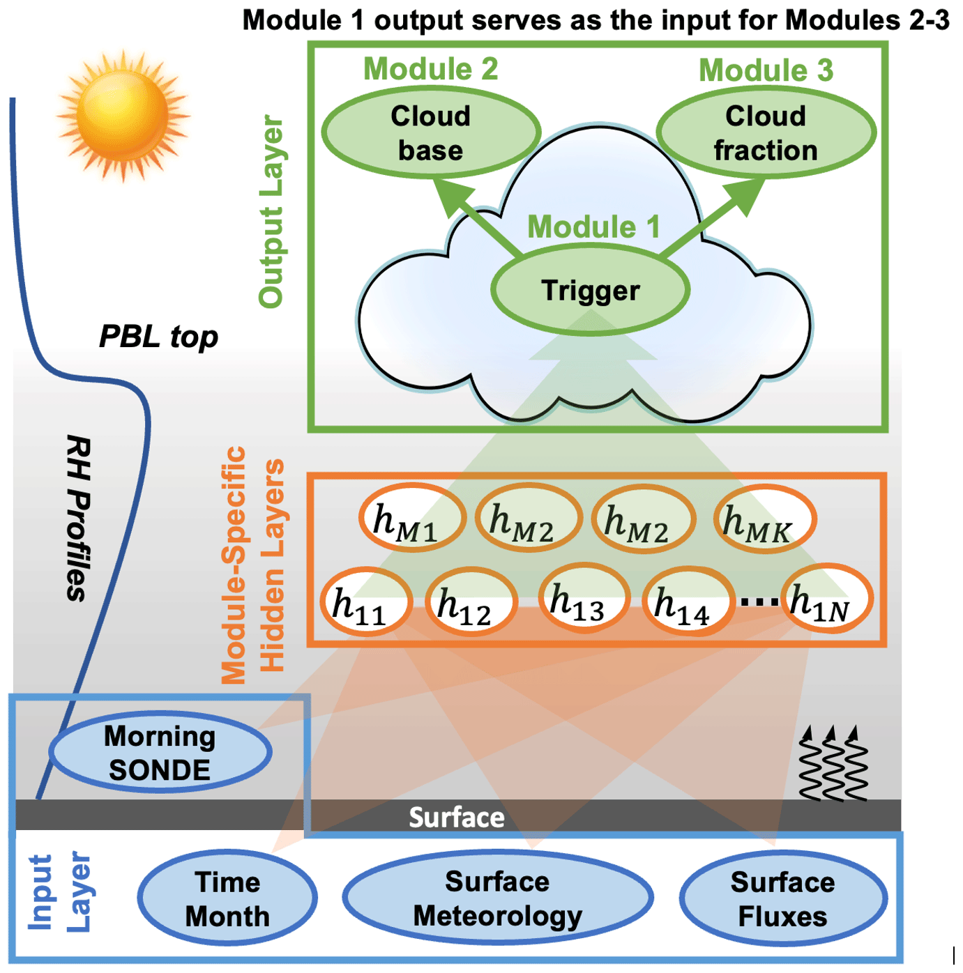
Figure 1 Conceptual diagram of the deep-learning framework for simulating boundary layer cloud (BLC) characteristics over the US Southern Great Plains. Inputs for the deep neural networks (DNNs) include morning meteorological profiles from radiosondes (SONDE), time indicators (i.e., the local time and month), and surface conditions such as fluxes (curved black arrows) and meteorological data. The relevance of relative-humidity (RH) profiles and the planetary boundary layer (PBL) top is emphasized due to their critical role in BLC development. These variables are processed through multiple layers of hidden neurons (h₁₁ to h_MK). Both input and output parameters are provided hourly, except for the morning SONDE data. Separate DNN modules are constructed for each task: Module 1 handles the initiation (trigger) of BLC, Module 2 estimates the cloud base, and Module 3 estimates the cloud fraction and thickness. Together, these models synergize to predict the presence, altitude, and stratification of BLC.

The model is purpose-built to consist of three distinct deep-learning modules, each responsible for a critical aspect of the cloud simulation: (1) the determination of BLC occurrence, (2) the height position of the cloud base, and (3) the cloud thickness and the normalized 10-layered shape of the cloud fraction within cloud boundaries, which jointly yield the hourly averaged vertical structures of BLCs. This modular approach ensures that the estimations are specific for each aspect of the BLCs. Combining cloud thickness and cloud fraction in one module is logical because the vertical distribution of cloud fraction is related to the overall cloud thickness; e.g., thicker clouds are usually associated with larger cloud fractions. Naturally, the cloud top is considered as the cloud base plus the thickness. This separation of tasks enhances the overall reliability and clarity of the model in capturing the various characteristics of BLCs. Note that each of the three deep-learning modules is built upon a DNN with multiple hidden layers.

In the first step, the occurrence module evaluates the likelihood of cloud formation by producing a number between 0 and 1 which we call the “trigger” in the following; a value above 0.5 indicates the presence of clouds. The target value for this module is binary (0 or 1), and the model output is a continuous value between 0 and 1. This occurrence information then feeds into the other two modules – one for locating cloud boundaries and the other for delineating the vertical shape of the cloud fraction in cloudy layers – in parallel. While the cloud-base (or boundary) module and the fraction-thickness (or fraction) module are independent of each other, they collaborate to depict the vertical cloud-fraction profile.

To represent the vertical structure of BLC in the fraction-thickness module, we segment the cloud layer from the base to the top into 10 levels, with each level's thickness varying according to the overall cloud thickness. These values are then interpolated to create a continuous vertical profile of cloud fraction within the BLC boundaries, offering a detailed depiction of the cloud's vertical extent. The vertical position of the layer changes based on the predicted cloud base and top to accurately represent the vertical structure of BLCs. This dynamic approach allows the fraction module to adjust and focus on the relevant portions of the cloud fraction within cloudy layers. Compared to a static height-level approach, which requires the prediction of cloud fraction across a fixed vertical extent (e.g., multiple levels between 0–6 km), our method focuses on the shape of the fraction profile. This ensures that the model is not constrained by fixed vertical levels, allowing for more efficient and robust estimations.

3.2 DNN architecture and configuration

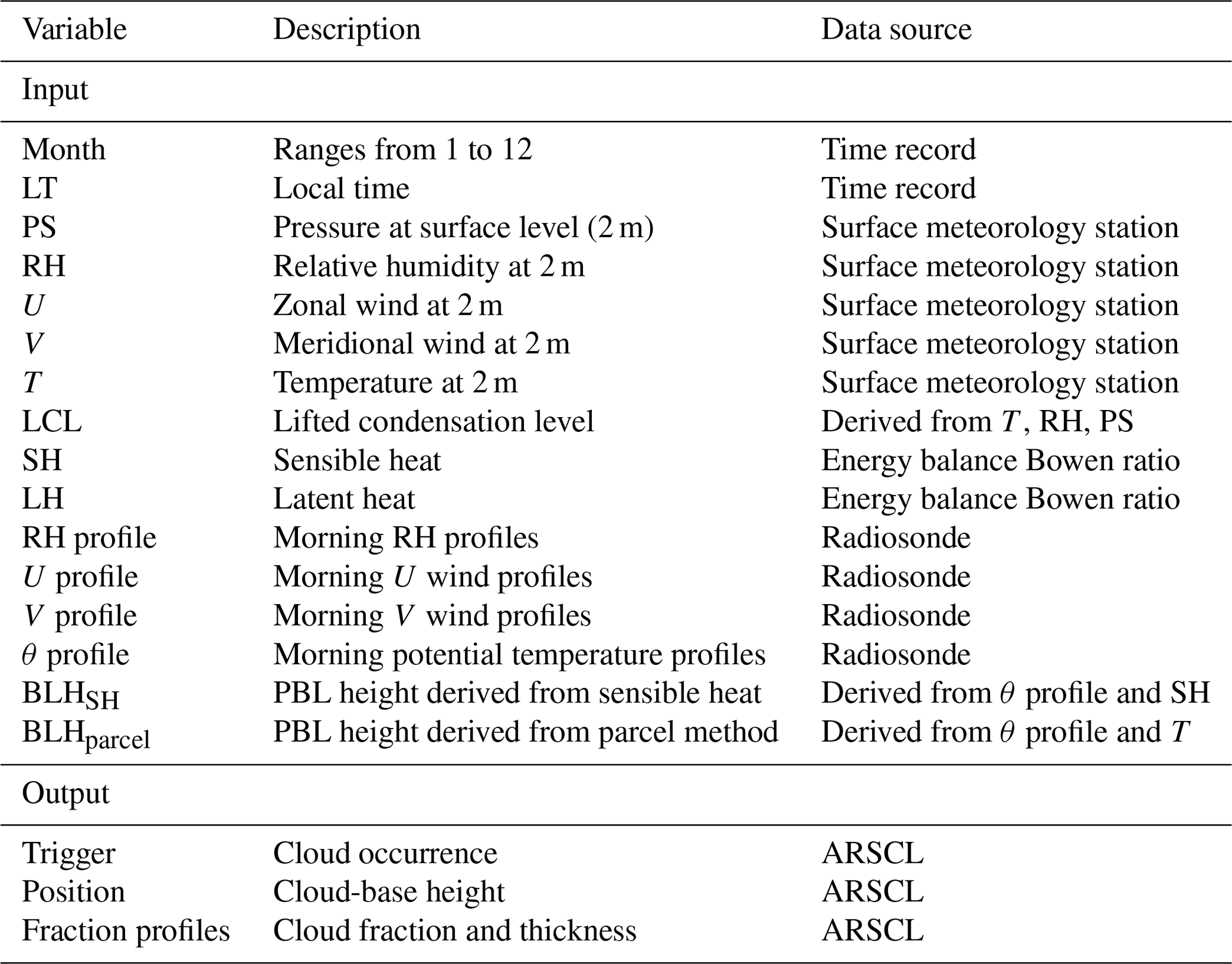
The construction of the deep-learning model uses the TensorFlow Package, developed by Google (https://www.tensorflow.org/, last access: 2 June 2024). Each module in the deep-learning model is constructed based on a separate DNN. The DNN architecture is designed beginning with an input layer reflective of the selected feature set, which includes morning sounding profiles, surface meteorology and heat flux data, and the derived variables such as LCL, BLH_parcel, and BLH_SH. The input surface conditions for predicting the current-hour BLC include data from both the current hour and the previous hour. The input variables for training and validating the deep-learning model are detailed in Table 1, including variable names, descriptions, and data sources, together with the ARMBE cloud fraction profiles used as the learning target for model outputs. Normalization, a preprocessing technique, is applied to both input and target data to scale them to a zero mean and a standard deviation of 1 (Klambauer et al., 2017; Salimans and Kingma, 2016; Raju et al., 2020). This standardization ensures that the data is scaled to a common range and offers some benefits, such as improving the stability and efficiency of the training process.

Table 1 Detailed descriptions of the input and output variables used in the deep-learning models for predicting BLCs. The table includes the variable names, descriptions, and data sources. For the input parameters, the surface meteorology and fluxes are taken from the current and previous hour, while the morning profiles comprise 46 values spanning from 0–8 km at 06:00 LT. Note that the output data are derived from ARSCL (Active Remote Sensing of Clouds). The three outputs correspond to the trigger module, cloud-base module, and fraction-thickness module, respectively.

The architecture of the DNN models is structured and tailored for each module: occurrence, cloud-base, and fraction (or fraction-thickness) estimation. Each module's structure is defined by the number of neurons in its hidden layers. For the occurrence module, the structure consists of four hidden layers with 108, 64, 36, and 24 neurons, respectively. The CBH prediction module is similarly structured with four hidden layers, but it consists of 96, 56, 32, and 24 neurons, respectively. The module for predicting cloud fraction and thickness has a slightly simpler structure, with three hidden layers containing 56, 32, and 24 neurons, respectively.

For the specific configuration, we utilize the ReLU (rectified linear unit) activation function to introduce nonlinearity into the DNN. L2 regularization with a strength of 0.01 is applied to mitigate overfitting by penalizing large weights and encouraging simpler models. Batch normalization is implemented at each layer to normalize the inputs, ensuring a consistent data distribution and stabilizing the learning process. A dropout rate of 0.2 is used to randomly omit neuron connections during training, preventing overfitting and encouraging the network to learn more robust features. The training process is refined with early stopping (further epochs are ceased when the validation loss ceases to improve) and learning-rate reduction (the learning rate is systematically decreased upon encountering plateaus in performance improvement). These callbacks are instrumental in honing the model's performance by ensuring convergence to the accurate estimation of the BLC. Neuron biases are included in the network's architecture and systematically inserted in the hidden layers (Battaglia et al., 2018). The model is compiled using the Adam optimizer with an initial learning rate of 0.01. The loss functions used are mean squared error for regression tasks and binary cross-entropy for binary classification tasks. The batch size during training is set to 32. Early stopping with a patience of 37 epochs is implemented to prevent overfitting and to restore the best weights when the validation loss ceases to improve.

3.3 Model training process and examples

The construction of the deep-learning model commences with the segregation of the ARM observations during 1998–2016 into a training subset (70 %) and a validation subset (30 %). In addition, we save data from 2017–2020 for testing, specifically focusing on this independent period to assess the model's performance. Upon training completion, the model is then evaluated, with its performance metrics examined for accuracy and reliability. This methodical and data-driven process balances complexity with precision, culminating in a robust model capable of simulating BLC features.

The modules within the deep-learning model operate synergistically, with the predicted occurrence of clouds extending into the modules for cloud base and vertical structure (i.e., cloud thickness and shape of the cloud fraction profile). As an example of the model output, Fig. 2 offers a comparative display of diurnal cloud fraction profiles over the SGP, contrasting the observed data with the simulated clouds from the deep-learning model. The model accurately simulates the cloud occurrence and the CBH for these cases: they align well with observations. However, it falls short in simulating the cloud top heights, with especially significant overestimates for stratiform clouds. It also underestimates the maximum cloud fractions for stratiform clouds. The observed maximum cloud fraction for stratiform clouds is close to 1, indicating complete coverage; however, this aspect is not fully replicated by the deep-learning model. The third case also falls into the category of stratiform clouds and is characterized by an observed cloud fraction exceeding 0.9. However, the presence of multiple local maxima within the cloud fraction profile indicates a relatively complex structure. This complexity poses a challenge to the model, as the DNN is not fully capable of capturing the internal variations within the convective system. Instead, the model tends to produce a more uniform cloud fraction across this convective system. Despite these variances, the model-derived cloud bases and occurrence demonstrate high consistency with observations, highlighting its value in the cloud simulations.

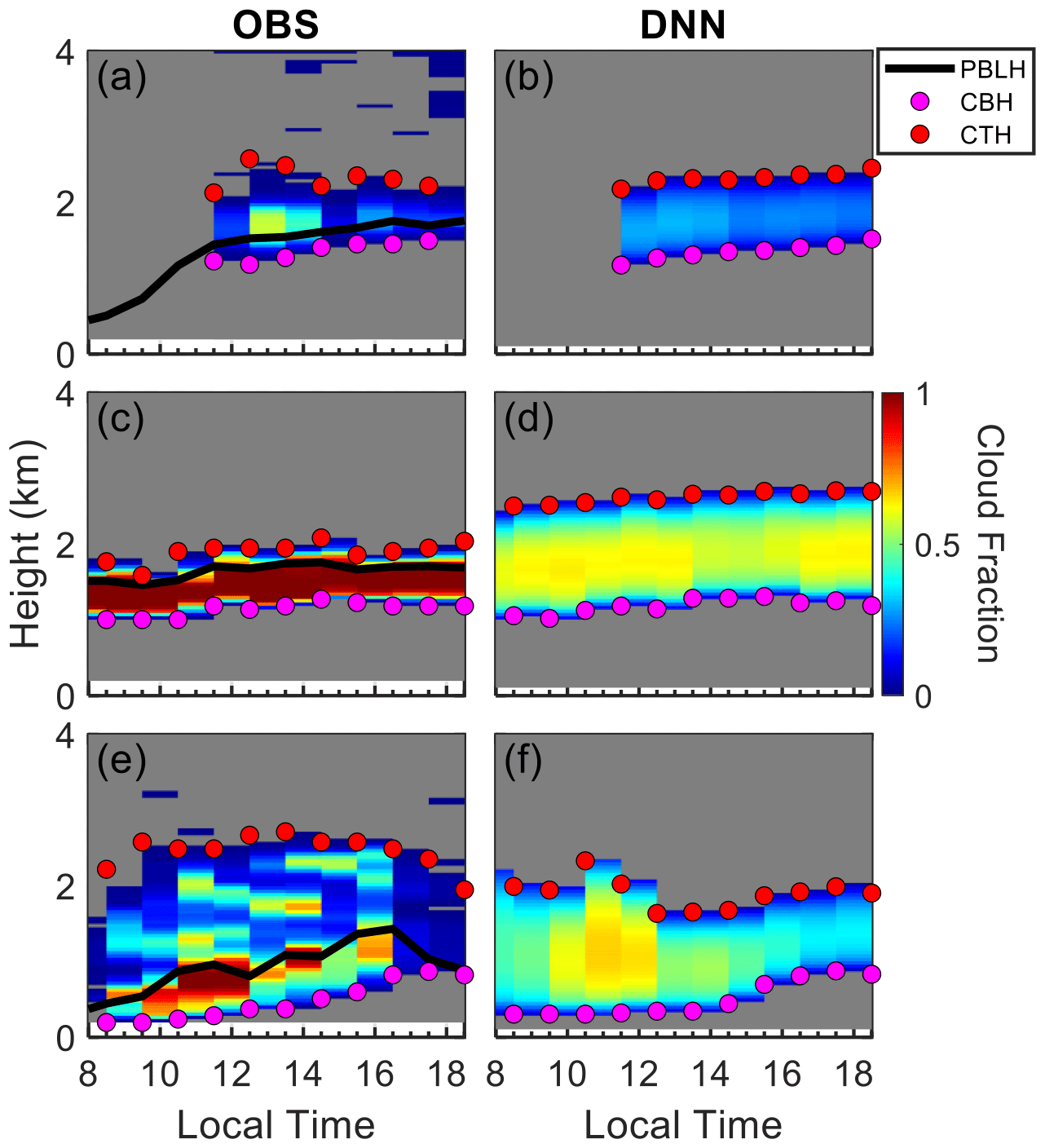
Figure 2 Examples of diurnal cloud fraction profiles for cumulus (a, b), stratiform (c, d), and complex (e, f) cloud structures over the US Southern Great Plains. Observed data (OBS) are shown alongside deep-learning neural network (DNN) simulations. Black lines represent the observed PBL height (PBLH), with the cloud base (CBH) and cloud top height (CTH) marked by pink and red dots, respectively. The color gradient indicates the cloud fraction.

3.4 Calculation of feature importance and performance metrics

To elucidate the significance of each input variable within our deep-learning models, we implement a permutation importance analysis. This robust, model-agnostic technique assesses each feature's influence on the model's predictive accuracy, which is crucial for assessing DNNs (Date and Kikuchi, 2018; Altmann et al., 2010). In this study, the permutation importance method differs slightly for each module within the deep-learning model, based on whether the module's task is regression (cloud-base and fraction-thickness modules) or classification (occurrence module).

For the cloud-base and fraction-thickness modules, which are regression tasks, the mean absolute error (MAE) serves as the performance metric. First, we perform a test run to establish a baseline performance by calculating the MAE of the module using the original, unperturbed validation datasets, which comprise the early-morning sounding, the surface conditions, and the derived variables used as the inputs. Then, for every input feature in the validation set, we disrupt its association with the target cloud fields by shuffling its values across all instances, creating a permutation of the dataset. This is executed while maintaining the original order of the other features. When performing the permutation, we shuffle the entire morning profile for each case without altering the internal height order of values within the profile. This approach ensures that while profiles are permuted across different cases, the sequential structure of height values within each profile remains intact. This method allows us to assess the importance of the profiles as coherent units, rather than disrupting their vertical structures. Furthermore, we re-run the DNN modules with the shuffled feature and all other features intact as inputs and recalculate the MAE with the new outputs. The difference between this new MAE and the baseline MAE represents the feature's importance. To ensure a comprehensive assessment, the permutation and the subsequent MAE calculation are repeated 20 times with different random shuffles for each input feature. The final importance score for each feature is then determined as the mean increase in MAE across these permutations.

For the module of cloud occurrence, which is a classification task, the accuracy score is used as the performance metric. The accuracy score is a measure of the model's overall correctness and is calculated using the formula

$$\begin{array}{}\text{(1)}& \mathrm{Accuracy}={\displaystyle \frac{\mathrm{TP}+\mathrm{TN}}{\mathrm{TP}+\mathrm{TN}+\mathrm{FP}+\mathrm{FN}}},\end{array}$$

where TP (true positives) indicates the number of instances correctly predicted as positive, TN (true negatives) indicates the number of instances correctly predicted as negative, FP (false positives) indicates the number of instances incorrectly predicted as positive, and FN (false negatives) indicates the number of instances incorrectly predicted as negative. After determining the performance metric, other procedures for determining feature importance remain the same for the regression tasks and the classification task.

After determining the importance scores from the test run, to refine the model, features contributing a negligible or negative effect on performance (i.e., importance scores less than zero) are excluded to ensure only beneficial data are used.

Figure 3 illustrates the importance scores from different features obtained using this methodology, underscoring the most influential factors for predicting BLC occurrence, the cloud base, and the thickness and shape of the vertical fraction of BLCs. These factors are ranked from the most important factors to the least important factors. Notably, the importance scores are not computed as a simple sum but are determined by collectively shuffling groups of features and observing the impact on model performance. The BLC trigger for occurrence is a special factor since it is the output of the classification model. The trigger value, which indicates the likelihood of cloud occurrence, is used as an input to obtain the estimations of cloud boundaries and fractions. Sometimes the trigger value hovers around 0.5, indicating uncertainty about the presence of clouds. This situation often corresponds to scenarios like broken clouds or residual clouds, typically associated with relatively small cloud fractions. Incorporating the trigger value as an input for cloud fraction estimation helps the model account for these ambiguous situations, thereby enhancing its ability to estimate the cloud fraction. Specifically, only trigger values greater than 0.5 indicate cloud presence and are used for cloud fraction predictions. While including the trigger value is beneficial for the cloud fraction model, it does not affect the CBH estimation.

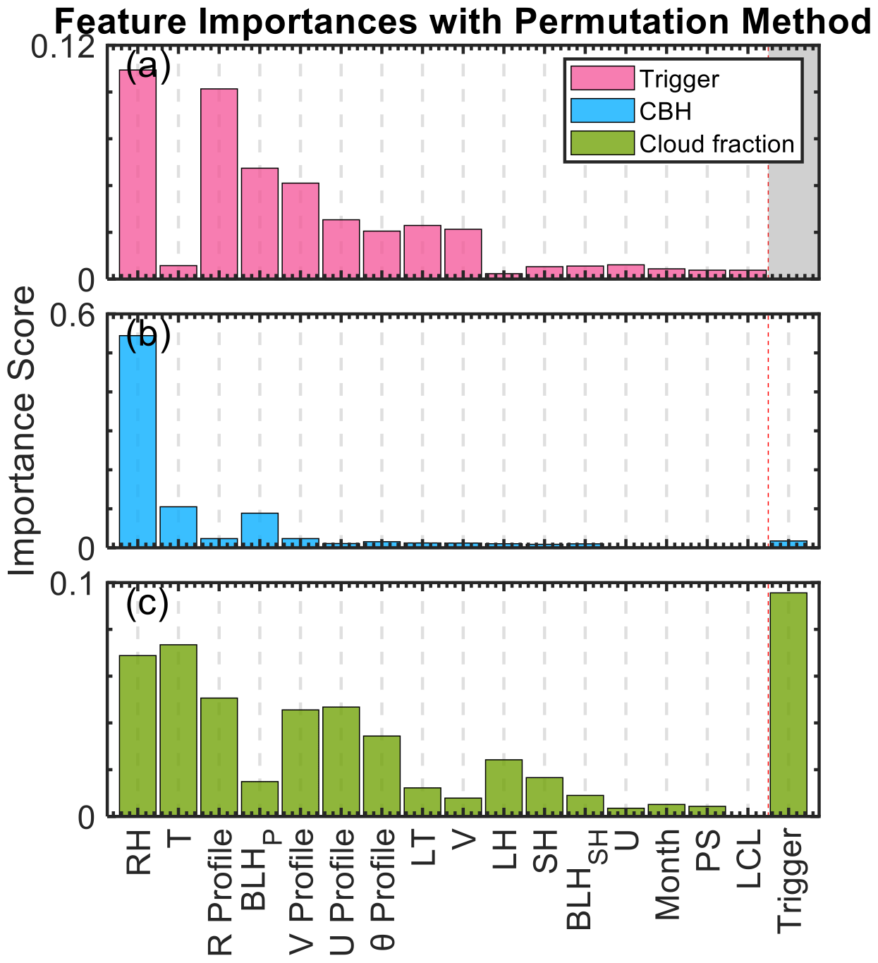
Figure 3 Feature importance scores for predicting cloud occurrence (a), cloud base height (CBH) (b), and cloud fraction (c) in the deep-learning simulations of BLCs. Each panel presents the relative contributions of input features, including month, local time (LT), surface pressure (PS), relative humidity (RH), zonal (U) and meridional (V) wind components, temperature (T), lifting condensation level (LCL), boundary layer height derived from sensible heat (BLH_SH) and parcel methods (BLH_P), sensible heat (SH), latent heat (LH), and morning profiles of relative humidity (R Profile), U wind (U Profile), V wind (V Profile), and potential temperature (θ Profile). These factors are ranked based on their overall importance. The importance scores are calculated with a permutation method and quantify the relative contribution of each feature to the model's predictive accuracy.

In particular, the surface relative humidity (RH), surface air temperature (T), and morning relative-humidity profiles are highly influential in the BLC simulations. This is consistent with previous observational and modeling studies (Zhang and Klein, 2013). Surface RH is a critical factor affecting the occurrence, CBH, and cloud fraction predictions. As they are the input conditions for the DNN modules, the early-morning atmospheric profiles of different meteorological parameters (i.e., RH, temperature, and wind components) exert a notable impact on cloud occurrence detection and the determination of cloud fractions. Surface air temperature is shown to have a substantial effect on cloud fraction, highlighting the sensitivity of cloud simulations to near-surface thermal conditions. Meanwhile, BLH_parcel demonstrates a notable impact, which is understandable since the PBLH is a critical factor for the formation of BLCs, and BLH_parcel provides a good representation of the PBLH. This approach also recognizes the interconnectedness of certain features and their collective contribution to the model's output.

4 Boundary layer cloud simulations by the deep-learning model

4.1 The occurrence of boundary layer clouds

The occurrence of BLC is a multifaceted process influenced by a variety of atmospheric parameters and surface processes. As it is a critical component in the formation of BLCs, we utilize the deep-learning model to identify the BLC trigger using morning meteorological profiles and the observed surface meteorology and fluxes. Figure 4 showcases the model's proficiency in classifying the occurrences (class 1) and non-occurrences (class 0) of BLC during both a training period and an independent period. The classification significantly affects the statistical estimation of cloud fraction, as cloud fraction is set to 0 if the trigger is less than 0.5. The confusion matrices (Luque et al., 2019) for the training period (1998–2016) and for the independent period (2017–2020) display the model's predictive performance. The matrices reveal the counts and percentages of TP, FP, TN, and FN. For the training period, we use a 70 % training and 30 % validation split to ensure model validation and use the validation dataset to generate the statistics. Meanwhile, for the independent period, we use the full dataset for the validation.

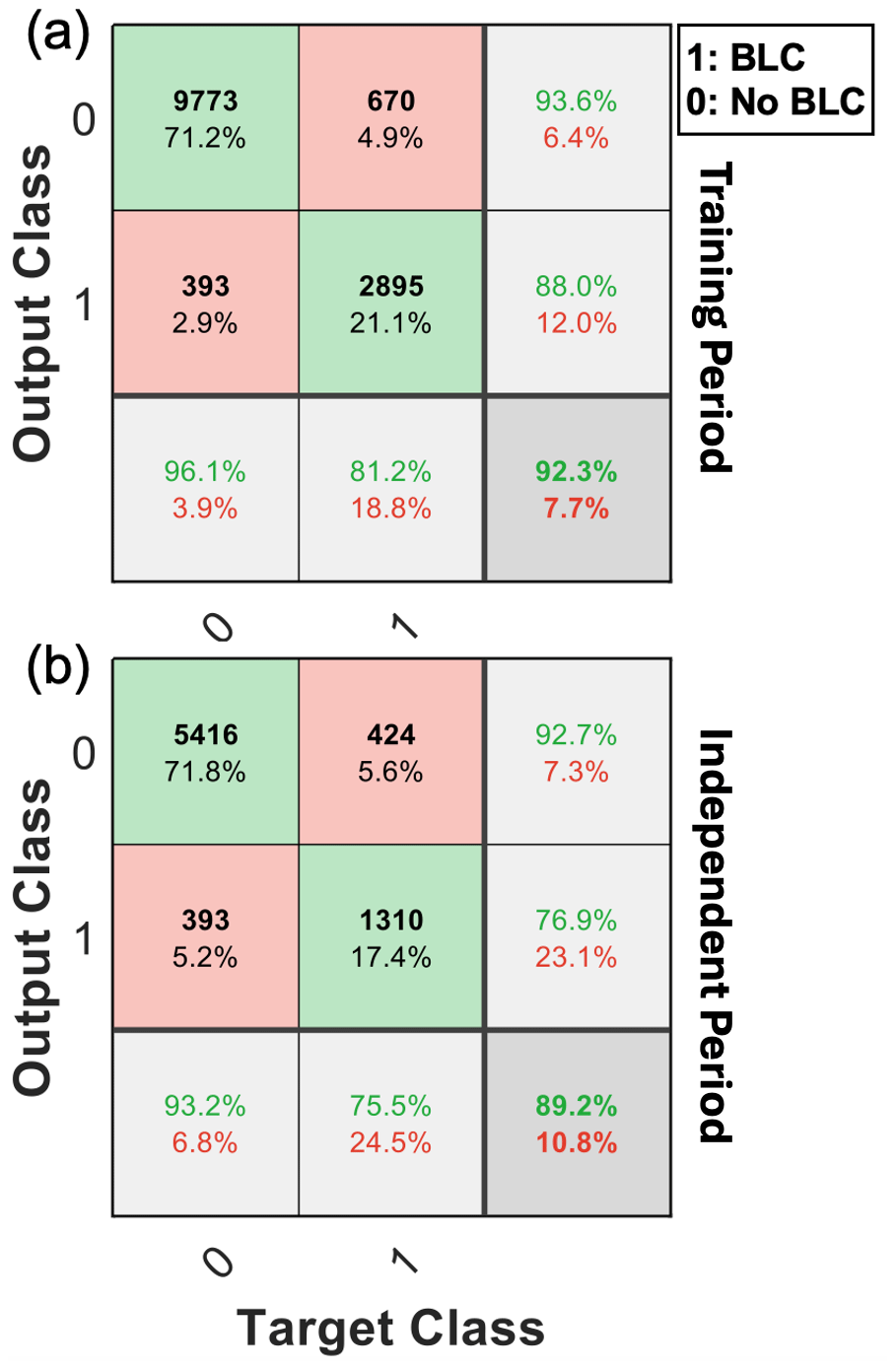
Figure 4 Confusion matrices for the classification performance of the deep-learning model in predicting the occurrence of boundary layer clouds (BLCs) during (a) the training period (1998–2016) and (b) the independent period (2017–2020). The matrices in the training period are calculated using the 30 % of the dataset used for the validation. The matrices with black values display the counts and percentages of true-positive (TP), false-positive (FP), true-negative (TN), and false-negative (FN) predictions. The overall accuracy, precision, and recall scores for each class are also included, demonstrating the model's ability in identifying BLC occurrence.

Figure 4a represents the training period. The validation datasets show high percentages of TN (71.2 %) and TP (21.1 %), indicating that the model is accurate for the period on which it was trained. For the independent period (2017–2020), the model still performs well, with 71.8 % TN and 17.4 % TP (Fig. 4b). However, the rates of FN and FP are slightly higher at 5.6 % and 5.2 %, respectively, which could indicate that the model is slightly less accurate when applied to data beyond its training scope. The table highlights the model's robustness, with an overall accuracy rate of 92.3 % for the training period and a slightly reduced but still substantial rate of 89.2 % for the independent period. Moreover, for the training period, the model achieved a high precision of 88.1 % and a recall of 81.2 %. For the independent period, the precision and recall remained reasonably high at 76.9 % and 75.6 %, respectively, demonstrating the model's effective generalization to new data. These metrics demonstrate the model's predictive capabilities and reliability for both the training and independent periods.

Figure 5 further compares the diurnal frequency of BLC occurrence between observations (OBS) and the DNN predictions for different seasons. The BLC's strong diurnal pattern is well captured by the model, as BLC development peaks between 12:00–16:00 local time, aligning closely with observed frequencies. Among the different seasons, the model is notably effective in simulating the pronounced diurnal cycle of summer clouds, which are typically influenced by local convection. Conversely, the winter season exhibits a weaker diurnal pattern, likely linked to the diminished surface fluxes. The DNN tends to overestimate BLC presence in the early morning, especially for the winter season. The overall alignment between observations and the DNN module represents the model's capability to capture the diurnal patterns of BLC formation and development. Determining the occurrence of BLC lays the foundation for the integrated simulations of BLC features.

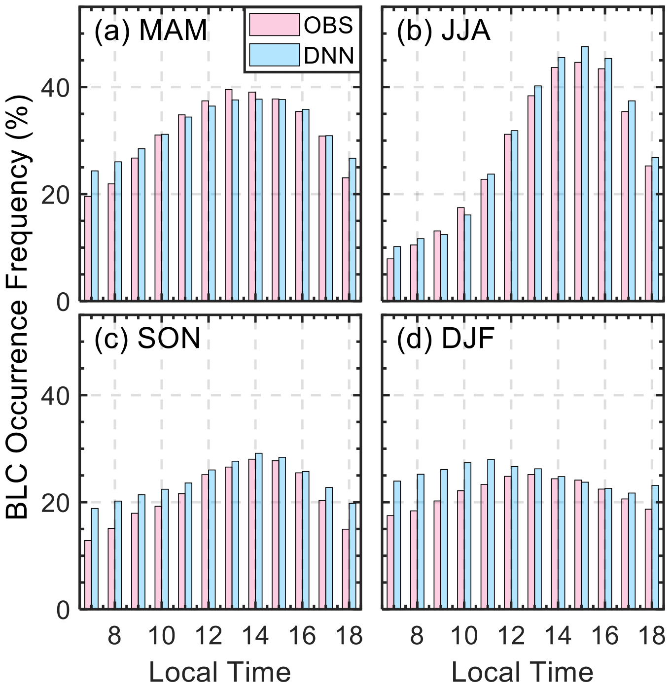
Figure 5 Bar graph comparison of the occurrence frequency of boundary layer cloud (BLC) between the observed frequency (OBS, red) and the frequency predicted by the deep-learning neural network (DNN, blue) at different local times of the day during each season: (a) MAM (spring), (b) JJA (summer), (c) SON (fall), and (d) DJF (winter).

4.2 Cloud boundaries and fraction

A key aspect of cloud modeling involves the accurate simulation of the cloud boundaries and fraction, which are indicative of a cloud's vertical extent and fractional coverage at different height levels. Our deep-learning model demonstrates capabilities to predict these key attributes of BLC.

Figure 6 offers comparisons between observed values and predictions by the DNN for CBH, CTH, and cloud fraction. As in Sect. 4.1, these comparisons are presented for both the training period (Fig. 6a, c, e, based on validation datasets) and an independent period (Fig. 6b, d, f), revealing the model's ability to generalize beyond its initial training data. The DNN model demonstrates remarkable performance in simulating the cloud base, boasting a correlation coefficient surpassing 0.9 and an MAE below 0.15 km. Conversely, the model encounters challenges in CTH prediction, evidenced by a lower correlation of about 0.5 and a significantly higher MAE of between 0.8 and 0.9 km, aligning with case studies in Fig. 2.

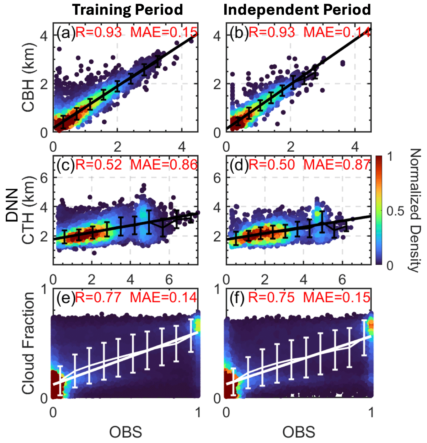
Figure 6 Scatter density comparison between the observed (OBS) and the values predicted by the deep-learning neural network (DNN) for cloud base height (CBH), cloud top height (CTH), and cloud fraction during the training period (a, c, e) and an independent period (b, d, f). Note that the BLC is segmented into 10 layers, yielding 10 separate cloud fraction values per BLC instance for analysis. The correlation coefficient (R) and mean absolute error (MAE) are indicated for each comparison. The color scale represents the normalized density of data points. Each solid line shows a linear regression and each error bar denotes the standard deviation.

The discrepancy in accurately simulating CBH and CTH may stem from two main factors. Firstly, observed CBH determinations are generally more precise due to the effectiveness of laser-based methods (Pal et al., 1992), while observed CTH estimations often suffer from reduced accuracy, which is partly attributed to signal attenuation issues (Clothiaux et al., 2000). For observed shallow cumulus, the cloud top is often contaminated by insect signals, further complicating accurate CTH measurements (Chandra et al., 2010). Secondly, our DNN simulations are developed from the perspective of cloud–land coupling and primarily utilize the surface meteorology. This can introduce inherent limitations, as the tops of many clouds may be affected by free-troposphere conditions despite the presence of a coupled base, potentially leading to gaps in the DNN's ability to accurately define and estimate the cloud top.

A comparison of cloud fraction between observations and the DNN model is presented in Fig. 6e–f to examine the model's capability to simulate the vertical distribution of cloud fraction. The scatterplots comparing observed and modeled cloud fractions at individual levels in cloudy scenarios show satisfactory correlation, with an R value exceeding 0.77 and an MAE of around 0.15. Nevertheless, the DNN model tends to underestimate the peak cloud fraction: it ranges up to ∼ 0.8, whereas the full range (0–1) is observed. This underestimation is intrinsically linked to the model's simulation of cloud boundaries, as both the cloud-fraction and cloud-base modules operate in tandem. For stratiform clouds, observational data typically exhibit a relatively uniform vertical extent, with cloud fractions of close to unity at the central height, whereas the DNN model tends to generate a broader, more attenuated profile with a reduced maximum cloud fraction at the center. This points to a need to refine the model's ability to replicate the pronounced peak cloud fractions characteristic of stratiform cloud profiles.

The diurnal patterns of cloud base and top height captured through daily profiles showcase the model's adeptness at simulating the temporal changes in cloud positions for all BLCs, the cumulus regime, and the stratiform regime (as shown in Fig. 7). These profiles, derived from both observational data and DNN outputs, include shaded regions representing the variability (1 standard deviation) around the average heights. Cumulus clouds exhibit a marked diurnal cycle, whereas stratiform clouds typically maintain relatively constant cloud boundaries and show smaller variations throughout the day. The mean and standard deviation of the cloud base show close alignment between the observed and the simulated data for different cloud regimes. In contrast, while the mean cloud top heights follow a similar diurnal trend in both cases, the observed data exhibit more pronounced variabilities compared to the relatively small variabilities in the DNN simulations.

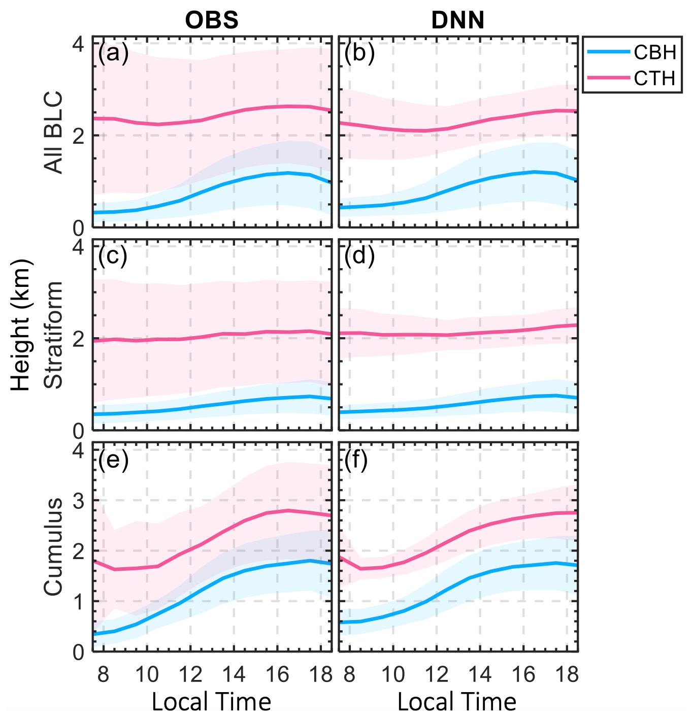
Figure 7 Diurnal profiles of cloud base height (CBH) and cloud top height (CTH) as determined from observations (OBS) and deep-learning simulations for all BLCs (a–b), stratiform clouds (c–d), and cumulus (e–f). The shaded areas represent the variability (1 standard deviation) around the mean heights.

Figures 6 and 7 collectively demonstrate the model's ability to simulate cloud boundaries and fractions within BLC. It reliably captures the CBH yet encounters challenges in accurately representing cloud top heights and peak cloud fractions on an individual basis. These constraints are somewhat expected, given that even very fine-scale models struggle to entirely capture the vertical extent of clouds, as evidenced by large-eddy simulations and convection-permitting models (Y. Zhang et al., 2017; Gustafson et al., 2020; Bogenschutz et al., 2023). In addition to the discussion of deep-learning models, we also acknowledge the role of mixed-layer (single-column) models in representing boundary layer processes (Lilly, 1968; Pelly and Belcher, 2001; Clayson and Chen, 2002; Zhang et al., 2005, 2009; De Roode et al., 2014). Mixed-layer models have several advantages: they are inherently grounded in physical principles and are readily integrated into many large-scale models. These models are effective at capturing the diurnal evolution of the PBL given an initial state and time series of surface fluxes. However, the DNN approach offers distinct benefits that complement this theoretical approach. DNNs might be able to capture complex, nonlinear relationships between various controlling factors and the cloud fraction. These may be difficult to capture using single (for overcast stratocumulus-topped mixed layer) or multiple (for broken trade cumulus clouds) mixed-layer models, which are still subject to assumptions, e.g., on entrainment processes. By training on large observational datasets, DNNs can learn from real-world examples, potentially identifying patterns and relationships not explicitly encoded in physical models.

5 Application of the deep-learning model

5.1 Integration with reanalysis datasets

As shown in Sect. 4, the deep-learning model can take conventional meteorological observations (i.e., morning SONDE data and surface conditions) as inputs to simulate the BLC as outputs, producing a reasonably good agreement with the observed vertical structures of BLCs. In potential applications, we may treat it as an “emulator” of the observed relationships between input and output variables. Here we present an example of integrating the deep-learning model with ERA5 and MERRA-2 to simulate BLC, with early-morning profiles and surface conditions from the reanalysis used as input. Here we ask, if the inputs are treated as “reality”, what would the expected resulting cloud fraction simulated by the deep-learning model, an observation-based emulator, be?

Following these thoughts, Fig. 8 contrasts diurnal cloud-fraction patterns from the observational data with the deep-learning model predictions averaged over all conditions across seasons and years. Figure 8a and b present the observed cloud fractions and those simulated by the deep-learning model using ARM data as inputs, respectively. Panels c and e show the cloud fractions directly extracted from ERA5 and MERRA-2 reanalysis datasets, while panels d and f illustrate the cloud fraction simulated by the deep-learning model using inputs from ERA (ERA_DNN) and MERRA (MERRA_DNN) reanalysis data. Observing fluctuations in surface-temperature and humidity data in ERA5 for this region, we smoothed the ERA5 surface-air-temperature and humidity data with a ±1 h window to mitigate potential variability from assimilation before using them as input for the DNN modules. To eliminate sampling biases in the comparison, we averaged only those samples for which both observations and reanalysis are concurrently available.

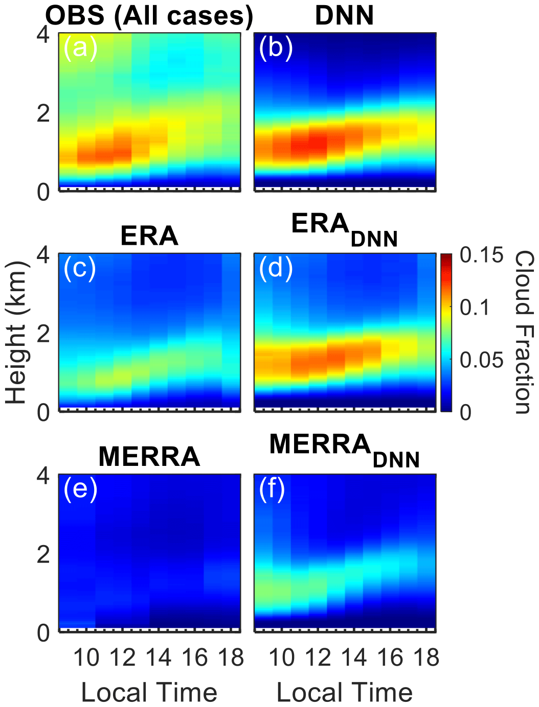
Figure 8 Color-shaded areas demonstrate the observed and simulated diurnal variation in cloud fraction for all cases. Panel (a) shows the observed cloud fraction (OBS), while panel (b) illustrates the cloud fraction simulated by the deep-learning neural networks (DNNs) using ARM observational data as inputs. (c, e) Cloud fractions directly extracted from the ERA and MERRA reanalysis datasets, respectively. (d, f) Cloud fractions simulated by the DNN model using ERA (ERA_DNN) and MERRA (MERRA_DNN) data as inputs.

Note that here we adopt the deep-learning model as a complementary tool rather than as a replacement for any existing cloud representations in reanalysis data. The DNN outputs serve a diagnostic purpose, identifying biases in BLCs and aiding in understanding deficiencies within the reanalysis data.

The DNN simulations with ARM observations as inputs align closely with the ARM-observed cloud fraction profiles within the 0–2 km range, reflecting the model's ability to capture land-coupled clouds. As this model is designed for diagnosing land-coupled clouds, the model does not simulate decoupled clouds, which often have bases occurring above 2 km (Su et al., 2022). Original cloud data directly from reanalysis show significant underestimations of BLC fractions, which are particularly evident in MERRA-2. The application of the deep-learning model using reanalysis data as inputs enhances cloud fraction estimations compared to the original cloud data directly from reanalysis, demonstrating the DNN model's strength in simulating BLC. Given that the DNN model specializes in simulating BLC, when utilizing reanalysis data, the set of cloud profiles that are decoupled (i.e., for the cloud layers above the BLC tops or the clouds rooted above the PBL) are preserved as they are in the original datasets.

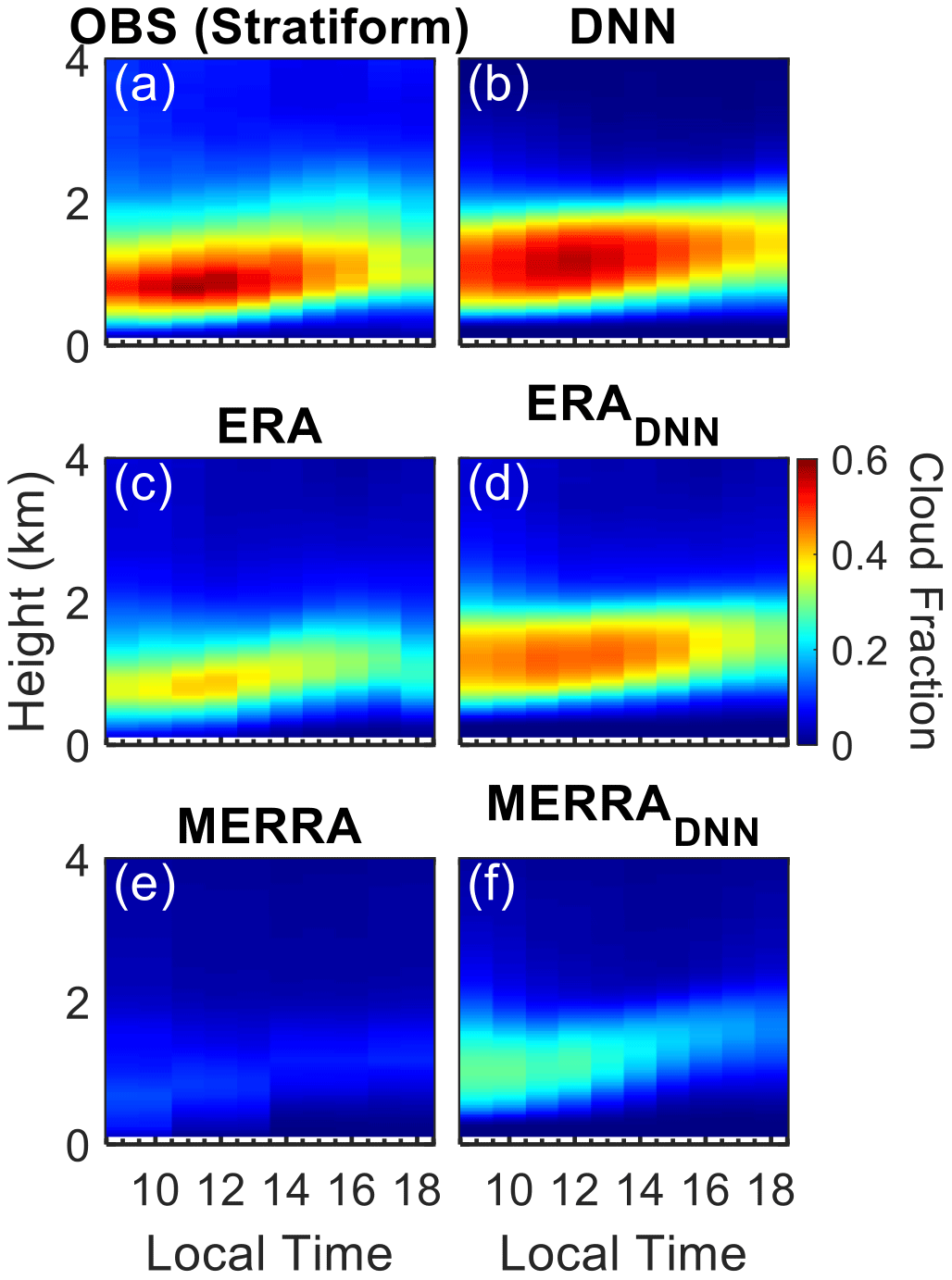
Furthermore, Fig. 9 provides a detailed examination of stratiform clouds, utilizing the same comparative approach as in Fig. 8. The observed stratiform clouds display a layered structure with expansive coverage and maximum cloud fractions typically exceeding 0.6. The DNN model using ARM data as inputs reproduces these observed characteristics fairly well, albeit with minor overestimations in cloud vertical extent. Conversely, the original ERA5 and MERRA-2 stratiform cloud data exhibit limitations, particularly in underestimating the cloud fraction. The integration of the DNN model with reanalysis data as inputs enhances the estimations of stratiform cloud fractions, as depicted in the heatmaps of Fig. 9, which showcase an improved agreement with observational data and underscore the enhancement potential of cloud fraction simulations using reanalysis datasets.

Figure 9 Same as Fig. 8 but for stratiform clouds.

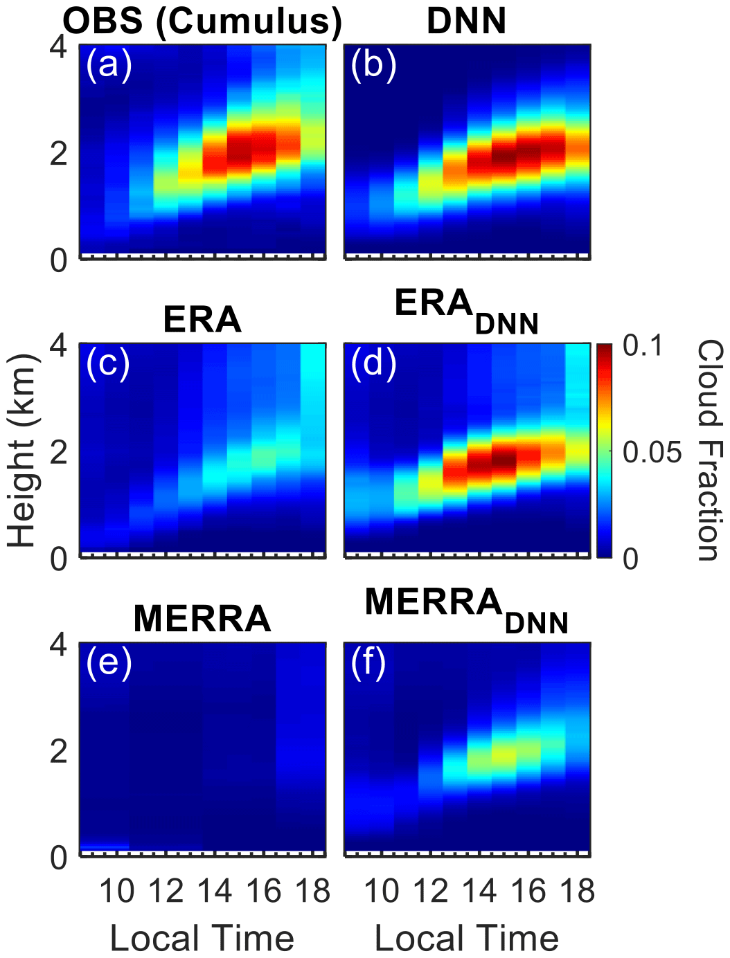
In addition, Fig. 10 extends the comparative study to cumulus clouds. Cumulus clouds pose significant challenges to modeling and parameterization, partly due to their typically small spatial extent compared to the model resolution: they often span a few hundred meters to several kilometers in size (Y. Zhang et al., 2017; Tao et al., 2021; Bogenschutz et al., 2023; Gustafson et al., 2020). In line with expectations, the original ERA5 and MERRA-2 cloud fields exhibit significant biases in representing cumulus clouds when compared to observational data. In contrast, the DNN model with ARM data as inputs achieves commendable success in capturing the diurnal variability of cumulus clouds, including the cloud base, vertical extension, and cloud fraction, by leveraging local convective signals derived from surface meteorology data. When the DNN model is integrated with ERA5 as inputs, the estimation of vertical cloud fields of cumulus significantly improves. However, the original MERRA-2 data tend to overlook the majority of cumulus clouds, and they are still significantly underrepresented after the application of the DNN, suggesting that additional biases in the input variables such as meteorological factors may contribute to this discrepancy.

Figure 10 Same as Fig. 8 but for cumulus.

The integration of deep learning with ERA5 and MERRA-2 reanalysis datasets leads to notable refinement in the simulation of BLC and achieves more accurate estimations of cloud fraction for both stratiform and cumulus clouds.

5.2 Applying deep learning for bias attribution in cloud simulation

We further examine the disparities that remain in cloud fraction simulations within reanalysis datasets despite the integration of deep-learning models (as shown in Figs. 8–10), which indicate persisting meteorological biases. Deep learning is utilized to quantify and attribute these biases for BLC simulations.

Figure 11 offers a comparative analysis of vertical cloud-fraction profiles for both stratiform and cumulus clouds. It presents cloud fraction directly taken from reanalysis data (RD), including ERA5 and MERRA-2, and their corresponding deep-learning-informed simulations. While the application of deep learning to use reanalysis data as inputs (RD_DNN) yields improvements, remaining cloud biases are evident, particularly in MERRA-2. Acknowledging the significant influence of the surface RH on BLC simulations (as indicated by Fig. 3e), we refine the inputs into the DNN model by replacing the reanalysis surface RH with the ARM-observed surface RH (the resulting model output is labeled as RD_DNN-RH). This modification leads to a much better simulation for MERRA-2, closing the gap with observational data, especially for stratiform clouds. For ERA5, RD_DNN-RH and RD_DNN show negligible differences for cumulus clouds, but for stratiform clouds, RD_DNN-RH also exhibits a reduced bias. These refined profiles of cloud fraction attest to the benefits of using the observed surface moisture data as input, confirming its important role in achieving a more accurate representation of BLC.

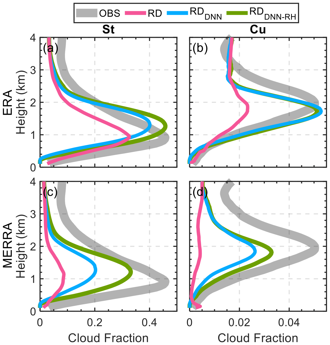
Figure 11 Vertical profiles of cloud fraction for stratiform (St) and cumulus (Cu) scenarios over the US Southern Great Plains. Panels (a) and (b) display ERA reanalysis data comparisons, while panels (c) and (d) show MERRA reanalysis data comparisons. The observed cloud fractions (OBS) are represented by the shaded grey area, illustrating the averaged cloud coverage recorded by field observations. The original reanalysis data (RD) are indicated in pink, indicating the baseline cloud-fraction profiles as simulated by the reanalysis. The RD_DNN profiles in blue depict the new simulation results after applying the DNN models to the reanalysis data used for boundary layer cloud (BLC) simulation. The RD_DNN-RH profiles in green show the simulation results when the surface relative humidity (RH) from the reanalysis data is replaced with observed values, indicating the impact of accurate surface moisture representation on cloud fraction simulations.

With this methodology, we may further dissect the bias in cloud fraction simulations, attributing it to various meteorological factors and the parameterization schemes used within ERA and MERRA reanalysis datasets:

$$\begin{array}{}\text{(2)}& {\displaystyle }\begin{array}{rl}\text{Bias due to parameterization}& =\left|\mathrm{RD}-\mathrm{OBS}\right|\\ & -\left|{\mathrm{RD}}_{\mathrm{DNN}}-\mathrm{OBS}\right|\end{array}\text{(3)}& {\displaystyle }\begin{array}{rl}\text{Bias due to surface RH}& =\left|{\mathrm{RD}}_{\mathrm{DNN}}-\mathrm{OBS}\right|\\ & -\left|{\mathrm{RD}}_{\text{DNN-RH}}-\mathrm{OBS}\right|,\end{array}\end{array}$$

where RD and OBS are the cloud fractions taken directly from reanalysis data and observations, respectively. RD_DNN and RD_DNN-RH are defined the same as above. To get a representative value, these biases are layer averaged from 0–4 km at different local times and then normalized by the observed mean cloud fraction, offering a climatological perspective on the discrepancies between observed and simulated data across seasons and years. For Eq. (2), we assume that the climatology of observations used as input to the DNN model (OBS_DNN) matches the observed cloud-fraction climatology (i.e., OBS_DNN≈ OBS), which is demonstrated in Figs. 9–11. Therefore, we exclude the term representing the difference between the DNN-predicted observations and the actual observations. This assumption justifies our approach by ensuring the input observations align with the observed cloud fraction in equations.

We get the bias attributable to different meteorological factors and parameterization schemes in the ERA5 and MERRA-2 datasets, respectively (Fig. 12). Each bar indicates the normalized bias contributed by factors such as morning meteorological profiles, surface pressure, surface fluxes, various surface meteorology variables, and parameterization schemes. Notably, parameterization stands out as a significant contributor to bias, accounting for 14.45 % and 19.05 % of the discrepancy in stratiform clouds between observations and ERA5 and between observations and MERRA-2, respectively. For cumulus clouds, the parameterization biases are more pronounced, contributing 22.23 % and 30.94 % of the discrepancy for ERA5 and MERRA-2, respectively.

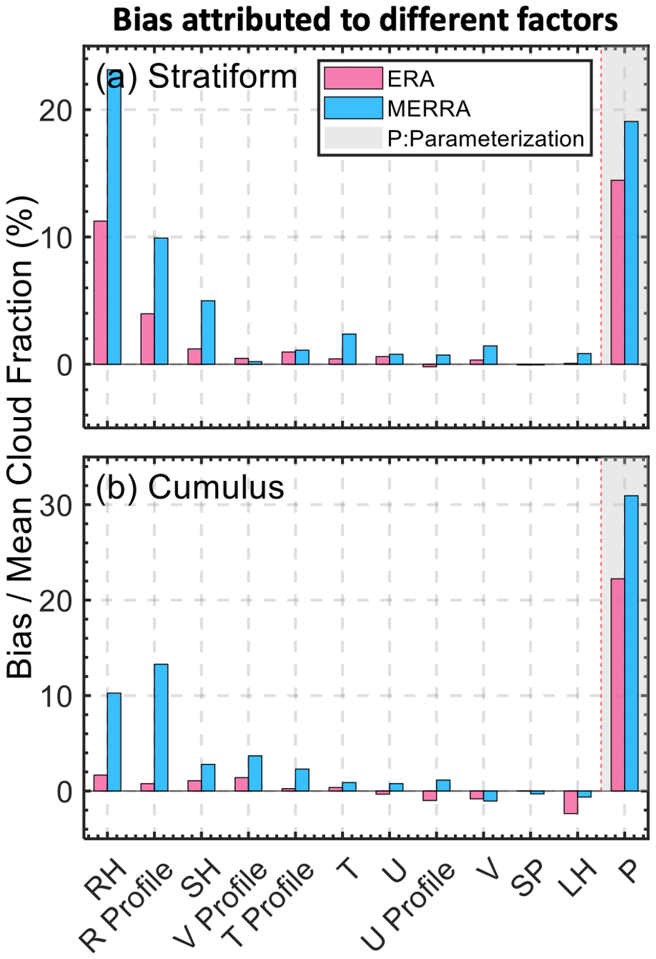
Figure 12 Attribution of the bias in cloud fractions between observations and reanalysis to various meteorological factors and parameterization schemes for stratiform (a) and cumulus (b) cloud scenarios. The bars represent the normalized bias (bias divided by mean cloud fraction) contributed by each of the following factors: surface relative humidity (RH), relative humidity profile (R Profile), meridional wind profile (V Profile), temperature profile (T Profile), zonal wind profile (U Profile), surface pressure (SP), sensible heat flux (SH), latent heat flux (LH), and parameterization (P). All profiles were taken in the morning (06:00 LT). Light blue bars indicate biases identified in the ERA reanalysis dataset, while pink bars represent biases in the MERRA reanalysis dataset. “P” denotes biases attributed specifically to the parameterization within the reanalysis models. This analysis uses the DNN to discern the impact of each factor (ranked from highest to lowest) on the discrepancy in cloud fraction estimates between observations and reanalysis models.

In addition to parameterization, RH, RH profiles, and sensible heat are identified as major factors contributing to the differences between observations and reanalysis data. For instance, aligning MERRA-2's RH with the observed surface RH could potentially reduce the bias by 23.13 % for stratiform and 10.26 % for cumulus clouds. Meanwhile, the surface RH and morning RH profiles in ERA5 yield 11.25 % and 3.96 % of the bias for stratiform clouds. The bias between ERA5 and observed cumulus clouds is largely driven by parameterization, which suggests that employing the DNN model with ERA5 can lead to a more accurate simulation of cumulus clouds.

The detailed bias attribution analysis facilitated by the deep-learning model elucidates the individual impacts of meteorological factors on the discrepancies in cloud fraction between observations and reanalysis data. It underscores the necessity for more accurate humidity data within reanalysis datasets to refine BLC simulations. Furthermore, this deep-learning approach illuminates pathways for guiding the directions to improve parameterization of boundary layer convection.

6 Summary

This study has developed a deep-learning model to estimate the evolution of BLCs over the SGP. The model utilizes over 2 decades of meteorological data to simulate BLC formation and characteristics, including the occurrence of BLCs, cloud boundaries, and vertical structures of the cloud fraction. As this model is built based on the perspective of cloud–land coupling, the DNN approach demonstrates the capability to diagnose land-coupled convective systems from early-morning sounding and surface conditions. The DNN model is built on cloud–land interactions and serves as testimony to the coupling between BLCs and the land surface. The proficiency and reliability of the DNN model are evident in its robustness during both the training period and the subsequent independent periods. The deep-learning model addresses the simulation of cloud vertical structure, which is one of the key challenges in physics-based large-scale models. It should be noted that the current DNN model cannot produce detailed cloud microphysics and turbulence information. We propose using the DNN model alongside traditional physical models to obtain comprehensive information on BLCs.

The application of this model to reanalysis datasets like ERA5 and MERRA-2 resulted in enhanced cloud field estimations for stratiform clouds and cumulus and an accurate vertical structure of clouds in terms of the climatology, indicating that it is a promising diagnostic tool for improving weather forecasting and climate modeling. The deep-learning model notably addresses the limitation on cumulus simulations using reanalysis data. Meanwhile, this approach is much more cost-effective compared to traditional parameterizations and schemes at various scales, as it can simulate 2 decades of BLCs with vertical information over the SGP within 1 min using a single GPU node.

In addition to BLC simulations, the deep-learning model developed in this study was also used to attribute discrepancies between observational data and reanalysis datasets to different meteorological factors. Besides parameterization, surface RH, morning RH profiles, and surface sensible heat are the three major factors that led to the mismatches in BLC representation in ERA5 and MERRA-2. These findings underscore the importance of incorporating more accurate humidity information into reanalysis datasets; this is crucial for refining BLC simulations. This analysis also sheds light on the necessity to update reanalysis datasets with improved parameterization of boundary layer convection.

Moving forward, future work is warranted to test this diagnostic tool and extend it to different synoptic patterns over a large region, as the tool can be integrated into both multiple-scale models and reanalysis data. However, several challenges need to be addressed to achieve this. One significant limitation is the lack of high-quality, detailed observations of clouds and radiosonde profiles globally. This scarcity of data can hinder the model's ability to generalize effectively across different regions. To overcome this, there are several potential strategies. First, transfer learning techniques can help adapt a model trained in one region to other regions with limited data. Integrating data from global observational networks (i.e., ARM) can also create a more diverse and representative training dataset that captures a wider range of atmospheric conditions and cloud characteristics. Meanwhile, leveraging satellite data can provide broader coverage and enhance the robustness of the model. We plan to explore these approaches in future work to enhance the model's performance and applicability on a global scale.