the Creative Commons Attribution 4.0 License.
the Creative Commons Attribution 4.0 License.
 | 27 Aug 2024
Mixed-precision computing in the GRIST dynamical core for weather and climate modelling
Siyuan Chen
Yiming Wang
Zhuang Liu
Xiaohan Li
Wei Xue
Atmosphere modelling applications are becoming increasingly memory-bound due to the inconsistent development rates between processor speeds and memory bandwidth. In this study, we mitigate memory bottlenecks and reduce the computational load of the Global–Regional Integrated Forecast System (GRIST) dynamical core by adopting a mixed-precision computing strategy. Guided by an application of the iterative development principle, we identify the coded equation terms that are precision insensitive and modify them from double to single precision. The results show that most precision-sensitive terms are predominantly linked to pressure gradient and gravity terms, while most precision-insensitive terms are advective terms. Without using more computing resources, computational time can be saved, and the physical performance of the model is largely kept. In the standard computational test, the reference runtime of the model's dry hydrostatic core, dry nonhydrostatic core, and the tracer transport module is reduced by 24 %, 27 %, and 44 %, respectively. A series of idealized tests, real-world weather and climate modelling tests, was performed to assess the optimized model performance qualitatively and quantitatively. In particular, in the long-term coarse-resolution climate simulation, the precision-induced sensitivity can manifest at the large scale, while in the kilometre-scale weather forecast simulation, the model's sensitivity to the precision level is mainly limited to small-scale features, and the wall-clock time is reduced by 25.5 % from the double- to mixed-precision full-model simulations.
- Article
(10619 KB) - Full-text XML
- BibTeX
- EndNote


Increasing model resolution is an effective approach to enhancing atmosphere model forecast accuracy (Bauer et al., 2021; Benjamin et al., 2019; Yu et al., 2019). Highly accurate, efficient, stable, and scalable global dynamical cores have been widely pursued over the past 2 decades (e.g. Tomita and Satoh, 2004; Harris and Lin, 2012; Skamarock et al., 2012; Zängl et al., 2015; Wedi et al., 2020; Sergeev et al., 2023; Zhang et al., 2023). Doubling the horizontal resolution with a fixed vertical resolution leads to an increase in computational amount by a factor of ∼23, a significant challenge in terms of computational cost and energy consumption.
Operational weather and climate forecasting is a field where the dual demands of accuracy and computational efficiency converge, necessitating both quality and speed. In the context of high-resolution mesoscale forecasting, which operates on scales of a few kilometres, computational efficiency itself implies forecast accuracy. Faster models enable more frequent forecast-assimilation cycles and the use of larger ensemble sizes within the constraints of finite computational resources. To tackle these computational hurdles, efforts have concentrated on enhancing the efficiency of numerical models. Progress such as field-programmable gate arrays (FPGAs) and heterogeneous computing (e.g. Gan et al., 2013; Yang et al., 2016; Fu et al., 2017; Gu et al., 2022; Taylor et al., 2023), alongside compiler optimizations (e.g. Santos et al., 2024), has demonstrated significant potential in accelerating Earth system models.
Conventional weather/climate model development has typically relied on double-precision (64 bit) floating points. The transition from double- to single-precision (32 bit) or even half-precision floating-point arithmetic presents an intriguing avenue for enhancing computational efficiency (Düben et al., 2014). Single-precision computation unveils several compelling advantages, especially when confronted with the memory wall (Abdelfattah et al., 2021; Fornaciari et al., 2023; Brogi et al., 2024). Beyond the alleviation of memory constraints, single-precision arithmetic promises three distinct benefits: accelerated arithmetic operations, improved cache hit rates, and reduced inter-node data communication (Baboulin et al., 2009; Düben and Palmer, 2014; Düben et al., 2015; Váňa et al., 2016; Nakano et al., 2018). The benefits highlighted illustrate the capability of single-precision computation to boost computational efficiency in high-performance computing tasks, especially within the realm of large-scale weather and climate simulations where computational expenses are significant.
However, a wholesale migration from double- to single-precision computing may not always yield beneficial outcomes. This has led to the exploration of precision-sensitive model components and/or physical scales in Earth system modelling (e.g. Thornes et al., 2017; Nakano et al., 2018; Chantry et al., 2019; Maynard and Walters, 2019; Cotronei and Slawig, 2020). Single-precision algorithms may struggle to converge or achieve the required precision when tackling intricate fluid dynamics simulations. In certain scenarios, single-precision computations can also result in floating-point under-/overflow (Váňa et al., 2016; Cotronei and Slawig, 2020). Additionally, physical parameterization schemes in atmospheric models may amplify grid-scale oscillations when executed in a pure single-precision mode (Váňa et al., 2016). Therefore, it becomes imperative to identify the specific algorithms within the modelling framework that are sensitive to the precision level.
Previous studies have made notable progress. A pivotal study by Váňa et al. (2016) explored the reduction in almost all real-number variables in the Integrated Forecasting System (IFS) of the European Centre for Medium-Range Weather Forecasts (ECMWF) from 64 bits to 32 bits. Results revealed that reducing precision did not significantly compromise the model's accuracy, while it considerably reduced the computational burden by a factor of ∼40 %. Based on the dynamical core of the Nonhydrostatic Icosahedral Atmospheric Model (NICAM), Nakano et al. (2018) witnessed an undesirable wavenumber-5 structure when completely using single-precision computing. This abnormal wave growth was traced back to the errors in the grid cell geometry calculations. By using double precision for only necessary parts in the dynamical core and single precision for all other parts, the model successfully simulated the baroclinic wave growth and achieved a ∼46 % reduction in runtime. Based on the Yin–He global spectral model, Yin et al. (2021) used a single-precision fast spherical harmonic transform to conduct a 10 d global simulation and a 30 d retrospective forecasting experiment. Their simulations reproduced the major precipitation events over southeastern China. The single-precision fast spherical harmonic transform may lead to a reduction in runtime by ∼25.28 % without significantly affecting the forecasting skill. Cotronei and Slawig (2020) converted the majority of the computations within the radiation component of the ECMWF Hamburg Model (ECHAM) to single precision, resulting in a 40 % reduction in the runtime of the individual component. The obtained results were comparable to those achieved with double precision. Banderier et al. (2024) indicated that employing single precision for regional climate simulations can significantly reduce computational costs (∼30 %) without significantly compromising the quality of model results.
While these studies have demonstrated various ways of precision optimization, certain limitations remain. First, some studies focused on a complete transition to single precision, potentially overlooking the precision-sensitive components, and lacked a discussion of optimization strategies. Moreover, the applicability of mixed precision in global climate simulations remains to be validated. Furthermore, because of the diversity of numerical models and algorithms, encompassing grid systems and solver techniques, these differences may lead to model-specific precision sensitivity. Certain algorithms may remain amenable to single-precision computations, while others necessitate the use of double precision for stability and accuracy. These gaps in the literature underscore the need for the present research to explore precision sensitivity and to test reduced-precision computing for both weather and climate simulations.
In this study, we explored the strategies of mixed-precision computing in the dynamical core of the Global–Regional Integrated Forecast System (GRIST; Zhang et al., 2019, 2020). GRIST is a unified weather–climate model system designed for both research and operational modelling applications. Through a detailed implementation by modifying certain parts of the original (double-precision) dynamical core to support single precision, a significant reduction in the computational burden has been achieved without sacrificing the solution accuracy, stability, and physical performance. This has been validated based on a series of numerical tests ranging from idealized to real-world flow.
The remainder of this paper is organized as follows. Section 2 introduces the GRIST model, presents the mixed-precision optimization strategies and code modifications, and highlights the key equation terms sensitive to precision. Section 3 examines the computational performance of mixed-precision computing. Section 4 evaluates the physical performance of mixed-precision computing in a series of test cases. The discussion and conclusion are given in Sects. 5 and 6, respectively.
1.1 GRIST
The GRIST dynamical core employs layer-averaged governing equations based on the generalized hybrid sigma–mass vertical coordinate and a horizontal unstructured grid, allowing for a switch between the hydrostatic and nonhydrostatic solvers (Zhang, 2018; Zhang et al., 2019, 2020). Prognostic variables are arranged in a hexagonal Arakawa C-grid approach. The hydrostatic solver is fully explicit, based on the Runge–Kutta integrator and the Mesinger forward–backward scheme. The nonhydrostatic solver employs a horizontally explicit–vertically implicit approach. There is no time splitting in the integration of the dry dynamical core (dycore hereafter), while the tracer transport module is time split from the dycore and supports several transport schemes for various applications (Zhang et al., 2020). In this study, a third-order upwind flux operator combined with a flux-corrected transport limiter is used in the horizontal, and an adaptively implicit method is used in the vertical (Li and Zhang, 2022).
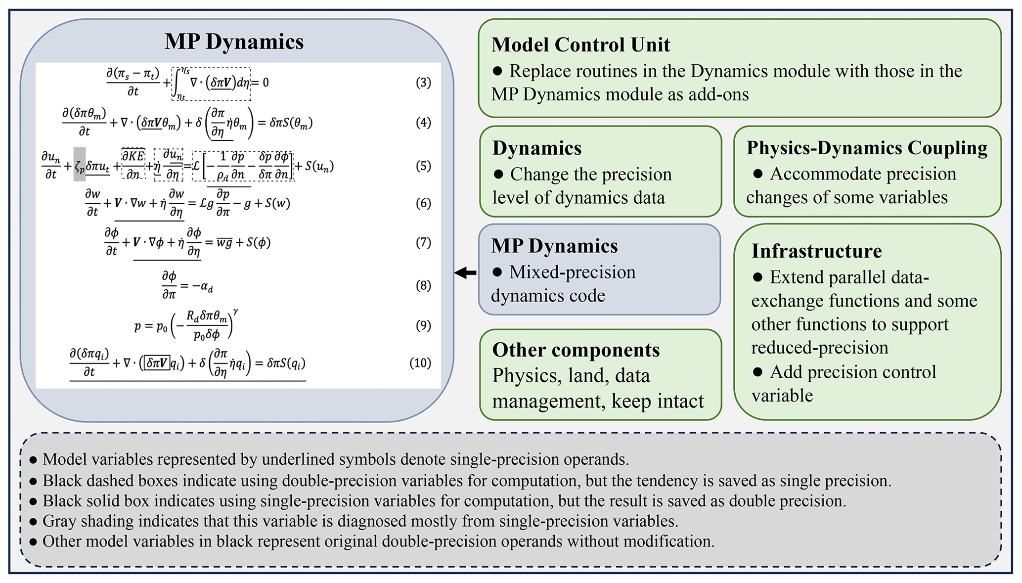
Figure 1Modifications to the GRIST model code repository for implementing the mixed-precision dynamical core.
1.2 Mixed-precision optimization strategy
The purpose of the mixed-precision optimization strategy is to decrease the precision level (and thus computational cost) while maintaining accuracy and stability. Before implementing mixed-precision computing, we checked that completely using single precision for the entire dynamical core leads to an unacceptable loss of accuracy (see Sect. 4.1). However, considering the extensive code base and its degree of complexity, comprehensively and randomly testing every component and variable is impractical. An iterative development approach with a minimum degree of trial and error is used to identify the model components that are sensitive to the precision level. The dry baroclinic wave of Jablonowski and Williamson (2006) is used as a benchmark test during the iterative development cycle because this case has complex fluid dynamics characteristics and is very sensitive to numerical precision.
We established an acceptable error threshold, α, to assess whether the difference between outcomes from double-precision and mixed-precision simulations falls within a tolerable limit. Results from the original double-precision computing serve as the true values. The iteration involves the execution of an initial 10 d simulation. We then embarked on a series of precision reduction tests for selected model variables, and we computed the error norm of selected diagnostic variables for each test. E is defined as representing the overall error level (calculated relative to the double-precision results):
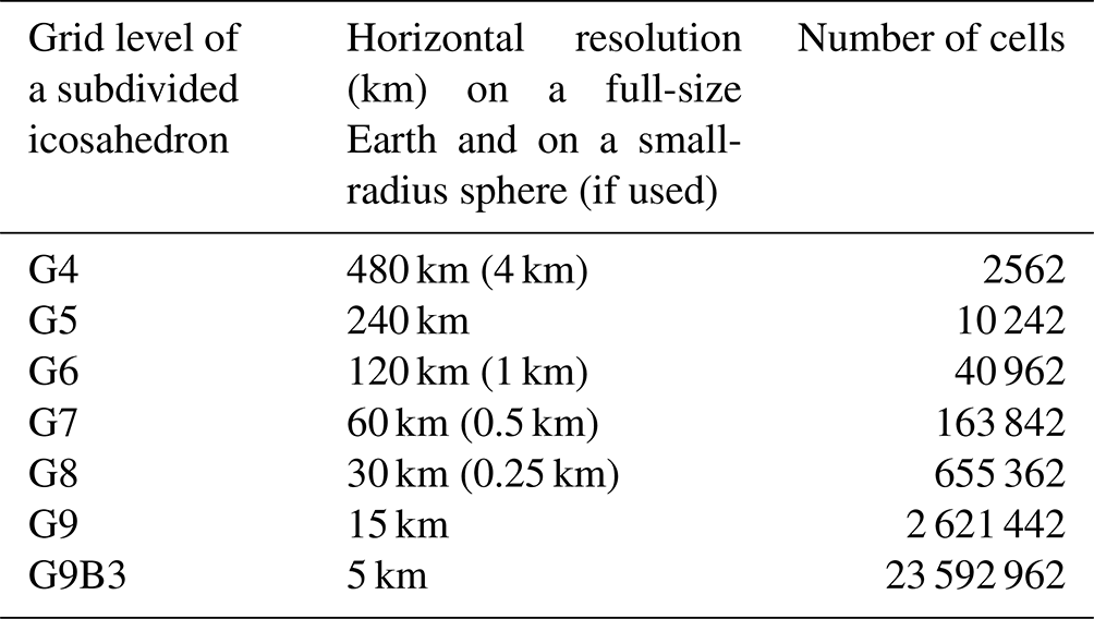
where L1, L2, and L∞ represent the first, second, and infinite norm of variable H, respectively. The definitions of L1, L2, and L∞ can be found in the Appendix. Should error E exceed α (0.05 for this study), the modification is deemed unacceptable and consequently abandoned; otherwise, the modification is accepted, allowing for a further reduction in variable precision based on this new configuration. This is an optimization approach similar to the greedy algorithm. Initially, by selecting single-precision variables, we systematically attempted to reduce the precision of variables encountered sequentially in the code, starting with the first variable, followed by the second, third, and so forth. The precision optimization tests were conducted using the G8 grid. The grid names and their corresponding resolutions are listed in Table 1. Initially, selected diagnostic variables (H) are ps (surface pressure) and vor (relative vorticity) because they can effectively quantify deviations in the mass field and velocity field. This criterion was set beforehand, but it has turned out that L(vor) has a much larger error magnitude than L(ps) overall. Thus, L(vor) determines our optimization outcome.
Technically, the switch between double-precision and single-precision code is defined through the Fortran KIND parameter, specified in a constant module. As single-precision results may not always replicate double-precision results and can occasionally generate unacceptable errors (e.g. see Sect. 3.2), it is crucial to identify precision-sensitive variables and solver components. An additional parameter “ns” has been introduced in this constant module for the precision-insensitive variables. This modification facilitates the transition between double-precision, single-precision, and mixed-precision computations. Note that only the subroutine of the solver is modified, indicating that the model initialization section remains in double-precision operations. If the solver requires single-precision operands, double-precision variables need to be converted to single precision after initialization. This method ensures a streamlined transition to mixed precision with minimal changes to the code structure.
Some important aspects are summarized as follows:
-
Model variables that are insensitive to the precision level are set to the ns parameter type. When ns is defined as single precision, the code executes mixed-precision computations; when defined as double precision, the code regresses double-precision computing and produces solutions that are identical to the original unmodified code.
-
We appropriately decompose computations involving implicit-type conversions to reduce performance degradation due to precision conversion. For instance, . Here, a is a single-precision floating point, b a larger double-precision float, and c a single-precision float. The conversion of c to double precision can introduce extra rounding errors. These errors, amplified by b, may accumulate over time, adversely affecting model outcomes. Single-precision calculations provide a consistent error boundary, unlike mixed precision which introduces uncertainty. In some cases, results might even be better if the computation of a function was entirely in single precision. Hence, optimization should proceed with caution, considering these error dynamics.
The Message Passing Interface (MPI) communication was modified for single-precision variables; the built-in functions, such as HUGE or TINY, are used to obtain very large or very small values, respectively, to ensure the values fall within the precision range of the variables.
1.3 Mixed-precision optimization results
Following the strategy outlined in Sect. 2.2, the mixed-precision GRIST dynamical core is established. The optimization results, as depicted on the left side of Fig. 1, are summarized based on the continuous-form governing equations. The meaning of each variable in the equations follows Zhang et al. (2020) exactly to avoid repeating explanations. Model variables with underlined text denote single-precision operands; variables in black represent double-precision operands. The black dashed boxes indicate that this part uses double-precision variables for computation, but the tendency is saved as single precision. The grey shading indicates that this variable is diagnosed mostly from single-precision variables. Specifically, is highly sensitive to the precision of δπ, requiring a double-precision δπ.
For the dycore, the precision sensitivity varies among different terms. The precision-sensitive terms are primarily related to pressure gradient and gravity terms. The precision-insensitive terms are mainly advective, which may tolerate lower numerical precision. Computationally, the advective parts of the equations use higher-order operators, which are responsible for the major computational burden. The passive tracer transport equation (Eq. 10) can mostly be computed using single precision. The only part that needs careful modification is the solid black box, which indicates that it uses single-precision variables for computing, but the result is saved as double precision. δπV (representing the mass flux) in Eq. (10) is accumulated and averaged from δπV in Eq. (3), so computing it uses single precision. But when using it for tracer transport, this variable is converted to double precision so that the mass continuity equation of tracer transport uses a double-precision mass flux.
The mass continuity equation (Eq. 3) is solved using a flux form, ensuring global mass conservation of πs−πt (πt is a constant) within the bounds of machine rounding errors, which is at the double-precision level. Using single-precision δπV implies that mass continuity is locally conserved at the single-precision level. Recognizing the potential importance of local mass conservation (e.g. Thuburn, 2008), a compilation switch is designed so that approximating δπV and the related mass continuity tendency can be achieved in either single precision or double precision. The time difference between approximating the continuity equation using single precision and double precision accounts for ∼1 %–2 % of the total computational time. We examine the model sensitivity to this operation in Sect. 4.4.
1.4 Model code modification
Figure 1 illustrates the modification made to the original model code repository. Thanks to the modular structure of the model code, the mixed-precision version of the model dynamics can be seamlessly integrated as an add-on component, allowing for independent development. The switch between double-precision and mixed-precision dynamics is governed by the model's control unit, facilitating the transition between two code repositories via a compiler option (MIXCODE). Additional adjustments for each component include modifying the parallel exchange functions to support reduced-precision variables, altering the precision level of allocated dynamics data, accommodating precision changes in specific variables in physics–dynamics coupling, and introducing a precision control variable. All these supplementary modifications are also designated by the compiler option MIXCODE. The pure single-precision code is achieved by simply using single precision for all variables, marked as SPCODE in the code. When MIXCODE is defined, additional variable allocations and assignment statements are introduced. It has been confirmed that overheads due to these additional statements can be omitted by comparing the original code to the MIX code executed in a pure double-precision mode.
We first examine the computational performance of the mixed-precision dynamical core in a standard reference computational test. Here, all computing tasks are carried out on a local supercomputing cluster. Each computing node is equipped with 128 GB memory, and the central processing unit (CPU) is a Hygon C86 7285 model at 2.0 GHz. Each CPU features a 32 KB L1 data cache, a 64 KB L1 instruction cache, a 512 KB L2 cache, and an 8192 KB L3 cache. We use SGL to denote pure single-precision computing, DBL to denote pure double-precision computing, and MIX to represent mixed-precision computing. All experiments were conducted on a G8 grid, submitted with the same topology: 756 MPI tasks distributed across six nodes.
Table 2Time elapsed using single, mixed, and double precision. (The runtime of each solver is normalized to that of the corresponding solver in double precision.)
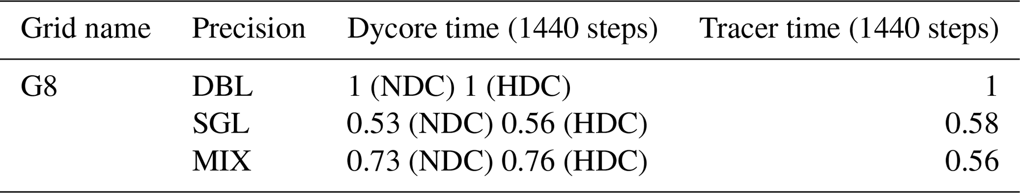
Compared to the double-precision model, the runtime of the mixed-precision model for the nonhydrostatic dry dynamical core (NDC), hydrostatic dry dynamical core (HDC), and tracer transport solver reduced by 27 %, 24 %, and 44 %, respectively (Table 2). The runtime of the mixed-precision dycore solver is still larger compared to the single-precision dycore, implying that there is time overhead incurred by the use of double precision in precision-sensitive algorithms. The runtime of the mixed-precision tracer transport solver is comparable to that of the single-precision tracer transport solver because most computations in the tracer transport module now use single-precision computing. It should be noted that the time gains from mixed-precision computing may also depend on hardware and compiler options (e.g. Brogi et al., 2024).
For real-world applications with routine I/O, the mixed-precision code maximizes its potential in global storm-resolving model (GSRM) simulations. In Sect. 4.5, the MIX run achieved a 25.5 % reduction in the wall-clock time for the dynamics and physics procedures (including physics–dynamics coupling), as compared with the DBL run. The simulations (5 km; 23 592 962 cells) were conducted using 3248 MPI processes distributed across 58 computing nodes, where each node is equipped with 56 Intel Xeon Gold 6348 CPUs operating at 2.60 GHz and 256 GB of memory. For both DBL and MIX runs, the dynamics and physics procedures (including physics–dynamics coupling) accounted for approximately 95 % of total wall-clock time, with dynamics alone occupying a substantial portion ranging from 83 % to 85 %.
For a computational task that is not significantly restricted by the memory bandwidth, the reduction in wall-clock time can be less significant. This is the case described in Sect. 4.4, in which a coarse-resolution (120 km; 40 962 cells) model is executed using 640 MPI processes across 20 nodes. The MIX test is faster than the DBL test by roughly 12 %.
As emphasized by one reviewer, reduced-precision computing can be particularly beneficial for the machines with sub-optimal interconnect, and on the graphic processing unit (GPU)-like architectures, where increased computational intensity (in terms of degrees of freedom per GPU) can increase the overall performance. Another application of this mixed-precision code also confirms this assertion. Thanks to Sunway's local engineers, this mixed-precision code has been successfully ported to the new Sunway supercomputer. Here, we report some observations; detailed results will be presented elsewhere.
One processor of Sunway has 390 cores, distributed across six core groups (CGs). Each CG consists of one management processing element (MPE) and 64 computing processing elements (CPEs) organized as an 8×8 array. Numerical tests were conducted at the 3.75 and 1.875 km (icosahedral grid levels 11 and 12) horizontal resolutions using the full model. A notable observation was that mixed precision typically did not yield significant speedup on the MPE side but provided notable speedup on the CPE-parallelized kernels. Considering that the Sunway architecture generally does not exhibit higher calculation performance for single precision compared to double precision (except for division and elemental functions), we may infer that the MPE-side code is not limited by the memory bandwidth. On CPEs, the mixed-precision code demonstrates better speedup. This implies that the performance of the CPE-side code is more constrained by the memory bandwidth, and thus mixed-precision computing leads to better improvements.
3.1 Moist baroclinic wave
To ensure robustness, a hierarchy of five test cases from simple to complex is adopted for model evaluation. This first case is from the DCMIP2016, as outlined by Ullrich et al. (2014), a modified approach to the dry baroclinic instability scenario (Jablonowski and Williamson, 2006). This experimental setup triggers the emergence of an unstable baroclinic wave pattern, initiated by early perturbations, which exhibits exponential growth and attains its maximum intensity around the 11th day. The experiment incorporates a passive tracer representing water vapour, which is subject to passive advection. Although the mixing ratio marginally influences the pressure gradient force, as noted by Zhang et al. (2020), the overall behaviour of wave growth is in substantial agreement with that in the dycore (Zhang et al., 2019). The primary objective is to assess the model's efficacy in replicating the typical dynamics of moist atmospheric conditions across various precision settings.
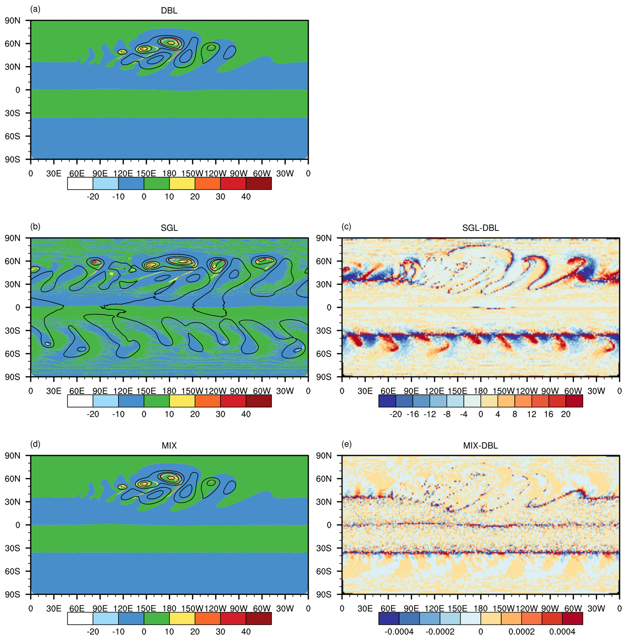
Figure 2Baroclinic wave development at day 11 in the (a) DBL simulation, (b) SGL simulation, and (d) MIX simulation. (a, b, d) The colours show relative vorticity ( s−1) and contours of the surface pressure and (c, e) the relative error between SGL and DBL, as well as the difference between MIX and DBL.
Figure 2 shows surface pressure and the relative vorticity field at the model level near 850 hPa (model layer 23, 30 layers in total) at day 11, as simulated by the G8 resolutions. The baroclinic waves show the anticipated growth in the DBL simulation (Fig. 2a). In the SGL simulation, the primary growth fluctuations in the DBL simulation were reproduced (Fig. 2c). However, in the Northern Hemisphere, there were developments of incorrect spurious waves, whose intensity was comparable to the major fluctuations (Fig. 2c). The Southern Hemisphere exhibited a weaker structure of spurious waves (Fig. 2c). The results from the MIX simulation displayed patterns much closer to those in the DBL simulation (Fig. 2e).
The primary difference between the MIX and DBL simulations lies in the vicinity of strong gradients along the cold front (Fig. 2c). But the primary fluctuations in both MIX and DBL simulations exhibit a high degree of similarity in their patterns (Fig. 2a and e), indicating that precision levels have a tangible impact on the phase speed of wave propagation.
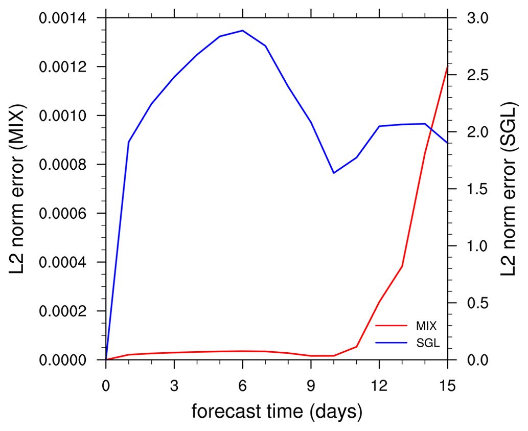
Figure 3Time evolution of the global l2 difference norm of simulated relative vorticity between the SGL and DBL and the l2 difference norm between the MIX and DBL. Red and blue represent SGL and MIX experiments, respectively.
The error introduced by SGL and MIX can be quantified by comparing their solutions to a DBL solution. Following Jablonowski and Williamson (2006), l2 error norms (defined in the Appendix) of the relativity vorticity field at the 23rd model layer are compared on the global grid as a function of time. Figure 3 shows the l2 norm for the SGL and MIX. In the initial stages of the model integration, the errors in the SGL simulations increased rapidly. By checking the original fields (figure not shown), it was found that numerous small-scale spurious fluctuations had emerged on both sides of the Equator, the intensity of which was similar to the physically meaningful fluctuations.
After day 6, the primary fluctuations in the baroclinic waves in the SGL simulations began to develop, resembling the behaviour of the DBL simulations, and the errors started to decrease (Fig. 3). By day 10, the fluctuations developed rapidly, the primary fluctuations grew robustly, and the spurious fluctuations produced in the early stages of the SGL simulations also developed rapidly, leading to an increase in errors (Fig. 3). On day 11, the intensity of the spurious fluctuations developed in SGL was close to that of the primary fluctuations, which is unacceptable. Due to the slow growth of the primary fluctuations in the early stages, the MIX simulation exhibited minimal errors before day 9 (Fig. 3). Subsequently, as the fluctuations matured rapidly, larger differences in the phase speed compared to the DBL emerged, leading to a rapid increase in errors.
3.2 Splitting supercell thunderstorms
The splitting supercell test of DCMIP2016 (Klemp et al., 2015; Zarzycki et al., 2019) emphasizes the importance of scrutinizing nonhydrostatic model simulations of small-scale dynamics, especially as models approach spatial resolutions on the (sub-)kilometre scale. This test utilized the small-planet testing framework (Wedi and Smolarkiewicz, 2009), a cost-effective approach by scaling down Earth's radius by a factor of 120. The model employs the Kessler warm-rain microphysics scheme for simplified physics. This particular test case is characterized by unstable atmospheric conditions conducive to moist convection, posing a challenge to numerical accuracy and stability. Klemp et al. (2015) suggested that an increase in horizontal resolution should lead to convergent solutions. For GRIST, this behaviour has been verified by Zhang et al. (2020). Our investigation further examines the capability of the MIX configuration to accurately replicate the behaviours observed in the DBL simulations.
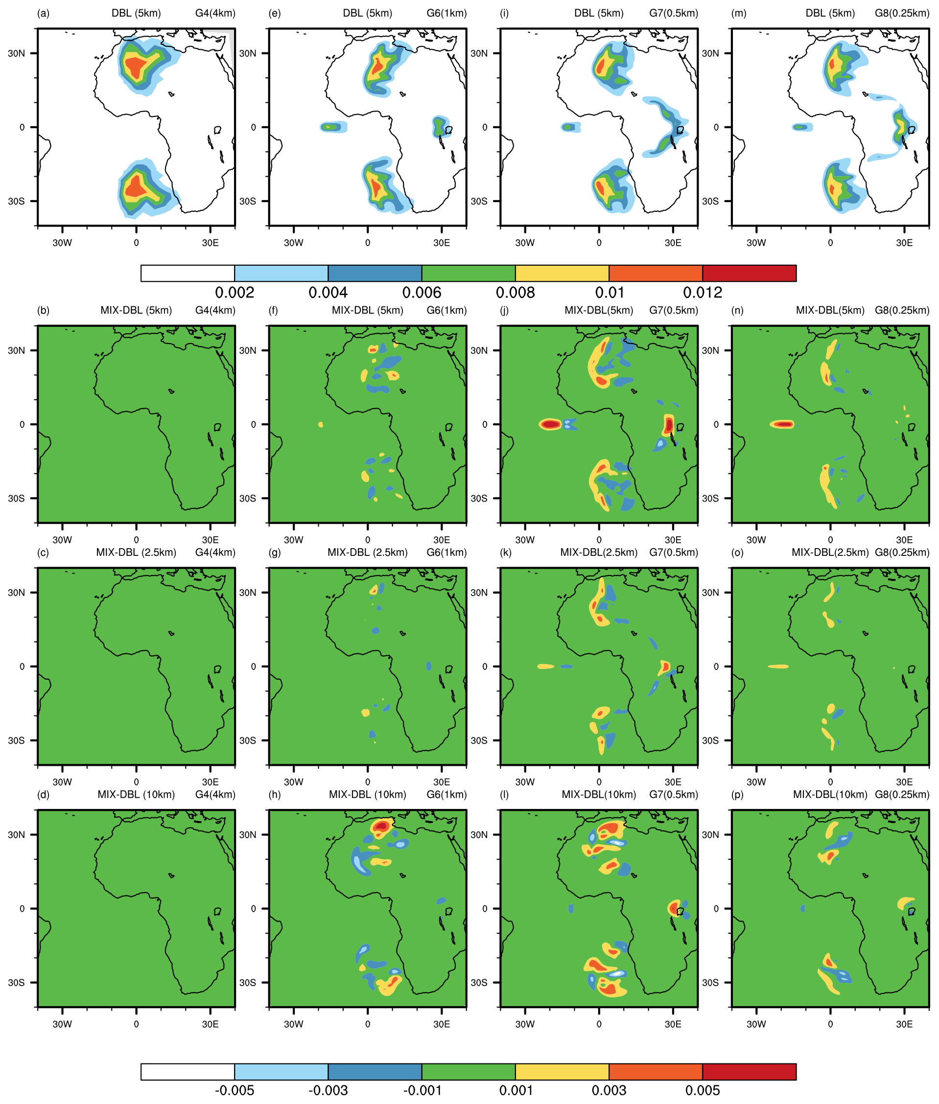
Figure 4Horizontal cross-sections of the rainwater mixing ratio at different heights from supercell thunderstorm simulations. The first row displays double-precision simulations at 5 km altitude. The second, third, and fourth rows show the differences between mixed-precision and double-precision simulations at 5, 2.5, and 10 km altitudes, respectively. The four columns represent results at different resolutions (from left to right): G4 (4 km), G6 (1 km), G7 (0.5 km), and G8 (0.25 km).
Figure 4 shows the qr mixing ratio at 5 km elevation in both DBL and MIX simulations at four resolution choices (G4: ∼4 km, G6: ∼1 km, G7: ∼0.5 km, and G8: ∼0.25 km). The DBL and MIX solutions show bulk similarities across all the resolutions. At 7200 s, a single updraught splits and evolves into a symmetric storm propagating towards the poles, with two supercells located ∼30° from the Equator. These supercells show subtle differences in their structure and intensity. At a low resolution of 4 km, the differences between the MIX and DBL simulations are minimal at all altitudes (Fig. 4b–c). As the resolution increases from 4 to 1 km and to 0.5 km, the structural differences in supercells gradually become more pronounced (Fig. 4b–d, f–h, j–l). However, when the resolution further increases from 0.5 to 0.25 km, the differences diminish (Fig. 4n–p). For DBL simulation results, the differences between 0.5 km and 0.25 km are smaller than those between 1 and 0.5 km, indicating that the solution converges at a resolution of almost 0.5 km. At 0.25 km, the results of the MIX simulation show greater similarity to those of the DBL simulation at all altitudes (Fig. 4n–p). This indicates that, in the mixed-precision simulation, supercells also achieved good convergence at this resolution, and thus the sensitivity to the precision level diminishes from 0.5 to 0.25 km.
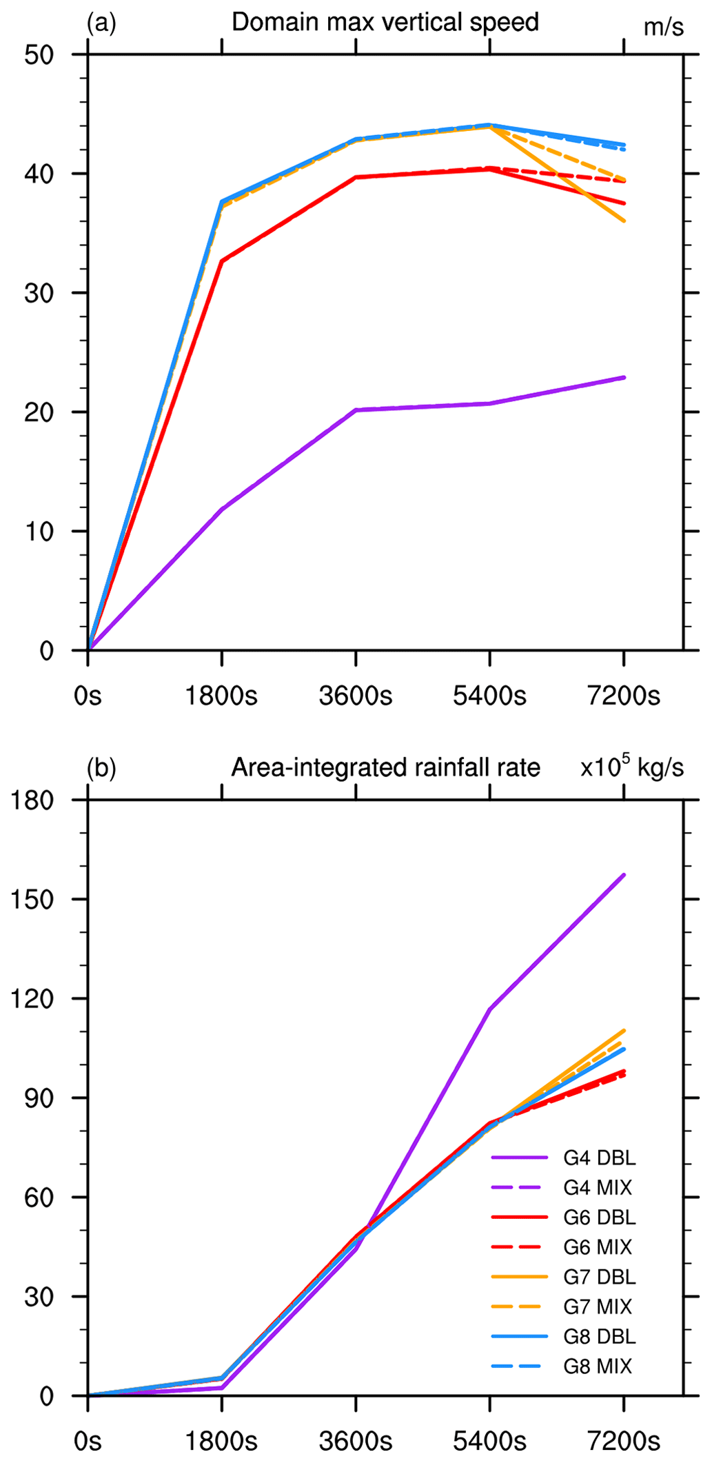
Figure 5The (a) domain maximum vertical speed and (b) area-integrated rainfall rate obtained from the supercell simulations.
Figure 5 shows the maximum vertical speed and area-integrated rainfall rate over the global domain as a function of time for each resolution. The vertical speed in both MIX and DBL increases with resolution (Fig. 5a). From the start of the model integration until 5400 s, the vertical speed curves of the MIX and DBL simulations nearly overlap (Fig. 5a). After 5400 s, a noticeable deviation appears, except for the G4 grid. The difference in vertical speed between MIX and DBL is minimal at 4 km resolution, followed by 0.25 km resolution, while it is larger at 1 and 0.5 km resolutions (Fig. 5a). The area-integrated rainfall rate curves exhibit similar evolutionary features (Fig. 5b). At very low resolutions, such as 4 km, the differences between the MIX and DBL simulations are not significant. At a higher resolution of 0.25 km, the overall behaviour of supercells in the MIX simulations is closer to that of DBL compared to 0.5 and 1 km resolutions. Both MIX and DBL solutions exhibit convergence behaviours.
3.3 Idealized tropical cyclone
This idealized tropical cyclone scenario integrates a three-dimensional dynamical core with a simple physics suite (Reed and Jablonowski, 2012), alongside an analytic vortex initialization technique (Reed and Jablonowski, 2011). The experiment produces the evolution of a tropical cyclone from a nascent, idealized vortex, highlighting the model's sensitivity to various parameter adjustments. Notably, alterations in the tracer transport schemes of GRIST can produce subtle sensitivities in the development of the tropical cyclone due to the pressure gradient terms (Zhang et al., 2020), thereby establishing this case as being useful for assessing model precision sensitivity.
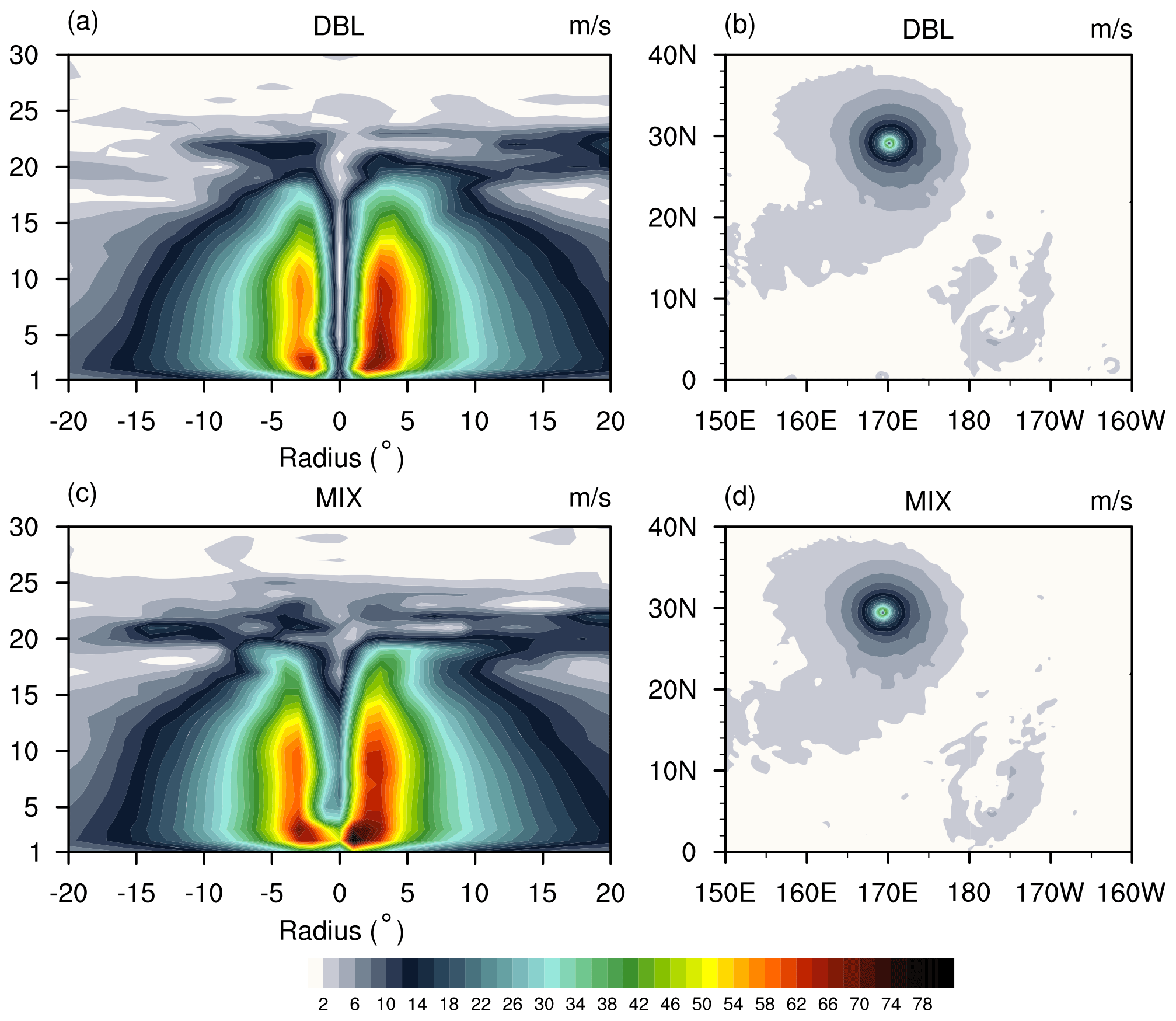
Figure 6The simulated wind speed (m s−1) at the G8 resolution with the NDC solver, including MIX (a, b) and DBL (c, d) simulations. (a, c) Longitude–height cross-section of the wind speed through the centre latitude of the vortex as a function of the radius from the vortex centre. (b, d) Horizontal cross-section of the wind speed at the lowest model layer.
Figure 6 displays the wind speed at day 10 for the DBL (Fig. 6a and b) and MIX (Fig. 6c and d) simulations at the G8 resolution. Figure 6 (left) shows the longitude–height cross-sections of the magnitude of the wind through the centre latitude of the vortex. Figure 6 (right) displays the horizontal cross-sections of the magnitude of the wind at the lowest model layer. The centre of the vortex is defined as the grid point with minimum surface pressure. At day 10, the developed storm resembled a tropical cyclone. The overall behaviour in the MIX simulation was similar to that in the DBL simulation, with maximum winds near the surface and a distinct eyewall structure (Fig. 6). However, there was some differences in the vertical structure and centre location of the cyclone (Fig. 6a and c). In the MIX simulation, the generated cyclone was stronger, with higher wind speeds near the surface (Fig. 6c). The eyewall of the cyclone in the MIX simulation appeared to be less pronounced compared to that in the DBL simulation, where the cyclone's eyewall was narrower and straighter (Fig. 6c). Overall, the characteristics of the cyclone were comparable between the MIX and DBL simulations.
In addition to two deterministic control simulations using both double precision and mixed precision with the nonhydrostatic solver, eight ensemble simulations are further performed with the double-precision nonhydrostatic model. This assesses the MIX simulation within the uncertainty range of the DBL simulation. The uncertainty range is quantified by the ensemble simulations encompassing eight initial-value perturbation members. Random small-amplitude perturbations were applied to the initial wind speeds (e.g. Li et al., 2020), where perturbations to the normal velocity at cell edges were prescribed within a range of 2 % of their values in the control experiment.
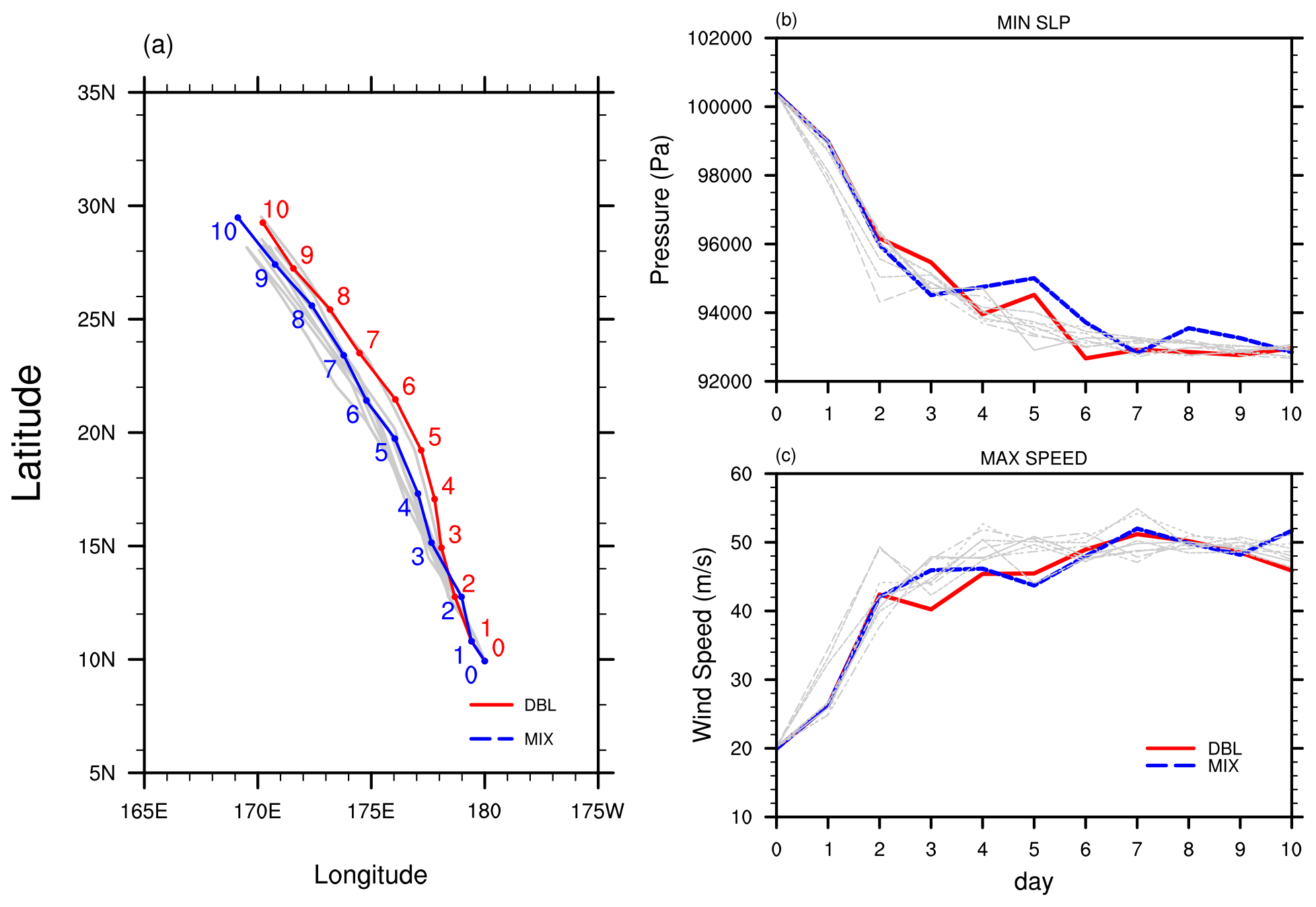
Figure 7The results from the deterministic and ensemble simulations. (a) The track of the tropical cyclone centre for the MIX (blue lines) and DBL (red lines) deterministic simulations. Time evolution of the (b) minimum surface pressure and (c) maximum surface wind speed from the deterministic and ensemble simulations. The red and blue lines represent the deterministic MIX and DBL simulations, respectively. The grey lines represent the eight runs with random perturbations to the initial normal velocity at the cell edges.
Figure 7 describes the tracks of tropical cyclones, along with the evolution of minimum surface pressure and maximum surface wind speed over time. The red and blue lines represent two deterministic simulations conducted using MIX and DBL solvers, respectively. The eight random perturbation simulations with the DBL solver are represented by grey lines. Minimal spread is observed in the early stages of the simulations (Fig. 7). Cyclone track separation between the MIX and DBL simulations occurs on day 1 (Fig. 7a). Subsequently, spread in the simulations increases over time (Fig. 7). The evolution of minimum surface pressure and maximum surface wind speed over time exhibits similar trends (Fig. 7b, c). No discernible difference is found between the sensitivity introduced by MIX and that introduced by perturbed DBL simulations. The overall behaviour of the MIX simulation falls within the range of uncertainty of the DBL simulation.
3.4 Atmospheric Model Intercomparison Project (AMIP) simulation
Following the establishment of the MIX dynamical core, a detailed examination of its integration with the model physics suite (Li et al., 2023) becomes crucial. The nonlinear interactions between the model's dynamics and its physical processes can result in varied performances across weather and climate simulations. It is imperative to investigate these differences to ensure that MIX simulations can accurately mirror the outcomes of DBL simulations in practical applications.
In assessing a new formulation for real-world modelling, our guiding principle is to first run long-term AMIP simulations (Zhang et al., 2021). This ensures that the model can achieve statistical equilibrium, maintain a realistic model climate, and have good integral properties such as conservation and balanced budgets (e.g. Fu et al., 2024). Subsequently, the same model, with minimal application-specific modifications, undergoes shorter-range but higher-resolution, kilometre-scale tests (Zhang et al., 2022).
The AMIP experiment is conducted in alignment with Zhang et al. (2021). This involved running both hydrostatic and nonhydrostatic models with the weather physics suite on a G6 grid over a decade, spanning 2001 to 2010. The simulations were performed under conditions with prescribed climatological sea surface temperatures and sea ice concentrations. The focus was narrowed to precipitation, which is a comprehensive metric due to its sensitivity to both model dynamics and physics, effectively reflecting the nonlinear interactions that are crucial for accurate weather and climate simulations (Zhang and Chen, 2016).
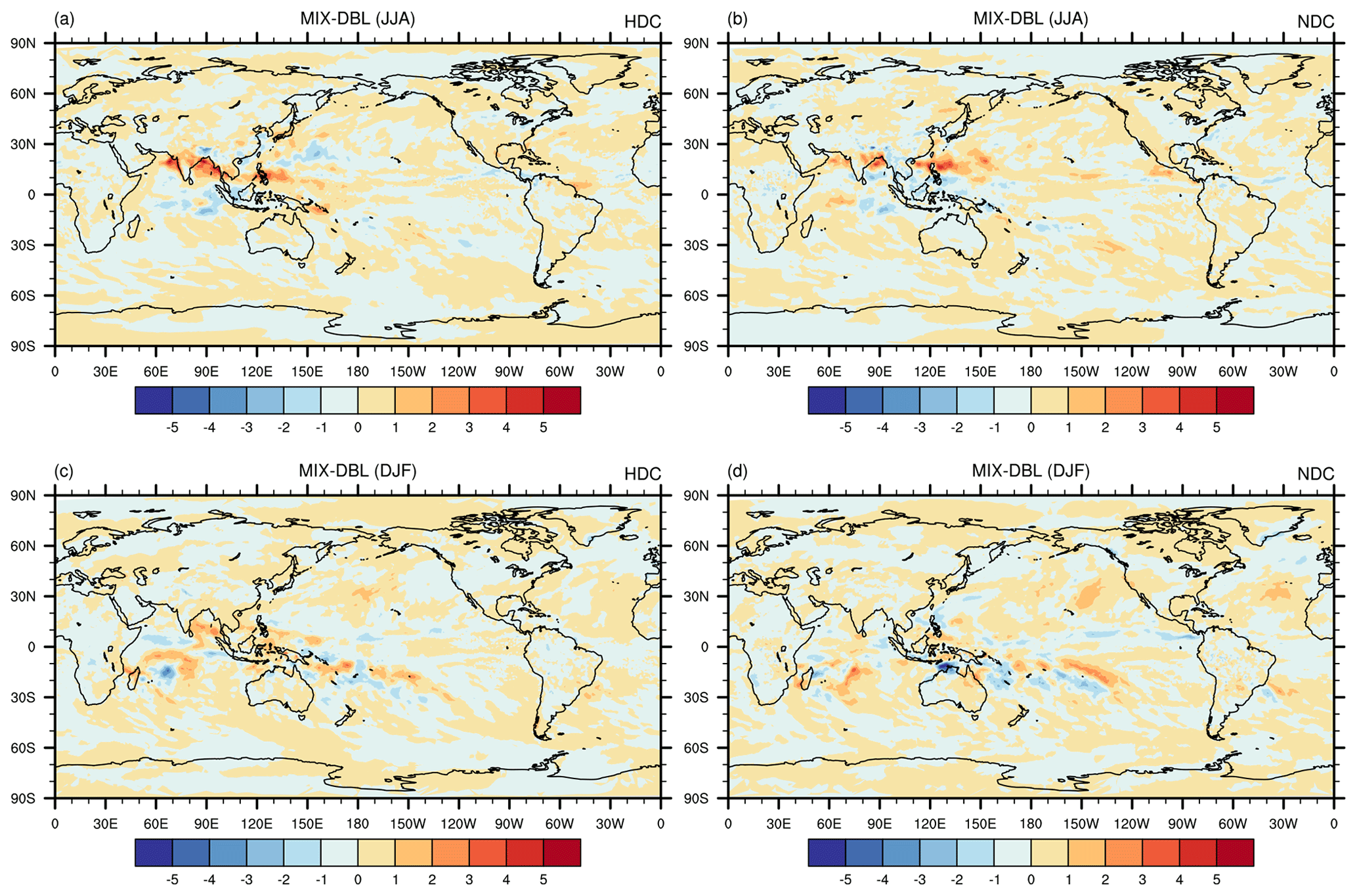
Figure 8The difference between the MIX and DBL simulations, including solutions from the hydrostatic (a, c) and nonhydrostatic (b, d) solvers. The first and second rows display the averaged (2001–2010) precipitation rate (mm d−1) for JJA and DJF, respectively.
Figure 8 shows the simulated climatological (2001–2010) precipitation field for June–July–August (JJA) and December–January–February (DJF). Both the hydrostatic and nonhydrostatic MIX solvers can replicate the JJA and DJF precipitation patterns in the DBL simulations. The discrepancies between the MIX and DBL simulations are similar in both hydrostatic and nonhydrostatic simulations, with the primary differences occurring in the tropics. The precipitation differences shift from north to south along with the main rain bands as the season transitions from (boreal) summer to winter. The deviation in summer precipitation is greater than that in winter precipitation because convective activities are most vigorous. In the summer, the MIX simulation overestimates the precipitation in the tropical coastal regions of the western Pacific, especially along the western coast (Fig. 8a and b). In winter, the main biases in the MIX simulation are concentrated in the Southern Ocean (Fig. 8c and d).
These results may have two implications. In MIX simulations, the cumulative effects of rounding errors might be progressively magnified over the course of long-term climate integrations. This phenomenon could lead to notable differences in the simulated large-scale atmospheric phenomena. This contrasts with high-resolution shorter-range weather modelling, where discrepancies primarily emerge at small scales, as is discussed in Sect. 4.5. This might imply that MIX simulations may diverge more from their DBL counterparts over extended integration periods, necessitating a careful consideration of how rounding errors accumulate and their impact on the climate simulation performance.
Second, the differences induced by varying the precision level can be further exacerbated by physical processes within the climate system. A clear example is observed in the tropical regions during the boreal summer, where higher discrepancies are noted. This suggests that certain atmospheric conditions or regions, such as the tropics during periods of intense solar heating, may be more susceptible to the effects of precision-level differences. These conditions can amplify the inherent precision differences, leading to more pronounced variations.
In the MIX implementation, Eq. (3) implies that global mass is conserved at the double-precision level. The local mass flux is only conserved at the single-precision level because the mass flux and its divergence are treated as single precision. As mentioned in Sect. 2.3, we retained the capability to compute the terms related to the mass flux divergence equation in the double precision as well. Local mass can be conserved at the double-precision level as well. We then evaluated the long-term climate integration results based on the hydrostatic model.
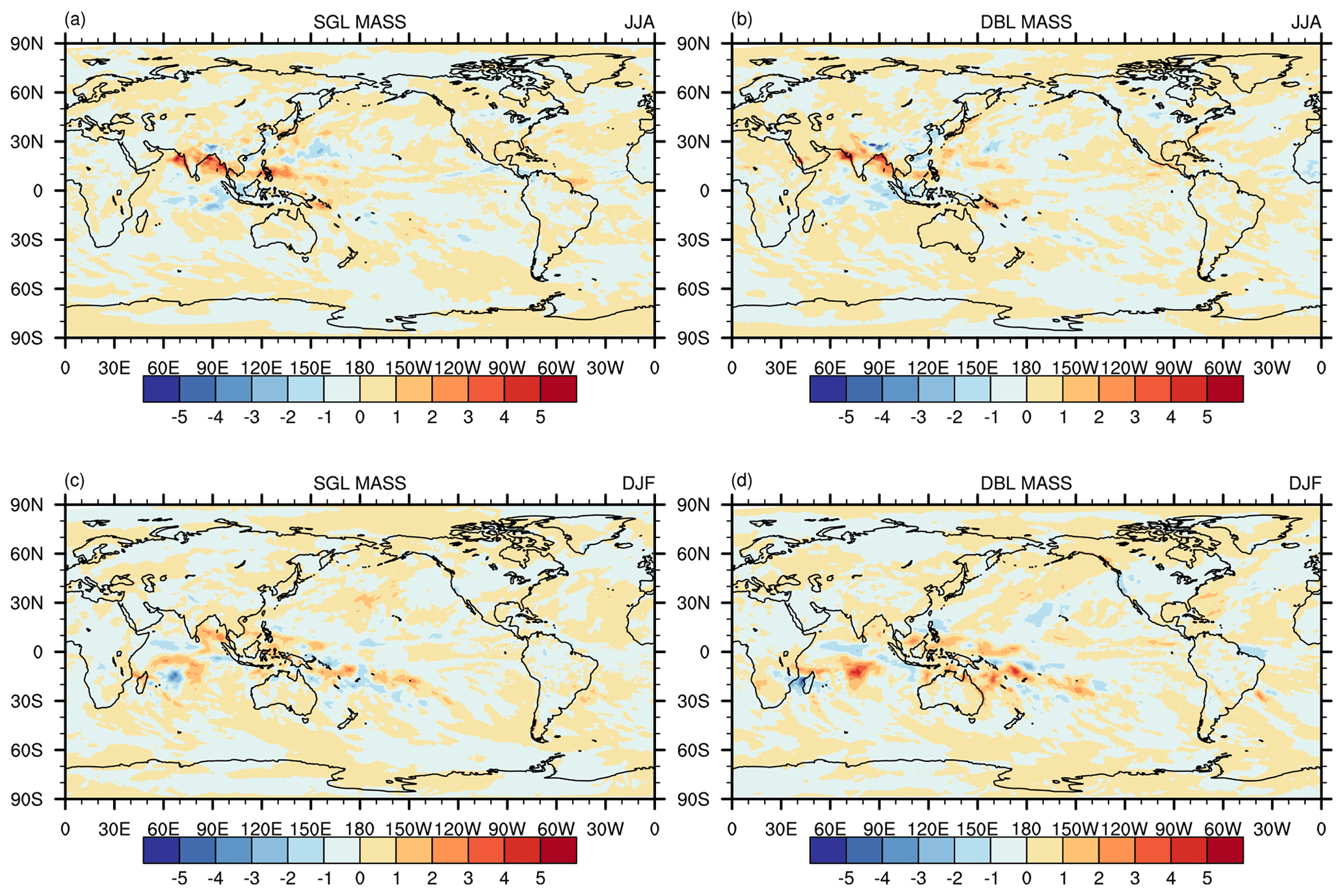
Figure 9(a) Difference between the JJA-averaged (2001–2010) precipitation rate (mm d−1) simulated by the SGL continuity equation solver in the mixed-precision mode and the “true DBL value”. (b) The same as (a) but for the DBL continuity equation solver. (c, d) The same as (a) (b) but for the DJF-averaged (2001–2010) results.
Figure 9 shows the differences in the climatological precipitation field between MIX with single- (MIX_SGL_mass) and double-precision (MIX_DBL_mass) mass flux divergence against the pure DBL simulation. In summer, the simulation differences between the MIX_SGL_mass and MIX_DBL_mass solvers are small (Fig. 9a and b). In winter, the deviations in the MIX_SGL_mass solver are smaller than those in the MIX_DBL_mass solver (Fig. 9c and d). The deviations are most pronounced in tropical convective precipitation over the southern tropical oceans (Fig. 9c and d). The larger difference between MIX_DBL_mass and DBL is likely due to implicit-type conversions, as discussed in Sect. 2.2.
3.5 A global storm-resolving simulation
Under the constraints of today's computational resources, executing GSRM nonhydrostatic simulations remains resource intensive (Satoh et al., 2017; Stevens et al., 2019). The use of MIX simulations presents a cost-effective solution to this challenge. However, it has been reported, for instance by Nakano et al. (2018), that as the resolution of the model increases, the difference between MIX and DBL may increase, especially for the smaller-scale flow features. This observation prompts a closer investigation into the performance of nonhydrostatic models at high-resolution modelling.
A GSRM experiment at 5 km (G9B3) is performed using the MIX nonhydrostatic model, following Zhang et al. (2022). The model was integrated from 00:00 UTC on 10 July to 00:00 UTC on 15 July 2015. We expect that the developed mixed-precision dynamical core can replicate the behaviour of DBL in the kilometre-scale weather simulations.
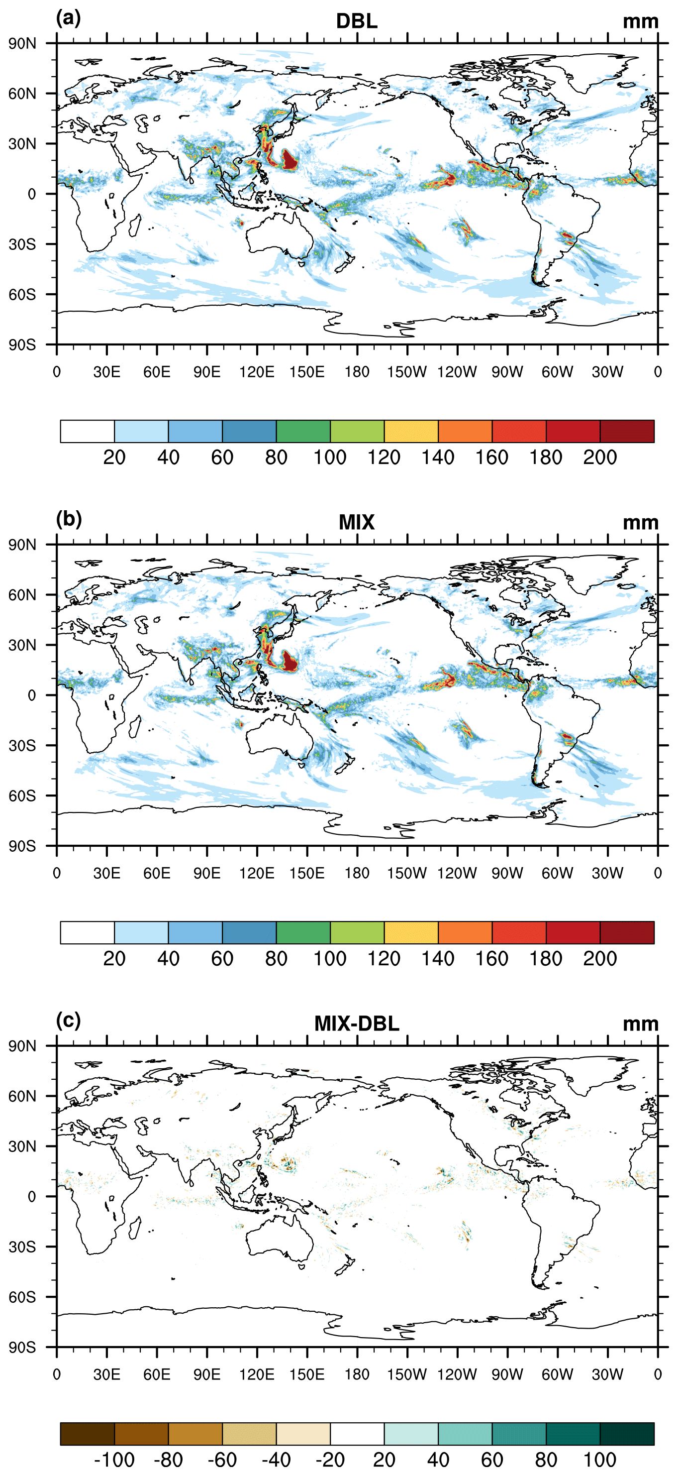
Figure 10The 5 d (00:00 UTC on 10 July to 00:00 UTC on 15 July 2015) accumulated precipitation (units: mm) from the (a) DBL simulation and (b) MIX simulation and (c) the difference between the MIX and DBL simulations.
Figure 10 shows the period-accumulated precipitation (00:00 UTC on 10 July to 00:00 UTC on 15 July) from the MIX and DBL model runs. All data have been interpolated onto a 0.5° regular latitude–longitude grid. The precipitation patterns simulated by MIX are very close to those of DBL simulations. MIX obtains nearly the same general position, orientation, and intensity of the rain band (Fig. 10a, b). MIX and DBL also produce very comparable kinetic energy spectra (figure not shown).
Like the AMIP simulations, the differences in precipitation are primarily located within the tropics, with the most pronounced differences in areas with vigorous convection. Close-ups of these locations reveal that it is small scales (a few grid spaces) that are most sensitive to the precision level because small scales are most sensitive to numerical discretization and dissipation (Jablonowski and Williamson, 2011). Considering that global mesoscale forecast at a few kilometres would greatly benefit from ensemble prediction (Palmer, 2019), in practice, the MIX-induced small-scale sensitivity may also fall within the uncertainty range of the ensemble, similar to that in Sect. 4.3.
As mentioned in Sect. 2.3, the advective parts of the equations are not sensitive to the precision level, and they use higher-order operators. To understand whether this optimization outcome is sensitive to the nominal order of numerics, we utilized an isolated three-dimensional tracer transport experiment (Kent et al., 2013; Hadley-like meridional circulation) and performed a convergence test. This test case was also performed by Zhang et al. (2020) and Li and Zhang (2022), and thus their results can be used as a reference. By adjusting the very small values introduced by the limiter to be within the single-precision range, this equation (Eq. 10 in Fig. 1) is solved independently in single precision (SPCODE compiler option in the model code).
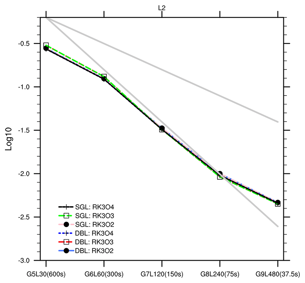
Figure 11The L2 norm error and convergence rate of the three-dimensional passive transport test (Hadley-like meridional circulation) using a single (SGL)-precision and double (DBL)-precision code for three horizontal flux operators: RK3O2, RK3O3, and RK3O4. The upper and lower grey lines correspond to the slopes of first- and second-order convergence rates, respectively.
We used various orders of horizontal flux operators, namely RK3O2, RK3O3, and RK3O4 (combinations of a third-order Runge–Kutta integration scheme and the nominal second- to fourth-order spatial flux operators). RK3O3 is used in other tests of this paper. The vertical advection operator remains unchanged. The results are shown in Fig. 11. The tested resolutions and associated time steps include G5L30 (600 s), G6L60 (300 s), G7L120 (150 s), G8L240 (75 s), and G9L480 (37.5 s). The results demonstrate that, using different-order horizontal flux operators, the single-precision simulations are comparable to the double-precision simulations across all resolutions, with nearly identical error norms and convergence rates.
This outcome suggests that, within the current code implementation, the advective part of the model demonstrates greater resilience when subjected to changes in precision, regardless of the nominal order of the numerical operator. This supports the optimization results in all dynamical equations. As reported by Nakano et al. (2018) and Yin et al. (2021), the precision-sensitive components are related to the specific numerical algorithms. Additionally, badly conditioned code or poor coding practice may also necessitate double-precision calculations (Váňa et al., 2016; Palmer, 2020). For other components (e.g. pressure gradient) that currently have higher sensitivity to the precision level, we believe that it may require more careful code implementation to allow us to benefit more from reduced-precision computing.
We consider this project to be a success, at least in its current phase. Existing literature and our own experiments suggest that the deviation between reduced-precision and double-precision codes tends to increase with higher resolutions. Therefore, the mixed-precision code optimization developed based on the G8 grid test can have relatively smaller deviations compared with the double-precision model on the coarser grids. While we cannot 100 % guarantee that the optimization outcome is optimal for all grid resolutions, the current 5 km test is also reasonable. Overall, we are confident that the present code will not degrade the operational skill score (e.g. those examined by Wang et al., 2024), but more testing efforts are still required for quality operational runs. In the future, we aim to further reduce the precision of certain variables and conduct more tests at the kilometre scale to ensure the robustness of the optimized code. Some alternative advection schemes in the tracer transport module have not been implemented in single precision yet, and this can be done in the future. Experiments with further reduced significant digits also deserve exploration.
In this study, we investigated mixed-precision computing within the GRIST dynamical core, identifying the equation terms that are particularly sensitive to numerical precision. We outlined an optimization procedure characterized by a limited extent of iterative development. Given the current development trajectory of high-performance computing, where advancements in memory bandwidth lag behind peak processor performance improvements, mixed-precision computation holds promise for enhancing weather and climate model development. The major conclusions are summarized as follows.
We discovered that terms sensitive to numerical precision primarily involve pressure gradient and gravity terms. In contrast, advective terms exhibit resilience to single precision and can be optimized. Advective terms are computationally more expensive than pressure gradient and gravity terms. The viability of employing mixed-precision computing in the GRIST dynamical core has been validated across a spectrum of scenarios, from idealized flow to real-world AMIP and GSRM simulations. These MIX experiments yielded results remarkably similar to those from the DBL simulations. For dycore, the runtime for the dry hydrostatic and dry nonhydrostatic cores was reduced by 24 % and 27 %, respectively. The tracer transport module witnessed a runtime reduction of 44 %. The overall time savings depend on the proportion of dycore and tracer transport in the total wall-clock time, as well as the scale of a computational task, which varies by application. For instance, the MIX-GSRM experiment in Sect. 4.5 witnessed a 25.5 % reduction in the wall-clock time compared with the DBL-GSRM experiment.
We noted a higher sensitivity to precision in long-term climate simulations compared to short-term higher-resolution weather simulations, particularly affecting the precipitation field over certain regions. In shorter-range weather forecast, the differences between MIX and DBL are mainly found at small scales, while in the AMIP simulations, the difference is found at larger scales. These effects may primarily stem from the model sensitivity to the precision level or from biases introduced by mixed-precision computations themselves. Compared with the low-resolution global simulations, the mixed-precision code is more beneficial for the GSRM simulations at a scale of a few kilometres or other model applications with computational scales comparable to GSRMs.
We define the three-dimensional global integral of H as
where A denotes the cell area, and z denotes height. The vertical integral is omitted if two-dimensional space is under consideration. The definitions of L1, L2, and L∞ are as follows:
where H and HT are the computational solution and true solution, respectively, and means selecting the maximum value from the field.
Model code and plotting data related to this paper are available at https://doi.org/10.5281/zenodo.11229770 (GRIST-Dev, 2024).
SC developed the mixed-precision model code and prepared the initial draft. YZ designed and led this model development research. YW contributed to experiments. All authors discussed this work and contributed to the final version of the paper.
The contact author has declared that none of the authors has any competing interests.
Publisher's note: Copernicus Publications remains neutral with regard to jurisdictional claims made in the text, published maps, institutional affiliations, or any other geographical representation in this paper. While Copernicus Publications makes every effort to include appropriate place names, the final responsibility lies with the authors.
The editors and reviewers are thanked for their handling of and comments on this paper.
This research has been supported by the National Youth Talent Project (grant no. 2021).
This paper was edited by Peter Caldwell and reviewed by Filip Vana and Luca Bertagna.
Abdelfattah, A., Anzt, H., Boman, E. G., Carson, E., Cojean, T., Dongarra, J., Fox, A., Gates, M., Higham, N. J., Li, X. S., Loe, J., Luszczek, P., Pranesh, S., Rajamanickam, S., Ribizel, T., Smith, B. F., Swirydowicz, K., Thomas, S., Tomov, S., Tsai, Y. M., and Yang, U. M.: A survey of numerical linear algebra methods utilizing mixed-precision arithmetic, The Int. J. High Perform. C., 35, 344–369, https://doi.org/10.1177/10943420211003313, 2021.
Baboulin, M., Buttari, A., Dongarra, J., Kurzak, J., Langou, J., Langou, J., Luszczek, P., and Tomov, S.: Accelerating scientific computations with mixed precision algorithms, Comput. Phys. Commun., 180, 2526–2533, https://doi.org/10.1016/j.cpc.2008.11.005, 2009.
Banderier, H., Zeman, C., Leutwyler, D., Rüdisühli, S., and Schär, C.: Reduced floating-point precision in regional climate simulations: an ensemble-based statistical verification, Geosci. Model Dev., 17, 5573–5586, https://doi.org/10.5194/gmd-17-5573-2024, 2024.
Bauer, P., Dueben, P. D., Hoefler, T., Quintino, T., Schulthess, T. C., and Wedi, N. P.: The digital revolution of Earth-system science, Nat. Comput. Sci., 1, 104–113, https://doi.org/10.1038/s43588-021-00023-0, 2021.
Benjamin, S. G., Brown, J. M., Brunet, G., Lynch, P., Saito, K., and Schlatter, T. W.: 100 Years of Progress in Forecasting and NWP Applications, Meteorol. Monogr., 59, 13.11–13.67, https://doi.org/10.1175/AMSMONOGRAPHS-D-18-0020.1, 2019.
Brogi, F., Bnà, S., Boga, G., Amati, G., Esposti Ongaro, T., and Cerminara, M.: On floating point precision in computational fluid dynamics using OpenFOAM, Future Gener. Comp. Sy., 152, 1–16, https://doi.org/10.1016/j.future.2023.10.006, 2024.
Chantry, M., Thornes, T., Palmer, T., and Düben, P.: Scale-Selective Precision for Weather and Climate Forecasting, Mon. Weather Rev., 147, 645–655, https://doi.org/10.1175/MWR-D-18-0308.1, 2019.
Cotronei, A. and Slawig, T.: Single-precision arithmetic in ECHAM radiation reduces runtime and energy consumption, Geosci. Model Dev., 13, 2783–2804, https://doi.org/10.5194/gmd-13-2783-2020, 2020.
Düben, P. D. and Palmer, T. N.: Benchmark Tests for Numerical Weather Forecasts on Inexact Hardware, Mon. Weather Rev., 142, 3809–3829, https://doi.org/10.1175/MWR-D-14-00110.1, 2014.
Düben, P. D., McNamara, H., and Palmer, T. N.: The use of imprecise processing to improve accuracy in weather & climate prediction, J. Comput. Phys., 271, 2–18, https://doi.org/10.1016/j.jcp.2013.10.042, 2014.
Düben, P. D., Russell, F. P., Niu, X., Luk, W., and Palmer, T. N.: On the use of programmable hardware and reduced numerical precision in earth-system modeling, J. Adv. Model. Earth Sy., 7, 1393–1408, https://doi.org/10.1002/2015MS000494, 2015.
Fornaciari, W., Agosta, G., Cattaneo, D., Denisov, L., Galimberti, A., Magnani, G., and Zoni, D.: Hardware and Software Support for Mixed Precision Computing: a Roadmap for Embedded and HPC Systems, 2023 Design, Automation & Test in Europe Conference & Exhibition (DATE), 1–6, 2023.
Fu, H., Liao, J., Ding, N., Duan, X., Gan, L., Liang, Y., Wang, X., Yang, J., Zheng, Y., Liu, W., Wang, L., and Yang, G.: Redesigning CAM-SE for peta-scale climate modeling performance and ultra-high resolution on Sunway TaihuLight, Proceedings of the International Conference for High Performance Computing, Networking, Storage and Analysis, Denver, Colorado, 2017.
Fu, Z., Zhang, Y., Li, X., and Rong, X.: Intercomparison of Two Model Climates Simulated by a Unified Weather-Climate Model System (GRIST), Part I: Mean State, Clim. Dynam., https://doi.org/10.1007/s00382-024-07205-2, 2024.
Gan, L., Fu, H., Luk, W., Yang, C., Xue, W., Huang, X., Zhang, Y., and Yang, G.: Accelerating solvers for global atmospheric equations through mixed-precision data flow engine, 2013 23rd International Conference on Field programmable Logic and Applications, 2–4 September 2013, Porto, Portugal, 1–6, 2013.
GRIST-Dev: Mixed-Precision Computing in the GRIST Dynamical Core for Weather and Climate Modeling, Zenodo [code and data], https://doi.org/10.5281/zenodo.11229770, 2024.
Gu, J., Feng, J., Hao, X., Fang, T., Zhao, C., An, H., Chen, J., Xu, M., Li, J., Han, W., Yang, C., Li, F., and Chen, D.: Establishing a non-hydrostatic global atmospheric modeling system at 3-km horizontal resolution with aerosol feedbacks on the Sunway supercomputer of China, Sci. B., 67, 1170–1181, https://doi.org/10.1016/j.scib.2022.03.009, 2022.
Harris, L. M. and Lin, S.-J.: A Two-Way Nested Global-Regional Dynamical Core on the Cubed-Sphere Grid, Mon. Weather Rev., 141, 283–306, https://doi.org/10.1175/MWR-D-11-00201.1, 2012.
Jablonowski, C. and Williamson, D. L.: A baroclinic instability test case for atmospheric model dynamical cores, Q. J. Roy. Meteor. Soc., 132, 2943–2975, https://doi.org/10.1256/qj.06.12, 2006.
Jablonowski, C. and Williamson, D.: The Pros and Cons of Diffusion, Filters and Fixers in Atmospheric General Circulation Models, in: Lauritzen, P. H., Jablonowski, C., Taylor, M. A., and Nair, R. D., Numerical Techniques for Global Atmospheric Models, Lecture Notes in Computational Science and Engineering, Springer, 80, 381–493, 2011.
Kent, J., Ullrich, P. A., and Jablonowski, C.: Dynamical core model intercomparison project: Tracer transport test cases, Q. J. Roy. Meteor. Soc., 140, 1279–1293, https://doi.org/10.1002/qj.2208, 2013.
Klemp, J. B., Skamarock, W. C., and Park, S. H.: Idealized global nonhydrostatic atmospheric test cases on a reduced-radius sphere, J. Adv. Model. Earth Sy., 7, 1155–1177, https://doi.org/10.1002/2015MS000435, 2015.
Li, J. and Zhang, Y.: Enhancing the stability of a global model by using an adaptively implicit vertical moist transport scheme, Meteorol. Atmos. Phys., 134, 55, https://doi.org/10.1007/s00703-022-00895-5, 2022.
Li, X., Peng, X., and Zhang, Y.: Investigation of the effect of the time step on the physics–dynamics interaction in CAM5 using an idealized tropical cyclone experiment, Clim. Dynam., 55, 665–680, https://doi.org/10.1007/s00382-020-05284-5, 2020.
Li, X., Zhang, Y., Peng, X., Zhou, B., Li, J., and Wang, Y.: Intercomparison of the weather and climate physics suites of a unified forecast–climate model system (GRIST-A22.7.28) based on single-column modeling, Geosci. Model Dev., 16, 2975–2993, https://doi.org/10.5194/gmd-16-2975-2023, 2023.
Maynard, C. M. and Walters, D. N.: Mixed-precision arithmetic in the ENDGame dynamical core of the Unified Model, a numerical weather prediction and climate model code, Comput. Phys. Commun., 244, 69–75, https://doi.org/10.1016/j.cpc.2019.07.002, 2019.
Nakano, M., Yashiro, H., Kodama, C., and Tomita, H.: Single Precision in the Dynamical Core of a Nonhydrostatic Global Atmospheric Model: Evaluation Using a Baroclinic Wave Test Case, Mon. Weather Rev., 146, 409–416, https://doi.org/10.1175/MWR-D-17-0257.1, 2018.
Palmer, T.: The ECMWF ensemble prediction system: Looking back (more than) 25 years and projecting forward 25 years, Q. J. Roy. Meteor. Soc., 145, 12–24, https://doi.org/10.1002/qj.3383, 2019.
Palmer, T. N.: The physics of numerical analysis: a climate modelling case study, Philos. T. Roy. Soc. A, 378, 20190058, https://doi.org/10.1098/rsta.2019.0058, 2020.
Reed, K. A. and Jablonowski, C.: An Analytic Vortex Initialization Technique for Idealized Tropical Cyclone Studies in AGCMs, Mon. Weather Rev., 139, 689–710, https://doi.org/10.1175/2010mwr3488.1, 2011.
Reed, K. A. and Jablonowski, C.: Idealized tropical cyclone simulations of intermediate complexity: A test case for AGCMs, J. Adv. Model. Earth Sy., 4, M04001, https://doi.org/10.1029/2011MS000099, 2012.
Santos, F. F. D., Carro, L., Vella, F., and Rech, P.: Assessing the Impact of Compiler Optimizations on GPUs Reliability, ACM Trans. Archit. Code Optim., 21, 26, https://doi.org/10.1145/3638249, 2024.
Satoh, M., Tomita, H., Yashiro, H., Kajikawa, Y., Miyamoto, Y., Yamaura, T., Miyakawa, T., Nakano, M., Kodama, C., Noda, A. T., Nasuno, T., Yamada, Y., and Fukutomi, Y.: Outcomes and challenges of global high-resolution non-hydrostatic atmospheric simulations using the K computer, Prog. Earth Planet. Sci., 4, 13, https://doi.org/10.1186/s40645-017-0127-8, 2017.
Sergeev, D. E., Mayne, N. J., Bendall, T., Boutle, I. A., Brown, A., Kavčič, I., Kent, J., Kohary, K., Manners, J., Melvin, T., Olivier, E., Ragta, L. K., Shipway, B., Wakelin, J., Wood, N., and Zerroukat, M.: Simulations of idealised 3D atmospheric flows on terrestrial planets using LFRic-Atmosphere, Geosci. Model Dev., 16, 5601–5626, https://doi.org/10.5194/gmd-16-5601-2023, 2023.
Skamarock, W. C., Klemp, J. B., Duda, M. G., Fowler, L. D., Park, S.-H., and Ringler, T. D.: A Multiscale Nonhydrostatic Atmospheric Model Using Centroidal Voronoi Tesselations and C-Grid Staggering, Mon. Weather Rev., 140, 3090–3105, https://doi.org/10.1175/MWR-D-11-00215.1, 2012.
Stevens, B., Satoh, M., Auger, L., Biercamp, J., Bretherton, C. S., Chen, X., Düben, P., Judt, F., Khairoutdinov, M., Klocke, D., Kodama, C., Kornblueh, L., Lin, S.-J., Neumann, P., Putman, W. M., Röber, N., Shibuya, R., Vanniere, B., Vidale, P. L., Wedi, N., and Zhou, L.: DYAMOND: the DYnamics of the Atmospheric general circulation Modeled On Non-hydrostatic Domains, Prog. Earth Planet. Sci., 6, 61, https://doi.org/10.1186/s40645-019-0304-z, 2019.
Taylor, M., Caldwell, P. M., Bertagna, L., Clevenger, C., Donahue, A., Foucar, J., Guba, O., Hillman, B., Keen, N., Krishna, J., Norman, M., Sreepathi, S., Terai, C., White, J. B., Salinger, A. G., McCoy, R. B., Leung, L.-y. R., Bader, D. C., and Wu, D.: The Simple Cloud-Resolving E3SM Atmosphere Model Running on the Frontier Exascale System, Proceedings of the International Conference for High Performance Computing, Networking, Storage and Analysis, 29 August 2023, Denver, CO, USA, 2023.
Thornes, T., Düben, P., and Palmer, T.: On the use of scale-dependent precision in Earth System modelling, Q. J. Roy. Meteor. Soc., 143, 897–908, https://doi.org/10.1002/qj.2974, 2017.
Thuburn, J.: Some conservation issues for the dynamical cores of NWP and climate models, J. Comput. Phys., 227, 3715–3730, https://doi.org/10.1016/j.jcp.2006.08.016, 2008.
Tomita, H. and Satoh, M.: A new dynamical framework of nonhydrostatic global model using the icosahedral grid, Fluid Dynam. Res., 34, 357, https://doi.org/10.1016/j.fluiddyn.2004.03.003, 2004.
Ullrich, P. A., Melvin, T., Jablonowski, C., and Staniforth, A.: A proposed baroclinic wave test case for deep- and shallow-atmosphere dynamical cores, Q. J. Roy. Meteor. Soc., 140, 1590–1602, https://doi.org/10.1002/qj.2241, 2014.
Váňa, F., Düben, P., Lang, S., Palmer, T., Leutbecher, M., Salmond, D., and Carver, G.: Single Precision in Weather Forecasting Models: An Evaluation with the IFS, Mon. Weather Rev., 145, 495–502, https://doi.org/10.1175/MWR-D-16-0228.1, 2016.
Wang, Y., Li, X., Zhang, Y., Yuan, W., Zhou, Y., and Li, J.: Performance analysis of Precipitation Forecast by the baseline version of GRIST Global 0.125-degree weather model configuration, Chinese Journal of Atmospheric Sciences, https://doi.org/10.3878/j.issn.1006-9895.2309.22223, 2024 (in Chinese with English Abstract).
Wedi, N. P. and Smolarkiewicz, P. K.: A framework for testing global non-hydrostatic models, Q. J. Roy. Meteor. Soc., 135, 469–484, https://doi.org/10.1002/qj.377, 2009.
Wedi, N. P., Polichtchouk, I., Dueben, P., Anantharaj, V. G., Bauer, P., Boussetta, S., Browne, P., Deconinck, W., Gaudin, W., Hadade, I., Hatfield, S., Iffrig, O., Lopez, P., Maciel, P., Mueller, A., Saarinen, S., Sandu, I., Quintino, T., and Vitart, F.: A Baseline for Global Weather and Climate Simulations at 1 km Resolution, J. Adv. Model. Earth Sy., 12, e2020MS002192, https://doi.org/10.1029/2020MS002192, 2020.
Yang, C., Xue, W., Fu, H., You, H., Wang, X., Ao, Y., Liu, F., Gan, L., Xu, P., Wang, L., Yang, G., and Zheng, W.: 10M-Core Scalable Fully-Implicit Solver for Nonhydrostatic Atmospheric Dynamics, SC '16: Proceedings of the International Conference for High Performance Computing, Networking, Storage and Analysis, 13–18 November 2016, Utah, Salt Lake City, 57–68, 2016.
Yin, F., Song, J., Wu, J., and Zhang, W.: An implementation of single-precision fast spherical harmonic transform in Yin–He global spectral model, Q. J. Roy. Meteor. Soc., 147, 2323–2334, https://doi.org/10.1002/qj.4026, 2021.
Yu, R., Zhang, Y., Wang, J., Li, J., Chen, H., Gong, J., and Chen, J.: Recent Progress in Numerical Atmospheric Modeling in China, Adv. Atmos. Sci., 36, 938–960, https://doi.org/10.1007/s00376-019-8203-1, 2019.
Zängl, G., Reinert, D., Rípodas, P., and Baldauf, M.: The ICON (ICOsahedral Non-hydrostatic) modelling framework of DWD and MPI-M: Description of the non-hydrostatic dynamical core, Q. J. Roy. Meteor. Soc., 141, 563–579, https://doi.org/10.1002/qj.2378, 2015.
Zarzycki, C. M., Jablonowski, C., Kent, J., Lauritzen, P. H., Nair, R., Reed, K. A., Ullrich, P. A., Hall, D. M., Taylor, M. A., Dazlich, D., Heikes, R., Konor, C., Randall, D., Chen, X., Harris, L., Giorgetta, M., Reinert, D., Kühnlein, C., Walko, R., Lee, V., Qaddouri, A., Tanguay, M., Miura, H., Ohno, T., Yoshida, R., Park, S.-H., Klemp, J. B., and Skamarock, W. C.: DCMIP2016: the splitting supercell test case, Geosci. Model Dev., 12, 879–892, https://doi.org/10.5194/gmd-12-879-2019, 2019.
Zhang, Y.: Extending High-Order Flux Operators on Spherical Icosahedral Grids and Their Applications in the Framework of a Shallow Water Model, J. Adv. Model. Earth Sy., 10, 145–164, https://doi.org/10.1002/2017MS001088, 2018.
Zhang, Y. and Chen, H.: Comparing CAM5 and Superparameterized CAM5 Simulations of Summer Precipitation Characteristics over Continental East Asia: Mean State, Frequency–Intensity Relationship, Diurnal Cycle, and Influencing Factors, J. Climate, 29, 1067–1089, https://doi.org/10.1175/JCLI-D-15-0342.1, 2016.
Zhang, Y., Li, J., Yu, R., Zhang, S., Liu, Z., Huang, J., and Zhou, Y.: A Layer-Averaged Nonhydrostatic Dynamical Framework on an Unstructured Mesh for Global and Regional Atmospheric Modeling: Model Description, Baseline Evaluation, and Sensitivity Exploration, J. Adv. Model. Earth Sy., 11, 1685–1714, https://doi.org/10.1029/2018MS001539, 2019.
Zhang, Y., Li, J., Yu, R., Liu, Z., Zhou, Y., Li, X., and Huang, X.: A Multiscale Dynamical Model in a Dry-Mass Coordinate for Weather and Climate Modeling: Moist Dynamics and Its Coupling to Physics, Mon. Weather Rev., 148, 2671–2699, https://doi.org/10.1175/MWR-D-19-0305.1, 2020.
Zhang, Y., Yu, R., Li, J., Li, X., Rong, X., Peng, X., and Zhou, Y.: AMIP Simulations of a Global Model for Unified Weather-Climate Forecast: Understanding Precipitation Characteristics and Sensitivity Over East Asia, J. Adv. Model. Earth Sy., 13, e2021MS002592, https://doi.org/10.1029/2021MS002592, 2021.
Zhang, Y., Li, X., Liu, Z., Rong, X., Li, J., Zhou, Y., and Chen, S.: Resolution Sensitivity of the GRIST Nonhydrostatic Model From 120 to 5 km (3.75 km) During the DYAMOND Winter, Earth Space Sci., 9, e2022EA002401, https://doi.org/10.1029/2022EA002401, 2022.
Zhang, Y., Li, J., Zhang, H., Li, X., Dong, L., Rong, X., Zhao, C., Peng, X., and Wang, Y.: History and Status of Atmospheric Dynamical Core Model Development in China, in: Numerical Weather Prediction: East Asian Perspectives, edited by: Park, S. K., Springer International Publishing, Cham, 3–36, 2023.