ShellSet v1.1.0 parallel dynamic neotectonic modelling: a case study using Earth5-049

We present a parallel combination of existing, well-known and robust software used in modelling the neotectonics of planetary lithosphere, which we call ShellSet. An added parallel framework allows multiple models to be run at the same time with varied input parameters. Additionally, we have included a grid search option to automatically generate models within a given parameter space. ShellSet offers significant advantages over the original programs through its simplicity, efficiency and speed. We demonstrate the performance improvement obtained by ShellSet's parallel framework by presenting timing and speedup information for a parallel grid search, varying the number of processes and models, on both a typical computer and a high-performance computing cluster node. A possible use case for ShellSet is shown using two examples in which we improve on an existing global model. In the first example we improve the model using the same data, and in the second example we further improve the model through the addition of a new scoring dataset. The necessary ShellSet program version along with all the required input and post-processing files needed to recreate the results presented in this article are available at https://doi.org/10.5281/zenodo.7986808 (May et al., 2023).

1 Introduction

Recent decades have seen significant progress made in the numerical modelling of lithospheric and crustal-scale processes. Simulations have become increasingly complex, and it often remains difficult to determine the best set of model parameters for a specific simulation, especially if non-linear rheologies or 3D effects are involved. Currently, the determination of the best set of model parameters is usually done by iteratively changing the model input parameters, performing numerous simulations, and scoring them against a particular class of observations, e.g. GPS measurements, stress tensor orientations or earthquake production rates.

There has been a significant improvement in computational power, efficiency and machine availability since the first computers were utilised for scientific purposes. Research institutions, both academic and industrial (public and private), provide employees with personal machines for their work. Even the least powerful of these machines is typically capable of simulations, serially and in parallel, that would have required much more expensive hardware only a decade previously. This allows many more simulations to be performed within any given period and larger models to be tested, which means that scientific knowledge is being improved almost by the second. In short, present-day scientists have access to more computing power than ever.

Unfortunately, this rapid improvement in computing power has, in some cases, outstripped the ability of widely used and scientifically robust programs to efficiently use the hardware available. For example, the programs Plasti, Ellipsis3D and ConMan – see Fuller et al. (2006), Moresi et al. (2007) and King et al. (2020) – all remain serial. Others, e.g. SNAC and Gale (Choi et al., 2008; Moresi et al., 2012), solve models in parallel using the Message Passing Interface (MPI) to distribute the work across multiple cores; however, they solve one model at a time, requiring the user to update input parameters between queued models or to launch multiple models in parallel manually. Whilst this parallelisation of the program will yield a performance benefit, should a user wish to perform multiple models, a manual procedure is not the most efficient one – especially if a methodological set of models is required, e.g. when searching for an optimal value within a particular parameter or set of parameters.

Shells is another program which, while it can solve a single model in parallel, requires a set of models to be controlled manually. Shells is a dynamic neotectonic modelling program first developed and released in 1995 (Kong and Bird, 1995). Since then it has had several updates, the most recent one being released in 2019. Shells uses the Intel Math Kernel Library (MKL) to solve systems of linear equations in parallel, which means that, unlike the previously noted parallel software which uses the MPI, Shells uses OpenMP style threads to parallelise its model. This limits the number of tasks possible in parallel as these threads are limited to a single shared-memory compute device, whereas the MPI can span a distributed memory machine. Due to this, Shells is unable to fully utilise the currently available computing hardware and is also unable to automatically search for an optimal value or set of values for input parameter(s).

In this work, we present ShellSet, which is composed of (i) OrbData5, a program used to alter the input finite-element grid (FEG) file, which we will refer to as OrbData; (ii) Shells, a dynamic neotectonic modelling program using finite elements; and (iii) OrbScore2, a scoring program which we will refer to as OrbScore. A brief explanation of the functionality of each can be found in Sect. 2.1, 2.2 and 2.3, respectively. Both OrbData and OrbScore function in conjunction with Shells by design. The input FEG file can be created using a separate program (OrbWin) maintained by, and available from, the author of Shells, OrbData and OrbScore.

Our program is based entirely on freely distributed software, with OrbData, Shells and OrbScore all being available at http://peterbird.name/index.htm (last access: 1 May 2024). All program dependencies, i.e. the Intel Fortran compiler, Intel MKL and MPI environment, are available from Intel within the base and high-performance computing (HPC) oneAPI toolkits. The final program runs in a Linux operating system (OS) environment using either a guest Linux OS on Windows machines (e.g. WSL2) or directly on Linux OS machines, including HPC structures. It requires Python3 for the use of its (optional) graphical user interface (GUI) and scatter plotter routines.

This work serves as an introduction to the neotectonic modelling community of ShellSet, an MPI parallel combination of existing, well-known, robust and widely used software. The version of ShellSet used for this article, along with all the input files, examples and user documentation, is available online: see https://doi.org/10.5281/zenodo.7986808 (May et al., 2023). In the following work we will use the term “model” to refer to a single model (defined by its input parameters), while “test” refers to a set of models.

2 Software

At the base of ShellSet are three existing programs: OrbData, Shells and OrbScore. Despite recent updates, these three programs remain both serial and separate by design. This requires the user to manually control all the files required by each program, which may be complicated further depending on the settings for Shells simulations. For example, previously generated output is often required to be read before the next Shells solution iteration begins. We outline the function of each of these programs in the following sections.

2.1 OrbData

Before deformation of the lithosphere can be modelled, its present structure must be defined, including its surface elevations, layer (crust and mantle-lithosphere) thicknesses, densities and parameters, which define its internal temperatures. These quantities must be specified for each node in the finite-element grid, which defines the domain of the model. OrbData calculates this lithosphere structure, which is used as an input to both Shells and OrbScore, using simple local operations on published datasets, often in spatially gridded formats. OrbData does not affect the topology of the finite-element grid or its included fault network.

OrbData computes the crustal and mantle-lithosphere thicknesses based on assumptions of local isostasy and either (a) a steady-state geotherm or (b) seismically determined layer thicknesses. It incorporates seismic constraints by adding two adjustable parameters, the density anomaly of the lithosphere of compositional origin and an extra quadratic curvature of the geotherm due to transient cooling or heating. These extra values are then incorporated into the finite-element grid at each node. For a description of the various algorithms OrbData uses, see Bird et al. (2008).

Whether the finite-element grid needs updating by OrbData depends on which input variables have been altered. We therefore consider OrbData to be optional – it is strictly required in some cases but is unnecessary in others. ShellSet takes this consideration away from the user by automatically deciding whether or not a certain parameter change requires an update to the finite-element grid. This decision is hard-coded into the program and is based on which input parameters are altered within a test.

Table 1 List of the misfit scoring options available in ShellSet.

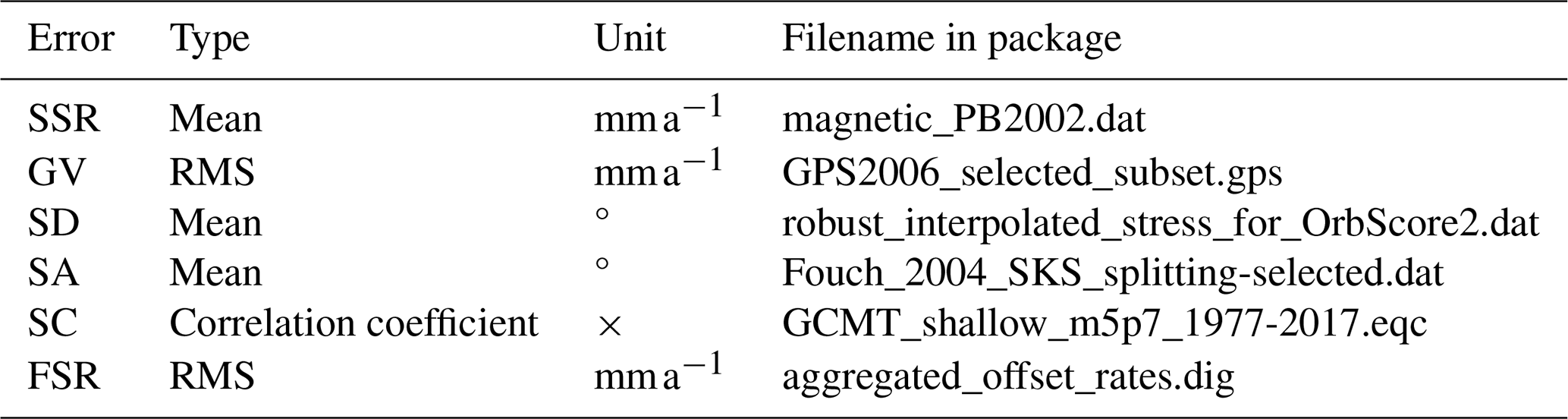
SSR – seafloor spreading rate. GV – geodetic velocity. SD – most-compressive horizontal stress direction. SA – fast-polarisation azimuths of split SKS waves. SC – smoothed seismicity correlation. FSR – fault slip rates. SSR, GV, SD, SA and FSR are misfits. SC is a score. The type of score reported for each error can be changed by altering a single line of the OrbScore source code within ShellSet.
× This error type is unit-less.

2.2 Shells

Shells is the leading program for those who want to conduct physics-based simulations of planetary tectonics with the efficiency of 2D spherical FE grids. Most competing programs use 3D grids, e.g. Ellipsis3D, SNAC, CitComCU and CitComS (Moresi et al., 2007; Choi et al., 2008; Moresi et al., 2009, 2014), while Gale (Moresi et al., 2012) has 2D and 3D functionalities. The 3D grids will typically require greater computing resources for comparable domain sizes (depending on the mesh size), and therefore they limit the number of experiments that are practical in parallel.

Shells uses the thermal and compositional structures of thin spherical shells (usually called “plates”) of the planetary lithosphere, together with the physics of quasi-static creeping flow, to predict patterns of velocity, straining and fault slip on the surface of a planet. Since the first publications outlining the first release version, Kong and Bird (1995) and Bird (1998), Shells has been updated and used in numerous publications, including Liu and Bird (2002a), Liu and Bird (2002b), Bird et al. (2006), Bird et al. (2008), Kalbas et al. (2008), Stamps et al. (2010), Jian-jian et al. (2010), Austermann et al. (2011), Carafa et al. (2015) and more recently Tunini et al. (2017). A primary goal is to understand the balance of the forces that move the plates, while a secondary goal is to predict fault slip rates and distributed strain rates for seismic hazard estimation.

Shells is serial in its application, except in two parts of its calculations, where it makes use of the thread-safe Intel MKL routines dgbsv and dgesv. These routines apply OpenMP-type threading within their execution if the problem size is large enough. The number of parallel threads used within each MKL routine is decided at runtime by the routines, although it will default to the number of physical cores, and environment variables can be altered to specify a strict number or to allow a dynamic selection of threads for MKL routines.

Shells produces six testable predicted fields in each model: relative velocities of geodetic benchmarks, most-compressive horizontal principal stress azimuths, long-term fault heave and throw rates, rates of seafloor spreading, distribution of seismicity on the map as well as fast-polarisation directions of split SKS arrivals. Each of these predictions can be scored against observed data.

Shells contains the possibility of defining lateral variations in lithospheric rheology within the model by updating the FEG file using an additional numerical ID for groups of elements. This ID number should correspond to a value within a separate file which defines the values of the four input parameters which describe frictional rheology at low temperatures, including an option for lower effective friction in fault elements. Nine describe the dislocation–creep flow laws of the crust and mantle-lithosphere layers of the lithosphere. All elements placed within one of these groups will take their values from this new file; only elements within the default group (ID = 0) will take values from the standard parameter input file.

2.3 OrbScore

OrbScore is used to score any of the six testable Shells predictions, for relative realism, against supplied real data. These six options are seafloor spreading rates (SSRs), geodetic velocities (GVs), most-compressive horizontal principal stress directions (SDs), fast-polarisation azimuths of split SKS waves (SA), smoothed seismicity correlation (SC) and fault slip rates (FSRs). Information on the SSR, GV, SD and SA datasets can be found in Sect. 6.1, 6.2, 6.3 and 6.4, respectively, of Bird et al. (2008). The FSR dataset was developed recently, and information on the dataset generation can be seen in Appendix A. The SC scoring dataset (not used in this work) is taken from the global centroid–moment–tensor (GCMT) catalogue. The basic methodology and approach used in that project are outlined in Dziewonski et al. (1981), with the most recent description of the analyses, including some significant improvements, given in Ekström et al. (2012).

Table 1 lists the six misfit scoring options along with the type of error reported, their units and the name of the file containing the dataset provided within the ShellSet package. Using one score or a combination of these calculated misfit scores, it is possible to compare different models and perform tuning of the input parameters to obtain the best misfit score for a particular scoring setup. The best misfit score then provides the optimal values for the tested variables.

In this work, as in Bird et al. (2008), we use a geometric mean of misfits to grade each model. The geometric mean is defined as the nth root of the product of n (assumed positive) numbers:

$$\begin{array}{}\text{(1)}& \mathrm{GM}=\sqrt[n]{S_{\mathrm{1}}{S}_{\mathrm{2}}\mathrm{\dots }{S}_n}.\end{array}$$

This is preferable to any arithmetic mean because the ranking of models using the geometric mean is independent of the units of the ingredient misfits.

3 ShellSet

Since the three individual programs are quick in their current form and are intrinsically linked in their work, we focused in this work on combining them into a single entity. Previously, in order to perform multiple models in parallel, the user would have to start multiple models in separate instances and control each one individually. In ShellSet the program controls the runs for each, running several in parallel if the compute resources exist. This simplifies the user interface while simultaneously leveraging parallel computing to obtain multiple results at the same time. This streamlined process has multiple benefits for the user and their work when compared with the three underlying programs. We will now outline some of the most important additions to the program and state the improvements that these have yielded, which ShellSet offers over the original separate programs.

3.1 Grid search

We have programmed two options for the alteration of multiple variables in parallel: a list input and a grid search. Each of these options requires one simple input file to be completed which defines the variables being tested, together with their values, or ranges, for the list input or grid search, respectively. While other parameter space sampling methods exist (see Reuber, 2021, for an analysis of the various options), we chose to add a grid search as it is simple to program and understand while offering consistent information across the entire parameter space. This means that, should only a simple visualisation of the misfit scores over a parameter space be required, a single-level grid search would provide total coverage with consistent spacing, while a random search, for example, would not necessarily provide consistent detail over the entire space.

A grid search is a searching algorithm used to tune parameters towards optimal values within a defined N-dimensional parameter space. Several different schemes can be used in a grid search for how the domain is divided, how to pass the best models to the next level, etc. However, we use the most basic version. This works by partitioning the parameter space into a grid of equal N-dimensional cells. Each cell is represented by a single central model whose location defines the value for each of the tested parameters. The upper-left image of Fig. 1 shows an initial 2 × 2 grid in a 2D space, with each of the four models represented by a coloured point.

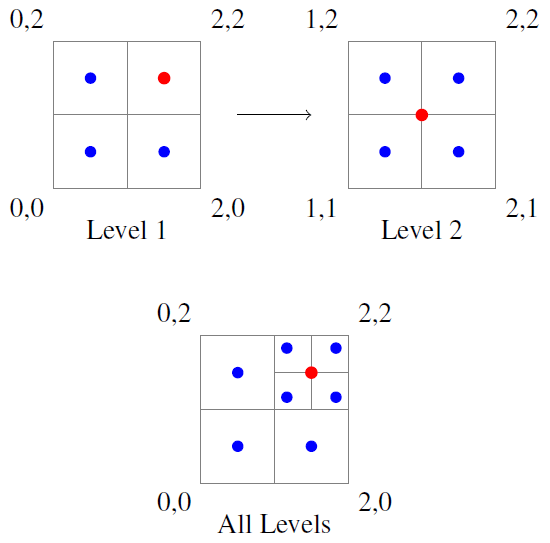
Figure 1 Example two-level grid search that selects a best cell (red point) and divides that cell into four new cells.

After a full grid of models has been simulated, the algorithm will select a defined number of best models to continue on to the next level. Each of the selected models has its cell divided in the same fashion as the first level (to scale) and representative models at the centre of each cell. In this way the algorithm progressively reduces the size of the searched parameter space by reducing the sizes of the cells, dividing increasingly smaller parameter spaces into cells, and selecting from their best models for further analysis. A typical algorithm will continue in this way until a defined stopping criterion is met, e.g. a specified number of levels, a desired model score or a total number of models.

Figure 1 shows the transition from a single best model to a new level. The red point in the upper-left image represents the best model, which is selected for the next level shown in the upper-right image. The lower image of Fig. 1 shows an overview of these two levels.

The base grid search algorithm was adapted from the Fortran grid search version available from May (2022). Like the original, the grid search used in ShellSet has no limit on the number of dimensions it is possible to use.

In ShellSet we rank the models using their misfit scores before selecting the best models and refining the search area within the parameter space. Since each model, at each level, is independent, an automated search of the parameter space may be performed by the program in parallel (see Sect. 3.2). This parallel search of the parameter space finds optimal values for desired variables quickly and efficiently (see Sect. 5) and allows the program to search each individual parameter to degrees of accuracy that are useful to the user but ordinarily tedious to perform manually.

ShellSet's grid search will work to a defined number of levels, whereupon the program will stop. It also optionally allows the user to define a target misfit score. When any model reaches or surpasses this value, the program will stop on completion of that level.

The inclusion of a search algorithm necessitated an additional set of checks to be performed on combinations of input parameters. Originally the programs performed only basic checks (unrealistic value entries on individual parameters, etc.) as a human user was assumed to be in control of all the input values. The grid search option essentially replaces the human user with a machine user, which theoretically allows for unrealistic selections of values for input variables. For example, in a test including both fault friction and continuum friction, the fault friction must be less than the continuum friction. This is something which a user would ordinarily handle manually, but the grid search algorithm must be controlled using additional checks to prevent unrealistic models from being performed. New checks are added to a separated source code file to simplify future updates. We currently place only the most general conditions on some variables (fault friction must be less than continuum friction and the mean mantle density must be greater than that of the crust), and any user is advised to add any necessary conditions to this file, depending on their local or global model requirements, in order to keep these conditions in a single location.

3.2 ShellSet parallelism

The grid search algorithm is made considerably more efficient if multiple models at the same level are run in parallel. For example, looking at Fig. 1, we can see that at the first level there are four distinct models which could all be performed in parallel, and at the second level there are another four. Knowing this, we have placed ShellSet in a simple MPI framework which allows the running of multiple models in parallel.

Using the MPI to perform multiple models in parallel, ShellSet also maintains the parallelism inherent in the Intel MKLs. Therefore, each model run by an MPI process is able to leverage a team of MKL threads within its call to the dgbsv and dgesv routines if there are available computing resources.

By default, the Intel MKL routines will set the number of threads to a value based on the problem size and the number of available cores at runtime. This behaviour can be problematic when running multiple models in parallel using the MPI, and although it can be changed by altering the program source code (requiring compilation to take effect), we have added a simple control on the maximum number of threads which may be used by MKL routines. The results shown in Sect. 5.1 demonstrate why allowing the MKL routines to select the number of threads automatically is not always optimal – particularly when the possibility of running multiple models in parallel exists. ShellSet calculates the number of free cores available per MPI process at runtime and sets the maximum number of threads available to MKL routines to this value. This calculation does not require any extra information from the user.

The migration of file control to the program was necessary to run multiple models in parallel without constant user input. This is discussed in more detail in Sect. 3.3.

3.3 User interface

As noted previously, some design features which were necessary in order to perform multiple models in parallel have also caused some unintended usability improvements. These, along with designed usability improvements present at its interface with the user, will be discussed now in terms of both input to the program and output from it.

The main output of ShellSet is a single file which defines the command line arguments used to start the program, along with a list of results in which a row represents a model. For every model the altered variables (those defined in the grid search or list input files) are recorded, along with all the calculated misfit results, a global model ID number and the ID of the MPI process which performed the model. The two ID numbers allow the user to trace the OrbData, Shells and OrbScore output files related to that model for further analysis. While this output file was not necessary when manually controlling a set of models, its addition in ShellSet gives an immediate general understanding of the test results while reporting information required to conduct a deeper examination of the selected models. This is possible as all output files from OrbData, Shells and OrbScore are saved in private directories with locations and filenames containing the process ID, model number and Shells iteration number.

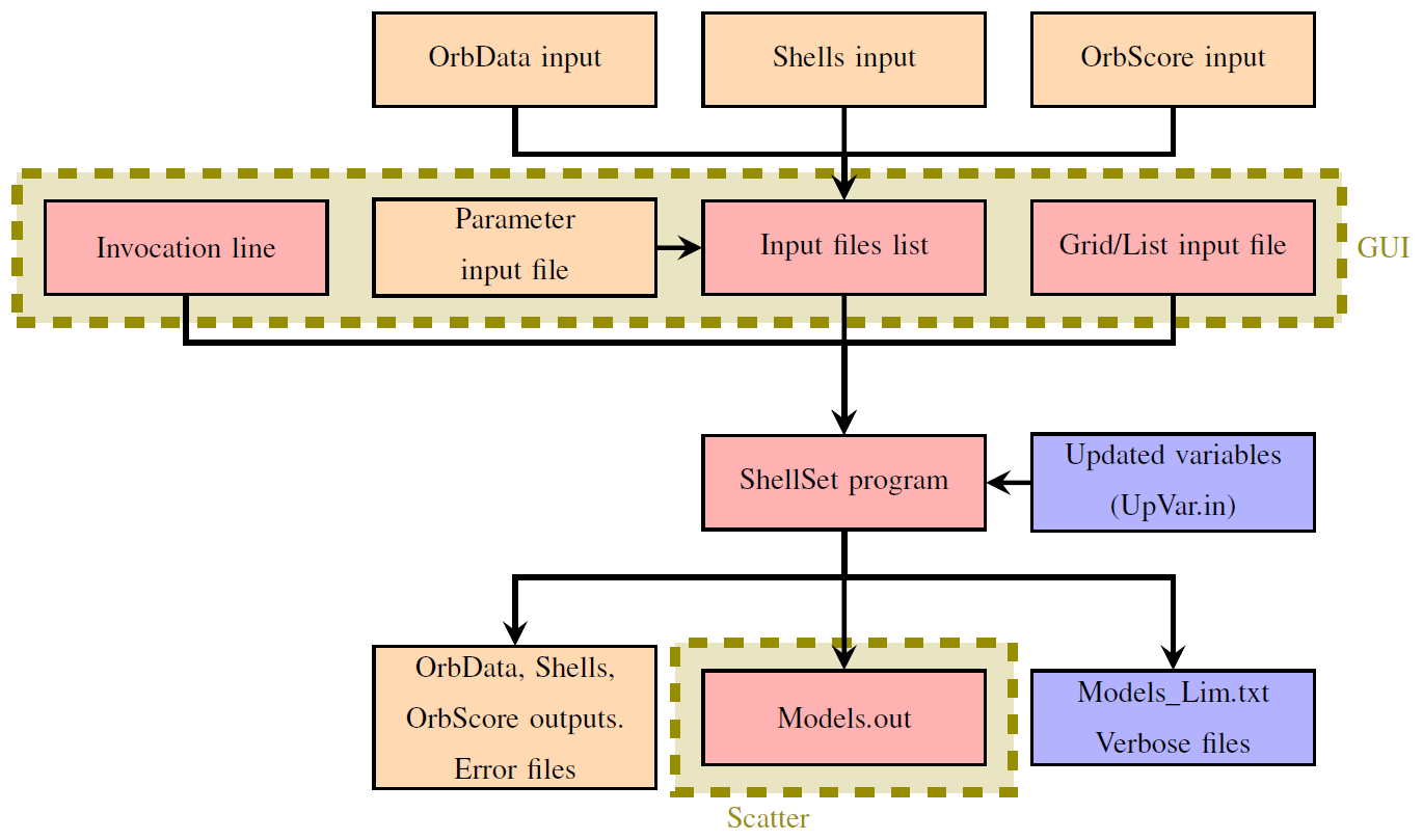
Figure 2 Simplified ShellSet schematic. The blue boxes show optional IO, the orange boxes show IO from the original programs, and the red boxes show new ShellSet functionality. Optional output is switched on at runtime, while optional input is switched on by its presence. The parts shown in the shaded dashed box labelled “GUI” can be handled by the provided GUI. Only the Models.out file may be plotted using the provided Python scatterplot routine.

The simplified input and initialisation user interface has three parts: (1) an input file for the model generation option (list or grid search), (2) an input file containing a list of input filenames for each of the original programs and (3) a selection of command line arguments which provide runtime information to ShellSet. These are visible in the three red boxes within the dashed olive box labelled “GUI” in Fig. 2. The input file names for each of OrbData, Shells and OrbScore are stored in the input file list, which combines with the invocation line and a model input file to initialise a ShellSet test. These steps, while providing the same input required by the individual programs, remove the user's control over any files that are at the interface between OrbData, Shells and OrbScore as well as between iterated Shells runs, removing the possibility of errors or delay after program initiation.

Certain experiments require the iteration of the Shells program, with each subsequent iteration requiring a file generated by the previous one. ShellSet is able to handle this for the user. The iteration of Shells is not exact in how many iterations could be required. For example, in Bird et al. (2008), three to five iterations were used, depending on the behaviour of the result after each iteration. Due to this we have added an option to exit the Shells iteration loop early. This exit may be performed if any two consecutive Shells iterations have misfit scores that are equal within a pre-selected tolerance. When activated, ShellSet expects a decimal input at runtime which represents the percentage change from the previous iteration (e.g. 10 % = 0.1). This is used to generate a range from the result of the previous model inside which the new model is deemed close enough. Since this is an optional feature, there is no default value, and the user is expected to provide one when activating it. A good value will depend on any requirement for subsequent results to be similar, on the scoring dataset used, and on the underlying problem. The ability to exit this iteration loop early has the potential to save a lot of time over an entire test. For example, if all 18 models of Bird et al. (2008) required five iterations, this would total 90 Shells runs, but if each required three iterations, there would only be 54 runs, i.e. a saving of 40 % on model numbers.

Along with this option, there are eight further command line arguments which allow the user to personalise the test at run time. These eight arguments allow the user to define the maximum iterations of Shells within the iterative loop, choose between the List and Grid input options, name a new directory where all IO files will be stored, and optionally set ShellSet to abort if any ignorable error is detected. For example, by default, if any FEG node exists outside a scoring data input grid, ShellSet will extrapolate the required value without calculation error but report an ignorable error. Activating this option will cause this issue to abort the program. Furthermore, the command line arguments allow a user to optionally produce extra program information in a new output file, select the misfit type used to select best models, create a special output file to store models with misfit scores better than a specified value, and optionally specify a misfit score at which the grid search algorithm will stop.

ShellSet also contains a geometric mean of misfit scoring option which can be used to rank models. This geometric mean, which users of OrbScore would have to calculate manually after each model has completed, can be comprised of any set of the five misfits generated: SSR, GV, SD, SA and FSR. Since SC is a score (larger is better) and not a misfit (smaller is better), it should not be included in this geometric mean. See Table 1 for information on the error types and Eq. (1) for the definition of the geometric mean.

By default, the geometric mean is always calculated by ShellSet using all or any of the five noted misfits which are calculated and reported in the output file. It may also be used to rank the models within the grid search by using the relevant command line argument at runtime and defining which misfits to use in its calculation.

Included within the ShellSet package but separate from its main work, there are two new Python programs which improve the usability of the program when compared to the stand-alone originals. First, we include a simple GUI which helps the user to create or update key input files and select runtime options before launching ShellSet. The GUI helps the user to update the files related to the parameter input values, the input file list as well as the list and grid input files. It also aids in the creation of a suitable invocation line (see the GUI box in Fig. 2). It contains checks on some typical errors for both file editing and program initialisation. The GUI dramatically simplifies the program setup and launch for new users, while more experienced users can choose to manually edit the input files using any text editor before launching from the terminal as with Shells. Second, we add a plotting routine that can generate 1D, 2D or 3D scatterplots from the main ShellSet output file. Plots generated by this routine can be seen in Figs. 3 and 5.

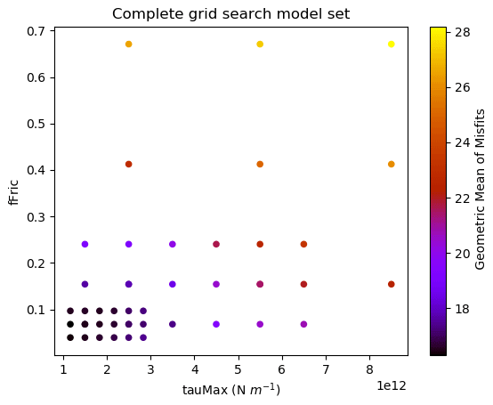
Figure 3 Visualisation of the grid search model set generated by ShellSet. The best results are found in the lower-left corner of the search area, corresponding to lower values for fFric and tauMax. This plot was generated with ShellSet's included Python scatter plotter.

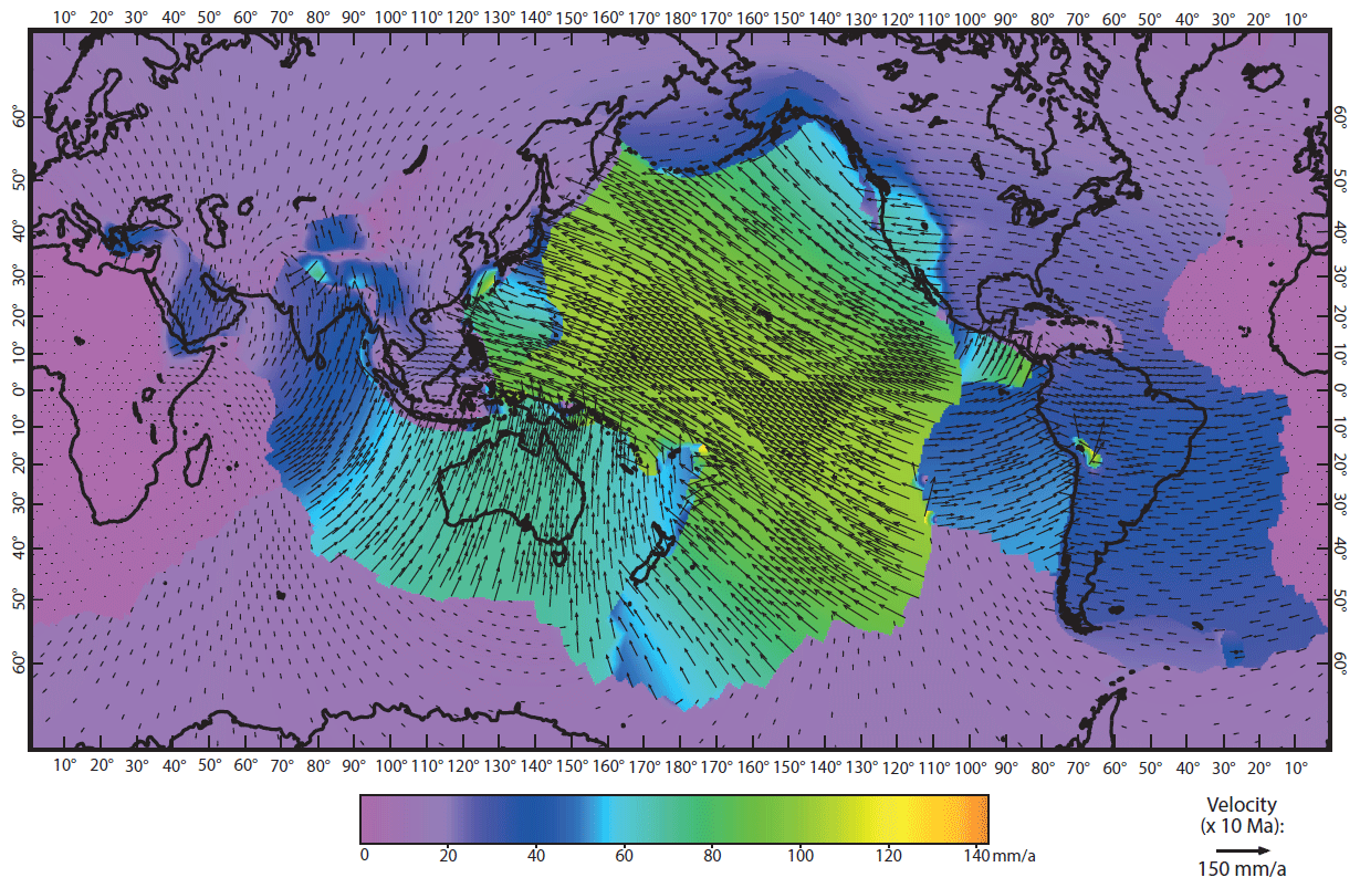
Figure 4 Surface horizontal velocity field of model 29.

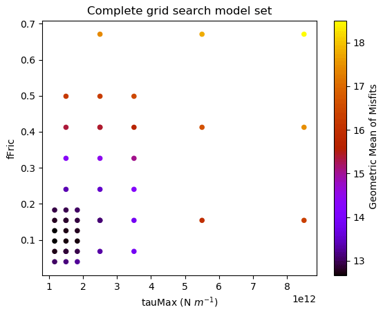
Figure 5 Visualisation of the grid search model set generated by ShellSet. The best results are found in the lower-left corner of the search area, corresponding to lower values for fFric and tauMax. This plot was generated with ShellSet's included Python scatter plotter.

This combination into a single program and the aforementioned updates have reduced errors related to manual control of the original individual programs. The ability to run models in parallel has saved us and our collaborators valuable research time, allowing the exploration of multiple research hypotheses in a shorter time. Performance analyses using two different compute machines are shown in Sect. 5.2.

4 Real-world examples

We now present two real-world example uses of ShellSet and its grid search option. Both examples follow the same path as in Bird et al. (2008) and search a similar 2D parameter space. All files for both examples are included with the ShellSet package download: see the Code and data availability section.

The first example is a direct comparison between the original results in Table 2 of Bird et al. (2008) and our automated search. In the second example we have added an extra dataset used to score the models that was not available in Bird et al. (2008). While Bird et al. (2008) had to manually update the parameters within the input files to run their simulations, we will use ShellSet's grid search to analyse a comparable parameter space that we define as [0.025, 0.8] for fFric and [1E12, 1E13] for tauMax (N m⁻¹).

In the first example, the geometric mean of misfits in Eq. (1) is comprised of the SSR, GV, SD and SA datasets as in Bird et al. (2008). The second example expands the geometric mean of misfits to include the new FSR dataset. Information on all misfit types and the geometric mean can be found in Sect. 2.3.

Due to changes in software since 2008, we expect different results to be calculated for the same models. Specifically, there have been minor updates to the original software and third-party libraries since the publication, which will affect its results, while there have also been numerous updates to the compilers used in the intervening years. Furthermore, ShellSet is compiled to run on the Linux OS, whereas the original results were obtained on a version compiled to run on the Windows OS. These differences will lead to, for example, different handling of variable precision at minor decimal places, which, over multiple iterations, will compound to alter model results in minor but noticeable ways. In order to account for these differences, we have re-run the previous best model (see model Earth5-049 in Table 2 of Bird et al., 2008) and reported the updated results in each example named New Earth5-049.

Preliminary testing showed that the requirement of relative velocity convergence to within 0.0001 was too strict for ShellSet; this is likely due to the aforementioned software differences. This gave us choices regarding the linear system solution iterations. We could alter the tolerance limit, increase the number of allowed iterations from 50, or both. We decided to loosen the tolerance to 0.0005 while keeping the iterations set to 50 in order to complete all the models in a reasonable time.

As in Bird et al. (2008), each model begins with a trHMax limit of 0.0 Pa for the first call of Shells before updating the limit to 2 × 10⁷ Pa. Parameter trHMax defines the upper limit of basal shear tractions, so an initial value of 0.0 means that the first iteration of Shells imposes no basal shear tractions.

A detailed analysis of the results is not within the scope of this work. However, for each example we will offer some observations and a basic analysis.

4.1 Using ShellSet to recreate Bird et al. (2008)

In this first example we show a recreation of the work done by Bird et al. (2008) using ShellSet.

Our grid search was set up to perform four iterations of Shells before a final call with updated boundary conditions, for a total of five Shells iterations per model. After the final run, OrbScore was used to generate misfit scores and the geometric mean of misfits for each model, which were used to rank the models. The geometric mean of misfits, from Eq. (1), for this example is given as

$$\begin{array}{}\text{(2)}& \mathrm{GM}=\sqrt[\mathrm{4}]{S_{\text{SSR}}{S}_{\text{GV}}{S}_{\text{SD}}{S}_{\text{SA}}}.\end{array}$$

The grid search partitioned the domain into nine cells in a 3 × 3 grid, with each cell represented by its central model. The two best models of these nine were then chosen to continue to the second level, where each represented cell is further divided into a 3 × 3 grid. This was repeated with the 18 models at this second level to generate another 18 models. This three-level grid search gives a total of 41 distinct models once the four repeated models are excluded, together with a final resolution of $\mathrm{1}/\mathrm{27}$ of the original ranges (from 9 × 10¹² N m⁻¹ and 0.775 to 3.3 × 10¹¹ N m⁻¹ and 0.0287) for tauMax and fFric, respectively.

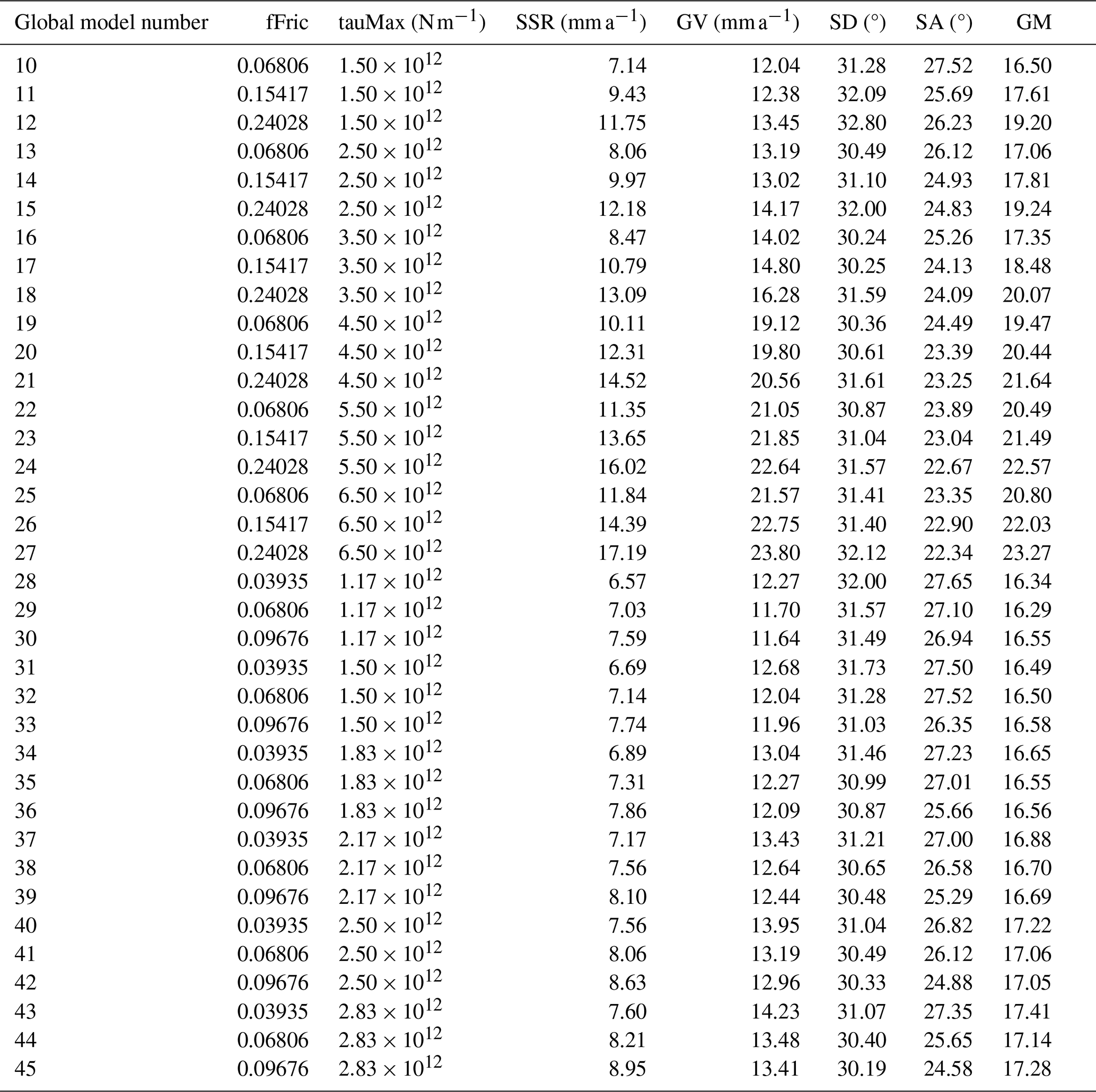
Table 2 Previous best model of Bird et al. (2008), Earth5-049, compared with the ShellSet grid search models. New Earth5-049 is an exact re-run of Earth5-049 to account for differences in hardware and software. The best model, using the geometric mean score, is shown in bold text.

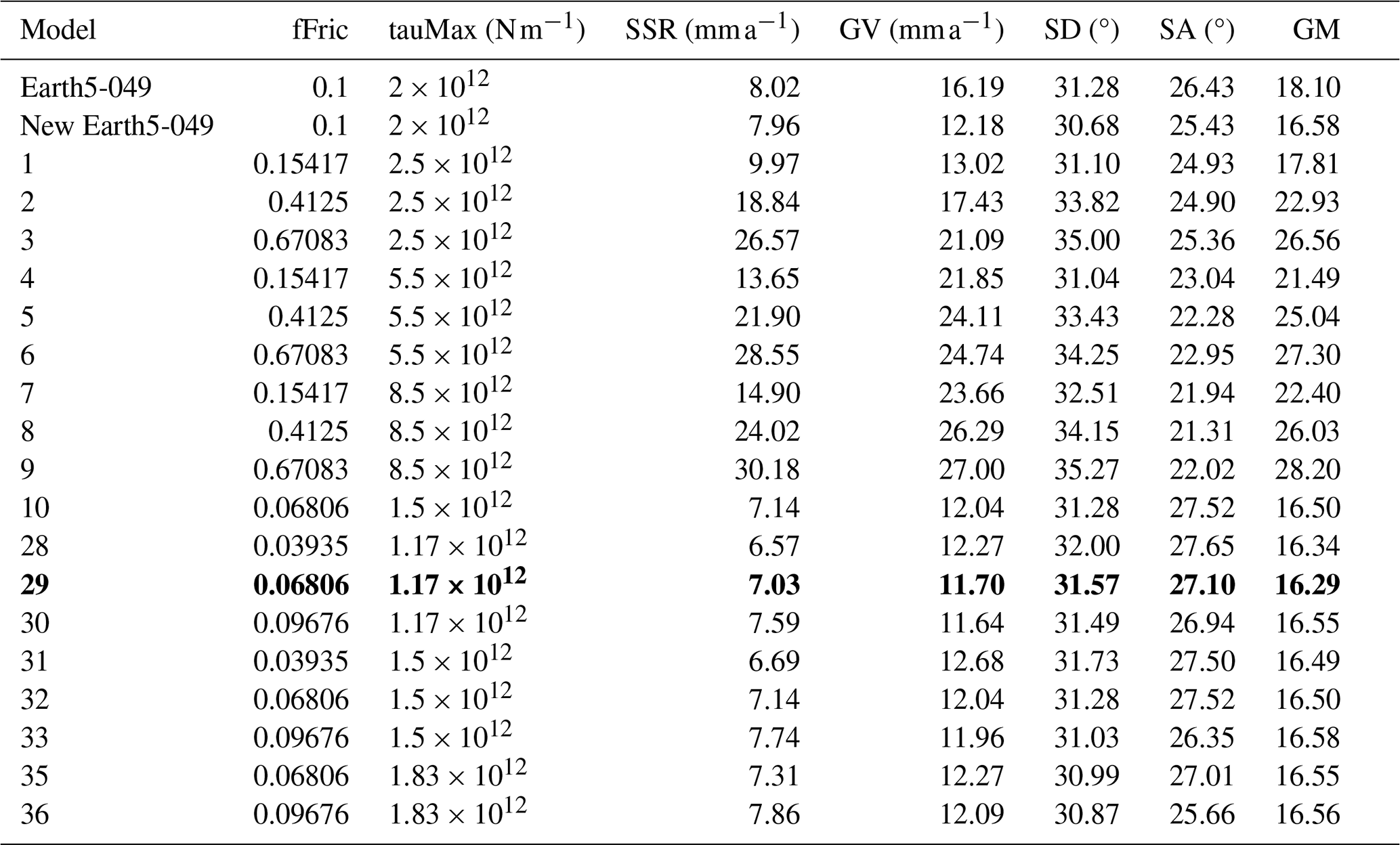
Misfits are reported to two decimal places but are calculated to greater accuracy. The misfit types are SSR, GV, SD and SA. The geometric mean (GM) is calculated as in Eq. (2).

Table 2 shows some of the results we have obtained using ShellSet. The first two rows show the previous best model, Earth5-049, and the scores when this model was re-run as New Earth5-049. For brevity, we only report the models at the first level to demonstrate the initial grid (models 1–9) and then every model for which the geometric mean of misfits is better than New Earth5-049. The entire search history, excluding the first level, can be seen in Table B1 of Appendix B.

It is immediately clear that, within the first nine models, the best geometric mean results are obtained with a minimum fFric and tauMax within their respective ranges, with fFric being the more important of the two. This is made clearer in Fig. 3, which maps the entire grid search.

There are eight distinct models (model 32 being a repetition of model 10) that obtained an equal or better geometric mean of misfit scores than New Earth5-049. Each one of these eight models achieved a better SSR score than New Earth5-049. Five of the eight have a better GV score (models 10, 29, 30, 33 and 36), but none of them has a better score in either SD or SA. The absolute best model is model 29, with a geometric mean of 16.29 (an improvement of 0.29).

Examining the full set of models within this test, using Tables 2 and B1, we can see that over the entire model set no single model has better or equal results in more than two of the four individual scores that comprise the geometric mean when compared to New Earth5-049.

Although a detailed analysis of these results is beyond the scope of this work, we have plotted the horizontal velocities of model 29 in Fig. 4 for comparison with Fig. 10 of Bird et al. (2008). We can immediately see that our new model has a lower maximum horizontal velocity than Earth5-049, with a maximum of a little over 140 mm a⁻¹ compared to 153.9 mm a⁻¹. Interestingly, we can clearly see an increase in velocities around Nepal from approximately 40 mm a⁻¹ to approximately 60 mm a⁻¹. With all other inputs being equal between the two models, these differences are caused solely by the updated values of fFric and tauMax.

4.2 ShellSet with an additional fault slip rate dataset

The second example performs the same test as the first example, with an added dataset that defines the FSR; see Appendix A for further information on this dataset. We note that the fault slip rate dataset was not available in Bird et al. (2008).

This additional dataset was used to generate an extra misfit for each model, which was then used within the calculation of the geometric mean of misfits as in Eq. (1), which becomes

$$\begin{array}{}\text{(3)}& \mathrm{GM}=\sqrt[\mathrm{5}]{S_{\text{SSR}}{S}_{\text{GV}}{S}_{\text{SD}}{S}_{\text{SA}}{S}_{\text{FSR}}}.\end{array}$$

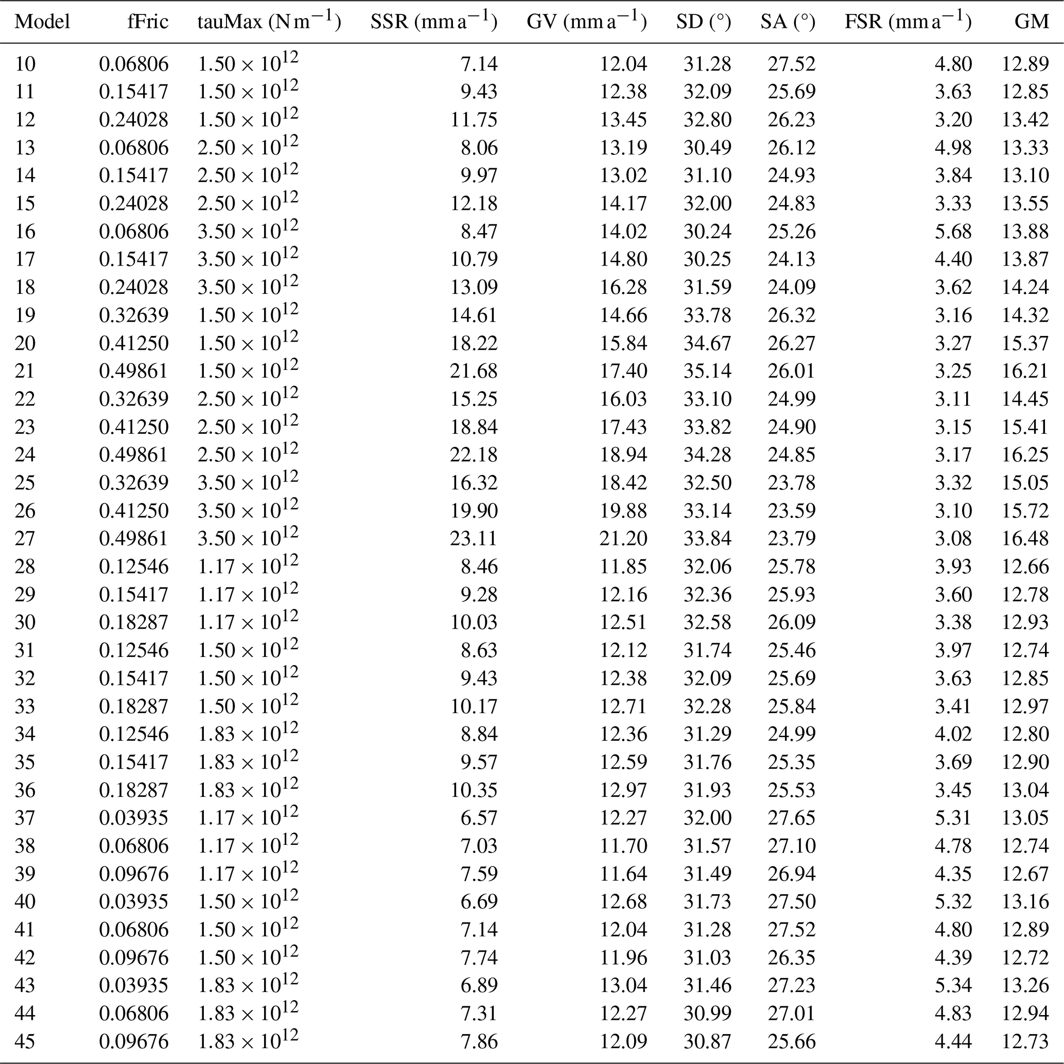
Table 3 The previous best model of Bird et al. (2008), Earth5-049, and example 1 compared with the ShellSet grid search models. New Earth5-049 and New Ex1 29 are exact re-runs of Earth5-049 and the best model of example 1, respectively. The best model, using the geometric mean score, is shown in bold text.

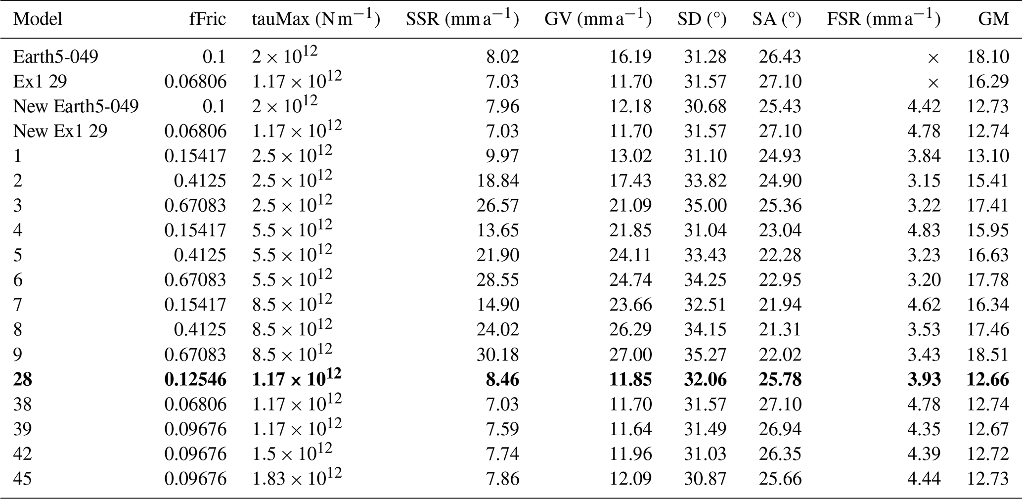
Misfits are reported to two decimal places but are calculated to greater accuracy. The misfit types are SSR, GV, SD, SA and FSR. The GM is calculated as in Eq. (3).

In the first two rows of Table 3, we report the best model of Bird et al. (2008) (Earth5-049) and the best model of example 1 (Ex1 29). We re-run these two best models, adding the new FSR dataset to generate the fair comparison models New Earth5-049 and New Ex1 29, respectively.

As in example 1, the search favours lower values for fFric and tauMax. However, in this example, the more important variable is tauMax. This search has generated four models that are an improvement on or equal to New Earth5-049 and New Ex1 29 (see models 28, 39, 42 and 45), with model 38 being a repeat of Ex1 29. The addition of the fault slip rate scoring dataset has meant that every model has a better geometric mean score than example 1 (see Table 2). The absolute best model is model 28, with a geometric mean that is 0.07 lower than New Earth5-049 and 0.08 lower than New Ex1 29.

Although, as noted, every model run in both examples 1 and 2 has a lower geometric mean score in the second example, not every reduction is equal, and so the alteration to the geometric mean has caused alternate models to be selected between the levels. This alteration takes the grid search through a different path to find its optimal model. We will now outline where the deviations within the search paths occur.

In example 1 the two best models of the first level are models 1 and 4 (see Table 2), while in example 2 the best models are models 1 and 2 (see Table 3). Since all other misfit scores remain equal between the two examples, this change from selecting model 4 to selecting model 2 is wholly caused by the addition of the fault slip rate dataset altering the geometric mean score calculation. The best models at the second level are also, by chance, run in both examples. In the first example these models are models 10 and 13, while in the second example they are models 10 and 11 (see Tables B1 and B2). The best model in the second example is not run in the first example: this is an effect of the updated geometric score calculation.

As in example 1, we have plotted the horizontal velocities of the best model (model 28) in Fig. 6 for simple comparison with Figs. 4 and 10 of Bird et al. (2008). This model shows a further reduction in the maximum horizontal velocity to approximately 137 mm a⁻¹ and, unlike in example 1, shows velocity magnitude results around Nepal that are similar to Bird et al. (2008).

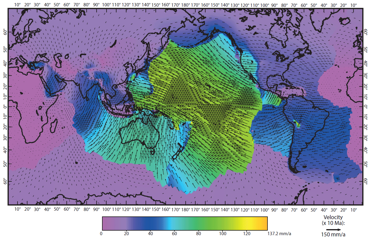
Figure 6 Surface horizontal velocity field of model 28.

By comparing our two examples, we can see that, even though the best models are those with minimum fFric and tauMax, the addition of the fault slip rate dataset causes the grid search (in this 2D fFric–tauMax space) to prefer models with a lower tauMax value.

5 Performance analyses

In this section we demonstrate two different performance tests used to check the performance of ShellSet. Firstly, we test the effect on both the total program and the solution routine time when changing the number of MKL threads. Secondly, we analyse the program performance when running multiple models in parallel. All performance results reported in this section are an average of three repeats of equal performance tests. Each section uses an equal model for each of its tests, and this model is consistent over all the sections.

5.1 MKL performance testing

We first test the effect that altering the number of threads available to the MKL routines has on both the routine itself and the total program time. We focus this analysis on the dgbsv routine as this is iteratively applied to the complete system of equations representing the finite-element grid (16 008 × 16 008 in our global example), whereas the dgesv routine is used to solve a 3 × 3 system.

In order to analyse the effect of the MKL thread number, we perform an experiment using a single model iterated twice on a single core (using a single MPI process), varying only the number of threads available to the MKL routines. Within an MKL routine the number of threads used includes the core working in serial, so a team of 64 MKL threads is the serial running core plus an extra 63 threads.

Table 4 Performance tests using a 64-core node. All the simulations were performed using a model on a single node, varying only the number of MKL threads. The time, in seconds, and the speedup are reported to two decimal places.

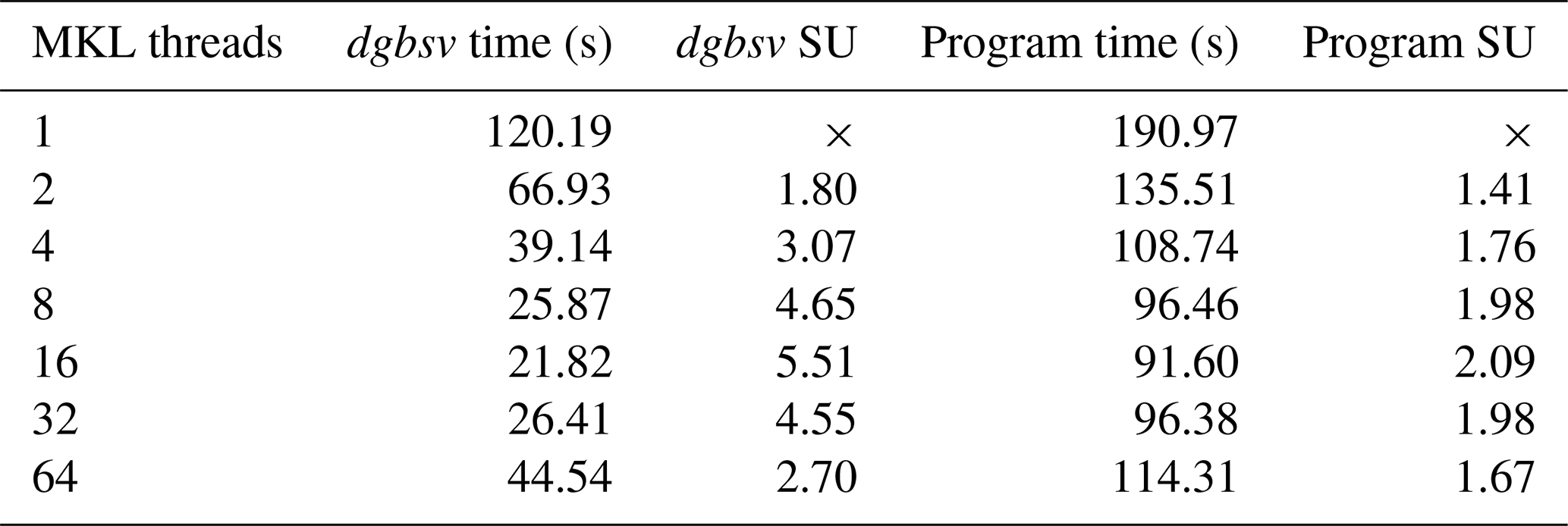
Tests were performed on a four-socket system equipped with four Xeon Gold 5218 CPUs, which are 16-core or 32-thread chips.
× SU is not calculated for the serial run as it will always be 1.

The experiment was performed on a single 64-core node of the HPC cluster at INGV Rome. We use a single node as MKL threads work in a shared-memory environment and so cannot be divided across multiple nodes. Table 4 shows the time taken and the calculated speedup (SU) for both the entire program and the dgbsv routine for the model when run with 1-64 MKL threads, while Fig. 7 plots these results.

Figure 7 Speedup plot for the dgbsv routine and program using 2-64 MKL threads.

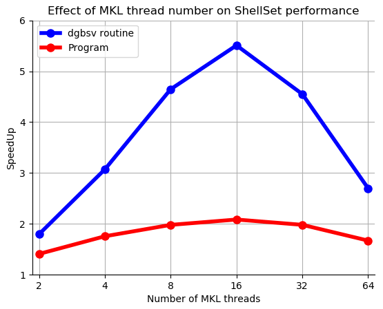
Looking at Table 4, we can see that increasing the number of MKL threads does improve the performance over a single model, up to a point. Increasing the number of MKL threads from 1 to 16 would see a speedup of approximately 5.5, reducing the time spent inside the MKL routine from 120 to 22 s and accordingly reducing the time of the entire program by approximately 100 s, which is not insignificant for a single model. Furthermore, this would add up to a significant amount of time saved over a large number of models. Adding extra threads to the MKL routines beyond 16 began to degrade the performance, potentially due to the fact that the HPC node is comprised of four CPUs with 16 cores, and so using more than 16 threads would mean performing calculations across CPU boundaries. This can degrade the performance by requiring cross-socket (inter-CPU) memory access and thread barriers, which can give a reduced performance relative to using a single CPU.

5.2 MPI performance testing

ShellSet causes no appreciable delay when individual components are compared to the three original programs, as the underlying software is not changed. However, the inter-program links within ShellSet offer two opportunities for a performance increase when compared to the original program. Firstly, the total simulation time of each model is reduced thanks to the removal of the user interface during simulations. Secondly, the MPI framework made possible by these new links allows numerous models to be run in parallel. We now provide an analysis of these two enhancements.

5.2.1 Performance gain from removing the user interface

Removing the need for a user interface between the formerly independent program units decreases the time required to complete any model or set of models. The links, which would otherwise require a user to feed output from one program into the next, are now performed automatically by ShellSet. Comparing the time taken by ShellSet to utilise these links to a user is a tricky task as the time taken depends on the user and their abilities, so this is not something which we will show. However, we report the following comparison from our experience.

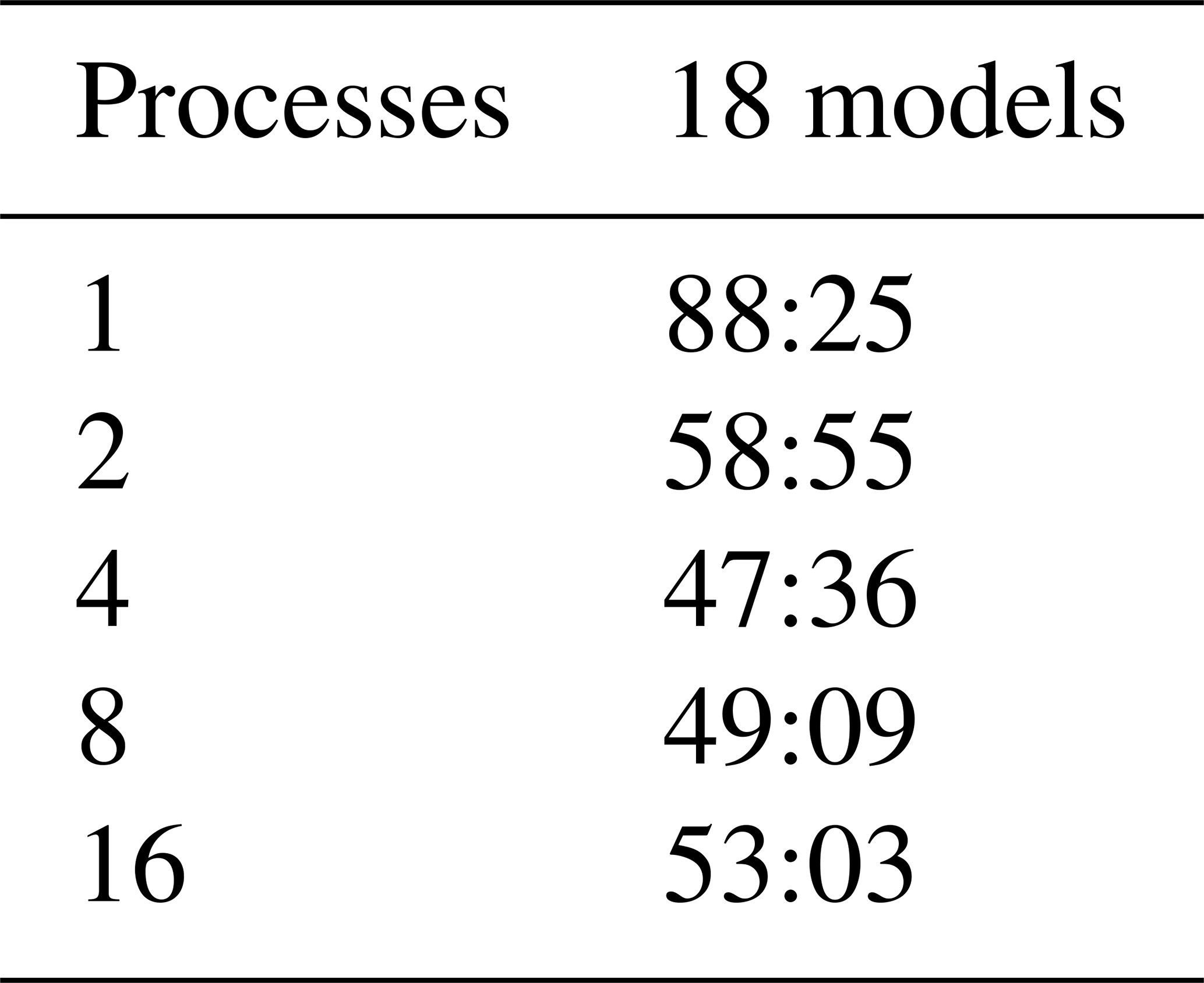
Table 2 of Bird et al. (2008) shows 18 models in which the fFric and tauMax variables were varied. Each model required one run of OrbData, four to five iterations (as stated in the text) of Shells and one run of OrbScore. With all file IOs controlled manually by the user, these 18 models (72–90 Shells runs) took 4 d to 1 week when performed in a serial manner. We performed a realistic test where we alter the number of both MPI processes and MKL threads, testing the performance over 18 models on a desktop machine.

Following the approach outlined in Bird et al. (2008), each timed model consists of using OrbData to perform an update to the finite-element grid, four Shells iterations, a fifth Shells iteration (using updated boundary conditions) and a single OrbScore run to score the final run. We use a model that we know completes fully, meaning it converges within the user-defined MKL iteration limit and passes all input variable criteria.

Table 5 Performance test using an Intel Core i9-12900 2.4 GHz CPU desktop with 64 GB RAM, 16 physical cores (8 performance cores, 8 efficient cores) and 24 threads. The times are reported to the nearest second (mm:ss).

One worker uses six MKL threads, 2 workers use four MKL threads, 4 workers use two MKL threads, and 8 and 16 workers use one MKL thread.

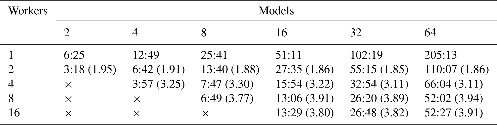
Table 5 reports the time taken for various MPI process and MKL thread pairings to perform 18 models. It shows that ShellSet is able to perform 18 models with five Shells iterations in less than 90 min and as fast as 48 min. Although the results shown in Table 5 were obtained from more recent hardware and software, a large portion of the time taken for the 18 models of Bird et al. (2008) was lost to the user interface and times when the user was not present – these are not issues with ShellSet.

5.2.2 Performance gain from parallel models

The use of an MPI framework provides a second opportunity for performance improvement by allowing multiple models to be run in parallel. This can be tested in a more traditional fashion by comparing the time taken to complete a given number of models using a given number of processes. We also report the ratio between the serial and parallel times, known as the speedup.

For simplicity, the tests were performed over a single search level of a 2D parameter space, varying the number of models and the number of worker processes. We do not report the results where the number of processes is greater than that of the models, as ShellSet contains a check on the number of models and worker processes to prevent an over-allocation of compute resources. In reality, it would likely have a negative effect by unnecessarily tying up compute resources. For these tests we have fixed the number of MKL threads to one in order to maximise the number of cores available for MPI processes. We have also fixed all the models to be equal (after the model generation procedure) in order to be able to more fairly compare the timing results across all the numbers of the models, the processes and both machines used. Each of the tests iterates the Shells solution procedures twice.

Table 6 Performance test using an Intel Core i9-12900 2.4 GHz CPU desktop with 64 GB RAM, 16 physical cores (8 performance cores, 8 efficient cores) and 24 threads. Each time is reported to the nearest second (mm:ss) and is an average of three tests. The speedup, shown in brackets, is calculated using seconds to five decimal places but is reported to two decimal places.

All simulations were performed with the number of threads used within MKL routines fixed at one.
× Test setups with more workers than models are not performed.

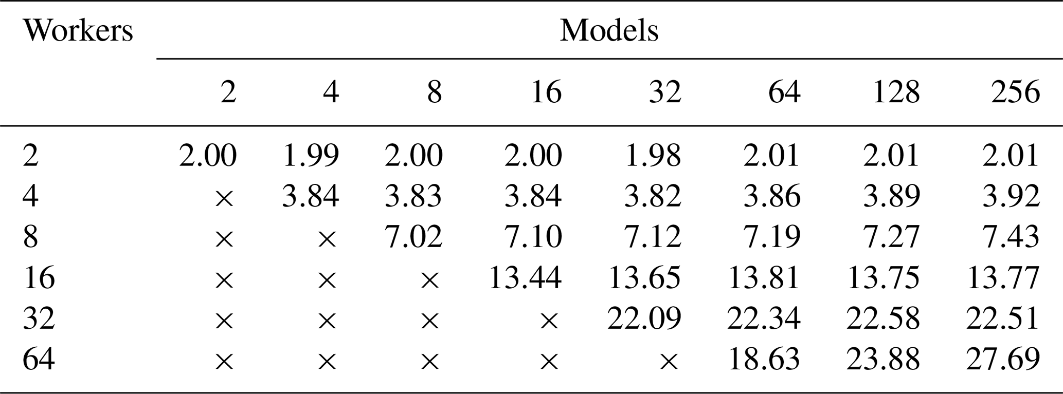
Table 6 reports the time in minutes and seconds for the test performed on a typical desktop computer. The bracketed entries are the speedup compared to a single worker. Table 7 reports only the speedup for the test carried out on a 64-core HPC node. We calculate the SU using

$$\mathrm{SU}={\displaystyle \frac{T_{\mathrm{s}}}{T_{\mathrm{p}}}},$$

where T_s is the time taken by a single worker and T_p is the time taken by multiple workers.

The speedup values reported (bracketed) in Table 6 are around 2–4. In fact, the speedup results for two and four processes are very reasonable at approximately 1.9 and 3.3, respectively. Increasing the number of processes beyond this however yields very little in extra speedup and eventually a decrease in performance (see Fig. 8 for a plot of the speedup). This could be because this computer is relatively small (with eight performance cores and eight efficient cores), and increasing the number of processes starts to strain the system. By increasing the number of MPI processes performing models in parallel without increasing the total machine size, we increase the load on the memory bandwidth. This will eventually cause a transition from a compute-bound situation to a memory-bound situation, which would seem to occur between four and eight MPI processes and would then explain the levelling-off performance after eight processes. It is also the case that this test was performed in a WSL2 Linux environment hosted in Windows, and therefore we cannot be certain about the true availability of the cores since there will be some background OS work related to Windows, not least of which is the running of the WSL2 environment.

Figure 8 Speedup plot for 2, 4, 8 and 16 workers performing 16, 32 and 64 models, on a desktop machine. Values are given (in brackets) in Table 6.

Since the general user does not usually worry about speedup results and instead focuses mostly on time, and despite poor speedup results for a larger number of processes, the results using up to four and even eight processes are very interesting. The small increase in performance between four and eight processes is worth considerable time-saving when calculating 64 models with roughly 14 min saved and calculating 32 models with over 6 min saved.

Table 7 Speedup results from performance tests using a 64-core node. The node is a four-socket system equipped with four Xeon Gold 5218 CPUs, which are 16-core or 32-thread chips. The speedup is calculated using seconds to five decimal places but is reported to two decimal places.

All simulations were performed with the number of threads used within MKL routines fixed at one.
× Test setups with more workers than models are not performed.

The speedup values reported in Table 7, which shows results obtained on a single HPC node, range from 2 to almost 30. The speedup results for 2, 4, 8 and 16 processes are very good at approximately 2, 3.8, 7.2 and 13.6, respectively, remaining close to the ideal values. As in Table 6, increasing the number of processes beyond this started to see less increase in performance, but not to the same extent. Even at 32 processes, the speedup is reasonable at approximately 22. We only see poor performance at 64 cores – when the node is full. Figure 9 shows a plot of the speedup values. Interestingly, we can see that, unlike in Fig. 8, where the three plots have the same behaviour, in Fig. 9 the behaviour is equal until the node is full, when we see quite a large difference in the performance between the three plots. This is possibly a symptom of the number of models performed within the test, where running more models hides some poor performance as a result of some models taking longer than others to complete, although this would likely be borne out in other results as well. Another possibility is a more general unpredictability when a compute node is full.

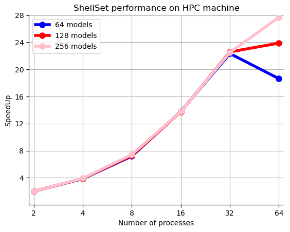
Figure 9 Speedup plot for 2, 4, 8, 16, 32 and 64 workers performing 64, 128 and 256 models, on a 64-core node of a HPC machine. Values are given in Table 7.

We can see in these results the benefit of a larger, and dedicated, compute system compared to a smaller hosted environment, with the speedup results of Table 7 remaining much closer to the ideal value for longer. One possible reason for the slowdown of the performance increase, seen between 16 and 32 MPI processes, is that, as noted in relation to the previous MPI performance example, we are increasing the load on the memory bandwidth and possibly transitioning from a compute-bound situation to a memory-bound situation. A reason for this levelling-off performance occurring in a higher number of MPI processes, in comparison to the first MPI performance test, could be that the HPC system has a higher memory bandwidth. It is also true that there will be fewer interfering background processes on a dedicated compute system compared to WSL2 hosted in the Windows OS.

The two tests using two different types of Linux environment on two different machines prove that there is considerable time to be saved by running models in parallel. Our tests have shown results which are 4 times faster on a typical desktop machine and almost 30 times faster using a dedicated compute node.

In general, searching algorithms which contract through levels such as the grid search could suffer from performance loss at the interface between the end of one level and the beginning of the next. Indeed, the grid search employed in ShellSet would suffer from such a degradation. However, the examples shown use a single level to generate the number of models required, and so this would not be present in these performance results.

Taken together, the results of the MKL and MPI performance experiments suggest that, at least for our example global model, it is more important to run many models in parallel rather than fewer highly parallel models. Since the speedup performance shown in Table 4 quickly falls away from the ideal value (whereas the speedup results shown in Tables 6 and 7 remain close to the ideal value), we can see that the most important aspect of parallelism for ShellSet is a multi-model approach. Trivially, when running a relatively small number of models on a large enough machine, the most sensible approach is likely to be a combination of the two parallel schemes by performing multi-threaded MKL routine calls in parallel. We note that the best approach will depend on the underlying model size, its complexity as well as the size and technical characteristics of the compute machine, all of which will be personal to the user.

6 Conclusions and future work

This article has outlined a new MPI parallel dynamic neotectonic modelling software package, ShellSet, which has been designed for use by the wider geodynamic modelling community. The simplified hands-off nature of ShellSet reduces user–program interactions to a minimum, while the addition of a GUI further simplifies those remaining interactions. These improvements open ShellSet up to a less experienced user and reduce setup errors for all users.

We showed in Sect. 4 two examples of ShellSet's abilities within the target field of study by first improving on an existing global model developed in Bird et al. (2008), and then we further improved on that with the addition of a new dataset of fault slip rates. Both examples were completed in a fraction of the time taken to generate the existing global model of Bird et al. (2008).

In upcoming work, ShellSet will be used to optimise the rheology of the lithosphere in the Apennine region for better dynamical simulations of neotectonics and the associated seismicity. We also plan to use ShellSet in work forming predictions of seismic hazard within the central Mediterranean region.

ShellSet was developed and tested on a computer with widely available capabilities. We have demonstrated that ShellSet achieves improved performance (relative to the original software) and speedup when running multiple models in parallel on both typical and larger HPC machines (see Sect. 5). Despite the improved performance, in Sect. 5 we noted potential reasons for the levelling-off performance when running multiple models in parallel, one of them being that we may be crossing from a compute-bound to a memory-bound situation. The grid search algorithm could also cause performance loss at the transition between contracting levels, however our tests did not analyse this possibility. An analysis of parameter space sampling methods, as done in Reuber (2021), could yield a method which would allow ShellSet to better utilise its parallelism, particularly on HPC machines. One candidate method is the NAplus algorithm (Baumann et al., 2014), which was shown to scale well and which is built on the well-known Neighbourhood algorithm introduced in Sambridge (1999). Another is a random walk sampling performed using multiple parallel and independent random walks. While these sampling methods would not solve the issue of performance loss when transitioning to a memory-bound situation, more efficient HPC machine use would enable the parameter space to be searched to a finer level and would provide faster results, and the improved use of larger HPC structures would allow use of much larger (in terms of memory) models.

Appendix A: Fault slip rate (FSR) dataset

Here we outline the process followed to create a usable FSR dataset, as used in example 2 of Sect. 4.

In Styron and Pagani (2020), the authors report a global active fault database of approximately 13 500 faults collected through the combination of regional datasets. They note that approximately 77 % of the faults have slip rate information: this provided us with 10 395 estimated initial faults for potential use in our work.

Due to the requirements of our program, the database needed some cleaning. Of the approximately 13 500 initial fault traces, around 9500 faults either have no offset rate or lack upper and lower limits which identify a rate based on a dated offset feature (unbounded rates are model rates, which we do not consider to be data). A further 684 lack rake information, and 1022 fault traces lack the necessary dip information. After discounting these fault traces, we were left with 2487 traces, which might be used in OrbScore if each aligns with a fault element of the current finite-element grid.

Those fault traces remaining are mostly located in one of four areas: the Mediterranean–Tethyan orogenic belt, well-covered from Portugal to Pakistan; Japan; New Zealand; and California. Many of these almost 2500 fault traces (e.g. those in Japan) did not correspond in position (and orientation) to any of the fault elements of the existing finite-element grid as used in Bird et al. (2008). Therefore, they were also removed from our dataset.

Remaining fault traces were subjected to the following two comparison filters with respect to the finite-element grid of 2008: firstly, the overall azimuth (endpoint to endpoint) of the fault trace must be within a ± 15° tolerance of the grid fault element azimuth; secondly, the shortest distance from the fault trace to the grid fault element must be less than one-eighth of the length of that fault element.

After applying these conditions to the fault traces, we were left with 931 associations. Accounting for the fault traces of the database which match with multiple fault elements left us with 572 faults.

The fault elements of the finite-element grid file that have multiple associations within the new dataset needed to be controlled to avoid over-weighting of those elements with more associations. This was done by summing the product of the “adjacent” fault length (limited to the length of the fault element) with the offset rate for all the associated traces and then dividing the sum by the length of the fault element to get the aggregated offset rate that the fault element should match.

Appendix B: Tables related to demonstrated real-world examples

Table B1 Example-1 grid search results, excluding the first level, which is shown in Table 2.

Misfit types listed in Table 1.

Table B2 Example-2 grid search results, excluding the first level, which is shown in Table 3.

Misfit types listed in Table 1.