the Creative Commons Attribution 4.0 License.
the Creative Commons Attribution 4.0 License.
 | 31 Jul 2024
Bayesian hierarchical model for bias-correcting climate models
Erick A. Chacón-Montalván
Amber Leeson
Climate models, derived from process understanding, are essential tools in the study of climate change and its wide-ranging impacts. Hindcast and future simulations provide comprehensive spatiotemporal estimates of climatology that are frequently employed within the environmental sciences community, although the output can be afflicted with bias that impedes direct interpretation. Post-processing bias correction approaches utilise observational data to address this challenge, although they are typically criticised for not being physically justified and not considering uncertainty in the correction. This paper proposes a novel Bayesian bias correction framework that robustly propagates uncertainty and models underlying spatial covariance patterns. Shared latent Gaussian processes are assumed between the in situ observations and climate model output, with the aim of partially preserving the covariance structure from the climate model after bias correction, which is based on well-established physical laws. Results demonstrate added value in modelling shared generating processes under several simulated scenarios, with the most value added for the case of sparse in situ observations and smooth underlying bias. Additionally, the propagation of uncertainty to a simulated final bias-corrected time series is illustrated, which is of key importance to a range of stakeholders, such as climate scientists engaged in impact studies, decision-makers trying to understand the likelihood of particular scenarios and individuals involved in climate change adaption strategies where accurate risk assessment is required for optimal resource allocation. This paper focuses on one-dimensional simulated examples for clarity, although the code implementation is developed to also work on multi-dimensional input data, encouraging follow-on real-world application studies that will further validate performance and remaining limitations. The Bayesian framework supports uncertainty propagation under model adaptations required for specific applications, providing a flexible approach that increases the scope of data assimilation tasks more generally.
- Article
(7189 KB) - Full-text XML
- BibTeX
- EndNote


Climate models are invaluable in the study of climate change and its impacts (Bader et al., 2008; Flato et al., 2013). Formulated from physical laws and with parameterisation and process understanding derived from past observations, climate models provide comprehensive spatiotemporal estimates of our past, current and future climate under different emission scenarios. Global climate models (GCMs) simulate important climatological features and drivers, such as storm tracks and the El Niño–Southern Oscillation (ENSO) (Greeves et al., 2007; Guilyardi et al., 2009). In addition, independently developed GCMs agree on the future direction of travel for many important features, such as global temperature rise under continued net-positive emission scenarios (Tebaldi et al., 2021). However, GCMs are computationally expensive to run and also exhibit significant systematic errors, particularly on regional scales (Cattiaux et al., 2013; Flato et al., 2013). Regional climate models (RCMs) aim to downscale GCMs dynamically; represent climatology for specific regions of interest more accurately; and have parameterisation, tuning and additional physical schemes optimised for the region (Giorgi, 2019; Doblas-Reyes et al., 2021). Despite this, significant systematic errors remain, particularly for regions with a complex climatology and with sparse in situ observations available to inform process understanding, such as over Antarctica (Carter et al., 2022). These systematic errors inhibit the direct interpretation of climate model output, which is particularly important in impact assessments (Ehret et al., 2012; Liu et al., 2014; Sippel et al., 2016).
There are many fundamental causes of systematic errors in climate models, including the absence or imperfect representation of physical processes, errors in initialisation, influence of boundary conditions and finite resolution (Giorgi, 2019). The inherent complexity and computationally expensive nature of climate models make a direct reduction in systematic errors through climate model development and tuning challenging (Hourdin et al., 2017). Additionally, end users are typically only interested in a narrow aspect of the output (e.g. possibly only one or two variables), which the climate model is unlikely to be specifically tuned for. Post-processing bias correction techniques allow for improvements to the consistency, quality and value of climate model output specific to the end user's focus of interest, with a manageable computational cost and without the requirement for in-depth knowledge behind the climate model itself (Ehret et al., 2012). Transfer functions are derived between the climate model output and in situ observational data to correct components such as the mean (Das et al., 2022) or probability density functions (PDFs) of the data (Qian and Chang, 2021). This paper focuses on providing a novel framework for correcting systematic errors in the PDF of the climate model output at each grid point.
One of the fundamental issues often attached to post-processing bias correction is the lack of justification based on known physical laws and process understanding (Ehret et al., 2012; Maraun, 2016). The spatiotemporal field and associated covariance structure from the climate model, which is consistent with accepted physical laws, are typically not considered and therefore not preserved. Resulting corrected fields may exhibit behaviour that is too smooth or sharply varies over the region and has significant discontinuities near observations. In addition, many approaches to bias correction fail to adequately handle uncertainties or estimate them at all. Reliable uncertainty estimation is valuable to include in impact studies to inform resulting decision-making. This is especially true for regimes with tipping points, such as ice shelf collapse over Antarctica, where uncertainties in the climatology can cause a regime shift (DeConto and Pollard, 2016). In this paper, these issues are partially addressed through the development of a fully Bayesian hierarchical approach to bias correction. Parameter uncertainties are propagated through the hierarchical model, and underlying spatial covariance structures are captured with latent Gaussian processes (GPs) for both in situ observations and climate model output.
The approach presented builds on that of Lima et al. (2021), which models the in situ observational data as generated from a GP and uses quantile mapping (Qian and Chang, 2021) to apply the correction to the climate model output. In Lima et al. (2021), the spatial covariance structure of the climate model output is not considered and uncertainty is not propagated to the final bias-corrected time series. The novelty of the approach proposed here is that shared latent GPs are modelled between the climate model output and the in situ observational data, which is an attempt at incorporating information from the physically realistic spatial patterns of the climate model output in predictions of the unbiased field. Additionally, uncertainty is propagated through the quantile mapping step, which results in uncertainty bands in the bias-corrected output. The approach is developed with the focus on applying bias correction to regions with sparse in situ observations, such as over Antarctica, where capturing uncertainty in the correction is of key importance and where including data from all sources during inference is particularly valuable. Performance under simulated scenarios with differing data density and underlying covariance length scales is evaluated in this paper and the potential added value assessed when compared with the approach in Lima et al. (2021).
While simple simulated scenarios are focused on in this paper, the applicability of GPs for modelling complex spatial patterns seen in real-world climatology is already illustrated in Zhang et al. (2021) and Lima et al. (2021). The non-parametric nature of GPs makes the model flexible and able to capture complex non-linear spatial relationships. Additionally, features of GPs such as uncertainty estimation, sensible extrapolation, kernel customisation and ability to produce accurate predictions with limited data are desirable for real-world case studies. Finally, advancements in approximate inference methods have improved the scalability of GPs, improving the applicability to large climate data sets, as demonstrated in Wang and Chaib-draa (2017). In addition to the main results presented in Sect. 4, to further demonstrate the flexibility of the methodology presented in this paper and its applicability to potential real-world scenarios, some additional simulated scenarios are created, with added complexity, the results of which are presented in Appendix G. These additional scenarios test the robustness of the model on potential real-world situations, where not all the assumptions of the model necessarily completely hold.
Developing the bias correction approach in a flexible Bayesian framework means further adjustments and/or advancements that are necessary for real-world scenarios can easily be incorporated while maintaining robust uncertainty propagation. For example, extra predictors, such as elevation and latitude, can be included in either the mean function or the covariance matrix of the latent GPs. Alternatively, the model could be expanded to incorporate a temporal component of the bias, accounting for variability across different seasons. This flexibility is important and increases the scope of the work, allowing for the methodology to be applied to a wide range of scenarios, including, for example, application in many different meteorological fields and also combining observation data from different instruments rather than necessarily with respect to climate model output. Additionally, the Bayesian framework allows for the incorporation of domain-specific expert knowledge of different data sources and their uncertainties through the choice of prior distributions.
In a probabilistic framework, the in situ observations and climate model output are treated as realisations from latent spatiotemporal stochastic processes, denoted as and respectively. Stochastic processes are sequences of random variables indexed by a set, which, in this case, are the spatial and temporal coordinates in the domain (𝒮,𝒯). The observed data are then considered to be a realisation of the joint distribution over a finite set of random variables across the domain. For the purpose of evaluating the time-independent component of the climate model bias, the random variables are treated as independent and identically distributed across time. That is, the collection of temporal data for a given spatial location can be considered to be multiple realisations based on the same random variable. The random variables for each location are distributed respectively as Y(s)∼fY(ϕY(s)) and Z(s)∼fY(ϕZ(s)), where ϕY(s) and ϕZ(s) represent the collection of parameters that describe the PDF. For example, if the PDF is approximated as normal, then . The disparity between each of the PDF parameters for the in situ observations and climate model at each site then gives a measure of bias. The goal is to estimate the parameters ϕY(s) and ϕZ(s) at the climate model grid points to quantify the bias and to apply quantile mapping to bias-correct the climate model output. Gaussian processes are used to model the underlying spatial covariance structure of the parameters, which is required to estimate ϕY(s) when away from the location of the in situ observations. Further discussion around the definition of bias in climate models is provided in Appendix A.
Consider a collection of nY in situ observational sites, where for each site i there exist mi measurements of some property. In addition, consider gridded output from a climate model at nz locations, where at each location there exist mz measurements of the same property. The data can then be represented by the following:
If the collection of in situ observation sites is defined as and the collection of climate model output locations as , the collection of PDF parameter values for each set of locations is then written as
The PDF parameters are each modelled as being generated from latent stochastic processes {ϕY(s)} and {ϕZ(s)}. The latent processes that generate the parameters for climate model are considered to be composed of two independent processes, one that also generates the equivalent parameters for the in situ observations and another that generates some bias, such that . The family of GPs is chosen for the latent processes. A link function is used for the case where the parameter space is not the same as the sample space for GPs. Considering the case of no link function, the following can then be written:
The collection of hyper-parameters for the generating processes is given by and respectively. The hyper-parameters used in this paper consist of a mean constant, kernel variance and kernel length scale. Note that the additive property of GPs allows ϕZ(s) to also be represented by a GP, where the mean and covariances are computed using the sum of the relative values from the independent processes. Further discussion around the properties of GPs is provided in Appendix B. The hierarchical model is illustrated through the plate diagram shown in Fig. 1. In addition, a specific example where the PDFs are approximated as normal is presented in Appendix D.
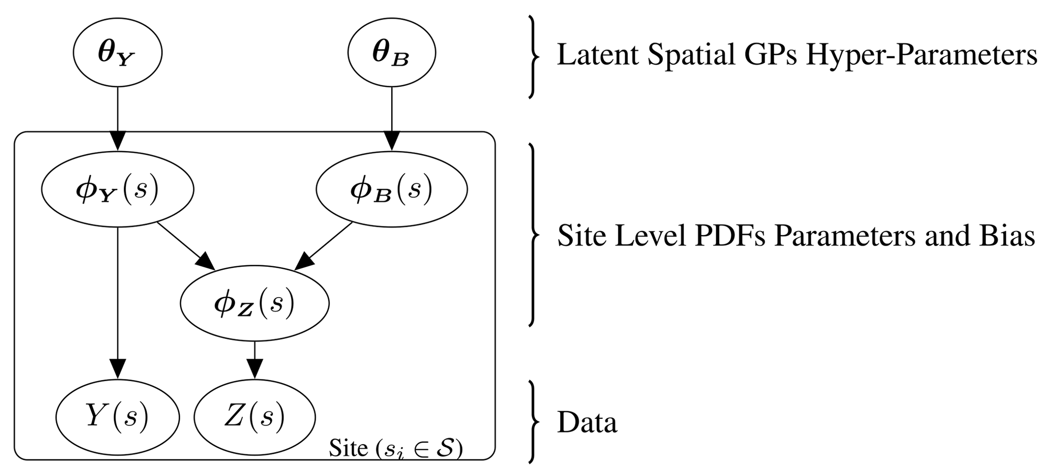
Figure 1Plate diagram illustrating the full hierarchical model. The random variables for the in situ observations, Y(s), and climate model output, Z(s), have PDFs with the collection of parameters ϕY(s) and ϕZ(s) respectively, where ϕZ(s) is modelled as the sum of ϕY(s) and some independent bias ϕB(s). The parameter ϕY(s) and the corresponding bias ϕB(s) are each themselves modelled over the domain as generated from Gaussian processes with hyper-parameters θY and θB.
Inference on the parameters of the hierarchical model given the data are applied in a Bayesian framework, where parameters of the model are themselves treated as random variables with distributions. The distribution prior to conditioning on any data is known as the prior distribution and allows for the incorporation of a domain-specific expert's knowledge in the estimates of the parameters. The updated distribution after conditioning on the observed data is known as the posterior and is approximated using Markov chain Monte Carlo (MCMC) methods, which provide samples of the parameters from the distribution . Estimates of the parameters ϕY and ϕZ at any set of new locations can then be made by constructing the posterior predictive distribution; in particular, for the purpose of bias correction, estimates of ϕY at the climate model locations can be made by sampling from the posterior predictive distribution of .
After obtaining multiple realisations of ϕY(sz) and ϕZ(sz), quantile mapping is then used to bias-correct the climate model time series at every grid cell location. Specifically, for each value of the time series from the climate model output at a given point (), this involves finding the percentile of that value using the parameter and then mapping the value onto the corresponding value of the equivalent percentile of the PDF estimated for the unbiased process, defined through the parameter . The cumulative density function (CDF) returns the percentile of a given value and the inverse CDF returns the value that corresponds to a given percentile, which results in the correction function , where F represents the CDF at a specific site. The CDF can be estimated as an integral over the parametric form assumed for the PDF. The Bayesian hierarchical model presented provides a collection of realisations for ϕY(sz) and ϕZ(sz) from an underlying latent distribution. Applying quantile mapping with each set of realisations then results in a collection of bias-corrected time series, with an expectation and uncertainty. The full framework for bias correction proposed in this paper is then illustrated in Fig. 2. The formulation for the posterior and posterior predictive is given in Appendix C.
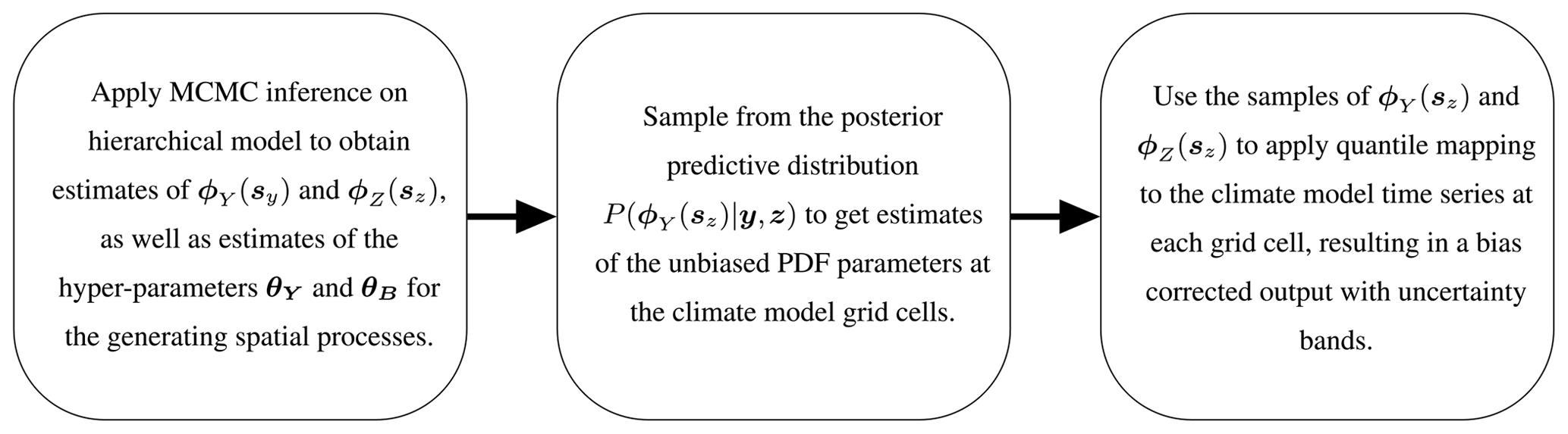
Figure 2The full bias correction framework proposed in this paper, broken down into the key steps.
The goal of the hierarchical model in Fig. 1 is primarily to estimate, with reliable uncertainties, the true unbiased values of the PDF parameters at each location of the climate model output so bias correction can be applied. Simulated examples are generated that highlight the advantage of two key features of the methodology over other approaches in the literature: modelling shared spatial covariance between the in situ data and climate model output through the inclusion of a shared generating latent process (Sect. 3.1) and the Bayesian hierarchical framework with uncertainty propagation (Sect. 3.2). One-dimensional simulated examples are chosen for clarity when illustrating these features, although it is noted that the implementation works for higher-dimensional domains, as is useful in real-world scenarios.
3.1 Non-hierarchical examples: data generation
To illustrate the potential advantage of modelling shared generating spatial processes, non-hierarchical examples are generated for simplicity. Direct measurements are assumed for one parameter of the PDFs for the in situ observations, ϕY(sy), and for the climate model output, ϕZ(sz). The goal is to predict the unbiased parameter at the climate model location ϕY(sz) using information from both sets of input data, ϕY(sy) and ϕZ(sz), which are related by . Comparison is made to the approach of inferring ϕY(sz) from the in situ data, ϕY(sy), alone, as in Lima et al. (2021). Relative performance is evaluated for three alternative simulated scenarios that correspond to different possible real-world situations. The data are generated assuming the model in Fig. 1, where the GPs are taken with constant mean, and a radial basis function (RBF) kernel, with constant kernel length scale and kernel variance. The specific values of the hyper-parameters used to generate the data and the number of observations under the different scenarios is given in Table 1.
For each scenario, a sample of the parameters ϕY(s⋆) and ϕB(s⋆) is taken from the distributions and at regularly spaced high-resolution intervals. These samples are referred to here as complete realisations and represent underlying fields for each parameter across the domain. The complete realisations of ϕY(s⋆) are sampled at lower-resolution randomised locations, with the addition of some noise, to provide direct simulated “in situ observations” of the parameter ϕY(sy). In order to simulate input data for the parameter ϕZ(sz) of the climate model output, the complete realisations of ϕY(s⋆) and ϕB(s⋆) are sampled at regularly spaced intervals to provide ϕY(sz) and ϕB(sz), and then the sum of these samples at each location is taken to give ϕZ(sz). The input data for inference are then ϕY(sy) and ϕZ(sz) and can be considered the training set, while the underlying realisations generated for ϕY(sz) are the test set used for validating the model performance.
Data are generated for three scenarios chosen to represent different potential real-world situations, illustrated in Fig. 3. The first scenario (Fig. 3a) represents an example case where it is expected that there are ample data provided in the form of in situ observations to capture the features of the underlying complete realisation of ϕY without significant added value provided from the inclusion of the climate model output during inference. The second scenario (Fig. 3b) is an adjustment where the in situ observations are relatively sparse and the underlying bias is relatively smooth. In this situation, the climate model output should provide significant added value in estimating ϕY across the domain since it is only afflicted by a comparatively simple bias that is easy to estimate. The final scenario (Fig. 3c) also involves sparse in situ observational data but with a reduced smoothness of the bias compared to the other scenarios. In this scenario, the climate model output should provide added value in estimating ϕY across the domain, but this will be limited compared to scenario 2 due to the difficulty of disaggregating the components and estimating the comparatively more complex bias.
In practice, real-world data sets are likely to be a combination of these scenarios. For example, the methodology in Lima et al. (2021) is applied to bias correcting precipitation over a domain covering South Korea and the surrounding ocean. Over land, there is a sufficient spatial density of observational rainfall gauges to adequately capture the spatial features of the unbiased underlying field from the observations alone (similarly to scenario 1). Over the ocean, rainfall gauges are very sparse and so its important to consider the spatial patterns observed from the climate model output (similarly to scenario 2). Not accounting for the spatial features seen in the climate model output over the ocean results in undesirable extrapolation over this region, as seen in the results presented in Lima et al. (2021). This undesirable property is something that is addressed by the methodology proposed in this paper, as illustrated by results for scenario 2 given in Sect. 4.1.
Table 1A table showing the hyper-parameters of the two latent Gaussian processes used to generate the complete underlying realisations of ϕY(s⋆); ϕB(s⋆); and, hence, ϕZ(s⋆), as well as observations of ϕY(sy) and ϕZ(sz), on which inference is done for three scenarios. The number of observations representing in situ data and climate model output is also given.
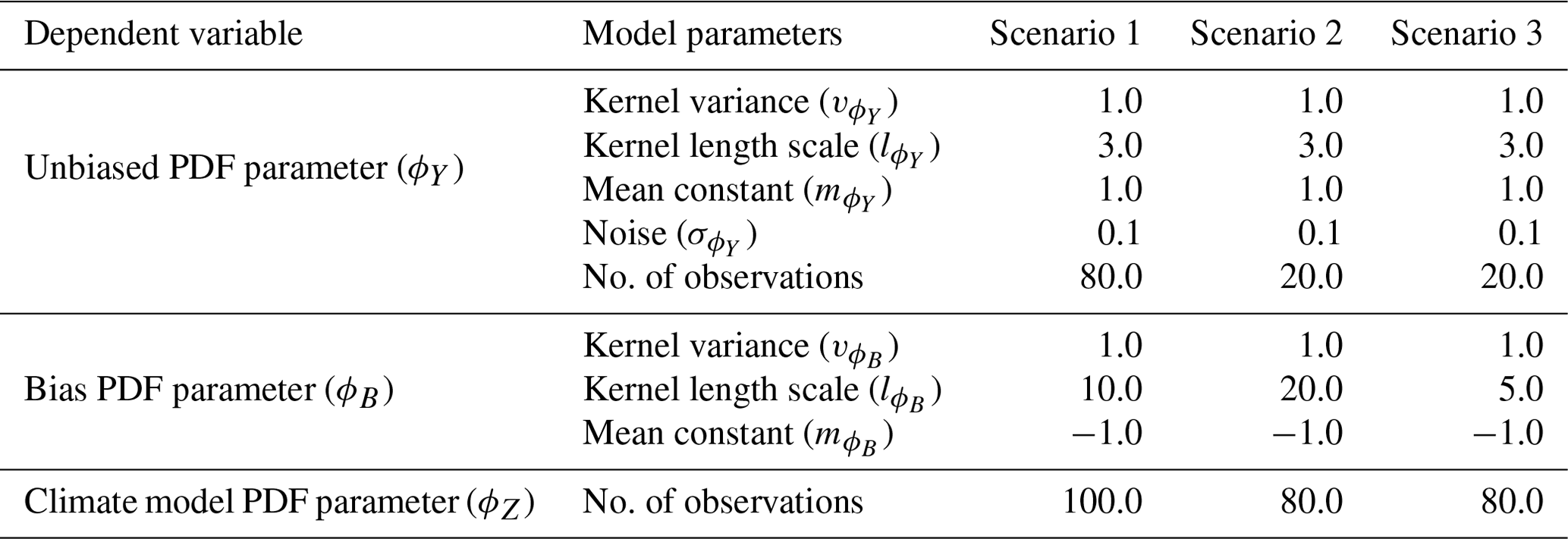
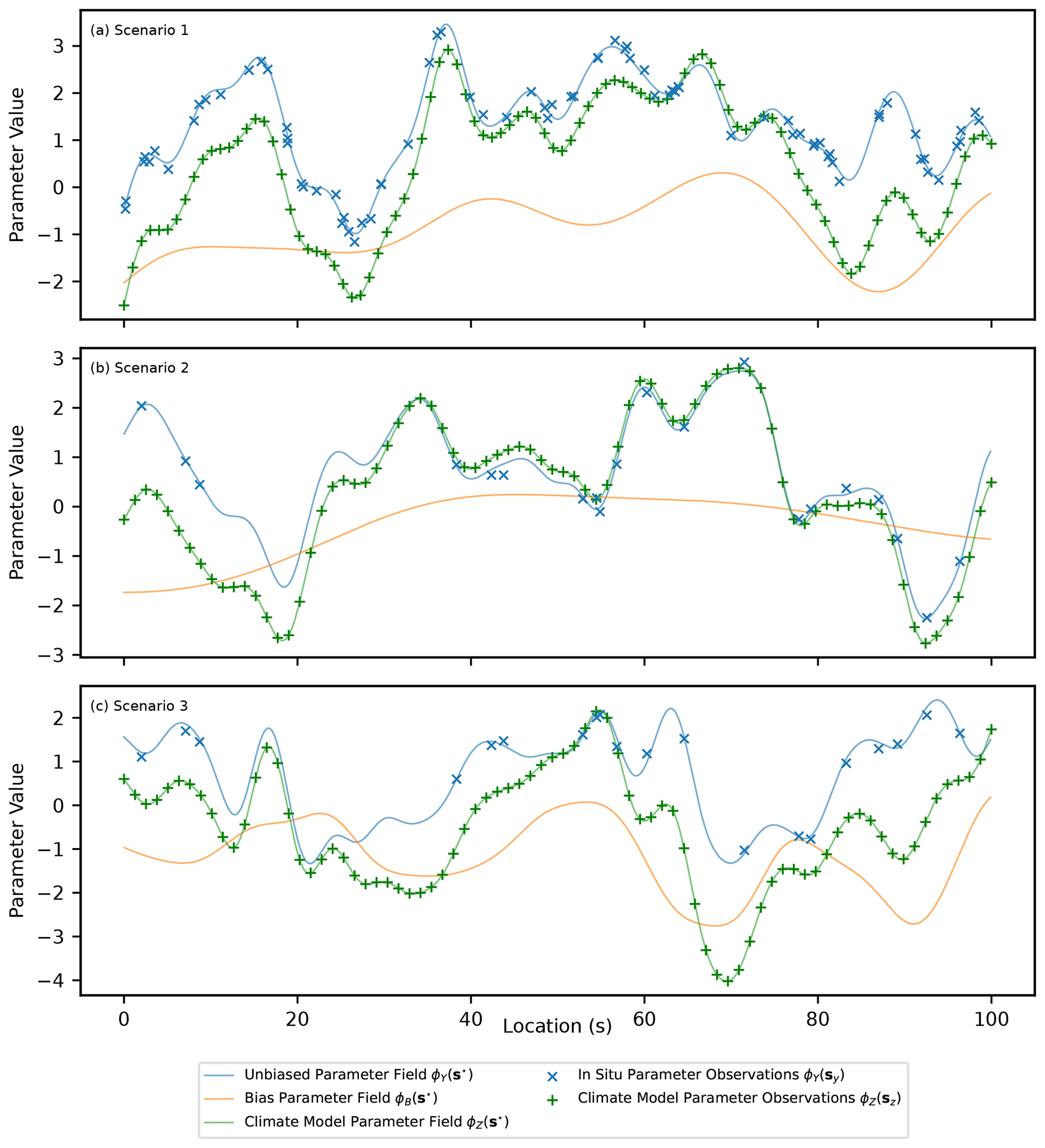
Figure 3A figure showing simulated observed data for the PDF parameters ϕY(sy) and ϕZ(sz), as well as the underlying complete realisations for each parameter and the underlying bias (ϕY(s⋆), ϕZ(s⋆) and ϕB(s⋆)). Three scenarios are shown and correspond to data generated from parameters in Table 1.
3.2 Hierarchical example: data generation
Following on from the non-hierarchical examples, to illustrate the advantage of uncertainty propagation in the Bayesian framework, a hierarchical example is generated. In situ data and climate model output are simulated at each site as generated from normal distributions such that and , as in Appendix D. The relationship is assumed for the mean parameters, where μB(s) is the bias of the mean for the climate data. For the standard deviation, the parameters are first transformed using a logarithmic link function, and then the relationship is assumed, where is the bias in the transformed parameter. The latent distributions that generate μY(s), μB(s), and across the domain are assumed to be independent GPs with a constant mean and an RBF kernel. The hyper-parameters for these latent generating processes are set for a single scenario, as given in Table 2 along with the number of simulated observation locations and the number of samples per location. A sample of the parameters μY(s⋆), μB(s⋆), and is taken from the distributions , , and at regularly spaced high-resolution intervals. These samples are referred to as complete realisations and represent the underlying fields for each PDF parameter across the domain. The complete realisations of μY(s⋆) and are sampled at a selection of lower-resolution randomised locations that represent simulated in situ observation sites to give μY(sy) and . Multiple observations of Y(si) are then generated at each in situ observation site by sampling from the corresponding normal distribution, . In the case of the simulated climate model output, samples are first taken from μY(s⋆), μB(s⋆), and at regularly spaced intervals, then the sum of these samples at each location is taken to give μZ(sz) and . The climate model output is then generated at each of these locations from the corresponding normal distribution, .
In the generated example, there are 40 locations corresponding to simulated in situ observation sites, where, for each site, 20 measurements are generated. There are 80 locations corresponding to simulated climate model output grid points, and, at each location, 100 samples are generated. This reflects the typical scenario, where the climate model output has greater spatiotemporal coverage than in situ observations but is afflicted with bias. In Fig. 4, examples of the generated samples of Y(si) and Z(si) are shown that correspond to the nearest sites for three locations. It is clear that, due to limited observations, there will be significant uncertainty in estimates of the mean and standard deviation parameters at each site and it is important that this uncertainty be propagated to the inference of the hyper-parameters for the latent GPs and also to the estimates of the unbiased PDF parameters at the climate model locations (μY(sz) and ). The underlying complete realisations of the parameters μY(s⋆), μZ(s⋆), σY(s⋆) and σZ(s⋆), as well as the bias, μB(s⋆) and σB(s⋆), are shown in Fig. 5. In addition, the empirical mean value and standard deviation of the generated data are illustrated at the simulated in situ observation and climate model sites. The goal of the hierarchical model is then to predict the unbiased values for the parameters of the PDFs at the locations of the climate model output (μY(sz) and ) while propagating uncertainty. An example of how the uncertainty in predictions of μY(sz) and is propagated through quantile mapping is then provided.
Table 2A table showing the hyper-parameters used to generate the complete underlying realisations and the measurement data on which inference is done for the hierarchical scenario. The number of sites where data are generated along with the number of samples for each site is also given.
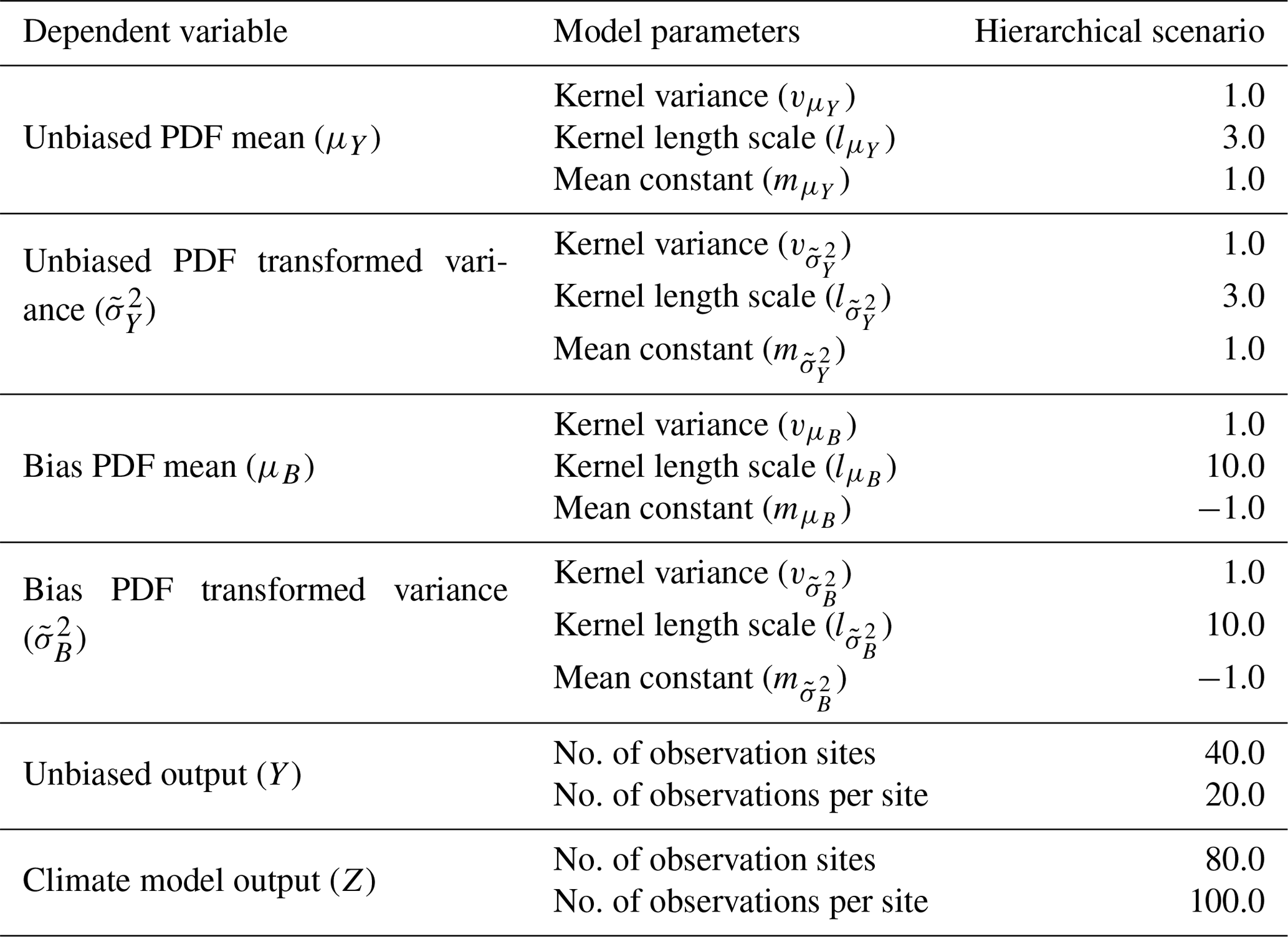
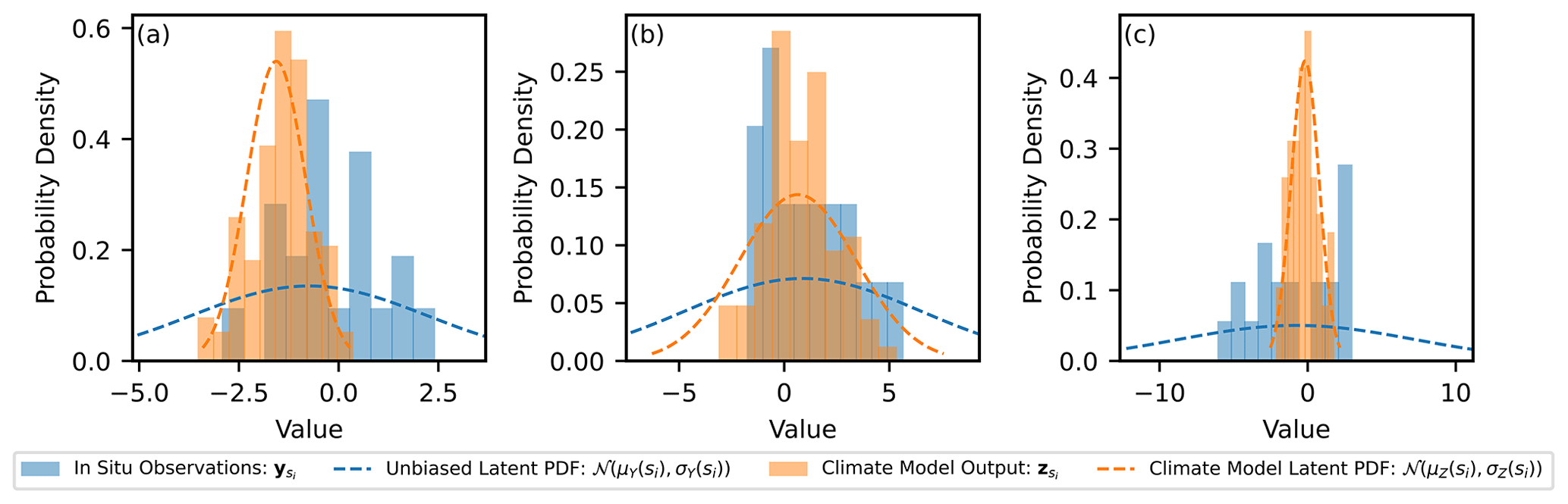
Figure 4Histograms for the climate model output at three locations and the corresponding data from the nearest in situ observation site. The locations are (a) s=11.4, (b) s=46.8 and (c) s=79.7. The latent normal distribution the data is generated from is illustrated as a dashed line.
Figure 5Simulated complete realisations for the parameters μY(s⋆), μB(s⋆), μZ(s⋆), , and , as well as the empirical values at the observation locations for the in situ and climate model data.
Inference is done in a Bayesian framework using MCMC and the No-U-Turn Sampler (NUTS) algorithm (Hoffman and Gelman, 2014) implemented in NumPyro (Phan et al., 2019). For the MCMC sampling, 1000 iterations were used for warm-up, and then 2000 samples were taken, which was found to be adequate for convergence. The parameters and hyper-parameters are treated as random variables with associated probability distributions. A prior distribution is set for each hyper-parameter and represents the belief in the distribution before observing any data, which typically incorporates knowledge from application-specific experts. In the examples presented, relatively non-informative priors are chosen since the data are simulated and represent generic examples. The posterior distribution of each parameter and hyper-parameter is the updated distribution after observing and conditioning on the data. Estimates of the PDF parameters, and , and the corresponding bias, , at new locations away from the observation sites are then referred to as samples from the posterior predictive distribution.
4.1 Non-hierarchical examples: results
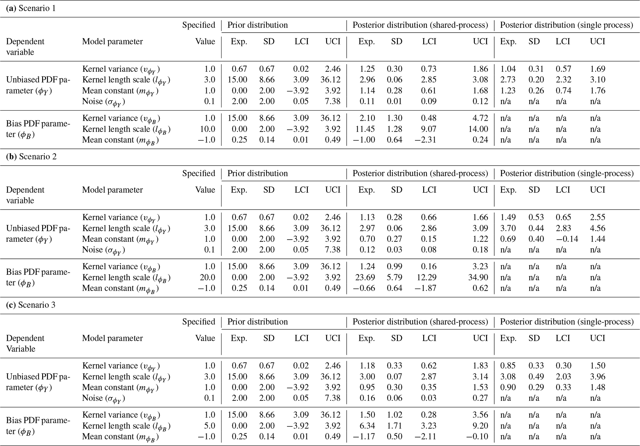
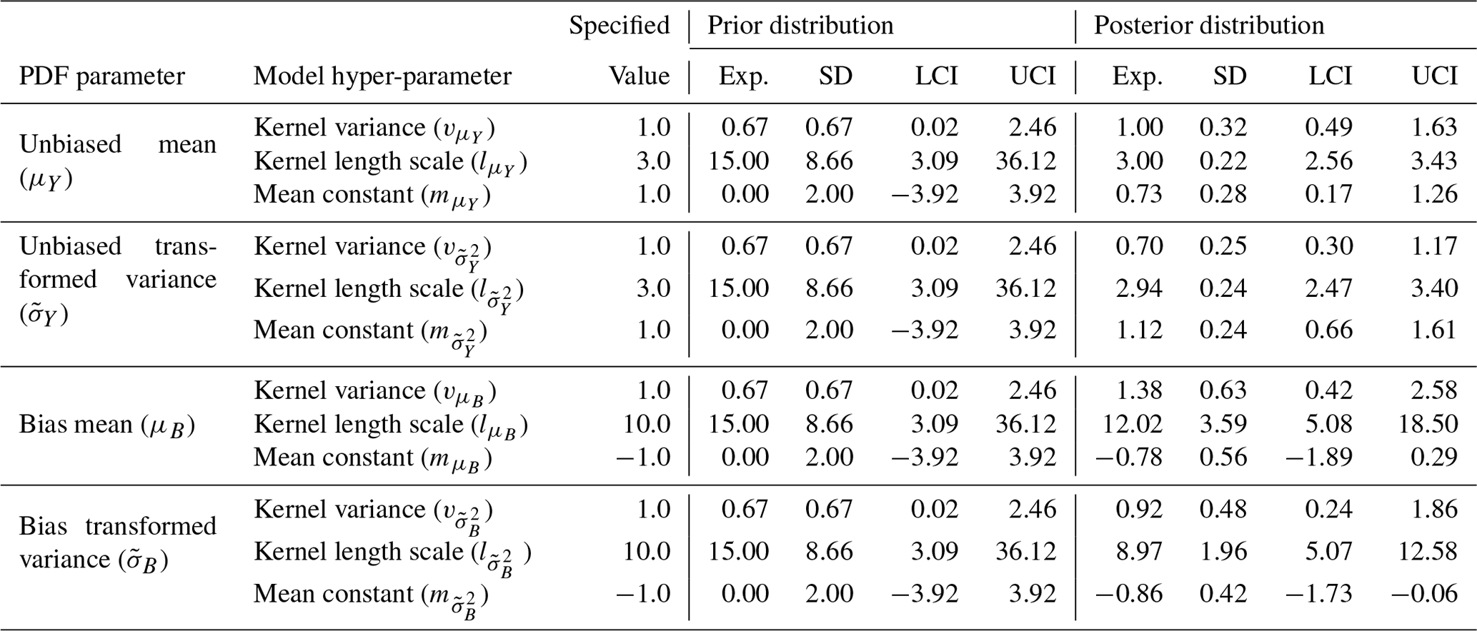
The shared latent process model presented in this paper is fit to the three non-hierarchical example scenarios, as discussed in Sect. 3.1. Input data for ϕY(sy) and ϕZ(sz) are provided and the hyper-parameters for the latent GPs that generate the unbiased and biased components inferred. Comparisons between the estimates of the hyper-parameters for the unbiased process (, and ) are made as part of the approach of only fitting to the in situ data, referred to here as the single-process approach since the latent process generating the bias is not modelled. The difference between the shared- and single-process approaches is detailed further in Appendix E. The expectation, standard deviation and 95 % credible intervals for the prior and posterior distributions of the hyper-parameters under the three different scenarios are given in Table 3. Illustrations of the prior and posterior distributions for each hyper-parameter are plotted in Fig. F1 in Appendix F.
Under all scenarios, the 95 % credible interval of the posterior for every hyper-parameter bounds the value specified when generating the data. The expectation for the posterior distribution of the unbiased hyper-parameters is, in general, closer to the specified value in the shared-process model compared with the single-process model, and the range of the credible interval is smaller. In scenarios 1 and 3, the differences between the shared- and single-process model posteriors are relatively insignificant for the mean constant () and kernel variance (), although the shared-process model shows a noticeable reduction in the uncertainty in the kernel length scale (). In scenario 2, the difference is more significant, and clear improvement is shown for the shared-process model in both the expectation and the uncertainty in hyper-parameter estimates.
Table 3A table showing summary statistics for the prior and posterior distributions including the expectation (Exp.), standard deviation (SD) and lower and upper bounds for the 95 % credible interval (LCI and UCI respectively). The posterior distributions for the shared- and single-process models are given. The specified value for each parameter used to generate the data is also shown. In the single process model the bias parameters and the noise are not modelled and so labelled as not applicable (“n/a”).
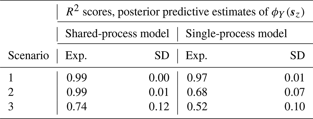
After applying MCMC inference to the parameters and hyper-parameters that generate the data, posterior predictive estimates are made for the unbiased PDF parameter values at the simulated locations of the climate model (ϕY(sz)). These estimates are presented in Fig. 6 for each scenario and for both the shared-process and the single-process models. Additionally, estimates of the underlying bias, ϕB(s), are shown for the shared-process model, since the bias is explicitly modelled. The relative performance of the shared- and single-process models is quantified by computing R2 scores between the predictions of ϕY(sz) and the actual values used in generating the data (although not used in training), with results presented in Table 4. In Fig. 6, it can be seen that the predictions of ϕY(sz) in the shared-process case (Fig. 6d, e and f) are closer to the true underlying field and have a smaller but still realistic uncertainty compared to the single-process model. In scenario 1, the difference between the posterior predictive distributions for ϕY(sz) between the two approaches is not substantial, with both models performing adequately, having R2 scores of 0.99 and 0.97 respectively. In scenario 2, the difference between estimates of ϕY(sz) between the models is significant, with R2 scores of 0.99 and 0.68 for the shared- and single-process models respectively. Finally, in scenario 3, the difference is again significant, with R2 scores of 0.74 and 0.52 respectively, although it is less significant compared with scenario 2.
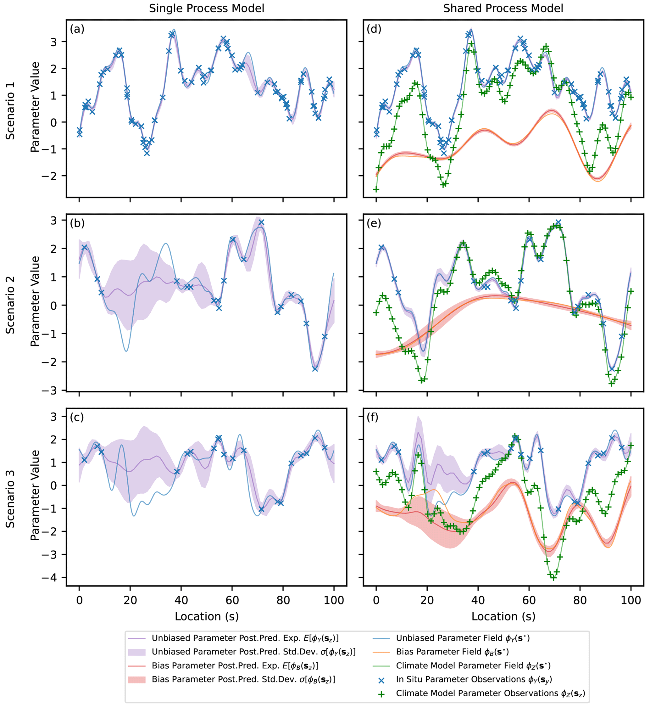
Figure 6Expectation and 1σ uncertainty in the posterior predictive distributions of the parameter ϕY(sz) and the corresponding bias ϕB(sz) for three scenarios. The underlying functions (complete realisations) as well as the simulated input data are also shown.
Table 4A table showing the expectation and standard deviation of R2 scores for the posterior predictive estimates of the unbiased PDF parameter at the climate model output locations ϕY(sz) for the shared- and single-process models for each scenario.
4.2 Hierarchical example
The hierarchical model presented in this paper is fit to the hierarchical example from Sect. 3.2. The expectation, standard deviation and 95 % credible intervals for the prior and posterior distributions of each hyper-parameter of the latent generating processes are given in Table 5. The 95 % credible interval of the posterior for every hyper-parameter bounds the value specified when generating the data. As expected, the posterior distribution for each hyper-parameter is concentrated more closely to the value specified when generating the data than the relatively non-informative prior distributions. The prior and posterior distributions for each hyper-parameter are plotted in Fig. F2 in Appendix F.
Table 5A table showing summary statistics for the prior and posterior distributions including the expectation (Exp.), standard deviation (SD) and lower and upper bounds for the 95 % credible interval (LCI and UCI). The specified value for each hyper-parameter used to generate the data is also shown.
After fitting the model, posterior predictive estimates are made using the unbiased mean and standard deviation parameters at the simulated locations of the climate model (μY(sz) and σY(sz)). Additionally, estimates of the bias in the parameters are made (μB(sz) and σB(sz)). These estimates, along with the true underlying values, are shown in Fig. 7. The empirical mean and standard deviation of the input data are also given at the locations where they are sampled. The estimates visually appear to perform well at capturing the spatial features of the underlying fields and at estimating a 1σ uncertainty range. For example, in the range of , where the main data source is the biased climate model output, the prediction accurately captures the spatial features of the unbiased parameters (μY(s) and σY(s)) with an uncertainty that bounds the true underlying value over most of the region. Additionally, uncertainty in the unbiased parameters at the in situ observation sites (μY(sy) and σY(sy)) due to limited samples is clearly reflected in the estimates.
Quantile mapping is applied to the climate model output for a single site (), and the bias-corrected time series () is shown in Fig. 8. The site chosen is at s=11.4 and is the same as in Fig. 4a. A generic time series for the climate model output and nearest in situ observations is generated from the correct mean and standard deviations of the samples. Quantile mapping is performed for each posterior predictive realisation of μY(si), μZ(si), σY(si) and σZ(si). This results in multiple realisations of bias-corrected time series with an expectation and uncertainty.
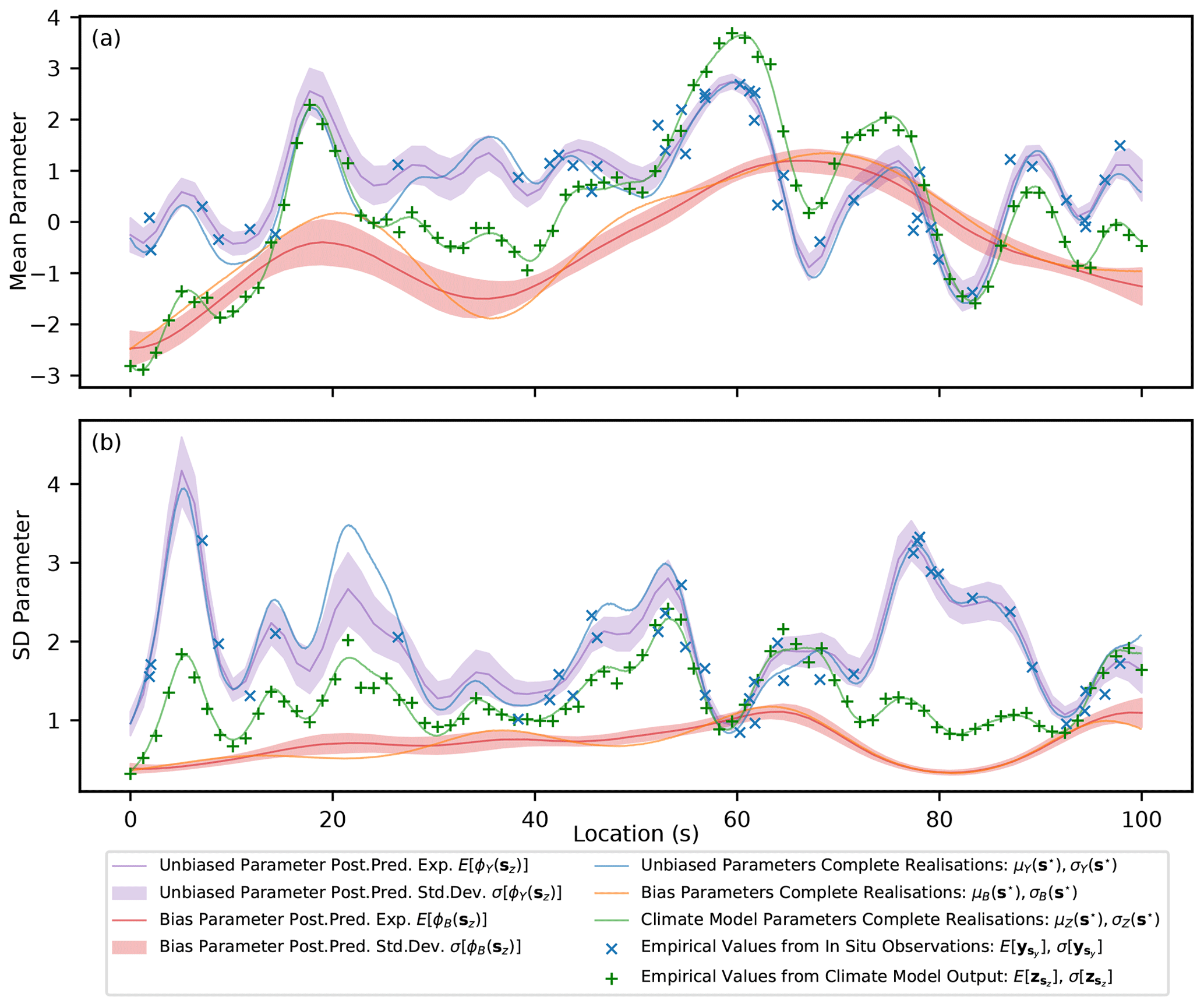
Figure 7A figure showing the expectation and 1σ uncertainty in the posterior predictive distribution across the domain for the parameters μY(sz), μB(sz), σY(sz) and σB(sz), as well as the true underlying functions.
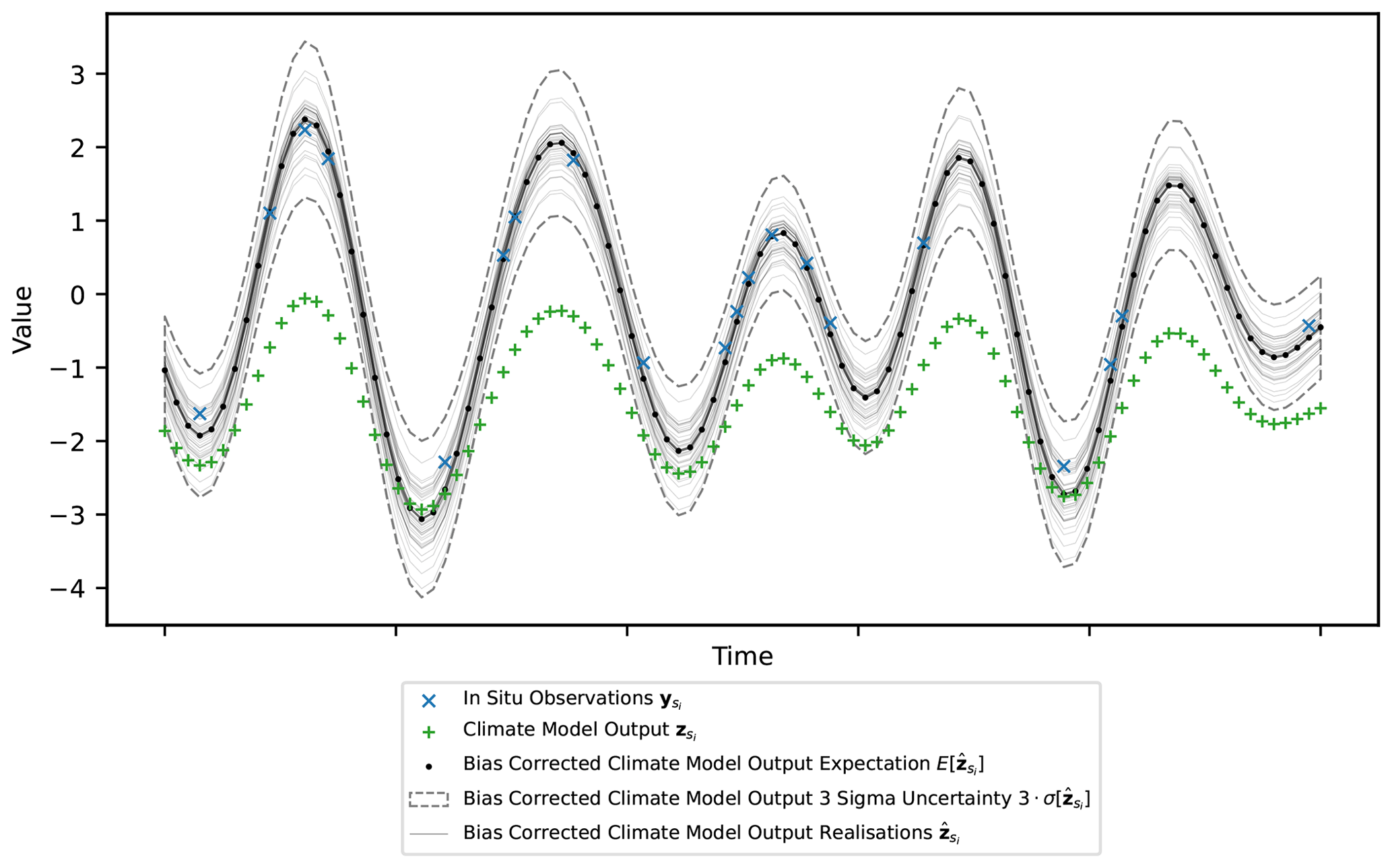
Figure 8Simulated time series for the climate model output at location s=11.4 and for the nearest in situ observation site. Realisations of the climate model bias-corrected time series are shown along with the expectation and 3σ uncertainty range.
The bias correction framework proposed in this paper models the parameters of the PDFs for the in situ observations and climate model output across the domain using a Bayesian hierarchical model. This allows for estimates to be made of the unbiased PDF parameters at the climate model locations, and quantile mapping can then be applied to bias-correct the climate model time series. The hierarchical model uses GPs to model the spatial covariance structure of the PDF parameters and assumes that each parameter of the climate model output is generated using two independent GPs: one that generates an unbiased component and another that generates a bias. The GP that generates the unbiased component is also modelled to generate the equivalent PDF parameters for the in situ data. This approach reflects the belief that the climate model provides skilful estimates of the PDF parameters across the domain and that the spatial covariance structure, generated from equations based on established physical laws, has spatial features similar to the true unbiased PDF parameter values. The climate model output, while afflicted by bias, provides comprehensive spatiotemporal coverage and useful information in the inference of the unbiased PDF parameters across the domain. This is assuming the bias signal can be adequately deconstructed from the climate model output with the use of in situ observations. In Sect. 4.1 of the results, the added value of modelling shared latent GPs between the in situ observations and climate model output is demonstrated. This is compared with the approach of modelling a latent GP for the in situ observations alone and inferring the unbiased PDF parameters without incorporating information from the climate model output, as in Lima et al. (2021), which is here referred to as the single-process approach.
The added value is assessed for three scenarios with a differing density of observations and spatial complexity of the bias signal. The methods used to assess the added value include comparisons of summary statistics for the posterior distributions of the GP hyper-parameters, visual comparisons between the expectation and standard deviation for posterior predictive estimates of the unbiased PDF parameters across the domain, and comparison of R2 scores for the unbiased PDF parameter at the locations of the climate model output. It is shown that across all these measures, the most added value is provided where the in situ observations are relatively sparse compared with the climate model output and the underlying bias is relatively spatially smooth compared with the unbiased signal, as in scenario 2. In this scenario, despite sparse in situ observations, since the bias signal varies smoothly across the domain the climate model, output can be accurately and precisely disaggregated into its unbiased and biased components. This leads to improved estimates of the unbiased PDF parameters at the climate model locations when considering shared GPs compared with the single-process approach that uses in situ observations alone; see Fig. 6.
As the density of in situ observations is increased to levels similar to the climate model output itself, the value added from the climate model output in inference of the unbiased parameters is reduced, which is illustrated by results for scenario 1. The number of in situ observations is sufficient to adequately capture the spatial features of the underlying process (Fig. 6a) as well as the latent spatial covariance structure, encoded through the hyper-parameter estimates of the latent GP (Table 3). Additionally, as the complexity of the bias signal is increased by, for example, reducing the length scale of the latent generating process, as in scenario 3, the added value is again reduced. The relatively more complex bias structure compared with scenario 2 makes it more difficult to disaggregate the climate model output into its biased and unbiased components. Despite this, while added value is reduced for scenarios 1 and 3 relative to scenario 2, incorporating the climate model output in inference is still shown to improve overall performance. Modelling the generating process for the bias also explicitly provides informative information that is potentially useful for future climate model development.
In addition to modelling shared latent processes, another important feature of the methodology presented in this paper is the Bayesian framework. In this framework, the parameters and hyper-parameters of the hierarchical model are treated as random variables with associated probability distributions. Uncertainty is inherently propagated through the framework, making the code implementation flexible regarding further development and therefore applicable to a wide range of real-world scenarios. Additionally, a Bayesian framework allows for expert knowledge to be incorporated in the inference through the choice of prior distributions, which can be especially important where the data are sparse. In Sect. 4.2, results for a simulated hierarchical example illustrate uncertainty propagation between the PDF parameter values and the hyper-parameters of the latent generating processes. Uncertainty present in the different levels of the hierarchical model is incorporated in the final posterior predictive estimates of the unbiased PDF parameters at the climate model locations; see Fig. 7. Multiple realisations from the posterior predictive can then be used in quantile mapping to produce multiple realisations of the final bias-corrected time series with an expectation and uncertainty range, as illustrated in Fig. 8. Reliable uncertainty bands in the final bias-corrected time series are important for impact assessments and resulting decision-making. Additionally, having multiple realisations of the final bias-corrected time series allows for further propagation of uncertainty in process models driven by climate model output, such as land surface models (Liu et al., 2014).
The simulated examples presented provide an initial proof of concept, although future studies validating the methodology against real-world applications are important for understanding the remaining limitations and areas for further development. The current primary limitation is expected to be that the underlying spatial covariance structures are assumed to be stationary – that is, that the covariance length scale is assumed to be constant across the domain – whereas for real-world applications over large and complex topographic domains, the length scale is expected to change depending on the specific topography of the region. Further development of the methodology to incorporate non-stationary kernels would therefore be valuable, although this is beyond the scope of this paper. Another important limitation to consider is the assumption that the bias is time-independent. In situations where the bias varies gradually through time and uniformly across the domain, the methodology can be further developed such that the mean function of the GPs is modelled with a time dependency. If the bias varies in time non-uniformly across the domain, spatiotemporal GPs will need to be considered, which is again beyond the scope of this paper. Secondary limitations include the assumption that the unbiased and biased components of the PDF parameter values are independent. In situations where there is a dependence between these components, the methodology presented is still expected to perform adequately, although information is lost by not modelling the dependency explicitly. Additionally, many real-world applications will necessitate specific model adjustments, such as incorporating a mean function dependent on factors like elevation and latitude. Finally, the computational complexity of the model is an important remaining consideration, with inference time of GPs being the cube of the number of data points. Incorporating techniques from the literature, such as using sparse variational GPs (SVGPs) (Hensman et al., 2015), using nearest-neighbour GPs (NNGPs) (Datta et al., 2016) or upscaling the climate model output, while outside the scope of this paper, will aid computational performance under demanding real-world scenarios and will facilitate further model development.
Current approaches to bias prediction and correction do not aim to preserve the spatial covariance structure of the climate model output and typically either neglect uncertainty or inadequately model uncertainty propagation (Ehret et al., 2012). This paper presents a novel fully Bayesian hierarchical framework for bias correction with uncertainty propagation and latent GP distributions used to capture and preserve underlying covariance structures. In this framework, bias is considered in the parameters of the time-independent PDF at each site. Estimates of the unbiased PDF parameters are made at the climate model locations, and quantile mapping is then applied to produce the final bias-corrected time series. The novelty of the approach lies in the fully Bayesian implementation, assuming shared latent GPs between the in situ data and climate model output and in propagating uncertainty through the quantile mapping step. Simple simulated examples are chosen to illustrate key features of the framework. In Sect. 4.1, results are displayed for non-hierarchical examples where the focus is on illustrating the advantage of modelling spatial covariance in both in situ data and climate model output, assuming shared latent GPs. This is shown to be particularly important in the case of sparse in situ observations and bias that varies smoothly across the domain, where the climate model output itself provides significant added value in predictions of the unbiased PDF parameters. In Sect. 4.2, results are presented for a hierarchical case and focus is on illustrating how the model propagates uncertainty between the different levels and to the final unbiased PDF parameter predictions at the climate model locations. In addition, a simulated example of propagating this uncertainty through quantile mapping is then provided to demonstrate how this results in a bias-corrected time series with uncertainty bands, which is desirable for use in impact studies and for informing decision-making. Adequately modelling uncertainty in the bias-corrected time series is expected to be especially important over areas where the climatology is hard to model and in situ observations are sparse, such as over Antarctica (Carter et al., 2022). The framework presented provides a step towards adequately capturing uncertainty and incorporating underlying spatial covariance structures from the climate model in bias correction. While initial results are promising, further studies applied to real-world data sets are important to further validate the approach and explore remaining limitations. The Bayesian implementation provides a flexible modelling framework, where adjustments to the methodology needed for specific applications can be made while inherently propagating uncertainty.
Bias in climate models is defined in a number of similar ways across different papers. In Maraun (2016), it is defined as the systematic difference between any statistic derived from the climate model and the real-world true value of that statistic, while in Haerter et al. (2011), bias is defined as the time-independent part of the error between the climate model simulated values and the observed values. In general, across the community involved with climate change impact studies, bias is used to refer to any deviation of interest between the model output and that of the true value (Ehret et al., 2012). Deviations of interest are typically with respect to the statistical properties of the data – for example, the mean and variance – as well as spatial properties, such as the covariance length scale. The methodology developed in this paper treats bias with respect to deviations in the PDFs of the climate model output and observations at each site. Assuming a parametric form for the PDF, this translates to evaluating bias of the parameters of the site-level PDFs, as discussed in Sect. A1. In order to model bias in real-world phenomena while considering the intrinsic spatial structure, the parameters are allowed to vary spatially using stochastic processes; see Sect. A2. After evaluating bias across the domain, the methodology in this paper can be combined with current approaches to correcting bias in climate models, such as quantile mapping, which are discussed further in Sect. A3.
A1 Bias in random variables
Consider a specific in situ observation site (e.g. an automatic weather station) with measurements of some variable , such as midday temperature, and also comprehensive predictions from a climate model at the same location, . In this scenario, bias can be defined in terms of discrepancy between the PDFs of the in situ observations and the climate model predictions. In particular, assuming a parametric density function for both random variables, bias is translated to the discrepancy between the parameters of the PDFs. For example, assuming the observation measurements are independent and identically distributed (i.i.d.) with normal distribution and the equivalent for the climate model outcomes, , bias can then be quantified by some discrepancy function of the mean parameters, μZ and μY and the standard deviations, σZ and σY. This function can be defined in different ways – for example, as the difference or the ratio .
A2 Bias with spatially varying parameters
Real-world applications, such as impact studies, typically require bias to be evaluated over a spatial region rather than just at a point. Consider a collection of n observational sites, , where for each site i there exist m daily measurements of some property, such as midday temperature, . In addition, consider gridded output from a climate model of the same property at a set of different locations, s*. In this scenario, instead of defining bias in terms of the discrepancy in the PDFs at a single point, bias can be defined with respect to the two latent spatial processes underlying the observed data, {Y(s)}, and the climate model output, {Z(s)}. This allows for bias to be estimated across the domain.
As an example, assume that observations and the climate model output come from the spatial stochastic processes and respectively, where the distribution of data at each location s is normal, with spatially varying parameters μ(s) and σ(s). The spatial structures of the latent processes are inherited from the spatial structures in the parameters, which are themselves modelled throughout the domain as spatial stochastic processes {μY(s)}, {σY(s)}, {μZ(s)} and {σZ(s)}. In this paper, GPs are used to model the spatial structures, which explicitly capture relationships for the expectation and covariance between points across the domain; see Appendix B. Bias is then defined by some discrepancy function of these spatially varying parameters, such as .
A3 Bias correction
Bias correction involves using observational data to predict and then reduce bias in the climate model output, with techniques varying in focus and complexity. For example, the delta change method aims to simply apply an adjustment to the mean of the variable under study at each location (Das et al., 2022), while quantile mapping aims to correct the whole PDF of the climate model output (Qian and Chang, 2021). In Beyer et al. (2020), generalised additive models (GAMs) are used to approximate transfer functions between the climate data and the observed values. The relative performance between methods is assessed in various studies (Teutschbein and Seibert, 2012; Räty et al., 2014; Beyer et al., 2020; Mendez et al., 2020). Different approaches typically fail to adequately capture uncertainty and to explicitly model spatial dependencies between locations across the domain. The approach proposed in this paper combines the use of a Bayesian hierarchical model for predicting bias across the region with the established approach of quantile mapping for applying the final correction to the climate model output. Uncertainty is propagated through the framework, and underlying spatial structures are explicitly modelled using latent spatial stochastic processes.
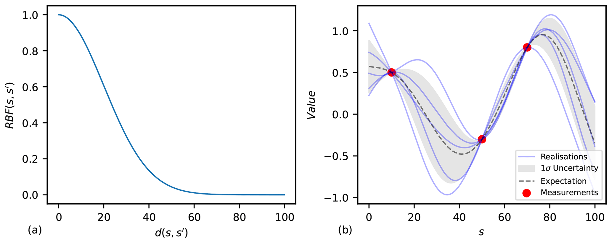
Figure B1(a) Values of the RBF function with a kernel variance equal to 1 and length scale equal to 20. (b) Realisations of the GP with the equivalent kernel as in (a) and conditioned on three data points. The expectation and uncertainty in the distribution are shown.
A collection of random variables, , indexed according to location in a domain can be modelled using a spatial stochastic process, such as (shorthand {ϕ(s)}), where 𝒮 represents the region under study. The family of Gaussian processes (Rasmussen, 2004) has the property that any finite subset of random variables across the domain is modelled as a multivariate normal (MVN) distribution. Consider a collection of k random variables; then, the joint distribution between these variables is MVN, with , where ϕ is some k-dimensional random vector, μ is some k-dimensional mean vector and Σ is some k-by-k-dimensional covariance matrix. Parameterising the mean and covariance of the MVN distribution then gives the GP, which provides a distribution over continuous functions . The collection of parameters for the mean and covariance functions is often referred to as hyper-parameters.
The mean function, m(s), of a GP gives the expectation of the parameter at the location index, allowing for global relationships for the variable given predictors. In this paper, the mean function is considered a constant across the domain for simplicity and is such that m(s)=m. In real-world applications, a more complex relationship is likely to be useful; for example, Eq. (B1) assumes a second-order polynomial in two predictors, where the predictors x1(s) and x2(s) could be elevation and latitude.
The kernel (covariance) function is typically some function of distance between points, , parameterised by a length scale, l, and kernel variance, v; for example, Eq. (B2) gives the well-known radial basis function (RBF) for the kernel. The function of distance could be Euclidean or geodesic and arbitrarily complex, including factors such as wind paths. The two-dimensional Euclidean case is given in Eq. (B3), where predictors x3(s) and x4(s) could, for example, be latitude and longitude, which, for relatively small distances near the Equator, are approximately Euclidean. In Fig. B1, an example of how the covariance decays with distance is given for the RBF kernel in panel (a), and realisations of a conditioned GP with the equivalent kernel are illustrated in panel (b).
The kernel is often assumed stationary for simplicity, as in Lima et al. (2021), meaning that the relationship between covariance and distance is consistent across the domain of study. This assumption is used in the simulated results presented in this paper. The validity of the stationarity assumption should be assessed on an application basis, with factors such as complex topography contributing to non-stationarity.
Gaussian processes have the property that the sum of independent GPs is also a GP. This property is utilised in this paper as the additive relationship is assumed, where ϕY and the bias, ϕB, are taken to be independent and generated from latent Gaussian processes. Note that in the case of different supports between the parameter space and that of the sample space of a Gaussian process, a link function is then included and the relationship assumed, where the parameters and are modelled as independent and generated from GPs. Assuming an additive relationship results in an easy-to-define distribution for ϕZ (or ), which is a GP where the mean and covariances are simply the sum of the values from the independent GPs (Eqs. B4 and B5). The additive relationship captures the belief that the climate model output has some shared latent spatial covariance structure with the in situ observations but is inflicted by an independent bias. In order to make predictions from the unbiased process across the domain , conditioning is then performed on both the observed in situ data, ϕY(sy), and the observed climate model output, ϕZ(sz).
C1 Full hierarchical model
The in situ observations and climate model output are treated as realisations of the stochastic processes {Y(s)} and {Z(s)} respectively, where the random variables for a given site are distributed as Y(s)∼f(ϕY(s)) and Z(s)∼f(ϕZ(s)). The symbols ϕY(s) and ϕZ(s) represent the collection of parameters that describe the PDF at the site. The collection of in situ observation sites is given as and the collection of climate model output locations as ; the collection of PDF parameter values for each set of locations is then written as and . Each parameter of the PDFs is modelled as generated from latent Gaussian processes, one that generates the unbiased component and one that generates the bias, such that , and . The symbols and represent the collection of hyper-parameters for the Gaussian processes. The posterior distribution for the model can then be written as
The first part of the numerator for the fraction can be broken down into
The second part of the numerator for the fraction can be broken down into
The above equations are inherently incorporated into the code implementation through the model definition using the NumPyro Python package (Phan et al., 2019). The posterior distribution is approximated using MCMC, which returns realisations of ϕY(sy), ϕZ(sz), and of the posterior. The posterior predictive estimates of, for example, , at any set of new locations across the domain, are then given by the following:
where the integrand can be broken down into
The second part of this expression is equivalent to the posterior distribution defined earlier. The realisations from the posterior provided through the MCMC inference can be used as parameter values in the first part of the expression above to give a distribution that, when sampled from, provides posterior predictive realisations for . In the case of Gaussian processes, the distribution of can be formulated in the following way, where, to start, one can take the joint distribution:
Note that since ϕY(s) and ϕB(s) are independent and applies, the covariance between the parameters ϕY(s) and ϕZ(s) is simply . Additionally, the mean and covariance terms for the process that generates ϕZ(s) are computed as and .
Then, after defining the following:
the distribution can be written as
where the conditional distribution P(U1|U2) is well known for Gaussian distributions and is given as
with parameter values
This provides the distribution P(U1|U2), which is equivalent to the distribution that is needed to compute the posterior predictive.
C2 Non-hierarchical case
In the non-hierarchical case used in Sect. 4.1, direct observations are assumed for ϕY(sy) and ϕZ(sz). In this case, the posterior for the model can be written out as
where the first expression of the numerator can be broken down into
while the second part of the numerator can be split due to independence between the generating processes as follows:
As with the full hierarchical model, the above equations are inherently incorporated into the non-hierarchical code implementation, with the posterior distribution approximated using MCMC, which returns realisations of and from the posterior. The posterior predictive estimates of, for example, at any set of new locations across the domain are then given by the following:
where the integrand can be broken down into
The second part of this expression is equivalent to the posterior distribution defined earlier. The realisations from the posterior provided through the MCMC inference can be used as parameter values in the first part of the expression above to give a distribution that, when sampled from, provides posterior predictive realisations for . The distribution in the first part of the expression can be formulated in the same way as presented in Sect. C1.
Take the case of evaluating bias in the output of near-surface temperature from a climate model relative to some in situ observations. The output from the in situ observations and the climate model are each considered realisations from latent spatiotemporal stochastic processes and respectively. To evaluate bias, the time-independent marginal distributions are taken along with the data treated as realisations from the spatial stochastic processes and . Temperature is known to have diurnal and seasonal dependency, and therefore, for the in situ observation measurements to be representative of the time-independent marginal distribution, there must be an equal spread of the data over the time of day and season. To reduce this requirement, the data can be filtered to just midday January values. Filtering the data has the added benefit of simplifying the marginal distribution and therefore also the interpretation of bias, allowing for the bias to be evaluated for different seasons individually. In the case of January midday temperature, the site-level marginal distributions can be approximated as normal, such that and .
Treating the site-level distributions as normal results in bias being defined in terms of disparities in the mean and standard deviation parameters between in situ observations and climate model output, such that and . Bias in the climate model output and the parameters of the in situ observations is considered independent and is in both cases generated by separate spatial stochastic processes. For example, the bias in the mean, μB(s), is considered independent of the mean of the in situ observations, μY(s), and both are modelled as generated by separate GPs: and . In this example, the mean function of the GP is considered a constant, and the kernel/covariance function is considered a radial basis function parameterised by kernel variance and length scale. Defining the relationship allows for taking advantage of the property that the sum of two independent GPs is itself a GP such that . See Appendix B.
In the case of the standard deviation, the parameter space () is not the same as the sample space of a GP (ℝ), and therefore, a link function is applied . The transformed parameters are then modelled as being generated from GPs: and . To again take advantage of the property that the sum of two independent GPs is itself a GP, the relationship is defined. The parameter is then distributed as . After predictions of the transformed parameter across the domain are made, the inverse link function can be applied to get estimates of the non-transformed parameter.
The diagram in Fig. D1 gives a representation of this full model in a hierarchical framework. Applying MCMC inference provides posterior realisations of the parameters of the model. This includes realisations from the posterior distribution of μY and at all in situ observation locations as well as realisations from the posterior of μZ and at all the climate model output locations. These realisations, in addition to those of the parameters from the generating GPs, can be used to compute the posterior predictive distribution of the parameters μY, , μB, , μZ and everywhere in the domain. For the purpose of applying bias correction, the posterior predictive distribution for these parameters can be evaluated at the locations of the climate model output. Quantile mapping is then applied to transform the predicted distribution of the climate model output into that of the predicted distribution for in situ observations. Applying quantile mapping or alternative methods for multiple realisations of the parameters provides an expectation and uncertainty band for the bias-corrected output.
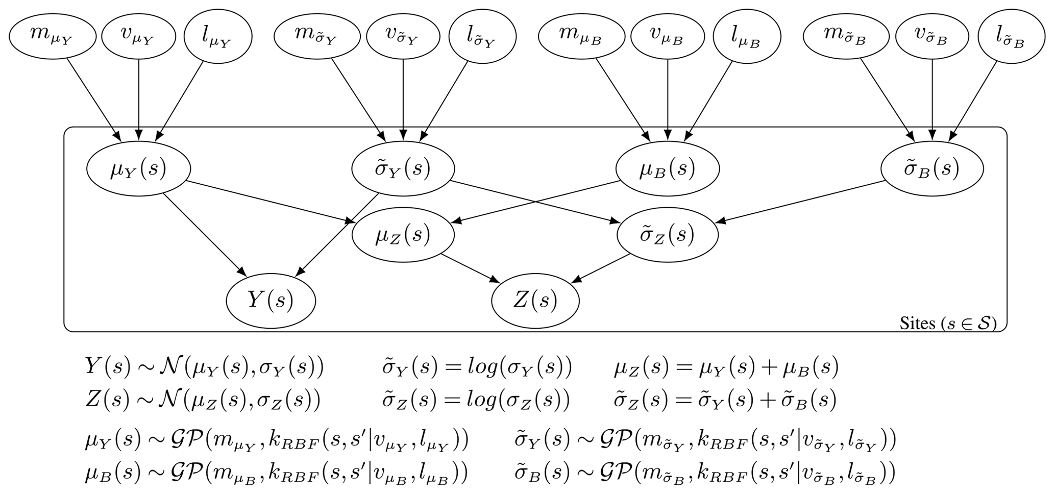
Figure D1Plate diagram with a directed acyclic graph showing the full hierarchical model for the case where the site-level distributions are assumed normal, with parameters μ and σ. The distribution of these parameters across the domain is modelled with Gaussian processes.
In the main paper, comparisons are made between the shared-process and single-process models. The shared-process model is the hierarchical model proposed in this paper, while the single-process model represents a similar approach taken from the literature; see Lima et al. (2021). The two models are shown in Fig. E1. In both models, the random variables for the in situ observations, Y(s), and climate model output, Z(s), have PDFs, with the collection of parameters being ϕY(s) and ϕZ(s) respectively. In the case of the shared-process model, ϕZ(s) is modelled as the sum of ϕY(s) and some independent bias, ϕB(s). The parameter ϕY(s) and the corresponding bias ϕB(s) are each themselves modelled over the domain as generated from Gaussian processes with hyper-parameters θY and θB. The unbiased parameter ϕY(s) and hyper-parameter θY are inferred from both in situ data and climate model output. Posterior predictive estimates of ϕY(sz) are made by conditioning on both sets of data. In the case of the single-process model, the PDF parameters for the climate model output and in situ observations are treated as independent. Only one latent GP is considered with the unbiased parameter ϕY(s) and hyper-parameter θY inferred from in situ observations alone. Posterior predictive estimates of ϕY(sz) are also made by conditioning on just in situ observations.
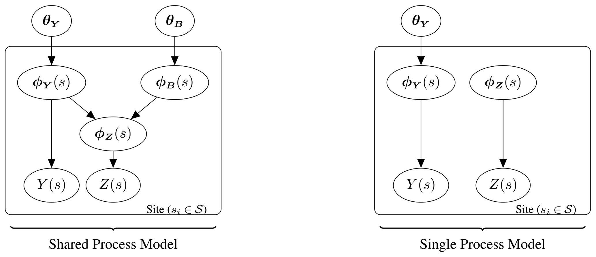
Figure E1Plate diagram illustrating the difference between the shared-process hierarchical model presented in this paper and the single-process model that comparisons are made against.
A Bayesian framework considers the parameters of the model as random variables with probability distributions. The prior is the assumed distribution before observing any data and the posterior is the updated distribution after observing data. Figures F1 and F2 illustrate the prior and posterior distributions for the non-hierarchical and hierarchical simulated examples respectively. The parameter value specified when generating the data is also shown.
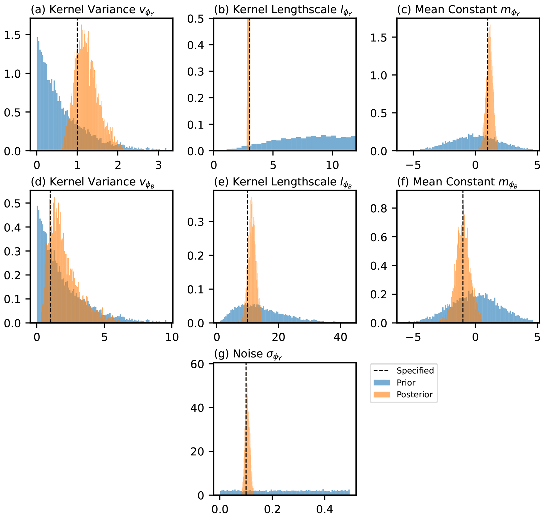
Figure F1A figure illustrating the prior and posterior distributions for the parameters of the model in the case of scenario 1. The value that was specified when generating the data is also shown.
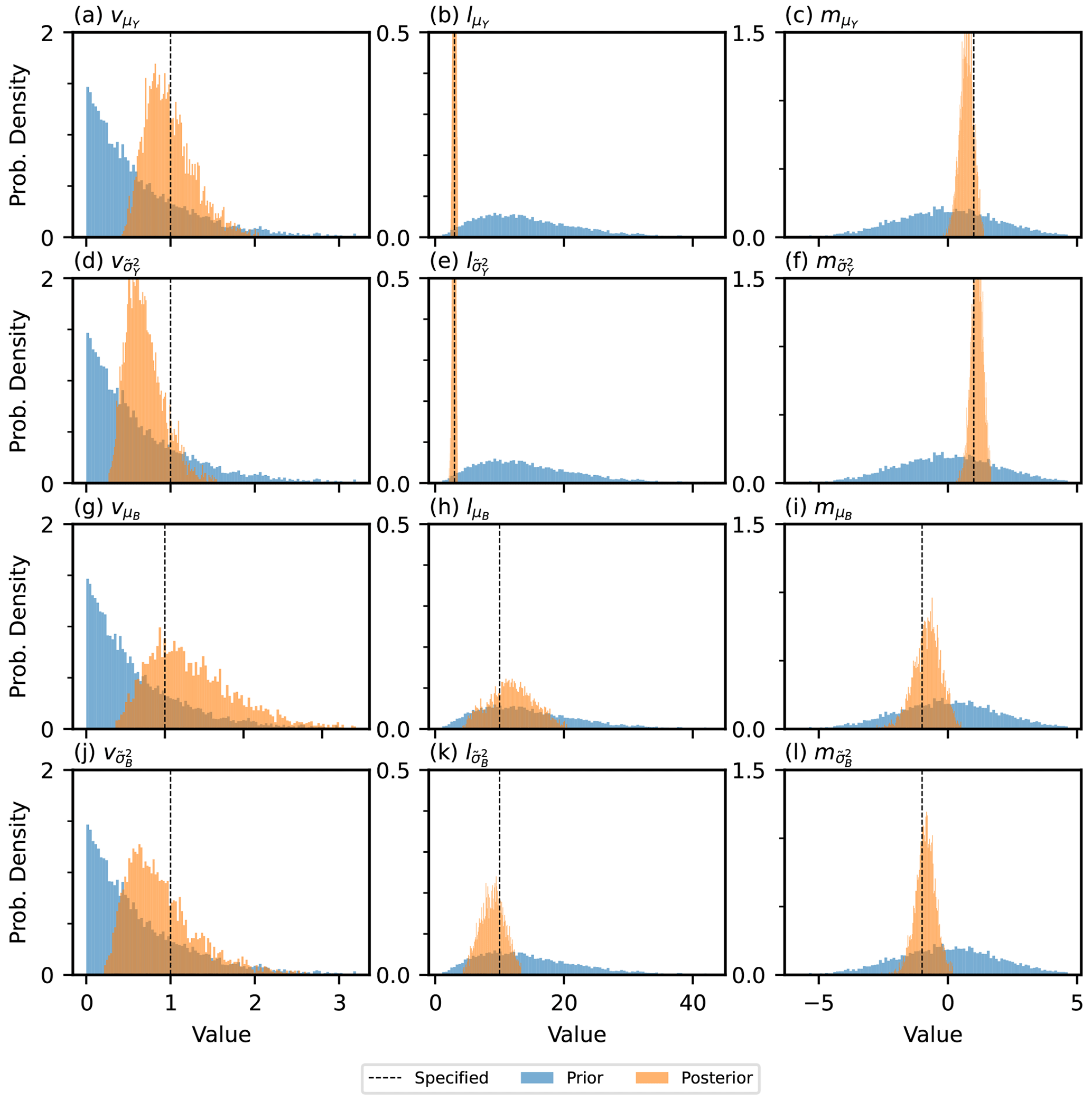
Figure F2A figure illustrating the prior and posterior distributions for the parameters of the model in the case of the one-dimensional hierarchical example. The value that was specified when generating the data is also shown.
Real-world scenarios are expected to have more complex spatial features than the simulated examples presented in Sect. 4.1, with the expectation that some of the assumptions of the model will partially broken, such as stationarity and independence of the latent processes. To explore the performance of the methodology under scenarios with more complex spatial features, as in real-world problems, results for several additional simulated examples (A–D) are presented in Fig. G1. The hyper-parameter values used to generate the data are presented in Table G1, while the summary statistics for the posterior distributions after fitting the model proposed in this paper are presented in Table G2.
Scenario A represents a potential real-world scenario where the covariance length scale changes across the domain. This could be due to topographic features and a shift from relatively smooth topography to sharp mountainous terrain. For this scenario, the length scale of the latent unbiased process changes abruptly at x=50, with a length scale of 5 for x<50 and a length scale of 1 for x>50. The length scale of the biased process remains constant across the domain in scenario A, although in scenario B it is made to also change abruptly at x=50 to simulate a case where the latent spatial structure of the bias is also dependent on an extra factor, such as topography.
Scenario C represents the potential real-world scenario where there are multiple sources of variation in the climate with different covariance length scales. An example of this could be the combined influence of large-scale upper-atmosphere circulation patterns and small-scale topographic changes over the domain. The data are generated from the unbiased process after defining the kernel as the sum of two independent components, one with a variance of 1 and length scale of 3 and the other with a variance of 0.2 and length scale of 0.6. Finally, scenario D represents a potential real-world case where the bias in the studied parameter is dependent on the parameter value itself, as might be the case if, for example, the output from temperature sensors were skewed by overheating. This correlation is induced between the bias and the unbiased process by generating the data for the bias as the sum , where is an independent bias, as generated in the other examples.
The result of fitting the model presented in this paper to each scenario is displayed in Table G2 and Fig. G1. From Table G2 it is clear that, in cases where multiple length scales are used in generating the data, the expected value of the assumed single length scale is in between the true values, tending more to the smallest length scale. The reason the expectation of the single length scale tends towards the shorter values present in generating the data is hypothesised to be the result of more spatial features (peaks and troughs) being present for the shorter length scale component. The model is able to explain the data observed better with a length scale closer to the shortest value present and the 95 % credible interval for the single length scale does not necessarily cover the multiple values used in generating the data.
In Fig. G1, it can be seen that, despite the additional complexities, the predictions of the unbiased parameter and of the bias are reasonable and capture the main spatial patterns. This demonstrates the flexibility of GPs and the robustness of the methodology proposed when attempting to fit different types of real-world data where some of the assumptions made in the model partially do not hold. Some features of the results are described here due to not fully capturing the dependencies involved in generating the data. In scenario A, the length scale of the unbiased process is estimated to be close to the value used in generating the data for x>50, which results in greater uncertainty than expected between nearby observations in the region of x<50, where the length scale is greater. For example, in the extrapolation range of x<0, the prediction in the unbiased parameter values returns sharply to the mean, with uncertainty independent of observed points, whereas if the length scale was correctly estimated in this region, the predictions would remain dependent on the data observed at x=0–10 for longer. The same is true in scenario B, with the addition of the estimates of the bias being effected, making disaggregating the climate model output into an unbiased and biased component more challenging, as seen at x=30. In scenario C, again, by only modelling a single length scale for the unbiased process, disaggregating the climate model output into its two components is effected and the longer length scale peak present at x=20 is attributed to the bias incorrectly. Finally, in scenario D, not accounting for the correlation between the unbiased values and the bias results in a slightly greater uncertainty in predictions than could be achieved by incorporating this relationship.
Overall, the model is shown to perform adequately and not be overly sensitive to some of the assumptions being partially broken, which supports the notion that the methodology is useful for real-world applications. In addition, other methodologies currently applied to bias correction are likely more affected in these complex scenarios. It is noted that the purpose of this paper is not to provide a final fixed model, however, instead aiming to provide a framework where additional complexities present in real-world applications can be assessed on a case-by-case basis and further model adjustments made where needed to account for specific features of the real-world data set. The model could be modified for each scenario to take into account the extra complexity, which is something that a fixed-type model for bias correction would not be able to handle.
Table G1A table showing the hyper-parameters of the latent Gaussian processes used to generate the complete underlying realisations of ϕY(s⋆), ϕB(s⋆) and hence ϕZ(s⋆), as well as observations of ϕY(sy) and ϕZ(sz), on which inference is done for the additional scenarios. The number of observations representing in situ data and climate model output is also given.
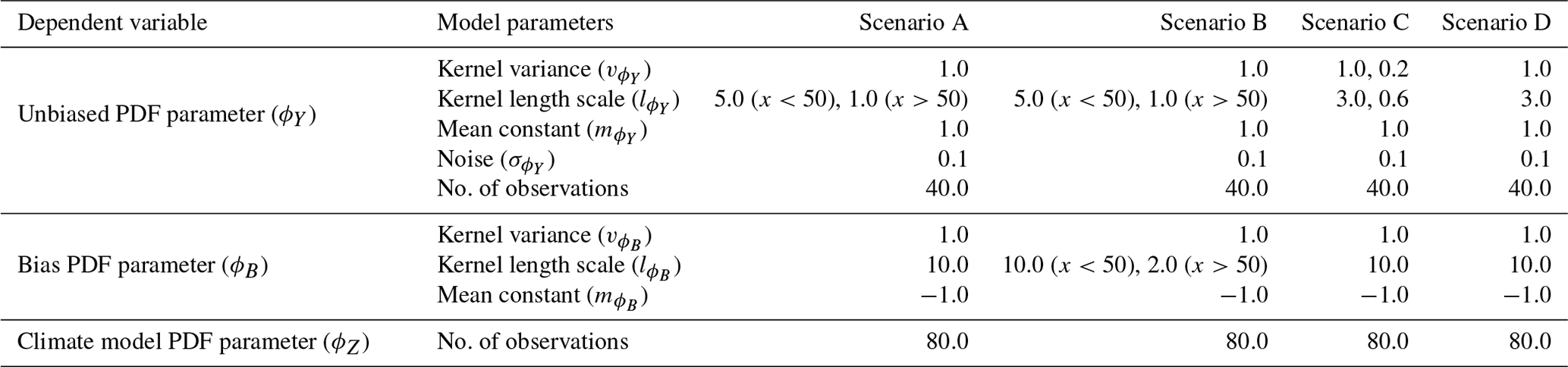
Table G2Tables showing summary statistics for the posterior distributions including the expectation (Exp.), standard deviation (SD), and lower and upper bounds for the 95 % credible interval (LCI and UCI). The prior distributions are the same non-informative distributions given in Table 3.
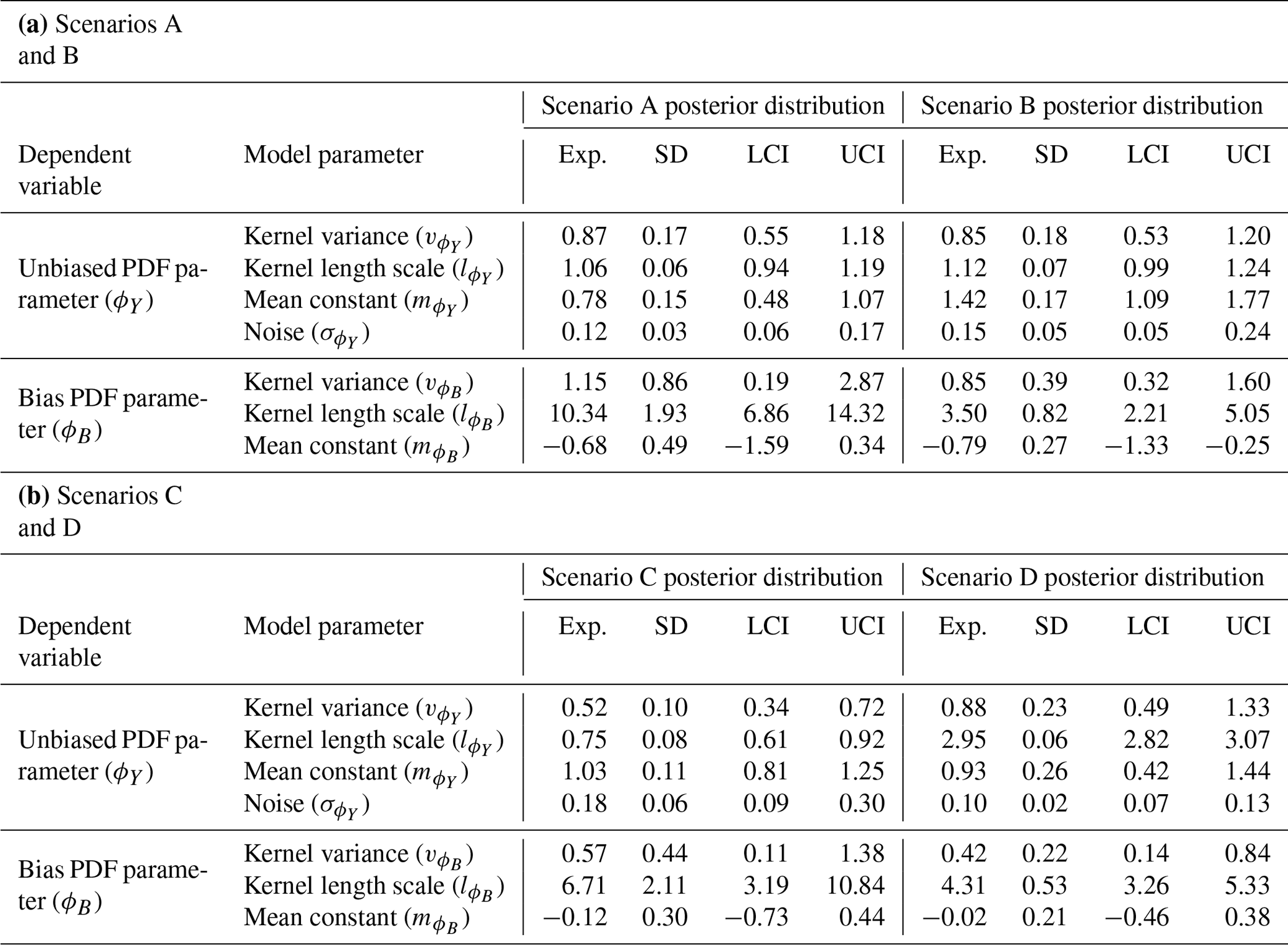
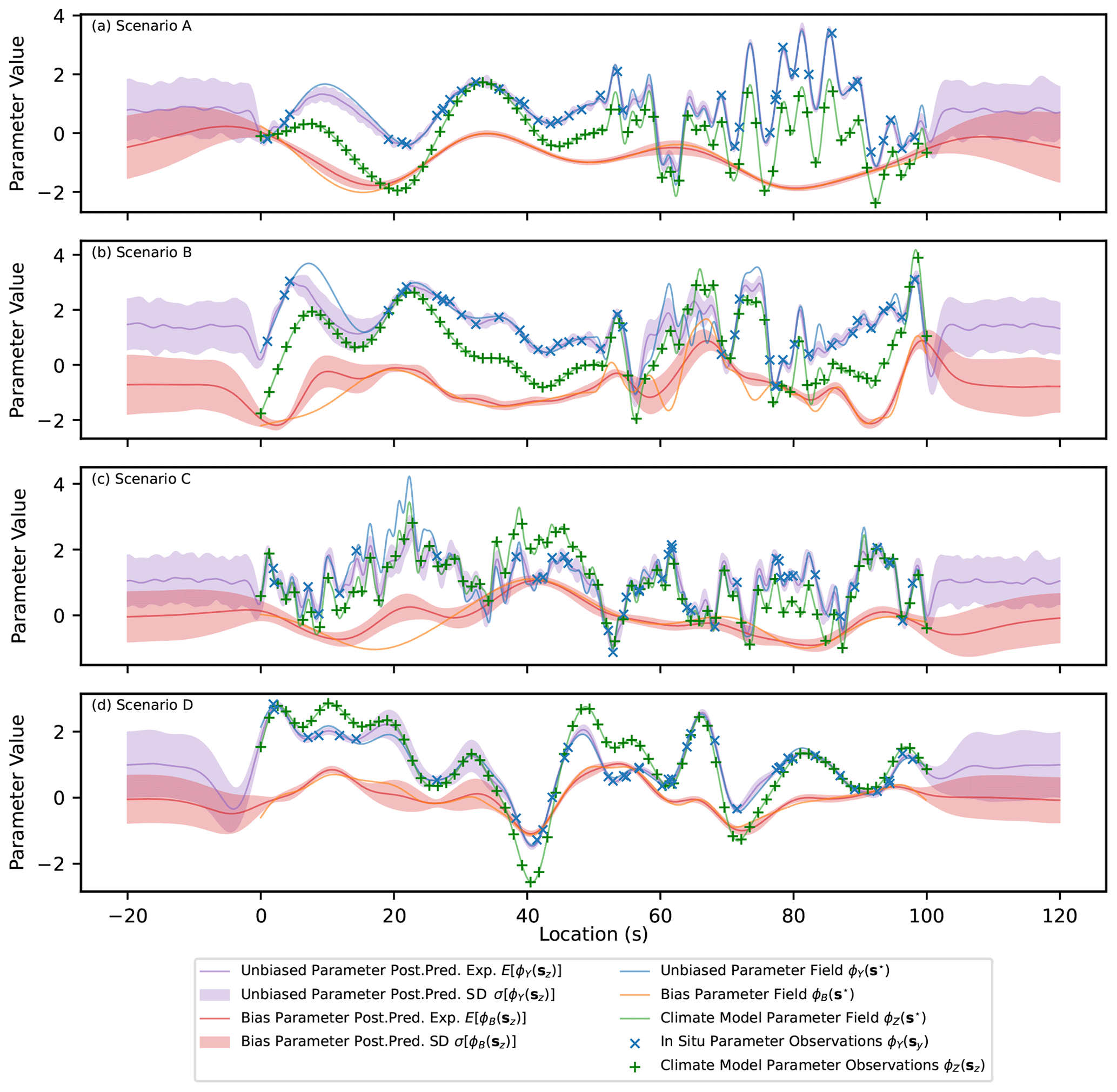
Figure G1Expectation and 1σ uncertainty in the posterior predictive distributions of the parameter ϕY(sz) and the corresponding bias, ϕB(sz), for three scenarios. The underlying functions (complete realisations) as well as the simulated input data are also shown.
The code used to generate the simulated data, fit the model, make predictions and create the figures/tables is available at https://doi.org/10.5281/zenodo.10053653 (Carter, 2023a). The data used to create the plots are available at https://doi.org/10.5281/zenodo.10053531 (Carter, 2023b).
JC: conceptualisation, methodology, software, validation, formal analysis and writing (original draft). ECM: conceptualisation, methodology, software, validation, formal analysis, writing (review and editing) and supervision. AL: conceptualisation, writing (review and editing) and supervision.
The contact author has declared that none of the authors has any competing interests.
Publisher’s note: Copernicus Publications remains neutral with regard to jurisdictional claims made in the text, published maps, institutional affiliations, or any other geographical representation in this paper. While Copernicus Publications makes every effort to include appropriate place names, the final responsibility lies with the authors.
Jeremy Carter and Amber Leeson are supported by the Data Science for the Natural Environment project (EPSRC; grant no. EP/R01860X/1). The code for analysis is written in Python 3.9.13 and makes extensive use the following libraries: NumPyro (Phan et al., 2019), TinyGP (Foreman-Mackey, 2023), NumPy (Harris et al., 2020) and Matplotlib (Hunter, 2007).
This research has been supported by the Engineering and Physical Sciences Research Council (grant no. EP/R01860X/1).
This paper was edited by Dan Lu and reviewed by Ziyi Yin and two anonymous referees.
Bader, D., Covey, C., Gutowski, W., Held, I., Kunkel, K., Miller, R., Tokmakian, R., and Zhang, M.: Climate Models: An Assessment of Strengths and Limitations, Climate Models: An Assessment of Strengths and Limitations, ISBN 9781507847190, 2008. a
Beyer, R., Krapp, M., and Manica, A.: An empirical evaluation of bias correction methods for palaeoclimate simulations, Clim. Past, 16, 1493–1508, https://doi.org/10.5194/cp-16-1493-2020, 2020. a, b
Carter, J.: Bias Correction of Climate Models using a Bayesian Hierarchical Model: Code, Zenodo [code], https://doi.org/10.5281/zenodo.10053653, 2023a. a
Carter, J.: Data used in generation of results in “Bias Correction of Climate Models using a Bayesian Hierarchical Model” J.Carter et. al., Zenodo [data set], https://doi.org/10.5281/zenodo.10053531, 2023b. a
Carter, J., Leeson, A., Orr, A., Kittel, C., and van Wessem, M.: Variability in Antarctic surface climatology across regional climate models and reanalysis datasets, The Cryosphere, 16, 3815–3841, https://doi.org/10.5194/tc-16-3815-2022, 2022. a, b
Cattiaux, J., Douville, H., and Peings, Y.: European temperatures in CMIP5: origins of present-day biases and future uncertainties, Clim. Dynam., 41, 2889–2907, https://doi.org/10.1007/s00382-013-1731-y, 2013. a
Das, A., Rokaya, P., and Lindenschmidt, K.-E.: The impact of a bias-correction approach (delta change) applied directly to hydrological model output when modelling the severity of ice jam flooding under future climate scenarios, Climatic Change, 172, 19, https://doi.org/10.1007/s10584-022-03364-5, 2022. a, b
Datta, A., Banerjee, S., Finley, A. O., and Gelfand, A. E.: Hierarchical Nearest-Neighbor Gaussian Process Models for Large Geostatistical Datasets, J. Am. Stat. Assoc., 111, 800–812, https://doi.org/10.1080/01621459.2015.1044091, 2016. a
DeConto, R. M. and Pollard, D.: Contribution of Antarctica to past and future sea-level rise, Nature, 531, 591–597, https://doi.org/10.1038/nature17145, 2016. a
Doblas-Reyes, F. J., Sörensson, A. A., Almazroui, M., Dosio, A., Gutowski, W. J., Haarsma, R., Hamdi, R., Hewitson, B., Kwon, W.-T., Lamptey, B. L., Maraun, D., Stephenson, T. S., Takayabu, I., Terray, L., Turner, A., and Zuo, Z.: Linking global to regional climate change, in: Climate Change 2021: The Physical Science Basis. Contribution of Working Group I to the Sixth Assessment Report of the Intergovernmental Panel on Climate Change, edited by: Masson-Delmotte, V., Zhai, P., Pirani, A., Connors, S. L., Péan, C., Berger, S., Caud, N., Chen, Y., Goldfarb, L., Gomis, M. I., Huang, M., Leitzell, K., Lonnoy, E., Matthews, J. B. R., Maycock, T. K., Waterfield, T., Yelekçi, O., Yu, R., and Zhou, B., Cambridge University Press, Cambridge, United Kingdom and New York, NY, USA, 1363–1512, https://doi.org/10.1017/9781009157896.001, 2021. a
Ehret, U., Zehe, E., Wulfmeyer, V., Warrach-Sagi, K., and Liebert, J.: HESS Opinions “Should we apply bias correction to global and regional climate model data?”, Hydrol. Earth Syst. Sci., 16, 3391–3404, https://doi.org/10.5194/hess-16-3391-2012, 2012. a, b, c, d, e
Flato, G., Marotzke, J., Abiodun, B., Braconnot, P., Chou, S. C., Collins, W., Cox, P., Driouech, F., Emori, S., Eyring, V., Forest, C., Gleckler, P., Guilyardi, E., Jakob, C., Kattsov, V., Reason, C., and Rummukainen, M.: Evaluation of Climate Models, in: Climate Change 2013 – The Physical Science Basis: Working Group I Contribution to the Fifth Assessment Report of the Intergovernmental Panel on Climate Change, edited by: Intergovernmental Panel on Climate Change (IPCC), Cambridge University Press, Cambridge, 741–866, ISBN 978-1-107-05799-9, https://doi.org/10.1017/CBO9781107415324.020, 2013. a, b
Foreman-Mackey, D.: dfm/tinygp: The tiniest of Gaussian Process libraries, Zenodo [code], https://doi.org/10.5281/zenodo.7646759, 2023 a
Giorgi, F.: Thirty Years of Regional Climate Modeling: Where Are We and Where Are We Going next?, J. Geophys. Res.-Atmos., 124, 5696–5723, https://doi.org/10.1029/2018JD030094, 2019. a, b
Greeves, C., Pope, V., Stratton, R., and Martin, G.: Representation of Northern Hemisphere winter storm tracks in climate models, Clim. Dynam., 28, 683–702, https://doi.org/10.1007/s00382-006-0205-x, 2007. a
Guilyardi, E., Wittenberg, A., Fedorov, A., Collins, C., Capotondi, A., Van Oldenborgh, G. J., and Stockdale, T.: Understanding El Niño in Ocean-Atmosphere General Circulation Models: Progress and Challenges, B. Am. Meteorol. Soc., 90, 325–340, https://doi.org/10.1175/2008BAMS2387.1, 2009. a
Haerter, J. O., Hagemann, S., Moseley, C., and Piani, C.: Climate model bias correction and the role of timescales, Hydrol. Earth Syst. Sci., 15, 1065–1079, https://doi.org/10.5194/hess-15-1065-2011, 2011. a
Harris, C. R., Millman, K. J., van der Walt, S. J., Gommers, R., Virtanen, P., Cournapeau, D., Wieser, E., Taylor, J., Berg, S., Smith, N. J., Kern, R., Picus, M., Hoyer, S., van Kerkwijk, M. H., Brett, M., Haldane, A., del Río, J. F., Wiebe, M., Peterson, P., Gérard-Marchant, P., Sheppard, K., Reddy, T., Weckesser, W., Abbasi, H., Gohlke, C., and Oliphant, T. E.: Array programming with NumPy, Nature, 585, 357–362, https://doi.org/10.1038/s41586-020-2649-2, 2020. a
Hensman, J., Matthews, A. G., Filippone, M., and Ghahramani, Z.: MCMC for Variationally Sparse Gaussian Processes, in: Advances in Neural Information Processing Systems, vol. 28, Curran Associates, Inc., https://proceedings.neurips.cc/paper_files/paper/2015/hash/6b180037abbebea991d8b1232f8a8ca9-Abstract.html (last access: 24 March 2024), 2015. a
Hoffman, M. D. and Gelman, A.: The No-U-Turn Sampler: Adaptively Setting Path Lengths in Hamiltonian Monte Carlo, J. Mach. Learn. Re., 15, 1593–1623, http://jmlr.org/papers/v15/hoffman14a.html (last access: 11 October 2023), 2014. a
Hourdin, F., Mauritsen, T., Gettelman, A., Golaz, J.-C., Balaji, V., Duan, Q., Folini, D., Ji, D., Klocke, D., Qian, Y., Rauser, F., Rio, C., Tomassini, L., Watanabe, M., and Williamson, D.: The Art and Science of Climate Model Tuning, B. Am. Meteorol. Soc., 98, 589–602, https://doi.org/10.1175/BAMS-D-15-00135.1, 2017. a
Hunter, J. D.: Matplotlib: A 2D Graphics Environment, Comput. Sci. Eng., 9, 90–95, https://doi.org/10.1109/MCSE.2007.55, 2007. a
Lima, C. H. R., Kwon, H.-H., and Kim, Y.-T.: A Bayesian Kriging model applied for spatial downscaling of daily rainfall from GCMs, J. Hydrol., 597, 126095, https://doi.org/10.1016/j.jhydrol.2021.126095, 2021. a, b, c, d, e, f, g, h, i, j
Liu, M., Rajagopalan, K., Chung, S. H., Jiang, X., Harrison, J., Nergui, T., Guenther, A., Miller, C., Reyes, J., Tague, C., Choate, J., Salathé, E. P., Stöckle, C. O., and Adam, J. C.: What is the importance of climate model bias when projecting the impacts of climate change on land surface processes?, Biogeosciences, 11, 2601–2622, https://doi.org/10.5194/bg-11-2601-2014, 2014. a, b
Maraun, D.: Bias Correcting Climate Change Simulations – a Critical Review, Current Climate Change Reports, 2, 211–220, https://doi.org/10.1007/s40641-016-0050-x, 2016. a, b
Mendez, M., Maathuis, B., Hein-Griggs, D., and Alvarado-Gamboa, L.-F.: Performance Evaluation of Bias Correction Methods for Climate Change Monthly Precipitation Projections over Costa Rica, Water, 12, 482, https://doi.org/10.3390/w12020482, 2020. a
Phan, D., Pradhan, N., and Jankowiak, M.: Composable Effects for Flexible and Accelerated Probabilistic Programming in NumPyro, arXiv [preprint], https://doi.org/10.48550/arXiv.1912.11554, 2019. a, b, c
Qian, W. and Chang, H. H.: Projecting Health Impacts of Future Temperature: A Comparison of Quantile-Mapping Bias-Correction Methods, Int. J. Environ. Res. Pub. He., 18, 1992, https://doi.org/10.3390/ijerph18041992, 2021. a, b, c
Rasmussen, C. E.: Gaussian Processes in Machine Learning, in: Advanced Lectures on Machine Learning: ML Summer Schools 2003, Canberra, Australia, February 2–14 2003, Tübingen, Germany, August 4–16 2003, Revised Lectures, edited by: Bousquet, O., von Luxburg, U., and Rätsch, G., Lecture Notes in Computer Science, Springer, Berlin, Heidelberg, 63–71, ISBN 978-3-540-28650-9, https://doi.org/10.1007/978-3-540-28650-9_4, 2004. a
Räty, O., Räisänen, J., and Ylhäisi, J. S.: Evaluation of delta change and bias correction methods for future daily precipitation: intermodel cross-validation using ENSEMBLES simulations, Clim. Dynam., 42, 2287–2303, https://doi.org/10.1007/s00382-014-2130-8, 2014. a
Sippel, S., Otto, F. E. L., Forkel, M., Allen, M. R., Guillod, B. P., Heimann, M., Reichstein, M., Seneviratne, S. I., Thonicke, K., and Mahecha, M. D.: A novel bias correction methodology for climate impact simulations, Earth Syst. Dynam., 7, 71–88, https://doi.org/10.5194/esd-7-71-2016, 2016. a
Tebaldi, C., Debeire, K., Eyring, V., Fischer, E., Fyfe, J., Friedlingstein, P., Knutti, R., Lowe, J., O'Neill, B., Sanderson, B., van Vuuren, D., Riahi, K., Meinshausen, M., Nicholls, Z., Tokarska, K. B., Hurtt, G., Kriegler, E., Lamarque, J.-F., Meehl, G., Moss, R., Bauer, S. E., Boucher, O., Brovkin, V., Byun, Y.-H., Dix, M., Gualdi, S., Guo, H., John, J. G., Kharin, S., Kim, Y., Koshiro, T., Ma, L., Olivié, D., Panickal, S., Qiao, F., Rong, X., Rosenbloom, N., Schupfner, M., Séférian, R., Sellar, A., Semmler, T., Shi, X., Song, Z., Steger, C., Stouffer, R., Swart, N., Tachiiri, K., Tang, Q., Tatebe, H., Voldoire, A., Volodin, E., Wyser, K., Xin, X., Yang, S., Yu, Y., and Ziehn, T.: Climate model projections from the Scenario Model Intercomparison Project (ScenarioMIP) of CMIP6, Earth Syst. Dynam., 12, 253–293, https://doi.org/10.5194/esd-12-253-2021, 2021. a
Teutschbein, C. and Seibert, J.: Bias correction of regional climate model simulations for hydrological climate-change impact studies: Review and evaluation of different methods, J. Hydrol., 456-457, 12–29, https://doi.org/10.1016/j.jhydrol.2012.05.052, 2012. a
Wang, Y. and Chaib-draa, B.: An online Bayesian filtering framework for Gaussian process regression: Application to global surface temperature analysis, Expert Syst. Appl., 67, 285–295, https://doi.org/10.1016/j.eswa.2016.09.018, 2017. a
Zhang, Y., Feng, M., Zhang, W., Wang, H., and Wang, P.: A Gaussian process regression-based sea surface temperature interpolation algorithm, J. Ocean. Limnol., 39, 1211–1221, https://doi.org/10.1007/s00343-020-0062-1, 2021. a
- Abstract
- Introduction
- Methodology
- Data generation
- Results
- Discussion
- Conclusion
- Appendix A: Bias in climate models
- Appendix B: Capturing spatial structure with Gaussian processes
- Appendix C: Posterior and posterior predictive formulation
- Appendix D: Specific example with temperature
- Appendix E: Shared- and single-process model comparison
- Appendix F: Prior and posterior hyper-parameter distributions
- Appendix G: Complex scenarios
- Code and data availability
- Author contributions
- Competing interests
- Disclaimer
- Acknowledgements
- Financial support
- Review statement
- References