the Creative Commons Attribution 4.0 License.
the Creative Commons Attribution 4.0 License.
 | 19 Jun 2024
Assessing effects of climate and technology uncertainties in large natural resource allocation problems
Jevgenijs Steinbuks
Yongyang Cai
Jonas Jaegermeyr
Thomas W. Hertel
The productivity of the world's natural resources is critically dependent on a variety of highly uncertain factors, which obscure individual investors and governments that seek to make long-term, sometimes irreversible, investments in their exploration and utilization. These dynamic considerations are poorly represented in disaggregated resource models, as incorporating uncertainty into large-dimensional problems presents a challenging computational task. In this paper, we apply the SCEQ algorithm (Cai and Judd, 2023) to solve a large-scale dynamic stochastic global land resource use problem with stochastic crop yields due to adverse climate impacts and limits on further technological progress. For the same model parameters and bounded shocks, the range of land conversion is considerably smaller for the dynamic stochastic model than for deterministic scenario analysis.
- Article
(2847 KB) - Full-text XML
- BibTeX
- EndNote


Understanding the future allocation of the world's natural resources is an important research problem for environmental scientists and economists. This involves a thorough understanding of a complex interplay of different factors, including, among others, continuing population increases, shifting diets among the poorest populations in the world, increasing production of renewable energy, including biofuels, and growing demand for ecosystem services, including forest carbon sequestration (Foley et al., 2011). The problem is further confounded by faster-than-expected climate change which is altering the biophysical environment of agriculture and forestry. Moreover, highly uncertain future productivities and valuations of ecosystem services, coupled with medium- to long-term irreversibilities in the extraction of nonrenewable or partially renewable resources, such as long-growth natural forests, give rise to a challenging problem of decision-making under uncertainty.
While there is a large body of research analyzing the problem of natural resource extraction and utilization under uncertainty theoretically or using stylized computational models (see, e.g., Miranda and Fackler, 2004; Tsur and Zemel, 2014, and references therein), quantifying the effects of uncertainty in the natural resource use in a more realistic setting remains a challenging problem. This is because natural resource allocation problems, like environmental policy problems in general, involve highly nonlinear structure and damage functions, important irreversibilities, and long time horizons (Pindyck, 2007). Computationally integrated models of economy and environment are the standard workhorse mechanisms for modeling the long-term allocation of the world's natural resources, including particularly difficult land use problems (see, e.g., Füssel, 2009; Schmitz et al., 2014; Nikas et al., 2019, and references therein). These models have the important advantage of detailed spatial and sectoral (particularly in the energy and agricultural sector) coverage, which allows them to capture a broad range of responses to changes in demand and supply factors affecting the utilization of natural resources. However, given the high computational complexity of these models, they are typically either static or based on myopic expectations, whereby decisions about production, consumption, and resource extraction and conversion are made only on the basis of information in the period of the decision (Babiker et al., 2009). These models, therefore, have limited ability to address important intertemporal questions such as, for example, a dynamic trade-off between conservation, carbon sequestration, and renewable offsets for fossil fuels. Among the few forward-looking dynamic economy and environment models, none explicitly incorporates uncertainty into the determination of the optimal path of natural resource use.1 This is because introducing uncertainty into these models is confined by an array of computational obstacles that are very difficult (e.g., high dimensionality and kinks caused by occasionally binding constraints), if not impossible, to address using standard numerical methods such as projection methods and value function iteration (see, e.g., Judd, 1998; Miranda and Fackler, 2004; Cai and Judd, 2014; Cai, 2019). To the extent that uncertainty in these models is considered, this is only through parametric or probabilistic sensitivity analysis or the use of alternative scenarios. Therefore, the high-dimensional resource use models have not effectively dealt with optimal extraction and conversion decisions along the uncertain path of key drivers affecting resource allocation in the face of costly reversal of conversion decisions.
In this study, we seek to address this important limitation of the economy–environment modeling of natural resource use. In doing so, we build on recent advances in computational economic and operation research. Cai et al. (2017) introduced a nonlinear certainty equivalent approximation method (NLCEQ) for solving large-scale, infinite-horizon stationary dynamic stochastic problems and demonstrated how this method could be used to achieve an accurate solution to a stylized stationary dynamic stochastic land use problem. The original NLCEQ method, however, is ill-suited for solving most environmental and resource economic problems. This is because stochastic problems of the utilization of natural resources feature nonstationary stochastic trends, such as climate or technological trajectories, and some never converge to a stationary state. Building on the original NLCEQ work Cai and Judd (2023) introduced a simulated certainty equivalent approximation method (SCEQ), which efficiently solves nonstationary dynamic stochastic problems, including those with high dimensionality and occasionally binding constraints. Cai and Judd (2023) showed that the SCEQ method is highly accurate and achieves stable numerical solutions for dynamic stochastic problems in economics.
We apply the SCEQ method to solve a large-scale dynamic stochastic model, focusing on the optimal global land use allocation problem. This highly complicated resource use problem features multiple cross-sectoral and dynamic trade-offs. Specifically, we apply the method to a global land use model nicknamed FABLE (Forest, Agriculture, and Biofuels in a Land use model with Environmental services) in the face of uncertainty. FABLE is a dynamic, forward-looking, global, multi-sectoral, and partial-equilibrium model designed to analyze the evolution of global land use over the coming century. Prior applications of that model (Steinbuks and Hertel, 2013; Hertel et al., 2013, 2016; Steinbuks and Hertel, 2016) analyze the competition for scarce global land resources in light of the growing demand for food, energy, forestry, and environmental services and evaluate key drivers and policies affecting global land use allocation. All of these applications, however, assume perfect foresight and treat uncertainty in a parametric fashion, thus ignoring the impact of future uncertainties in the optimal allocation of global land use. To ensure consistency between theoretical and numerical model solutions, we assume the bounded solution space. As we show below, this assumption is well justified for economic models of large natural resource allocation problems, including the FABLE model.
By way of illustration, we focus on uncertainty emanating from crop productivity over the next century. Along with energy prices, regulatory policies, and technological change in food, timber, and biofuels industries, this is one of four core uncertainties affecting competition for global land use (Steinbuks and Hertel, 2013). To quantify the uncertainty in agricultural yields, we construct a stochastic crop productivity index that captures two key uncertainty sources: technological progress and global climate change (Lobell et al., 2009; Licker et al., 2010; Foley et al., 2011).2 Following Rosenzweig et al. (2014), we use projections from climate and crop-simulation models under Representative Concentration Pathways 6.0 W m−2 (RCP6) greenhouse gas (GHG)-forcing scenario (Moss et al., 2008), as well as the survey of recent agro-economic and biophysical studies to calibrate the index.
We simulate the results of the model, where the global planner optimally allocates land uses under the perfect foresight of different realizations of the crop productivity index, focusing our attention on the current century. We then compare and contrast them with the results of the dynamic stochastic model, where the global planner has rational expectations about crop yields subject to bounded autocorrelated climate shocks. When the uncertainty in crop productivity is incorporated into the model, we see an additional redistribution of land resources to offset the impact of potentially lower yields. Due to intertemporal substitution, some of that redistribution occurs even in the absence of actual changes in the states of climate or technology affecting crop yields. Moreover, the range of these alternative optimal paths of cropland is considerably smaller than the magnitude of possible land conversion resulting from the scenario analysis based on the deterministic model. This result indicates that when the climate shocks are bounded, the scenario analysis may significantly overstate the expected agricultural land conversion magnitude under uncertain crop yields.
Our study contributes to the growing literature that analyzes the intertemporal allocation of land and other natural resources under uncertainty and irreversibility constraints. Most of the literature focuses on a particular type of resource or sector in which intertemporal issues are significant and cannot be ignored. One example of this literature is forestry management in the context of uncertain fire risks and climate mitigation policies (Sohngen and Mendelsohn, 2003, 2007; Daigneault et al., 2010). Another example is natural land conservation decisions under irreversible biodiversity losses (Conrad, 1997, 2000; Bulte et al., 2002; Leroux et al., 2009). While these models are undoubtedly helpful for understanding the broad implications of uncertainty in the intertemporal allocation of land resources, they are less effective in quantifying the effect of uncertainty in the supply and demand drivers in more complex settings, such as, e.g., the optimal allocation of multiple competing land resources in the long run.
Our study is perhaps most closely related to the recent works of Lanz et al. (2017) and Zhao et al. (2021). Lanz et al. (2017) developed a two-sector stochastic Schumpeterian growth model with the endogenous allocation of global land use. As our paper does, they find that the optimal allocation of global land use requires more cropland conversion when the uncertainty in agricultural productivity is present. Lanz et al. (2017), however, focused on endogenous population dynamics, labor allocation, and technological progress, whereas our paper is concerned with the endogenous allocation of multiple types of land use and corresponding land-based goods and services. Our paper also advances the methodological grounds by applying a more advanced algorithm that overcomes computational difficulties in solving multidimensional stochastic land use models, which made Lanz et al. (2017) significantly simplify their model by assuming that their binary shocks occur only in three time periods. Zhao et al. (2021) compare models with adaptative expectations and perfect foresight assumptions for both the price and yield for agricultural producers to make land allocation and production decisions. Zhao et al. (2021) find similar results that land use change variation becomes much smaller than in the perfect foresight model, which allows for faster land use adjustments while market price variations increase. Unlike our paper, Zhao et al. (2021) do not explicitly incorporate uncertainty in the model's optimization stage.
This section presents a modeling framework for analyzing nonlinear dynamic stochastic models of natural resource use with multiple sectors, in which preferences, production technology, resource endowments, and other exogenous state variables evolve stochastically over time according to a Markov process with time-varying transition probabilities. The constructed model belongs to the class of stochastic growth models, with multiple sectors studied in Brock and Majumdar (1978), Majumdar and Radner (1983), and Stokey et al. (1989) among others. Similar to other models in this class, the FABLE model has a bounded solution space, as all these models are theoretically shown to have equilibrium paths (Stokey et al., 1989). This assumption is important because it is often impossible to prove that in the presence of unbounded solution space, the stochastic model has a finite solution. For example, Weitzman's dismal theorem (Weitzman, 2010) shows that a fat-tail damage function with an infinite upper bound leads to an infinite risk premium, but a numerical truncation to finite support will always have a finite risk premium. So, assuming the bounded solution space is necessary for avoiding the potential qualitative inconsistencies between their theoretical and numerical results. We further discuss the assumption of the bounded solution space in the FABLE model in Sect. 5.
Specifically, we develop a stochastic version of a global land use model nicknamed FABLE (Forest, Agriculture, and Biofuels in a Land use model with Environmental services), a dynamic multi-sectoral model for the world's land resources over the next century (Steinbuks and Hertel, 2012, 2016). This model combines recent strands of agronomic, economic, and biophysical literature into a single intertemporally consistent analytical framework at the global scale. FABLE is a discrete dynamic partial-equilibrium model where the population, labor, physical and human capital, and other variable inputs are assumed to be exogenous. Total factor productivity and technological progress in non-land-intensive sectors are also predetermined. The model focuses on the optimal allocation of scarce land across competing uses across time and solves the dynamic paths of alternative land uses, which together maximize global economic welfare.
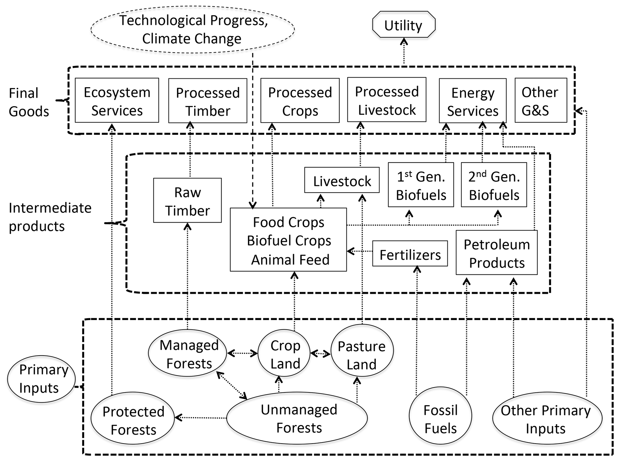
Figure 1Structure of the FABLE Model. Note that state variables are shown as oval shapes. Decision variables are shown as rectangular shapes. The utility function is shown as an octagonal shape. Stochastic model terms incorporating random processes are shown as dashed shapes or arrows.
The FABLE model accommodates a complex dynamic interplay between different types of global land use, whereby the societal objective function places value on processed crops and livestock, energy services, timber products, ecosystem services, and other non-land goods and services (Fig. 1). There are three accessible primary resources in this partial-equilibrium model of the global economy: land, liquid fossil fuels, and other primary inputs, e.g., labor and capital (see the bottom part of Fig. 1). The supply of land is fixed and faces competing uses that are determined endogenously by the model. They include unmanaged forest lands which are in an undisturbed state (e.g., parts of the Amazon tropical rainforest ecosystem), agricultural (or crop) land, pasture land, and commercially managed forest land. As trees of different ages have different timber yields and different propensities to sequester carbon, the model keeps track of various tree vintages in managed forests, which introduces additional numerical complexity for solving the model. We do not keep track of vintages for natural lands and assume they are primarily old-grown forests. We ignore other land use types, such as savannah, grasslands, and shrublands, which are largely unmanaged and often of limited productivity.3 We also ignore residential, retail, and industrial uses of land in this partial-equilibrium model of agriculture and forestry.
The flow of liquid fossil fuels evolves endogenously along an optimal extraction path, allowing exogenously specified new discoveries of fossil fuel reserves. Other primary inputs include variable inputs, such as labor, capital (both physical and human), and intermediate materials. The endowment of other primary inputs is exogenous and evolves along a pre-specified global economic growth path.
There are six intermediate inputs used in the production of land-based goods and services in FABLE: petroleum products, fertilizers, crops, liquid biofuels,4 live animals, and raw timber (see the middle part of Fig. 1). Fossil fuels are refined and converted to either petroleum products that are further combusted or to fertilizers that are used to boost yields in the agricultural sector. Cropland and fertilizers are combined to grow crops that can be further converted into processed food and biofuels or used as animal feed. Specifically, we assume that agricultural land and fertilizers are imperfect substitutes in the production of food crops, , with specific production technology given by the following constant elasticity of substitution (CES) function:
where is stochastic crop technology index, and αn and ρn are, respectively, the input share and substitution parameters. Equation (1) captures three key responses within the model to changes in crop technology index: (i) demand response (change in consumption of food crops), (ii) adaptation on the extensive margin (substitution of agricultural land for other land resources), and (iii) adaptation on the intensive margin (substitution of agricultural land for fertilizers).
Biofuels substitute imperfectly for liquid fossil fuels in final energy demand. The food crops used as animal feed and pasture land are combined to produce raw livestock. Harvesting managed forests yields raw timber that is further used in timber processing.
The land-based consumption goods and services take the form of processed crops, livestock, and timber and are, respectively, outcomes of food crops, raw livestock, and timber processing. The production of energy services combines non-land energy inputs (i.e., liquid fossil fuels) with biofuels, and the resulting mix is further combusted. Finally, all land types can contribute to other ecosystem services and a public good to society, including recreation, biodiversity, and other environmental goods and services. To close the demand system, we also include other non-land goods and services (e.g., manufacturing goods and retail, construction, financial, and information services), which involve the “consumption” of other primary inputs not spent on the production of land-based goods and services. As the model focuses on the representative agent's behavior, the final consumption products are all expressed in per capita terms.
A complete description of model equations, variables, and parameter values is presented in the Appendix.
This section characterizes uncertainty in future agricultural yields over the coming century, which is one of the core uncertainties shown to affect land use in the long run (Steinbuks and Hertel, 2013). Crop yields are subject to two types of uncertainties: those related to the development and dissemination of new technologies and those related to changes in the climatic conditions under which the crops are grown. The former type of uncertainty has until recently dominated the pattern of the evolution of global crop yields, whereas the latter is becoming an increasingly important factor (Lobell and Field, 2007; IPCC, 2014). While it is plausible to hypothesize that accelerating climate impacts may, in turn, induce further technological advances in an effort to facilitate adaptation to climate change, this hypothesis is not supported by limited empirical evidence (Burke and Emerick, 2016). Therefore, in this paper, these two sources of uncertainty are treated separately, although they are both characterized by the use of combined climate and crop-simulation models run over a global grid.
We characterize future uncertainty in yields by constructing a stochastic crop productivity index, , which captures the evolution of future crop yields under different realizations of uncertainty in crop productivity based on the most recent projections in the agronomic and environmental science studies. An important characteristic of staple grain yields is that they tend to grow linearly, adding a constant amount of gain (e.g., t ha−1) each year (Grassini et al., 2013). This suggests that the proportional growth rate should fall gradually over time. However, crop physiology dictates certain biophysical limits to the rate at which sunlight and soil nutrients can be converted to grain. And there is some recent agronomic evidence (Cassman et al., 2010; Grassini et al., 2013) showing that yields appear to be reaching a plateau in some of the world's most important cereal-producing countries. Cassman (1999) suggests that average national yields can be expected to plateau when they reach 70 %–80 % of the genetic yield potential ceiling. Based on these observations from the agronomic literature, we specify the following logistic function determining the evolution of the crop productivity index over time:
where is the value of the crop productivity index in period 0, which we calibrate to match observed weighted yields in key staple crops (corn, rice, soybeans, and wheat). is the crop yield potential at the end of the current century; that is, “the yield an adapted crop cultivar can achieve when crop management alleviates all abiotic and biotic stresses through optimal crop and soil management” (Evans and Fischer, 1999). κc is the logistic convergence rate to achieving potential crop yields.
Though the initial value of the crop productivity index is known with certainty, potential crop yields are highly uncertain. We assume that potential crop yields are affected by a two-dimensional stochastic process of climate and technological shocks, J1,t, and J2,t, respectively. For the technological shock, J2,t, we assume that there are three states of technology: “bad” (indexed by ), “medium” (indexed by ), and “good” (indexed by ). In the optimistic (i.e., good) state of advances in crop technology, we assume that yields will continue to grow linearly throughout the coming century, eliminating the yield gap by 2100. In the medium state of technology, rather than closing the yield gap by 2100, average yields in 2100 are just three-quarters of the yield potential at that point in time. In the bad state of technology, there is no technological progress, and the crop yields stay the same as at the beginning of the coming century.
For the climate shock, J1,t, we assume it is a Markov chain with five possible states at each time t. To construct these states, we use the results of Inter-Sectoral Impact Model Intercomparison Project (ISIMIP) fast-track crop-simulation model comparison (Rosenzweig et al., 2014).5 Since FABLE is a partial-equilibrium model without an embedded climate module, we cannot directly capture all sources of GHG emissions and endogenize their effect on global crop yields. Instead, to ensure the simulation results' comparability with the structural parameters (e.g., demographic and economic growth and the rate of technological change) of the FABLE model, we select four crop-simulation model runs under the RCP6 GHG forcing scenario.6 We also consider alternative assumptions on CO2 fertilization effects.
Based on these data, we construct five states corresponding to quintiles of the distribution of different outcomes of four global crop-simulation models and five global climate models, with and without CO2 fertilization effects for potential crop yields by 2100. Under two optimistic states of the world, we observe 2 % and 15 % increases in potential crop yields relative to the model baseline (calibrated based on historical trends over the reference period 1971 to 2004), respectively, whereby significant CO2 fertilization effects offset the negative effects of climate change. For the next two states, we see declines of 15 % and 19 % in potential crop yields relative to the model baseline, whereby CO2 fertilization effects are assumed to be either small or non-existent, and the negative effects of climate change tend to prevail. Finally, under the most pessimistic state of the world, drastic adverse effects of climate change combined with the absence of any CO2 fertilization effects result in a 36 % decline in potential crop yields relative to the model baseline.
Further details of constructing climate and technological states can be found in the Appendix.
The path of technological change in crop yields evolves by reversible transitions across these states. The stochastic path of the crop productivity index is then given by
where AT(i,j) represents the crop productivity index at the terminal time T at the state and for and . Thus, At is a Markov chain, which takes 1 of 15 possible time-varying values at each time period. This can be seen as a discretization of a mean-reverting process with continuous values and a time trend, but a finer Markov chain with more values can only marginally change our solution. As At is completely dependent on J1,t and J2,t, it is not a state variable, whereas J1,t and J2,t are both state variables.
Having characterized the realizations of crop productivity under alternative states of agricultural technology and climate change impacts, we still need to calibrate the transition probabilities for the climate and technology shocks to construct the stochastic crop productivity index. As regards climate shock, the environmental and climate science literature acknowledges some degree of persistence but does not provide much guidance on the transition dynamics between alternative climate states affecting crop yields. In the absence of reliable estimates for constructing the transition probability matrix of J1,t, we assume simple transition dynamics, where each state has a 50 % probability of retaining itself next period and a 25 % probability of moving upwards and downwards to an adjacent state (note that realizations can only stay the same or move upwards from the lowest state, e.g., , and only stay the same or move downwards from the highest state, e.g., ). As regards the technology shock, since we do not have historical data on the evolution of agricultural technology, we assume that technological advances in agriculture follow a similar trend to advances in the rest of the economy and use the probability transition matrix of J2,t estimated by Tsionas and Kumbhakar (2004) for a comprehensive panel of 59 countries over the period of 1965–1990. These estimates correspond to a 20 % probability of the bad technological state, 56 % of the medium state, and 24 % of the good state. The transition probability matrices of J1,t and J2,t are shown in the Appendix.
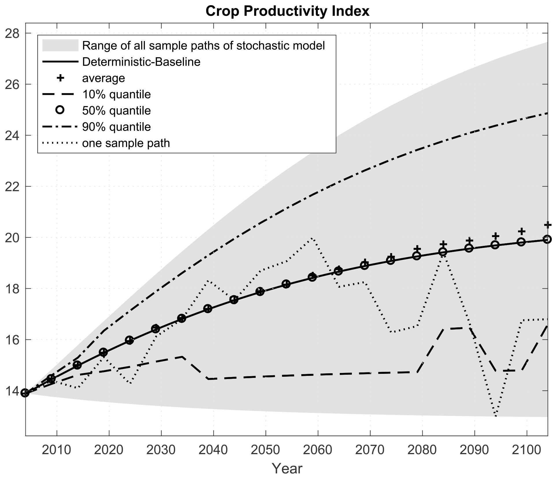
Figure 2 shows the deterministic-baseline path (the solid line) used in the perfect foresight model and the range of the stochastic crop productivity index based on 1000 simulation paths over the entire 21st century, with additional summary statistics presented in the Appendix. The simulations start at the medium states of climate and technology in the initial year. The deterministic-baseline path is calculated by taking expectations of the stochastic crop productivity index conditional on the initial medium states (Eq. 3). It also takes the same values as the median path (the “o” line) of simulations, whereby the climate and technological states are kept at medium, while the average line (the “+” line) deviates a bit after the year 2070. At every time t, there are 1000 realized values of At, among which there are only 15 different values. The 10 % and 90 % quantile lines (the dashed and dash-dotted lines) represent the 10 % and 90 % quantiles of these 1000 simulated values of At at time t, so they are not the realized sample paths, but Fig. 2 also displays one realized sample path of At, which is the dotted line.
In most resource use problems under uncertainty, including the FABLE model, the social planner's problem cannot be solved analytically, although certain inferences about the potential effects of uncertainty can be made from more stylized models. Numerical dynamic programming with value function iteration (see, e.g., Cai and Judd, 2014; Cai, 2019) is a typical method to solve these dynamic stochastic problems. However, numerical dynamic programming faces challenging problems such as high dimensionality of state space, shape-preservation of value functions (Cai and Judd, 2013), and kinks caused by occasionally binding constraints. These challenges are common in modeling natural resource use and are hard to address, even with the most advanced methods such as parallel dynamic programming (Cai et al., 2015).
For non-stationary problems, value function iteration involves computing decision rules at each period t. However, computing all these rules can be very time-consuming and unnecessary if our primary goal is to obtain simulation paths and their distributions until a time of interest, T*, even if it is a long one (in environmental and climate change economics, for example, we are often interested in solutions for the coming century and set the time of interest to 100 years and the problem horizon of more than 300 years to avoid a large impact of terminal conditions). Instead of solving for optimal decisions for all possible states at each time, we can approximately solve for optimal decisions for those simulated states along simulated paths. This logic is embedded in the novel SCEQ algorithm (Cai and Judd, 2023) used to solve for a simulated range of land use trajectories in the stochastic FABLE model.
Below we present the SCEQ algorithm version for solving the finite horizon nonstationary stochastic dynamic programming problems that the FABLE model belongs to (for a detailed description of other cases, see Cai and Judd, 2023). Following the standard notation in the literature, let St be a vector of state variables (here land cover types and stocks of fossil fuels), and let at be a vector of decision variables (here land conversion, resource extraction, transformation, and final consumption of land-based goods and services) at each time t. The transition law of the state vector S is
where ϵt is a serially uncorrelated random vector process, and Gt is a vector of functions; its ith element, Gt,i, returns the ith state variable at t+1: . For simplicity, we assume the mean of ϵt is 0.7
The FABLE model equations (see Appendix) can be compactly represented by the following social planner's problem:
where 𝒰t is a utility function, is the discount factor, 𝔼 is the expectation operator, T is the horizon (T=∞ if it is an infinite-horizon problem), VT(ST) is a given terminal value function depending on the terminal state ST (it is zero everywhere for an infinite-horizon problem), and is a vector of feasibility constraints of actions at at time t. And we assume that the initial state S0 is given, as it can usually be observed or estimated.
Algorithm 1SCEQ for finite-horizon stochastic dynamic programming problems with time-variant exogenous paths.
- Step 1.
-
Initialization step. Given the initial state S0 and a time of interest T*, as well as a terminal value function VT(ST), simulate a sequence of ϵt to get m paths, denoted for path i, from t=0 to . Let and iterate forward through steps 2 and 3 for .
- Step 2.
-
Optimization step. Solve the following deterministic model starting from time s and simulated node :
where Ss is given by , for each .
- Step 3.
-
Simulation step. Set , where is the optimal decision at time s of problem (5) for each .
Algorithm 1 obtains simulated pathways of optimal decisions and states. Note that the inside loop across i can be switched with the outside loop across time; that is, for each i, we can obtain one simulation path by iteratively solving Eq. (5) and simulating for .
The optimization step of Algorithm 1 applies the certainty equivalent approximation idea of the NLCEQ method (Cai et al., 2017); for a given state at time s, , we replace all future stochastic variables by their corresponding expectations conditional on the current state ,8 and convert the dynamic stochastic problem (4) into a deterministic finite-horizon dynamic problem (5).
We implement the optimal control method (Cai, 2019) to solve Eq. (5) numerically; that is, we view Eq. (5) as a large-scale nonlinear constrained optimization problem with and as its variables and the transition equations and feasibility restrictions as its constraints. The problem can be directly solved with an appropriate nonlinear optimization solver such as CONOPT (Drud, 1994).
Observe that we just need to save the solution of Eq. (5) at time s, , for use in the next step. In step 3 of Algorithm 1, we use the saved optimal decision to generate the next-period state, , given the realization of shocks, . Once we reach the state at time s+1, we come back to implement step 2 and then step 3. In other words, Algorithm 1 uses an adaptive management way; decisions are made for the current period in the face of future uncertain shocks. Once the next-period shock is observed, decisions for the next period are made with re-optimization, given the observed shock and new state variables at the next period. Observe that the serial correlation of random variables has been captured in their associated transition laws. Repeating this process iteratively through T* times, we compute a representative simulated pathway of optimal decisions, , and states, , which corresponds to the realized path of shocks, . Repeating over i, we compute m simulated paths of optimal states and decisions and then obtain their distributions. This simulation process can be naturally parallelized.
After we obtain the simulated solutions for our dynamic stochastic land use problem, we also check the normalized Euler errors and find that the ℒ1 error in the solutions for the first 100 years (the periods of interest) among 1000 simulated paths is only , and the corresponding ℒ∞ error is only 0.02. This is within range of acceptable accuracy for the most dynamic stochastic problems (Cai and Judd, 2023).
Below, we describe the results of the impact of crop yield uncertainty in the optimal path of global land use based on the dynamic stochastic model simulations. We solve the model over 400 years with 5-year time steps and present the results for the first 100 years to minimize the effect of terminal period conditions on our analysis.9 We first present the results of the perfect foresight model, wherein the optimal land allocation decisions are made based on the values of the crop productivity index in the absence of climate and technology shocks. This deterministic analysis is a useful reference point for further discussion when the uncertainty in food crop yields is introduced. We then present the results of the dynamic stochastic model, where the impact of the intrinsic climate and technology uncertainty is brought into the model optimization stage. Specifically, we generate 1000 sample paths of optimal global land use under different realizations of the stochastic crop productivity index.10 The results are presented as the difference between the stochastic path and deterministic reference solution.
5.1 Optimal path of global land use under crop yield uncertainty
Figure 3 depicts the optimal allocation of global land use over the next century. The left-hand side of Fig. 3 shows the deterministic paths of different types of land considered in this study, i.e., when the food crop yields are perfectly anticipated. Specifically, it shows three scenarios in which the value of the crop technology index corresponds to (i) expected values of the stochastic crop productivity index (deterministic-baseline scenario), (ii) the most pessimistic climate and bad technology states (deterministic–pessimistic scenario), and (iii) the most optimistic climate and good technology states (deterministic–optimistic scenario). The right-hand side of Fig. 3 shows the difference range between the 1000 simulation paths based on different ex ante realizations of the stochastic crop productivity index and the deterministic-baseline path. The 10 %, 50 %, and 90 % quantile lines represent 10 %, 50 %, and 90 % quantiles of 1000 simulated values, respectively, at each time, and the average line (the + line) represents the average of 1000 simulated values, respectively, at each time.
The right-hand side of Fig. 3 also shows two extreme cases of optimal land use paths conditional on period t realizations of crop productivity index states . The realized crop productivity index always takes the highest possible value in a stochastic–optimistic case (the line of upward-pointing triangles) and the lowest possible value in a stochastic–pessimistic case (the line of downward-pointing triangles). As future realizations of the stochastic crop productivity index are uncertain, these extreme stochastic solutions are not the same as the corresponding deterministic solutions, where the values of the future crop productivity index are known with certainty. In the stochastic–optimistic case, for example, potentially lower realizations of future crop productivity index result in larger current-period agricultural land allocation compared to the deterministic–optimistic solution. For other model variables, due to resource limits (e.g., the total land area is unchanged over time) and other constraints, the impact of uncertainty is theoretically difficult to assess. Finally, to ensure consistent interpretation of deterministic and stochastic solutions, the right-hand side of Fig. 3 also shows the difference range between the deterministic–optimistic and deterministic–pessimistic cases relative to their deterministic baselines (using the same markers as on the left-hand side of Fig. 3).
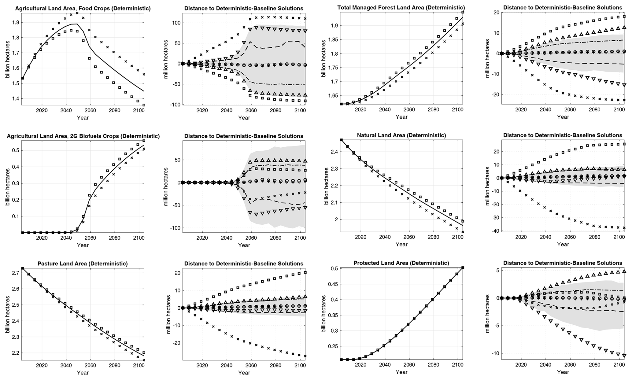
Figure 3Optimal global land use paths. The solid lines represent the deterministic–baseline solutions. Squares represent the deterministic–optimistic solutions or their distances to the deterministic-baseline solutions. Marks represent the deterministic–pessimistic solutions or their distances to the deterministic-baseline solutions. The shaded areas are the ranges of the sample paths' distances to the deterministic-baseline solutions. Pluses represent the average paths, the dashed lines represent the 10 % quantile, circles represent the median paths, and the dashed–dotted lines represent the 90 % quantile. Upward-pointing triangles and downward-pointing triangles represent the distances of the stochastic–optimistic solutions and the stochastic–pessimistic solutions, respectively, to the deterministic-baseline solutions.
We start a discussion of the left-hand side of Fig. 3, which shows the optimal land use paths under perfect foresight. Given the methodological scope of the paper, we will cover these results briefly. Interested readers should refer to Steinbuks and Hertel (2016) for a more detailed analysis of the perfect foresight model.
Beginning with the description of the baseline scenario, we see that, in the first half of the coming century, the area dedicated to food crops increases, peaking around mid-century and declining significantly thereafter (part 1, top panel) as population growth declines while crop production and food processing technologies improve. Consistent with the literature on 2G biofuel deployment potential (National Research Council, 2011), absent aggressive GHG regulations, and biofuel policies, land allocation for second-generation biofuels remains close to zero until the second half of the coming century (part 1, mid panel). It then becomes viable as fossil fuels become scarce and the costs of producing second-generation biofuels decline. This results in greater land requirements for second-generation biofuel crops. As substitution of pasture land for animal feed in livestock production increases (Taheripour et al., 2013), global pasture area declines while managed forest area increases throughout the entire century (part 1, bottom panel, and part 2, top panel). Finally, unmanaged forest areas decline in response to greater requirements for agricultural land (part 2, mid panel), while protected forest areas will more than double by the end of the coming century in light of strong growth in the demand for ecosystem services (part 2, bottom panel). The other two scenarios exhibit broadly similar dynamics.
We now turn to our main findings about the impacts of uncertainty in the crop productivity index on the distribution of global land resources depicted on the right-hand side of Fig. 3. Compared to deterministic scenarios, this uncertainty results in the additional redistribution of land resources to offset the impact of potentially lower yields. The key reason behind this finding is that social preferences exhibit relative risk aversion (Arrow, 1965; Pratt, 1964) in this stochastic application of the FABLE model. Owing to risk aversion and high adjustment costs of future land conversion, some redistribution takes place as a precautionary policy, even in the absence of actual changes in the states of climate or technology. This is a well-known theoretical result in environmental economics literature (Tsur and Zemel, 2014). Compared to the deterministic baseline scenario, the median (i.e., the 50 % quantile) path of global land use that corresponds to the medium state of climate () and the medium technological state () foresees a smaller use of land for food crops (part 1, top panel) and greater use of land for 2G biofuel crops (part 1, mid panel), managed forests (part 2, top panel), and protected land resources (part 2, bottom panel). The differences between stochastic and deterministic paths are small and economically insignificant for all other land resources. This is because land conversion costs of agricultural land for other types of land become larger in the presence of uncertainty. These other types of land have higher adjustment costs of conversion associated with additional time costs of regrowing lumber and livestock and irreversibilities in accessing protected land areas. Land rotation between food crops and 2G biofuel crops is less costly in the FABLE model. This result is consistent with earlier studies that find that closer integration with the energy sector offers greater potential for food–energy substitution and thus also a greater resilience against adverse climate conditions affecting food crop yields (Diffenbaugh et al., 2012; Verma et al., 2014).
While the direction of the effect of the uncertainty in the crop productivity on land conversion can be inferred from the economic theory of environmental and natural resource management under uncertainty (see, e.g., Tsur and Zemel, 2014, and references therein), the extent to which this uncertainty propagates into land conversion depends critically on chosen model structure and parameters. For example, Alexander et al. (2017, p. 1) find that even in the absence of intrinsic uncertainty, “systematic differences in land cover areas are associated with the characteristics modeling approach are at least as great as the differences attributed to scenario variations”. Depending on the assumptions on the substitution of land for other resources, the size of technological progress, and the responsiveness of demand for land-based goods and services to changes in crop productivity, this magnitude can be substantially different from other land use models. However, as we see in Fig. 3, for the same model parameters, the range of land conversion is considerably smaller for the dynamic stochastic model compared to the deterministic scenario analysis. Unlike deterministic analysis, where the solutions paths always stay on a known good or bad trajectory, stochastic analysis allows for future states not to stay in their “best” or “worst” stage. Consequently, optimal land conversion decisions in the stochastic application of the FABLE model are less extreme.
Turning to a specific example, we see from Fig. 3a the difference between the most extreme paths of the stochastic crop productivity index is about 160 million ha by 2100 or about 11 % of the total agricultural area dedicated to food crops. Much of that variation can be attributed to the most extreme (i.e., falling beyond 10th and above 90th percent quantiles) realizations of crop productivity. In line with the argument above, this is because the climate and technological states affecting crop yields are reversible in the stochastic model (that is, if the current state is bad (or good), it could be good (or bad) in the future).
Compared with the deterministic model under the pessimistic (or optimistic) scenario, the social optimum in the stochastic model requires a smaller (or greater) conversion of other types of land to cropland. This is because when the current state of the crop technology index is the worst (best), its future states cannot be worse (better) and have a nonzero probability of being better (worse). The expected future yields will then be better (worse) than the deterministic–pessimistic (optimistic) scenario. As the size of expected crop yields affects the magnitude of the land conversion decisions, the range of stochastic model solutions for agricultural land will be smaller than the range between the most extreme deterministic model solutions. Note this result may not hold if the model solution space is unbounded. This concern does not apply to the stochastic FABLE model because (i) the model’s time horizon is finite, (ii) the crop technology shocks are discrete and finite (hence bounded) based on scientific projections used for the model’s calibration, (iii) all of the model’s state variables (land and fossil fuel resources) are bounded because the total land and the total fossil fuel resources are finite, and (iv) we impose bounds on model decision variables based on the theory of economic dynamics (Barro and Sala-i Martin, 2004), such as strictly positive and finite consumption and output of land-based goods and services; land conversion cannot exceed the total supply of land. The solution space, therefore, must also be bounded because the extent of movement of optimal land uses in any direction is limited by the constraints mentioned above.
Thus, the agricultural land area in the deterministic pessimistic (or optimistic) scenario is larger (or smaller) than the largest (or the smallest) path in the stochastic simulations. For example, in 2100, under the deterministic–pessimistic scenario, the cropland deviation from the deterministic-baseline scenario is about 110 million ha, which is 30 % larger than the largest deviation under the stochastic simulations and more than half of the deviation above the 90 % quantile of the stochastic crop technology index. This result (along with similar results for other land types) demonstrates that scenario analysis can significantly overstate the magnitude of expected agricultural land conversion under uncertain crop yields.
5.2 Optimal path of land-based goods and services under crop yield uncertainty
We now turn to the discussion of optimal paths of land-based goods and services (Fig. 4), keeping the same presentation structure as in the previous section. Deterministic model scenarios (shown on the left-hand side panels of Fig. 4) for land-based goods and services largely mimic trajectories of associated land resources. Specifically, we see steady increases in the production of food crops (part 1, top panel), including livestock and biofuel feedstock, peaking around mid-century and moderating thereafter as consumers satiate their food requirements and the technology of food marketing and processing improves. By 2100, crop production for the livestock feed levels off and even begins to decline. Production of both first- and second-generation biofuels grows as oil becomes more scarce along the baseline path and agricultural yields increase (part 1, mid and bottom panels). Along that optimal path, first-generation biofuels never become a large source of energy consumption, while the production of second-generation biofuels takes off sharply and expands rapidly after 2040 as they become cost-competitive relative to increasingly costly fossil fuels. Production of livestock increases throughout the coming century (part 2, top panel), reflecting shifting diets and the growing demand for processed meat as population income increases (Foley et al., 2011). Production of timber also expands with the growing demand for timber products and further improvements in forest yields (part 2, mid panel). Finally, the consumption of ecosystem services increases throughout most of the coming century as the demand for ecosystem services increases and more natural forest lands become institutionally protected (part 2, bottom panel).
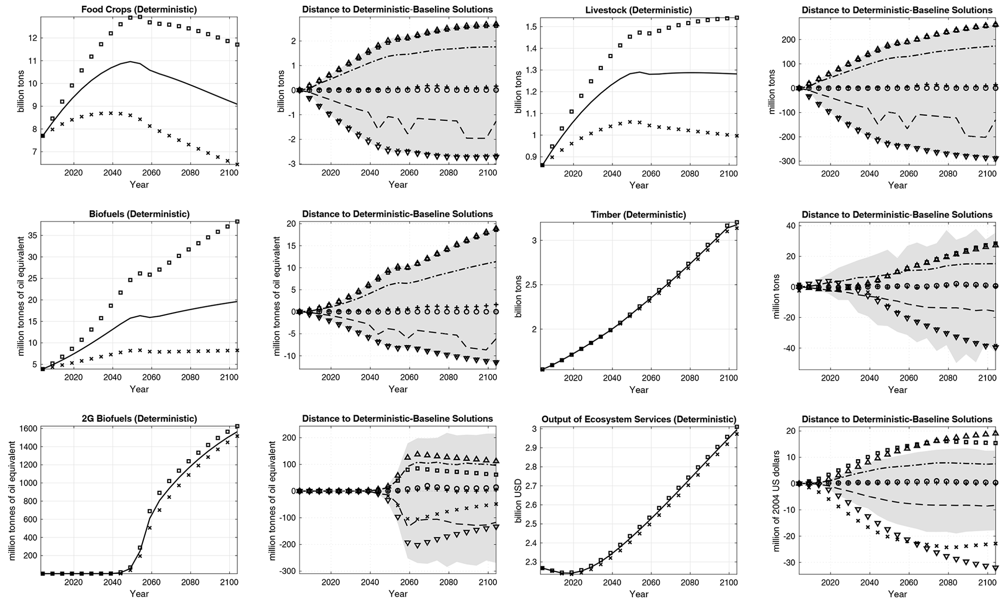
Figure 4Optimal paths of land-based goods and services. The solid lines represent the deterministic–baseline solutions. Squares represent the deterministic–optimistic solutions or their distances to the deterministic-baseline solutions. Marks represent the deterministic–pessimistic solutions or their distances to the deterministic-baseline solutions. The shaded areas are the ranges of the sample paths' distances to the deterministic-baseline solutions. Pluses represent the average paths, the dashed lines represent the 10 % quantile, circles represent the median paths, and the dashed–dotted lines represent the 90 % quantile. Upward-pointing triangles and downward-pointing triangles represent the distances of the stochastic–optimistic solutions and the stochastic–pessimistic solutions, respectively, to the deterministic-baseline solutions.
The results of the dynamic stochastic model simulations (shown on the right-hand side panels of Fig. 4) show that uncertainty in the crop productivity index has a profound effect on the optimal consumption paths of food crops, biofuels, and livestock and a much smaller effect on consumption paths of merchantable timber and ecosystem services. This result is not very surprising, as crop productivity does not directly affect the production of timber and ecosystem services, whereas indirect land use change effects are relatively small in this stochastic application of the FABLE model. Observe that, unlike land use paths, consumption of land-based goods and services is a decision rather than a state variable, and therefore, there are no significant differences between deterministic and stochastic consumption paths.
Focusing on the larger impacts, we see that between the most extreme paths of the stochastic crop productivity index, the production of food crops varies by about 5.3 billion t along both deterministic and stochastic policy paths. This is a sizable change, which suggests a significant variation in levels of consumption in 2100 along different paths of the stochastic crop productivity index. In the FABLE model, much of the variation in the optimal path of food crops comes on the demand side, with the crop productivity decline resulting primarily in the reduced consumption of processed crops and livestock.11 As shown above, the uncertainty-induced supply response is relatively small along the extensive margin in the dynamic stochastic model (i.e., land conversion). In the Appendix (Fig. A2a), we show that the supply response on the intensive margin is smaller, with the ratio of fertilizers to cropland increasing by fewer than 6 kg ha−1 (or 8 %) under extreme realizations of climate and technology uncertainties. About half of that variation corresponds to the most extreme (i.e., falling beyond 10th and above 90th percent quantiles) realizations of crop productivity. This result indicates that extreme uncertainty in crop productivity could have a significant impact on food consumption over the coming century.
Uncertainty in food crop yields has important implications for the production of the first-generation biofuels that are directly affected by both climate and technology states of food crop yields. The difference between the best and worst states of the crop productivity index is about 31 million tonnes of oil equivalent (Mtoe), which exceeds their expected baseline production in 2100. Although climate and technology states of food crop yields do not directly affect yields of the second-generation biofuel crops, production of second-generation biofuels is nonetheless affected through indirect substitution effects of food for energy in the FABLE demand system. There is a sizable variation in the production of second-generation biofuels between extreme paths of the stochastic crop productivity index, which accounts for 450 Mtoe, or about 30 %, of their total production in 2100.
Given the important contribution of livestock feed in the production of livestock, we can see its production is smaller in the pessimistic scenario and larger in the optimistic scenario. The difference in livestock production between the optimistic and pessimistic scenarios accounts for about 550 million t. As the significance of animal feed in livestock production grows over time, the effect of uncertain crop yields becomes more pronounced. Similar to the result for food crops, the most extreme paths of crop productivity account for about a third of all variation in livestock production.
This paper shows the effects of uncertainties associated with nonstationary biophysical processes and technological change on the optimal allocation of natural resources in the long run. In doing so, it applies SCEQ, a cutting-edge computational method for solving nonstationary dynamic high-dimensional stochastic problems, to FABLE, a multi-sectoral dynamic model of global land use.
The study focuses on uncertainty in future crop yields, one of the core uncertainties affecting the evolution of global land use in the long run. Combining scenarios from global climate models and high-resolution output from spatial crop-simulation models for four major crops, it comes up with a plausible range of realizations of climate shocks and their effect on future crop yields. These estimates are supplemented with an extensive survey of recent agro-economic and biophysical studies assessing the potential for closing yield gaps, as well as attaining further advances in potential yields through plant breeding.
The paper's key insight is to illustrate the magnitude of optimal land conversion decisions in the context of different realizations of stochastic crop productivity. Consistent with the economic theory of natural resource management under uncertainty, the agricultural productivity shocks from either adverse climate impacts or unexpected limits on further technological progress result in additional conversion of scarce land resources to offset the impact of potentially lower yields. Owing to intertemporal substitution, some of that conversion takes place even in the absence of actual realization of the climate shocks or technology outcomes. This expansion is accompanied by changes in the consumption of processed food, livestock, and biofuel- and land-based products most affected by changes in crop productivity.
The chosen model (FABLE) seeks to balance computational complexity and economic tractability. Similar to other dynamic economic models, it assumes a bounded solution space, excluding unrealistic scenarios of infinitely low or high crop productivity. It also ignores many features that are standard in more advanced computational land and other resource-use models. Future research should focus on integrating economic decisions under uncertainty into large dynamic natural resource models that feature spatial disaggregation at the regional or zonal level, a more extensive representation of the energy sector, and different types of resources and their production derivatives. Another promising research direction would be to incorporate a more detailed representation of uncertain states backed by an econometric analysis that recovers underlying distributions of uncertain natural resource drivers over time.
This section describes key elements of the FABLE model, as well as its equations, variables, and model parameters. For a full description of the model, including details on model baseline calibration and extensive sensitivity analysis, please refer to Hertel et al. (2016) and Steinbuks and Hertel (2016) and technical appendices therein.
A1 Primary resources
Primary resources comprise land, liquid fossil fuels, and other primary inputs, e.g., labor and capital. The supply of land is fixed and faces competing uses that are determined endogenously by the model. The flow of liquid fossil fuels evolves endogenously along their optimal path, accounting for exogenous discoveries in new fossil fuel reserves. The endowment of other primary inputs is exogenous and evolves along the prespecified global economy growth path.
A1.1 Land
The total land endowment in the model, Ltotal, is fixed. It belongs to a global planner, which fully redistributes land rents back to consumers of land use goods and services. For each period of time t there are four profiles of land in the economy. They include unmanaged forest land, LN, agricultural land, LA, pasture land, LP, and commercially managed forest land, LC. The agricultural land area can be allocated for the cultivation of food crops (denoted LA,c), and second-generation biofuel feedstocks (denoted LA,b2). We assume that the natural forest land consists of two types. Institutionally protected land, LR, includes natural parks, biodiversity reserves, and other types of protected forests. This land is used to produce ecosystem services for society and cannot be converted to commercial land. Unmanaged natural land, LN, can be accessed and either converted to managed land or to protected natural land. Once the natural land is converted to managed land, its potential to yield ecosystem services is diminished. This potential can be partially restored for managed forests with significant land rehabilitation costs incurred. The use of managed land can be shifted between cropland, forestland, and pasture land (see Fig. 1 for a graphical representation of these transitions). We denote land transition flows from land type i to land type j as Δi,j (a negative value means a transition from land type j to land type i). Equations describing the allocation of land across time and different uses are as follows:
Equations (A1) and (A2) define, respectively, the composition of total land and agricultural land in the economy. Equations (A3)–(A5) describe the transitions for unmanaged land, agricultural land, and pasture land.12 Equation (A6) shows the growth path of protected natural land.
Accessing the natural lands comes at a cost associated with building roads and other infrastructure (Golub et al., 2009). In addition, converting natural land to reserved land entails additional costs associated with passing legislation to create new natural parks. We denote the natural land access, rehabilitation, and protection costs as and , respectively. There are also costs of switching between the cropland and the pasture land, denoted as CA,P. We assume that all these costs are continuous, monotonically increasing, and strictly convex functions of converted land. Since we are not aware of empirical studies estimating the magnitudes of long-term adjustment costs in land conversion problems, we choose to calibrate these parameters to match historical land conversion patterns. There are no additional costs of natural land conversion to commercial land, as the revenues from deforestation offset these costs.
Managed forests are characterized by vmax vintages of tree species with vintage ages . At the end of period t, each hectare of managed forest land, has an average density of tree vintage age v, with the initial allocation given and denoted by . The forest rotation ages and management are endogenously determined. Each period the managed forest land can be either planted, harvested, or left to mature. The newly planted trees occupy ΔC,C hectares of land and reach the average age of the first tree vintage next period. The harvested area of tree vintage age v occupies hectares of forest land. The difference between the harvested area of all tree vintage ages and the newly planted area is used for cropland, i.e.,
The following equations describe land use of managed forests:
Equation (A7) describes the composition of managed forest area across vintages. Equation (A8) illustrates the harvesting dynamics of forest areas with the ages and vmax. Equation (A10) shows the transition from the planted area to new forest vintage area.
The average harvesting and planting costs per hectare of new forest planted, co,H and are invariant to scale and are the same across all vintages. Harvesting managed forests and conversion of harvested forest land to agricultural land is subject to additional near-term adjustment costs, cH. The specific functional forms of land conversion costs are shown in Appendix C and Eqs. (C32)–(C37).
Thus, we have defined the vector of land state variables,
and its associated transition laws.
A1.2 Fossil fuels
The initial stock of liquid fossil fuels, XF, is exogenous, and each period of time t adds a new number of fossil fuels, which reflects exogenous technological progress in fossil fuel exploration. This technological progress comprises of both discoveries on new exploitable oil and gas fields, as well as development of new technologies for extraction of non-conventional fossil fuels. The economy extracts fossil fuels, which have two competing uses in our partial-equilibrium model of land use. A part of the extracted fossil fuels, , is converted to fertilizers that are further used in the agricultural sector. The remaining number of fossil fuels, is combusted to satisfy the demand for energy services. The following equation describes supply of fossil fuels:
The cost of fossil fuels, cF, reflects the expenditures for fossil fuel extraction, refining, transportation, and distribution, as well the costs associated with emissions control (e.g., Pigouvian taxes) in the non-land-based economy. We assume that the cost of fossil fuels is a nonlinear quadratic function with accelerating costs as the stock of fossil fuels depletes (Nordhaus and Boyer, 2000):
where the parameter captures the curvature of the liquid fossil fuel cost function.
A1.3 Other primary resources
The initial endowment of all other primary resources in the non-land-based economy, such as labor, physical and human capital, and material inputs, XO, is exogenous in this model. We assume that the growth rate of all other primary resources is a weighted average of the population growth, which reflects demographic changes, and the physical capital growth, κo,X. The following equation describes the supply of other primary inputs:
where Πt is the economy's population, and αo,l is the share of population growth to the growth rate of all other primary resources. Other primary inputs can be used for the production of land-based goods and services or be converted to final goods and services in the non-land economy. The production costs incurred using these inputs are exogenous and have an “iceberg” representation; i.e., they are subtracted from the gross output of land-based goods and services. Thus, state variables for resources other than land are defined as
As XO is exogenous and deterministic, it is a degenerated state variable and not counted as a state variable for model solution purposes.
A2 Intermediate inputs
We analyze six intermediate inputs used in the production of land-based goods and services: petroleum products, fertilizers, crops, biofuels, and raw timber. Fossil fuels are refined and converted to either petroleum products, xp, that are further combusted or to fertilizers, xn, that are used to boost yields in the agricultural sector. Agricultural land and fertilizers are combined to grow food crops, xc or 2G biofuel crops, xc,b2. Food crops can be further converted into processed food and 1G biofuels, xb1, or used as an animal feed, xc,l. 2G biofuel crops can only be converted into 2G biofuels, xb2. 1G biofuels substitute imperfectly for liquid fossil fuels in final energy demand, whereas 2G biofuels and liquid fossil fuels are the perfect substitutes The food crops used as animal feed and pasture land are combined to produce raw livestock, xl. Harvesting managed forests yields raw timber, xw, that is further used in timber processing. The production functions for intermediate inputs can be illustrated by the following equations
where represents that either or is an argument of gj, similarly for and . The specific functional forms of gj(⋅) are shown in Appendix C and Eqs. (C13)–(C21).
A3 Final goods and services
We consider five per capita land-based services that are consumed in the final demand: services from processed crops, yf, livestock, yl, energy, ye, timber, yw, and ecosystem services, yr. Processed crops, livestock, and timber are, respectively, products of food crops, raw livestock, and timber processing. The production of energy services combines liquid fossil fuels with biofuels, and the resulting mix is further combusted. The ecosystem services are the public good to society, which captures recreation, biodiversity, and other environmental goods and services. To close the demand system, we also include other goods and services, yo, which comprise the consumption of other primary inputs not spent on the production of land-based goods and services. We have defined all state variables for the deterministic model:
and the vector of decision variables
where and . The production functions for final per capita land-based goods and services can be illustrated by the following equation:
where some arguments in could be redundant. It follows from Eq. (A15) that the production of final goods and services involves the combination of land resources and intermediate inputs. The specific functional forms of are shown in Appendix C and Eqs. (C22)–(C27), which are functions of L and {xj}. All these equations constitute a part of the feasibility constraint at∈𝒟t(St).
The production of intermediate inputs or final land-based goods and services i incurs costs, co,i, that are subtracted from other available primary resources. The remaining number of other primary resources is converted into other goods and services, which are subsequently consumed in the final demand. As the focus of this model is on the utilization of land-based resources, we introduce the other goods and services, yo, in a very simplified manner. We introduce no additional cost of producing other goods and services, assuming that it is reflected in the size of the endowment of other primary inputs. The specific functional form for yo is shown in Appendix C, Eq. (C26).
A4 Preferences
The economy's per capita utility, u, is derived from the per capita consumption of processed crops, livestock, timber, energy and ecosystem services, and other goods and services. Following the macroeconomic literature, we assume constant relative risk-aversion utility,
where y is the per capita consumption bundle of goods and services, 𝒞(y) is a nonlinear aggregator over y, and γ is the coefficient of relative risk aversion, which captures the economy's attitude to uncertain events. We choose a non-homothetic AIDADS preference (Rimmer and Powell, 1996) to compute 𝒞(y) implicitly:
where α, β, and are positive parameters with . These preferences place greater value on ecosystem services and smaller value on additional consumption of food, energy, and timber products as society becomes wealthier. When γ=1, our utility function is equivalent to the AIDADS utility.
A5 Welfare
We denote the transition laws of land, in Eqs. (A3)–(A6) and Eqs. (A8)–(A10), as
and the transition laws for other resources, in Eqs. (A11)–(A13), as
Combining Eqs. (A18) and (A19), we have
for the deterministic model in the notations of Sect. 2.
The objective of the planner is to maximize the total expected welfare, which is the cumulative expected utility (i.e., a sum of utilities in each state weighted by the probability of each state in a given period) of the population's consumption of final goods and services, y, discounted at the constant rate The planner allocates managed agricultural, pasture, and forest lands for crop, livestock, and timber production, the scarce fossil fuels, and protected natural forests to solve the following problem:
subject to the transition laws (A20) and the feasibility constraints,
which include Eqs. (A15), (C22)–(C27), (C26), and (A17) and nonnegativity constraints for the variables. Here,
is the utility function in the notations of Sect. 4.
B1 Uncertainty in agricultural technology
Advances in crop technology are very difficult to predict due to four interconnected factors (Fischer et al., 2011). First, there is significant uncertainty about the potential for exploiting large and economically significant yield gaps (i.e., the differences between observed and potential crop yields) in developing countries, especially those in sub-Saharan Africa. A second and closely related point is that it is unclear how fast available yield-enhancing technologies can be adopted at a global scale. Third, there is a significant variation in developing countries' institutions and policies that make markets work better and provide a conducive environment for agricultural technology adoption. Finally, while plant breeders continue to make steady gains in further advancing crop yields, progress depends on the level of funding provided for agricultural research. This has proven to be somewhat volatile, with per capita funding falling in the decades leading up to the recent food crisis (Alston and Pardey, 2014). Food prices have risen since 2007, which has stimulated new investments. However, whether this interest will be sustained remains to be seen. Overall, progress from conventional breeding is becoming more difficult. Transgenic (genetic modification) technologies have a proven record of more than a decade of safe and environmentally sound use and thus offer huge potential to address critical biotic and abiotic stresses in the developing world. However, expected yield gains, costs of further developing these technologies, and the political acceptance of genetically modified foods are all highly uncertain.
To quantify the extent to which the advances in crop technology can further boost agricultural yields over the next century, we first need to assess the magnitude of existing yield gaps at the global scale. In a comprehensive study, Lobell et al. (2009) report a significant variation in the ratios of actual to potential yields for major food crops across the world, ranging from 0.16 for tropical lowland maize in sub-Saharan Africa to 0.95 for wheat in Haryana, India. For the purposes of this study, we employ the results of Licker et al. (2010), who conduct comprehensive yield gap analysis using a global crop dataset of harvested areas and yields for 175 crops on a 0.5° geographic grid of the planet for the year 2000. Using these estimates, we calculate the global yield gap as the grid-level output-weighted yield gap of the four most important food crops (wheat, maize, soybeans, and rice). The resulting estimate suggests that average yields are 53 % of potential yields, which is close to the median estimates by Lobell et al. (2009). As a further robustness check, we employ the Decision Support System for Agrotechnology Transfer (DSSAT) crop-simulation model (Jones et al., 2003), run globally on a 0.5° grid in the parallel System for Integrating Impacts Models and Sectors (pSIMS; Elliott et al., 2014b) to simulate yields of the same four major food crops under the best agricultural management conditions and compare simulated yields to their observed yields. The resulting yield gap estimates were not substantially different.
In the optimistic (i.e., good) state of advances in crop technology, we assume that yields will continue to grow linearly throughout the coming century, eliminating the yield gap by 2100. This high-yield scenario rests on the assumption of continued strong growth in investment in agricultural research and development, widespread acceptance of genetically modified crops, continuing institutional reforms in developing countries, and public and private investments in the dissemination of new technologies. The erosion of any one of these component assumptions will likely result in a slowing of crop technology improvements. And there are some grounds for pessimism. In a comprehensive statistical analysis of historical crop production trends, Grassini et al. (2013) note that
despite the increase in investment in agricultural R&D and education … the relative rate of yield gain for the major food crops has decreased over time together with evidence of upper yield plateaus in some of the most productive domains. For example, investment in R&D in agriculture in China has increased threefold from 1981 to 2000. However, rates of increase in crop yields in China have remained constant in wheat, decreased by 64 % in maize as a relative rate and are negligible in rice. Likewise, despite a 58 % increase in investment in agricultural R&D in the United States from 1981 to 2000 (sum of public and private sectors), the rate of maize yield gain has remained strongly linear.
To capture the possibility of much slower technological improvement in the coming century, we specify two more pessimistic scenarios. In the medium state of technology, rather than closing the yield gap by 2100, average yields in 2100 are just three-quarters of yield potential at that point in time. In the bad state of technology, there is no technological progress, and the crop yields stay the same as at the beginning of the coming century. This is the path on which we begin the simulation in 2004. As previously noted, we then specify probabilities with which the crop technology index evolves across the different states of technology.
B2 Uncertainty in climate change impacts
In addition to crop technology uncertainty, there is great uncertainty about the physical environment in which this technology will be deployed. In particular, long-run changes in temperature and precipitation are likely to have an important impact on land productivity in agriculture (IPCC, 2014) and, therefore, the global pattern of land use. Quantification of the impact of climate change on agricultural yields requires coming to grips with three interconnected factors (Alexandratos, 2011). First, there is significant uncertainty in future GHG concentrations along the long-run growth path of the global economy. Second, the general circulation models (GCMs) developed by climate scientists to translate these uncertain GHG concentrations into climate outcomes disagree about the spatially disaggregated deviations of temperature and precipitation from baseline levels. Finally, there is significant uncertainty in the biophysical models used to determine how changes in temperature and precipitation will affect plant growth and the productivity of agriculture in different agroecological conditions. The impact of climate change on food crop yields depends critically on their phenological development, which, in turn, depends on the accumulation of heat units, typically measured as growing degree days (GDDs). More rapid accumulation of GDDs due to climate change speeds up phenological development, thereby shortening key growth stages, such as the grain-filling stage, hence reducing potential yields (Long, 1991). However, rising concentrations of CO2 in the atmosphere result in an increase in potential yields due to improved water use efficiency, often dubbed the “CO2 fertilization effect” (Long et al., 2006). Sorting out the relative importance of these effects and achieving greater confidence in evaluations of climate impacts on agricultural yields remains an important research question in the agronomic literature (Cassman et al., 2010; Rosenzweig et al., 2014).
To quantify the uncertainty in climate impacts on agricultural yields, we use ISIMIP fast-track crop-simulation model data (Rosenzweig et al., 2014). Specifically, we obtain results of four crop-simulation models: GEPIC (Liu et al., 2007), LPJmL (Bondeau et al., 2007), pDSSAT (Jones et al., 2003), and PEGASUS (Deryng et al., 2011). All models are run globally on a 0.5° grid over the period between 1971 and 2099 and weighted by the output of four major food crops (maize, soybeans, wheat, and rice). Since the FABLE model is not spatially explicit, we further aggregate gridded crop yields at a global scale using weights of the size of the aggregate crop output per grid cell. To ensure the simulation results' comparability with the structural parameters of the FABLE model, all models are run under the Representative Concentration Pathway 6.0 W m−2 (RCP6) GHG forcing scenario (Moss et al., 2008). We also consider alternative assumptions on CO2 fertilization effects. Observe that our results are based on four crop-simulation models, though Rosenzweig et al. (2014) consider seven crop-simulation models. The remaining three models have fewer crops and/or temporal frames for model baseline and are thus omitted. Rosenzweig et al. (2014) find that five models, including GEPIC, LPJmL, and pDSSAT models considered in this analysis, yield broadly similar predictions. One model (LPJ–GUESS) not covered here has much higher variation in predicted crop yields under different climate scenarios. Our results may, therefore, understate the range of uncertainty in the climate change impacts on potential crop yields.
To quantify uncertainty in temperature increases due to climate change, we employ outputs for five global climate models (GCMs): GFDL-ESM2M (Dunne et al., 2013), HadGEM2-ES (Collins et al., 2008), IPSL-CM5A-LR (Dufresne et al., 2013), MIROC-ESM-CHEM (Watanabe et al., 2011), and NorESM1-M (Bentsen et al., 2013). For each of the simulations, we fit a linear trend to parsimoniously characterize the evolution of crop yields in the face of climate change over the coming century.
Figure C1 summarizes simulation results for four crop-simulation models and five climate models (with and without fertilization effects) in 2100, normalized relative to assumed yield potential in the absence of climate change. There is significant heterogeneity in terms of both direction and magnitude of climate impacts on agricultural yields across global climate models when the CO2 fertilization effect is considered.13 Regardless of the chosen climate model, for the scenario with fertilization effects, two out of four crop-simulation models (LPJmL and pDSSAT) predict a moderate increase in potential yields (5 %–15 %), whereas the PEGASUS model predicts a large decline in potential yields (20 %–30 %). The GEPIC model predicts that on average crop yields will be little changed, showing a small increase in crop yields for some climate models and a small decline for other models. The predictions of LPJmL and pDSSAT models are reversed when CO2 fertilization effects are removed, showing a decline of about 10 %–15 % in potential yields. The PEGASUS model predicts an even larger decline in potential yields (30 %–35 %), whereas the predictions of GEPIC model show a moderate decline of about 5 %–10 % in potential yields.
Given a large variation in model predictions, we construct five states for potential crop yields under uncertain climate change. These states correspond to quintiles of the distribution of different model outcomes for potential crop yields by 2100. Under two optimistic states of the world, we observe a 2 % and 15 % increases in potential crop yields relative to the model baseline, whereby significant CO2 fertilization effects offset the negative effects of climate change. For the next two states, we see 15 % and 19 % declines in potential crop yields relative to model baseline, whereby CO2 fertilization effects are either small or nonexistent, and the negative effects of climate change tend to prevail. Finally, under the most pessimistic states of the world, drastic adverse effects of climate change combined with the absence of any CO2 fertilization effects result in a 36 % decline in potential crop yields relative to the model baseline.
B3 Transition probabilities
The five possible values of the climate state J1,t are , , , , and , and its probability transition matrix is
where represents the probability from the jth value of J1,t to the ith value for . The three possible values of the technological state J2,t are , , and , and its probability transition matrix is
where represents the probability from the jth value of J2,t to the ith value for . We assume that J2,t is independent of J1,t.
B4 Model
After we add the risks, the state vector becomes
where . And J is a Markov chain, so it can be represented as , where ϵt is a vector of shocks with zero means. The problem is
subject to
and at∈𝒟t(St) representing the feasibility constraints, that is, inequality constraints and the equations other than the above transition laws. The above transition laws are just a special case of
in the notations of Sect. A2 of this Appendix, so we can implement the SCEQ method to solve the dynamic stochastic programming problem. Since our time of interest is years, we change the problem (B1) to have a finite horizon with T=400 years, as a larger T has little impact on our solution in the first 100 years.
In the step 2 of Algorithm 1 for the solution at time s, we replace ϵt by its zero mean to have ; that is, . But this is only for simplicity in notations. In fact, since J is a Markov chain, we replace Jt by its mean conditional on the realized value of Js (i.e., its certainty equivalent approximation):
for all t≥s, where , , , and are two-column vectors representing probability distributions of J1,t and J2,t conditional on the realized values of J1,s and J2,s, respectively. If the realized values of J1,s and J2,s are 𝒥1,i and 𝒥2,j, respectively, then we have and , where is a length 5 column vector, with 1 at the ith element and 0 everywhere else, and is a length 3 column vector, with 1 at the jth element and 0 everywhere else.
C1 Equations
C1.1 Land use
C1.2 Fossil fuels
C1.3 Other primary resources
C1.4 Intermediate products
C1.5 Final goods and services
C1.6 Technology (deterministic)
C1.7 Technology (stochastic)
C1.8 Costs
C1.9 Preferences
C1.10 Population
C1.11 Welfare
with , , and
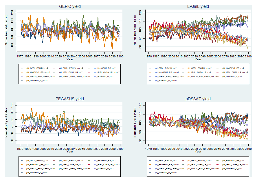
Figure C1Changes in potential crop yields under Representative Concentration Pathway (RCP) 6 scenario in 2100.
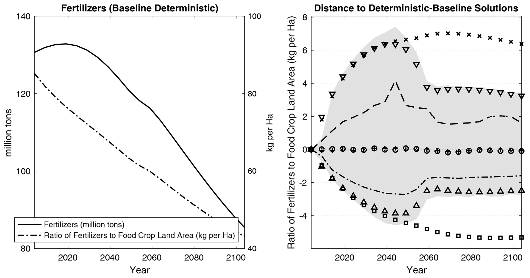
Figure C2Consumption of fertilizers and biofuels. The solid lines represent the deterministic–baseline solutions. Squares represent the deterministic–optimistic solutions or their distances to the deterministic-baseline solutions. Marks represent the deterministic–pessimistic solutions or their distances to the deterministic-baseline solutions. The shaded areas are the ranges of the sample paths' distances to the deterministic-baseline solutions. Pluses represent the average paths, the dashed lines represent the 10 % quantile, circles represent the median paths, and the dashed–dotted lines represent the 90 % quantile. Upward-pointing triangles and downward-pointing triangles represent the distances of the stochastic–optimistic solutions and the stochastic–pessimistic solutions, respectively, to the deterministic-baseline solutions.
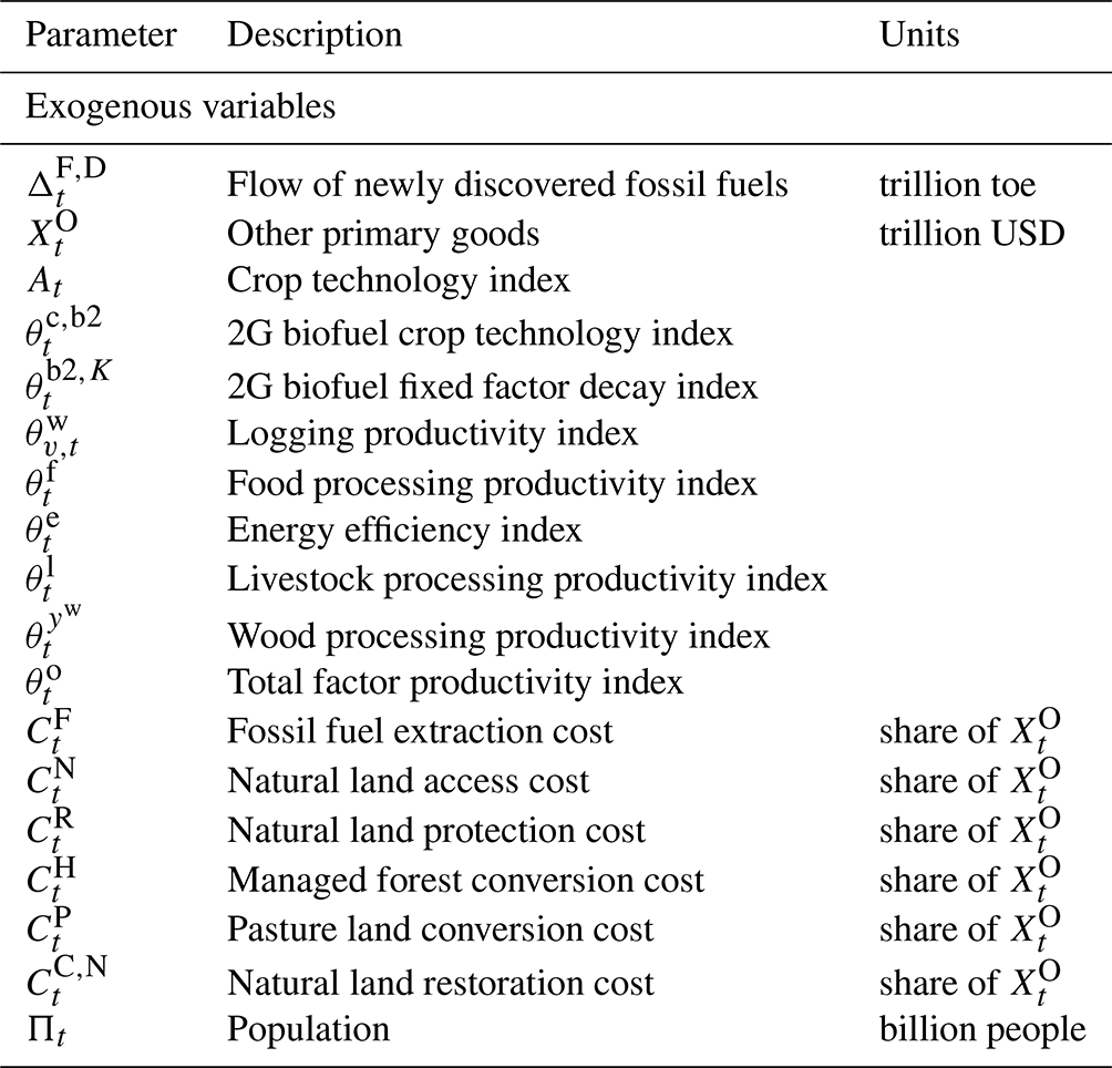
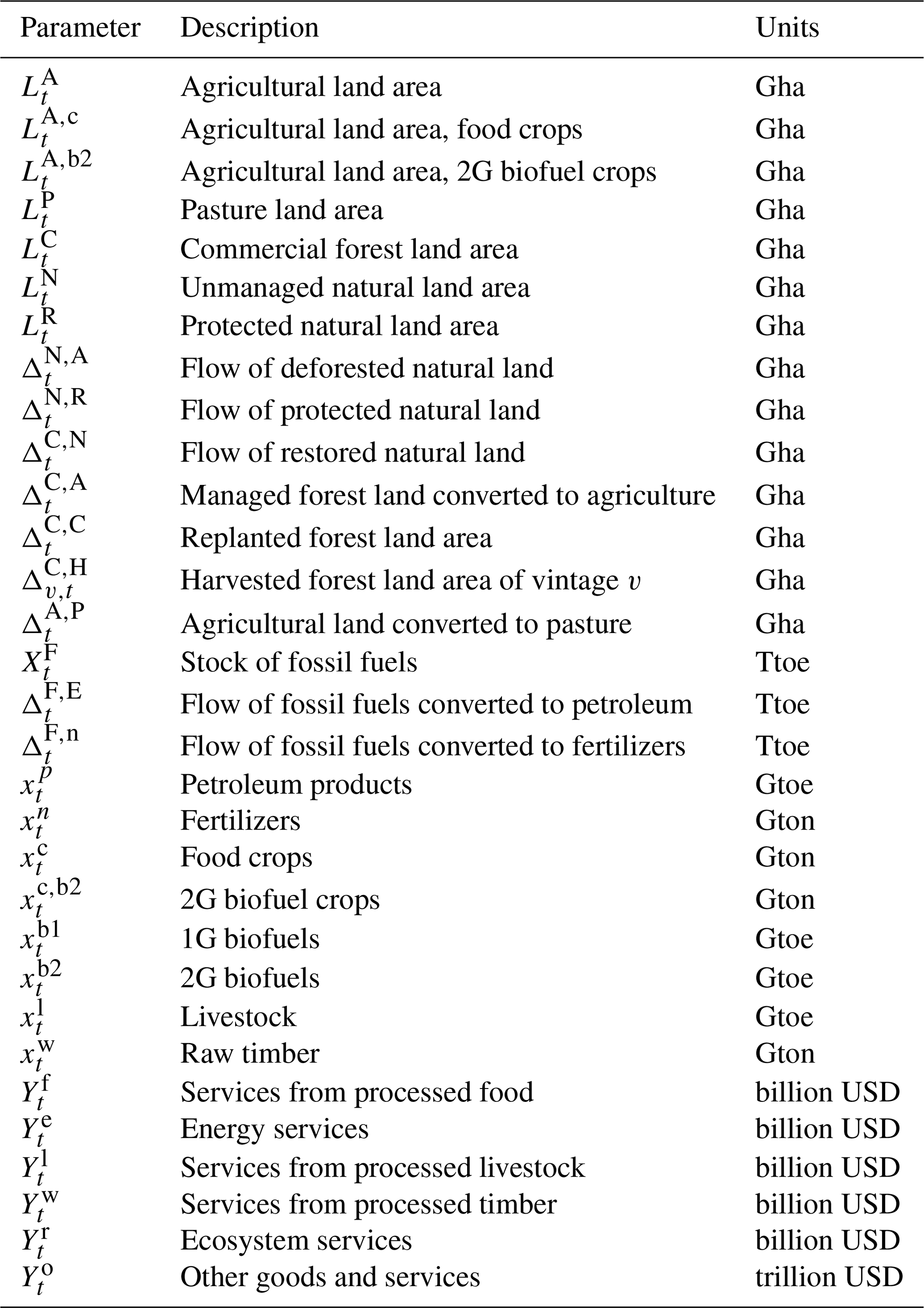
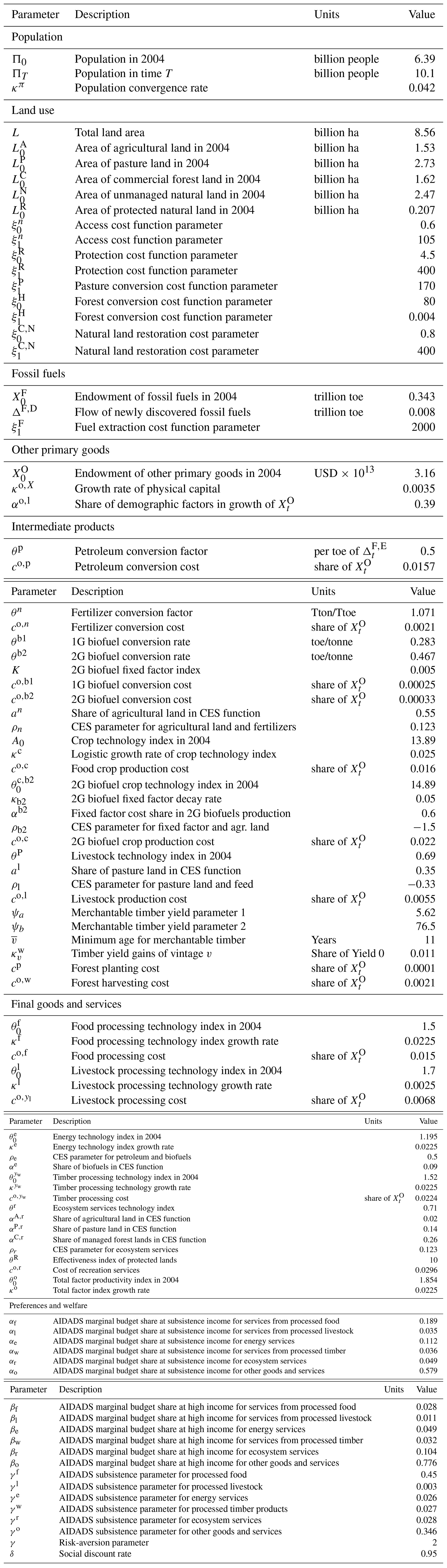
Numerical implementation of the FABLE model and the SCEQ method in the GAMS modeling language is available at https://github.com/jsteinbuks/stfable (last access: 18 April 2024) and https://doi.org/10.5281/zenodo.10014997 (Steinbuks, 2023). The FABLE model is calibrated based on the Global Trade Analysis Project (GTAP) land use database and publicly available data sources. Calibration details are available in the Appendix. The uncertainty in climate impacts on agricultural yields is estimated based on the results of Rosenzweig et al. (2014). Calibration details are available in the Appendix.
JS and YC were the lead contributors to the paper. JS and TWH developed and calibrated the FABLE model. YC developed the SCEQ algorithm and numerically implemented it to assess uncertainty in climate and technology impacts quantitatively. JJ and JS estimated the uncertainty in climate impacts on global crop yields.
The contact author has declared that none of the authors has any competing interests.
Publisher's note: Copernicus Publications remains neutral with regard to jurisdictional claims made in the text, published maps, institutional affiliations, or any other geographical representation in this paper. While Copernicus Publications makes every effort to include appropriate place names, the final responsibility lies with the authors.
Yongyang Cai would like to thank the Becker Friedman Institute at the University of Chicago and Hoover Institution at Stanford University for their support. This paper originates from Cai et al. (2020), which has been separated into this paper and another methodological paper describing the SCEQ computational algorithm.
This research has been supported by the National Science Foundation (grant nos. SES-0951576 and SES-1463644) and the U.S. Department of Agriculture (grant no. 2015-67023-22905).
This paper was edited by Gunnar Luderer and reviewed by Xin Zhao and one anonymous referee.
Alexander, P., Prestele, R., Verburg, P. H., Arneth, A., Baranzelli, C., Batista e Silva, F., Brown, C., Butler, A., Calvin, K., Dendoncker, N., Doelman, J., Dunford, R., Engström, K., Eitelberg, D., Fujimori, S., Harrison, P., Hasegawa, T., Havlik, P., Holzhauer, S., Humpenöder, F., Jacobs-Crisioni, C., Jain, A., Krisztin, T., Page, K., Lavalle, C., Lenton, T., Liu, J., Meiyappan, P., Popp, A., Powell, T., Sands, R., Schaldach, R., Stehfest, E., Steinbuks, J., Tabeau, A., van Meijl, H., Wise, M., and Rounsevell, M.: Assessing Uncertainties in Land Cover Projections, Glob. Change Biol., 23, 767–781, 2017. a
Alexandratos, N.: Critical Evaluation of Selected Projections, in: Economic Analysis of Land Use in Global Climate Change Policy, edited by: Conforti, P., Food and Agriculture Organization of the United Nations, Rome, 465–508, 2011. a
Alston, J. M. and Pardey, P. G.: Agricultural R&D, Food Prices, Poverty and Malnutrition Redux, Staff Paper P14-01, University of Minnesota, Department of Applied Economics, 2014. a
Arrow, K. J.: Aspects of the Theory of Risk-Bearing, Yrjö Jahnsson Foundation, Helsinki, ISBN 0841020019, 1965. a
Babiker, M., Gurgel, A., Paltsev, S., and Reilly, J.: Forward-looking versus Recursive-dynamic Modeling in Climate Policy Analysis: A Comparison, Econ. Model., 26, 1341–1354, 2009. a
Barbier, E. B., Burgess, J. C., Bishop, J., and Aylward, B.: The Economics of the Tropical Timber Trade, Earthscan, London (UK), ISBN 9780367369941, 1994. a
Barro, R. J. and Sala-i Martin, X.: Economic Growth, MIT Press, ISBN 0-262-02553-1, 2004. a
Bentsen, M., Bethke, I., Debernard, J. B., Iversen, T., Kirkevåg, A., Seland, Ø., Drange, H., Roelandt, C., Seierstad, I. A., Hoose, C., and Kristjánsson, J. E.: The Norwegian Earth System Model, NorESM1-M – Part 1: Description and basic evaluation of the physical climate, Geosci. Model Dev., 6, 687–720, https://doi.org/10.5194/gmd-6-687-2013, 2013. a
Bondeau, A., Smith, P. C., Zaehle, S., Schaphoff, S., Lucht, W., Cramer, W., Gerten, D., Lotze-Campen, H., Müller, C., Reichstein, M., and Smith, B.: Modelling the Role of Agriculture for the 20th Century Global Terrestrial Carbon Balance, Glob. Change Biol., 13, 679–706, 2007. a
Brock, W. A. and Majumdar, M.: Global Asymptotic Stability Results for Multisector Models of Optimal Growth under Uncertainty when Future Utilities are Discounted, J. Econ. Theory, 18, 225–243, 1978. a
Bulte, E., van Soest, D., Van Kooten, G., and Schipper, R.: Forest Conservation in Costa Rica when Nonuse Benefits are Uncertain but Rising, Am. J. Agr. Econ., 84, 150–160, 2002. a
Burke, M. B. and Emerick, K.: Adaptation to Climate Change: Evidence from US Agriculture, Am. Econ. J., 8, 106–140, 2016. a
Cai, Y.: Computational methods in environmental and resource economics, Annu. Rev. Resour. Econ., 11, 59–82, https://doi.org/10.1146/annurev-resource-100518-093841, 2019. a, b, c, d
Cai, Y.: The Role of Uncertainty in Controlling Climate Change, Oxford Research Encyclopedia of Economics and Finance, https://doi.org/10.1093/acrefore/9780190625979.013.573, 2021. a
Cai, Y. and Judd, K.: Shape-preserving Dynamic Programming, Math. Method. Oper. Res., 77, 407–421, 2013. a
Cai, Y. and Judd, K.: Advances in Numerical Dynamic Programming and New Applications, in: Handbook of Computational Economics, edited by: Judd, K. L. and Schmedders, K., Elsevier, ISBN 0444512535, 2014. a, b
Cai, Y. and Judd, K.: A Simple but Powerful Simulated Certainty Equivalent Approximation Method for Dynamic Stochastic Problems, Quant. Econ., 14, 651–687, 2023. a, b, c, d, e, f
Cai, Y. and Lontzek, T.: The Social Cost of Carbon with Economic and Climate Risks, J. Polit. Econ., 127, 2684–2734, 2019. a
Cai, Y., Judd, K., Thain, G., and Wright, S.: Solving Dynamic Programming Problems on a Computational Grid, Comput. Econ., 45, 261–284, 2015. a
Cai, Y., Judd, K., and Steinbuks, J.: A Nonlinear Certainty Equivalent Approximation Method for Dynamic Stochastic Problems, Quant. Econ., 8, 117–147, 2017. a, b, c
Cai, Y., Steinbuks, J., Judd, K. L., Jaegermeyr, J., and Hertel, T. W.: Modeling Uncertainty in Large Natural Resource Allocation Problems, Policy Research Working Paper 9159, The World Bank, 2020. a
Cassman, K., Grassini, P., and van Wart, J.: Crop Yield Potential, Yield Trends, and Global Food Security in a Changing Climate, in: Handbook of Climate Change and Agroecosystems, edited by: Hillel, D. and Rosenzweig, C., Imperial College Press, 37–51, ISBN 9781848169838, 2010. a, b
Cassman, K. G.: Ecological Intensification of Cereal Production Systems: Yield Potential, Soil Quality, and Precision Agriculture, P. Natl. Acad. Sci. USA, 96, 5952–5959, 1999. a
Collins, W., Bellouin, N., Doutriaux-Boucher, M., Gedney, N., Hinton, T., Jones, C., Liddicoat, S., Martin, G., O'Connor, F., Rae, J., Senior, C., Totterdell, I., Woodward, S., T., R., and Kim, J.: Evaluation of the HadGEM2 Model, Hadley Center Tech. Note, 74, 2008. a
Conrad, J.: On the Option Value of Old-growth Forest, Ecol. Econ., 22, 97–102, 1997. a
Conrad, J.: Wilderness: Options to Preserve, Extract, or Develop, Resour. Energy Econ., 22, 205–219, 2000. a
Daigneault, A. J., Miranda, M. J., and Sohngen, B.: Optimal Forest Management with Carbon Sequestration Credits and Endogenous Fire Risk, Land Econ., 86, 155–172, 2010. a
Deryng, D., Sacks, W., Barford, C., and Ramankutty, N.: Simulating the Effects of Climate and Agricultural Management Practices on Global Crop Yield, Global Biogeochem. Cy., 25, https://doi.org/10.1029/2009GB003765, 2011. a
Deryng, D., Elliott, J., Folberth, C., Müller, C., Pugh, T. A., Boote, K. J., Conway, D., Ruane, A. C., Gerten, D., Jones, J. W., Khabarov, N., Olin, S., Schaphoff, S., Schmid, E., Yang, H., and Rosenzweig, C.: Regional Disparities in the Beneficial Effects of Rising CO2 Concentrations on Crop Water Productivity, Nat. Clim. Change, 6, 786, https://doi.org/10.1038/nclimate2995, 2016. a
Diffenbaugh, N. S., Hertel, T. W., Scherer, M., and Verma, M.: Response of Corn Markets to Climate Volatility under Alternative Energy Futures, Nat. Clim. Change, 2, 514, https://doi.org/10.1038/nclimate1491, 2012. a
Drud, A. S.: CONOPT – A Large-Scale GRG Code, ORSA J. Comput., 6, 207–216, https://doi.org/10.1287/ijoc.6.2.207, 1994. a
Dufresne, J.-L., Foujols, M.-A., Denvil, S., Caubel, A., Marti, O., Aumont, O., Balkanski, Y., Bekki, S., Bellenger, H., Benshila, R., Bony, S., Bopp, L., Braconnot, P., Brockmann, P., Cadule, P., Cheruy, F., Codron, F., Cozic, A., Cugnet, D., de Noblet, N., Duvel, J.-P., Ethé, C., Fairhead, L., Fichefet, T., Flavoni, S., Friedlingstein, P., Grandpeix, J.-Y., Guez, L., Guilyardi, E., Hauglustaine, D., Hourdin, F., Idelkadi, A., Ghattas, J., Joussaume, S., Kageyama, M., Krinner, G., Labetoulle, S., Lahellec, A., Lefebvre, M.-P., Lefevre, F., Levy, C., Li, Z. X., Lloyd, J., Lott, F., Madec, G., Mancip, M., Marchand, M., Masson, S., Meurdesoif, Y., Mignot, J., Musat, I., Parouty, S., Polcher, J., Rio, C., Schulz, M., Swingedouw, D., Szopa, S., Talandier, C., Terray, P., Viovy, N., and Vuichard, N.: Climate Change Projections using the IPSL-CM5 Earth System Model: from CMIP3 to CMIP5, Clim. Dynam., 40, 2123–2165 https://doi.org/10.1007/s00382-012-1636-1, 2013. a
Dunne, J. P., John, J. G., Shevliakova, E., Stouffer, R. J., Krasting, J. P., Malyshev, S. L., Milly, P. C. D., Sentman, L. T., Adcroft, A. J., Cooke, W., Dunne, K. A., Griffies, S. M., Hallberg, R. W., Harrison, M. J., Levy, H., Wittenberg, A. T., Phillips, P. J., and Zadeh, N.: GFDL's ESM2 Global Coupled Climate?Carbon Earth System Models. Part II: Carbon System Formulation and Baseline Simulation Characteristics. Climate, 26, 2247–2267, 2013. a
Elliott, J., Deryng, D., Müller, C., Frieler, K., Konzmann, M., Gerten, D., Glotter, M., Flörke, M., Wada, Y., Best, N., Eisner, S., Fekete, B. M., Folberth, C., Foster, I., Gosling, S. N., Haddeland, I., Khabarov, N., Ludwig, F., Masaki, Y., Olin, S., Rosenzweig, C., Ruane, A. C., Satoh, Y., Schmid, E., Stacke, T., Tang, Q., and Wisser, D.: Constraints and Potentials of Future Irrigation Water Availability on Agricultural Production Under Climate Change, P. Natl. Acad. Sci. USA, 111, 3239–3244, 2014a. a
Elliott, J., Kelly, D., Chryssanthacopoulos, J., Glotter, M., Jhunjhnuwala, K., Best, N., Wilde, M., and Foster, I.: The Parallel System for Integrating Impact Models and Sectors (pSIMS), Environ. Modell. Softw., 62, 509–516, https://doi.org/10.1016/j.envsoft.2014.04.008, 2014b. a
Evans, L. and Fischer, R.: Yield Potential: its Definition, Measurement, and Significance, Crop Sci., 39, 1544–1551, 1999. a
Fischer, T., Byerlee, D., and Edmeades, G.: Can Technology Deliver on the Yield Challenge to 2050?, in: Economic Analysis of Land Use in Global Climate Change Policy, edited by: Conforti, P., Food and Agriculture Organization of the United Nations, Rome, 389–462, 2011. a
Foley, J. A., Ramankutty, N., Brauman, K. A., Cassidy, E. S., Gerber, J. S., Johnston, M., Mueller, N. D., O’Connell, C., Ray, D. K., West, P. C., Balzer, C., Bennett, E. M., Carpenter, S. R., Hill, J., Monfreda, C., Polasky, S., Rockström, J., Sheehan, J., Siebert, S., Tilman, D., and Zaks, D. P. M.: Solutions for a Cultivated Planet, Nature, 478, 337–342, 2011. a, b, c
Füssel, H.-M.: An Updated Assessment of the Risks from Climate Change Based on Research Published since the IPCC Fourth Assessment Report, Climatic change, 97, 469, https://doi.org/10.1007/s10584-009-9648-5, 2009. a
Golub, A., Hertel, T., and Sohngen, B.: Land Use Modeling in Recursively-Dynamic GTAP Framework, in: Economic Analysis of Land Use in Global Climate Change Policy, edited by: Hertel, T., Rose, S., and Tol, R., Routledge, 235–278, ISBN 9780415847223, 2009. a
Grassini, P., Eskridge, K. M., and Cassman, K. G.: Distinguishing between Yield Advances and Yield Plateaus in Historical Crop Production Trends, Nat. Commun., 4, https://doi.org/10.1038/ncomms3918, 2013. a, b, c
Hausfather, Z. and Peters, G. P.: Emissions–the “Business as Usual” Story is Misleading, Nature, 577, 618–620, 2020. a
Hertel, T., Steinbuks, J., and Tyner, W.: What is the Social Value of Second Generation Biofuels?, Appl. Econ. Perspect. P., 38, 599–617, 2016. a, b
Hertel, T. W., Steinbuks, J., and Baldos, U.: Competition for Land in the Global Bioeconomy, Agr. Econ., 44, 129–138, 2013. a
IPCC: Climate Change 2014: Impacts, Adaptation and Vulnerability: Contribution of Working Group II to the Fifth Assessment Report of the Intergovernmental Panel on Climate Change, Cambridge University Press, ISBN 1107058163, 2014. a, b
Jägermeyr, J., Gerten, D., Schaphoff, S., Heinke, J., Lucht, W., and Rockström, J.: Integrated Crop Water Management Might Sustainably Halve the Global Food Gap, Environ. Res. Lett., 11, 025002, https://doi.org/10.1088/1748-9326/11/2/025002, 2016. a
Jägermeyr, J., Müller, C., Ruane, A. C., Elliott, J., Balkovic, J., Castillo, O., Faye, B., Foster, I., Folberth, C., Franke, J. A., Fuchs, K., Guarin, J. R., Heinke, J., Hoogenboom, G., Iizumi, T., Jain, A. K., Kelly, D., Khabarov, N., Lange, S., Lin, T.-S., Liu, W., Mialyk, O., Minoli, S., Moyer, E. J., Okada, M., Phillips, M., Porter, C., Rabin, S. S., Scheer, C., Schneider, J. M., Schyns, J. F., Skalsky, R., Smerald, A., Stella, T., Stephens, H., Webber, H., Zabel, F., and Rosenzweig, C.: Climate Impacts on Global Agriculture Emerge Earlier in New Generation of Climate and Crop Models, Nature Food, 2, 873–885, 2021. a
Jones, J. W., Hoogenboom, G., Porter, C., Boote, K., Batchelor, W., Hunt, L., Wilkens, P., Singh, U., Gijsman, A., and Ritchie, J.: The DSSAT Cropping System Model, Eur. J. Agron., 18, 235–265, 2003. a, b
Judd, K. L.: Numerical Methods in Economics, The MIT press, ISBN 9780262547741, 1998. a
Lanz, B., Dietz, S., and Swanson, T.: Global Economic Growth and Agricultural Land Conversion under Uncertain Productivity Improvements in Agriculture, Am. J. Agr. Econ., 100, 545–569, 2017. a, b, c, d
Leroux, A., Martin, V., and Goeschl, T.: Optimal Conservation, Extinction Debt, and the Augmented Quasi-option Value, J. Environ. Econ. Manage., 58, 43–57, 2009. a
Licker, R., Johnston, M., Foley, J. A., Barford, C., Kucharik, C. J., Monfreda, C., and Ramankutty, N.: Mind the Gap: How do Climate and Agricultural Management Explain the “Yield Gap” of Croplands around the World?, Global Ecol. Biogeogr., 19, 769–782, 2010. a, b
Liu, J., Williams, J. R., Zehnder, A. J., and Yang, H.: GEPIC–Modelling Wheat Yield and Crop Water Productivity with High Resolution on a Global Scale, Agr. Syst., 94, 478–493, 2007. a
Lobell, D. B. and Field, C. B.: Global Scale Climate – Crop Yield Relationships and the Impacts of Recent Warming, Environ. Res. Lett., 2, 014002, https://doi.org/10.1088/1748-9326/2/1/014002, 2007. a
Lobell, D. B., Cassman, K. G., and Field, C. B.: Crop Yield Gaps: their Importance, Magnitudes, and Causes, Annu. Rev. Environ. Resour., 34, 179, https://doi.org/10.1146/annurev.environ.041008.093740, 2009. a, b, c
Long, S.: Modification of the Response of Photosynthetic Productivity to Rising Temperature by Atmospheric CO2 Concentrations: Has its Importance been Underestimated?, Plant Cell Environ., 14, 729–739, 1991. a
Long, S. P., Ainsworth, E. A., Leakey, A. D., Nösberger, J., and Ort, D. R.: Food for Thought: Lower-Than-Expected Crop Yield Stimulation with Rising CO2 Concentrations, Science, 312, 1918–1921, 2006. a
Majumdar, M. and Radner, R.: Stationary Optimal Policies with Discounting in a Stochastic Activity Analysis Model, Econometrica, 51, 1821–1837, 1983. a
Miranda, M. J. and Fackler, P. L.: Applied Computational Economics and Finance, MIT press, ISBN 9780262633093, 2004. a, b
Moss, R., Babiker, M., Brinkman, S., Calvo, E., Carter, T., Edmonds, J., Elgizouli, I., Emori, S., Lin, E., Hibbard, K., Jones, R., Kainuma, M., Kelleher, J., Lamarque, J.-F., Manning, M., Matthews, B., Meehl, J., Meyer, L., Mitchell, J., and Zurek, M.: Towards New Scenarios for Analysis of Emissions, Climate Change, Impacts, and Response Strategies, Tech. Rep. PNNL-SA-63186, Pacific Northwest National Laboratory (PNNL), Richland, WA (US), 2008. a, b
National Research Council: Renewable Fuel Standard: Potential Economic and Environmental Effects of U.S. Biofuel Policy, National Academies Press, ISBN 978-0-309-18751-0, 2011. a
Nikas, A., Doukas, H., and Papandreou, A.: A Detailed Overview and Consistent Classification of Climate-Economy Models, in: Understanding Risks and Uncertainties in Energy and Climate Policy, Springer, 1–54, 2019. a
Nordhaus, W. D. and Boyer, J.: Warming the World: Economic Models of Global Warming, MIT press, ISBN 9780262280747, 2000. a
Pindyck, R. S.: Uncertainty in Environmental Economics, Rev. Env. Econ. Policy, 1, 45–65, 2007. a
Pratt, J. W.: Risk Aversion in the Small and in the Large, Econometrica, 32, 122–136, 1964. a
Rimmer, M. and Powell, A.: An Implicitly Additive Demand System, Appl. Econ., 28, 1613–1622, 1996. a, b
Rose, S. K., Ahammad, H., Eickhout, B., Fisher, B., Kurosawa, A., Rao, S., Riahi, K., and van Vuuren, D. P.: Land-based mitigation in climate stabilization, Energy Economics, 34, 365–380, https://doi.org/10.1016/j.eneco.2011.06.004, 2012. a
Rosenzweig, C., Elliott, J., Deryng, D., Ruane, A., Arneth, A., Bootef, K., Folberth, C., Glotter, M., Khabarov, N., Müller, C., Neumann, K., Piontek, F., Pugh, T., Schmid, E., Stehfest, E., and Jones, J.: Assessing Agricultural Risks of Climate Change in the 21st Century in a Global Gridded Crop Model Intercomparison, P. Natl. Acad. Sci. USA, 111, 3268–3273, 2014. a, b, c, d, e, f, g, h
Schmitz, C., van Meijl, H., Kyle, P., Nelson, G. C., Fujimori, S., Gurgel, A., Havlik, P., Heyhoe, E., d’Croz, D. M., Popp, A., Sands, R., Tabeau, A., van der Mensbrugghe, D., von Lampe, M., Wise, M., Blanc, E., Hasegawa, T., Kavallari, A., and Valin, H.: Land-Use Change Trajectories Up to 2050: Insights from a Global Agro-Economic Model Comparison, Agr. Econ., 45, 69–84, 2014. a
Sohngen, B. and Mendelsohn, R.: An Optimal Control Model of Forest Carbon Sequestration, Am. J. Agr. Econ., 85, 448–457, 2003. a
Sohngen, B. and Mendelsohn, R.: A Sensitivity Analysis of Forest Carbon Sequestration, in: Human-Induced Climate Change: An Interdisciplinary Assessment, edited by: Schlesinger, M., Cambridge University Press, 227–237, 2007. a
Steinbuks, J.: Stochastic Implementation of the FABLE model, Zenodo [code], https://doi.org/10.5281/zenodo.10014997, 2023. a
Steinbuks, J. and Hertel, T.: Forest, Agriculture, and Biofuels in a Land use model with Environmental services (FABLE), GTAP Working Paper 71, Center for Global Trade Analysis, Department of Agricultural Economics, Purdue University, 2012. a
Steinbuks, J. and Hertel, T.: Confronting the Food-Energy-Environment Trilemma: Global Land Use in the Long Run, Environ. Resour. Econ., 63, 545–570, 2016. a, b, c, d, e
Steinbuks, J. and Hertel, T. W.: Energy Prices Will Play an Important Role in Determining Global Land Use in the Twenty First Century, Environ. Res. Lett., 8, 014014, https://doi.org/10.1088/1748-9326/8/1/014014, 2013. a, b, c
Stokey, N. L., Lucas, R. E., and Prescott, E. C.: Recursive Methods in Economic Dynamics, Harvard University Press, ISBN 978-0674750968, 1989. a, b
Taheripour, F., Hurt, C., and Tyner, W. E.: Livestock Industry in Transition: Economic, Demographic, and Biofuel Drivers, Animal Frontiers, 3, 38–46, 2013. a
Tian, X., Sohngen, B., Kim, J. B., Ohrel, S., and Cole, J.: Global Climate Change Impacts on Forests and Markets, Environ. Res. Lett., 11, 035011, https://doi.org/10.1088/1748-9326/11/3/035011, 2016. a
Tsionas, E. G. and Kumbhakar, S. C.: Markov Switching Stochastic Frontier Model, Econ. J., 7, 398–425, 2004. a
Tsur, Y. and Zemel, A.: Dynamic and Stochastic Analysis of Environmental and Natural Resources, in: Handbook of Regional Science, edited by: Fischer, M. and Nijkamp, P., Springer-Verlag Berlin Heidelberg, 929–949, ISBN 978-3-642-23429-3, 2014. a, b, c
Verma, M., Hertel, T., and Diffenbaugh, N.: Market-Oriented Ethanol and Corn-Trade Policies can Reduce Climate-Induced US Corn Price Volatility, Environ. Rese. Lett., 9, 064028, https://doi.org/10.1088/1748-9326/9/6/064028, 2014. a
Watanabe, S., Hajima, T., Sudo, K., Nagashima, T., Takemura, T., Okajima, H., Nozawa, T., Kawase, H., Abe, M., Yokohata, T., Ise, T., Sato, H., Kato, E., Takata, K., Emori, S., and Kawamiya, M.: MIROC-ESM 2010: model description and basic results of CMIP5-20c3m experiments, Geosci. Model Dev., 4, 845–872, https://doi.org/10.5194/gmd-4-845-2011, 2011. a
Weitzman, M. L.: What Is The “Damages Function” For Global Warming – And What Difference Might It Make?, Climate Change Economics, 1, 57–69, 2010. a
Zhao, X., Calvin, K. V., Wise, M. A., Patel, P. L., Snyder, A. C., Waldhoff, S. T., Hejazi, M. I., and Edmonds, J. A.: Global Agricultural Responses to Interannual Climate and Biophysical Variability, Environ. Res. Lette., 16, 104037, https://doi.org/10.1088/1748-9326/ac2965, 2021. a, b, c, d
Several recent studies, e.g., Cai and Lontzek (2019), have successfully integrated uncertainty about economic and climate outcomes in a stochastic integrated assessment climate–economy framework. For a review of this related literature, see Cai (2019, 2021).
Climate change will likely affect the productivity of other land resources, such as forestland. Several recent modeling studies (see, e.g., Tian et al., 2016, and references therein) have suggested that climate change is likely to result in higher forest growth and greater timber yields, as well as in more forest dieback, with the net effects varying over time and space. Incorporating these effects is beyond the scope of this study and is left for future research.
This makes them difficult to incorporate into an economic model of land use. Consequently, they have historically been neglected in economic models of global land use change. More recently, these natural lands have been incorporated via location-specific supply curves depicting the potential for bringing these lands into commercial production (e.g., in the REF MAGNET model, https://www.magnet-model.eu/model, last access: 18 April 2024). However, the ecosystem services provided by these lands are not explicitly valued as they are in the FABLE model, where they are explicitly included in the utility function.
In FABLE, bioenergy does not include the potential use of biomass in power generation. This limitation is acknowledged in Steinbuks and Hertel (2016, p. 566): “A more serious limitation to this study is our omission of the potential demand for biomass in power generation. Under some scenarios, authors have shown this to be an important source of feedstock demand by mid-century (Rose et al., 2012). However absent a full representation of the electric power sector, our framework is ill-suited to addressing this issue.”
More recent projections using ensembles of latest-generation crop and climate models find larger uncertainty in climate impacts on major crop yields (Jägermeyr et al., 2021). Unfortunately, these data were not available at the time of the research. Our results should therefore be taken as conservative estimates of the impacts of climate uncertainties in crop yields.
FABLE model baseline assumes no climate regulations and other GHG mitigation measures required to achieve RCP4.5 or lower radiative forcing values, whereas the realism of RCP8.5 as the “business-as-usual” scenario has been questioned by the literature (Hausfather and Peters, 2020).
For notational simplicity, we keep the same mathematical representation of a transition function, even if some of its elements are redundant. For example, if Gt,i is deterministic, we still denote it as even though . Similarly, if there are some unused elements of ϵt or some redundant arguments in a function Gt,j, we can multiply them by zero in Gt,j and thus still use .
As ϵt is a serially uncorrelated stochastic process, we can replace ϵt by its zero mean in the functions of Gt in Eq. (5) if all transition laws are continuous. For problems with a discrete Markov chain in transition laws, we can use the same technique as described in Cai et al. (2017) for NLCEQ with a discrete stochastic state to obtain the corresponding deterministic model (1). That is, given the realization of the Markov chain at time s, we can compute expectations of the Markov chain at all times after s conditional on the value at the time s and then replace the stochastic process by the path of the conditional expectations in step 2 of Algorithm 1.
The model converges to its stationary state around 2150. The differences in land use allocations between 2100 and 2150 are small and, therefore, not reported.
Since the SCEQ algorithm is based on simulation, additional simulations could lead to a wider range, and our current solution could underestimate the range in comparison with the range from all possible simulation paths. The difference will, however, be small and will not affect the economic significance of the main findings.
Demand for land-based goods and services in the FABLE model is governed by the AIDADS (An Implicit, Directly Additive Demand System) designed to encompass consumption behavior across a wide range of incomes (Rimmer and Powell, 1996). This is essential for a dynamic model of the global economy. We have estimated three key parameters for each commodity category – the subsistence level of consumption, the marginal budget share at very low (subsistence) income, and the marginal budget share at very high levels of income. The former two are large for food products. In the FABLE model, baseline households become wealthier, and the marginal budget share for food items and the subsistence share becomes very small, approaching zero for very high incomes. Consequently, households' demand response becomes larger.
Equations (A2) and (A4) do not account for the transition from forestry to pasture land. Throughout the past century, tropical forests, particularly in the Latin America region, have been extensively converted to pasture land (Barbier et al., 1994). However, in the FABLE model, the conversion of forest land to pasture is never optimal, as cropland has higher productivity for cattle breeding at the same conversion (stumpage) cost.
Field trials show that higher atmospheric CO2 concentrations enhance photosynthesis and reduce crop water stress (Deryng et al., 2016). This fertilization effect interacts with other factors such as nutrient availability, and current-generation crop models are characterized by large uncertainties regarding net CO2 fertilization potentials at larger spatial scales. In line with previous studies (Rosenzweig et al., 2014; Elliott et al., 2014a; Jägermeyr et al., 2016), we use a constant CO2 case as a pessimistic assumption regarding climate change effects and a transient CO2 case according to the Representative Concentration Pathways (RCPs) to reflect a more optimistic case.
- Abstract
- Introduction
- Stochastic FABLE model
- Modeling crop yield uncertainty
- Method of model solution: the SCEQ algorithm
- Model results
- Conclusions
- Appendix A: FABLE model description
- Appendix B: Quantifying the uncertainty in crop yields
- Appendix C: Model equations, variables and parameters
- Code and data availability
- Author contributions
- Competing interests
- Disclaimer
- Acknowledgements
- Financial support
- Review statement
- References