mesas.py v1.0: a flexible Python package for modeling solute transport and transit times using StorAge Selection functions

StorAge Selection (SAS) transport theory has recently emerged as a framework for representing material transport through a control volume. It can be seen as a generalization of transit time theories and lumped-parameter models to allow for arbitrary temporal variability in the rate of material flow in and out of the control volume, and in the transport dynamics. SAS is currently the state-of-the-art approach to interpreting tracer transport. Here, we present mesas.py, a Python package implementing the SAS framework. mesas.py allows SAS functions to be specified using several built-in common distributions, as a piecewise linear cumulative distribution function (CDF), or as a weighted sum of any number of such distributions. The distribution parameters and weights used to combine them can be allowed to vary in time, permitting SAS functions of arbitrary complexity to be specified. mesas.py simulates tracer transport using a novel mass-tracking scheme and can account for first-order reactions and fractionation. We present a number of analytical solutions to the governing equations and use these to validate the code. For a benchmark problem the time-step-averaging approach of the mesas.py implementation provides a reduction in mass balance errors of up to 15 times in some cases compared with a previous implementation of SAS.

1 Introduction

StorAge Selection (SAS) is a theoretical framework for modeling transport dynamics through spatially integrated systems (control volumes). It is applicable for any system in which it is reasonable to assume that the bulk material flowing out of the system (at rate Q(t)) at some time t is some conservative mixture of the bulk material that flowed in at earlier times (at rate J(t)). For example, it is often reasonable to assume that the streamflow and evapotranspiration leaving a watershed are some conservative mixture of precipitation that fell on that watershed at earlier times. The conservative bulk material in that case is simply the water comprising the rainfall, streamflow, and evapotranspiration. The development of this theory and related issues in watershed hydrology have been recently reviewed in Benettin et al. (2022).

SAS is a generalization of the idea of a transit time distribution (TTD), which has proven useful in a wide range of disciplines, including chemical engineering (Ross et al., 2006), transportation engineering (Tyworth and Zeng, 1998), groundwater hydrology (Dupas et al., 2020; Rinaldo et al., 2015; Danesh-Yazdi et al., 2018), surface water hydrology (Stockinger et al., 2016; Rodriguez and Klaus, 2019; Rodriguez et al., 2021), medicine (Rossum et al., 1989), and others. However TTDs have previously required that the bulk material flow through the system be approximately steady (i.e., $J\left(t\right)=Q\left(t\right)=$ a constant). SAS relaxes this assumption in a rigorous and general way, so that it can (in principle) be used to characterize transport through any system in which the bulk material flow is conserved. However, to date, SAS functions have not been widely adopted in practice. In part, this is due to the perception that they are too complex and data-hungry.

Our objective here is to provide detailed documentation of mesas.py, a Python implementation of SAS functions that is easy to use, highly flexible, and computationally accurate. This implementation is already the basis of online teaching resources (Harman, 2020), and we hope to develop more in the future. It is essential, therefore, that a peer-reviewed publication exists that supports and documents the software.

In a typical forward-modeling use-case, we wish to predict the concentration C_Q(t) of a conservative tracer in the bulk material outflow Q(t), which is assumed to be a conservative mixture of previous bulk material inflows J(t) in which the tracer concentration was C_J(t). If this is the case, the outflow concentration C_Q(t) will be some weighted average of past values of C_J(t). The transit time distribution p_Q(T,t) gives those weights:

$$\begin{array}{}\text{(1)}& C_Q\left(t\right)=\underset{\mathrm{0}}{\overset{\mathrm{\infty }}{\int }}{C}_J(t-T)p_Q(T,t)\mathrm{d}T.\end{array}$$

SAS provides a means to calculate the time-varying distribution p_Q(T,t) for a given system. An overview of SAS and related approaches can be found in Botter (2012), Harman (2015), Rinaldo et al. (2015), and Benettin and Bertuzzo (2018).

The basic equations required to calculate p_Q(T,t) (discussed in Sect. 2 below) are not especially difficult to solve numerically, but some care is required. An implementation of SAS in MATLAB (tran-SAS) is already available (Benettin and Bertuzzo, 2018). mesas.py replicates the functionality of tran-SAS but offers the following features:

• mesas.py offers an extremely flexible framework for specifying SAS functions, allowing them to be arbitrarily complex and variable in time. This includes the ability to specify SAS functions as a time-varying weighted sum of other functions (Rodriguez and Klaus, 2019) and as a (time-varying) piecewise linear cumulative distribution function (CDF) with any number of segments.

• mesas.py uses a novel mass-tracking approach that estimates solute/tracer mass storage as part of the solution.

• mesas.py estimates the time-step-averaged transit times and mass fluxes using a fourth-order Runge–Kutta method, and it provides superior numerical accuracy and mass balance accounting (as we shall demonstrate).

• mesas.py allows for time-varying first-order reactions and time-varying solute/tracer fractionation.

• mesas.py is implemented in Python and Fortran and is designed to be easy to install (through conda-forge) and user-friendly.

The governing equations of the SAS framework are given in Sect. 2 of this paper, including the novel approach to solute/tracer mass tracking. Calculating the storage and release of solutes/tracers continuously in tandem with calculation of the TTD (rather than using the convolution after the TTD has been obtained) makes incorporating reactions and fractionation into the SAS function simple and intuitive. Section 3 gives details of the code, including the numerical implementation, the method for specifying SAS functions, and procedures for running the code.

In Sect. 4 of the paper, we test the code against a number of benchmarks in the form of analytical solutions to the governing equations. These include cases of steady and unsteady flow. We compare the accuracy of mesas.py against that of tran-SAS for the unsteady-flow case.

2 Governing equations

To estimate p_Q and solve Eq. (1), two key pieces of information are required: (1) time series of inflows J(t) and outflows Q_q(t) (there may be more than one outflow, hence the subscript index q) and (2) SAS functions Ω_q (one for each outflow q) that capture the way each outflow is drawn from the water of different ages available to be removed from storage. The inflow and outflow data are used to solve expressions of conservation of mass that describe how the age distribution of the material in storage changes over time as material is added and removed. The SAS functions are needed to calculate this solution because they characterize the relative rate at which material of different relative ages is selected for removal.

2.1 Conservation laws

2.1.1 Conservation law for the bulk material flows

The bulk flow is the material that makes up the inflows and outflows from the system, carrying tracers and other species of material with it. Typically, in hydrologic applications, the bulk flow is water. As is typical in hydrology, we assume that the water is incompressible so we can refer to units of volume for convenience, but the framework is valid for any conservative bulk flow as long as fluxes, storages, and concentrations are expressed in consistent compatible units.

The conservation equation for the bulk flow can be obtained by considering an incremental volume s_T(T,t) that has an age T at time t; therefore, it entered at time $t_i=t-T$. Note that s_T(T,t) has units of volume (or mass) per time, as it is the amount that entered in an infinitesimal increment of time. If the inflow rate is J(t) at some time in the past t=t_i, then $s_T(\mathrm{0},t)=J\left(t\right)$. Over time, the quantity of bulk flow residing in storage represented by s_T depletes due to outflows. Assuming that outflows are indexed by q, and each has an outflow rate Q_q and transit time distribution p_q(T,t), the time evolution of s_T from some initial time t_i to the present time t is given by the following:

$$\begin{array}{}\text{(2)}& {\displaystyle \frac{\mathrm{d}}{\mathrm{d}t}}{s}_T(t-t_i,t)=J\left(t\right)\mathit{\delta }(t-t_i)-\sum _q{Q}_q\left(t\right)p_q(t-t_i,t),\end{array}$$

where δ(⋅) is the Dirac delta distribution. Typically, the derivative on the left here is broken up into two terms, as follows:

$$\begin{array}{}\text{(3)}& {\displaystyle \frac{\mathrm{d}}{\mathrm{d}t}}{s}_T(t-t_i,t)={\displaystyle \frac{\partial s_T}{\partial t}}+{\displaystyle \frac{\partial s_T}{\partial T}}.\end{array}$$

However, the form given in Eq. (2) serves to remind us that these two derivatives can be thought of as representing the rate at which s_T changes as it simultaneously moves through time and ages. We can think of it moving along a characteristic curve that is a straight line in age–time space, with a slope of one unit of age per unit of time and passing through the point $(T,t)=(\mathrm{0},t_i)$. The computational method of mesas.py is based on numerically integrating along this characteristic curve.

Integrating s_T over all ages up to some age T gives the cumulative form S_T, known as the age-ranked storage:

$$\begin{array}{}\text{(4)}& S_T(T,t)=\underset{\mathrm{0}}{\overset{T}{\int }}{s}_T(\mathit{\tau },t)\mathrm{d}\mathit{\tau }.\end{array}$$

This is the volume of bulk material residing in storage that is younger than T at time t. The bulk material conservation equation is often expressed in terms of this cumulative quantity and P_q(T,t), the cumulative form of p_q(T,t). Equation (2) can be obtained from the cumulative form by taking the derivative with respect to T.

S_T is also essential for solving Eq. (2) through its role in evaluating the SAS function (see Sect. 2.2 below). Therefore, even though the primary state variable that mesas.py solves for is s_T(T,t), the code must also keep track of the accumulating values of S_T(T,t).

2.1.2 Conservation law for solutes

Consider a conservative solute or tracer that travels ideally with the bulk material. We can define m_T(T,t) as the incremental tracer mass that entered at time t_i and is now remaining in storage (m_T). We can also define a notion of age-ranked concentration in storage as the increment of age-ranked solute mass per increment of age-ranked storage:

$$\begin{array}{}\text{(5)}& C_T(T,t)={\displaystyle \frac{m_T(T,t)}{s_T(T,t)}}.\end{array}$$

Note that this is not a concentration in the usual sense. C_T may not correspond to an actual measurable concentration anywhere in the system if materials of different ages have intermingled sufficiently. However, it does (by definition) equal the input concentration C_J(t) just as water enters the system; thus,

$$\begin{array}{}\text{(6)}& m_T(\mathrm{0},t)=C_T(\mathrm{0},t)s_T(\mathrm{0},t)=C_J\left(t\right)J\left(t\right).\end{array}$$

It also gives the effective concentration of the solute in the increment of water at age $T=t-t_i$ that is contributing to each outflow, and thus controls the mass flux out for a given age increment, which we will term ${\dot{m}}_q$:

$$\begin{array}{}\text{(7)}& {\dot{m}}_q(T,t)=Q_q\left(t\right)C_T(T,t)p_q(T,t).\end{array}$$

Putting these together, we can write a conservation law for the solute as follows:

$$\begin{array}{}\text{(8)}& {\displaystyle \frac{\mathrm{d}}{\mathrm{d}t}}{m}_T(t-t_i,t)=J\left(t\right)C_J\left(t\right)\mathit{\delta }(t-t_i)-\sum _q{\dot{m}}_q(t-t_i,t).\end{array}$$

This equation is analogous to Eq. (2), but instead of tracking the bulk material along a characteristic curve in age–time space, it tracks the mass of solute/tracer.

2.1.3 Accounting for fractionation and reactions

We can easily generalize Eq. (8) in two ways. First, we can account for the effect of fractionation in the outflows. Sometimes the concentration of a solute in an outflow is different from its concentration in storage. For example, chloride (which has been used as a tracer in catchment studies, such as Harman, 2015) can leave in discharge, but it is not carried out of the catchment by evapotranspiration. Thus, the effective concentration of chloride in the evaporative flux must be zero. A less extreme example is where stable water isotope ratios in evaporation tend to be lighter than those in the water left behind.

We can account for this fractionation in a simple way by assuming that the concentration of the solute in outflow q is some (possibly time-varying) multiple α_q(t) of the concentration in storage. To accomplish this we modify Eq. (7) to include the following:

$$\begin{array}{}\text{(9)}& {\dot{m}}_q(T,t)={\mathit{\alpha }}_q\left(t\right)Q_q\left(t\right)C_T(T,t)p_q(T,t).\end{array}$$

When α_q=1, there is no fractionation. α_q<1 will result in reduced concentrations in the given outflow, and α_q=0 excludes the solute from the outflow. It is also possible to set α_q>1 if the solute is preferentially entrained in the outflow. Note that if isotope fractionation is being modeled, the isotope data must be given as an isotope ratio, rather than a δ value (per mill). For example, values of δ¹⁸O must be converted using $R={\mathit{\delta }}^{\mathrm{18}}\mathrm{O}/\mathrm{1000}+\mathrm{1}$. The value of α is simply the regular fractionation factor ${\mathit{\alpha }}_{A/B}$ (Kendall and Caldwell, 1998). If fractionation is being neglected, δ values may be used.

Second, we can account for first-order reactions. The change in C_T resulting from mass introduced or removed by such a reaction can be modeled as follows:

$$\begin{array}{}\text{(10)}& {\displaystyle \frac{\mathrm{d}{C}_T}{\mathrm{d}t}}=k_{\mathrm{1}}(C_{\mathrm{eq}}-C_T).\end{array}$$

From this we can define a reaction term ${\dot{m}}_R$ as follows:

$$\begin{array}{}\text{(11)}& \begin{array}{rl}{\dot{m}}_R(T,t)& =s_T(T,t){\displaystyle \frac{d{C}_T}{\mathrm{d}t}}=k_{\mathrm{1}}\left(t\right)\left(C_{\mathrm{eq}}\right(t\left)s_T\right(T,t)\\ & -m_T(T,t)),\end{array}\end{array}$$

where k₁ is a first-order reaction rate and C_eq is an equilibrium concentration (both of which may vary in time).

Including fractionation and the reaction terms in the solute conservation law gives

$$\begin{array}{}\text{(12)}& \begin{array}{rl}{\displaystyle \frac{\mathrm{d}}{\mathrm{d}t}}{m}_T(t-t_i,t)& =J\left(t\right)C_J\left(t\right)\mathit{\delta }(t-t_i)-\sum _q{\dot{m}}_q(T,t)\\ & +{\dot{m}}_R(T,t),\end{array}\end{array}$$

where ${\dot{m}}_q$ is given by Eq. (9) and ${\dot{m}}_R$ is given by Eq. (11).

The actual outflow concentration at time t is obtained by integrating ${\dot{m}}_q(T,t)$ over all ages T≤T_max and then adding the “old-water” contribution:

$$\begin{array}{}\text{(13)}& \begin{array}{rl}{C}_q\left(t\right)& ={\displaystyle \frac{\mathrm{1}}{Q_q\left(t\right)}}\underset{\mathrm{0}}{\overset{T_{\max }}{\int }}{\dot{m}}_q(T,t)\mathrm{d}T+C_{\mathrm{old}}\\ & \times (\mathrm{1}-P_q(T_{\max },t\left)\right),\end{array}\end{array}$$

where C_old is the concentration assigned to all the water in storage with an age greater than T_max. T_max=t usually, but it may be set to be less than t to reduce memory demands or speed up computation (at the cost of potentially truncating the contributions of water that entered early in the simulation to outflows later).

2.2 StorAge Selection (SAS) functions

The equations above cannot be solved on their own, as p_Q is not known. The SAS functions provide the required additional relationship linking the age-ranked storage and the transit time distribution.

Given a volume of age-ranked storage S_T representing all the bulk material in a control volume with an age of T or less, the cumulative SAS function Ω_q is defined as a function that gives the fraction of outflow Q_q drawn from S_T(T,t). This is also (by definition) the fraction of discharge with an age of T or less, which is simply P_q(T,t). Thus, we can write the following:

$$\begin{array}{}\text{(14)}& P_q(T,t)={\mathrm{\Omega }}_q(S_T,t),\end{array}$$

where $S_T=S_T(T,t)$. That is, the SAS function and the cumulative transit time distribution both give the fraction of discharge with age T or less, but the SAS function expresses the age in terms of age-ranked storage S_T(T,t), rather than age T. This has proven to be very useful because P_q(T,t) varies in time due to variations in fluxes, whereas Ω_q(S_T,t) only varies when the manner in which storage turns over varies. In many applications, SAS functions have been approximated by a variety of continuous distributions with good results (Benettin et al., 2022). We will discuss several that have been implemented in mesas.py in the next section.

By taking the derivative of the equation above and applying the chain rule, we can see that

$$\begin{array}{}\text{(15)}& p_q(T,t)={\mathit{\omega }}_q(S_T,t)s_T(T,t),\end{array}$$

where ω_q is the density form of Ω_q. The left-hand side of this equation is the rate of discharge of water with age T. The right-hand side is the rate at which water is removed from the age-ranked storage at S_T(T,t).

The SAS functions needed to represent a particular system are typically obtained by first choosing a functional form from those presented below and then tuning the parameters of that functional form such that the model predictions match the tracer observations. It should be noted that there is currently an element of subjectivity and imprecision here, as multiple functional forms may produce equally acceptable fits to the available data (Harman, 2019). In previous applications to watersheds, streamflow has been represented with a heavily right-skewed distribution whose mean varies inversely with catchment wetness, whereas evapotranspiration (ET) has been represented by uniform distributions over the youngest water in storage. More physically based parameterizations may be available in the future.

2.2.1 Continuous SAS functions available in mesas.py

The SAS function must be specified so that it accurately captures how a system turns over, releasing storage as bulk outflow. At present, three continuous distributions commonly used for specifying SAS functions are available as built-in options in mesas.py: the beta, Kumaraswamy, and gamma distributions. More details on each distribution are given below.

These distributions each have at least two parameters: a location parameter (S_min) and a scale parameter (S₀). These parameters both have units of storage, and they serve to shift and scale the values of S_T into a normalized form:

$$\begin{array}{}\text{(16)}& x={\displaystyle \frac{S_T-S_{\min }}{S_{\mathrm{0}}}}.\end{array}$$

Here, x=0 if S_T<S_min. In mesas.py, the values of S₀, S_min, and all other parameters can be given as constant values, or different values for every time step can be provided.

Briefly, the three aforementioned built-in distributions are as follows:

• Beta distribution. The CDF of the beta distribution is given by

  $$\begin{array}{}\text{(17)}& \begin{array}{rl}& \text{Beta}(S_T;S_{\min },S_{\mathrm{0}},\mathit{\alpha },\mathit{\beta })={\displaystyle \frac{B(x;\mathit{\alpha },\mathit{\beta })}{B(\mathit{\alpha },\mathit{\beta })}}\\ & S_{\min }\le S_T\le S_{\min }+S_{\mathrm{0}},\end{array}\end{array}$$

  where $B(x;\mathit{\alpha },\mathit{\beta })$ and B(α,β) are the incomplete and complete beta functions, and $\mathit{\alpha },\mathit{\beta }>\mathrm{0}$. This distribution has been used to represent the SAS function of systems whose total active storage volume S(t) has been estimated (Benettin et al., 2022). In those cases, S_m is set to zero and S₀=S(t).

• Kumaraswamy distribution. The CDF of the Kumaraswamy distribution is given by

  $$\begin{array}{}\text{(18)}& \begin{array}{rl}& \mathrm{\text{Kumaraswamy}}(S_T;S_{\min },S_{\mathrm{0}},a,b)=\mathrm{1}-(\mathrm{1}-x^a{)}^b\\ & S_{\min }\le S_T\le S_{\min }+S_{\mathrm{0}},\end{array}\end{array}$$

  where $a,b>\mathrm{0}$. This distribution has also been used to represent the SAS function of systems whose total active storage volume has been estimated.

• Gamma distribution. The gamma distribution is given by

  $$\begin{array}{}\text{(19)}& \begin{array}{rl}& \text{Gamma}(S_T;S_{\min },S_{\mathrm{0}},\mathit{\alpha })={\displaystyle \frac{\mathrm{\Gamma }(\mathit{\alpha },x)}{\mathrm{\Gamma }\left(\mathit{\alpha }\right)}}\\ & \text{for}{S}_{\min }\le S_T<\mathrm{\infty }.\end{array}\end{array}$$

  This distribution has been used to represent the SAS function of systems whose total volume is unknown, and the right tail of the SAS function is assumed to taper exponentially for sufficiently large S_T (Harman, 2015; Benettin et al., 2022).

In addition, any distribution specified by the scipy.stats library can be used in mesas.py by converting its CDF into a piecewise linear form (see next section). This is done automatically within mesas.py. The accuracy of the results obtained this way may be poor. The piecewise linear form may be inaccurate where the PDF changes rapidly (as a gamma distribution does near S_T=0 when α<1) or where it approaches an asymptotic value at the tails.

2.2.2 Piecewise linear SAS functions in mesas.py

SAS functions can also be specified as a piecewise linear CDF with N segments. When N=1, this is simply a uniform distribution. These linear segments join control points $(S_{Tq,\mathrm{0}},{\mathrm{\Omega }}_{q,\mathrm{0}}),(S_{Tq,\mathrm{1}},{\mathrm{\Omega }}_{q,\mathrm{1}})\mathrm{\dots }(S_{Tq,N},{\mathrm{\Omega }}_{q,N})$. To ensure that the result is a probability distribution, we require $\mathrm{0}={\mathrm{\Omega }}_{q,\mathrm{0}}\le {\mathrm{\Omega }}_{q,\mathrm{1}}\le \mathrm{\dots }\le {\mathrm{\Omega }}_{q,N}=\mathrm{1}$ and $\mathrm{0}\le S_{Tq,\mathrm{0}}\le S_{Tq,\mathrm{1}}\le \mathrm{\dots }\le S_{Tq,N}$. The SAS function is specified by giving these control points, which may vary in time. The PDF ω_q(S_T,t) is piecewise constant:

$$\begin{array}{}\text{(20)}& {\displaystyle }{\mathit{\omega }}_q(S_T,t)=\left\{\begin{array}{ll}\frac{{\mathrm{\Omega }}_{q,\mathrm{1}}-{\mathrm{\Omega }}_{q,\mathrm{0}}}{S_{Tq,\mathrm{1}}-S_{Tq,\mathrm{0}}}& S_{Tq,\mathrm{0}}\le S_T<S_{Tq,\mathrm{1}}\\ \frac{{\mathrm{\Omega }}_{q,\mathrm{2}}-{\mathrm{\Omega }}_{q,\mathrm{1}}}{S_{Tq,\mathrm{2}}-S_{Tq,\mathrm{1}}}& S_{Tq,\mathrm{1}}\le S_T<S_{Tq,\mathrm{2}}\\ \mathrm{\cdots }& \\ \frac{{\mathrm{\Omega }}_{q,N}-{\mathrm{\Omega }}_{q,N-\mathrm{1}}}{S_{Tq,N}-S_{Tq,N-\mathrm{1}}}& S_{Tq,N-\mathrm{1}}\le S_T<S_{Tq,N}\\ \mathrm{0}& \text{otherwise}.\end{array}\right.\end{array}$$

The parameters of the N-segment piecewise SAS function are the N+1 values of S_T q,n and the N−1 values of Ω_q,n (recall that ${\mathrm{\Omega }}_{q,\mathrm{0}}=\mathrm{0}$ and ${\mathrm{\Omega }}_{q,N}=\mathrm{1}$).

2.2.3 SAS functions built from weighted sums of components

mesas.py also allows an SAS function to be specified as a (time-varying) weighted sum of component SAS functions, each of which may specified in any of the available ways. This approach was first suggested by Rodriguez and Klaus (2019), and Wilusz et al. (2020) provided evidence supporting its validity.

Given M component SAS functions (indexed by m) defined using one of the methods presented above, the overall SAS function can be obtained as follows:

$$\begin{array}{}\text{(21)}& {\mathit{\omega }}_q(S_T,t)=\sum _{m=\mathrm{1}}^M{f}_{q,m}\left(t\right){\mathit{\omega }}_{q,m}(S_T,t),\end{array}$$

where f_q,m(t) is a (possibly time-varying) weight. These weights must be provided as inputs to the model. The weights should sum to 1 at each time step (although this is not enforced by mesas.py).

3 Methods

3.1 Numerical implementation

The numerical implementation of the governing equations in mesas.py is reminiscent of a numerical finite-volume scheme. We will assume that time steps Δt and age steps ΔT are equal.

First, age-step-averaged forms of the state variables are obtained by integrating in T over an interval of past input times $[t_i-\mathrm{\Delta }T,t_i]$:

$$\begin{array}{}\text{(22)}& {\displaystyle }{s}_i\left(t\right)={\displaystyle \frac{\mathrm{1}}{\mathrm{\Delta }T}}\underset{t_i-\mathrm{\Delta }T}{\overset{t_i}{\int }}{s}_T(t-\mathit{\tau },t)\mathrm{d}\mathit{\tau },\text{(23)}& {\displaystyle }{m}_i\left(t\right)={\displaystyle \frac{\mathrm{1}}{\mathrm{\Delta }T}}\underset{t_i-\mathrm{\Delta }T}{\overset{t_i}{\int }}{m}_T(t-\mathit{\tau },t)\mathrm{d}\mathit{\tau }.\end{array}$$

For notational consistency, we can define the cumulative version of this as S_i(t), but it is precisely equal to $S_T(t-t_i,t)$. We can use these to write age-step-averaged forms of Eqs. (2) and (12), respectively:

$$\begin{array}{}\text{(24)}& \begin{array}{rl}\mathrm{\Delta }T{\displaystyle \frac{\mathrm{d}{s}_i}{\mathrm{d}t}}& =J\left(t\right)\underset{t_i-\mathrm{\Delta }T}{\overset{t_i}{\int }}\mathit{\delta }(t-\mathit{\tau })\mathrm{d}\mathit{\tau }-\sum _q{Q}_q\left(t\right)\\ & \underset{t_i-\mathrm{\Delta }T}{\overset{t_i}{\int }}{p}_q(t-\mathit{\tau },t)\mathrm{d}\mathit{\tau },\end{array}\end{array}$$

$$\begin{array}{}\text{(25)}& {\displaystyle }\begin{array}{rl}\mathrm{\Delta }T{\displaystyle \frac{\mathrm{d}{m}_i}{\mathrm{d}t}}& =J\left(t\right)C_J\left(t\right)\underset{t_i-\mathrm{\Delta }T}{\overset{t_i}{\int }}\mathit{\delta }(t-\mathit{\tau })\mathrm{d}\mathit{\tau }\\ & -\sum _q\left(\underset{t_i-\mathrm{\Delta }T}{\overset{t_i}{\int }}{\dot{m}}_q(t-\mathit{\tau },t)\mathrm{d}\mathit{\tau }\right)\\ & -\underset{t_i-\mathrm{\Delta }T}{\overset{t_i}{\int }}{\dot{m}}_R(t-\mathit{\tau },t)\mathrm{d}\mathit{\tau }.\end{array}\end{array}$$

There are a few things to unpack here. First, note that, due to the properties of the Dirac δ-function, the integral ${\int }_{t_i-\mathrm{\Delta }T}^{t_i}\mathit{\delta }(t-\mathit{\tau })\mathrm{d}\mathit{\tau }$ is 1 if $t_i-\mathrm{\Delta }T<t<t_i$ but is 0 otherwise. Thus, for all times after t_i, the first term disappears in both equations above. This behavior can be represented using the indicator function ${\mathbf{\text{1}}}_{[t_i-\mathrm{\Delta }T,t_i)}\left(t\right)$, which we will write as 1_i(t) for short.

The age-step-averaged TTD p_qi(t) can be expressed in terms of the cumulative TTD, and thus in terms of the SAS function, as follows:

$$\begin{array}{}\text{(26)}& \begin{array}{rl}{p}_{qi}\left(t\right)\mathrm{\Delta }T& =\underset{t_i-\mathrm{\Delta }T}{\overset{t_i}{\int }}{p}_q(t-\mathit{\tau },t)\mathrm{d}\mathit{\tau }=P_q(t-t_i+\mathrm{\Delta }T,t)\\ & -P_q(t-t_i,t)\\ & ={\mathrm{\Omega }}_q\left(S_T\right(t-(t_i-\mathrm{\Delta }T),t),t)\\ & -{\mathrm{\Omega }}_q\left(S_T\right(t-t_i,t),t)\\ & ={\mathrm{\Omega }}_q\left(S_i\right(t)+s_i(t),t)-{\mathrm{\Omega }}_q\left(S_i\right(t),t).\end{array}\end{array}$$

The time-step-averaged values of ${\dot{m}}_q$ and ${\dot{m}}_R$ can then be obtained if we are willing to approximate that the age-ranked concentration C_T is constant over the interval ΔT at $C_T=m_i/s_i$. This amounts to approximating the concentration C_J in the corresponding input bulk material as constant over this interval.

Thus, we can express the governing equations as the set of ordinary differential equations (ODEs):

$$\begin{array}{}\text{(27)}& {\displaystyle }\begin{array}{rl}\mathrm{\Delta }T{\displaystyle \frac{\mathrm{d}{s}_i}{\mathrm{d}t}}& =J\left(t\right){\mathbf{1}}_i\left(t\right)-\sum _q{Q}_q\left(t\right)p_{qi}\left(t\right)\mathrm{\Delta }T\\ & =f_s(s_i,S_i,t)\mathrm{\Delta }T,\end{array}\text{(28)}& {\displaystyle }\begin{array}{rl}\mathrm{\Delta }T{\displaystyle \frac{\mathrm{d}{m}_i}{\mathrm{d}t}}& =J\left(t\right)C_J\left(t\right){\mathbf{1}}_i\left(t\right)-{\displaystyle \frac{m_i\left(t\right)}{s_i\left(t\right)}}\\ & \left(\sum _q{\mathit{\alpha }}_q\left(t\right)Q_q\left(t\right)p_{qi}\left(t\right)\mathrm{\Delta }T\right)\\ & -k_{\mathrm{1}}\left(t\right)\left(C_{\mathrm{eq}}\right(t\left)s_i\right(t)-m_i(t\left)\right)\\ & =f_m(m_i,s_i,S_i,t)\mathrm{\Delta }T.\end{array}\end{array}$$

If the right-hand side of these equations were functions of the state variables s_i and m_i and a number of time-variable coefficients (J, Q_q, C_J, α_q, k₁, and C_eq), these would be ODEs. The dependence of the SAS function on the cumulative value S_i(t) complicates matters only slightly.

The numerical solution of these equations involves two core tasks:

1. estimating the rates of change $f_s(s_i,S_i,t)$ and $f_m(m_i,s_i,S_i,t)$ and

2. using these to estimate the state variables s_i and m_i (and S_i) at a future time.

Let us assume t=jΔt and T=iΔT, and recall that age and time steps are equal in size. Now define ${\mathtt{s}}_{\mathtt{i}}^{\mathtt{j}}=s_i\left(j\mathrm{\Delta }t\right)$, and define ${\mathtt{m}}_{\mathtt{i}}^{\mathtt{j}}$ similarly. Particular care must be taken to ensure that an accurate value of S_T is used to evaluate the SAS function. Let

$$\begin{array}{}\text{(29)}& {\mathtt{S}}_{\mathtt{i}}^{\mathtt{j}}=\sum _{k=i+\mathrm{1}}^j{\mathtt{s}}_{\mathtt{k}}^{\mathtt{j}}\mathrm{\Delta }t.\end{array}$$

Note that, by this definition, the value of ${\mathtt{S}}_{\mathtt{i}}^{\mathtt{j}}$ depends on ${\mathtt{s}}_{\mathtt{i}+\mathtt{1}}^{\mathtt{j}}$ but not on ${\mathtt{s}}_{\mathtt{i}}^{\mathtt{j}}$. For the fourth-order Runge–Kutta (RK4) and midpoint methods, the state variables must be evaluated at an intermediate point halfway between the regular time steps. The value of ${\mathtt{S}}_{\mathtt{i}}^{\mathtt{j}+\frac{\mathtt{1}}{\mathtt{2}}}$ can be estimated as follows:

$$\begin{array}{}\text{(30)}& {\mathtt{S}}_{\mathtt{i}}^{\mathtt{j}+\frac{\mathtt{1}}{\mathtt{2}}}={\displaystyle \frac{{\mathtt{S}}_{\mathtt{i}}^{\mathtt{j}}+{\mathtt{S}}_{\mathtt{i}}^{\mathtt{j}+\mathtt{1}}}{\mathrm{2}}}.\end{array}$$

However, note that ${\mathtt{S}}_{\mathtt{i}}^{\mathtt{j}+\mathtt{1}}$ can be found only after an estimate of ${\mathtt{s}}_{\mathtt{i}+\mathtt{1}}^{\mathtt{j}+\mathtt{1}}$ is obtained. This suggests that, in order to calculate how ${\mathtt{s}}_{\mathtt{i}}^{\mathtt{j}}$ becomes ${\mathtt{s}}_{\mathtt{i}}^{\mathtt{j}+\mathtt{1}}$, we must first have determined both ${\mathtt{s}}_{\mathtt{i}+\mathtt{1}}^{\mathtt{j}}$ and ${\mathtt{s}}_{\mathtt{i}+\mathtt{1}}^{\mathtt{j}+\mathtt{1}}$. In other words, for an accurate numerical solution, we need to know the fate of younger material before we can determine the fate of older material. Because of this, mesas.py solves $j\to j+\mathrm{1}$ for all i before moving on to i+1, and so on.

By default, mesas.py uses the RK4 method to estimate the value of ${\mathtt{s}}_{\mathtt{i}}^{\mathtt{j}+\mathtt{1}}$ as follows:

$$\begin{array}{}\text{(31)}& \begin{array}{rl}{k}_{\mathrm{1}}& =f_s\left({\mathtt{s}}_{\mathtt{i}}^{\mathtt{j}},{\mathtt{S}}_{\mathtt{i}}^{\mathtt{j}},j\mathrm{\Delta }t\right),\\ k_{\mathrm{2}}& =f_s\left({\mathtt{s}}_{\mathtt{i}}^{\mathtt{j}}+\frac{\mathrm{1}}{\mathrm{2}}{k}_{\mathrm{1}}\mathrm{\Delta }t,{\mathtt{S}}_{\mathtt{i}}^{\mathtt{j}+\frac{\mathtt{1}}{\mathtt{2}}},\left(j+\frac{\mathrm{1}}{\mathrm{2}}\right)\mathrm{\Delta }t\right),\\ k_{\mathrm{3}}& =f_s\left({\mathtt{s}}_{\mathtt{i}}^{\mathtt{j}}+\frac{\mathrm{1}}{\mathrm{2}}{k}_{\mathrm{2}}\mathrm{\Delta }t,{\mathtt{S}}_{\mathtt{i}}^{\mathtt{j}+\frac{\mathtt{1}}{\mathtt{2}}},\left(j+\frac{\mathrm{1}}{\mathrm{2}}\right)\mathrm{\Delta }t\right),\\ k_{\mathrm{4}}& =f_s\left({\mathtt{s}}_{\mathtt{i}}^{\mathtt{j}}+k_{\mathrm{3}}\mathrm{\Delta }t,{\mathtt{S}}_{\mathtt{i}}^{\mathtt{j}+\mathtt{1}},\left(j+\mathrm{1}\right)\mathrm{\Delta }t\right),\\ k_{*}& ={\displaystyle \frac{k_{\mathrm{1}}+\mathrm{2}{k}_{\mathrm{2}}+\mathrm{2}{k}_{\mathrm{2}}+k_{\mathrm{1}}}{\mathrm{6}}},\\ {\mathtt{s}}_{\mathtt{i}}^{\mathtt{j}+\mathtt{1}}& ={\mathtt{s}}_{\mathtt{i}}^{\mathtt{j}}+k_{*}\mathrm{\Delta }t.\end{array}\end{array}$$

Similar steps are followed to estimate ${\mathtt{m}}_{\mathtt{i}}^{\mathtt{j}+\mathtt{1}}$ using $f_m(m_i,s_i,S_i,t)$. During the calculation, the intermediate values of p_q, ${\dot{m}}_q$, and ${\dot{m}}_R$ are also tracked and time-step-averaged according to the same scheme. It is also possible to run mesas.py with a midpoint method or with a forward Euler scheme, although at some sacrifice in terms of numerical accuracy.

The state variables are held in memory in arrays whose columns are times and whose rows are ages. Thus, stepping through time steps j for a fixed input time i corresponds to stepping along a diagonal of a state variable matrix.

mesas.py allows initial conditions to be specified for the age-ranked storage s_T and solute mass m_T. This is useful for restarting calculations or spinning up the simulation. The initial conditions are supplied as a vector of values ${\mathtt{s}}_{\mathtt{k}}^{\mathtt{0}}$ and ${\mathtt{m}}_{\mathtt{k}}^{\mathtt{0}}$ for ages k. Each entry represents the value of s_T and m_T at t=0 averaged over each age interval and is used to populate the first column of the matrices holding the state variables.

mesas.py proceeds by solving all the time steps $j\to j+\mathrm{1}$ for the first age step before moving on to second, and so forth. Typically, when there are N time steps, the solution is found for N age steps also. This is sometimes excessive because the contributions of bulk flow from the start of the simulation to the final time step may be negligible. The number of age steps can also be larger than N, although this will only have value if an initial condition is provided that gives values of ${\mathtt{s}}_{\mathtt{i}}^{\mathtt{0}}$ for more than >N ages. Note that all outflow with an unknown age is assigned concentration C_old.

3.2 Model specification and input structure

Inputs to mesas.py come in two main forms:

1. parameters specifying the SAS function(s), solute properties, and other model settings and

2. time series of inflows, outflows, and other variables.

The parameters are specified using a nested data structure that can be stored and read from a JSON-formatted text file or fed into a model object instance directly as a Python dictionary. The time series can be provided as a .csv text file or as a pandas data frame.

The parameter data structure consists of a dictionary of key:value pairs, where a “key” is an immutable label (typically a string) and a “value” is an object that can be retrieved from the dictionary using the associated key. The values can themselves be dictionaries, allowing for a nested structure to the data.

The top-level dictionary in the parameter specification must have a key "sas_specs". The associated value must be a dictionary of SAS specifications. It may also have two optional entries: "solute_parameters", which provides information about the solutes to be routed through the model, and "options", which can be used to set a number of model options.

3.2.1 SAS function specification

A basic example of the "sas_specs" key:value pair is shown below.

    "sas_specs":{

        "Q":{
            "Q SAS function 1":{
                "func": "gamma",
                "args": {
                    "loc": 0.0,
                    "scale": "S_scale",
                    "a": 0.6856
                }
            },
            "Q SAS function 2":{
                "func": "beta",
                "args": {
                    "loc": 0.0,
                    "scale": 150.0,
                    "a": 1.0,
                    "b": 3.0
                }
            }
        },

        "ET":{
            "ET SAS function":{
                "ST": [0.0, "S_ET"],
                "P":  [0.0, 1.0]
            }
        }
    },

The "sas_specs" dictionary should contain one key for each bulk flux out of the control volume, and each key must exactly match the heading of a column in the time series dataset giving that flux rate. In the example above, mesas.py would expect the time series dataset to contain columns "Q" and "ET".

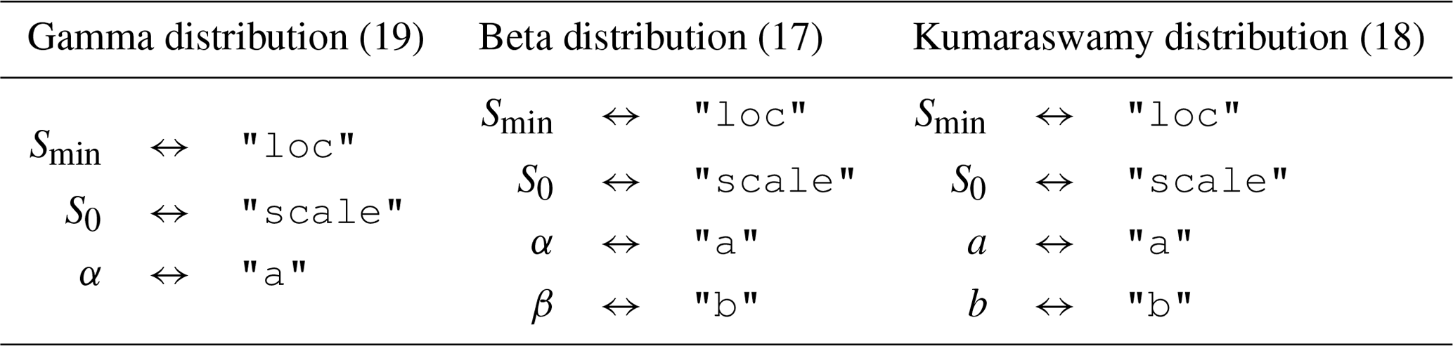
Table 1 The relationship between the parameters in Eqs. (17), (18), and (19) and the keys used to specify the value of these parameters in the SAS function specification.

Each of the keys naming a bulk flux in "sas_specs" is associated with a dictionary specifying the SAS functions for that flux. That dictionary can also include multiple SAS functions, which are combined together using time-varying weights. In the example above, mesas.py would expect to find columns in the time series dataset titled "Q SAS function 1" and "Q SAS function 2" containing weights to multiply each SAS function. These weights should add up to 1, although this is not checked. If the dictionary associated with each flux contains only one key:value pair, it is not necessary to provide a weights column in the time series dataset.

Presently, each SAS function can be specified in three different ways:

• as a gamma, beta, or Kumaraswamy distribution;

• using any distribution from scipy.stats;

• as a piecewise linear CDF.

The gamma, beta, or Kumaraswamy distributions are coded into the core computational code, whereas the scipy.stats distributions are approximated as piecewise linear CDFs. In either case, the distribution is selected based on the value associated with "func". In the example above, gamma and beta distributions are combined to produce the SAS function for outflow "Q".

The distribution parameters are given by the dictionary associated with the key "args". The expected content of this varies between distributions (see Table 1). Any parameter value can be specified as a fixed number or can be allowed to vary in time. Time-varying parameters are given as a string identical to a column in the time series dataset where the time-varying values are provided. In the example "sas_specs" above, the scale parameter of the gamma distribution used in "Q SAS function 1" is set to "S_scale". This tells mesas.py to use the time series of values found in that column of the input dataset for the scale parameter.

To use a distribution from scipy.stats the key:value pair "use":"scipy.stats" should be included. An optional parameter "nsegments" sets the number of segments used to approximate the distribution. Note that this approach is included for convenience but is not recommended when the tails of the SAS distribution are important for the problem being considered, as they may not be well captured by the piecewise linear CDF.

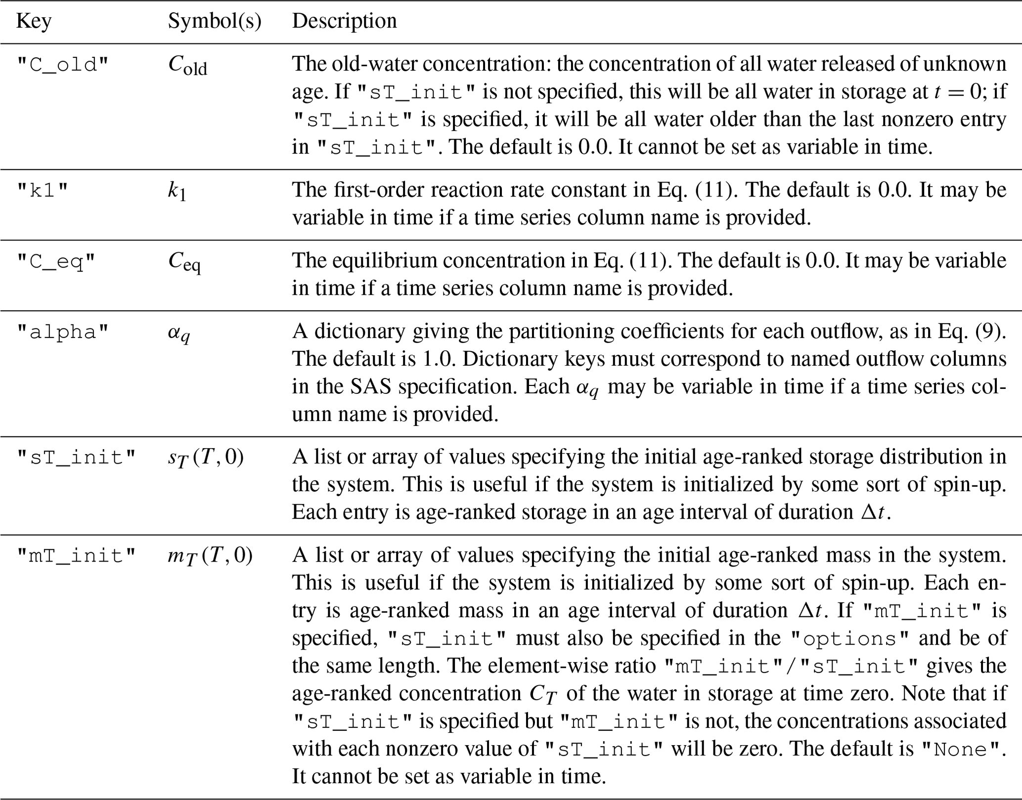
Table 2 Description of the keys that may optionally be associated with each solute in the "solute_parameters" section of the configuration file.

Alternatively, the SAS function can be specified as a piecewise linear CDF. In the example above, this option is used to specify a uniform SAS function for ET using a single linear segment. The cumulative age-ranked storage values "ST" and corresponding cumulative probabilities "P" (varying from zero to one) must be provided as lists of increasing values. Any of the values in these lists may be allowed to vary in time by instead providing a string corresponding to the heading of a column in the input time series dataset – see, for example, "S_ET" in the "ET SAS function" above.

3.2.2 Solute parameters

Solute properties are given in a dictionary associated with the top-level key "solute_parameters". The keys in this dictionary should correspond to columns in the time series dataset giving inflow concentrations. Each key should be associated with a dictionary giving additional parameters. If defaults are to be used, the associated dictionary may be empty and is then simply given as {}. An example is given below.

    "solute_parameters":{

        "Cl mg/l":{
            "C_old": 7.11,
            "alpha": {"Q": 1.0, "ET": 0.0}
        }
    },

In this case, mesas.py will look for a time series of solute inflows in column "Cl mg/l" and produce predictions of the outflow concentrations associated with this input. Two additional parameters are specified: "C_old" gives the old-water concentration (C_old) and "alpha" corresponds to the α_q partitioning parameter in Eq. (9). In the given example, no chloride can leave the system through ET, as the corresponding value of α is zero. See Table 2 for more information.

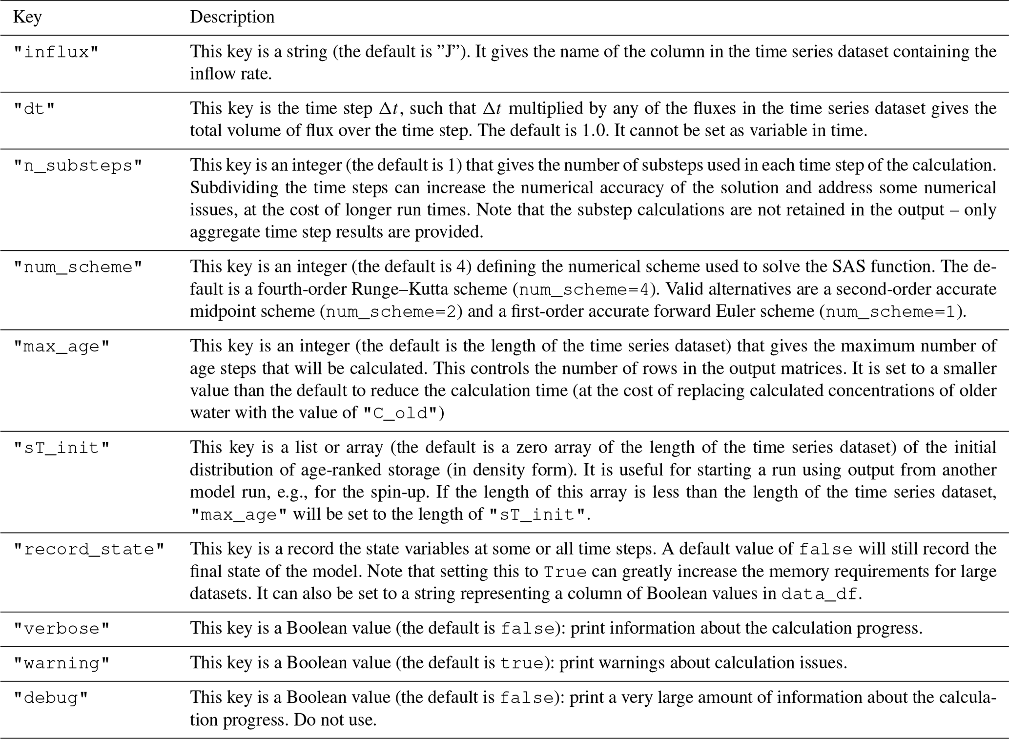
Table 3 Description of the keys that may optionally be in the "options" entry in the configuration file.

3.2.3 Options

Additional options can also be set in the "options" dictionary of the parameter inputs. The available options are described in Table 3.

3.2.4 Time series

The time series input can be provided as a .csv file or as a Python pandas data frame. The order of the columns is not important, but the column names should be consistent with references to time series data in the SAS function specification, solute parameters, and options.

For example, to be consistent with the specifications given in the example in Sect. 3.2.1 and 3.2.2, the input data frame would have the following columns:

• "Q" and "ET", which refer to the outflow rates (e.g., discharge and evapotranspiration, respectively) at each time step. These are assumed to be average rates over the time step (rather than instantaneous rates at the start or end).

• "J", which gives the average inflow rate over each time step.

• "Cl mg/l", which gives the inflow concentration at each time step.

• "Q SAS function 1" and "Q SAS function 2", which are weights associated with the two component SAS functions that will be combined to give the SAS function for "Q". Note that a column for "ET SAS function" is not required because there is only one component.

• "S_ET" and "S_scale", which are time-varying parameters of the SAS functions.

After running, the output time series would include the following new columns:

• "Cl mg/l --> Q",

• "Cl mg/l --> ET".

These time series represent the concentration of the solute in those outflow fluxes. The values of "Cl mg/l --> ET" would all be zero, as the partitioning coefficient "alpha" associated with that solute and outflow was set to zero.

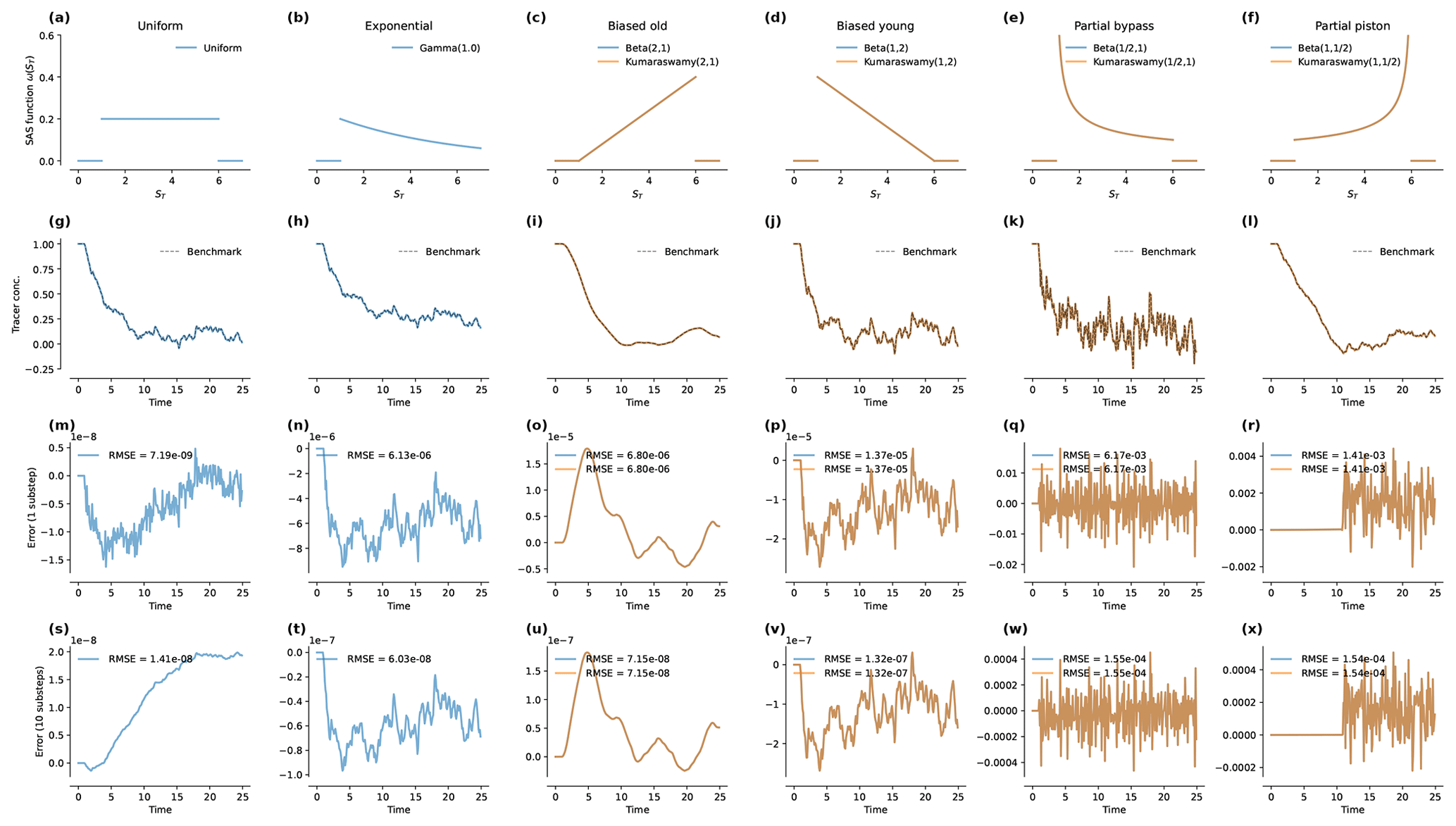
Figure 1 Results of the benchmark runs under steady flow. Panels (a) to (f) present the SAS functions used in each case. In each case, "loc"=1 and "scale"=5. The steady flow rate was Q=1 and the time step was Δt=0.1. Panels (g) to (l) show the predictions produced by mesas.py and the analytical benchmark solutions (dashed black lines). The inflow concentrations were Gaussian random variables with a mean of 1 and a standard deviation of 1. The initial concentration in storage was 1. Panels (m) to (r) give the absolute error relative to the benchmark with "n_substeps"=1. Panels (s) to (x) give the error with "n_substeps"=10. Note that the annotation “1e-6” on an axis indicates that the axis values are multiples of 10⁻⁶.

3.3 Running the model and querying results

The model is set up and run by instantiating a model object provided with all the needed input data and then calling its run method.

from mesas.sas.model import Model
my_model = Model(data_df='/path/to/data.csv',
 config='/path/to/config.json')
my_model.run()

The time series inputs and outputs will then be available in a data frame accessible as an attribute of the model object. For example, this would allow the user to plot the input and output concentrations.

import matplotlib.pyplot as plt

# Extract the timeseries
C_in = my_model.data_df['Cl mg/l']
C_out = my_model.data_df['Cl mg/l --> Q']
t = my_model.data_df.index

# Make the plots
plt.plot(t, C_in, label = "Cl in precip")
plt.plot(t, C_out, label = "Cl in discharge")

# Finishing touches
plt.legend(frameon=False)
plt.xlabel('time')
plt.ylabel('Cl [mg/l]')

Users can access further results by employing accessor functions. These can return the values for a particular time step, age step, or input time. The latter is useful for examining how water that entered at a particular time evolves in time. If none of these are given, the entire array is returned. Both density (sT, pQ, mT, mQ, and mR) and cumulative (ST, PQ, MT, MQ, and MR) forms are available.

# Make an array of ages to plot against
T = my_model.options['dt'] *
  np.arange(my_model.options['max_age'])

# Extract and plot the TTD at a particular
  timestep
pQ = my_model.get_pQ(timestep=100, flux='Q')
plt.figure()
plt.step(T, pQ, where='post')

# Extract and plot the volume of water
 in storage with an age less than 90
ST = my_model.get_ST(agestep=90)
plt.figure()
plt.step(T+1, ST, where='pre')

# Extract and plot the concentration
 of water in storage as it evolves due
  to evapoconcentration
sT = my_model.get_sT(inputtime=328)
mT = my_model.get_mT(inputtime=328,
  sol='Cl mg/l')
CT = mT/sT
plt.step(t, CT, where='post')

More information on these functions is available in the documentation (see the “Code and data availability” section of this paper).

4 Code validation and comparison

To validate the numerical implementation, mesas.py was tested against several analytical benchmark solutions. Six of these are analytical solutions for different SAS functions under steady-flow conditions. Additional benchmark solutions for unsteady flow are identical to those presented for tran-SAS in Benettin and Bertuzzo (2018) and can, therefore, be used for comparison.

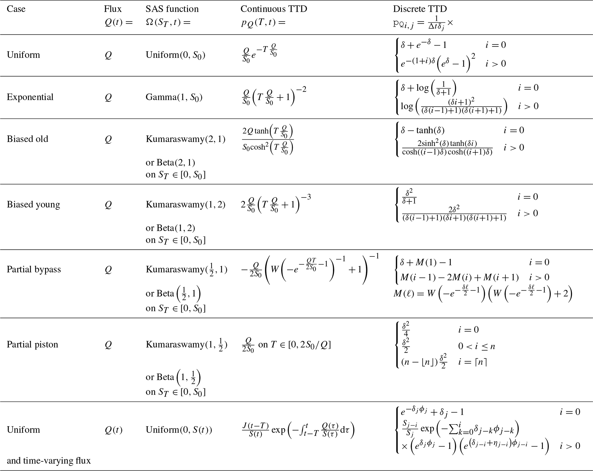
Table 4 Analytic solutions for the continuous and discrete TTD for a number of benchmark SAS functions with uniform, gamma, and beta distributions. The discrete form is obtained by averaging the value of p_Q over each age step and time step. In the time-variable cases, it is assumed that fluxes are constant over each time step, so $S_{j+\mathrm{1}}=S_j+\mathrm{\Delta }t(J_j-Q_j)$. For notational convenience, we have defined ${\mathit{\delta }}_j=\mathrm{\Delta }T{Q}_j/S_j$; κ=kΔt; ${\mathit{\eta }}_j=S_{j+\mathrm{1}}/S_j-\mathrm{1}$; $n=\frac{\mathrm{2}}{\mathit{\delta }}-\frac{\mathrm{1}}{\mathrm{2}}$; and ${\mathit{\varphi }}_j=\log ({\mathit{\eta }}_j+\mathrm{1})/{\mathit{\eta }}_j$ if η_j≠0 or ϕ_j=1 otherwise.

4.1 Validation against benchmarks: steady flow

4.1.1 Approach

For certain SAS functions, it is possible to find a closed-form expression for the corresponding TTD under steady flow. For the six cases considered here, the details of the derivations are given in Appendix A and the mathematical results are listed in Table 4. Several of these have been found previously (Botter, 2012; Harman, 2015; Berghuijs and Kirchner, 2017), although others are new.

The six cases (also shown in the top row of Fig. 1) are a uniform distribution; an exponential distribution; a “biased old” distribution and a “biased young” distribution, which encode a bias for older or younger storage, respectively, that varies linearly with age rank in storage; and a “partial piston” distribution and a “partial bypass” distribution, both of which encode a strong preference for the oldest and youngest storage, respectively. The latter four scenarios are special cases of both beta and Kumaraswamy distributions.

To assess the validity of our implementation of the numerical solution against these closed-form expressions, we can either (a) use very fine time steps, and thus more closely approximate the continuous result, or (b) find an analytical form of the discrete solution. The latter is preferable, as we can compare the numerical and analytical results directly, rather than asymptotically at the limit of small time steps. We have, therefore, taken the additional step of obtaining discrete versions of each expression (rightmost column of Table 4), which (when convolved with a synthetic time series of input concentrations) yield the average output concentration over each time step. These exact values can be compared directly to the numerical results, which are also intended to represent the average value over each time step.

In each scenario, the flow rate was set to $J\left(t\right)=Q\left(t\right)=\mathrm{1}$ and the time step to Δt=0.1. The value of the scale parameter was set to S₀=5, and an offset of S_min=1 was used. Consequently, outflow concentrations are delayed relative to inflows by five time steps. Inflow concentrations were synthetically generated as independent, identically distributed random values (white noise) that were normally distributed with a mean of 0.0 and a standard deviation of 1.0. Initial concentration in storage (C_old) was set to 1.0. The n_substeps parameter was initially set to 1 and then increased to 10 to examine how a greater number of numerical substeps improved the solution accuracy.

4.1.2 Results

Figure 1g–l plots the tracer concentration predicted by mesas.py (blue and orange lines, as labeled in the first row) and analytical benchmark solutions (dashed black line). The random inputs are smoothed most by the biased old case, and they retain much of the input variability in the partial bypass case. The last two rows of Fig. 1 present the percent errors relative to the benchmark when one (Fig. 1m–r) or 10 (Fig. 1s–x) numerical steps are taken each time step.

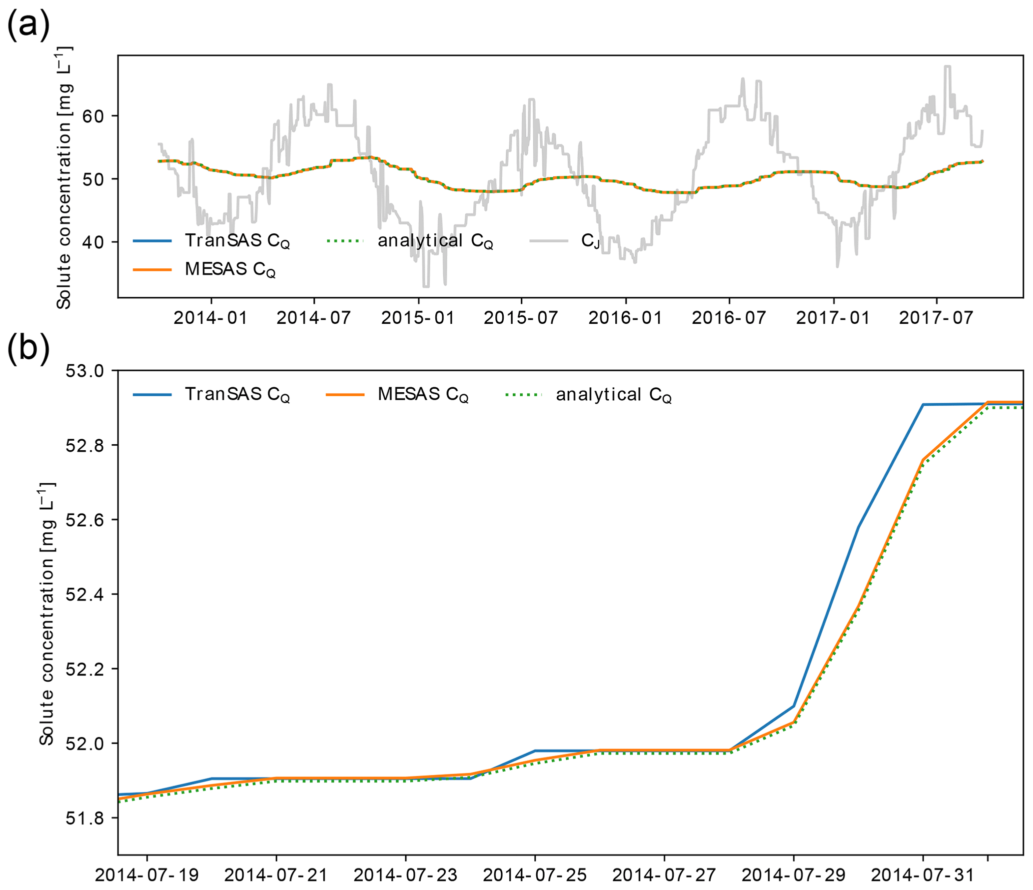
Figure 2 Comparison of mesas.py and tran-SAS for the case with uniform sampling and S₀=1000 mm. Panel (a) shows C_Q estimations from mesas.py (solid orange line) and tran-SAS (solid blue line) compared to the analytical solution (dashed green line); the solid gray line represents the input concentration from precipitation (C_J). Panel (b) presents a section of panel (a) in more detail, showing the errors resulting from the numerical scheme.

When n_substeps=1, the root-mean-square errors (RMSEs) for the uniform case were the smallest (at 10⁻⁹), whereas they were largest for the partial bypass and partial piston cases (whose errors are closer to 10⁻³). For the other three cases, the errors were around 10⁻⁶. When the number of substeps was increased to 10, the errors for those three cases (exponential, biased old, and biased young) decreased by a factor of 100. For the partial piston and partial bypass cases, the reduction was smaller (a factor of 9 and 40, respectively). For the uniform case, the error actually increased slightly, apparently due to a persistent (very small) bias associated with the initial concentration. When C_old was instead set to zero, the errors decrease by a factor of 2 when the substeps were increased.

In the partial piston case, errors are initially very low but suddenly become much larger later in the simulation. This occurs when the age-ranked storage of the oldest water in storage (that which entered in the first time step) reaches the “spike” on the right-hand end of the distribution. That is, using the definitions in Table 4, when $S_T(t,t)\approx S_{\mathrm{0}}$. The high curvature of Ω_Q at that point most stresses the ability of the numerical solution to accurately determine p_Q.

4.2 Validation against benchmarks: unsteady flow

4.2.1 Approach

The power of the SAS approach comes from its ability to handle time-variable inflows and outflows. The bottom row of Table 4 gives the analytical solution for a case in which the SAS function is uniform but the flow rate is variable in time. The general analytical solution was presented in Botter (2012), but the discrete form given here is novel. The discrete form is derived from the general case by assuming that inflows and outflow are constant over a time step, so that the storage varies linearly. Further, the solution given is not the instantaneous PDF p_Q but rather p_Q averaged over an age step/time step along a characteristic curve. Therefore, it gives a precise estimate of the expected value of the fraction of discharge over each time step drawn from inputs in previous time steps.

This benchmark was used to validate the mesas.py code for the same dataset that Benettin and Bertuzzo (2018) used to validate the performance of tran-SAS. The dataset was downloaded from the repository cited in Benettin and Bertuzzo (2018) and includes 8 years of 12 h precipitation, discharge, and evapotranspiration data. Benettin and Bertuzzo (2018) generated input concentrations by adding noise to a seasonal sinusoidal signal. The evapotranspiration was assumed to be drawn uniformly from the total storage in all simulations. Total storage at the end of each time step is calculated from the water balance assuming an initial storage S_init. The S₀ parameter used in mesas.py was calculated by averaging the total storage at the start and end of each time step.

4.2.2 Results

Figure 2 showcases the effect of activating some of the features of mesas.py: the ability to account for first-order reactions (for the case where the reaction rate is $\mathrm{3}\times {\mathrm{10}}^{-\mathrm{4}}$ h⁻¹) and fractionation (for a case in which α_ET=0.8, so that evapotranspiration enriches the tracer concentration in storage).

Figure 3 shows the input solute concentration as well as the output concentration predictions of mesas.py and tran-SAS for a case in which the discharge SAS function is uniform and S_init=1000 mm. Errors resulting from the numerical scheme are reduced in mesas.py relative to tran-SAS.

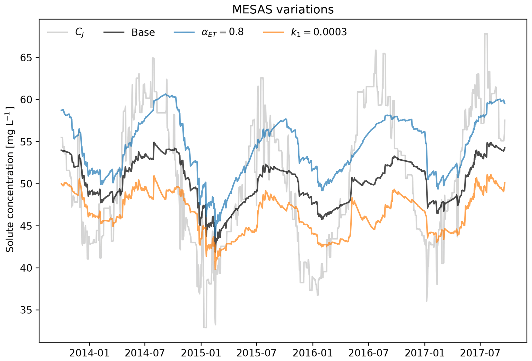
Figure 3 Variations of mesas.py applied to the time series and SAS model from Benettin and Bertuzzo (2018). The gray line shows the input concentration C_J from precipitation; the black line presents the base case, using the same setting as the tran-SAS model in Benettin and Bertuzzo (2018); the blue line denotes α_ET=0.8; and the orange line denotes a first-order reaction rate k₁=0.0003 d⁻¹.

Figure 4 Comparison of mesas.py with tran-SAS for a benchmark problem presented by Benettin and Bertuzzo (2018). Panel (a) shows the normalized RMSE of outflow concentration estimates from mesas.py (orange) and tran-SAS (blue) relative to the time-step-averaged analytical solution with S_init=1000 and k=1. Panel (b) presents the absolute concentration error CDF for mesas.py and tran-SAS. Panels (c) and (d) are the same as panels (a) and (b) but show errors in the mass flux, rather than the concentration. Panel (e) displays the effect of varying $k\in [\mathrm{0.2},\mathrm{0.3},\mathrm{0.5},\mathrm{1},\mathrm{1.2},\mathrm{1.5},\mathrm{2},\mathrm{3}]$ with S_init=1000 on the difference between each code's predictions and a run of mesas.py with 10 substeps as a high-accuracy estimate. Panel (f) shows the effect of varying $S_{\mathrm{init}}\in [\mathrm{300},\mathrm{500},\mathrm{1000},\mathrm{2000}]$ with k=1 on the concentration estimates of tran-SAS and mesas.py relative to the analytical solution.

Closer inspection of the residuals between the model concentration predictions and the analytical benchmarks reveals differences between the performance of tran-SAS and mesas.py. Figure 4a and b show the time series and distribution of errors for tran-SAS and mesas.py for a case in which S_init=1000 mm. Although the overall distribution of absolute error magnitudes is similar, tran-SAS produces relatively large errors about 15 % of the time. Overall, the RMSE of mesas.py is 0.3 % (of the output standard deviation), whereas the RMSE for tran-SAS is 1.5 %.

These differences become larger when we consider the error in the solute mass flux, as shown in Fig. 4c and d. The RMSE of mass flux in mesas.py is 0.016 %, whereas it is about 15 times larger for tran-SAS (0.21 %).

The differences can be almost entirely attributed to the fact that tran-SAS provides estimates of the instantaneous transit time distribution at the end of each time step, whereas mesas.py estimates time-step-averaged values. It is also possible to obtain the TTDs for the end of the time step from mesas.py output and use them to estimate outflow concentrations. Those estimates have errors (shown in green in Fig. 4d) very similar to those of tran-SAS, as we would expect.

mesas.py performs better than tran-SAS for other configurations of the problem, although the size of the difference changes. The normalized RMSEs of each implementation are shown in Fig. 4f for four different values of initial storage. The results show that the normalized RMSE is larger for both codes when storage is small; however, mesas.py has a lower RMSE than tran-SAS in all cases.

We can also compare the performance of these models for a case in which the discharge SAS function is not uniform. Again, following Benettin and Bertuzzo (2018), we consider the case in which ${\mathrm{\Omega }}_Q(S_T,t)={\left[\frac{S_T(T,t)}{S\left(t\right)}\right]}^k$. This is equivalent to a Kumaraswamy distribution with S_min=0, S₀=S(t), a=k, and b=1. The required parameter JSON file is given below.

    "sas_specs":{

        "Q":{
            "Q SAS function":{
                "func": "kumaraswamy",
                "args": {
                    "loc": 0.0,
                    "scale": "S",
                    "a": "k",
                    "b": 1.0
                }
            }
        },

        "ET":{
            "ET SAS function":{
                "ST": [0.0, "S"],
                "P":  [0.0, 1.0]
            }
        }
    },

    "solute_parameters":{
        "C":{
            "C_old": 50,
        }
    },

    "options":{
        "influx": "J"
        "n_substeps": 1
    },

The time series dataset includes columns "Q", "J", "ET", "S", "k", and input concentrations "C".

As analytical solutions are unavailable for this more general case, the results obtained from tran-SAS and mesas.py were compared against a higher-accuracy mesas.py solution (obtained by setting "n_substeps" to 10). The RMSEs for a range of values of k are shown in Fig. 4c. The mesas.py RMSE was consistently lower than that of tran-SAS. The RMSE for the mesas.py forward Euler is less than that of tran-SAS because it does not include the modification introduced by Benettin and Bertuzzo (2018) to improve the accuracy of the first age step.

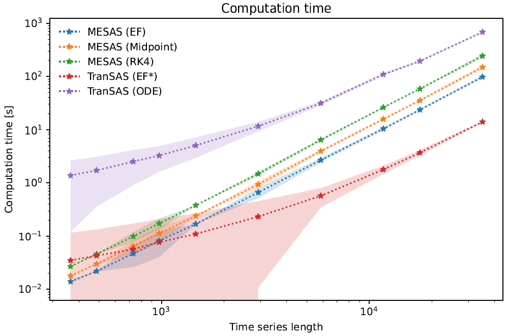
Figure 5 Comparison of the computational time and time series length for three mesas.py and two tran-SAS numerical computation settings. The plot shows the mean computational time and 95 % confidence interval for each case, represented by a line and corresponding colored region, respectively. The mesas.py cases include the EF (forward Euler), midpoint (midpoint method), and RK4 (fourth-order Runge–Kutta) methods, whereas the tran-SAS cases include the EF* (modified forward Euler) and ODE (MATLAB ODE solver) methods.

4.3 Performance

Computation time was compared by running all models for a benchmark configuration (with various lengths of time series) on a single-core Intel Xeon Gold Cascade Lake 6248R CPU with 192 GB DDR4 2933 MHz RAM. The benchmark configuration is the uniform sampling discharge SAS function case described above. Each configuration was run 100 times to establish confidence bounds on the run time.

As the results in Fig. 5 show, mesas.py and tran-SAS had comparable performance for time series less than 1000 time steps, but tran-SAS was generally computationally faster than mesas.py for longer time series. mesas.py was always faster than tran-SAS with the MATLAB ODE solver enabled. Using the midpoint and forward Euler numerical schemes in mesas.py resulted in a modest increase in performance (at the cost of numerical accuracy, as shown above).

5 Conclusions

SAS transport theory provides a very general framework for modeling material transport through control volumes (Benettin et al., 2022). At its core, it is based on a statement of conservation of mass of bulk material of different ages. This must be augmented with an SAS function that captures how outflow preferentially removes bulk material from storage according to the rank of its age. The mesas.py code presented here implements this theory, allows SAS functions to be expressed in a very flexible way, and solves the underlying equations with high accuracy with regard to mass balance.

The code is also intended to be user-friendly. A number of resources are available, including a free online course via HydroLearn. The course, entitled “JHU 570.412 Tracers and transit times in time-variable hydrologic systems: A gentle introduction to the StorAge Selection (SAS) approach” can be found at https://edx.hydrolearn.org/courses/course-v1:JHU+570.412+Sp2020/course/ (last access: 8 November 2023) (free registration required). This course includes three sections of introductory SAS function theory accompanied by a mesas.py walk-through.

Further work is needed to augment the code with additional useful tools. Three sets of tools are particularly important. First, tools for generating ensembles of input concentration data. In hydrology, observations of input concentrations are often bulk samples that represent amount-weighted averages over multiple time steps. These must be disaggregated to the resolution at which we want to run the model. Second, tools for parameterizing SAS functions and fitting them to data, preferably in a way that can adapt to any specification of the SAS function. Third, tools for assessing uncertainty in both the disaggregated inputs, the SAS function shape, and the model predictions.

Appendix A: Analytical benchmarks

A1 Steady-state solutions

At steady state with one outflow and J=Q, Eq. (2) can be written as follows:

$$\begin{array}{}\text{(A1)}& {\displaystyle \frac{\mathrm{d}{s}_T}{\mathrm{d}T}}=-Q{p}_Q\left(T\right),\text{(A2)}& {\displaystyle }{s}_T\left(\mathrm{0}\right)=Q.\end{array}$$

This is a separable differential equation, which we can integrate twice to give the following:

$$\begin{array}{}\text{(A3)}& S_T\left(T\right)=Q\left(T-\underset{\mathrm{0}}{\overset{T}{\int }}{P}_Q\left(\mathit{\tau }\right)\mathrm{d}\mathit{\tau }\right).\end{array}$$

This gives the steady-state cumulative age-ranked storage in terms of the cumulative transit time distribution P_Q.

Alternatively, we can use the fact that p_Q=ω_Qs_T and $s_T=\mathrm{d}{S}_T/\mathrm{d}T$ to write the conservation law as follows:

$$\begin{array}{}\text{(A4)}& {\displaystyle \frac{\mathrm{d}{S}_T}{\mathrm{d}T}}=Q-Q{\mathrm{\Omega }}_Q\left(S_T\right(T\left)\right),\text{(A5)}& {\displaystyle }{S}_T\left(\mathrm{0}\right)=\mathrm{0}.\end{array}$$

This can likewise be integrated to obtain the age of water at a given location in age-ranked storage in terms of the SAS function:

$$\begin{array}{}\text{(A6)}& T={\displaystyle \frac{\mathrm{1}}{Q}}\underset{\mathrm{0}}{\overset{S_T\left(T\right)}{\int }}{\displaystyle \frac{\mathrm{1}}{\mathrm{1}-{\mathrm{\Omega }}_Q\left(\mathit{\sigma }\right)}}\mathrm{d}\mathit{\sigma }.\end{array}$$

Using these equations, we can (in principle) find the steady-state transit time distributions if we know the SAS function, and vice versa. In many cases, a closed-form solution is not possible.

For example, for a uniform distribution U(0,S₀), the SAS function is given by ${\mathrm{\Omega }}_Q\left(S_T\right)=S_T/S_{\mathrm{0}}$ for $S_T\in [\mathrm{0},S_{\mathrm{0}}]$. Substituting this into Eq. (A6) gives $QT=-S_{\mathrm{0}}\log \left(\mathrm{1}-S_T/S_{\mathrm{0}}\right)$, and rearranging gives $S_T\left(T\right)=S_{\mathrm{0}}\left(\mathrm{1}-e^{\frac{Q}{S_{\mathrm{0}}}T}\right)$. This is the cumulative age-ranked storage when Ω_Q is a uniform distribution and the flow is steady. Substituting this into the definition of the uniform Ω_Q yields the cumulative transit time distribution (as $P_Q(T,t)={\mathrm{\Omega }}_Q(S_T,t)$ by definition). Consequently, we can say that

$$\begin{array}{}\text{(A7)}& {\mathrm{\Omega }}_Q\left(S_T\right)=U(\mathrm{0},S_{\mathrm{0}})\iff P_Q\left(T\right)=\mathrm{1}-e^{-\frac{Q}{S_{\mathrm{0}}}T}\end{array}$$

at steady state. That is, a uniform SAS function is equivalent to an exponential TTD.

A similar set of steps can be used to show that an exponential SAS function (which is a special case of a gamma distribution with shape parameter α=1) is equivalent to a TTD following a Lomax distribution with exponent 1:

$$\begin{array}{}\text{(A8)}& {\mathrm{\Omega }}_Q\left(S_T\right)=\mathrm{\Gamma }(\mathrm{1},S_{\mathrm{0}})\iff P_Q\left(T\right)=\mathrm{1}-{\left(\mathrm{1}+QT/S_{\mathrm{0}}\right)}^{-\mathrm{1}}.\end{array}$$

We were not able to obtain a solution for the general case of a gamma distribution. Similarly, solutions for the TTD when the SAS function is given by a beta distribution B(α,β) over $\mathrm{0}\le S_T/S_{\mathrm{0}}\le \mathrm{1}$ could only be found for particular values of (α,β). For example, with α=1 and β=2, we have the biased young case:

$$\begin{array}{}\text{(A9)}& {\mathrm{\Omega }}_Q\left(S_T\right)=B(\mathrm{1},\mathrm{2})\iff P_Q\left(T\right)=\mathrm{1}-{\left(\mathrm{1}+TQ/S_{\mathrm{0}}\right)}^{-\mathrm{2}},\end{array}$$

which is a Lomax distribution with exponent 2. Similarly the biased old, partial bypass, and partial piston cases are as follows:

$$\begin{array}{}\text{(A10)}& {\displaystyle }{\mathrm{\Omega }}_Q\left(S_T\right)=B(\mathrm{2},\mathrm{1})\iff P_Q\left(T\right)={\tanh }^{\mathrm{2}}\left(TQ/S_{\mathrm{0}}\right),\text{(A11)}& {\displaystyle }\begin{array}{rl}{\mathrm{\Omega }}_Q\left(S_T\right)& =B\left(\frac{\mathrm{1}}{\mathrm{2}},\mathrm{1}\right)\iff P_Q\left(T\right)\\ & =W\left(-e^{-\frac{QT}{\mathrm{2}{S}_{\mathrm{0}}}-\mathrm{1}}\right)+\mathrm{1},\end{array}\text{(A12)}& {\displaystyle }\begin{array}{rl}{\mathrm{\Omega }}_Q\left(S_T\right)& =B(\mathrm{1},\mathit{\beta })\iff P_Q\left(T\right)=\mathrm{1}-\left(\right(\mathit{\beta }-\mathrm{1})\\ & QT/S_{\mathrm{0}}+\mathrm{1}{)}^{\frac{\mathit{\beta }}{\mathrm{1}-\mathit{\beta }}}.\end{array}\end{array}$$

Here, W(⋅) is the Lambert W function.

A2 Accounting for discretization effects

To obtain a discrete form of the analytical solution, we can make two assumptions. First, that the time series of inflow concentrations and of water inflows and outflows are in fact constant within a time step Δt, so

$$\begin{array}{}\text{(A13)}& {\displaystyle }{{\mathtt{C}}_{\mathtt{J}}}_j=C_J\left(t\right)\text{ for }j\le t/\mathrm{\Delta }t<j+\mathrm{1},\text{(A14)}& {\displaystyle }{\mathtt{J}}_j=J\left(t\right)\text{ for }j\le t/\mathrm{\Delta }t<j+\mathrm{1},\text{(A15)}& {\displaystyle }{\mathtt{Q}}_j=Q\left(t\right)\text{ for }j\le t/\mathrm{\Delta }t<j+\mathrm{1}.\end{array}$$

Here, ${{\mathtt{C}}_{\mathtt{J}}}_j$ and ${{\mathtt{C}}_{\mathtt{Q}}}_j$ are the discrete forms of C_J(t) and C_Q(t).

Second, we assume that the numerical estimates of the outflow concentration time series should reflect the average value of the analytical solution over each time step. That is,

$$\begin{array}{}\text{(A17)}& {{\mathtt{C}}_{\mathtt{Q}}}_j={\displaystyle \frac{\mathrm{1}}{\mathrm{\Delta }t}}\underset{\mathrm{0}}{\overset{\mathrm{\Delta }t}{\int }}{C}_Q(j\mathrm{\Delta }t+\mathit{\nu })\mathrm{d}\mathit{\nu }.\end{array}$$

In the continuous form, C_Q is obtained by the convolution of p_Q with C_J, as shown in Eq. (1). If we assume that the input concentrations are constant over each time step, Eq. (1) can be expressed as the sum of integrals over each time step interval $j\mathrm{\Delta }t\le t<(j+\mathrm{1})\mathrm{\Delta }t$ with the subsequent addition the old-water contribution:

$$\begin{array}{}\text{(A18)}& \begin{array}{rl}{C}_Q\left(t\right)& =\underset{\mathrm{0}}{\overset{t}{\int }}{C}_J(t-T)p_Q(T,t)\mathrm{d}T+C_{\mathrm{old}}{P}_Q(t,t)\\ & =\left(\sum _{i=\mathrm{0}}^{j-\mathrm{1}}\underset{t-(j-i))\mathrm{\Delta }t}{\overset{t-(j-i-\mathrm{1})\mathrm{\Delta }t}{\int }}{C}_J(t-T)p_Q(T,t)\mathrm{d}T\right)\\ & +\underset{\mathrm{0}}{\overset{t-j\mathrm{\Delta }t}{\int }}{C}_J(t-T)p_Q(T,t)\mathrm{d}T+C_{\mathrm{old}}{P}_Q(t,t)\\ & =\left(\sum _{i=\mathrm{0}}^{j-\mathrm{1}}{{\mathtt{C}}_{\mathtt{J}}}_{j-i-\mathrm{1}}\underset{t-(j-i))\mathrm{\Delta }t}{\overset{t-(j-i-\mathrm{1})\mathrm{\Delta }t}{\int }}{p}_Q(T,t)\mathrm{d}T\right)\\ & +{{\mathtt{C}}_{\mathtt{J}}}_j\underset{\mathrm{0}}{\overset{t-j\mathrm{\Delta }t}{\int }}{p}_Q(T,t)\mathrm{d}T+C_{\mathrm{old}}{P}_Q(t,t)\\ & =\left(\sum _{i=\mathrm{0}}^{j-\mathrm{1}}{{\mathtt{C}}_{\mathtt{J}}}_{j-i-\mathrm{1}}\left(P_Q(t-(j-i-\mathrm{1})\mathrm{\Delta }t,t)\right.\right.\\ & \left.\left.-P_Q(t-(j-i)\mathrm{\Delta }t,t)\right)\right)+{{\mathtt{C}}_{\mathtt{J}}}_j{P}_Q\\ & (t-j\mathrm{\Delta }t,t)+C_{\mathrm{old}}{P}_Q(t,t).\end{array}\end{array}$$

To obtain the discrete outflow concentrations, we must apply the time step averaging in Eq. (A17) to Eq. (A18), which yields the discrete convolution:

$$\begin{array}{}\text{(A19)}& {{\mathtt{C}}_{\mathtt{Q}}}_j=\sum _{i=\mathrm{0}}^j{{\mathtt{C}}_{\mathtt{J}}}_{j-i}{{\mathtt{p}}_{\mathtt{Q}}}_{i,j}\mathrm{\Delta }t+C_{\mathrm{old}}{{\mathtt{P}}_{\mathtt{Q}}}_{j,j}.\end{array}$$

Here, the time-step-averaged TTD ${{\mathtt{P}}_{\mathtt{Q}}}_{i,j}$ is given by

$$\begin{array}{}\text{(A20)}& {{\mathtt{P}}_{\mathtt{Q}}}_{i,j}={\displaystyle \frac{\mathrm{1}}{\mathrm{\Delta }t}}\underset{\mathrm{0}}{\overset{\mathrm{\Delta }t}{\int }}{P}_Q(i\mathrm{\Delta }t+\mathit{\nu },j\mathrm{\Delta }t+\mathit{\nu })\mathrm{d}\mathit{\nu }.\end{array}$$

${{\mathtt{p}}_{\mathtt{Q}}}_{i,j}$ is obtained via the discrete derivative

$$\begin{array}{}\text{(A21)}& {{\mathtt{p}}_{\mathtt{Q}}}_{i,j}=\left\{\begin{array}{ll}{\displaystyle \frac{{{\mathtt{P}}_{\mathtt{Q}}}_{i,j}}{\mathrm{\Delta }t}}& i=\mathrm{0}\\ \\ {\displaystyle \frac{{{\mathtt{P}}_{\mathtt{Q}}}_{i,j}-{{\mathtt{P}}_{\mathtt{Q}}}_{i-\mathrm{1},j}}{\mathrm{\Delta }t}}& i>\mathrm{0}.\end{array}\right.\end{array}$$

For the elementary case of steady flow and uniform sampling, this gives

$$\begin{array}{}\text{(A22)}& {{\mathtt{p}}_{\mathtt{Q}}}_{i,j}={\displaystyle \frac{\mathrm{1}}{\mathrm{\Delta }t\mathit{\delta }}}\times \left\{\begin{array}{ll}\mathit{\delta }+e^{-\mathit{\delta }}-\mathrm{1}& i=\mathrm{0}\\ e^{-(\mathrm{1}+i)\mathit{\delta }}{\left(e^{\mathit{\delta }}-\mathrm{1}\right)}^{\mathrm{2}}& i\ge \mathrm{1},\end{array}\right.\end{array}$$

where $\mathit{\delta }=\mathrm{\Delta }tQ/S_{\mathrm{0}}$. Other forms are given in Table 4. Note that δ must be less than 1 in the exponential and biased young cases.