Assessment of a tiling energy budget approach in a land surface model, ORCHIDEE-MICT (r8205)

The surface energy budget plays a critical role in terrestrial hydrological and biogeochemical cycles. Nevertheless, its highly spatial heterogeneity across different vegetation types is still missing in the ORCHIDEE-MICT (ORganizing Carbon and Hydrology in Dynamic EcosystEms–aMeliorated Interactions between Carbon and Temperature) land surface model. In this study, we describe the representation of a tiling energy budget in ORCHIDEE-MICT and assess its short-term and long-term impacts on energy, hydrology, and carbon processes. With the specific values of surface properties for each vegetation type, the new version presents warmer surface and soil temperatures (∼ 0.5 °C, +3 %), wetter soil moisture (∼ 10 kg m⁻², +2 %), and increased soil organic carbon storage (∼ 170 Pg C, +9 %) across the Northern Hemisphere. Despite reproducing the absolute values and spatial gradients of surface and soil temperatures from satellite and in situ observations, the considerable uncertainties in simulated soil organic carbon and hydrological processes prevent an obvious improvement in the temperature bias existing in the original ORCHIDEE-MICT model. However, the separation of sub-grid energy budgets in the new version improves permafrost simulation greatly by accounting for the presence of discontinuous permafrost types (∼ 3×10⁶ km²), which will facilitate various permafrost-related studies in the future.

1 Introduction

The surface energy balance is a fundamental component of the Earth system. The incoming solar energy is not only essential for life and plant photosynthesis but also drives the terrestrial hydrological cycle (i.e., evapotranspiration and the freeze–thaw cycle of soils in cold regions) and modulates the speed of biogeochemical reactions (i.e., the decomposition of organic matter). The energy balance depends on the landscape type through distinct vegetation and soil elements that reflect and emit shortwave and longwave electromagnetic radiation in different proportions. Understanding and simulating the complex interactions of energy, hydrology, and biogeochemical processes throughout the Earth system is crucial for tracking the consequences of historical human activities and predicting the future of our Earth's climate system.

Employing land surface models (LSMs) or Earth system models (ESMs) is one of the most common approaches to simulate the surface energy budget and investigate its interactions with hydrological, atmospheric, and biogeochemical processes. The typical spatial resolution of LSMs varies from 0.5° × 0.5° (∼ 50 km × 50 km at the Equator) to 2° × 2° (∼ 200 km × 200 km at the Equator). Significant surface heterogeneity would undoubtedly exist on such large scales. Taking surface temperature (T_surf) as an example, in reality, two adjacent landscapes could have significantly different T_surf values due to their distinct surface properties, including surface albedo, leaf area index, rooting depth, and vegetation height, at a scale not resolved by the models. For instance, the larger latent heat loss via evapotranspiration over deep-rooted tropical forests compared with nearby grassland and cropland shows a significant cooling effect, approximately 2.5 °C on a daily basis (Li et al., 2015). The higher albedo across snow-covered areas for short vegetation compared with nearby forest results in a reduction in the absorbed solar energy and a lower T_surf, with a magnitude depending on the timing and duration of snow cover (Zhang, 2005). To represent the heterogeneous surface energy balance, some LSMs/ESMs have introduced tiling energy budgets, such as the plant-functional-type-specific energy budgets in CLASSIC (Canadian Land Surface Scheme Including Biogeochemical Cycles; Melton and Arora, 2014); the separate energy budgets for snow, soil, and vegetation in ISBA (Soil–Biosphere–Atmosphere LSM; Boone et al., 2017); the partitioning of snow-covered and snow-free land units in CLM 5.0 (Community Land Model; Lawrence et al., 2019); and the sub-grid topographic effects on solar radiation flux in ELM (the Energy Exascale Earth System Model (E3SM) Land Model; Hao et al., 2021). Moreover, three land surface schemes (LSSs) have been adopted to represent the tiling energy budgets: mosaic (the use of specific surface properties for each land cover type), mixed (the grouping of certain land cover types with similar surface properties and the consequent use of a smaller number of distinct surface types), and composite (the use of the average properties of one grid cell) (Melton and Arora, 2014; Rumbold et al., 2023). Through a comparison of the mosaic and the composite LSSs, the CLASSIC model reported a less than 5 % difference in the primary energy fluxes but an up to 46 % difference in carbon fluxes and the carbon pool size at the site level (Li and Arora, 2012); the aforementioned model also found a 19 % higher terrestrial carbon sink for 1959–2005 in the mosaic simulation (Melton and Arora, 2014). Moreover, using the JULES (Joint UK Land Environment Simulator) model, Rumbold et al. (2023) found that the tiling soil scheme does have an impact on the water and energy budgets due to the way vegetation accesses soil moisture. Furthermore, Qin et al. (2023) reported that the tiling CLM model provides more accurate simulations of surface air temperature and precipitation than the single-land-cover version when coupled with the WRF (Weather Research and Forecasting) model, as validated against in situ observations. Despite uncertainties in model-specific structures and configurations, these findings highlight the importance of explicitly representing sub-grid surface heterogeneity in current LSMs.

Besides the necessity to represent surface heterogeneity, the incorporation of new landforms and processes also requires the tiling of energy budgets. For instance, Rooney and Jones (2010) identified the challenges involved in simulating soil temperature under lakes when introducing lakes into the single-soil-tile JULES model, as they have different thermal transfer characteristics due to the higher specific heat capacity of water than adjacent land tiles. When evaluating the impacts of sub-grid-scale disturbances, such as fires and harvest, Curasi et al. (2023) found that the impact of sub-grid heterogeneity is 1.5–4 times the impact of the disturbances themselves on the carbon cycle with the CLASSIC model. Moreover, it is necessary to provide the independent energy budgets, hydrology, and carbon cycles when incorporating a series of new processes for permafrost regions, such as discontinuous permafrost (Smith et al., 2022), melting of ground ice (Rumbold et al., 2023), thermokarst thawing, and lateral drainage (Nitzbon et al., 2020), in LSMs.

To enable the representation of surface heterogeneity and open the door to a series of new landforms and processes, we implement tiling energy budgets at the surface and subsurface for each plant functional type (PFT) in a state-of-the-art LSM, ORCHIDEE-MICT (ORganizing Carbon and Hydrology in Dynamic EcosystEms–aMeliorated Interactions between Carbon and Temperature), which calculates turbulent fluxes for sub-grid PFTs but solves for an average grid-level energy budget, resulting in a single surface temperature (Guimberteau et al., 2018). Some hydrological and biogeochemical processes in the model have been modified correspondingly to include PFT-specific thermal inputs. In Sect. 2, we provide a brief review of the current grid cell mean energy budget at the surface and subsurface, while Sect. 3 describes the modifications made to implement the tiling energy budgets in the model. To evaluate the impacts of separating the energy budget for each PFT on the energy, hydrology, soil thermodynamics, and carbon cycles, we conduct simulations using the original version of ORCHIDEE-MICT (referred to as MICT) and the new tiling energy budget version (referred to as MICT-teb), as described in Sect. 4. The results of these simulations are compared in Sect. 5. Section 6 focuses on the evaluation of energy processes in the new version as well as the improvements for permafrost simulations. Finally, we present conclusions in Sect. 7.

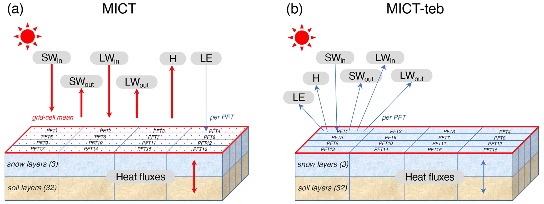
Figure 1 Schematic representation of energy budgets at the surface, snow layers, and soil layers in one grid cell of ORCHIDEE-MICT (MICT) (a) and the new tiling energy budget version (MICT-teb) (b). SW_in, SW_out, LW_in, LW_out, H, and LE represent incoming shortwave radiation, outward shortwave radiation, incoming longwave radiation, outward longwave radiation, sensible heat flux, and latent heat flux, respectively. PFT indicates the plant functional type. There are 3 layers for snow and 32 layers for soil for each PFT in the model. In MICT, SW_in, SW_out, LW_in, LW_out, H, and heat fluxes in the snow and soil layers are calculated as a grid cell mean, but LE is calculated for each PFT; in MICT-teb, all of the heat fluxes are calculated for each PFT. The red and blue arrows denote the grid cell mean and the PFT-specific calculations, respectively.

2 Overview of the current energy budget in ORCHIDEE-MICT

ORCHIDEE-MICT is a branch of the ORCHIDEE model (Krinner et al., 2005) that has been specifically developed to enhance the representation of hydrological and biogeochemical interactions in high-latitude regions (Guimberteau et al., 2018). In comparison with the trunk version 3976 from which it was developed, ORCHIDEE-MICT includes several key new processes: (1) the feedback effects of the soil organic carbon (SOC) concentration on soil thermal and soil water dynamics (Zhu et al., 2019); (2) soil carbon vertical discretization (Koven et al., 2009; Zhu et al., 2016); (3) vertical mixing of soil carbon due to cryoturbation (in cold soils) and bioturbation (Koven et al., 2009, 2013); (4) reformulation of soil hydric stress above the permafrost table (Zhu et al., 2015); and (5) the inclusion of northern peatlands as a specific PFT with peatland-specific hydrology, carbon decomposition, and accumulation (Qiu et al., 2018, 2019). These new processes have significantly improved the representation of plant productivity, the water cycle, soil carbon stocks, and the simulated permafrost distribution in high-latitude regions, but there is still room for improvement (Guimberteau et al., 2018). One important aspect that calls for attention is the need to include sub-grid representations of surface and subsurface energy budgets, especially at high latitudes where the snow cover and water equivalent differ between PFTs and where soil carbon differences across landscape elements/PFTs within the same grid cell result in a heterogeneous soil temperature and active layer thickness. For the moment, within the ORCHIDEE-MICT model, there are three major modules: carbon, water, and energy. The carbon cycle module operates for each PFT sub-grid, the water cycle operates for each soil tile (divided into bare soil, tree PFTs, grass and crop PFTs, and peatland PFT categories), and the energy module is solved only at the total grid cell level (Best et al., 2004). Figure 1 shows the schematic representation of the energy budgets from the surface to snow and soil layers in the original and new versions of ORCHIDEE-MICT, namely MICT and MICT-teb, respectively. The details of the energy budget in the model are outlined in the following.

2.1 Surface energy budgets

Similar to most LSMs, the surface energy budget equation is used in MICT to describe the balance of net absorbed radiation (R_net) by the energy transferred out of the ecosystem:

$$\begin{array}{}\text{(1)}& R_{\text{net}}=H+\mathit{\text{LE}}+G+\mathrm{\Delta }S,\end{array}$$

where H is the sensible heat flux (W m⁻²), LE is the latent heat flux (W m⁻²), G is the ground heat flux (W m⁻²), and ΔS is the energy stored in the ecosystem as chemical energy through photosynthesis and as the temperature change in the plant biomass (W m⁻²). Due to the ΔS only accounting for < 5 % of the total energy budget of the ecosystem in most areas (Georg et al., 2016), it is neglected in the model. R_net is the balance of the inputs and outputs of shortwave radiation (SW_in and SW_out) and longwave radiation (LW_in and LW_out):

$$\begin{array}{}\text{(2)}& \begin{array}{rl}{R}_{\text{net}}& =({\mathrm{SW}}_{\mathrm{in}}-{\mathrm{SW}}_{\mathrm{out}})+({\mathrm{LW}}_{\mathrm{in}}-{\mathrm{LW}}_{\mathrm{out}})\\ & =(\mathrm{1}-\mathit{\alpha })\times {\mathrm{SW}}_{\mathrm{in}}+\left({\mathrm{LW}}_{\mathrm{in}}-\mathit{\sigma }\times \mathit{\epsilon }\times (T_{\text{surf}}{)}^{\mathrm{4}}\right),\end{array}\end{array}$$

where α is the albedo, which determines the proportion of incoming SW absorbed by the ecosystem (unitless); σ is the Stefan–Boltzmann constant (5.6697 × 10⁻⁸ $\mathrm{W}{\mathrm{m}}^{-\mathrm{2}}{\mathrm{K}}^{-\mathrm{4}}$); ε is the emissivity (1, unitless); and T_surf is the surface temperature (K). In MICT, the grid cell α is calculated as the area-weighted average of the α values across all PFTs. The snow-covered areas and snow-free areas are distinguished in terms of the higher albedo of snow than canopy and bare soil (see Sect. 2.3 for details on the calculation of albedo for snow-covered regions). The albedo of bare soil in the current version is prescribed using static satellite observations (Lurton et al., 2020), with the background albedo extracted using the Joint Research Centre Two-stream Inversion Package (Pinty et al., 2011); thus, it is calculated without interannual variations and decoupled from simulated soil moisture (Fig. S1 in the Supplement). The albedo of vegetated PFTs is prescribed with constant values in the model (Table S1 in the Supplement). As MICT is not capable of calculating leaves' energy budgets separately from those of the soil and stem, there is no vertically layered temperature from the ground surface to the top of the canopy; thus, the T_surf is used to calculate all surface energy fluxes here. The two heat fluxes out of the surface, i.e., H and LE, are calculated following Eqs. (3) and (4), respectively:

$$\begin{array}{}\text{(3)}& {\displaystyle }& {\displaystyle }H=\mathit{\rho }\times v\times C_{\mathrm{d}}\times c_p\times (T_{\text{surf}}-T_{\text{air}}),\text{(4)}& {\displaystyle }& {\displaystyle }\mathit{LE}=L\times \mathit{\beta }\times \mathit{\rho }\times v\times C_{\mathrm{d}}\times (q_{\text{surf}}-q_{\text{air}}),\end{array}$$

where ρ is air density (kg m⁻³); v is the horizontal wind speed (m s⁻¹); C_d is the drag coefficient (unitless); c_p is the specific heat capacity of dry air (1004.675 $\mathrm{J}{\mathrm{kg}}^{-\mathrm{1}}{\mathrm{K}}^{-\mathrm{1}}$); T_air is the air temperature (K); L is the latent heat of evaporation or sublimation (2.5008 or 2.8345 × 10⁶ J kg⁻¹); β is the limiting factor of potential total evapotranspiration (PET) (unitless); and q_surf and q_air are the saturated moisture at the surface and in the air (kg kg⁻¹), respectively. Due to the differences in the canopy height and leaf area index (LAI), C_d should be different among different PFTs. To ensure compatibility with the grid cell calculation of the surface energy budget, the C_d of different PFTs is weighted by their area. The LE (or ET) serves as the link between the energy cycle and the hydrological and carbon cycle. It is PFT-specific via a PFT-specific β (see details in Ducharne, 2018) because the carbon cycle and hydrological processes separate different PFTs or different soil tiles. In MICT, the LE consists of E_flood (flood evaporation, not activated in the simulations of this study), E_subli (snow sublimation), E_soil (evaporation from bare soil), E_trans (transpiration), and E_inter (interception). Due to the distinct plant structures between different PFTs, the evaporation components associated with vegetation, i.e.,  E_trans and E_inter are PFT-specific, whereas the E_subli and E_soil are calculated as the grid cell average. For G, the energy exchange between the surface and ground (snow or soil depending on the snow cover fraction) is calculated following the classic Fourier law (Hourdin, 1992). Considering that the calculation of G is identical to heat conduction in soil layers, the detailed derivation is only shown in Sect. 2.2 to avoid redundancy. For the areas covered by snow, G also considers heat fluxes into the snowpack which are used to melt snow.

2.2 Soil energy budgets

Table S2 in the Supplement displays the vertical discretization of soil in the current version of MICT. There are 32 soil layers for soil heat conduction with a total depth of 38 m and 11 soil layers for soil hydrology with a total depth of 2 m. These soil layers are located below the three snow layers in the model when there is snow (Fig. 1a). As mentioned earlier, the heat conduction across soil layers, snow layers, and between the surface and ground is calculated using the classic one-dimensional Fourier law (Hourdin, 1992), with the latent flux of soil freezing taken into consideration (Gouttevin et al., 2012):

$$\begin{array}{}\text{(5)}& c{\displaystyle \frac{\partial T_{\text{soil}}}{\partial t}}={\displaystyle \frac{\partial }{\partial z}}\left(\mathit{\lambda }{\displaystyle \frac{\partial T_{\text{soil}}}{\partial z}}\right)+{\mathit{\rho }}_{\text{ice}}L{\displaystyle \frac{\partial {\mathit{\theta }}_{\text{ice}}}{\partial t}},\end{array}$$

where c is the volumetric soil heat capacity ($\mathrm{J}{\mathrm{K}}^{-\mathrm{1}}{\mathrm{m}}^{-\mathrm{3}}$), T_soil is the soil temperature (K), λ is the soil thermal conductivity ($\mathrm{J}{\mathrm{m}}^{-\mathrm{1}}{\mathrm{s}}^{-\mathrm{1}}{\mathrm{K}}^{-\mathrm{1}}$), ρ_ice is the ice density (920 kg m⁻³), L is the latent heat of fusion (0.3336 × 10⁶ J kg⁻¹), θ_ice is the volumetric ice content (m³ m⁻³), t is time (s), and z is the soil layer depth (m). The c is calculated as the area-weighted sum of the heat capacity of liquid soil moisture (4.18 × 10⁶ $\mathrm{J}{\mathrm{K}}^{-\mathrm{1}}{\mathrm{m}}^{-\mathrm{3}}$), frozen soil moisture (2.11 × 10⁶ $\mathrm{J}{\mathrm{K}}^{-\mathrm{1}}{\mathrm{m}}^{-\mathrm{3}}$), and soil (depending on the soil type and the SOC content). The λ is calculated as follows:

$$\begin{array}{}\text{(6)}& \mathit{\lambda }=\mathit{Ke}\times {\mathit{\lambda }}_{\text{sat}}+(\mathrm{1}-\mathit{Ke})\times {\mathit{\lambda }}_{\text{dry}},\end{array}$$

where

$$\begin{array}{}\text{(7)}& {\mathit{\lambda }}_{\text{sat}}={\mathit{\lambda }}_{\text{solid}}^{(\mathrm{1}-{\mathit{\theta }}_{\text{sat}})}+{\mathit{\lambda }}_{\text{liq}}^{\left({\mathit{\theta }}_{\text{sat}}\times \frac{{\mathit{\theta }}_{\text{liq}}}{{\mathit{\theta }}_{\text{liq}}+{\mathit{\theta }}_{\text{ice}}}\right)}+{\mathit{\lambda }}_{\text{ice}}^{\left({\mathit{\theta }}_{\text{sat}}\times \frac{{\mathit{\theta }}_{\text{ice}}}{{\mathit{\theta }}_{\text{liq}}+{\mathit{\theta }}_{\text{ice}}}\right)}.\end{array}$$

Here, Ke is the Kersten number, calculated using a function of the degree of soil moisture saturation; λ_sat and λ_dry are the saturated and dry thermal conductivities ($\mathrm{W}{\mathrm{m}}^{-\mathrm{1}}{\mathrm{k}}^{-\mathrm{1}}$), respectively; θ_sat is saturated soil moisture, depending on the soil type and the SOC content (m³ m⁻³); θ_liq is the volumetric liquid water content (m³ m⁻³); λ_solid is the thermal conductivity of soil solid material, calculated as the geometric mean conductivities of mineral soil and SOC; and λ_liq and λ_ice are the thermal conductivities of water (0.57 $\mathrm{W}{\mathrm{m}}^{-\mathrm{1}}{\mathrm{k}}^{-\mathrm{1}}$) and ice (2.2 $\mathrm{W}{\mathrm{m}}^{-\mathrm{1}}{\mathrm{k}}^{-\mathrm{1}}$), respectively. The two thermal parameters are calculated for each soil layer because the heat is transferred vertically across all soil layers. The input liquid or frozen soil moisture (SM) are calculated as the area-weighted sum of all soil tiles to maintain consistency with the grid cell energy budget, despite the fact that soil hydrology and soil carbon processes operate for each sub-grid element (soil tile for hydrology or PFT for carbon).

2.3 Snow energy budgets

An explicit snow model of intermediate complexity has been introduced in MICT, as described in Wang et al. (2013). The snowpack includes three snow layers (Fig. 1), with snow settling, water percolation, and refreezing and thawing of snow taken into account. When evaluated against observation data, the new snow module has improved the heat interaction between snow and the soil or ground surface (Wang et al., 2013). The heat conduction in snow layers uses the same one-dimensional heat diffusion function as that in soil layers (Eq. 5), while the snow's heat capacity (c_snow) and thermal conductivity (λ_snow) are calculated as follows:

$$\begin{array}{}\text{(8)}& {\displaystyle }{c}_{\text{snow}}={\mathit{\rho }}_{\text{snow}}\times c_{p\mathit{\_}\text{ice}},\text{(9)}& {\displaystyle }\begin{array}{rl}{\mathit{\lambda }}_{\text{snow}}=& \left(a_{\mathit{\lambda }}+b_{\mathit{\lambda }}\times ({\mathit{\rho }}_{\text{snow}}{)}^{\mathrm{2}}\right)\\ & +\left(a_{\mathit{\lambda }v}+{\displaystyle \frac{b_{\mathit{\lambda }v}}{T_{\text{snow}}-c_{\mathit{\lambda }v}}}\right)\times {\displaystyle \frac{P_{\mathrm{0}}}{P_{\mathrm{a}}}}.\end{array}\end{array}$$

Here, ρ_snow is the snow density (kg m⁻³), which varies with snow settling; c_{p_ice} is the heat capacity of ice (2.11 × 10⁶ $\mathrm{J}{\mathrm{K}}^{-\mathrm{1}}{\mathrm{m}}^{-\mathrm{3}}$); a_λ = 0.02; b_λ = 2.50 × 10⁻⁶; a_λv = −0.06; b_λv = −2.54; c_λv = −289.99; P₀ = 1000 hPa; T_snow is the temperature of snow layers; and P_a is the atmospheric pressure (hPa). Besides the two thermal parameters, snow albedo (α_snow) is a key variable affecting the surface energy budget (Wang et al., 2013). The value of α_snow is calculated as follows:

$$\begin{array}{}\text{(10)}& {\mathit{\alpha }}_{\text{snow}}={\mathit{\alpha }}_{\text{snow}\mathit{\_}\text{min}}+k\times e^{\left(-\frac{{\mathrm{age}}_{\mathrm{snow}}}{\mathit{\tau }}\right)},\end{array}$$

where α_{snow_min} is the minimum snow albedo value after aging, k is the decay rate of snow albedo, age_snow is the snow age, and τ is the time constant of the decay of snow albedo (10 d) (Chalita and Le Treut, 1994). Although α_{snow_min} and k vary across different vegetation types (Table S3 in the Supplement), α_snow and all other snow-related processes including the heat conduction across the snow layers are still calculated at the grid cell scale by weighted area in MICT.

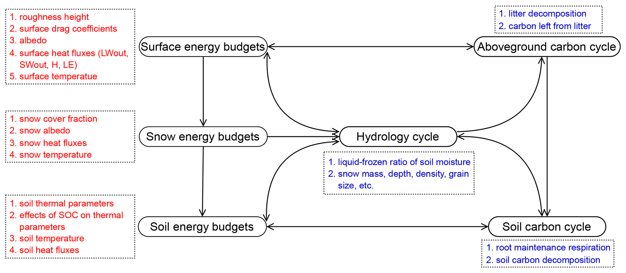
Figure 2 Modifications of energy, hydrology, and carbon processes to implement tiling energy budgets in ORCHIDEE-MICT in this study. The black oblongs show the main modules in ORCHIDEE-MICT, and the dashed rectangles containing red or blue text show the processes that are modified to include the multi-tilling energy budget. Here, red and blue differentiate between the respective processes in which the PFT-specific calculations are added actively and those modified passively due to the input variables changing following the multi-tilling surface, snow, and soil thermodynamics.

3 Implementation of tiling energy budgets in ORCHIDEE-MICT-teb

To represent the sub-grid energy budget in MICT, we calculate PFT-specific surface properties, including the roughness height and the albedo of different PFTs, to start the separation of surface energy budgets for each PFT; we then add the PFT-specific calculation for energy budget at the surface as well as in the snow and soil layers (Figs. 1, 2). As we use distinct input variables from the energy budget module, some processes in the hydrological cycle and carbon cycle are also modified correspondingly. The details of all of the modifications are given in the following.

3.1 Surface energy budgets

Differences in surface properties serve as the foundation for distinct surface energy budgets across sub-grids. For example, variations in vegetation heights among tree, grass, and bare-soil land cover types result in different aerodynamic roughness, drag coefficients, and then turbulent fluxes, including H and LE (Eqs. 3, 4). Different surface types among tree, grass, and bare-soil land cover types also result in different surface albedo (α), influencing the amount of solar radiation reflected by the surface (Eq. 2). In MICT-teb, we employ the specific roughness height (H_rough, the vegetation height minus the zero-plane displacement height) and albedo for each PFT (Tables S1, S3, and S4 and Fig. S1 in the Supplement), instead of the average values of all PFTs within a grid cell used in MICT. Thus, if only considering the changes in surface properties, the more heterogeneous the sub-grid PFT distribution, the larger the possible differences in the energy and the subsequent hydrology and carbon-related processes between MICT-teb and MICT. The distinct surface properties among different PFTs propagate to differences in surface energy fluxes and then differentiate the T_surf across different PFTs. In MICT-teb, all processes related to the changes in surface properties and T_surf in the surface energy budget are separated and operate independently for each PFT (Fig. 2).

For LE (or ET), it comprises four components in the model: E_subli, E_soil, E_trans, and E_inter. As described in Sect. 2.1, only E_trans and E_inter are PFT-specific in the original MICT. However, due to the modifications made to surface energy budgets and surface properties, resulting in varying snow cover fractions across different PFTs, E_subli is now separated for each PFT in MICT-teb. Regarding E_soil, the water limitation in the hydrology module differs among different soil tiles, whereas it is considered at the grid scale only in MICT. The calculation of E_soil has been modified using the specific water limitation for each soil tile in MICT-teb. All PFTs in one soil tile are assigned the same value of E_soil and are then used in PFT-specific calculation in energy modules.

3.2 Snow energy budgets

The modifications to the surface energy budget in MICT-teb, which cause variations in heat fluxes into the snowpack, result in differences in the formation and melting of snow and, in turn, snow mass, snow depth (dz_snow), and snow density (ρ_snow) among different PFTs. The snow cover fraction (f_snow), as calculated in MICT, is as follows (Niu and Yang, 2007; Wang et al., 2015):

$$\begin{array}{}\text{(11)}& \begin{array}{rl}{f}_{\text{snow}}=& \tanh \left({\sum }_{i=\mathrm{1}}^{\mathrm{3}}\right({\text{dz}}_{\text{snow},i})/\mathrm{0.025}\\ & \times \left({\sum }_{i=\mathrm{1}}^{\mathrm{3}}\right({\text{dz}}_{\text{snow},i}\cdot {\mathit{\rho }}_{\text{snow},i})\\ & /{\sum }_{i=\mathrm{1}}^{\mathrm{3}}\left({\text{dz}}_{\text{snow},i}\right))/\mathrm{50}).\end{array}\end{array}$$

This value would be different for different PFTs. In the above expression, i is the index of snow layer. The variations in f_snow would subsequently influence the surface albedo due to snow (Eq. 10) and, in turn, the snow feedbacks on the surface energy budget. All of the snow-related processes have been separated for each PFT in MICT-teb (Fig. 2).

3.3 Soil energy budgets

Following Eq. (5), modifications of energy budgets at the surface and in snow layers could result in variations in the starting point of heat conduction in soil for different PFTs. While within the soil, the heat conduction is more regulated by the heat capacity (c) and thermal conductivity (λ). Liquid SM, frozen SM, and SOC are three key factors influencing the two thermal parameters in the model (Eqs. 6, 7). In the original MICT model, the average values of these three factors across all PFTs are used due to the limitation of having a grid-scale mean energy budget. In the new version, we simulate PFT-specific liquid SM and frozen SM in energy modules to represent the heterogeneity of different PFTs, following the separation of soil heat conduction (Fig. 2). Regarding SOC, MICT uses the grid cell SOC obtained from an observation-based SOC map (FAO, 2012; Zhu et al., 2019; Guimberteau et al., 2018; Hugelius et al., 2013); therefore, the effects of SOC on thermal parameters are represented homogeneously within each grid cell. According to Zhu et al. (2019), an increase of 20 kg C m⁻³ in SOC between two PFTs, which can be found in site-level data (Palmtag et al., 2022) and is reproduced in model simulations (Fig. S2 in the Supplement), could result in a 42 %–52 % decrease in thermal diffusivity ($\mathit{\lambda }/c$) and a subsequent 13 %–18 % increase in the current permafrost extent. The important role of SOC in regulating soil thermal regimes and the heterogeneity of SOC across different PFTs highlight the pressing need to represent the thermal effects of SOC for each sub-grid. However, limited by the availability of observed SOC data that could be prescribed for sub-grids at the regional or global scale, we utilize the simulated SOC for each PFT in MICT-teb and the simulated total SOC of all PFTs in MICT. Using simulated instead of prescribed SOC has the advantage of making the modeled SOC fully consistent with the simulated soil physics, but it has the drawback that SOC formed by processes that cannot be simulated by the model (e.g., Pleistocene ecosystems such as yedoma, thermokarst lakes filling by organic sediments) will be ignored, causing a possible mismatch with observed SOC density. Nevertheless, a comparable spatial pattern of gridded SOC for 0–3 m over the Northern Hemisphere (NH) against observation-based SOC data and a comparable vertical profile against site-level data (Palmtag et al., 2022) confirm the model's ability to simulate the total volume (Fig. S3 in the Supplement) and the PFT-specific vertical profiles (Fig. S2 in the Supplement) of SOC.

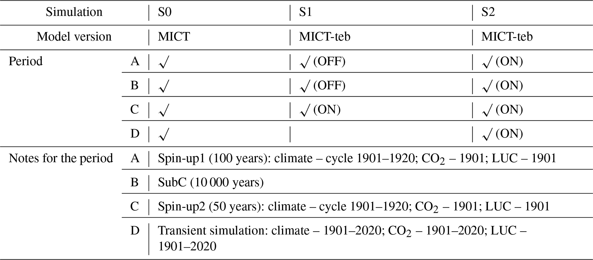
Table 1 Simulation protocol. MICT and MICT-teb indicate the original ORCHIDEE-MICT (without tiling energy budget) and the new ORCHIDEE-MICT-teb (with tiling energy budget), respectively. OFF and ON indicate turning the flags that control the tiling energy budget in MICT-teb off and on, respectively. If the flags are turned off, all of the PFT-specific variables related to energy budget will use the grid cell mean value in MICT-teb. LUC indicates land use change.

3.4 Associated modifications of hydrological and carbon processes

Soil temperature (T_soil) is a key factor that influences hydrological and biogeochemical processes in the soil. Therefore, the PFT-specific variations in T_soil result in a series of associated modifications to the hydrological and carbon-related processes with respect to the original MICT model (Fig. 2). For soil hydrology, there are three main modifications in MICT-teb compared with MICT: (1) the calculation of PFT-specific T_soil for each PFT to calculate the liquid-to-frozen phase ratio of SM, (2) the use of PFT-specific bare-soil evaporation from the energy module, and (3) the separation of snow-related processes for each PFT. For the soil carbon cycle, there are four main modifications in MICT-teb: (1) the use of PFT-specific T_soil and SM for litter decomposition, (2) the use of PFT-specific T_soil and SM to calculate carbon flow from litter to soil, (3) the use of PFT-specific T_soil and SM for root maintenance respiration, and (4) the use of PFT-specific T_soil and SM for soil carbon decomposition.

4 Simulation protocol and forcing datasets

To compare the differences in energy, hydrology, and carbon processes between MICT-teb and MICT, we design three groups of simulations (S0, S1, and S2), as shown in Table 1. All of the three groups are run for the NH (0–90° N) at a 2° × 2° spatial resolution with four simulation periods: (A) Spin-up1 – 100 years of the full ORCHIDEE model with a looped 1901–1920 climate, the CO₂ level of 1901 at 296.80 ppm, and the land cover map of 1901; (B) SubC – 10 000 years of the soil carbon sub-model to accumulate SOC; (C) Spin-up2 – 50 years of the full ORCHIDEE model to reach equilibrium with a looped 1901–1920 climate, the CO₂ level of 1901, and the land cover map of 1901; and (D) Transient simulation – the full ORCHIDEE model with varying climate and the CO₂ level and land cover maps from 1901 to 2020. The climate forcing data are obtained from CRU-JRA v2.3 (the version used in Global Carbon Budget 2022) (Friedlingstein et al., 2022), while the land cover maps are generated by combining the land cover map from TRENDY for 15 PFTs (bare soil, 8 tree PFTs, 4 grass PFTs, and 2 crop PFTs) (Lurton et al., 2020) and the peat map from Xu et al. (2018) for the peat grass PFT (Xu et al., 2018; Qiu et al., 2019). In S0, the original MICT model is used for all four periods. In S1, MICT-teb is used with the flags controlling the tiling energy budget (TEB) turned off for periods A and B (i.e., identical to group S0) but turned on for period C. In this way, the differences in energy, hydrology, and carbon between S0 and S1 solely due to the TEB can be compared based on the same starting point (end of period B). In S2, the flags controlling the TEB are turned on from the beginning of period A. Thus, comparing S0 and S2 could infer differences in the long-term equilibrium of energy and hydrology as well as the near-equilibrium soil carbon storage between MICT-teb and MICT.

5 Evaluation of the impacts of the tiling energy budget on energy, hydrology, and carbon processes

Following the description of the simulation protocol in Sect. 4, this section presents the differences in energy, hydrology, and carbon processes between MICT-teb and MICT. Section 5.1 presents the comparison of S1 and S0, i.e., the impacts solely due to TEB, while Sect. 5.2 presents the comparison of all the three simulations across the first three simulation periods, i.e., the long-term impacts of the TEB on energy, hydrology, and carbon processes. Unless otherwise stated, all differences indicate the mean values of the last 10 years in period C from MICT-teb minus those from MICT in Sect. 5.1.

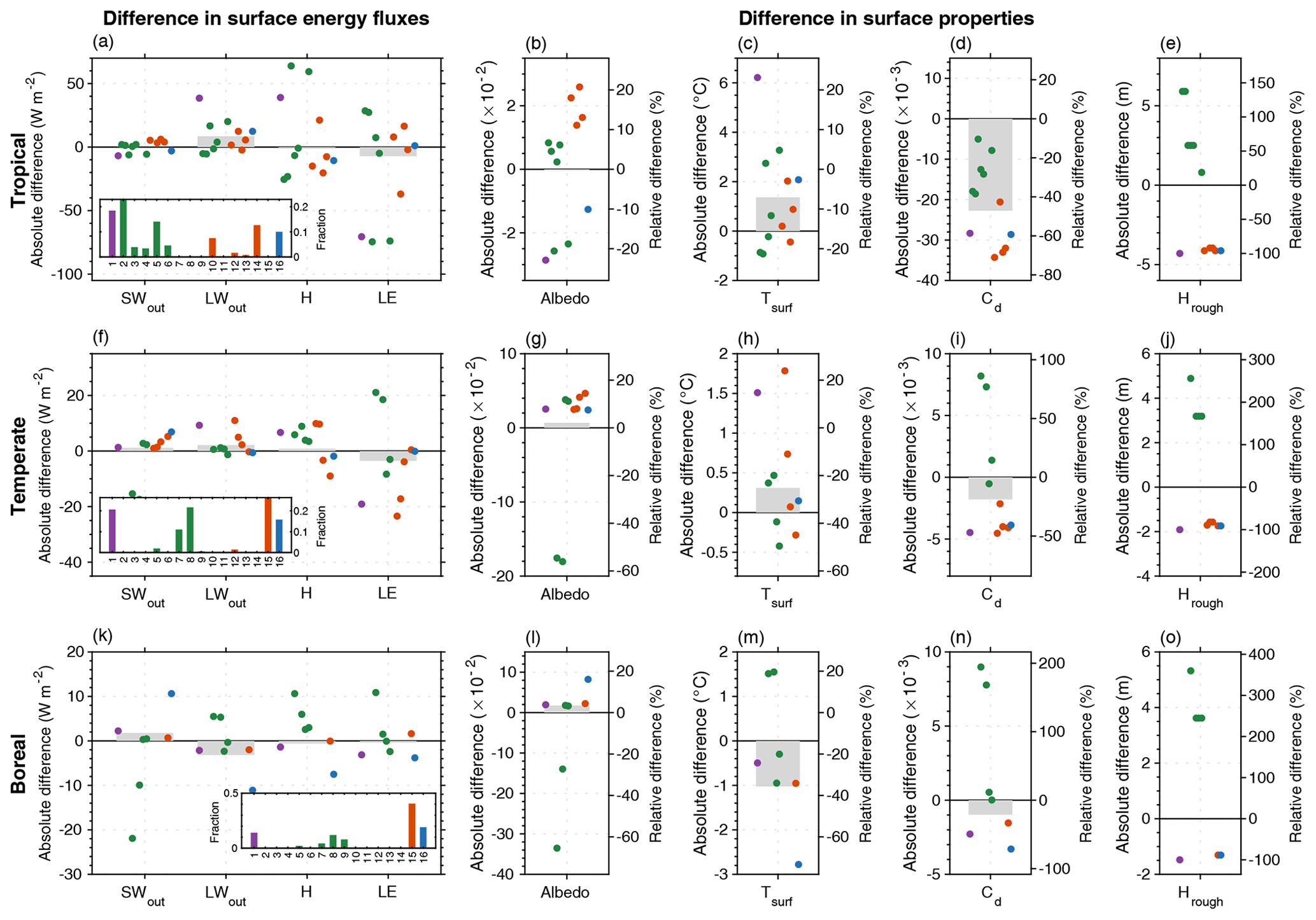
Figure 3 Differences in surface energy fluxes (the first column) and surface properties (from the second to the last column) between MICT-teb and MICT for three grid cells located in the tropical (17° N, 155° W), temperate (51° N, 101° W), and boreal (71° N, 147° E) regions, respectively. The surface energy fluxes include outward shortwave radiation (SW_out), outward longwave radiation (LW_out), sensible heat flux (H), and latent heat flux (LE). The surface properties include albedo (Albedo), surface temperature (T_surf), surface drag coefficient (C_d), and roughness height (H_rough). The gray bar in the background indicates the grid-scale difference in each variable. The colored points from left to right indicate the differences between 16 PFTs in MICT-teb and the grid-scale values in MICT, and the missing points indicate that the cover fraction of 1 PFT is 0 for the grid cell. The insets in the first column show the cover fraction of 16 PFTs for the grid cell. The 16 PFTs are bare soil (PFT 1, in purple), trees (PFT 2–9, in green), grass (PFT 10–15, in orange), and peat grass (PFT 16, in blue). The reader is referred to Table S3 for the full names of the 16 PFTs.

5.1 Impacts solely due to the tiling energy budget

5.1.1 Surface energy budgets

To explain the differences in energy budgets between MICT-teb and MICT, we begin our analysis by randomly selecting three grid cells at latitudes for tropical (17° N, 155° W), temperate (51° N, 101° W), and boreal (71° N, 147° E) biomes (Fig. 3). For the energy budgets at the surface (Eq. 2), the SW_in and LW_in are the same between the two versions (not shown), as both variables come from the input climate data, whereas the other four main surface energy fluxes, including SW_out, LW_out, H, and LE, show significant differences due to the TEB. The differences in energy fluxes can be well explained by the differences in surface properties at all three grid cells for the different latitudes. For instance, the difference in SW_out between MICT-teb and MICT can be explained by the difference in albedo, the difference in LW_out can be explained by the difference in T_surf, and the difference in H (or LE) can be explained by the difference in T_surf and/or C_d (surface drag coefficients). This correlation agrees well with theoretical equations (Eqs. 2–4).

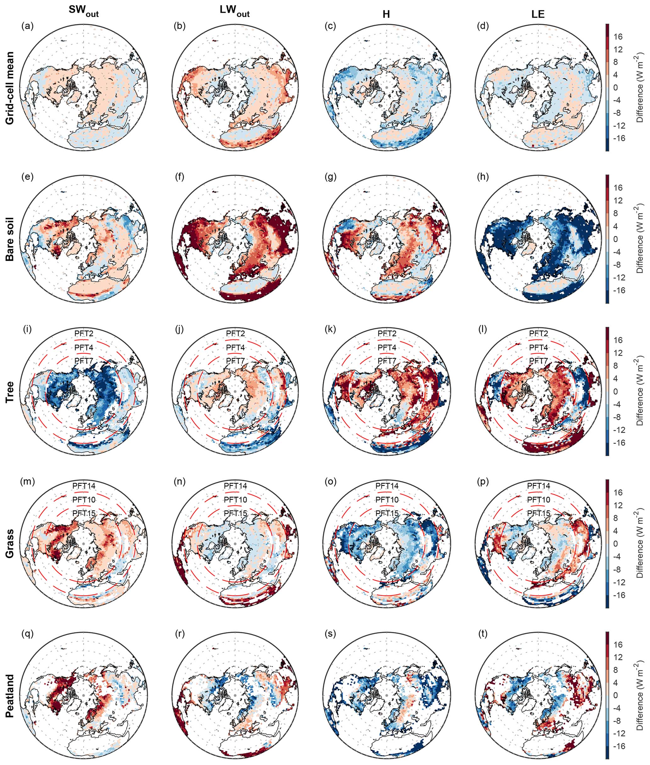
Figure 4 Spatial patterns of differences in surface energy fluxes including outward shortwave radiation (SW_out), outward longwave radiation (LW_out), sensible heat flux (H), and latent heat flux (LE) between MICT-teb and MICT over the Northern Hemisphere. The first to fifth rows show the difference in each flux between the grid cell mean (a–d) or four tiles (e–t) from MICT-teb and the grid cell mean from MICT, respectively. The four tiles include (e–h) bare soil (PFT1), (i–l) tree (a combination of PFT2 (tropical broad-leaved evergreen tree) south of 20° N, PFT4 (temperate needleleaf evergreen) between 20 and 40° N, and PFT7 (boreal needleleaf evergreen tree) north of 40° N), (m–p) grass (a combination of PFT14 (Topical C₃ grass) south of 20° N, PFT10 (temperate C₃ grass) between 20 and 40° N, and PFT15 (boreal C₃ grass) north of 40° N), and (q–t) peatland grass (PFT16). The three PFTs for the tree or grass are combined in order to show as many results as possible, but only one PFT is shown in each grid cell.

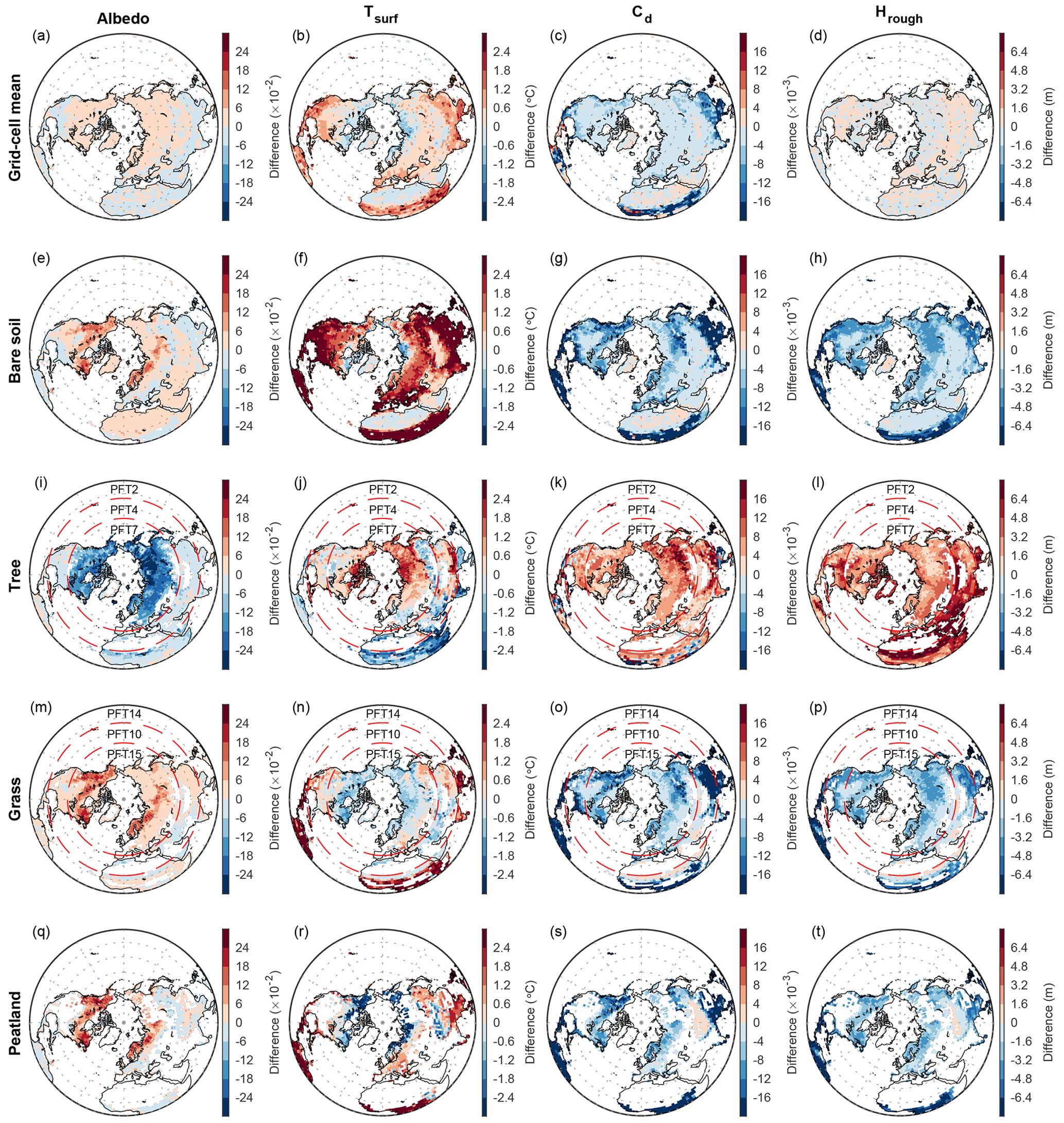
Figure 5 Same as Fig. 4 but for spatial patterns in the differences in surface properties, including albedo (Albedo), surface temperature (T_surf), surface drag coefficients (C_d), and roughness height (H_rough) between MICT-teb and MICT over the Northern Hemisphere.

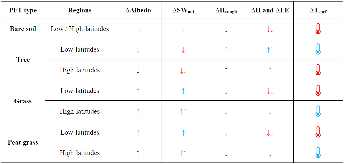
Table 2 Qualitative summary of latitudinal trends in the differences in surface properties and associated differences in surface energy fluxes between MICT-teb and MICT. The red and blue arrows indicate the warming and cooling effects on surface temperature, respectively. Two arrows indicate a stronger effect than one arrow.

The variations in surface properties are related to the modifications made to represent the PFT-specific information in MICT-teb. Regarding albedo, grass leaves generally have a higher albedo (0.15–0.16) than tree leaves (0.10–0.14) (Table S1 in the Supplement), while the albedo of bare soil varies in the model depending on soil moisture, ranging from ∼ 0.05 in moist areas to ∼ 0.5 in dry areas (Fig. S1 in the Supplement). In the tropical grid cell, all four grass PFTs show a higher albedo than the grid cell mean (0.125); in contrast, some of the six tree PFTs show a lower albedo than the grid cell mean, whereas others show a higher value. The peat PFT has the same leaf albedo value as grass PFTs, but its albedo, as shown in Fig. 3b, is lower than the grid cell mean, which is due to the higher fraction of bare soil (with a small albedo of 0.093) for this PFT (∼ 70 %) relative to the other four grass PFTs (2 %–30 %). We note that the cover fraction of a PFT in the model includes both the leaf-covered area (the canopy) and the non-leaf-covered area (the soil), depending on a function of the leaf area index. The albedo of a PFT is calculated as the area-weighted sum of the albedo of leaves and the albedo of soil within this PFT. In temperate and boreal regions, the albedo of one PFT is greatly influenced by the snow cover fraction, owing to the significantly higher albedo of snow (Table S3). Consequently, the pattern of the difference in albedo between MICT-teb and MICT (Fig. 3g, l) closely resembles the difference in the snow cover fraction (Fig. S4 in the Supplement) for temperate and boreal grid cells. Regarding C_d, the surface drag coefficient, its variation is determined by the variation in the PFT-specific T_surf and H_rough (roughness height): the smaller the T_surf and the larger the H_rough, the larger the C_d. The theoretical relationship can be reproduced well from the comparison of simulated results between MICT-teb and MICT in Fig. 3.

When extending this to the whole NH, the correspondence between differences in surface heat fluxes and differences in surface properties at the grid cell scale can still be observed (Figs. 4 and 5 as well as Fig. S5 in the Supplement). Additionally, certain latitudinal trends begin to emerge in the difference between MICT-teb and MICT. Based on our modifications to calculate PFT-specific leaf albedo and H_rough, the most immediate variations in SW_out or turbulent fluxes (H and LE) lead to the final direction of differences in T_surf between MICT-teb and MICT for different PFTs (Table 2). For bare soil, whose H_rough is set to 0 in MICT-teb, the smaller H and LE result in a higher T_surf (up to 3 °C) compared with MICT across almost all areas with bare soil. For tree PFTs, the higher H and LE due to the larger H_rough contribute to an overall cooler T_surf (−3 to 0 °C) at low latitudes, while the more important decrease in SW_out due to the smaller albedo in MICT-teb results in a warmer T_surf (0–2 °C) at high latitudes. With the same dominant role of the H_rough variation at low latitudes and of the albedo variation at high latitudes, the grass and peat grass show a warmer T_surf (0–3 °C) at low latitudes but a cooler T_surf (−1 to 0 °C for grass and −2 to 0 °C for peat grass) at high latitudes in MICT-teb. As a result, the grid cell T_surf simulated by MICT-teb is 0–2 °C higher in most regions in the NH, although it is slightly cooler (−1 to 0 °C) north of 60° N and in some arid regions compared with MICT (Fig. 5b).

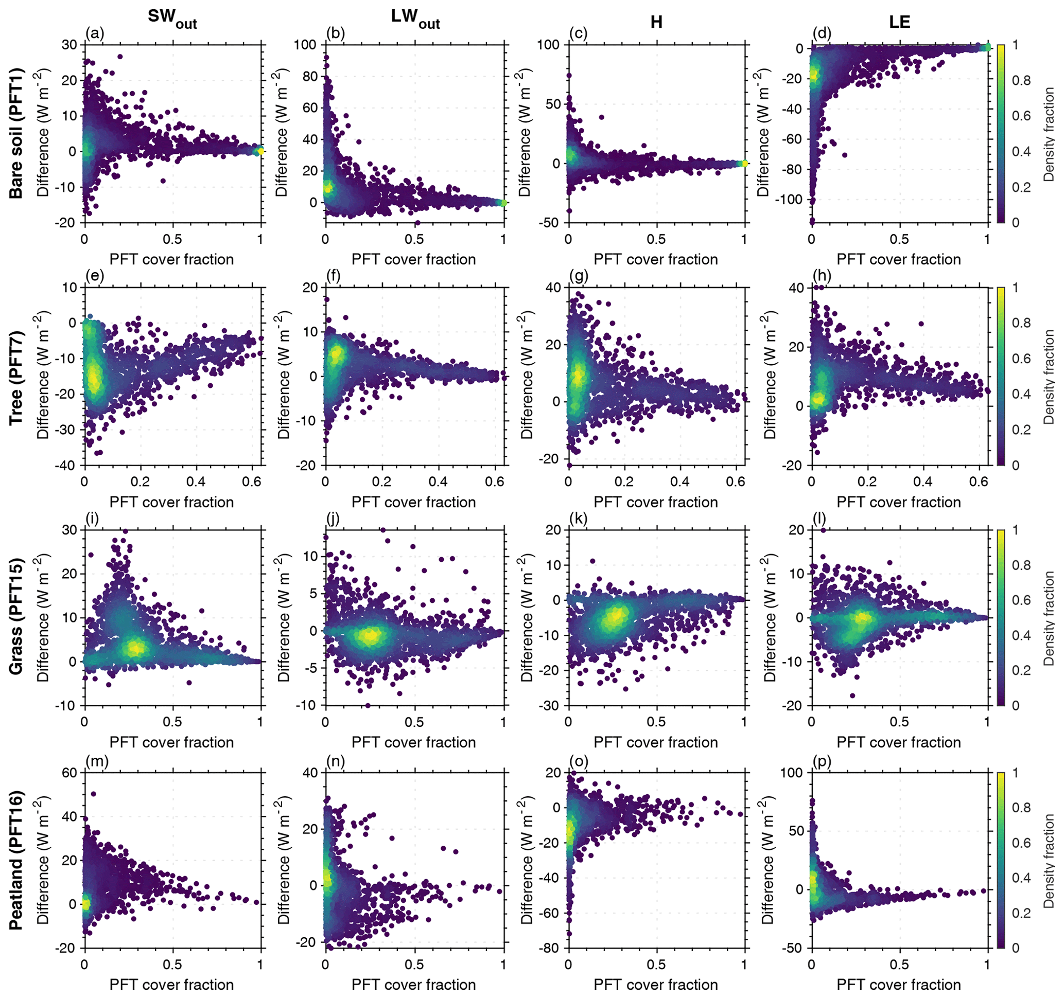
Figure 6 Scatterplot of differences in surface energy fluxes between MICT-teb and MICT versus the vegetation cover fraction for bare soil (PFT1), tree (PFT7), grass (PFT15), and peatland grass (PFT16) plant functional types. The surface energy fluxes include outward shortwave radiation (SW_out), outward longwave radiation (LW_out), sensible heat flux (H), and latent heat flux (LE). The color of each point represents the density fraction of grid cells.

Another interesting result is the relationship between differences in surface heat fluxes or properties between MICT-teb and MICT and the vegetation cover fraction. As mentioned in Sect. 3.1, the difference between the two versions should become smaller in areas where one PFT tends to become more dominant in the grid cell. When the cover fraction of one PFT approaches 100 %, there will be no difference between the grid cell mean and the specific PFT. Taking four PFTs as examples, we found this pattern for both the surface heat fluxes (Fig. 6) and surface property variables (Fig. S6 in the Supplement).

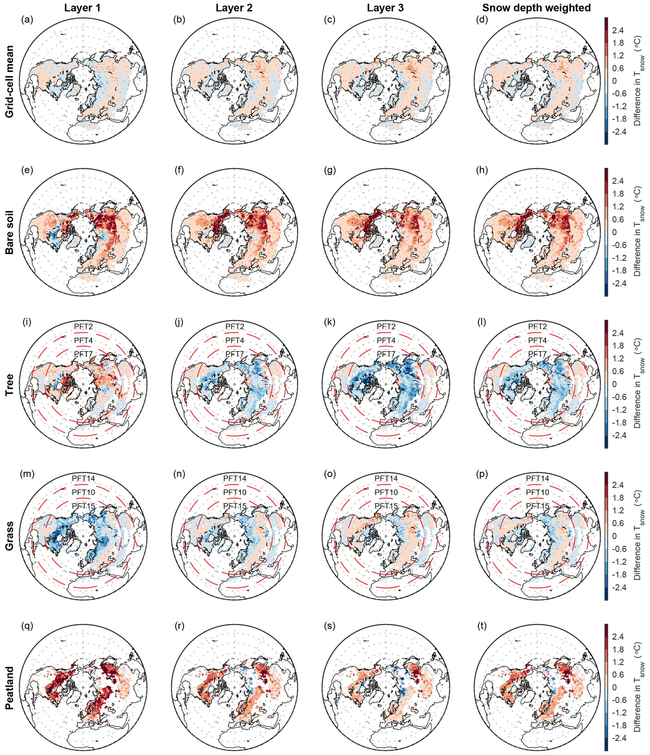
Figure 7 Spatial patterns in the difference in T_snow between MICT-teb and MICT for three snow layers and the snow-depth-weighted results over the Northern Hemisphere. The snow layers from top to bottom are numbered 1, 2, and 3, respectively. The snow-depth-weighted results are shown due to the different snow layer depth across different grid cells.

5.1.2 Snow energy budgets

Figure 7 presents differences in T_snow (ΔT_snow) for three snow layers between MICT-teb and MICT for the grid cell mean and four PFTs. Overall, the grid cell ΔT_snow follows the ΔT_surf between the two versions, with a snow layer that is up to 1 °C warmer across most areas in MICT-teb. The correlation of ΔT_snow and ΔT_surf weakens from the uppermost snow layer (T_snow,1) to the bottom one (T_snow,3), especially for the tree and grass PFTs (Table S5 in the Supplement). For the two aforementioned PFTs, the differences in the two thermal parameters (c_snow and λ_snow) play a more important role than ΔT_surf in shaping the spatial pattern of ΔT_snow in the bottom two layers (Table S5 and Figs. S7 and S8 in the Supplement). As the snow depth for each layer is not fixed like soil layers (Fig. 1), we calculate the snow-depth-weighted ΔT_snow between the two versions (the last column in Fig. 7). The differences in c_snow and λ_snow are more important in determining the spatial patterns of the snow-depth-weighted ΔT_snow.

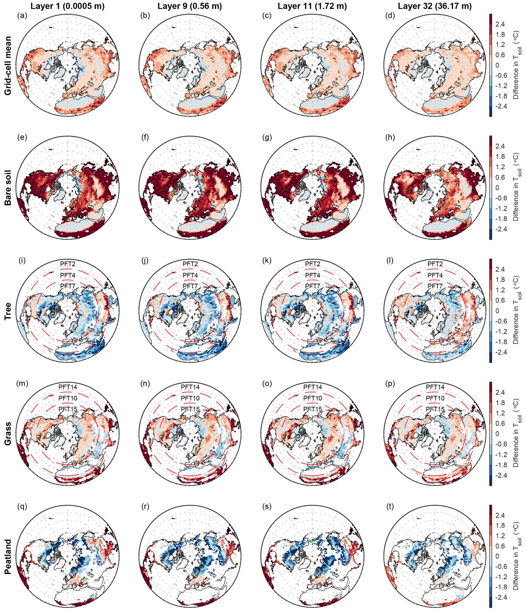
Figure 8 Same as Fig. 7 but for spatial patterns in the differences in T_soil between MICT-teb and MICT for four soil layers over the Northern Hemisphere.

5.1.3 Soil energy budgets

Figure 8 presents the differences in T_soil (ΔT_soil) of four soil layers between MICT-teb and MICT for the grid cell mean and four PFTs. Similar to ΔT_snow, ΔT_soil shows a larger and significantly positive correlation (R = 0.31–1.00, p < 0.05) with differences in the starting point of heat conduction (T_surf for 0–30° N and T_snow,3 for 30–90° N) compared with the two thermal parameters of soil (Table S6 in the Supplement). The grid cell mean T_soil for the four soil layers simulated by MICT-teb is ∼ 0.6 °C warmer than MICT north of 30° N, whereas it is ∼ 1.2 °C warmer in the tropics across four soil layers. The PFT-specific ΔT_soil values show considerably different magnitudes and directions across the four PFTs: the T_soil for bare soil is ∼ 3 °C higher in MICT-teb than in MICT, the T_soil for tree and peat grass PFTs is 0.6–3 °C lower, and the T_soil for grass is 0.6–3 °C higher. Despite using the same parameter values of leaf albedo and H_rough between peat grass and C₃ grass, the T_soil of peat grass is 0.6–3 °C lower at high latitudes in MICT-teb, which could be related to the considerably different spatial patterns of the two soil thermal parameters between peat grass and C₃ grass (Table S6 and Figs. S9 and S10 in the Supplement).

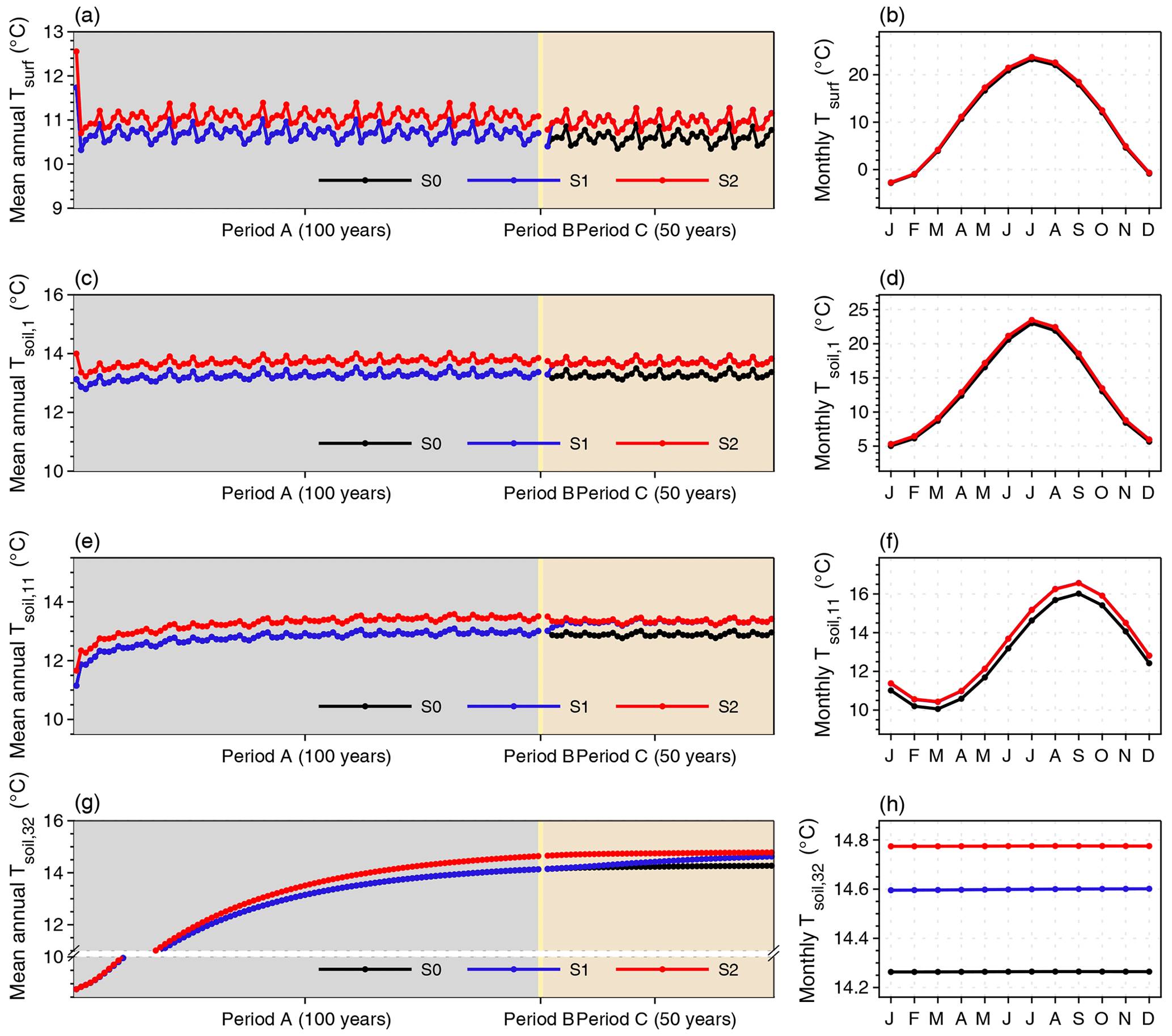
Figure 9 Time series and seasonal cycle of surface temperature (T_surf) and soil temperature for three soil layers (T_soil,1, T_soil,11, and T_soil,32) over the Northern Hemisphere from three simulations. The annual values are calculated using the yearly average, and the monthly values are calculated using the average of the last 10 years in period C. The backgrounds in panels (a), (c), (e), and (g) are shaded to help explain the simulation length of the three periods. Detailed explanations for the three simulations (S0, S1, and S2) and the three periods (A, B, and C) can be found in Table 1 and Sect. 4.

As mentioned in Sect. 3.3, the liquid SM (SM_liquid), frozen SM (SM_frozen), and SOC are three key factors influencing the two thermal parameters of soil (Eqs. 6 and 7). Despite the previous soil-tile-based hydrological processes and PFT-based carbon cycle in MICT, the soil thermal parameters (c and λ) are calculated with the grid cell mean values of SM_liquid, SM_frozen, and SOC in that version. With far wetter SM (≥ 200 %; Figs. S11 and S12 in the Supplement) and far more SOC storage (≥ 200 %; Fig. S13 in the Supplement), the peat PFT has a ∼ 200 % higher c (Fig. S9 in the Supplement) and a ∼ 100 % higher λ (Fig. S10 in the Supplement) than the grid cell mean. Such a large Δc and Δλ compared with grass (40 % higher/lower c and 20 % higher/lower λ than the grid cell mean) lead to a lower T_soil for peat grass in MICT-teb compared with MICT (Fig. 8). Besides the peat grass PFT, the important role of the three factors in regulating T_soil can also be found for other PFTs. For example, we found ∼ 100 % less SOC storage in bare soil than the grid cell mean, which contributes to the higher T_soil for bare soil due to the absence of the insulating impacts of SOC.

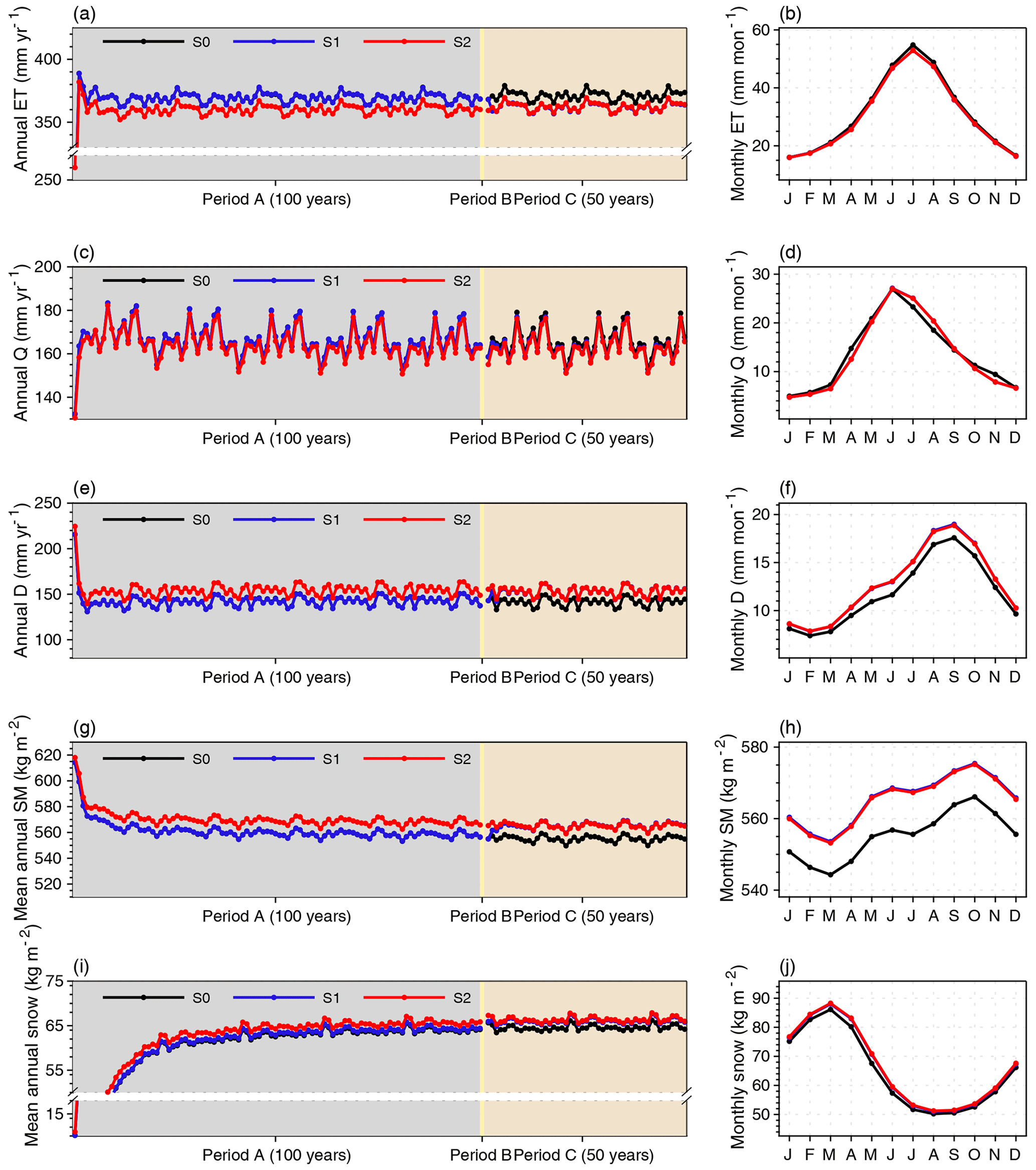
Figure 10 Time series and the seasonal cycle of hydrological variables including evapotranspiration (ET), surface runoff (Q), drainage (D), soil moisture (SM), and snow over the Northern Hemisphere from three simulations.

5.2 Long-term impacts on energy, hydrology, and the carbon cycle

5.2.1 Energy

Regarding the long-term impacts of representing the sub-grid energy budgets in the model, we compare the simulated results over the NH among S0, S1, and S2 from three aspects: energy budgets, hydrology, and the carbon cycle (Figs. 9–11). For the energy budgets, we found that the difference in T_surf over the NH between S1 and S0 or between S2 and S0 appears in the first 2–3 years and then remains stable throughout all three simulation periods (Fig. 9a). By the end of period C, the ΔT_surf over the NH between S2 and S0 remains at 0.37 °C (+3.5 %). A very similar ΔT_surf (0.38 °C, 3.6 %) can be observed between S1 and S0, suggesting that the surface energy budgets can quickly respond to variations in surface properties, including albedo and roughness. As the heat moves down, the determining role of T_surf with respect to influencing the heat conduction in soil (Table S6) makes the T_soil at the 1st (0.0005 m), 11st (1.72 m), and 32nd (36.17 m) layers over the NH warmer by 0.44 °C (3.3 %), 0.45 °C (3.5 %), and 0.51 °C (3.6 %), respectively, by the end of period C under S2 compared with under S0. However, it takes longer for T_soil to reach stability in the bottom soil layers than in the upper ones (Fig. 9c, e, g). The SOC, acting as an insulator, could regulate the soil thermodynamics, especially in summer (Zhu et al., 2019). Nevertheless, the difference in mean annual or monthly T_soil in all soil layers between S1 and S2 is very small – no more than 0.18 °C (1.2 %). Therefore, the long-term effects of the TEB on the surface or soil energy budgets over the NH are subtle in the simulations in this study.

Figure 11 Time series and seasonal cycle of carbon-related variables including gross primary productivity (GPP), net primary productivity (NPP), heterotrophic respiration (R_h), and soil organic carbon (SOC) over the Northern Hemisphere from three simulations. The depth for R_h and SOC is 0–38 m.

5.2.2 Hydrology

The hydrological processes over the NH can respond to the representation of sub-grid energy budgets as quickly as temperature, taking up to 5 years to reach the stability for both surface water fluxes, including evapotranspiration (ET) and surface runoff (Q), and subsurface water fluxes, such as drainage (D) (Fig. 10). Overall, MICT-teb shows a smaller ET (−8.7 mm yr⁻¹, −2.3 %) but a larger D (+11.8 mm yr⁻¹, 8.3 %) over the NH compared with MICT. When separating the subcomponents of ET and soil tiles, we found that the decreased ET is mainly contributed by the decreased E_trans (transpiration) from tree PFTs and the decreased E_subli (sublimation) from the grass PFTs, with values of −3.7 and −3.0 mm yr⁻¹ per grid cell over the NH, respectively (Fig. S14 in the Supplement). Spatially, the decreased E_trans values for tree PFTs are mainly distributed in tropical regions and eastern North America, while the decreased grass E_subli is located at high latitudes (Fig. S15 in the Supplement). Both of these decreases are related to the variations in surface properties (the decreased C_d and/or decreased T_surf) in MICT-teb (Fig. 5). As a result of the balance between the variations in ET and runoff, the SM (0–2 m) in MICT-teb is 9.9 kg m⁻² (1.8 %) wetter than in MICT over the NH (Fig. 10).

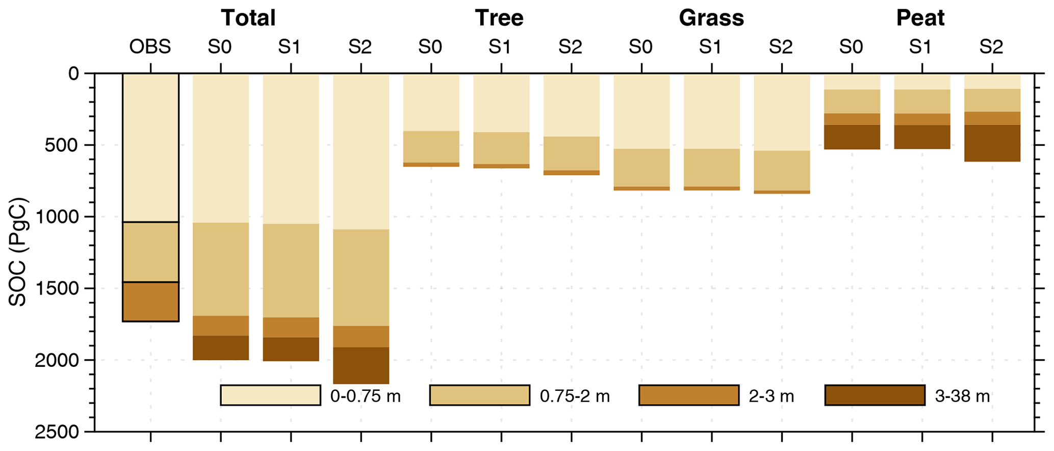
Figure 12 Vertical composition of soil organic carbon (SOC) for all PFTs and three vegetated soil tiles (tree, grass, and peat) over the Northern Hemisphere from an observation-based SOC map and three simulations. For observed data, we only show the results for all PFTs due to the lack of biome information. For simulations, all values are calculated using the average of the last 10 years in period C.

5.2.3 Carbon

In response to the warmer and wetter soils (Fig. S16 in the Supplement), vegetation productivity is significantly enhanced over the NH in MICT-teb, with a 1.9 Pg C yr⁻¹ (2.7 %) larger GPP and a 0.8 Pg C yr⁻¹ (2.7 %) larger NPP under S2 than S0 (Fig. 11). The enhanced productivity is primarily driven by tree PFTs across almost all NH regions and grass PFTs at middle and low latitudes, while the productivity of peatland grass is somewhat lower due to the cooler soil (Figs. S16 and S17 in the Supplement). The warmer soil also accelerates the heterotrophic respiration rate (R_h) for tree and grass PFTs, along with the variation in SM. Compared with S0, S2 has a larger SOC (+58.5 Pg C, 9.0 %) for tree PFTs but almost unchanged SOC storage (+22.5 Pg C, 2.8 %) for grass PFTs. Despite being the smallest SOC pool (∼ 27 %, ∼ 600 Pg C) (Hugelius et al., 2014, 2016, 2020; Lindgren et al., 2018) among the three vegetated soil tiles as a result of the small peatland area (∼ 3 % of vegetated land in the NH), the peatland PFT's SOC storage increases by 85.8 Pg C, accounting for more than a half of the total SOC increase from S0 to S2 (Fig. 12). The cooler soil throughout the entire vertical profile of the peat PFT promotes SOC accumulation by significantly slowing the soil respiration (R = 0.38, p < 0.01), showing a more critical role in regulating the SOC decomposition than SM (R = 0.20, p < 0.01). Moreover, unlike the energy and water processes, the difference in SOC (ΔSOC) over the NH between S2 and S0 is obviously larger than that between S1 and S0 (∼ 7 Pg C); from a temporal perspective, it exists after period B and then remains stable until the end of period C (Fig. 11g). This means that the ∼ 170 Pg C ΔSOC between S2 and S0 has accumulates from peat initiation, and the long-term effects of TEB on soil carbon cannot be neglected.

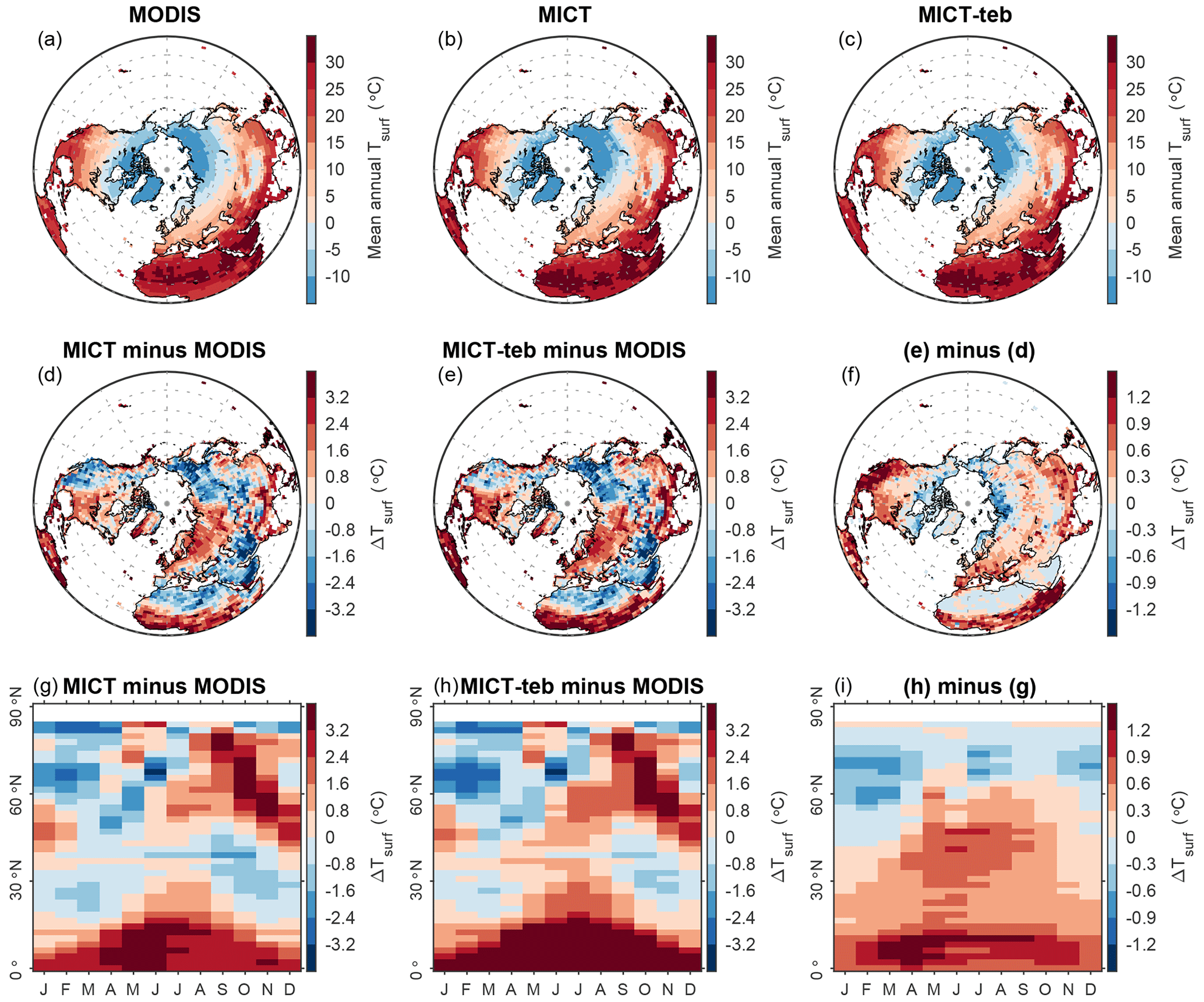
Figure 13 Evaluation of simulated surface temperature (T_surf) with land surface temperature (LST) from MODIS. (a–c) Spatial pattern of mean annual LST for 2001–2020 from MODIS, MICT, and MICT-teb. (d, e) Spatial pattern of the difference in mean annual T_surf for 2001–2020 between MICT (d) or MICT-teb (e) and MODIS. (f) Spatial pattern of the difference between panels (e) and (d). (g, h) Seasonal cycle of the difference in T_surf calculated over each latitude band between MICT (g) or MICT-teb (h) and MODIS. (i) Seasonal cycle of the difference between panels (h) and (g).

6 Evaluation and potential application

6.1 Evaluation of the simulated energy budgets

To evaluate the simulated surface energy budget, we compare the T_surf (surface temperature, mirroring outward longwave radiation and sensible heat flux), albedo (mirroring outward shortwave radiation), and LE (latent flux) from period D (Transient simulation, 1901–2020) with satellite-derived land surface temperature (LST), albedo, and LE from MODIS (the Moderate Resolution Imaging Spectroradiometer), respectively. The MODIS LST product is obtained from MOD11C3 Version 6.1 (https://lpdaac.usgs.gov/products/mod11c3v061/, last access: 3 July 2023), which records the monthly radiative skin temperature of the land surface at a 0.05° × 0.05° spatial resolution, spanning from 2000 to the present (Wan, 2013, 2014). Compared with the MODIS product, MICT and MICT-teb reproduce the spatial pattern of mean annual satellite-derived LST for 2001–2020 (Fig. 13a, b, c) but with an overestimation of up to 3 °C in wet regions, such as tropical regions, Europe, and eastern North America, as well as an underestimation of up to 3 °C in dry areas and northeastern Asia (Fig. 13d, e). Regarding the seasonality of T_surf, the two model versions show an overestimation of summer and autumn LST (by up to 3 °C) but an underestimation of winter LST (by up to 3 °C) at middle to high latitudes, while an overestimation of up to 3 °C exists throughout the year for the tropics (Fig. 13g, h). Including the representation of PFT-specific energy budgets alleviates the LST bias from MICT in some areas, such as western North America and northern Europe, and in some seasons, such as autumn at high latitudes, but it concurrently aggravates the LST bias in some areas and some seasons, such as all four seasons in tropical regions (Fig. 13f, i).

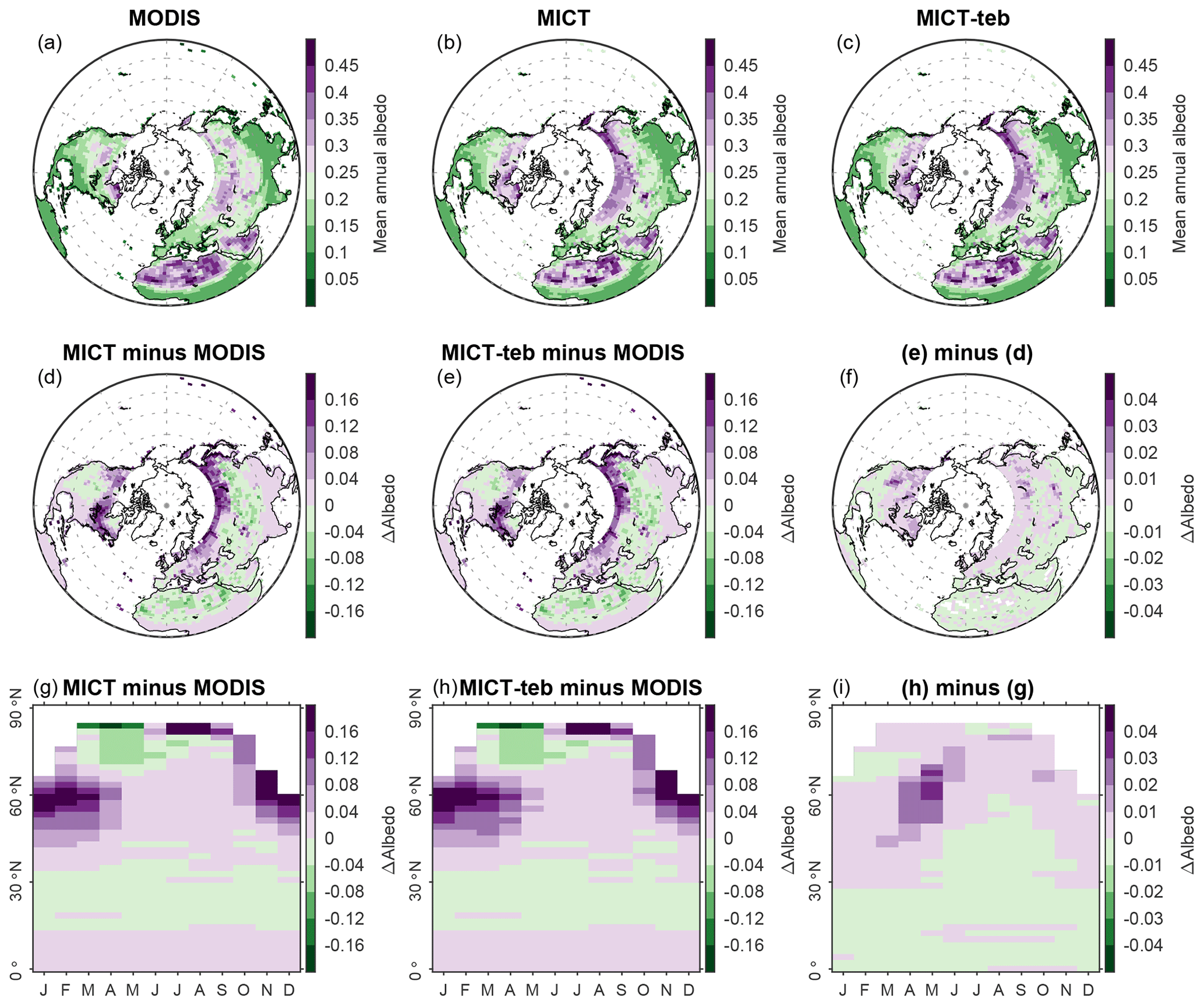
Figure 14 Same as Fig. 13 but for the evaluation of simulated albedo with blue-sky albedo from MODIS.

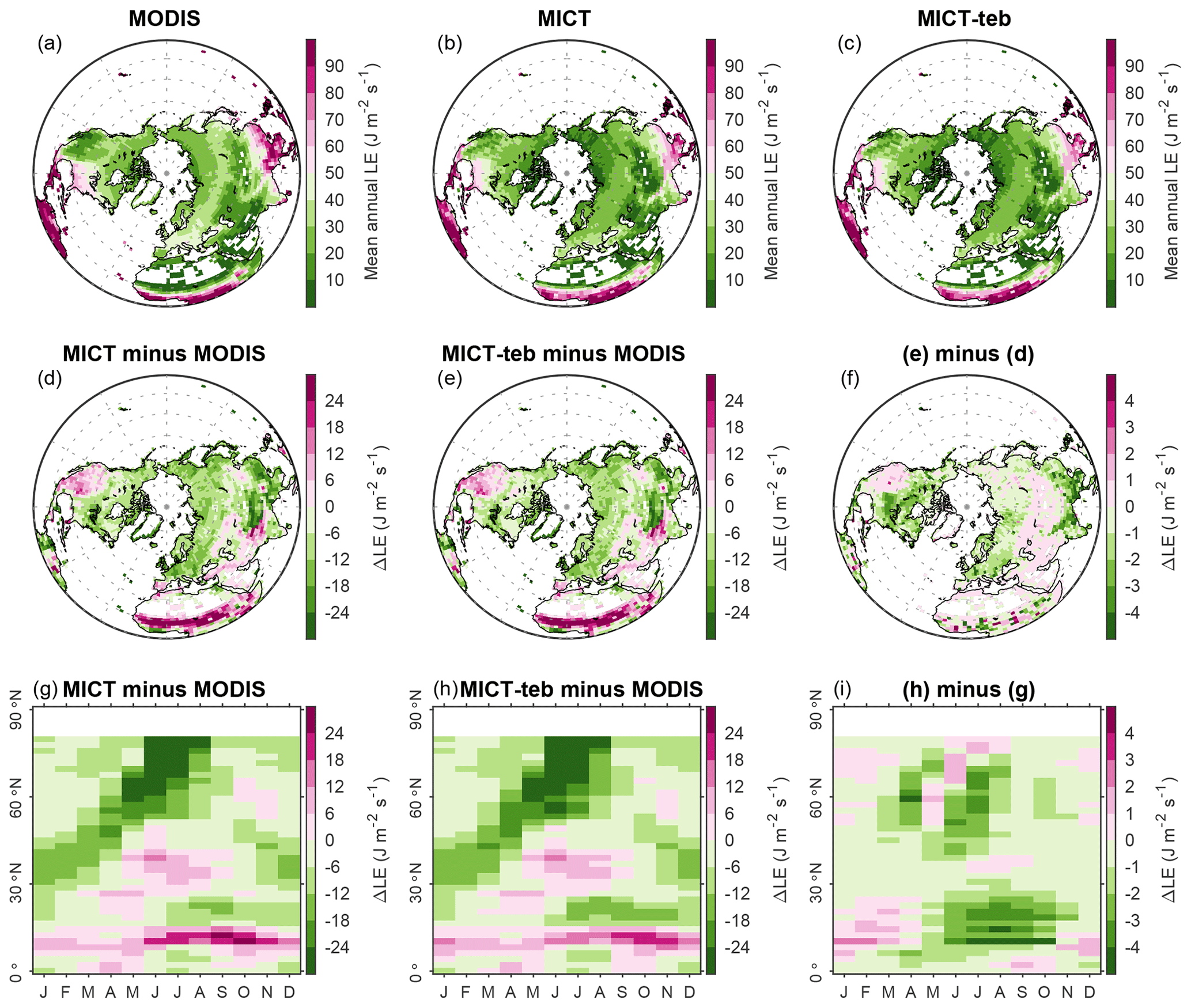
Figure 15 Same as Fig. 14 but for the evaluation of simulated latent flux (LE) with that from MODIS.

The MODIS albedo product is obtained from MCD43C3 Version 6.1 (https://lpdaac.usgs.gov/products/mcd43c3v061/, last access: 3 March 2024), including the daily black-sky and white-sky albedo at a 0.05° × 0.05° spatial resolution. For comparison with the albedo from the model, we calculate the blue-sky albedo using the black-sky and white-sky albedo for the shortwave band (0.3–5.0 µm) from MODIS, weighted by the diffuse skylight ratio derived from the direct and total shortwave radiation from the fifth-generation ECMWF reanalysis product (ERA5, https://cds.climate.copernicus.eu/cdsapp#!/dataset/reanalysis-era5-single-levels-monthly-means?tab=form, last access: 3 March 2024) (Hersbach et al., 2023). We found that, except for a ∼ 0.2 overestimation of winter and spring albedo in northern high latitudes, the simulated albedo from MICT and MICT-teb shows a very small bias, no more than 0.04 (Fig. 14). The considerable albedo biases in winter and spring could be related to the bias in the leaf area index and snow cover fraction values simulated by the model (Li et al., 2016). The MODIS LE product is obtained from MOD16A2GF Version 6.1 (https://lpdaac.usgs.gov/products/mod16a2gfv061/, last access: 3 March 2024), providing the 8 d LE at a 500 m × 500 m spatial resolution. Compared with the MODIS LE, the simulated LE tends to be smaller (−6 to −24 $\mathrm{J}{\mathrm{m}}^{-\mathrm{2}}{\mathrm{s}}^{-\mathrm{1}}$) in most areas except for some arid regions over the NH (Fig. 15). Same as the evaluation for T_surf, the representation of PFT-specific energy budgets does not reduce the albedo/LE biases significantly (panels g and h in Figs. 14 and 15).

There are several reasons that could explain disagreements in the surface energy budgets between the MODIS products and the models. On the one hand, (1) the under-representation of some important processes in the model, such as the parameterization of ET (LE) and snow insulation, as well as the uncertainties in climate forcing data (Guimberteau et al., 2018; Peng et al., 2016; Domine et al., 2016) and (2) missing data across dry areas and cloudy-weather days in the MODIS products, e.g., a ± 2 °C LST bias compared with ground-truth data found in dry areas (Li et al., 2014; Wan, 2014; Westermann et al., 2012), could partly account for disagreements between the MODIS products and the models. On the other hand, the considerably different land cover maps used by MODIS and the simulations (Fig. S18 in the Supplement) as well as the difference in one specific variable from MODIS and the simulations could contribute to the systematic biases or gaps. For instance, the LST from MODIS more closely reflects the radiative skin temperature, i.e., canopy temperature, while the canopy energy budget is absent in ORCHIDEE-MICT, which could result in a higher T_surf from the models compared with the MODIS LST in forest ecosystems (Fig. 13) (Gomis-Cebolla et al., 2018).

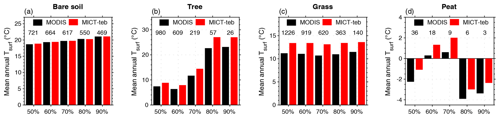
Figure 16 Evaluation of simulated surface temperature (T_surf) with land surface temperature (LST) from MODIS by PFT. (a–d) Mean annual T_surf for four PFTs (bare soil, tree, grass, and peat) for 2001–2020. The grid cells for each PFT are selected with five threshold fractions (50 %, 60 %, 70 %, 80 %, and 90 %), i.e., the minimum fractional coverage of one land cover type in the grid cell. The numbers of grid cells for each group of bars are shown.

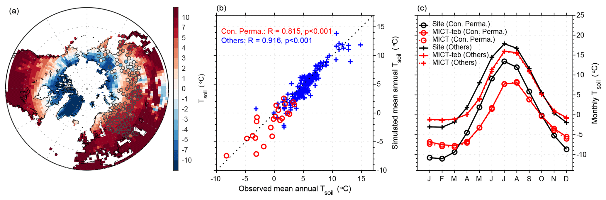
Figure 17 Evaluation of simulated soil temperature (T_soil) at 20 cm with site observations. (a) Spatial patterns of mean annual T_soil at 20 cm during the 1980–2000 period from the simulation of MICT-teb, with the values of 199 sites shown as color-filled circles. (b) Simulated (from MICT-teb) versus observed mean annual T_soil at 20 cm across all sites. (c) Mean seasonal cycle of site-averaged T_soil at 20 cm from site observations, MICT-teb, and MICT. The sites in panels (b) and (c) are divided into those located in continuous permafrost (Con. Perma.) regions (22 sites, circle markers) and others (177 sites, cross markers) according to the permafrost map of Brown et al. (2002).

In light of the new feature of MICT-teb to simulate PFT-specific energy budgets, we compare the simulated and satellite-based T_surf over grid cells dominated by four PFTs: bare soil, tree, grass, and peatland from simulations (Fig. 16). Despite the significant disagreements regarding the surface energy budgets between the MODIS products and the models, the model can produce a comparable T_surf to MODIS for the four PFTs. Moreover, the model can capture the variations in the LST from MODIS well when altering the threshold fractions for grid cell selection from 50 % to 90 %. For tree, grass, and peat, due to their extensive coverage in wet areas, the simulated T_surf is 1–3 °C warmer than the grid cell LST from MODIS for all threshold fractions. For bare soil, the underestimation of T_surf in desert areas is offset by the overestimation in Greenland (Fig. 13d, e). The notable biases when using a 90 % threshold fraction, a near-complete coverage of one PFT within one grid cell, suggests that the disagreement between the model and satellite products should be attributed to the gap between MODIS and the original version, rather than the separation of PFT-specific energy budgets.

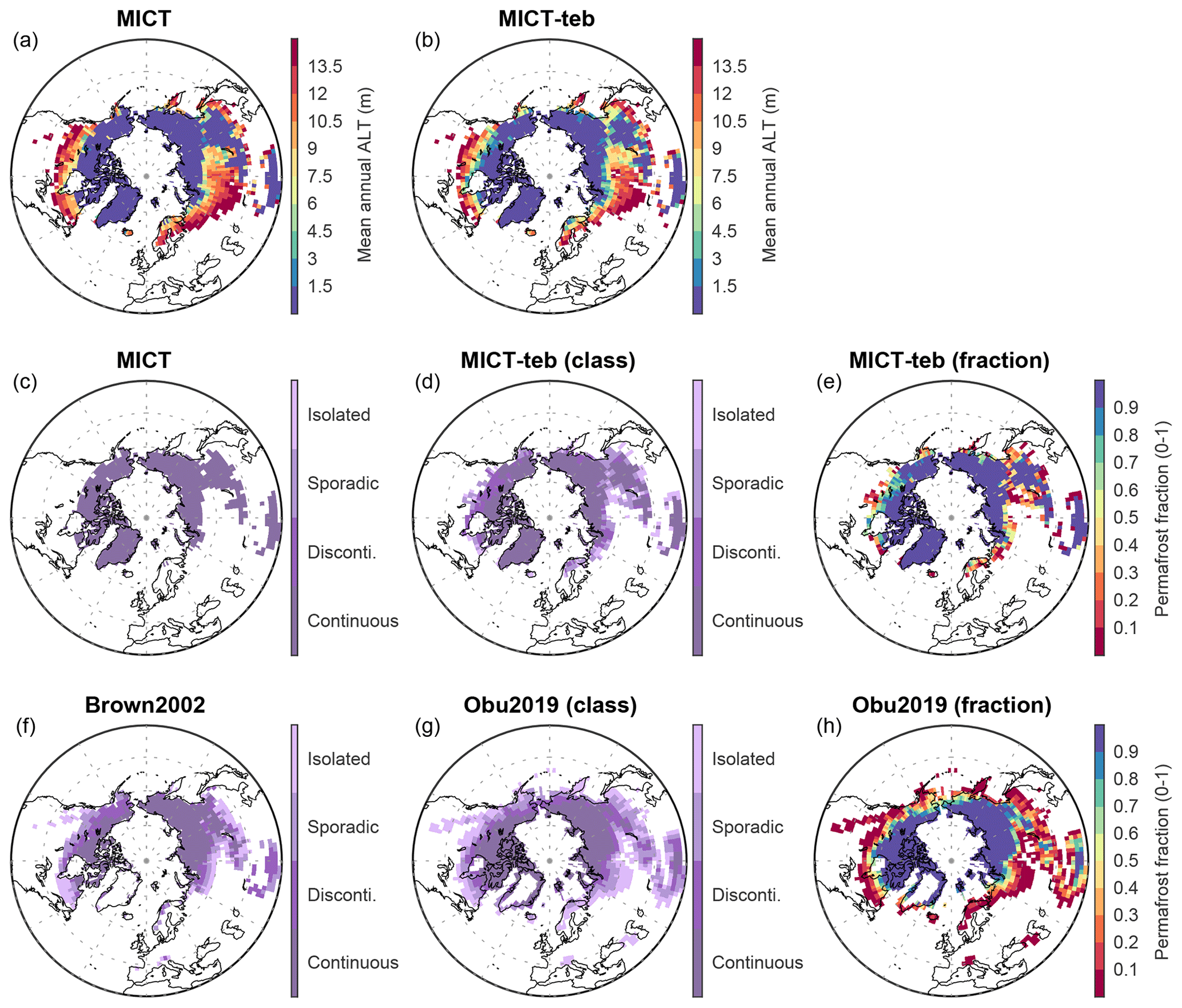
Figure 18 Evaluation of simulated permafrost areas with independent permafrost datasets. (a, b) Spatial patterns of the active layer thickness (ALT) simulated by MICT and MICT-teb. (c, e) Spatial patterns of permafrost areas simulated by MICT and MICT-teb according to the definition of ALT. (f–h) Spatial patterns of permafrost areas from Brown2002 and Obu2019. The permafrost areas in panels (c), (d), (f), and (g) are shown following four permafrost classes from Brown2002, while the permafrost areas in panels (e) and (h) are shown as the absolute fraction.

For the simulated soil energy budget, we evaluate the T_soil at 20 cm with in situ observations from across 268 Russian meteorological station sites (Sherstiukov, 2012). The period of the site data spans from 1980 to 2000. To avoid the bias resulting from missing values, we exclude 69 sites containing missing values for a specific month in over half of years. As shown in Figs. 17 and S19, the simulated mean annual T_soil at 20 cm from MICT and MICT-teb can well reproduce the spatial gradient of observed values, with a strong and positive correlation (R = 0.94; p < 0.001). However, when it comes to the mean seasonal cycle of T_soil, a warmer T_soil during winter and a cooler T_soil during summer are simulated in comparison with observations, especially for sites located in continuous permafrost regions (Fig. 17c). Apart from climate forcing data uncertainties, as suggested by Guimberteau et al. (2018), SM, SOC, and snow cover are three factors most likely to regulate the seasonal amplitude of T_soil. Guimberteau et al. (2018) have demonstrated that snow insulation is underestimated by MICT when using either the GSWP3 dataset or the CRUNCEP dataset to force the model. This implies that, from a snow perspective, our simulation should exhibit an amplified seasonal cycle. Conversely, the simulated dampened seasonal amplitude of T_soil indicates the potentially crucial roles of SM and SOC. Due to the inclusion of the peat PFT in our simulations and the use of simulated SOC rather than prescribed SOC maps to regulate soil thermal properties, the uncertainties in prescribed peatland maps and simulated SOC could propagate the uncertainties in T_soil. Moreover, we extract LST in the year 2000 across these sites from MODIS data and find a weak correlation between the bias in T_surf against MODIS and the bias in T_soil against site data (R = 0.19, p < 0.01 for all sites; R = −0.01, p > 0.05 for continuous permafrost sites; R = 0.03, p > 0.05 for other sites), suggesting potential uncertainties in observed data from different sources.

As for the impacts of tiling energy budgets on T_surf, our simulations suggest that the variation in albedo plays a dominant role at high latitudes, whereas the variation in H_rough is more significant at low latitudes (Table 2). This result is consistent with numerous studies on the biophysical feedbacks of land cover change, as the use of PFT-specific H_rough and albedo for tree PFTs can be seen as an analogy to reforestation or afforestation, while the use of PFT-specific H_rough and albedo for grass PFTs parallels the case of deforestation or forest degradation. Flux tower measurements, satellites, and climate models have revealed that tropical tree planting mitigates warming through evaporative cooling, while the low albedo of new boreal forests is a positive climate forcing (Betts, 2000; Bonan, 2008; Peng et al., 2014; Su et al., 2023). In contrast, the conversion of forests to grasslands or forest degradation shows a warming effect in tropical regions but a cooling effect in boreal regions (Lawrence and Vandecar, 2015; Alkama and Cescatti, 2016; Li et al., 2022; Zhu et al., 2023). This consistency confirms the modifications that we made in the new MICT version.

6.2 Improvements for permafrost simulations

Given the crucial role of T_soil in permafrost simulations, we compare the simulated permafrost extent from MICT and MICT-teb with two independent permafrost datasets from Brown et al. (2002) and Obu et al. (2019), hereafter referred to as Brown2002 and Obu2019, respectively (Fig. 18). Brown's map is compiled based on national and regional maps as well as empirical knowledge, categorizing permafrost into four classes: continuous permafrost (permafrost fraction > 0.9), discontinuous permafrost (0.5–0.9), sporadic permafrost (0.1–0.5), and isolated patches (0–0.1) (Brown et al., 2002). Obu's map is generated using a temperature model to simulate soil thermal regimes in three dimensions at a 300 m × 300 m spatial resolution (Obu et al., 2019). The Obu2019 data provide the absolute fraction of the landscape affected by permafrost when aggregated to a coarser grid cell (Obu et al., 2019). The simulated permafrost areas are identified following two definitions given by Guimberteau et al. (2018): (1) an active layer thickness (ALT) less than 3 m or (2) the T_soil of any soil layer remains below 0 °C for at least 2 years. As the simulated permafrost areas are very similar between the two definitions, we only show the results using the ALT definition in the paper; the results using the T_soil definition are given in the Supplement (Fig. S20 in the Supplement).

Overall, our models can capture the spatial pattern of continuous permafrost from the two independent datasets. However, the simulated total area of continuous permafrost from MICT after excluding Greenland (18.5 ×10⁶ km²) is 7.6 ×10⁶ and 6.9 ×10⁶ km² larger than that from Brown2002 and Obu2019, respectively, primarily due to the overestimation of continuous permafrost in the middle to high latitudes of Asia and the Tibetan Plateau. Given that the grid cell mean T_soil in MICT-teb is ∼ 0.5 °C warmer over the NH compared with MICT (Fig. 8), the total area of continuous permafrost simulated by MICT-teb (15.2 ×10⁶ km²) decreases by 3.3 ×10⁶ km² compared with that in MICT. Limited by the grid-cell-averaged energy budgets, MICT cannot simulate noncontinuous permafrost (i.e., a grid cell in MICT is either 100 % permafrost or 100 % non-permafrost), whereas the separation of PFT-specific T_soil in MICT-teb allows the existence of noncontinuous permafrost (Fig. 18e). The sum of all four permafrost areas (including three discontinuous classes) in MICT-teb is 18.3 ×10⁶ km² (continuous, 15.2 ×10⁶ km²; noncontinuous, 3.1 ×10⁶ km²), which is comparable to 16.9 ×10⁶ km² in Obu2019 (continuous, 11.6 ×10⁶ km²; noncontinuous, 5.3 ×10⁶ km²).

6.3 Remarks on the tiling land surface scheme

The tiling work in this study was initiated because of the planned introduction of new arctic landforms for permafrost regions into ORCHIDEE-MICT that require independent energy budgets and carbon and water cycles. The decision to tile by PFT, rather than by other units, was determined based on the current model structure. In the new version, additional variables with a new PFT dimension were introduced only for the energy module, rather than all modules, resulting in a 15 %–20 % slower run time compared with the initial version. Recently, several other model groups have also been working on tiling and the evaluation of its impacts on existing and new processes, such as JULES (Rumbold et al., 2023) and CLASSIC (Melton et al., 2017). The implementation of tiling in different land surface models can be compared to inspire other groups planning to represent the sub-grid heterogeneity of energy budgets in their models. Moreover, it is worth reminding potential users of our new version to carefully consider when and where to apply tiling in their studies in order to optimize research objectives and computational costs.

7 Conclusion

This study describes the new representation of tiling energy budgets in the ORCHIDEE-MICT land surface model and investigates its short-term and long-term impacts on energy, hydrology, and carbon processes. Instead of using grid cell mean surface properties, like roughness height and albedo, PFT-specific values are employed for each vegetation type, and all of the associated energy, hydrology, and carbon processes are modified in the model. Compared with the original version, the separation of PFT-specific energy budgets results in warmer surface and soil temperatures, higher soil moisture, and increased soil organic carbon storage across the Northern Hemisphere. Evaluation with satellite products and site measurements suggests that the new version can reproduce the spatial distributions and seasonal patterns of surface and soil temperature. However, notable positive or negative biases are observed in some regions due to remaining weaknesses in the original ORCHIDEE-MICT model, such as the uncertainties involved in simulating soil moisture and soil organic carbon, as well as uncertainties in the prescribed peatland map. A notable advancement in the new version is the improved simulation of permafrost extent by accounting for the presence of discontinuous permafrost, which will facilitate various permafrost-related studies based on the model in the future.