the Creative Commons Attribution 4.0 License.
the Creative Commons Attribution 4.0 License.
 | 22 May 2024
Parallel SnowModel (v1.0): a parallel implementation of a distributed snow-evolution modeling system (SnowModel)
Ross Mower
Ethan D. Gutmann
Glen E. Liston
Jessica Lundquist
Soren Rasmussen
SnowModel, a spatially distributed snow-evolution modeling system, was parallelized using Coarray Fortran for high-performance computing architectures to allow high-resolution (1 m to hundreds of meters) simulations over large regional- to continental-scale domains. In the parallel algorithm, the model domain was split into smaller rectangular sub-domains that are distributed over multiple processor cores using one-dimensional decomposition. All the memory allocations from the original code were reduced to the size of the local sub-domains, allowing each core to perform fewer computations and requiring less memory for each process. Most of the subroutines in SnowModel were simple to parallelize; however, there were certain physical processes, including blowing snow redistribution and components within the solar radiation and wind models, that required non-trivial parallelization using halo-exchange patterns. To validate the parallel algorithm and assess parallel scaling characteristics, high-resolution (100 m grid) simulations were performed over several western United States domains and over the contiguous United States (CONUS) for a year. The CONUS scaling experiment had approximately 70 % parallel efficiency; runtime decreased by a factor of 1.9 running on 1800 cores relative to 648 cores (the minimum number of cores that could be used to run such a large domain because of memory and time limitations). CONUS 100 m simulations were performed for 21 years (2000–2021) using 46 238 and 28 260 grid cells in the x and y dimensions, respectively. Each year was simulated using 1800 cores and took approximately 5 h to run.
- Article
(4899 KB) - Full-text XML
- BibTeX
- EndNote


The cryosphere (snow and ice) is an essential component of Arctic, mountain, and downstream ecosystems, Earth's surface energy balance, and freshwater resource storage (Huss et al., 2017). Globally, half the world's population depends on snowmelt (Beniston, 2003). In snow-dominated regions like the western United States, snowmelt contributes to approximately 70 % of the total annual water supply (Foster et al., 2011). In these regions, late-season streamflow is dependent on the deepest snowdrifts and therefore longest-lasting snow (Pflug and Lundquist, 2020). Since modeling snow-fed streamflow accurately is largely dependent on our ability to predict snow quantities and the associated spatial and temporal variability (Clark and Hay, 2004), high-temporal- and spatial-resolution snow datasets are important for predicting flood hazards and managing freshwater resources (Immerzeel et al., 2020).
The spatial and temporal seasonal snow characteristics also have significant implications outside of water resources. Changes in fractional snow-covered area affect albedo and thus atmospheric dynamics (Liston, 2004; Liston and Hall, 1995). Avalanches pose safety hazards to both transportation and recreational activities in mountainous terrain, the prediction of which requires high-resolution (meters) snow datasets (Morin et al., 2020; Richter et al., 2021). Additionally, the timing and duration of snow-covered landscapes strongly influence how species adapt, migrate, and survive (Boelman et al., 2019; Liston et al., 2016; Mahoney et al., 2018).
To date, the primary modes for estimating snow properties and storage have come from observation networks, satellite-based sensors, and physically derived snow algorithms in land surface models (LSMs). However, despite the importance of regional, continental, and global snow, estimates of snow properties over these scales remain uncertain, especially in alpine regions where wind, snow, and topography interact (Boelman et al., 2019; Dozier et al., 2016; Mudryk et al., 2015). Observation datasets used for spatial interpolation of snow properties and forcing datasets used in LSMs are often too sparse in mountainous terrain to accurately resolve snow spatial heterogeneities (Dozier et al., 2016; Renwick, 2014). Additionally, remotely sensed products have shown deficiencies in measuring snowfall rate (Skofronick-Jackson et al., 2013), snow-water equivalent (SWE), and snow depth (Nolin, 2010), especially in mountainous terrain where conditions of deep snow, wet snow, and/or dense vegetation may be present (Lettenmaier et al., 2015; Takala et al., 2011; Vuyovich et al., 2014). However, LSMs using high-resolution inputs, including forcing datasets from regional climate models (RCMs), have demonstrated realistic spatial distributions of snow properties (Wrzesien et al., 2018).
Many physical snow models have been developed either in stand-alone algorithms or larger LSMs with varying degrees of complexity based on their application. The more advanced algorithms attempt to accurately model snow properties at high resolution, especially in regions where snow interacts with topography, vegetation, and/or wind. Wind-induced snow transport is one such complexity of snow that represents an important interaction between the cryosphere and atmosphere. It occurs in regions permanently or temporarily covered by snow, influences snow properties (e.g., heterogeneity, sublimation, avalanches, and melt timing), and has been shown to improve simulated snowpack distribution (Bernhardt et al., 2012; Freudiger et al., 2017; Keenan et al., 2023; Quéno et al., 2023). Models that have incorporated wind-induced physics generally require components to both develop the snow mass balance and incorporate atmospheric inputs of the wind field. Additionally, these models typically require high-resolution grids (1 to 100 m) as the redistribution components of the model become negligible at larger spatial discretizations (Liston et al., 2007). However, there is often a trade-off between the accuracy of simulating wind-induced snow transport and the computational requirements for downscaling and developing the wind fields over the gridded domain (Reynolds et al., 2021; Vionnet et al., 2014). Therefore, simplifying assumptions of uniform wind direction has been applied in models like the Distributed Blowing Snow Model (DBSM) (Essery et al., 1999; Fang and Pomeroy, 2009). More advanced models have utilized advection–diffusion equations, like Alpine3D (Lehning et al., 2006), or spatial distributed formulations like SnowTran-3D (Liston and Sturm, 1998). Finite-volume methods for more efficiently discretizing wind fields have been applied to models such as DBSM (Marsh et al., 2020). The most complex models consider nonsteady turbulence and utilize three-dimensional wind fields from atmospheric models to simulate blowing snow transport and sublimation: for example, SURFEX in Meso-NH/Crocus (Vionnet et al., 2014, 2017), wind fields from the atmospheric model ARPS (Xue et al., 2000) being incorporated into Alpine3D (Mott and Lehning, 2010; Mott et al., 2010; Lehning et al., 2008), and SnowDrift3D (Prokop and Schneiderbauer, 2011). Incorporating wind-induced physics into snow models is computationally expensive; thus, parallelizing the serial algorithms would likely be beneficial to many models.
For several decades, a distributed snow-evolution modeling system (SnowModel) has been developed, enhanced, and tested to accurately simulate snow properties across a wide range of landscapes, climates, and conditions (Liston and Elder, 2006a; Liston et al., 2020). To date, SnowModel has been used in over 200 refereed journal publications; a short listing of these is provided by Liston et al. (2020). Physically derived snow algorithms, as used in SnowModel, that model the energy balance, multi-layer snow physics, and lateral snow transport are computationally expensive. In these models, the required computational power increases with the number of grid cells covering the simulation domain. Finer grid resolutions usually imply more grid cells and higher accuracy resulting from improved representation of process physics at higher resolutions. The original serial SnowModel code was written in Fortran 77 and could not be executed in parallel using multiple processor cores. As a result, SnowModel's spatial and temporal simulation domains (number of grid cells and time steps) were previously limited by the speed of one core and the memory available on the single computer. Note that a “processor” refers to a single central processing unit (CPU) and typically consists of multiple cores; each core can run one or more processes in parallel.
Recent advancements in multiprocessor computer technologies and architectures have allowed for increased performance in simulating complex natural systems at high resolutions. Parallel computing has been used on many LSMs to reduce computing time and allow for higher-accuracy results from finer grid simulations (Hamman et al., 2018; Miller et al., 2014). Our goal was to develop a parallel version of SnowModel (Parallel SnowModel) using Coarray Fortran (CAF) syntax without making significant changes to the original SnowModel code physics or structure. CAF is a partitioned global address space (PGAS) programming model and has been used to run atmospheric models on 100 000 cores (Rouson et al., 2017).
In parallelizing numerical models, a common strategy is to decompose the domain into smaller sub-domains that get distributed across multiple processes (Dennis, 2007; Hamman et al., 2018). For rectangular gridded domains (like SnowModel), this preserves the original structure of the spatial loops and utilizes direct referencing of neighboring grids (Perezhogin et al., 2021). The parallelization of many LSMs involves “embarrassingly parallel” problems requiring minimal to no processor communication (Parhami, 1995); in this case, adjacent grid cells do not communicate with each other (an example of this would be where each grid cell represents a point, or one-dimensional, snowpack model that is not influenced by nearby grid cells).
While much of the SnowModel's logic can be considered embarrassingly parallel, SnowModel also contains “non-trivial” algorithms within the solar radiation, wind, and snow redistribution models. Calculations within these algorithms often require information from neighboring grid cells, either for spatial derivative calculations or for horizontal fluxes of mass (e.g., saltating or turbulent suspended snow) across the domain. Therefore, non-trivial parallelization requires implementing algorithm changes that allow computer processes to communicate and exchange data. The novelty of the work presented here includes (1) the presentation of Parallel SnowModel, high-resolution (100 m) distributed snow datasets over CONUS, and an analysis of the performance of the parallel algorithm; (2) demonstrating how a simplified parallelization approach using CAF and one-dimensional decomposition can be implemented in geoscientific algorithms to scale over large domains; and (3) demonstrating an approach for non-trivial parallelization algorithms that involve spatial derivatives and fluxes using halo-exchange techniques.
In Sect. 2, we provide background information on SnowModel, parallelization using CAF, data and domains used in this study, and a motivation for this work. In Sect. 3, we explain our parallelization approach using CAF and introduce the simulation experiments used to demonstrate the performance of Parallel SnowModel through strong scaling metrics and CONUS simulations. In Sect. 4, we provide results of the simulation experiments introduced in Sect. 3. Lastly, we end with a discussion in Sect. 5 and a conclusion in Sect. 6.
2.1 SnowModel
SnowModel is a spatially distributed snow-evolution modeling system designed to model snow states (e.g., snow depth, SWE, snowmelt, snow density) and fluxes over different landscapes and climates (Liston and Elder, 2006a). The most complete and up-to-date description of SnowModel can be found in the appendices of Liston et al. (2020). While many snow modeling systems exist, SnowModel will benefit from parallelization because of its ability to simulate snow processes on a high-resolution grid through downscaling meteorological inputs and modeling snow redistribution. SnowModel is designed to simulate domains on a structured grid with spatial resolutions ranging from 1 to 200 m (although it can simulate coarser resolutions as well) and temporal resolutions ranging from 10 m to 1 d. The primary modeled processes include accumulation from frozen precipitation; blowing snow redistribution and sublimation; interception, unloading, and sublimation within forest canopies; snow density and grain size evolution; and snowpack ripening and melt. These processes are distributed into four core interacting submodules: MicroMet defines the meteorological forcing conditions (Liston and Elder, 2006b), EnBal describes surface and energy exchanges (Liston, 1995; Liston et al., 1999), SnowPack-ML is a multi-layer snowpack sub-model that simulates the evolution of snow properties and the moisture and energy transfers between layers (Liston and Hall, 1995; Liston and Mernild, 2012), and SnowTran-3D calculates snow redistribution by wind (Liston et al., 2007). Additional simulation features include SnowDunes (Liston et al., 2018) and SnowAssim (Liston and Hiemstra, 2008), which model sea ice applications and data assimilation techniques, respectively. Figure 1 shows a schematic of the core SnowModel toolkit. Additionally, the initialization submodules that read in the model parameters, distribute inputs across the modeled grid, and allocate arrays include PreProcess and ReadParam. Outputting arrays is contained within the “Outputs” submodule. SnowModel incorporates first-order physics required to simulate snow evolution within each of the global snow classes (e.g., ice, tundra, boreal forest, montane forest, prairie, maritime, and ephemeral; Sturm and Liston, 2021; Liston and Sturm, 2021).

Figure 1The original figure from Pedersen et al. (2015) was modified for the present paper, providing an example of possible inputs, core submodules, and outputs of SnowModel.
2.2 Coarray Fortran
CAF, formerly known as F- (Iso/Iec, 2010; Numrich and Reid, 1998; Numrich et al., 1998), is the parallel language feature of Fortran that was used to parallelize SnowModel. CAF is like Message Passing Interface (MPI) libraries in that it uses the single-program multiple-data (SPMD) model where multiple independent cores simultaneously execute a program. SPMD allows for distributed memory allocation and remote memory transfer. However, unlike MPI, CAF uses the PGAS parallel programming model to handle the distribution of computational tasks amongst processes (Coarfa et al., 2005). In the PGAS model, each process contains local memory that can be accessed directly by all other processes. While CAF and MPI syntax often refers to processes as images or ranks, for consistency, we will continue to use the term “process”. Ultimately, CAF offers a high-level syntax that exploits locality and scales effectively (Coarfa et al., 2005). For simulation comparisons, we used OpenCoarrays, a library implementation of CAF (Fanfarillo et al., 2014) utilized by the gfortran compiler; Intel and Cray compilers both have independent CAF implementations.
2.3 Model domains, data, and computing resources
The required inputs for SnowModel include (1) temporally varying meteorological variables of precipitation, wind speed and direction, air temperature, and relative humidity taken from meteorological stations or atmospheric models and (2) spatially distributed topography and land cover type (Liston and Elder, 2006a). The following inputs were used for the experiments introduced in Sect. 3: the USGS National Elevation Dataset (NED) for topography (Gesch et al., 2018), the North American Land Change Monitoring System (NALCMS) land cover 2015 map for vegetation (Homer et al., 2015; Jin et al., 2019; Latifovic et al., 2016), and forcing variables from either the North American Land Data Assimilation System (NLDAS-2) (Mitchell, 2004; Xia, 2012a, b) on a ° (approximately 12 km) grid or the high-resolution Weather Research and Forecasting (WRF) model from the National Center for Atmospheric Research (NCAR) on approximately a 4 km grid (Rasmussen et al., 2023). The high-performance computing architectures used include NCAR's Cheyenne supercomputer, which is a 5.43-petaflop SGI ICE XA cluster featuring 145 152 Intel Xeon processes in 4032 dual-socket nodes and 313 TB of total memory (Computational and Information Systems Laboratory, 2019), and the National Aeronautics and Space Administration's (NASA) Center for Climate Simulation (NCCS) Discover supercomputer with a 1560-teraflop SuperMicro Cluster featuring 20 800 Intel Xeon Skylake processes in 520 dual-socket nodes and 99.84 TB of total memory. Simulation experiments were conducted over six domains (Tuolumne, CO headwaters, Idaho, PNW, western US, and CONUS) throughout the United States at 100 m grid resolution. The spatial location, domain dimensions (e.g., number of grids in the x and y dimensions), and memory requirements, derived from the peak_memusage package (https://github.com/NCAR/peak_memusage, last access: 10 July 2023), for the simulation experiments are highlighted in Fig. 2.
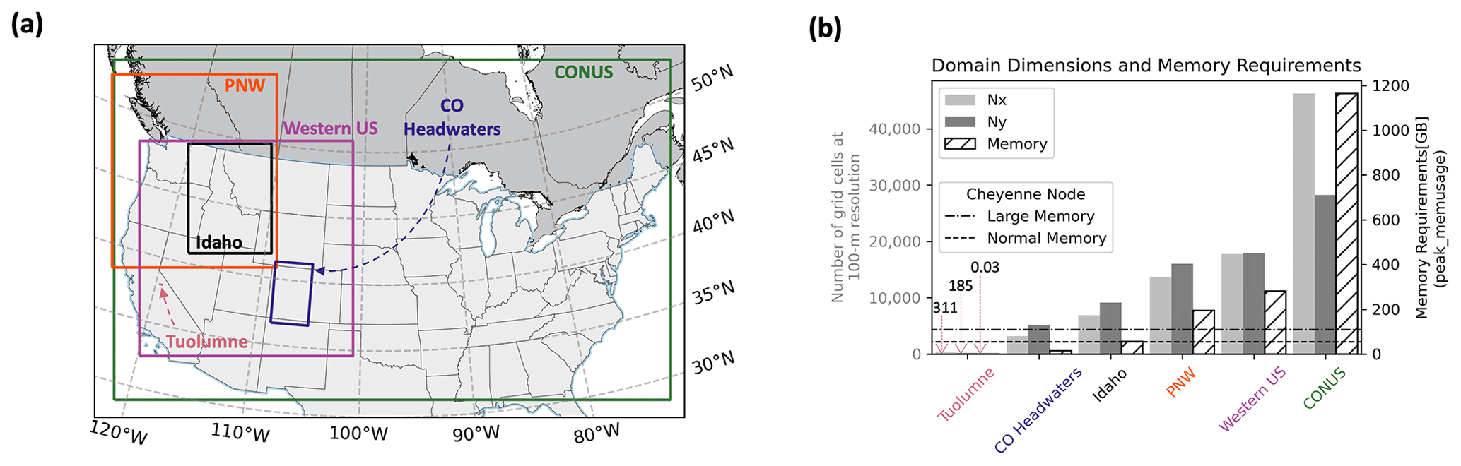
Figure 2(a) Spatial location of simulated domains on WRF's Lambert conformal projection (Rasmussen et al., 2023) and (b) corresponding grid dimensions (Nx – number of grids in x dimension; Ny – number of grids in y dimension) and memory obtained from the peak_memusage package required for single-layer SnowModel simulation experiments. For reference, the dashed lines represent the normal and large memory thresholds (55 and 109 GB) for Cheyenne's SGI ICE XA cluster.
2.4 Parallelization motivation
The answers to current snow science, remote sensing, and water management questions require high-resolution data that cover large spatial and temporal domains. While modeling systems like SnowModel can be used to help provide these datasets, running them on single-processor workstations imposes limits on the spatiotemporal extents of the produced information. Serial simulations are limited by both execution time and memory requirements, where the memory limitation is largely dependent on the size of the simulation domain. Up to the equivalent of 175 two-dimensional and 10 three-dimensional arrays are held in memory during a SnowModel simulation, depending on the model configuration. In analyzing the performance of the Parallel SnowModel (Sect. 4), serial simulations were attempted over six domains throughout the United States at 100 m grid resolution (Fig. 2) for the 2018 water year (1 September 2017 to 1 September 2018). Only the Tuolumne domain could be simulated in serial based on the memory (109 GB for a large memory node) and time (12 h wall-clock limit) constraints on Cheyenne. The CO headwaters and Idaho domains could not be simulated in serial due to time constraints, while the three largest domains (Pacific Northwest – PNW, western US, and CONUS) could not be executed in serial due to exceedances of both the 12 h wall-clock limit and memory availability. Furthermore, we estimate that using a currently available, state-of-the-art, single-processor workstation would require approximately 120 d of computer time to perform a 1-year model simulation over the CONUS domain. SnowModel is regularly used to perform multi-decade simulations for trend analyses, climate change studies, and retrospective analyses (Liston and Hiemstra, 2011; Liston et al., 2020, 2023). If this 1-year, 100 m CONUS domain was simulated for a 40-year period (e.g., 1980 through the present), it would take approximately 4800 d, or over 13 years, of computer time. Clearly such simulations are not practical using single-processor computer hardware and software algorithms.
In parallelizing SnowModel and distributing computations and memory over multiple processes, we demonstrate its ability to efficiently run regional- to continental-sized simulations. Some of the model configurations were not parallelized for reasons including ongoing development in the serial code base and limitations to the parallelization approach. These configurations are further discussed in Appendix A. This section introduces the syntax and framework used to parallelize SnowModel and the simulation experiments used to assess the performance of the parallel algorithm.
3.1 Parallel implementation
Changes to the SnowModel logic were made through the parallelization process and included the partitioning algorithm, non-trivial communication via halo exchange, and file input and output (I/O) schemes.
3.1.1 Partitioning algorithm
The partitioning strategy identifies how the workload gets distributed amongst processes in a parallel algorithm. The multidimensional arrays of SnowModel are stored in row-major order, meaning the x dimension is contiguous in memory. Additionally, dominant wind directions and therefore predominant snow redistribution occur in the east–west direction as opposed to south–north directions. Therefore, both the data structures and physical processes involved in SnowModel justify a one-dimensional decomposition strategy in the y dimension, where the computational global domain Nx×Ny is separated into Nx×lny blocks. If Ny is evenly divisible by the total number of processes (N), . If integer division is not possible, the remaining rows are distributed evenly amongst the processes starting at the bottom of the computational domain. Figure 3 demonstrates how a serial domain containing 10 grid cells in the x and y dimensions would be decomposed with four processes using our partitioning strategy.
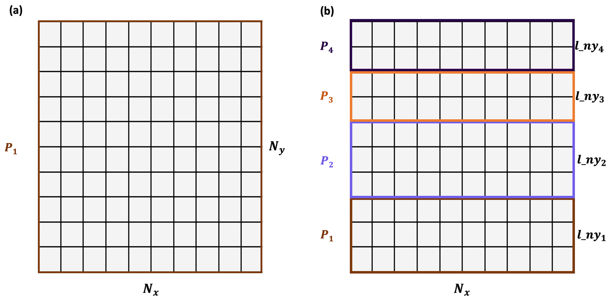
Figure 3Example 10×10 global domain and partitioning for (a) serial simulation and (b) parallel simulation using four processes.
3.1.2 Non-trivial parallelization
Each process has sufficient information to correctly execute most of the physical computations within SnowModel. However, there are certain subroutines where grid computations require information from neighboring grid cells (e.g., data dependencies) and therefore information outside of the local domain of a process. For SnowModel, these subroutines typically involve the transfer of blowing snow or calculations requiring spatial derivatives. Furthermore, with our one-dimensional decomposition approach, each grid cell within a process local domain has sufficient information from its neighboring grid cells in the x dimension but potentially lacks information from neighboring grid cells in the y dimension. As a regular grid method, SnowModel lends itself to process communication via halo exchange where coarrays are used in remote calls. Halo exchange using CAF involves copying boundary data into coarrays on neighboring processes and using information from the coarrays to complete computations (Fig. 4). Although the entire local array could be declared a coarray and accessed by remote processes more directly, some CAF implementations (e.g., Cray) impose additional constraints upon coarray memory allocations that can be problematic for such large allocations.
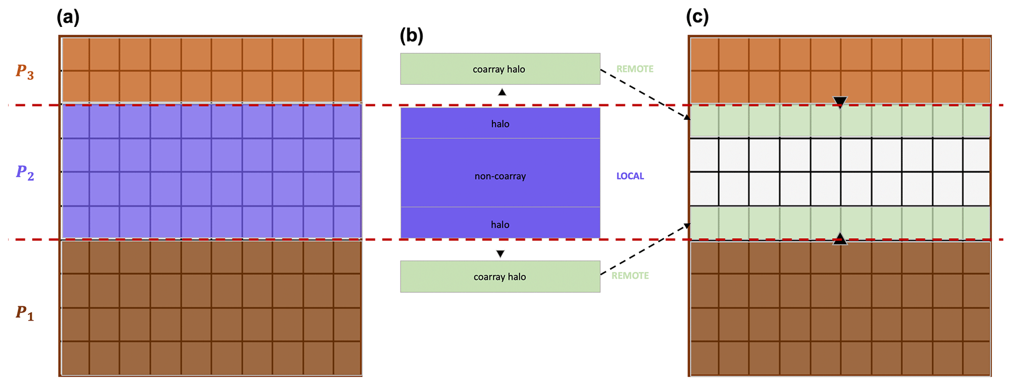
Figure 4Schematic showing halo exchange using coarrays. The steps include (a) initial gridded representation of local arrays for three processes, (b) P2 copying boundary data into coarrays for remote access, and (c) neighboring processes (P1 and P3) stitching coarray to local domains.
Topography – wind and solar radiation models
The wind and solar radiation models in MicroMet require information about surrounding surface topography (Liston and Elder, 2006b). The wind model requires surface curvature, and the solar radiation model requires surface slope and aspect. These vary at each time step as snow accumulates and melts because the defined surface includes the snow surface on top of the landscape. The surface curvature, for example, is computed at each model grid cell using the spatial gradient of the topographic elevation of eight neighboring grid cells. Using the parallelization approach discussed above, processes lack sufficient information to make curvature calculations for the bordering grid cells along the top and/or bottom row(s) within their local domains. Note that the number of row(s) (inc) is determined by a predefined parameter that represents the wavelength of topographic features within a domain. Future work should permit this parameter to vary spatially to account for changes in the length scale across the domain. For example, all grid cells along the top row of P1 will be missing information from nearby grid cells to the north and require topographic elevation (topo) information from the bottom row(s) of the local domain of P2 to make the calculation (Fig. 5a). Halo exchange is performed to distribute row(s) of data to each process that is missing that information in their local domains (Fig. 5b). Processes whose local domains are positioned in the bottom or top of the global domain will only perform one halo exchange with their interior neighbor, while interior processes will perform two halo exchanges. By combining and appropriately indexing information from the process local array and received coarrays of topographic elevation, an accurate curvature calculation can be performed using this parallel approach (Fig. 5c).
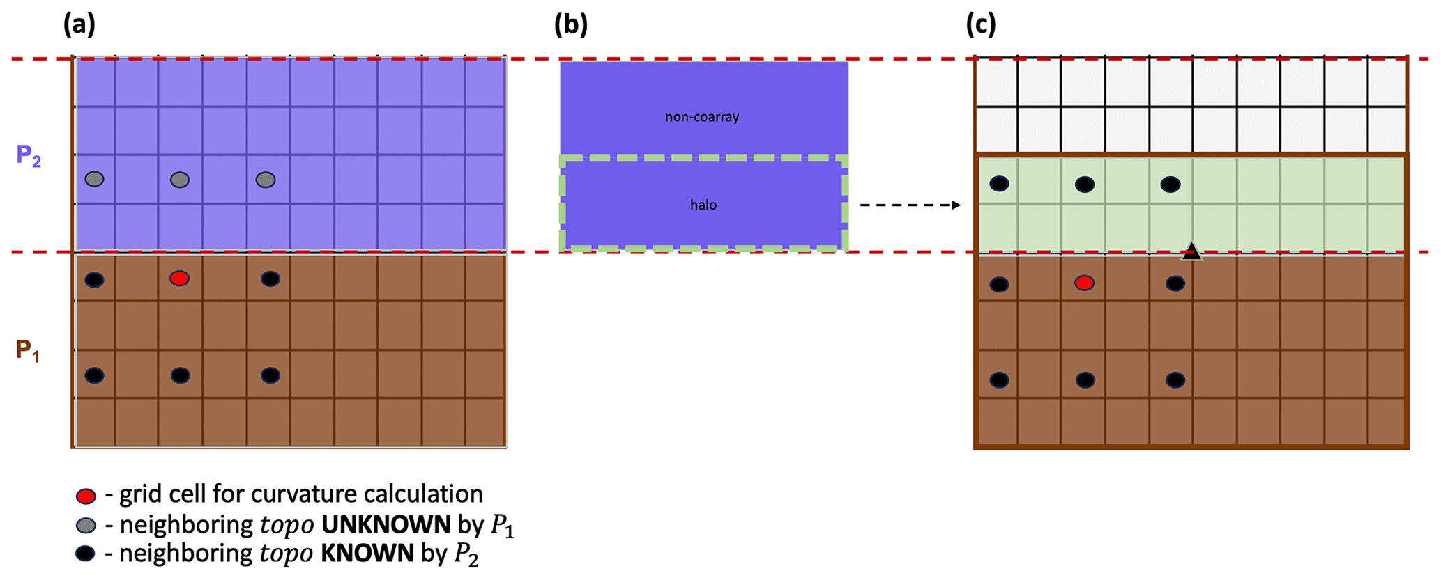
Figure 5Schematic for halo exchange used in the curvature calculation by P1, where inc = 2. (a) Prior to halo exchange, P1 contains insufficient information to perform the curvature calculation, and (b) grid cells (halo) within the local domain of P2 are (c) transferred to P1 via coarrays. At this point, P1 has sufficient information to make the curvature calculation.
Snow redistribution
Wind influences the mass balance of the snowpack by suspending and transporting snow particles in the air (turbulent suspension) and by causing snow grains to bounce on top of the snow surface (saltation). In SnowModel, the saltation and suspension algorithms are separated into northerly, southerly, easterly, and westerly fluxes based on the u and v components of wind direction for each grid cell. Figure 6 shows a simplified schematic for the saltation flux from a southerly wind. In the serial algorithm (Fig. 6a), SnowModel initializes the saltation flux based on the wind speed at that time step (initial flux). To calculate the final saltation flux (updated flux), SnowModel steps through regions of continuous wind direction (delineated by the indices jstart and jend), updates the change in saltation fluxes from upwind grid cells and the change in saltation flux from the given wind direction, and makes adjustments to these fluxes based on the soft snow availability above the vegetation height (Liston and Elder, 2006a). Similar logic is used for the parallel implementation of the saltation and suspension fluxes with an additional iteration (salt iter) that updates the boundary condition for each process via halo exchange. This allows the fluxes to be communicated from the local domain of one process to another. To minimize the number of iterations, salt iter was provided a maximum bound that is equivalent to snow being transported 15 km via saltation or suspension. This number was chosen based on prior field measurements (Tabler, 1975) and simulation experiments. It is possible that in other environments an even larger length may be required. To be guaranteed to match the serial results in all cases, the number of iterations would have to be equal to the number of processes; however, this would result in no parallel speedup and has no practical benefit. A schematic of the parallel calculation of the change in saltation due to southerly winds is illustrated in Fig. 6b. The bc_halo_exchange represents a halo exchange of grid cells from upwind processes, allowing the saltation flux to be transported from one process local domain to the next.
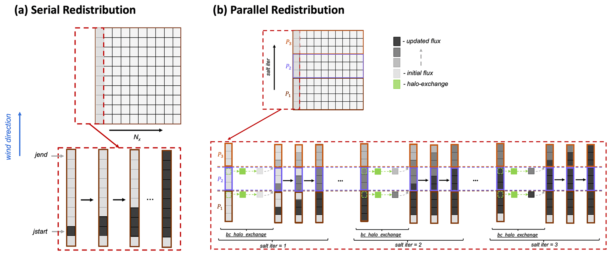
Figure 6(a) Schematic of the serial and (b) parallel redistribution algorithm showing the change in saltation flux due to southerly winds over a gridded domain for Nx=1. The parallel schematic demonstrates how three processes (P1, P2, P3) use an additional iteration (salt iter) to perform a halo exchange (bc_halo_exchange) and update the boundary condition of the saltation flux.
3.1.3 File I/O
File I/O management can be a significant bottleneck in parallel applications. Parallel implementations that are less memory-restricted commonly use local to global mapping strategies, or a centralized approach for file I/O (Fig. 7a). This approach requires that one or more processes stores global arrays for input variables and that one process (Process 1; Fig. 7a) stores global arrays for all output variables. As the domain size increases, the mapping of local variables to global variables for outputting creates a substantial bottleneck. To improve performance, distributed file I/O can be implemented, where input and output files are directly and concurrently accessed by each process (Fig. 7b).
SnowModel contains static spatial inputs that do not vary over time (e.g., topography and land cover) and dynamic spatial inputs (e.g., air temperature and precipitation) that vary spatially and temporally. The static inputs are of a higher resolution compared to the dynamic inputs (i.e., topography is on the model grid, while atmospheric forcing is almost always more widely spaced). To balance performance and consistency with the serial logic of the code, we used a mixed parallel file I/O approach. A goal of this work was to maintain nearly identical serial and parallel versions of the code in one code base that can be easily maintained and utilized by previous, current, and future SnowModel users with different computational resources and skills. Therefore, we wanted to maintain both the centralized and distributed file I/O approaches. However, for optimal parallel performance over larger simulation domains, file input (reading) is performed in a distributed way for the static inputs and in a centralized way for dynamic inputs, while file output (writing) is performed in a distributed way, as described further below. This permits the new version of the code to be a drop-in replacement for the original serial code without requiring users to install new software libraries or manage hundreds of output files, while enabling users who wish to take advantage of the parallel nature of the code to do so with minimal additional work and no changes to the underlying code.
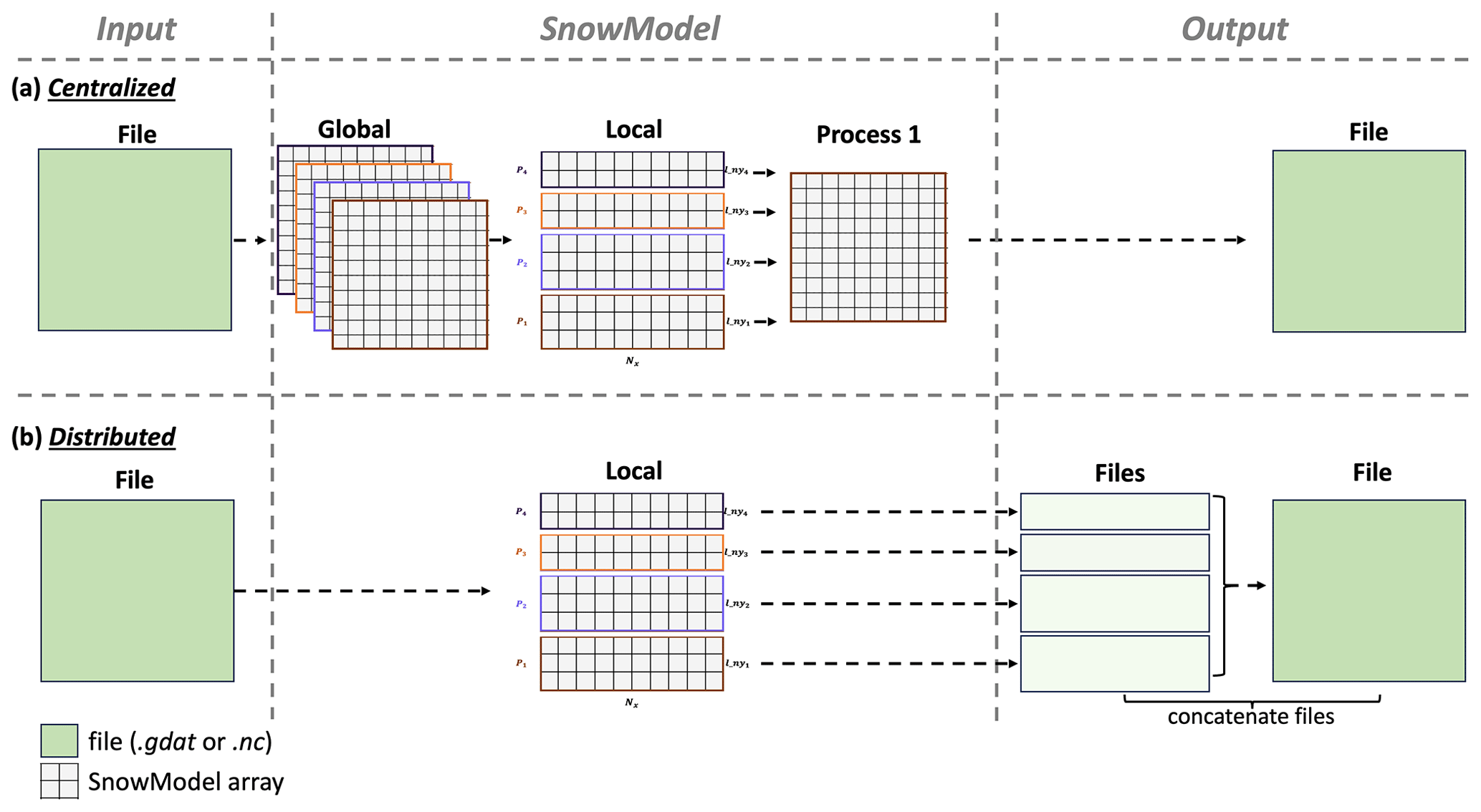
Figure 7(a) Schematic of global to local mapping for file I/O using a centralized approach with four processes and a (b) distributed file I/O where each process reads and writes data corresponding to its local domain.
Parallel inputs
As noted above, SnowModel has two primary types of input files, temporally static files such as vegetation and topography and transient inputs such as meteorological forcing data. While acceptable static input file types include flat binary, NetCDF, and ASCII files for the serial version of the code, optimizing the efficiency of Parallel SnowModel requires static inputs from binary files that can be accessed concurrently and directly subset by indexing the starting byte and length of bytes commensurate with a process local domain. Therefore, each process can read its own portion of the static input data. For very large domains, the available memory becomes a limitation when using the centralized approach. For example, the CONUS simulation could not be simulated using a centralized file I/O approach because each process would be holding global arrays of topography and vegetation in memory, each of which would require approximately 5.2 GB of memory per process.
Reading of meteorological forcing variables (wind speed, wind direction, relative humidity, temperature, and precipitation) can be performed in parallel with either binary or NetCDF files. Depending on the forcing dataset, the grid spacing of the meteorological variables typically ranges from 1 to 30 km and therefore often requires a smaller memory footprint than static inputs for high-resolution simulations. For example, the resolution of NLDAS-2 meteorological forcing has a grid of approximately 11 km, while the high-resolution WRF model used has a 4 km grid. At each time step, processes read in the forcing data from every station within the domain into a one-dimensional array, index the nearest locations for each SnowModel grid, and interpolate the data to create forcing variables over the local domain. All processes perform the same operation and store common information; however, since the resolutions of the forcing datasets are significantly coarser than the model grid for high-resolution simulations, the dynamic forcing input array size remains comparable to other local arrays and does not impose significant memory limitations for simulations performed to date. While more efficient parallel file input schemes could improve performance, we decided to keep this logic in part to maintain consistency with the serial version of the code and minimize code changes.
Parallel outputs
To eliminate the use of local to global mapping commonly used to output variables (Fig. 7a), each process writes its own output file (Fig. 7b). A postprocessing script is then used to concatenate files from each process into one file that represents the output for the global domain. Modern high-performance computing architectures have highly parallelized storage systems, making file output using a distributed approach significantly faster than the centralized approach. Therefore, file output in this manner reduces time and memory requirements. Future work could leverage other established parallel I/O libraries at the cost of additional installation requirements.
3.2 Simulation experiments
Parallel SnowModel experiments were conducted to evaluate the effectiveness of the parallelization approach used in this study (Sect. 3.1) and to produce a high-resolution snow dataset over CONUS. All experiments were executed with a 100 m grid increment, a 3 h time step, and a single-layer snowpack configuration and included the primary SnowModel modules (MicroMet, EnBal, SnowPack, and SnowTran-3D). These experiments are further described below, with results provided in Sect. 4.
Validation experiments comparing output from the original serial version of the code to the parallel version were conducted continuously throughout the parallel algorithm development to assess the reproducibility of the results. Additionally, a more thorough validation effort was performed at the end of the study that compared output from the serial algorithm to that of the parallel algorithm, while varying the domain size, the number of processes, and therefore the domain decomposition. Results from all of these validation experiments produced root mean squared error (RMSE) values of 10−6, which is at the limit of machine precision when compared to serial simulation results. See Appendix B for more details on the validation experiments. The serial version of SnowModel has been evaluated in many studies across different snow classes (Sturm and Liston, 2021; Liston and Sturm, 2021), time periods, and snow properties. Evaluations ranged from snow cover (Pedersen et al., 2016; Randin et al., 2015) and snow depth (Szczypta et al., 2013; Wagner et al., 2023) to SWE (Freudiger et al., 2017; Hammond et al., 2023; Mortezapour et al., 2020; Voordendag et al., 2021) and SWE melt (Hoppinen et al., 2024; Lund et al., 2022) using field observations, snow-telemetry stations, and remote sensing products. A full comparison of the Parallel SnowModel simulations presented here with observations across CONUS is beyond the scope of the present work. Incorrectly simulated SWE could affect the scaling results and CONUS visualizations presented in Sect. 4; for example, if zero SWE were incorrectly simulated in many locations, processing time would be less than if SWE had been simulated and tracked. However, based on the scale of these analyses and the fact that SnowModel has been previously evaluated in a wide range of locations, we believe the impacts of this limitation on the computational results presented here are minimal.
3.2.1 Parallel performance
In high-performance computing, scalability attempts to assess the effectiveness of running a parallel algorithm with an increasing number of processes. Thus, scalability can be used to identify the optimal number of processes for a fixed domain, understand the limitations of a parallel algorithm as a function of domain size and number of processes, and estimate the efficiency of the parallel algorithm on new domains or computing architectures. Speedup, efficiency, and code profiling were tools used to assess the scalability and performance of Parallel SnowModel on fixed domains. Speedup (S(N); Eq. 1), a metric of strong scaling, is defined as the ratio of the serial execution time, T(1), over the execution time using N processes, T(N). Optimally, parallel algorithms will experience a doubling of speedup as the number of processes is doubled. Some reasons why parallel algorithms do not follow ideal scaling include the degree of concurrency possible and overhead costs due to communication. Synchronization statements have an associated cost of decreasing the speed and efficiency of an algorithm due to communication overhead and requirements for one process to sit idle while waiting for another to reach the synchronization point. Furthermore, speedup tends to peak or plateau at a certain limit on a given computing architecture and domain because either the overheads grow with an increasing number of processes or the number of processes exceeds the degree of concurrency inherent in the algorithm (Kumar and Gupta, 1991). For large domains, where serial simulations cannot be performed either due to wall-clock or memory limitations, relative speedup (; Eq. 2) is commonly used. Relative speedup is estimated as a ratio of the execution time, , of the minimum number of processes, (), that can be simulated on a given domain over T(N). An additional speedup metric, approximate speedup (; Eq. 3), is introduced to estimate S by assuming perfect scaling from to a single process. While this is only an approximation, it is helpful to compare the across the different domains on a similar scale. Additionally, efficiency (E(N); Eq. 4) and approximate efficiency (; Eq. 5) are the ratios of S to N and to N, respectively. A simulation that demonstrates ideal scaling would have 100 % efficiency. Additionally, code profiling evaluates the cumulative execution time of individual submodules (e.g., Preprocess, Readparam, MicroMet, Enbal, SnowPack, SnowTran-3D, and Outputs) as a function of the number of processes. Together, code profiling and strong scaling can be used to understand locations of bottlenecks in the algorithm and how changes to the code enhance performance.
3.2.2 Parallel improvement
To better understand how changes to the Parallel SnowModel code have affected its performance, speedup and code profiling plots were assessed for simulations using three distinct versions of the code. These versions represent snapshots of the algorithms development and quantify the contributions of different types of code modifications to the final performance of the model. These versions were identified by different GitHub commits (Mower et al., 2023) and can be summarized as follows. The first or baseline version represents an early commit of Parallel SnowModel, where file I/O is performed in a centralized way, as described in Sect. 3.1.3. Each process stores both a local and global array in memory for all input variables, makes updates to its local arrays, and distributes that updated information into global arrays used by one process to write each output variable. The embarrassingly parallel portion of the physics code has been parallelized, but the snow redistribution step is not efficiently parallelized; it has a larger number of synchronizations and memory transfers. Therefore, this approach has significant time and memory constraints. The distributed version represents an instance of the code where distributed file I/O (Sect. 3.1.3) had first been implemented. In this version, each process reads and writes input and output variables for its local domain only. Global arrays and the communication required to update these variables are no longer needed; this alleviates memory constraints and shows the value of parallelizing I/O in scientific applications. Lastly, the final version represents the most recent version of Parallel SnowModel, (at the time of this publication) where the snow transport algorithm had been optimized to run efficiently. This was done by reducing unnecessary memory allocations, reducing the transfer of data via coarrays, and optimizing memory transfers to reduce synchronization calls. This shows the value of focused development on a single hotspot of the code base. The simulations were executed on the CO headwaters domain (Fig. 2) using 1, 2, 4, 16, 36, 52, 108, and 144 processes, outputted only a single variable, and were forced with NLDAS-2 data from 23–24 March 2018. While 2 d is a short period to perform scaling experiments, a significant amount of wind and frozen precipitation was observed over the CO headwaters domain during the simulation to activate some of the snow redistribution schemes in SnowTran-3D. Furthermore, to avoid disproportionately weighting the initialization of the algorithm, we removed the timing values from the ReadParam and Preprocess submodules from the total execution time used in the speedup analysis. Results from these experiments are provided in Sect. 4.1.
3.2.3 Strong scaling
Strong scaling experiments of Parallel SnowModel were evaluated by comparing the approximate speedup and efficiency ( and ) over six different size domains across the United States, all with a 100 m grid spacing (Tuolumne, CO headwaters, Idaho, PNW, western US, and CONUS) (Fig. 2). These experiments use the final version of the code according to the section “Parallel improvement”. The simulations were forced with NLDAS-2 data for 2928 time steps from 1 September 2017 to 1 September 2018 and output one variable (SWE). The number of processes used in these simulations varied by domain based on the 12 h wall-clock and memory constraints on Cheyenne. Results from these experiments are provided in Sect. 4.2.
3.2.4 CONUS Simulations
A primary goal of this work was to run Parallel SnowModel simulations for 21 years (2000–2021) over the CONUS domain (Fig. 2) on a 100 m grid, while resolving the diurnal cycle in the model physics and creating a daily dataset of snow properties, including snow depth, SWE, melt rate, and sublimation. Future work will analyze results from these simulations. The CONUS domain contained 46 238 and 28 260 grid cells in the x and y dimensions, respectively. Simulations were performed on a 3 h time step and forced with the WRF dataset. All simulations were executed on Discover using 1800 processes with a total compute time of approximately 192 600 core hours, or approximately 5 wall-clock hours per year.
4.1 Parallel improvement
Figure 8 demonstrates how the scalability of Parallel SnowModel evolved, as shown through code profiling (top row; Fig. 8) and speedup (bottom row; Fig. 8) plots at three different stages (centralized, distributed, and final) of the code development. The code profiling plots display the cumulative execution time of each submodule (T(N)[log (s)]) as a function of the N. The strong scaling plots show the total execution time (T(N)[s]) and the speedup (S(N); Eq. 1) as a function of N on the primary y axis and secondary y axis, respectively. As mentioned previously, the initialization timing was removed from these values. The speedup of the centralized version of the code quickly plateaus at approximately 10 processes. While the Enbal, SnowPack, and MicroMet subroutines scale with the number of processes (execution time decreases proportional to the increase in the number of processes), the ReadParam, Preprocess, and Outputs subroutines, which all perform file I/O or memory allocation, require a fixed execution time regardless of the number of processes used, and the execution time of the SnowTran-3D submodule increases beyond 16 processes. This highlights the large bottleneck that often occurs during the file I/O step in scientific code and the importance of code infrastructure outside of the physics routines. In contrast, all the submodules in the distributed version of the code scale up to 36 processes, at which point the inefficient parallelization of the SnowTran-3D submodule causes a significant slowdown due to an increase in execution time as the number of processes increases. This results in a speedup that plateaus at 52 processes and decreases beyond 108 processes. In the final version of the code, scalability is observed well beyond 36 processes, with a maximum speedup of 100 observed using 144 processes. The execution time of all the submodules decreases as the number of processors increases. This work highlights the value of going beyond the rudimentary parallelization of a scientific code base by profiling and identifying individual elements that would benefit the most from additional optimization. This is a well-known best practice in software engineering but is often underappreciated in high-performance scientific computing. In Parallel SnowModel, the improvement of these communication bottlenecks is primarily attributed to utilizing a distributed file I/O scheme and minimizing processor communication by limiting the use of coarrays and synchronization calls. Ultimately, without these improvements, the CONUS domain could not be simulated using Parallel SnowModel.
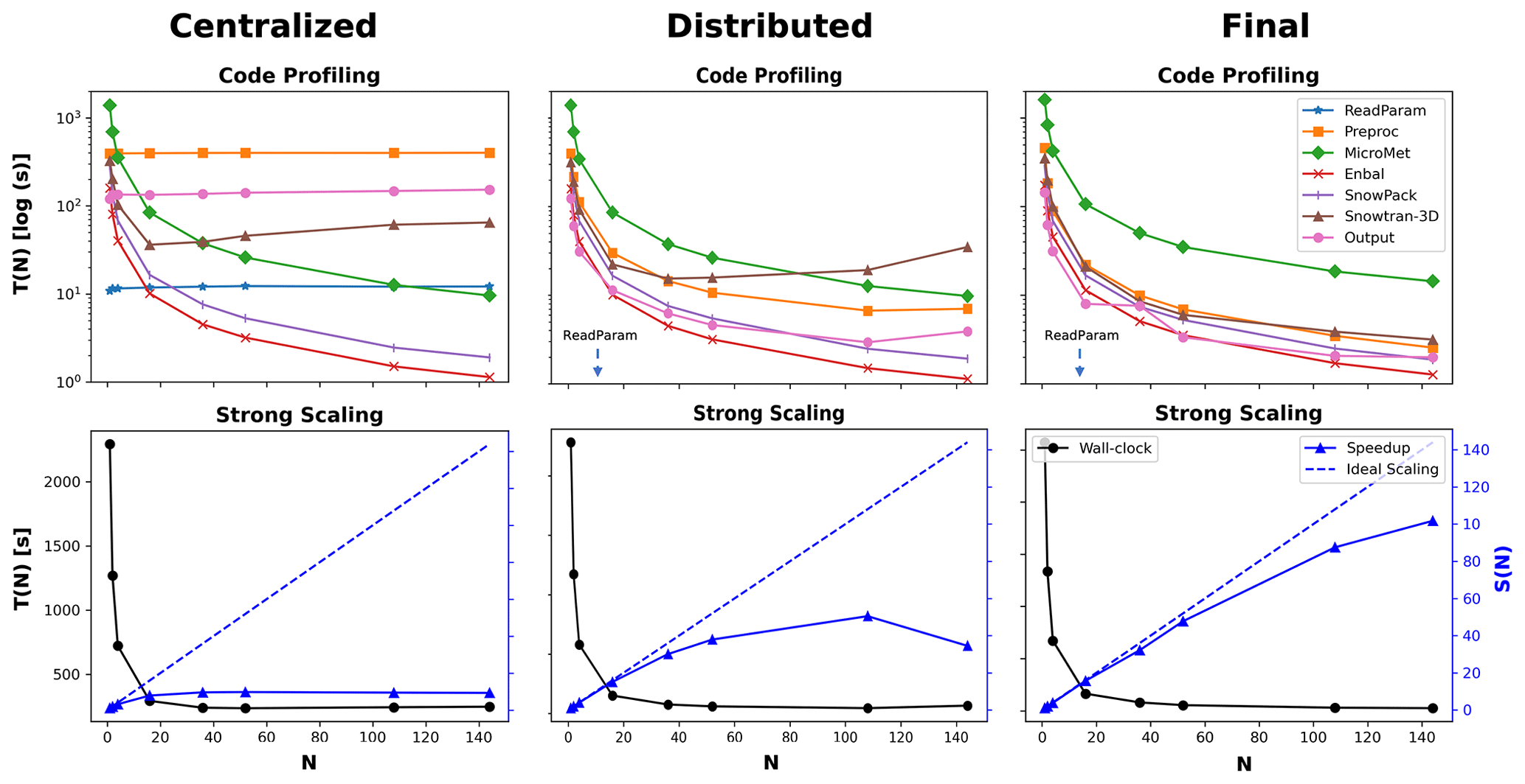
Figure 8Code profiling (top row) and strong scaling (bottom row) results demonstrating the progression of Parallel SnowModel, which includes a version of the code with centralized file I/O (centralized; first column), a version of the code with distributed file I/O (distributed; second column), and a final version of the code at the time of this publication (final; third column). These versions can be found as different commits within the GitHub repository (Mower et al., 2023). The code profiling plots display the cumulative execution time of each submodule on a logarithmic scale as a function of the number of processes (N). The arrow in the code profiling plots of distributed and final indicates the ReadParam timing is below the y axis at approximately 0.3 and 0.003 s, respectively. The strong scaling plots show the total execution time (T(N)) against N on the primary y axis and the speedup (S(N)) against N on the secondary y axis.
4.2 Strong scaling
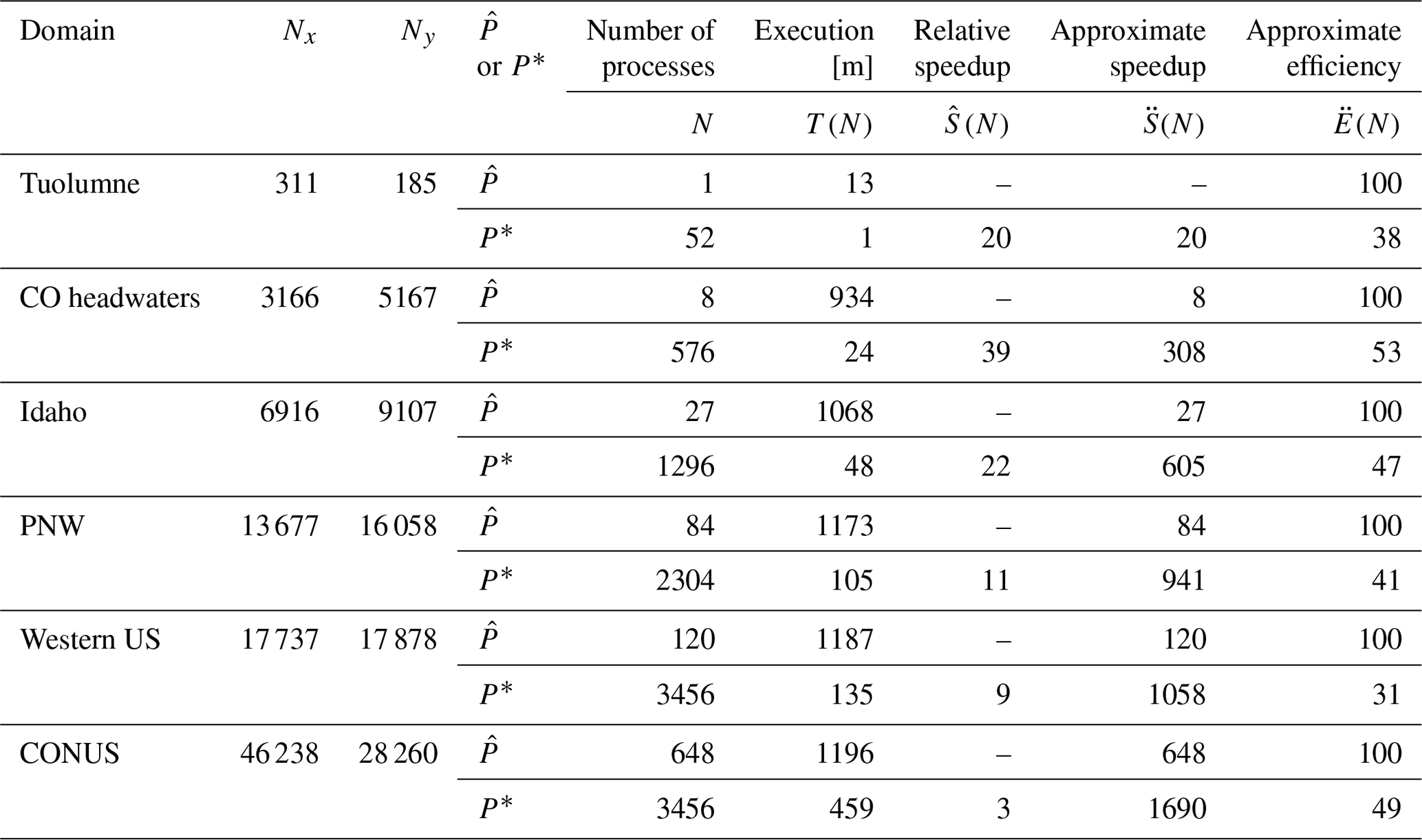
In addition to the parallel improvement analysis, strong scaling was also performed on six domains for the 2018 water year to better understand how Parallel SnowModel scales across different domain sizes and decompositions. Figure 9 displays the approximate speedup (; Eq. 3) of Parallel SnowModel for three local and/or state domains (Tuolumne, CO headwaters, and Idaho) and three regional and/or continental domains (PNW, western US, and CONUS). Additionally, Table 1 contains information about the minimum and maximum number of processors ( and P*, respectively) simulated on each domain and their corresponding execution time (T(N)[m]), relative speedup (; Eq. 2), approximate speedup (; Eq. 3), and approximate efficiency (; Eq. 5). As mentioned previously, simulations were constrained by both the 12 h wall-clock limit and 109 GB of memory per node on the Cheyenne supercomputer. In strong scaling, the number of processes is increased while the problem size remains constant; therefore, it represents a reduced workload per process. Local-sized domains, e.g., Tuolumne, likely do not warrant the need for parallel resources because they have small serial runtimes (e.g., using 52 processes, Tuolumne had an of 38 %; Table 1). However, state, regional, and continental domains stand to benefit more significantly from parallelization. The CONUS runtime decreased by a factor of 3 running on 3456 processes relative to 648 processes. Based on our approximate speedup assumption, we would estimate a CONUS of 1690 times on 3456 processes compared to one process, with an of 49 %. The western US and PNW domains display very similar scalability results (Fig. 9), which is attributed to the similar number of grid cells in the y dimension (Fig. 2 and Table 1) and thus parallel decomposition for each domain. Furthermore, these domains may also have a similar proportion of snow-covered grid cells. While the PNW likely has more terrestrial grid cells that are covered by snow for a longer period throughout the water year, it also has a significant number of ocean grid cells where snow redistribution would not be activated.
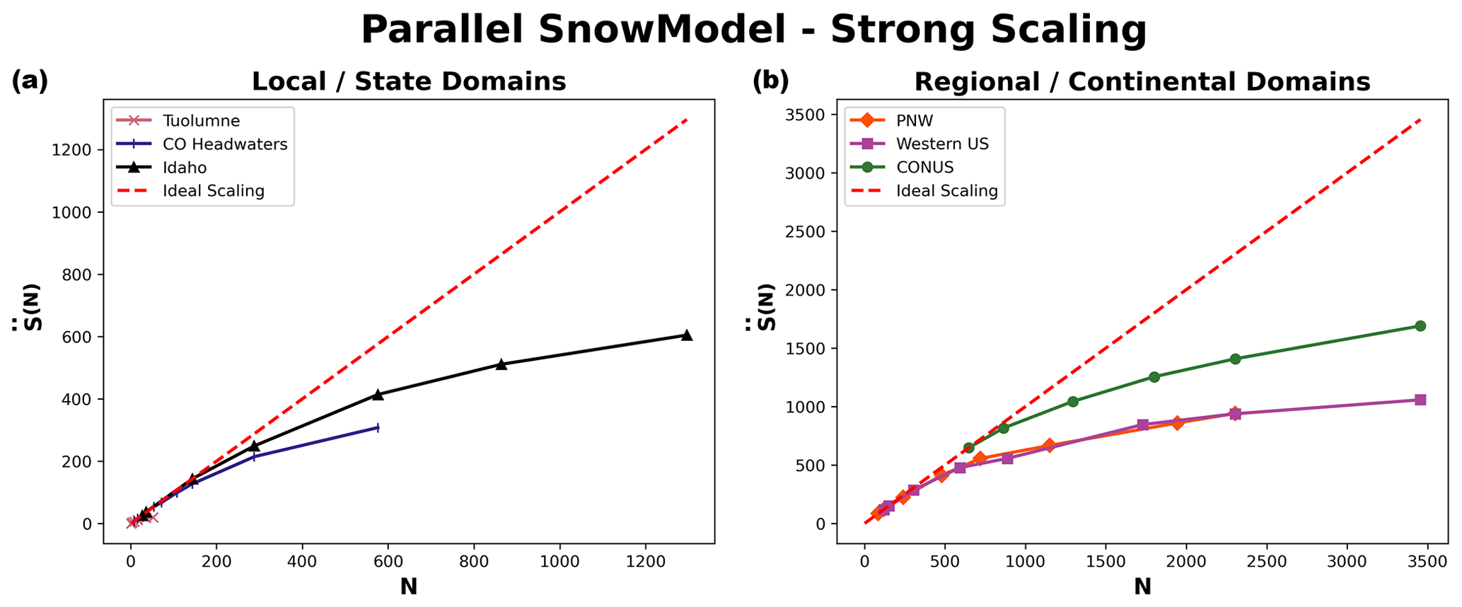
Figure 9Panel (a) displays approximate speedup () as a function of the number of processes (N) for local- and state-sized simulations (Tuolumne, CO headwaters, and Idaho), while panel (b) shows for regional- and continental-sized domains (PNW, western US, and CONUS).
Table 1Parallel SnowModel strong scaling results containing grid dimensions (Nx and Ny), execution time [m], relative speedup, approximate speedup, and approximate efficiency for simulations executed with the minimum and maximum number of processes ( and P*, respectively) on the Tuolumne, CO headwaters, Idaho, PNW, western US, and CONUS domains. Values of the timing, speedup, and efficiency variables are rounded to the nearest integer.
Strong scaling analysis is useful for I/O and memory-bound applications to identify a setup that results in a reasonable runtime and moderate resource costs. Based on these scaling results, Fig. 10 shows the relationship between the number of processes (N) at which each domain is estimated to reach 50 % (using linear interpolation) with the total number of grid cells in the y dimension (Ny) and the average number of grid cells in the y dimension per process (lny; inset Fig. 10). At this level of efficiency, the consistency of both the linear relationship between Ny and N (8.7:1 ratio) and the values of lny (5 to 11) for these year-long simulations that vary in both domain size and the proportion of snow-covered area is notable. Similar relationships (Fig. 10) can be used to approximate the scalability of Parallel SnowModel on different-sized domains and can be adjusted for the desired level of efficiency. For example, we decided to run the CONUS simulations (Sect. 4.3) using 1800 processes based on its 70 % approximate efficiency.
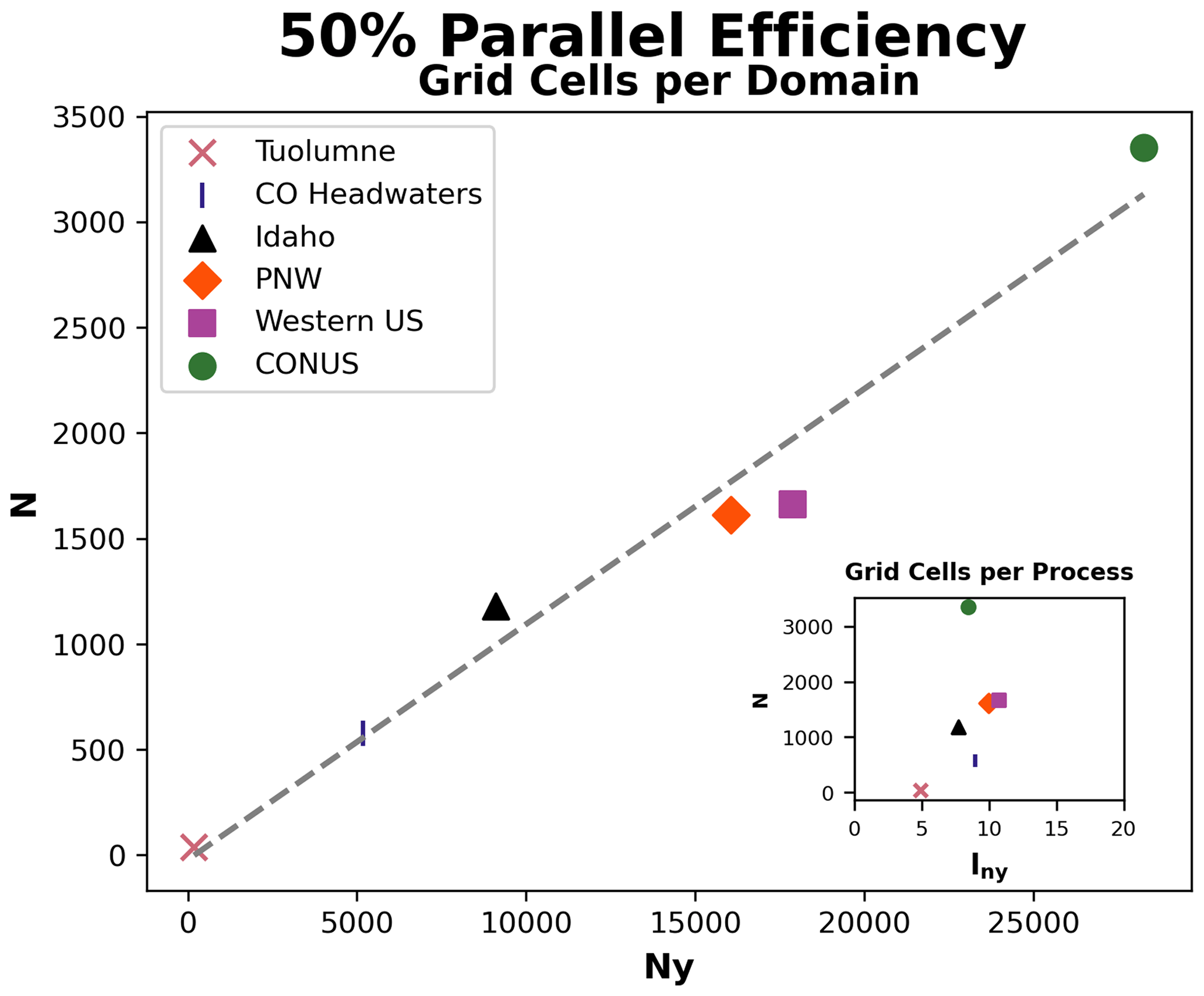
Figure 10Relationship between the number of grid cells in the y dimension (Ny) and the number of processes (N) for each domain at which 50 % approximate efficiency is estimated using the strong scaling analysis. The dashed line represents the best-fit line for this relationship using OLS regression. The inset figure displays a similar relationship but compares N to the average number of grid cells in the y dimension per process (lny) instead of Ny.
4.3 CONUS simulations
Spatial results of SWE on 12 February 2011 over the CONUS domain and a sub-domain located in the Indian Peaks west of Boulder, Colorado, are displayed in Fig. 11. On this date, simulated SWE was observed throughout the northern portion of the CONUS domain with the largest values concentrated in the mountain ranges (Fig. 11a). The Indian Peaks sub-domains of distributed SWE (Fig. 11b) with reference topography (Fig. 11c) underscore the ability of the large dataset to capture snow processes in a local alpine environment. It is important to note that while SnowModel does simulate snow redistribution, it does not currently have an avalanche model, which may be a limitation of accurately simulating SWE within this sub-domain. Additionally, Fig. 11b highlights two grid cells located 200 m apart on a peak. Figure 11d and e display the SWE evolution of these two grid cells over the entire dataset (water years 2000–2021) and the 2011 water year, respectively, further demonstrating the ability of Parallel SnowModel to capture fine-scale snow properties even when simulating continental domains. The upwind (western) grid cell is scoured by wind, and snow is transported to the downwind (eastern) grid cells where a snowdrift forms. The information and insight available in this high-resolution dataset will have important implications for many applications from hydrology, wildlife, and ecosystems to weather and climate and many more.
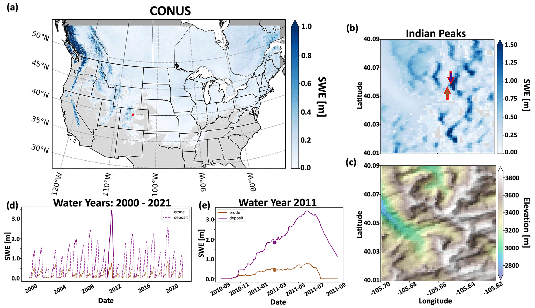
Figure 11Simulation results of Parallel SnowModel over CONUS using the WRF projection. (a) Spatial patterns of SWE over the CONUS domain for 12 February 2011, highlighting (b) the SWE distribution (c) and topography with an applied hillshade of a sub-domain near Apache Peak in the Indian Peaks west of Boulder, CO. (d) Time series of SWE from 2000–2021 and (e) over the 2011 water year for grid cells (“erode” and “deposit”) identified in panel (b). The erode and deposit grid cells highlight areas of similar elevation but significant differences in SWE evolution resulting from blowing snow redistribution processes.
Parallelizing numerical models often involves two-dimensional decomposition in both the x and y dimensions. While many benefits have been demonstrated by this approach, including improved load balancing (Dennis, 2007; Hamman et al., 2018), it comes with increased complication of the parallel algorithms, including the partitioning algorithm, file I/O, and process communication. The demonstrated speedup (Fig. 9) suggests Parallel SnowModel scales effectively over regional to continental domains using the one-dimensional decomposition approach. The added benefits obtained from two-dimensional decomposition strategies might not outweigh the costs of development, testing, and minimizing changes to the code structure and logic for applications such as SnowModel. Ultimately, our simplified parallelization approach can be implemented by other geoscience schemes as a first step to enhance simulation size and resolution.
Simulation experiments were conducted using Parallel SnowModel to validate the parallel logic, interpret its performance across different algorithm versions and domain sizes, and demonstrate its ability to simulate continental domains at high resolution. Code profiling and speedup analyses over the CO headwaters domain helped identify bottlenecks in file I/O and processor communication in SnowTran-3D during the development of the parallel algorithm (Sect. 4.1). Corrections to the referred bottlenecks allowed Parallel SnowModel to scale up to regional- and continental-sized simulations and highlights the value of optimizing scientific code. For Parallel SnowModel scalability is primarily dependent on the number of grid cells per process (Nx and lny) but is also affected by the proportion of snow-covered grid cells with sufficient winds and soft snow available to be redistributed (“Snow redistribution” section). The scalability analyses showed similar results across domains with significant differences in size (Nx and Ny), topography, vegetation, and snow classifications (Sturm et al., 1995; Sturm and Liston, 2021) (Sect. 4.2), highlighting the effectiveness of Parallel SnowModel for running state-, regional-, and continental-sized domains. Furthermore, results from this analysis can be used to estimate the number of processors required to simulate domains outside of the ones used in this study with a desired level of parallel efficiency (Fig. 10).
Additionally, these experiments emphasize the relationships among speed, memory, and computing resources for Parallel SnowModel. A common laptop (∼ 4 processes) has sufficient CPUs to run local-sized domains within a reasonable amount of time but likely does not have sufficient memory for state-sized simulations. Similarly, the minimum memory (1160 GB; Fig. 1) required to run the CONUS domain could be simulated on a large server (∼ 128 processes) with one process per node. However, extrapolating from our scaling results on Cheyenne (Fig. 9), we estimate it would take over 2.5 d to run a CONUS simulation for 1 water year with this configuration. In contrast, it took approximately 5 h for CONUS to run on the Discover supercomputer using 1800 processes. Therefore, by the time it took the large server to complete a CONUS simulation for 1 water year, 12 water years could have been simulated on a supercomputer. Lastly, results from the CONUS simulation highlight the ability of Parallel SnowModel to run high-resolution continental simulations, while maintaining fine-scale snow processes that occur at a local level (Sect. 4.3).
SnowModel can simulate high-resolution outputs of snow depth, density, SWE, grain size, thermal resistance, snow strength, snow albedo, landscape albedo, meltwater production, snow-water runoff, blowing snow flux, visibility, peak winter SWE, snow season length, snow onset date, snow-free date, and more, all produced by a physical model that maintains consistency among variables. While several snow data products exist, few capture the suite of snow properties along with the spatiotemporal extents and resolutions that can benefit a wide variety of applications. For example, current snow information products include the NASA daily SWE distributions globally for dry (non-melting) snow on a 25 km grid (Tedesco and Jeyaratnam, 2019), a NASA snow-cover product on a 500 m grid (Hall et al., 2006) that is missing information due to clouds approximately 50 % of the time (Moody et al., 2005), and the Snow Data Assimilation System (SNODAS) daily snow information provided by the National Oceanic and Atmospheric Administration (NOAA) and the National Weather Service (NWS) National Operational Hydrologic Remote Sensing Center (NOHRSC) on a 1 km grid (National Operational Hydrologic Remote Sensing Center, 2004), which is itself model-derived and has limited geographic coverage and snow properties. The Airborne Snow Observatory (ASO) provides the highest-resolution data with direct measurements of snow depth on a 3 m grid and derived values of SWE on a 50 m grid (Painter et al., 2016) but has limited spatiotemporal coverage and a high cost of acquisition. Furthermore, there are many fields of study that can benefit from 100 m resolution information on internally consistent snow variables, including wildlife and ecosystem, military, hydrology, weather and climate, cryosphere, recreation, remote sensing, engineering and civil works, and industrial applications. The new Parallel SnowModel described here permits the application of this modeling system to very large domains without sacrificing spatial resolution.
In this paper, we present a relatively simple parallelization approach that allows SnowModel to perform high-resolution simulations over regional- to continental-sized domains. The code within the core submodules (EnBal, MicroMet, SnowPack, and SnowTran-3D) and model configurations (single-layer snowpack, multi-layer snowpack, binary input files, etc.) was parallelized and modularized in this study. This allows SnowModel to be compiled with a range of Fortran compilers, including modern compilers that support parallel CAF either internally or through libraries, such as OpenCoarrays (Fanfarillo et al., 2014). Additionally, it provides the structure for other parallelization logic (e.g., MPI) to be more easily added to the code base. The parallel module contains a simple approach to decomposing the computational domain in the y dimension into smaller rectangular sub-domains. These sub-domains are distributed across processes to perform asynchronous calculations. The parallelization module also contains logic for communicating information among processes using halo-exchange coarrays for the wind and solar radiation models, as well as for snow redistribution. The scalability of Parallel SnowModel was demonstrated over different-sized domains, and the new code enables the creation of high-resolution simulated snow datasets on continental scales. This parallelization approach can be adopted in other parallelization efforts where spatial derivatives are calculated or fluxes are transported across gridded domains.
Some of the configuration combinations were not parallelized during this study for reasons including ongoing development in the serial code base and limitations to the parallelization approach. These include simulations involving tabler surfaces (Tabler, 1975), I/O using ASCII files, Lagrangian sea ice tracking, and data assimilation.
Validation SnowModel experiments were run in serial and in parallel over the Tuolumne and CO headwaters domains (Sect. 4.1) using the RMSE statistic. Important output variables from EnBal, MicroMet, SnowPack, and SnowTran-3D demonstrated similar, if not identical, values when compared to serial results for all time steps during the simulations; RMSE values were within machine precision (∼ 10−6) regardless of the output variable, domain, or number of processes used. The validated output variables include albedo [%], precipitation [m], emitted longwave radiation [W m−2], incoming longwave radiation reaching the surface [W m−2], incoming solar radiation reaching the surface [W m−2], relative humidity [%], runoff from the base of the snowpack [m ⋅ time step], rain precipitation [m], snow density [kg m−3], snow-water equivalent melt [m], snow depth [m], snow precipitation [m], static-surface sublimation [m], snow-water equivalent [m], air temperature [°C], wind direction [°], and wind speed [m s−1]. Ultimately, we feel confident that Parallel SnowModel is producing the same results as the original serial algorithm.
The Parallel SnowModel code and the data used in Sect. 4 are available through a public GitHub repository (https://github.com/NCAR/Parallel-SnowModel, Mower et al., 2023; https://doi.org/10.5281/zenodo.11168392, Mower, 2024). For more information about the serial version of SnowModel, refer to Liston and Elder (2006a). The data include figures and SnowModel output files that contain the necessary information to recreate the simulations. The gridded output variables themselves are not included due to storage limitations.
EDG and GDL conceived the study. RM, EDG, GDL, and SR were integral in the code development. RM, EDG, and JL were involved in the design, execution, and interpretation of the experiments. All authors discussed the results and contributed to the final version of the draft.
The contact author has declared that none of the authors has any competing interests.
Publisher’s note: Copernicus Publications remains neutral with regard to jurisdictional claims made in the text, published maps, institutional affiliations, or any other geographical representation in this paper. While Copernicus Publications makes every effort to include appropriate place names, the final responsibility lies with the authors.
We acknowledge Alessandro Fanfarillo for his help during the early stages of the Parallel SnowModel code development. We are also grateful for the feedback from various team members involved in the AIST project, including Carrie Vuyovich, Kristi Arsenault, Melissa Wrzesien, Adele Reinking, and Barton Forman.
This material is based upon work supported by the NSF National Center for Atmospheric Research, which is a major facility sponsored by the US National Science Foundation under cooperative agreement no. 1852977. We would also like to acknowledge computational support from the NSF NCAR Computational and Information Systems Lab (CISL) and the NASA High-End Computing (HEC) program through the NASA Center for Climate Simulation (NCCS) at Goddard Space Flight Center.
This research has been supported by the NASA Earth Science Office (ESTO) Advanced Information Systems Technology (AIST) program (grant no. 80NSSC20K0207), the University of Washington's College of Engineering Fellowship, and the US National Science Foundation (grant no. 1852977).
This paper was edited by Lele Shu and reviewed by three anonymous referees.
Beniston, M.: Climatic Change in Mountain Regions: A Review of Possible Impacts, Climatic Change, 59, 5–31, https://doi.org/10.1023/A:1024458411589, 2003.
Bernhardt, M., Schulz, K., Liston, G. E., and Zängl, G.: The influence of lateral snow redistribution processes on snow melt and sublimation in alpine regions, J. Hydrol., 424–425, 196–206, https://doi.org/10.1016/j.jhydrol.2012.01.001, 2012.
Boelman, N. T., Liston, G. E., Gurarie, E., Meddens, A. J. H., Mahoney, P. J., Kirchner, P. B., Bohrer, G., Brinkman, T. J., Cosgrove, C. L., Eitel, J. U. H., Hebblewhite, M., Kimball, J. S., LaPoint, S., Nolin, A. W., Pedersen, S. H., Prugh, L. R., Reinking, A. K., and Vierling, L. A.: Integrating snow science and wildlife ecology in Arctic-boreal North America, Environ. Res. Lett., 14, 010401, https://doi.org/10.1088/1748-9326/aaeec1, 2019.
Clark, M. P. and Hay, L. E.: Use of Medium-Range Numerical Weather Prediction Model Output to Produce Forecasts of Streamflow, J. Hydrometeorol., 5, 15–32, https://doi.org/10.1175/1525-7541(2004)005<0015:Uomnwp>2.0.Co;2, 2004.
Coarfa, C., Dotsenko, Y., Mellor-Crummey, J., Cantonnet, F., El-Ghazawi, T., Mohanti, A., Yao, Y., and Chavarría-Miranda, D.: An evaluation of global address space languages: co-array fortran and unified parallel c, Proceedings of the tenth ACM SIGPLAN symposium on Principles and practice of parallel programming, 36–47, https://doi.org/10.1145/1065944.1065950, 2005.
Computational and Information Systems Laboratory: Cheyenne: HPE/SGI ICE XA System (NCAR Community Computing), National Center for Atmospheric Research, Boulder, CO, https://doi.org/10.5065/D6RX99HX, 2019.
Dennis, J. M.: Inverse space-filling curve partitioning of a global ocean model, 2007 IEEE International Parallel and Distributed Processing Symposium, 1–10, https://doi.org/10.1109/IPDPS.2007.370215, 2007.
Dozier, J., Bair, E. H., and Davis, R. E.: Estimating the spatial distribution of snow water equivalent in the world's mountains, WIREs Water, 3, 461–474, https://doi.org/10.1002/wat2.1140, 2016.
Essery, R., Li, L., and Pomeroy, J.: A distributed model of blowing snow over complex terrain, Hydrol. Process., 13, 2423–2438, https://doi.org/10.1002/(SICI)1099-1085(199910)13:14/15<2423::AID-HYP853>3.0.CO;2-U, 1999.
Fanfarillo, A., Burnus, T., Cardellini, V., Filippone, S., Nagle, D., and Rouson, D.: OpenCoarrays: open-source transport layers supporting coarray Fortran compilers, Proceedings of the 8th International Conference on Partitioned Global Address Space Programming Models, 1–11, https://doi.org/10.1145/2676870.2676876, 2014.
Fang, X. and Pomeroy, J.: Modeling blowing snow redistribution to prairie wetlands, Hydrol. Process., 23, 2557–2569, https://doi.org/10.1002/hyp.7348, 2009.
Foster, J. L., Hall, D. K., Eylander, J. B., Riggs, G. A., Nghiem, S. V., Tedesco, M., Kim, E., Montesano, P. M., Kelly, R. E. J., Casey, K. A., and Choudhury, B.: A blended global snow product using visible, passive microwave and scatterometer satellite data, Int. J. Remote Sens., 32, 1371–1395, https://doi.org/10.1080/01431160903548013, 2011.
Freudiger, D., Kohn, I., Seibert, J., Stahl, K., and Weiler, M.: Snow redistribution for the hydrological modeling of alpine catchments, WIREs Water, 4, e1232, https://doi.org/10.1002/wat2.1232, 2017.
Gesch, D. B., Evans, G. A., Oimoen, M. J., and Arundel, S.: The National Elevation Dataset, edited by: United States Geological Survey, American Society for Photogrammetry and Remote Sensing, 83–110, 2018.
Hall, D. K., Salomonson, V. V., and Riggs, G. A.: MODIS/Terra Snow Cover 5-Min L2 Swath 500m, Version 5, Boulder, Colorado USA, NASA National Snow and Ice Data Center Distributed Active Archive Center, https://doi.org/10.5067/ACYTYZB9BEOS, 2006.
Hamman, J. J., Nijssen, B., Bohn, T. J., Gergel, D. R., and Mao, Y.: The Variable Infiltration Capacity model version 5 (VIC-5): infrastructure improvements for new applications and reproducibility, Geosci. Model Dev., 11, 3481–3496, https://doi.org/10.5194/gmd-11-3481-2018, 2018.
Hammond, J. C., Sexstone, G. A., Putman, A. L., Barnhart, T. B., Rey, D. M., Driscoll, J. M., Liston, G. E., Rasmussen, K. L., McGrath, D., Fassnacht, S. R., and Kampf, S. K.: High Resolution SnowModel Simulations Reveal Future Elevation-Dependent Snow Loss and Earlier, Flashier Surface Water Input for the Upper Colorado River Basin, Earth's Future, 11, e2022EF003092, https://doi.org/10.1029/2022EF003092, 2023.
Homer, C., Dewitz, J., Yang, L., Jin, S., Danielson, P., Xian, G., Coulston, J., Herold, N., Wickham, J., and Megown, K.: Completion of the 2011 National Land Cover Database for the conterminous United States–representing a decade of land cover change information, Photogramm. Eng. Remote Sens., 81, 345–354, 2015.
Hoppinen, Z., Oveisgharan, S., Marshall, H.-P., Mower, R., Elder, K., and Vuyovich, C.: Snow water equivalent retrieval over Idaho – Part 2: Using L-band UAVSAR repeat-pass interferometry, The Cryosphere, 18, 575–592, https://doi.org/10.5194/tc-18-575-2024, 2024.
Huss, M., Bookhagen, B., Huggel, C., Jacobsen, D., Bradley, R. S., Clague, J. J., Vuille, M., Buytaert, W., Cayan, D. R., Greenwood, G., Mark, B. G., Milner, A. M., Weingartner, R., and Winder, M.: Toward mountains without permanent snow and ice, Earth's Future, 5, 418–435, https://doi.org/10.1002/2016EF000514, 2017.
Immerzeel, W. W., Lutz, A. F., Andrade, M., Bahl, A., Biemans, H., Bolch, T., Hyde, S., Brumby, S., Davies, B. J., Elmore, A. C., Emmer, A., Feng, M., Fernández, A., Haritashya, U., Kargel, J. S., Koppes, M., Kraaijenbrink, P. D. A., Kulkarni, A. V., Mayewski, P. A., Nepal, S., Pacheco, P., Painter, T. H., Pellicciotti, F., Rajaram, H., Rupper, S., Sinisalo, A., Shrestha, A. B., Viviroli, D., Wada, Y., Xiao, C., Yao, T., and Baillie, J. E. M.: Importance and vulnerability of the world's water towers, Nature, 577, 364–369, https://doi.org/10.1038/s41586-019-1822-y, 2020.
ISO/IEC: Fortran Standard 2008, Technical report, Geneva, Switzerland, https://j3-fortran.org/doc/year/10/10-007.pdf (last access: 10 July 2023), 2010.
Jin, S., Homer, C., Yang, L., Danielson, P., Dewitz, J., Li, C., Zhu, Z., Xian, G., and Howard, D.: Overall methodology design for the United States national land cover database 2016 products, Remote Sens., 11, 2971, https://doi.org/10.3390/rs11242971, 2019.
Keenan, E., Wever, N., Lenaerts, J. T. M., and Medley, B.: A wind-driven snow redistribution module for Alpine3D v3.3.0: adaptations designed for downscaling ice sheet surface mass balance, Geosci. Model Dev., 16, 3203–3219, https://doi.org/10.5194/gmd-16-3203-2023, 2023.
Kumar, V. and Gupta, A.: Analysis of scalability of parallel algorithms and architectures: A survey, Proceedings of the 5th international conference on Supercomputing, 396–405, https://doi.org/10.1006/jpdc.1994.1099, 1991.
Latifovic, R., Homer, C., Ressl, R., Pouliot, D., Hossain, S. N., Colditz, R. R., Olthof, I., Giri, C. P., and Victoria, A.: 20 North American Land-Change Monitoring System, Remote sensing of land use and land cover, CRC Press, 303, https://doi.org/10.1201/b11964-24, 2016.
Lehning, M., Völksch, I., Gustafsson, D., Nguyen, T., Stähli, M., and Zappa, M.: ALPINE3D: A detailed model of mountain surface processes and its application to snow hydrology, Hydrol. Process., 20, 2111–2128, https://doi.org/10.1002/hyp.6204, 2006.
Lehning, M., Löwe, H., Ryser, M., and Raderschall, N.: Inhomogeneous precipitation distribution and snow transport in steep terrain, Water Resour. Res., 44, W07404, https://doi.org/10.1029/2007WR006545, 2008.
Lettenmaier, D. P., Alsdorf, D., Dozier, J., Huffman, G. J., Pan, M., and Wood, E. F.: Inroads of remote sensing into hydrologic science during the WRR era, Water Resour. Res., 51, 7309–7342, https://doi.org/10.1002/2015WR017616, 2015.
Liston, G. E.: Local advection of momentum, heat, and moisture during the melt of patchy snow covers, J. Appl. Meteorol. Clim., 34, 1705–1715, 1995.
Liston, G. E.: Representing Subgrid Snow Cover Heterogeneities in Regional and Global Models, J. Climate, 17, 1381–1397, https://doi.org/10.1175/1520-0442(2004)017<1381:Rsschi>2.0.Co;2, 2004.
Liston, G. E. and Elder, K.: A distributed snow-evolution modeling system (SnowModel), J. Hydrometeorol., 7, 1259–1276, 2006a.
Liston, G. E. and Elder, K.: A Meteorological Distribution System for High-Resolution Terrestrial Modeling (MicroMet), J. Hydrometeorol., 7, 217–234, https://doi.org/10.1175/jhm486.1, 2006b.
Liston, G. E. and Hall, D. K.: An energy-balance model of lake-ice evolution, J. Glaciol., 41, 373–382, 1995.
Liston, G. E. and Hiemstra, C. A.: A simple data assimilation system for complex snow distributions (SnowAssim), J. Hydrometeorol., 9, 989–1004, 2008.
Liston, G. E. and Hiemstra, C. A.: The changing cryosphere: Pan-Arctic snow trends (1979–2009), J. Climate, 24, 5691–5712, 2011.
Liston, G. E. and Mernild, S. H.: Greenland freshwater runoff. Part I: A runoff routing model for glaciated and nonglaciated landscapes (HydroFlow), J. Climate, 25, 5997–6014, 2012.
Liston, G. E. and Sturm, M.: A snow-transport model for complex terrain, J. Glaciol., 44, 498–516, 1998.
Liston, G. E. and Sturm, M.: Global Seasonal-Snow Classification, Version 1, NASA National Snow and Ice Data Center Distributed Active Archive Center [data set], https://doi.org/10.5067/99FTCYYYLAQ0, 2021.
Liston, G. E., Winther, J.-G., Bruland, O., Elvehøy, H., and Sand, K.: Below-surface ice melt on the coastal Antarctic ice sheet, J. Glaciol., 45, 273–285, 1999.
Liston, G. E., Haehnel, R. B., Sturm, M., Hiemstra, C. A., Berezovskaya, S., and Tabler, R. D.: Simulating complex snow distributions in windy environments using SnowTran-3D, J. Glaciol., 53, 241–256, 2007.
Liston, G. E., Perham, C. J., Shideler, R. T., and Cheuvront, A. N.: Modeling snowdrift habitat for polar bear dens, Ecol. Model., 320, 114–134, https://doi.org/10.1016/j.ecolmodel.2015.09.010, 2016.
Liston, G. E., Polashenski, C., Rösel, A., Itkin, P., King, J., Merkouriadi, I., and Haapala, J.: A distributed snow-evolution model for sea-ice applications (SnowModel), J. Geophys. Res.-Oceans, 123, 3786–3810, 2018.
Liston, G. E., Itkin, P., Stroeve, J., Tschudi, M., Stewart, J. S., Pedersen, S. H., Reinking, A. K., and Elder, K.: A Lagrangian snow-evolution system for sea-ice applications (SnowModel-LG): Part I – Model description, J. Geophys. Res-Oceans, 125, e2019JC015913, https://doi.org/10.1029/2019JC015913, 2020.
Liston, G. E., Reinking, A. K., and Boleman, N. T.: Daily SnowModel Outputs Covering the ABoVE Core Domain, 3-km Resolution, 1980–2020, ORNL DAAC, Oak Ridge, Tennessee, USA, https://doi.org/10.3334/ORNLDAAC/2105, 2023.
Lund, J., Forster, R. R., Deeb, E. J., Liston, G. E., Skiles, S. M., and Marshall, H.-P.: Interpreting Sentinel-1 SAR Backscatter Signals of Snowpack Surface Melt/Freeze, Warming, and Ripening, through Field Measurements and Physically-Based SnowModel, Remote Sens., 14, 4002, https://doi.org/10.3390/rs14164002, 2022.
Mahoney, P. J., Liston, G. E., LaPoint, S., Gurarie, E., Mangipane, B., Wells, A. G., Brinkman, T. J., Eitel, J. U., Hebblewhite, M., and Nolin, A. W.: Navigating snowscapes: scale-dependent responses of mountain sheep to snowpack properties, Ecol. Appl., 28, 1715–1729, 2018.
Marsh, C. B., Pomeroy, J. W., Spiteri, R. J., and Wheater, H. S.: A Finite Volume Blowing Snow Model for Use With Variable Resolution Meshes, Water Resour. Res., 56, e2019WR025307, https://doi.org/10.1029/2019WR025307, 2020.
Miller, P., Robson, M., El-Masri, B., Barman, R., Zheng, G., Jain, A., and Kalé, L.: Scaling the isam land surface model through parallelization of inter-component data transfer, 2014 43rd International Conference on Parallel Processing, 422–431, https://doi.org/10.1109/ICPP.2014.51, 2014.
Mitchell, K. E.: The multi-institution North American Land Data Assimilation System (NLDAS): Utilizing multiple GCIP products and partners in a continental distributed hydrological modeling system, J. Geophys. Res., 109, D07S90, https://doi.org/10.1029/2003JD003823, 2004.
Moody, E. G., King, M. D., Platnick, S., Schaaf, C. B., and Gao, F.: Spatially complete global spectral surface albedos: Value-added datasets derived from Terra MODIS land products, IEEE T. Geosci. Remote Sens., 43, 144–158, 2005.
Morin, S., Horton, S., Techel, F., Bavay, M., Coléou, C., Fierz, C., Gobiet, A., Hagenmuller, P., Lafaysse, M., Ližar, M., Mitterer, C., Monti, F., Müller, K., Olefs, M., Snook, J. S., van Herwijnen, A., and Vionnet, V.: Application of physical snowpack models in support of operational avalanche hazard forecasting: A status report on current implementations and prospects for the future, Cold Reg. Sci. Technol., 170, 102910, https://doi.org/10.1016/j.coldregions.2019.102910, 2020.
Mortezapour, M., Menounos, B., Jackson, P. L., Erler, A. R., and Pelto, B. M.: The role of meteorological forcing and snow model complexity in winter glacier mass balance estimation, Columbia River basin, Canada, Hydrol. Process., 34, 5085–5103, https://doi.org/10.1002/hyp.13929, 2020.
Mott, R. and Lehning, M.: Meteorological Modeling of Very High-Resolution Wind Fields and Snow Deposition for Mountains, J. Hydrometeorol., 11, 934–949, https://doi.org/10.1175/2010JHM1216.1, 2010.
Mott, R., Schirmer, M., Bavay, M., Grünewald, T., and Lehning, M.: Understanding snow-transport processes shaping the mountain snow-cover, The Cryosphere, 4, 545–559, https://doi.org/10.5194/tc-4-545-2010, 2010.
Mower, R.: NCAR/Parallel-SnowModel: Parallel-SnowModel (v1.0.0), Zenodo [code], https://doi.org/10.5281/zenodo.11168392, 2024.
Mower, R., Gutmann, E. D., and Liston, G. E.: Parallel-SnowModel, Github [data set and code], https://github.com/NCAR/Parallel-SnowModel (last access: 31 January 2024), 2023.
Mudryk, L. R., Derksen, C., Kushner, P. J., and Brown, R.: Characterization of Northern Hemisphere Snow Water Equivalent Datasets, 1981–2010, J. Climate, 28, 8037–8051, https://doi.org/10.1175/jcli-d-15-0229.1, 2015.
National Operational Hydrologic Remote Sensing Center: Snow Data Assimilation System (SNODAS) Data Products at NSIDC, Version 1, Boulder, Colorado USA, NSIDC: National Snow and Ice Data Center, https://doi.org/10.7265/N5TB14TC, 2004.
Nolin, A. W.: Recent advances in remote sensing of seasonal snow, J. Glaciol., 56, 1141–1150, https://doi.org/10.3189/002214311796406077, 2010.
Numrich, R. W. and Reid, J.: Co-Array Fortran for parallel programming, ACM Sigplan Fortran Forum, 1–31, https://doi.org/10.1145/289918.289920, 1998.
Numrich, R. W., Steidel, J. L., Johnson, B. H., Dinechin, B. D. d., Elsesser, G., Fischer, G., and MacDonald, T.: Definition of the F– Extension to Fortran 90, International Workshop on Languages and Compilers for Parallel Computing, 292–306, https://doi.org/10.1007/BFb0032700, 1998.
Painter, T. H., Berisford, D. F., Boardman, J. W., Bormann, K. J., Deems, J. S., Gehrke, F., Hedrick, A., Joyce, M., Laidlaw, R., and Marks, D.: The Airborne Snow Observatory: Fusion of scanning lidar, imaging spectrometer, and physically-based modeling for mapping snow water equivalent and snow albedo, Remote Sens. Environ., 184, 139–152, 2016.
Parhami, B.: SIMD machines: do they have a significant future?, ACM SIGARCH Computer Architecture News, 23, 19–22, 1995.
Pedersen, S. H., Liston, G. E., Tamstorf, M. P., Westergaard-Nielsen, A., and Schmidt, N. M.: Quantifying Episodic Snowmelt Events in Arctic Ecosystems, Ecosystems, 18, 839–856, https://doi.org/10.1007/s10021-015-9867-8, 2015.
Pedersen, S. H., Liston, G. E., Tamstorf, M. P., Schmidt, N. M., and Abermann, J.: Linking vegetation greenness and seasonal snow characteristics using field observations, SnowModel, and daily MODIS imagery in high-Arctic Greenland, AGU Fall Meeting Abstracts, GC42A-07, https://ui.adsabs.harvard.edu/abs/2016AGUFMGC42A..07P/abstract (last access: 16 October 2023), 2016.
Perezhogin, P., Chernov, I., and Iakovlev, N.: Advanced parallel implementation of the coupled ocean–ice model FEMAO (version 2.0) with load balancing, Geosci. Model Dev., 14, 843–857, https://doi.org/10.5194/gmd-14-843-2021, 2021.
Pflug, J. M. and Lundquist, J. D.: Inferring Distributed Snow Depth by Leveraging Snow Pattern Repeatability: Investigation Using 47 Lidar Observations in the Tuolumne Watershed, Sierra Nevada, California, Water Resour. Res., 56, e2020WR027243, https://doi.org/10.1029/2020WR027243, 2020.
Prokop, A. and Schneiderbauer, S.: The atmospheric snow-transport model: SnowDrift3D, J. Glaciol., 57, 526–542, https://doi.org/10.3189/002214311796905677, 2011.
Quéno, L., Mott, R., Morin, P., Cluzet, B., Mazzotti, G., and Jonas, T.: Snow redistribution in an intermediate-complexity snow hydrology modelling framework, EGUsphere [preprint], https://doi.org/10.5194/egusphere-2023-2071, 2023.
Randin, C. F., Dedieu, J.-P., Zappa, M., Long, L., and Dullinger, S.: Validation of and comparison between a semidistributed rainfall–runoff hydrological model (PREVAH) and a spatially distributed snow-evolution model (SnowModel) for snow cover prediction in mountain ecosystems, Ecohydrology, 8, 1181–1193, https://doi.org/10.1002/eco.1570, 2015.
Rasmussen, R. M., Liu, C., Ikeda, K., Chen, F., Kim, J.-H., Schneider, T., Gochis, D., Dugger, A., and Viger, R.: Four-kilometer long-term regional hydroclimate reanalysis over the conterminous United States (CONUS), 1979–2020, Research Data Archive at the National Center for Atmospheric Research, Computational and Information Systems Laboratory [data set], https://doi.org/10.5065/ZYY0-Y036, 2023.
Renwick, J.: MOUNTerrain: GEWEX mountainous terrain precipitation project, GEWEX News, 24, 5–6, 2014.
Reynolds, D. S., Pflug, J. M., and Lundquist, J. D.: Evaluating wind fields for use in basin-scale distributed snow models, Water Resour. Res., 57, e2020WR028536, https://doi.org/10.1029/2020WR028536, 2021.
Richter, B., Schweizer, J., Rotach, M. W., and van Herwijnen, A.: Modeling spatially distributed snow instability at a regional scale using Alpine3D, J. Glaciol., 67, 1147–1162, https://doi.org/10.1017/jog.2021.61, 2021.
Rouson, D., Gutmann, E. D., Fanfarillo, A., and Friesen, B.: Performance portability of an intermediate-complexity atmospheric research model in coarray Fortran, Proceedings of the Second Annual PGAS Applications Workshop, 1–4, https://doi.org/10.1145/3144779.3169104, 2017.
Skofronick-Jackson, G. M., Johnson, B. T., and Munchak, S. J.: Detection Thresholds of Falling Snow From Satellite-Borne Active and Passive Sensors, IEEE T. Geosci. Remote S., 51, 4177–4189, https://doi.org/10.1109/TGRS.2012.2227763, 2013.
Sturm, M. and Liston, G. E.: Revisiting the global seasonal snow classification: An updated dataset for earth system applications, J. Hydrometeorol., 22, 2917–2938, 2021.
Sturm, M., Holmgren, J., and Liston, G. E.: A Seasonal Snow Cover Classification System for Local to Global Applications, J. Climate, 8, 1261–1283, https://doi.org/10.1175/1520-0442(1995)008<1261:Assccs>2.0.Co;2, 1995.
Szczypta, C., Gascoin, S., Houet, T., and Fanise, P.: Impact of climate versus land-use changes on snow cover in Bassiès, Pyrenees, International Snow Science Workshop Grenoble â Chamonix Mont-Blanc, 1278–1281, https://api.semanticscholar.org/CorpusID:55357771 (last access: 15 January 2024), 2013.
Tabler, R. D.: Estimating the transport and evaporation of blowing snow, Great Plains Agric. Council, Nebraska Univ., Publ., 73, 85–104, 1975.
Takala, M., Luojus, K., Pulliainen, J., Derksen, C., Lemmetyinen, J., Kärnä, J.-P., Koskinen, J., and Bojkov, B.: Estimating northern hemisphere snow water equivalent for climate research through assimilation of space-borne radiometer data and ground-based measurements, Remote Sens. Environ., 115, 3517–3529, https://doi.org/10.1016/j.rse.2011.08.014, 2011.
Tedesco, M. and Jeyaratnam, J.: AMSR-E/AMSR2 Unified L3 Global Daily 25 km EASE-Grid Snow Water Equivalent, Version 1, Boulder, Colorado USA, NASA National Snow and Ice Data Center Distributed Active Archive Center, https://doi.org/10.5067/8AE2ILXB5SM6, 2019.
Vionnet, V., Martin, E., Masson, V., Guyomarc'h, G., Naaim-Bouvet, F., Prokop, A., Durand, Y., and Lac, C.: Simulation of wind-induced snow transport and sublimation in alpine terrain using a fully coupled snowpack/atmosphere model, The Cryosphere, 8, 395–415, https://doi.org/10.5194/tc-8-395-2014, 2014.
Vionnet, V., Martin, E., Masson, V., Lac, C., Naaim Bouvet, F., and Guyomarc'h, G.: High-resolution large eddy simulation of snow accumulation in Alpine terrain, J. Geophys. Res.-Atmos., 122, 11005–11021, 2017.
Voordendag, A., Réveillet, M., MacDonell, S., and Lhermitte, S.: Snow model comparison to simulate snow depth evolution and sublimation at point scale in the semi-arid Andes of Chile, The Cryosphere, 15, 4241–4259, https://doi.org/10.5194/tc-15-4241-2021, 2021.
Vuyovich, C. M., Jacobs, J. M., and Daly, S. F.: Comparison of passive microwave and modeled estimates of total watershed SWE in the continental United States, Water Resour. Res., 50, 9088–9102, https://doi.org/10.1002/2013WR014734, 2014.
Wagner, C., Hunsaker, A., and Jacobs, J.: UAV and SnowModel Estimates of Wind Driven Snow in Eastern USA Avalanche Terrain, EGU General Assembly 2023, Vienna, Austria, 23–28 Apr 2023, EGU23-4608, https://doi.org/10.5194/egusphere-egu23-4608, 2023.
Wrzesien, M. L., Durand, M. T., Pavelsky, T. M., Kapnick, S. B., Zhang, Y., Guo, J., and Shum, C. K.: A New Estimate of North American Mountain Snow Accumulation From Regional Climate Model Simulations, Geophys. Res. Lett., 45, 1423–1432, https://doi.org/10.1002/2017GL076664, 2018.
Xia, Y.: Continental-scale water and energy flux analysis and validation for North American Land Data Assimilation System project phase 2 (NLDAS-2): 1. Intercomparison and application of model products, J. Geophys. Res., 117, D03109, https://doi.org/10.1029/2011JD016048, 2012a.
Xia, Y.: Continental-scale water and energy flux analysis and validation for North American Land Data Assimilation System project phase 2 (NLDAS-2): 2. Validation of model-simulated streamflow, J. Geophys. Res., 117, D03110, https://doi.org/10.1029/2011JD016051, 2012b.
Xue, M., Droegemeier, K. K., and Wong, V.: The Advanced Regional Prediction System (ARPS) – A multi-scale nonhydrostatic atmospheric simulation and prediction model. Part I: Model dynamics and verification, Meteorol. Atmos. Phys., 75, 161–193, https://doi.org/10.1007/s007030070003, 2000.