the Creative Commons Attribution 4.0 License.
the Creative Commons Attribution 4.0 License.
 | 16 Jan 2024
GAN-argcPredNet v2.0: a radar echo extrapolation model based on spatiotemporal process enhancement
Qiya Tan
Huihua Ruan
Jinbiao Zhang
Cong Luo
Siyu Tang
Yunlei Yi
Yugang Tian
Jianmei Cheng
Precipitation nowcasting has important implications for urban operation and flood prevention. Radar echo extrapolation is a common method in precipitation nowcasting. Using deep learning models to extrapolate radar echo data has great potential. The increase of lead time leads to a weaker correlation between the real rainfall evolution and the generated images. The evolution information is easily lost during extrapolation, which is reflected as echo attenuation. Existing models, including generative adversarial network (GAN)-based models, have difficulty curbing attenuation, resulting in insufficient accuracy in rainfall prediction. To solve this issue, a spatiotemporal process enhancement network (GAN-argcPredNet v2.0) based on GAN-argcPredNet v1.0 has been designed. GAN-argcPredNet v2.0 curbs attenuation by avoiding blurring or maintaining the intensity. A spatiotemporal image correlation (STIC) prediction network is designed as the generator. By suppressing the blurring effect of rain distribution and reducing the negative bias by STIC attention, the generator generates more accurate images. Furthermore, the discriminator is a channel–spatial (CS) convolution network. The discriminator enhances the discrimination of echo information and provides better guidance to the generator in image generation by CS attention. The experiments are based on the radar dataset of southern China. The results show that GAN-argcPredNet v2.0 performs better than other models. In heavy rainfall prediction, compared with the baseline, the probability of detection (POD), the critical success index (CSI), the Heidke skill score (HSS) and bias score increase by 18.8 %, 17.0 %, 17.2 % and 26.3 %, respectively. The false alarm ratio (FAR) decreases by 3.0 %.
- Article
(8255 KB) - Full-text XML
-
Supplement
(335 KB) - BibTeX
- EndNote


Accurate precipitation nowcasting, especially heavy precipitation nowcasting, plays a key role in hydrometeorological applications such as urban operation safety and flash-flood warnings (Liu et al., 2015). It can effectively prevent hazards and losses caused by heavy precipitation to the economy and people (Luo et al., 2020). Radar echo extrapolation is the method most often used to nowcast precipitation (Reyniers, 2008). The essence is tracking areas of reflectivity to derive motion vectors and then using the motion vectors to determine the future location of the reflectivity (Austin and Bellon, 1974).
Traditional radar echo extrapolation methods include cross-correlation, individual radar echo tracking and the optical flow method (Bowler et al., 2004). Thunderstorm Identification, Tracking, Analysis and Nowcasting (TITAN) is a classical centroid tracking algorithm (Dixon and Wiener, 1993). This algorithm achieves precipitation nowcasting by real-time tracking and automatic identification of individual storms. However, the tracking performance of TITAN is poor during multi-cell storms. To address this, an enhanced TITAN (ETITAN) was proposed (Han et al., 2009). By combining cross-correlation and individual radar echo tracking, ETITAN achieves more accurate tracking and prediction. While the cross-correlation method is effective, it has lower prediction accuracy when echoes change rapidly. On the other hand, the optical flow method achieves local prediction by treating echo motion as fluid (Sakaino, 2013). Additionally, some traditional nowcasting systems combine different information and further improve the ability of nowcasting. A Bayesian precipitation nowcasting system based on the ensemble Kalman filter was formulated. The system correctly captures the flow dependence of both the numerical weather prediction (NWP) forecast and the Lagrangian persistence of radar observations (Nerini et al., 2019). Furthermore, the variational algorithm is used to improve the nowcasting system to achieve 3 h nowcasting (Chung and Yao, 2020). The Lagrangian INtegro-Difference equation model with Autoregression (LINDA) also performs better for prediction accuracy and duration (Pulkkinen et al., 2021). As the storm evolves in ways such as merging, splitting, growth and decay, traditional methods are difficult to predict accurately. Besides, these traditional methods do not intend to utilize large numbers of historical images.
Deep learning has powerful nonlinear mapping ability. By analyzing the motion process through a large number of historical radar echo images, deep learning achieves better results (Shi et al., 2015; Pan et al., 2021). Radar echo extrapolation can be regarded as an image sequence prediction problem. Therefore, the problem can be solved by implementing an end-to-end sequence learning method (Sutskever et al., 2014; Shi et al., 2015). The convolutional gated recurrent unit (ConvGRU) learns video features through convolution operation, enabling sparse connection of model units (Ballas et al., 2015). Convolution operation is also used in convolutional long short-term memory (ConvLSTM). By replacing the step of internal data state transformation in LSTM, ConvLSTM can better extract features (Shi et al., 2015). Convolutional recursive structure is position invariant, which is not consistent with natural motion and transformation. The trajectory GRU (TrajGRU) was further proposed (Shi et al., 2017). Both LSTM and GRU models have long-term memory. However, this capability is limited to historical spatial information. RainNet utilizes a convolutional network architecture in precipitation nowcasting, which avoids the brittleness of LSTM structure (Ayzel et al., 2020).
Attention mechanisms are also frequently employed in sequential networks. By learning the importance of different image parts, attention mechanisms can improve prediction accuracy. For example, the self-attention mechanism combines the spatial relationships of different locations and emphasizes important areas (Wang et al., 2018). Eidetic 3D LSTM (E3D-LSTM) introduces self-attention to enhance long-term memory in LSTM (Wang et al., 2019). However, it lacks attention in the channel dimension. Interaction dual-attention LSTM (IDA-LSTM) expands the spatial and channel attention based on self-attention to improve representation learning (Luo et al., 2021). Due to the high hardware load, self-attention is hard to train for high-resolution images. The convolutional block attention module (CBAM) was developed simultaneously as a less computational attention mechanism. It can be flexibly applied in sequential networks (Woo et al., 2018).
Compared to sequence prediction networks, generative adversarial network (GAN)-based models have significant advantages in generating high-quality echo images. High quality refers to images that are more realistic and structurally similar to real images (Tian et al., 2020; Xie et al., 2022). GANs consist of a generator and a discriminator. The generator is responsible for generating new synthetic data that follow the distribution of the training data. The discriminator is trained to distinguish between samples generated by the generator and real samples from the training set. The generator and discriminator are trained against each other to achieve balance. GANs have powerful data generation capabilities (Goodfellow et al., 2020). This is because the model with anti-loss can better realize multi-modal modeling (Lotter et al., 2016). For instance, deep generative models of rainfall (DGMRs) generate more accurate reflectivity by adversarial training (Ravuri et al., 2021). GANs are also used to generate realistic details for a broader extrapolation range (Chen et al., 2019). GA-ConvGRU uses ConvGRU as the generator. The image quality is far better than ConvGRU, as it implements multi-modal data modeling (Tian et al., 2020). A number of studies contribute to improving the stability of GAN training. An energy-based generative adversarial network (EBGAN) forecaster combines a convolution structure with a codec framework to improve stability (Xie et al., 2022). Additionally, our proposed GAN-argcPredNet v1.0 has more advantages in improving the details of predicted echoes and stabilizing GAN training (Zheng et al., 2022).
However, the radar echo images are forecasted for future time periods based on the real echo sequence. In deep learning models, the increase of lead time leads to a weaker correlation between the real images at the front of the sequence and the generated images. The influence of the real echo evolution diminishes rapidly, resulting in the loss of rainfall evolution information. This loss is reflected as the attenuation of echo shape and intensity in the generated images. Due to the smaller percentage of heavy rainfall areas, the attenuation is more severe. To the knowledge of the authors, existing deep learning models, including GAN-based models, lack a method to curb this attenuation, which leads to low accuracy in predicting heavy rainfall.
In this study, a spatiotemporal process enhancement network (GAN-argcPredNet v2.0) was proposed based on a generative adversarial advanced reduced-gate convolutional deep predictive coding network (GAN-argcPredNet v1.0) (Zheng et al., 2022), which aims at curbing attenuation. In GAN-argcPredNet v2.0, a spatiotemporal information change (STIC) prediction network is designed as the generator. The generator focuses on the spatiotemporal variation of the radar echo feature sequence. The purpose of the generator is to more accurately forecast future precipitation distributions by curbing echo attenuation. Furthermore, a channel–spatial (CS) convolution network is designed as the discriminator. The discriminator aims to guide the generator to better retain echo shape and intensity by enhancing the ability to identify echo information. The generator and discriminator are trained against each other to achieve accurate rainfall prediction.
2.1 GAN-argcPredNet v1.0 overview
GAN-argcPredNet v1.0 (Fig. 1) uses Wasserstein GAN with gradient penalty (WGAN-GP) as its predictive framework. The model solves the problem of training instability by utilizing gradient penalty measures (Gulrajani et al., 2017). The generator in GAN-argcPredNet v1.0 is an argcPredNet model responsible for learning the data features of rainfall and simulating the real echo distribution to generate predictive images. The discriminator is a four-layer CNN model with a dual-channel input method. The predictive and real images are fed into the discriminator, which judges the real images as true and the predictive images as false. Adam is used as the optimizer, which is an extension of stochastic gradient descent (Kingma Diederik and Adam, 2014). The model parameters are updated through adversarial loss optimization. The generator is updated once after every five updates of the discriminator.
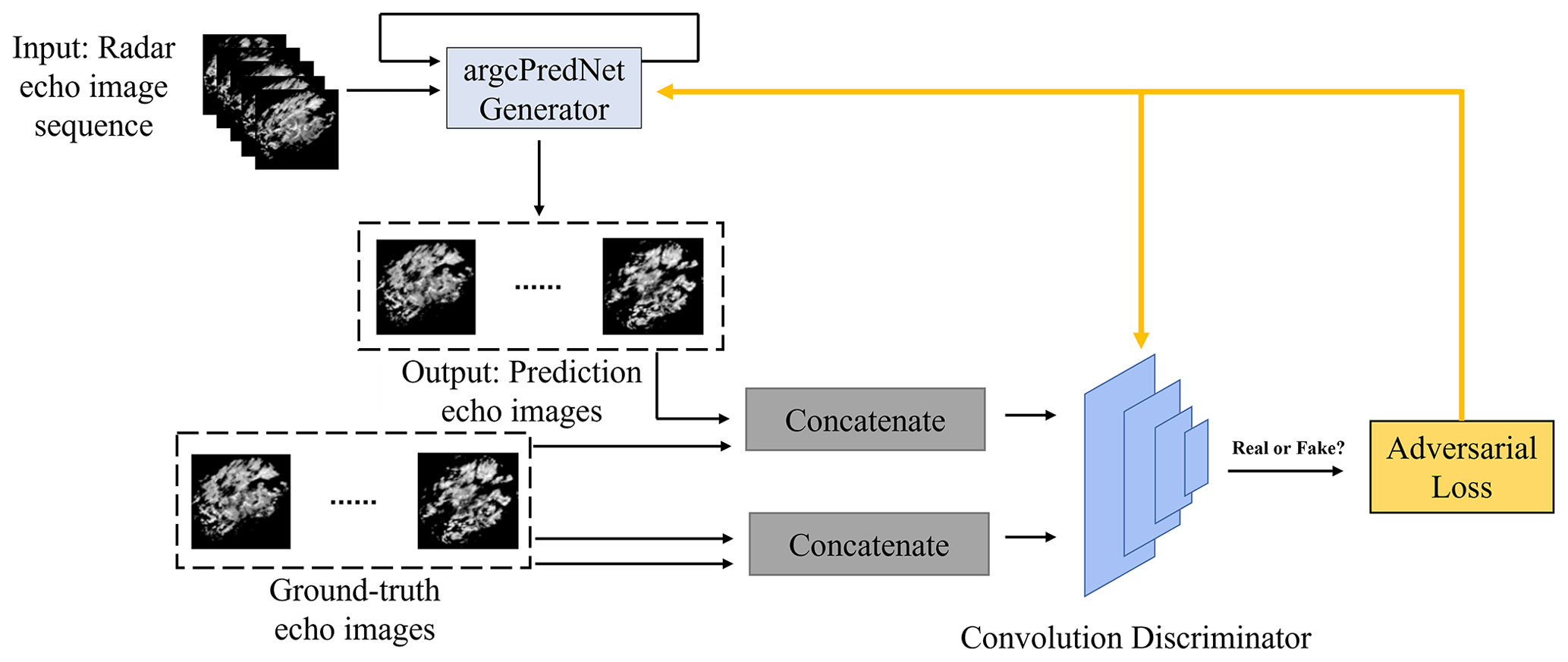
Figure 1The structure of GAN-argcPredNet v1.0. More information about the model can be found in the paper of Zheng et al. (2022).
2.2 GAN-argcPredNet v2.0 overview
The GAN-argcPredNet v2.0 model was built based on GAN-argcPredNet v1.0. GAN-argcPredNet v2.0 consists of a STIC prediction generator and a CS convolution discriminator (Fig. 2). The STIC prediction generator is designed to reduce echo attenuation and consists of the argcPredNet and the STIC attention module (Fig. 3). The argcPredNet is composed of a series of repeatedly stacked modules, with a total of four layers (Zheng et al., 2022). Each layer of the module consists of the input convolutional layer (Al), the recurrent representation layer (Rl), the prediction convolutional layer () and the error representation layer (El). Rl learns image features and generates the feature map , where l, T, H, W and C denote layer, current prediction time, map height, map width and feature channel, respectively. The feature map guides the lower layers to generate images. STIC attention is designed to focus on the importance of different rainfall regions after the third layer. The purpose is to better maintain spatiotemporal features during information transmission within the model. After passing through STIC attention, the features are fed to the lower layers, aiming to avoid blurring or to maintain the intensity during extrapolation. The calculation method of STIC prediction is
Here, xT denotes the initial input, MAXPOOL denotes the maximum pooling operation, γ denotes ReLU activation function, f denotes the convolution operation, argcLSTM denotes advanced reduced-gate convolutional LSTM (Zheng et al., 2022) and STIC denotes STIC attention.
The CS convolution discriminator is composed of a four-layer convolution structure and a CS attention module. The convolution structure is responsible for extracting the echo features from the input radar echo images. CS attention is embedded after the first-layer convolution structure. This module is designed to focus on radar echo features, especially heavy rainfall features. The purpose is to enhance discriminative ability and provide better guidance for the generator. The hyperparameters of the generator and discriminator are provided in the Supplement (Tables S7 and S8).
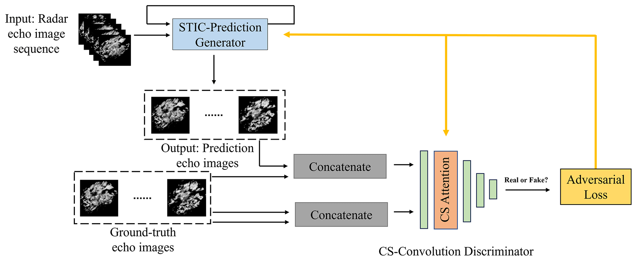
Figure 2The structure of GAN-argcPredNet v2.0. A total of 15 radar echo images are used as a test sequence. Here, the first five images are used as the input sequence, and the last 10 images are used as the ground truth images. The generator generates images based on input sequences. The discriminator judges both the predictive images and ground truth images. The adversarial loss is then obtained to optimize the model.
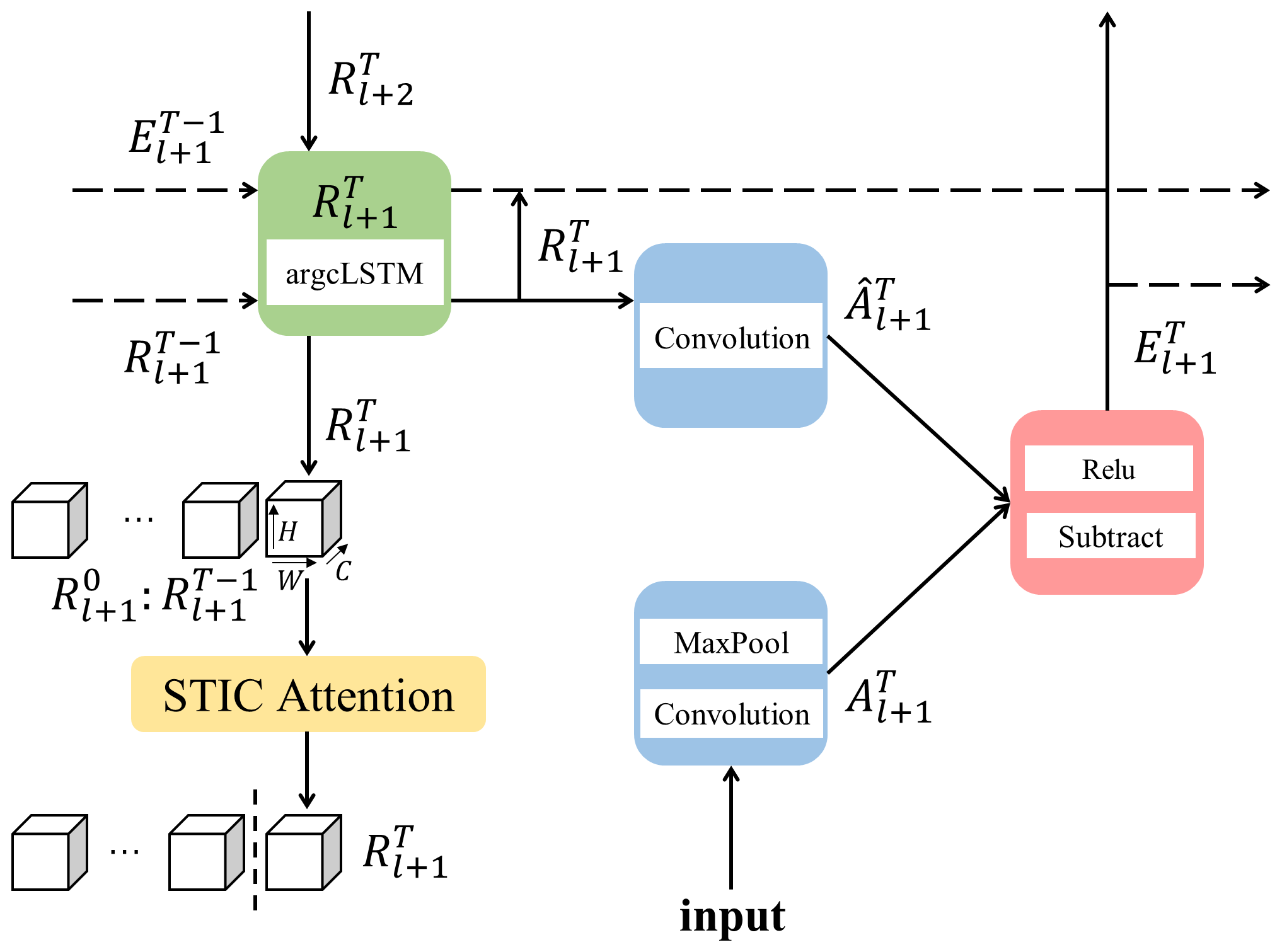
Figure 3The STIC prediction structure at time T with four layers (). The STIC attention is located between the second layer (l=1) and the third layer (l=2). During prediction, forms the sequence with Rl+1 prior to the moment T. Then, the sequence is fed into the STIC module, which captures the correlation between the sequences and adjusts . Finally, the new is output. See Sect. 2.2 for further explanation.
2.3 STIC attention
STIC attention (Fig. 4) combines MaxPool3D (3D is equal to map height, map width and time) and AvgPool3D to focus on the spatial information in feature sequences from both the maximum and average perspectives. This step focuses on heavy rainfall echoes while considering non-heavy rainfall. The introduction of 3D convolution enables extraction of spatiotemporal changes in the feature sequences. The module calculates the importance of evolutionary information. The detailed steps are below.
Given the feature sequence as input, where t denotes time, two feature sequences and are obtained by pooling operations, which denote the maximum and average feature along the channel axis, respectively. The feature sequences are then connected and 3D-convoluted. The activation function is hard_sigmoid. By introducing linear behavior, hard_sigmoid allows gradients to flow easily in the unsaturated state and provides a crisp decision in the saturated state, resulting in far less computational expense (Courbariaux et al., 2015; Gulcehre et al., 2016; Nwankpa et al., 2018). Then, the STIC attention map sequence is obtained. Finally, the output feature sequence is calculated by element-wise multiplication of MSTIC and F. In short, the calculation method of STIC attention is
Here, concat denotes the connection operation, MaxPool3D denotes the 3D maximum pooling operation, AvgPool3D denotes the 3D average pooling operation, denotes the 3D convolution operation with a convolution kernel of , σ denotes the hard_sigmoid activation function and ⊗ denotes the element-wise multiplication.
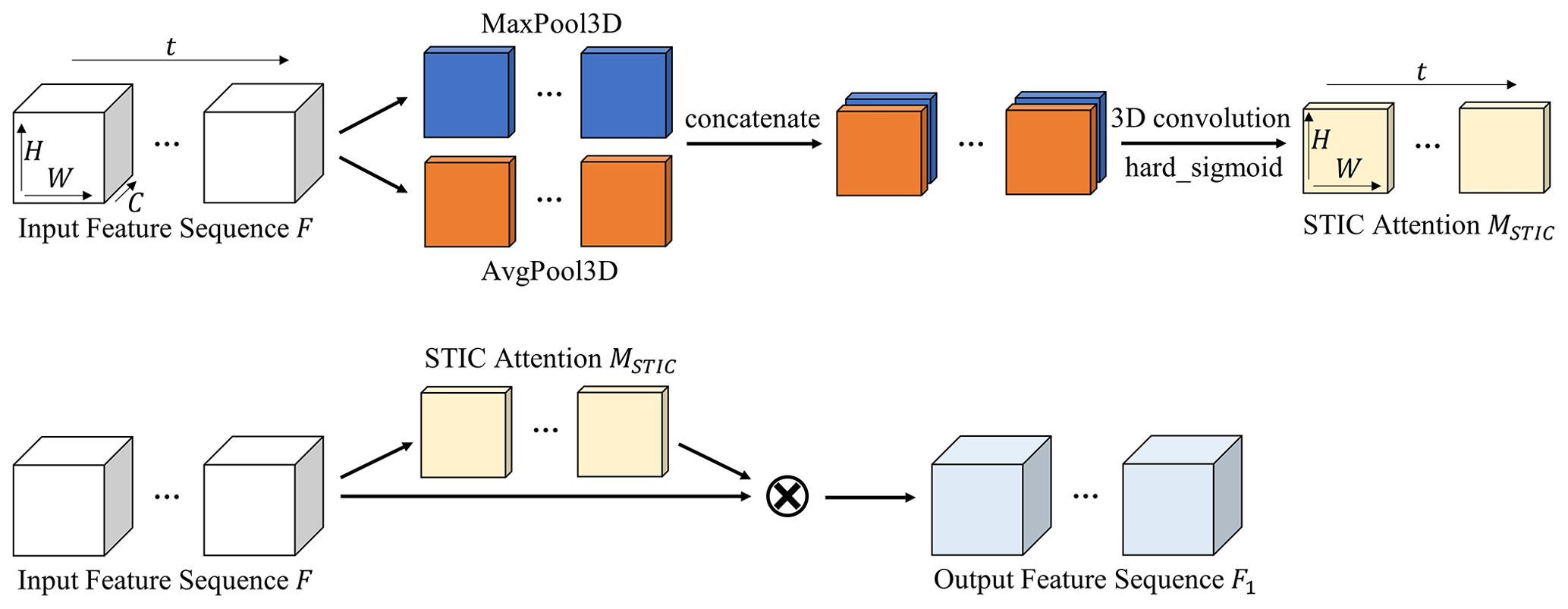
Figure 4The structure of STIC attention. The first line represents the calculation process of the STIC attention map sequence. The second line represents the process of applying the STIC attention map sequence to the input feature sequence.
2.4 CS attention
CS attention consists of channel attention and spatial attention (Fig. 5). For input feature , the channel attention map is first generated. After element-wise multiplication with the initial feature image, the spatial attention map is generated by the spatial attention module. Finally, the output feature is obtained in the same way. In short, the calculation process is as follows:
Here, ⊗ denotes the element-wise multiplication, and is the middle feature.
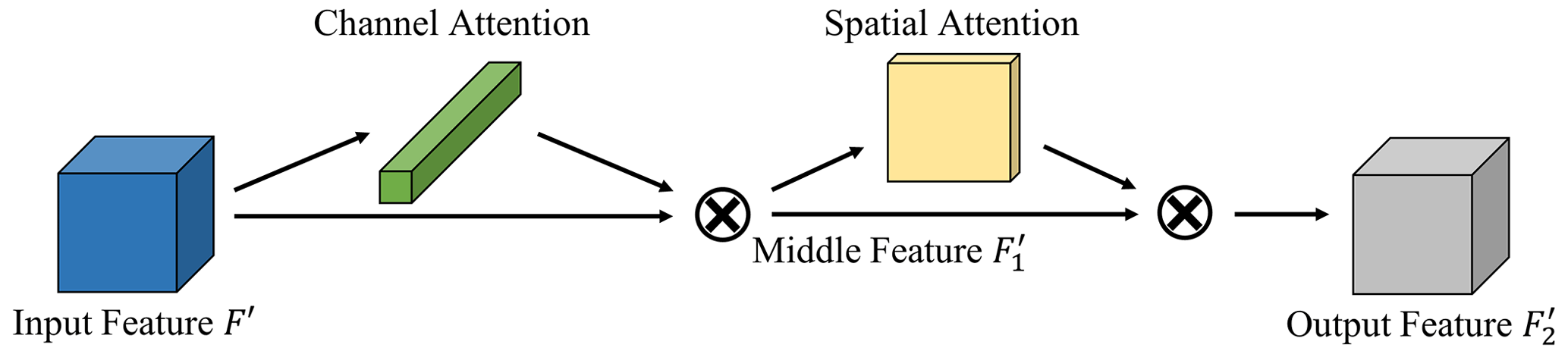
Figure 5The structure of CS attention. The calculation order is first through the channel attention module and then through the spatial attention module.
The channel attention module (Fig. 6) studies the relationship among different feature channels. The global maximum and average pooling is used to gather spatial maximum and average information for each channel. The combination of these methods allows for a more comprehensive judgment of the importance of different feature channels. Then, the correlation between feature channels is obtained by learning the respective parameters in a dense layer. The channel attention module focuses more on meaningful feature channels. The detailed steps are below.
The feature map F′ is input into the channel attention module. Two 1D feature maps and are obtained by applying global pooling, which denote the global maximum and global average pooling features, respectively. Then, the correlation between these features is extracted through dense layers. In order to reduce parameter overhead, the number of neurons in the first dense layer is set to , where r is the compression ratio. Finally, the hard_sigmoid activation function is applied to obtain final channel attention map Mc. In short, the channel attention map is calculated as follows:
Here, GMP denotes the global maximum pooling, GAP denotes the global average pooling, φ10 and φ11 denote the first and second dense layer of , φ20 and φ21 denote the first and second dense layer of , and γ denotes the ReLU activation function.
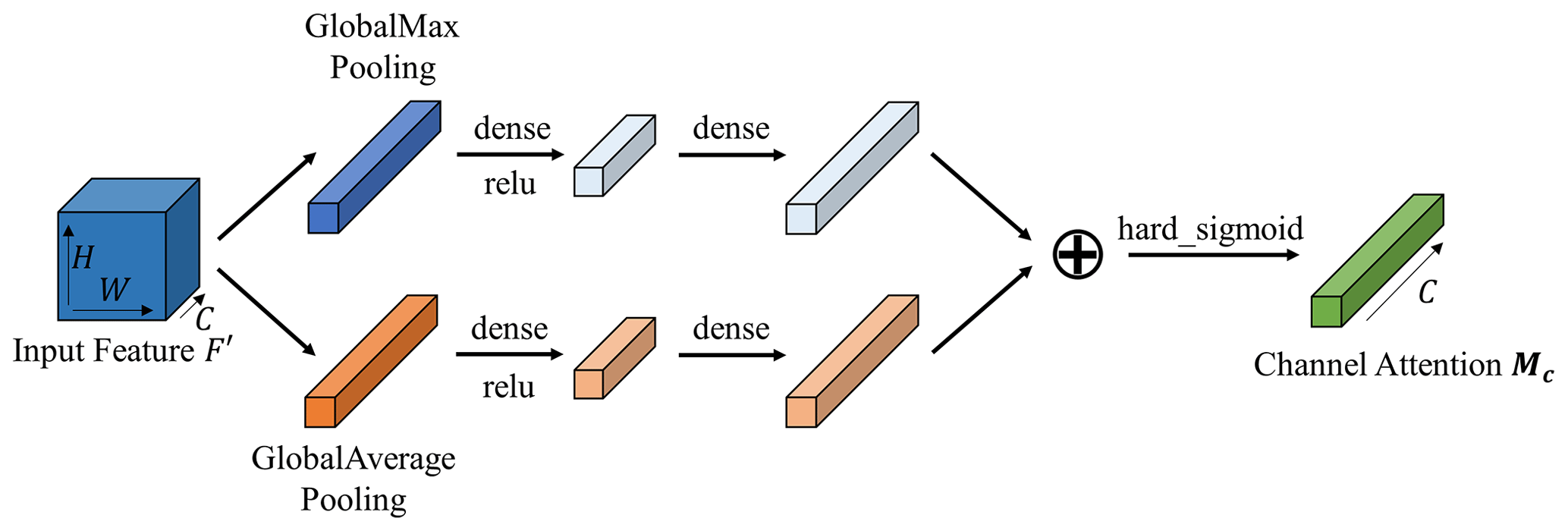
Figure 6The structure of channel attention. Channel attention utilizes maximum pooling outputs and average pooling outputs with their respective networks.
The spatial attention module (Fig. 7) studies the importance of each part in the same channel. The maximum and average pooling is used along the channel axis, which obtains echo information of the feature image. The 2D convolution operation extracts feature and generates a spatial attention map with the same size as the input image. The detailed steps are below.
After the channel attention module, the feature map is input into the spatial attention module. Two 2D feature maps and are obtained by applying pooling operation, which denote the maximum pool feature and average pool feature on the channel, respectively. The feature maps are then connected and 2D-convoluted, using hard_sigmoid as the activation function to obtain final spatial attention map Ms. In short, the calculation method of spatial attention map is
Here, MaxPool2D denotes the 2D maximum pooling operation, AvgPool2D denotes the 2D average pooling operation and f7×7 denotes the 2D convolution operation with a convolution kernel of 7×7.
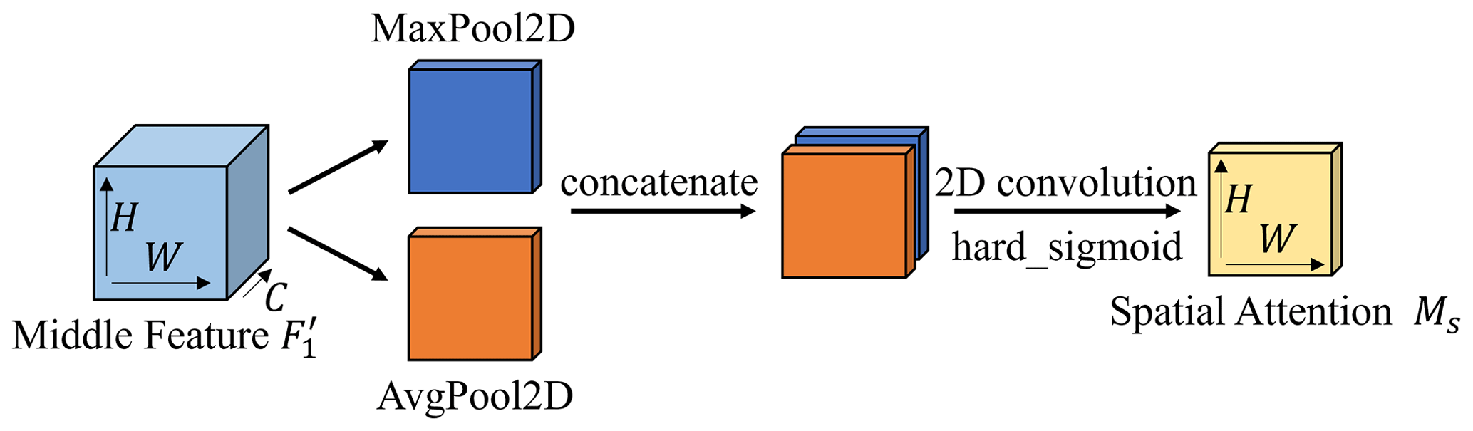
Figure 7The structure of spatial attention. Spatial attention utilizes the maximum and average pooling outputs along the channel axis and forwards them to the convolutional layer.
3.1 Dataset description
This study used the southern China radar echo data provided by Guangzhou Meteorological Bureau. The radar mosaic comes from 11 weather radars. The median filtering algorithm was used to control radar data quality, which eliminates errors caused by isolated clutter. In addition, the mirror filling and continuity checks were applied to remove traditional radar error sources. After quality control, the data contain only an extremely small amount of strong interference, which has a negligible impact on the training of the model.
From 2015 to 2016, a total of 32 010 consecutive echo images with rainfall were randomly selected as the training set. For the testing phase, 7995 consecutive images were randomly selected from March to May 2017. The original resolution of each image is 1050×880 pixels, covering an area of 1050 km × 880 km. Each pixel denotes a resolution of 1 km × 1 km. The reflectivity values range from 0 to 80 dBZ, with the amplitude limit set between 0 and 255. The data, which are the constant-altitude plan position indicator (CAPPI) data, were collected every 6 min at a height of 1 km. To speed up training and reduce hardware load, the central 128 × 128 images were segmented.
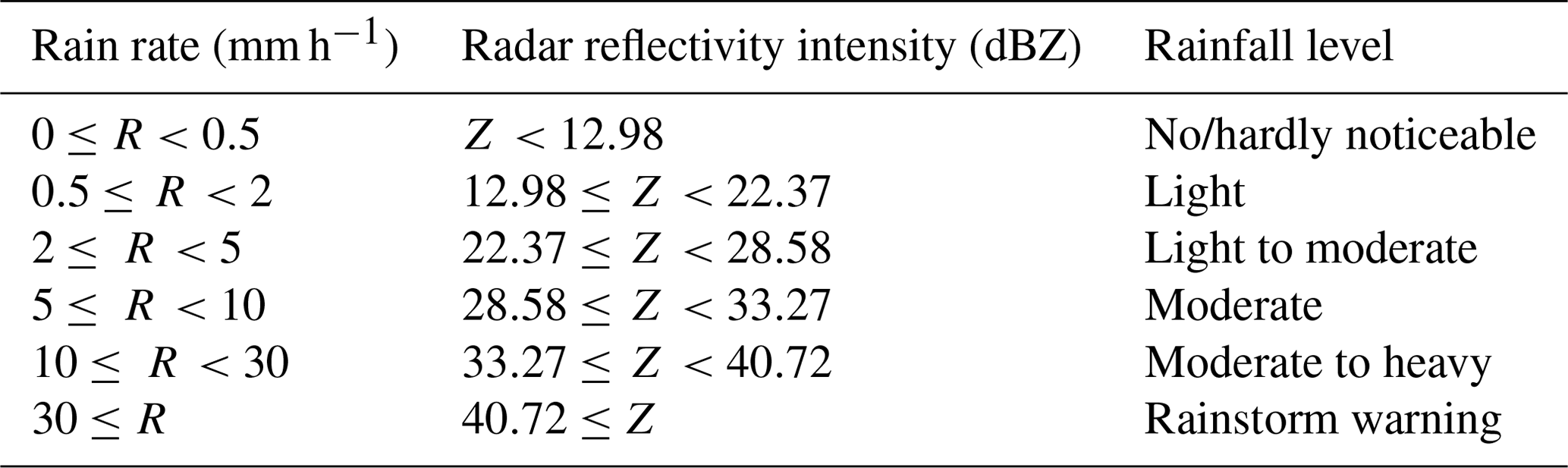
Due to the relationship between radar reflectivity and rainfall type, the value on the radar echo image is converted to the corresponding rainfall rate. The calculation formula is as follows:
Here, a is set to 58.53, b is set to 1.56, Z denotes the radar reflectivity intensity and R denotes the rainfall intensity. The correspondence between rainfall rate, radar reflectivity intensity and rainfall level is referred to in Table 1 (Shi et al., 2017).
Table 1The rainfall level table. Rain rate, radar reflectivity intensity and rainfall level correspond to each other.
3.2 Evaluation metrics
As for evaluation, the study used four metrics to evaluate the prediction accuracy of all 128 × 128 pixels, which are probability of detection (POD), false alarm ratio (FAR), critical success index (CSI) and Heidke skill score (HSS). POD evaluates hit ability, while FAR is the metric of false alarms. The combination of them can evaluate the model more objectively. CSI and HSS are composite metrics that provide a direct judgment of the model effectiveness. CSI measures the fraction of observed and/or forecast events that are correctly predicted. HSS measures the fraction of correct forecasts after eliminating those forecasts which would be correct due purely to random chance. To measure the blurring effect, the study also used the bias score, which evaluates the ratio between the frequency of forecast events and the frequency of observed events. The formulas for calculating these five metrics are as follows:
Here, TP denotes that the real and predicted values reach specified threshold, FN denotes that the real value reaches the specified threshold and the predicted value does not reach, FP denotes that the real value does not reach the specified threshold and the predicted value reaches, and TN denotes that the real value and predicted value do not reach the specified threshold. In the study, we applied threshold rain rates of 0.5, 2, 5, 10 and 30 mm h−1 for calculating these metrics.
In order to evaluate the quality of generated images objectively, mean square error (MSE) and mean structural similarity (MSSIM) were also chosen for the experiment (Wang et al., 2004; Inoue and Misumi, 2022).
3.3 Experimental setting
Radar echo extrapolation is the prediction of future radar echo images based on real images. This study set the input sequence M and output sequence N to 5 and 10, respectively.
GAN-argcPredNet v2.0 was first compared with the optical flow, ConvLSTM, ConvGRU, GA-ConvGRU and GAN-argcPredNet v1.0 in comparison experiments. The first one is a traditional method, and the code comes from the pySTEPS library (Pulkkinen et al., 2019), which we performed using a local tracking approach (Lucas-Kanade). The last one is the model we designed before. Other models are commonly used deep learning models in radar echo extrapolation. The hyperparameters for deep learning models were provided in the Supplement (Tables S1–S6). Then the ablation study was designed to verify the effectiveness of STIC attention and CS attention.
Before training, each pixel of the radar echo image was normalized to [0, 1]. All experiments were implemented by Python. Model training and testing were performed using the Keras deep learning library with TensorFlow as the backend. The operating environment was a Linux workstation equipped with two NVIDIA RTX 2080 Ti 11G GPUs.
4.1 Comparison study
In order to observe the performance of the models and evaluate the blurring effect more easily, the average scores of POD, FAR, CSI, HSS and bias were calculated for 30 and 60 min lead time in the experiment. Figure 8 shows the average scores of the metrics used for predicting 30 min, and the scores of GAN-argcPredNet v2.0 are better than the other models except bias score, especially the thresholds 10 and 30 mm h−1, which indicates that GAN-argcPredNet v2.0 has a significant advantage in forecasting heavy precipitation. In bias score, GAN-argcPredNet v2.0 is second only to the optical flow and better than other deep learning models. The optical flow extrapolates the echo motion as linear, which is not realistic and leads to poorer forecasts. Figure 9 shows the average scores of the metrics used for predicting 60 min. Except for the bias score, most deep learning models have better scores than the optical flow. Besides the threshold of 30 mm h−1, the bias score of the optical flow is second only to GAN-argcPredNet v2.0. In deep learning models, the FAR score of GAN-argcPredNet v2.0 is slightly higher than those of ConvGRU and ConvLSTM at thresholds of 0.5 and 2 mm h−1, respectively. However, the other scores of GAN-argcPredNet v2.0 are always the best. The comprehensive score of GAN-argcPredNet v1.0 is second only to GAN-argcPredNet v2.0. GA-ConvGRU performs better than the two non-GAN models in most cases. Between the two non-GAN models, all scores of ConvLSTM are better than ConvGRU when the threshold is set to 5 and 10 mm h−1.
GAN-argcPredNet v2.0 shows excellent performance in heavy rainfall prediction. During 60 min of forecasting, compared to the baseline GAN-argcPredNet v1.0, the POD, CSI, HSS and bias scores of GAN-argcPredNet v2.0 increase by 20.1 %, 16.0 %, 15.4 % and 25.0 % when the threshold is set to 10 mm h−1. The FAR score also decreases by 2.3 %. When the threshold is set to 30 mm h−1, the POD, CSI, HSS and bias scores increase by 18.8 %, 17.0 %, 17.2 % and 26.3 %, respectively. The FAR score decreases by 3.0 %.
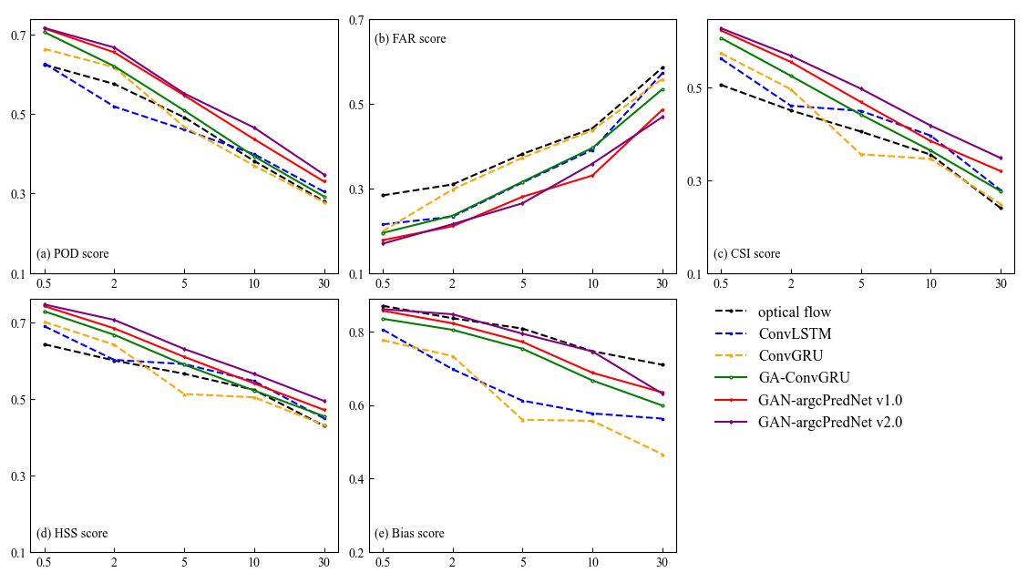
Figure 8The average scores of (a) POD, (b) FAR, (c) CSI, (d) HSS and (e) bias under different thresholds for forecasting 30 min. All the time steps were used to compute the scores. The horizontal axis represents the threshold in units of mm h−1. The perfect score of FAR is 0, while the others are 1.
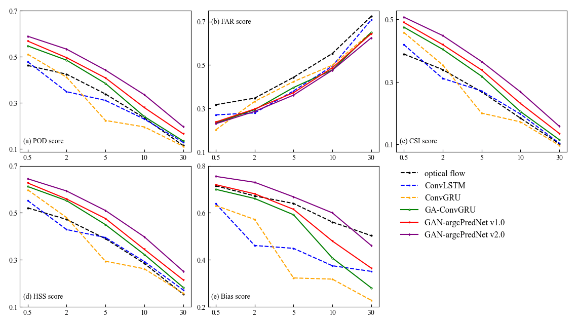
Figure 9The average scores of (a) POD, (b) FAR, (c) CSI, (d) HSS and (e) bias under different thresholds for forecasting 60 min. All the time steps were used to compute the scores. The horizontal axis represents the threshold in units of mm h−1. The perfect score of FAR is 0, while the others are 1.
The experiment selected three prediction examples and drew the extrapolation comparison images and metric scores (Figs. 10–13). In Figs. 10, 11 and 12, in the 0–30 min predictions, the optical flow has an advantage in terms of less change in echo strength and echo shape preservation. However, in regions where there are echoes with rapid change, such as the center region of Fig. 10 and the upper-left region of Figs. 11 and 12, the optical flow overestimates the strength of the echoes, especially the strong echoes. In Fig. 11, the optical flow incorrectly estimates the location of the strong echoes as the storm grows rapidly. Figure 12 shows that the optical flow overestimates the intensity and distorts the predicted echo shape. In contrast, the deep learning model predicted the changes in the echoes, while GAN-argcPredNet v2.0 better preserved the shape of the echoes. In 30–60 min of prediction, all images predicted by the deep learning models showed echo decay. The GAN-argcPredNet v2.0 decayed significantly slower. The intensity and shape of the strong echoes are well maintained in the circular or rectangular labeled areas in the figure, and the prediction results are more consistent with the ground truth. Overall, compared with other methods, GAN-argcPredNet v2.0 can provide more accurate predictions, showing its stronger prediction ability. Figure 13 shows the metric scores at 60 min of forecasting under the 30 mm h−1 threshold for three selected prediction examples. As the prediction time increases, the change curve of GAN-argcPredNet v2.0 is the smoothest, and the long-range curve remains relatively stable, which further verifies the excellent performance of GAN-argcPredNet v2.0 in forecasting heavy rainfall. Specifically, GAN-argcPredNet v2.0 has the best performance in POD, FAR, CSI and HSS curves, and the bias score is only second to the optical flow. Notably, the POD, CSI, HSS and bias scores of ConvGRU and ConvLSTM rapidly drop to 0, and the FAR score rapidly rises to 1, which indicates that the blurring effect seriously affects the performance of heavy rainfall prediction.
The optical flow method consistently exhibits overestimation or misestimation in these examples. In deep learning models, the three GAN-based models also present better echo structure and prediction performance compared to the two non-GAN models. For the echo above 40 dBZ, ConvLSTM exhibits the most severe attenuation. This suggests that echo attenuation and prediction blurring seriously affect the performance of precipitation prediction, especially heavy precipitation.
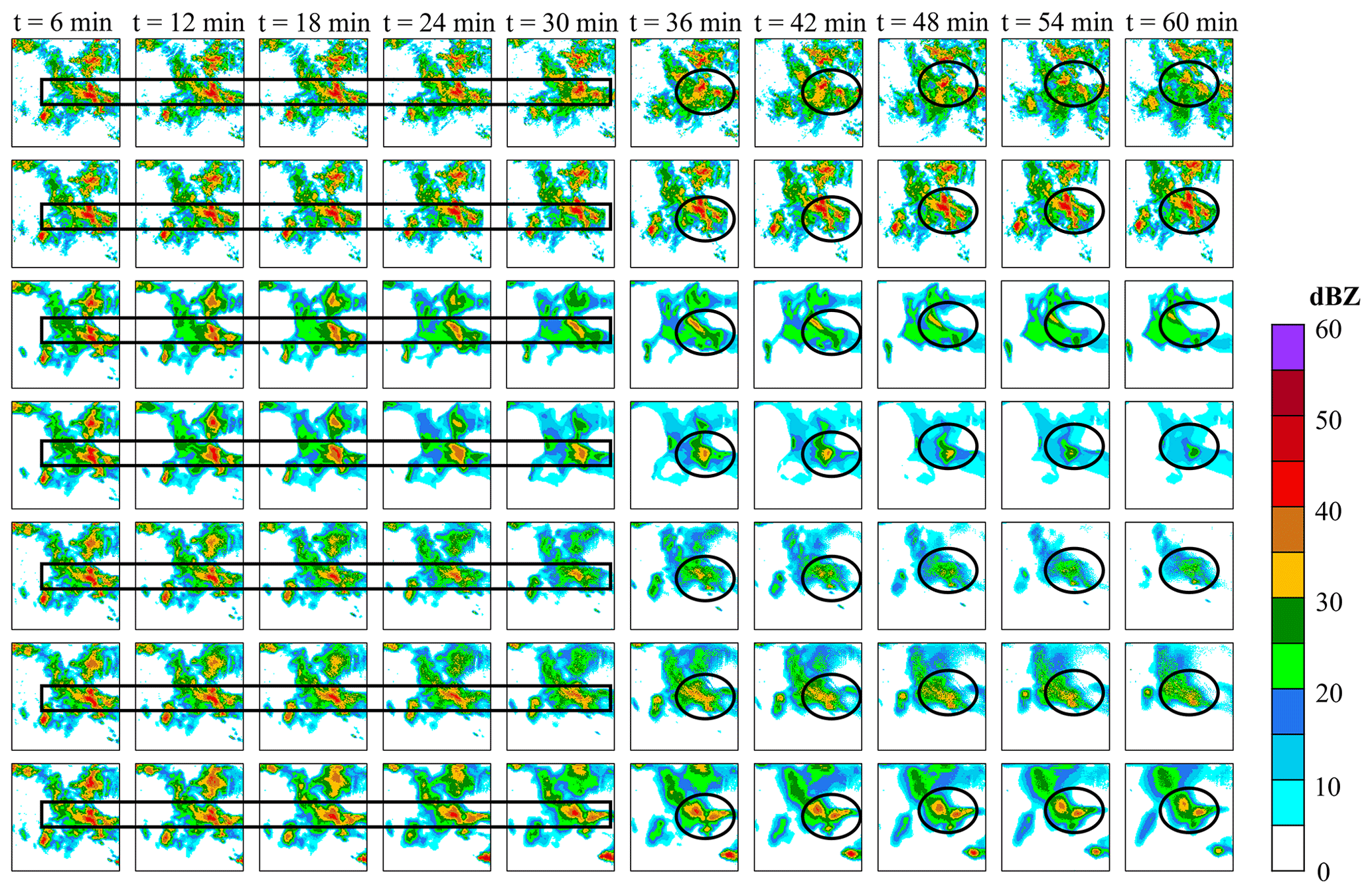
Figure 10The example of the growth of a weather system in radar echo extrapolation. From top to bottom are ground truth frames, prediction by the optical flow, prediction by ConvGRU, prediction by ConvLSTM, prediction by GA-ConvGRU, prediction by GAN-argcPredNet v1.0 and prediction by GAN-argcPredNet v2.0. The circular and rectangular regions represent heavy rainfall prediction, where the performance of the models in extrapolating heavy rainfall can be observed.
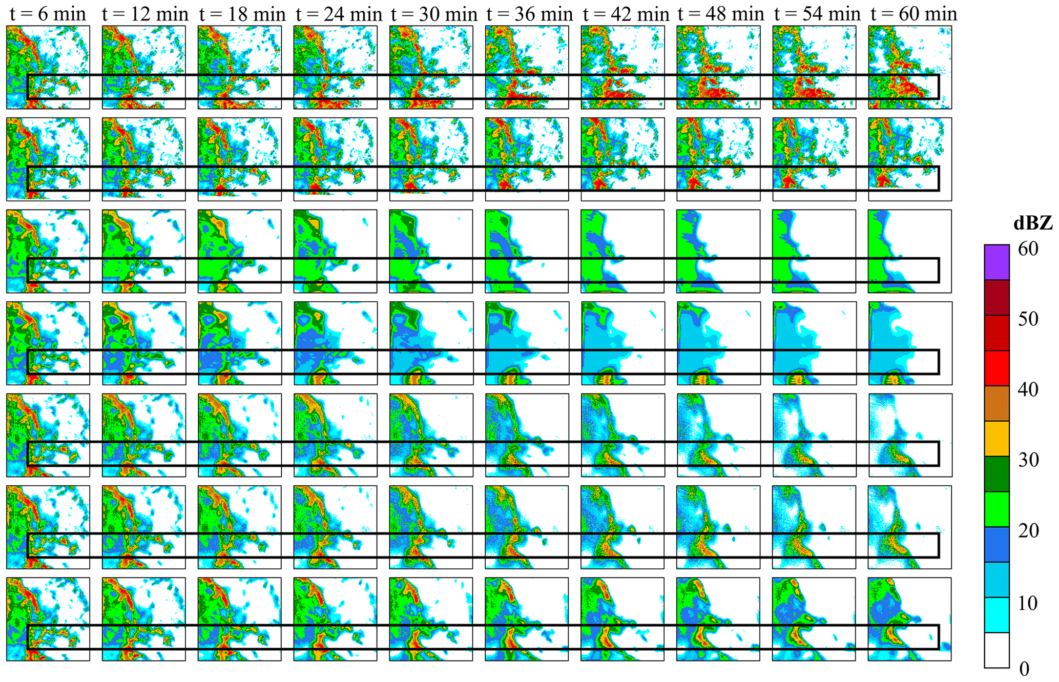
Figure 11The example of rapid storm growth in radar echo extrapolation. From top to bottom are ground truth frames, prediction by the optical flow, prediction by ConvGRU, prediction by ConvLSTM, prediction by GA-ConvGRU, prediction by GAN-argcPredNet v1.0 and prediction by GAN-argcPredNet v2.0. The rectangular region represents the prediction for rapid storm growth.
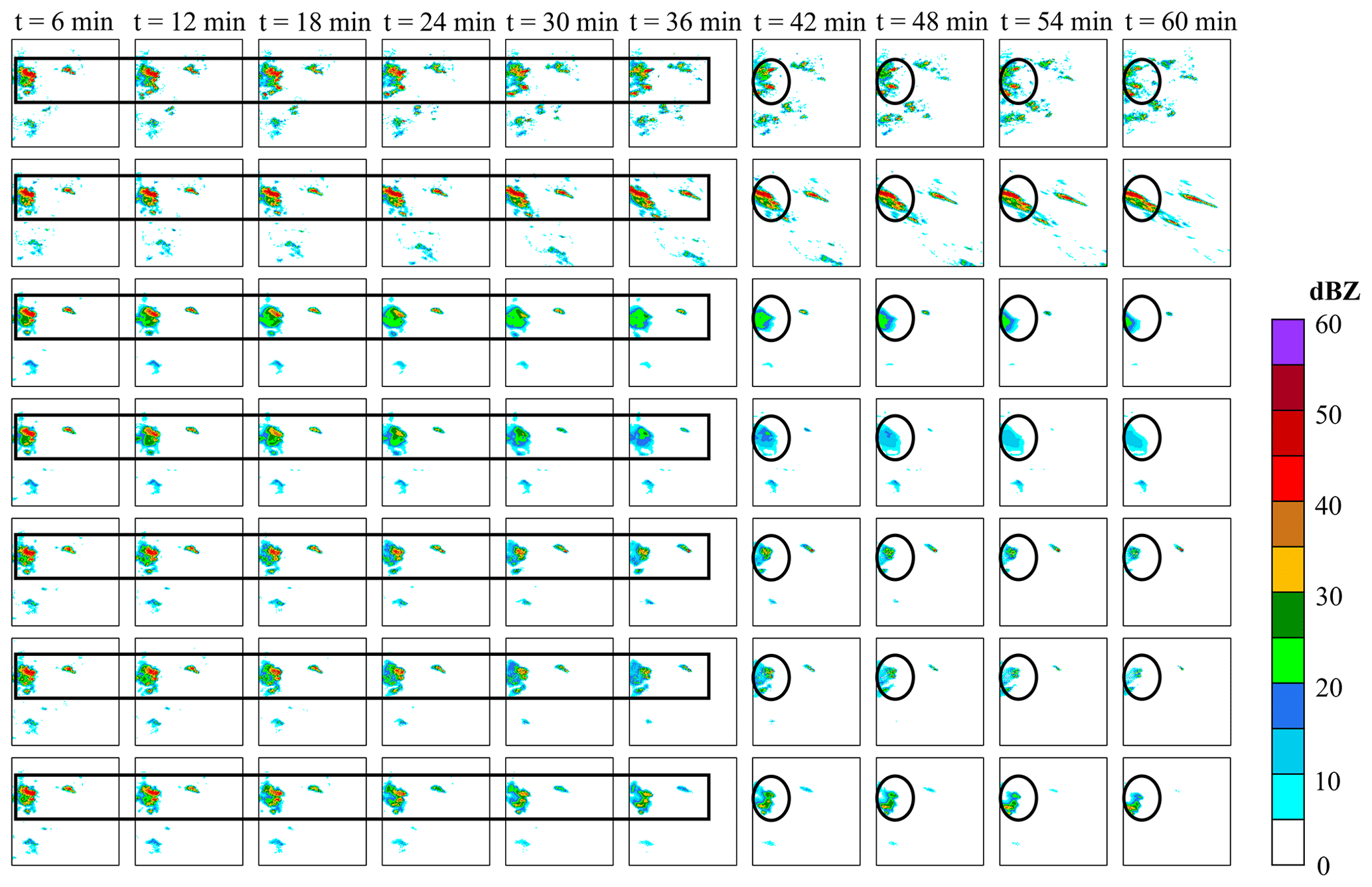
Figure 12The example of storm decay in radar echo extrapolation. From top to bottom are ground truth frames, prediction by the optical flow, prediction by ConvGRU, prediction by ConvLSTM, prediction by GA-ConvGRU, prediction by GAN-argcPredNet v1.0 and prediction by GAN-argcPredNet v2.0. The circular and rectangular regions represent heavy rainfall prediction.
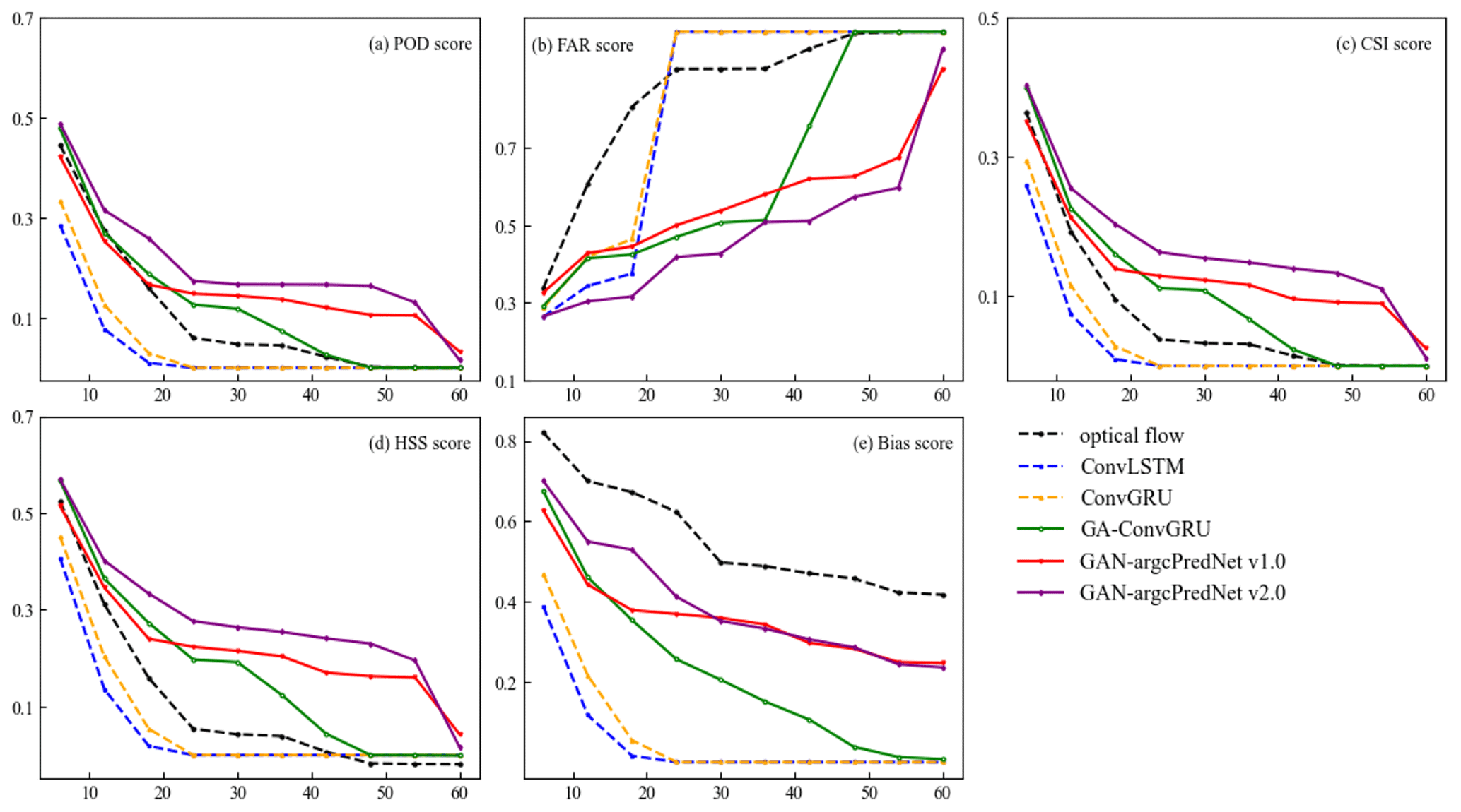
Figure 13The curves of change in (a) POD, (b) FAR, (c) CSI, (d) HSS and (e) bias scores under the threshold of 30 mm h−1 for three selected prediction examples at 60 min of forecasting. The horizontal axis represents the time in units of minutes. The perfect score of FAR is 0, while the others are 1.
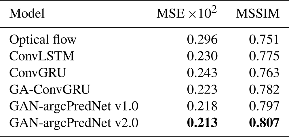
To evaluate the quality of generated images objectively, the experiment also calculated the MSE and MSSIM metrics. Table 2 shows that the optical flow method has the worst score. In deep learning models, GAN-based models have better scores in both MSE and MSSIM, with GAN-argcPredNet v2.0 achieving the best score. Compared to GAN-argcPredNet v1.0, the MSE metric of GAN-argcPredNet v2.0 decreases by 2.3 %, while the MSSIM metric increases by 1.25 %. In the non-GAN models, ConvLSTM scores better.
Table 2The MSE and MSSIM scores of each model. The perfect score of MSE is 0, while the perfect score for MSSIM is 1. Bold represents the best score.
4.2 Ablation study
In the ablation study, we investigated the effects of STIC attention and CS attention. STIC-GAN and CS-GAN were constructed by adding the STIC attention module only in the generator and the CS attention module only in the discriminator. To precisely observe the score differences, the experiment recorded the average score of each metric in a tabular format. Table 3 shows that both CS-GAN and STIC-GAN have better scores than GAN-argcPredNet v1.0. At the threshold of 0.5 mm h−1, CS-GAN achieves the best score in the FAR metric, but other metrics still perform worse than GAN-argcPredNet v2.0. At thresholds of 5, 10 and 30 mm h−1, the metric scores of STIC-GAN exceed those of CS-GAN, which is closer to GAN-argcPredNet v2.0.
Table 3The average scores of POD, FAR, CSI, HSS and bias under different thresholds. All the time steps were used to compute the scores. Bold represents the best score.
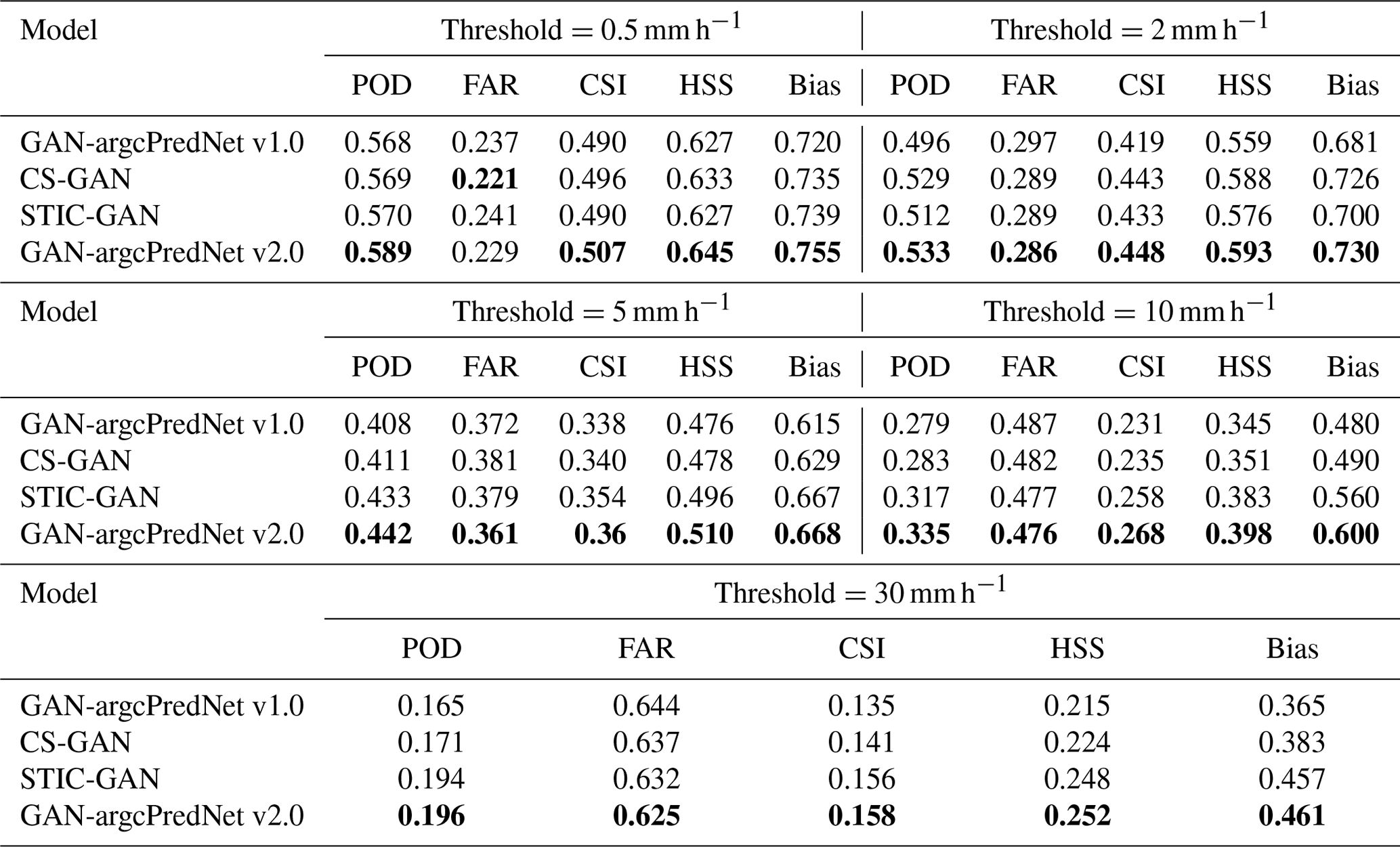
Figure 14 shows that CS-GAN and STIC-GAN retain better echo intensity and shape compared to GAN-argcPredNet v1.0. For heavy rainfall, STIC-GAN shows better prediction with echoes that are closer to GAN-argcPredNet v2.0. In rectangular regions, STIC-GAN accurately predicts rainfall events until 30 min. However, in the circular regions, STIC-GAN overestimates the echo intensity compared to GAN-argcPredNet v2.0.
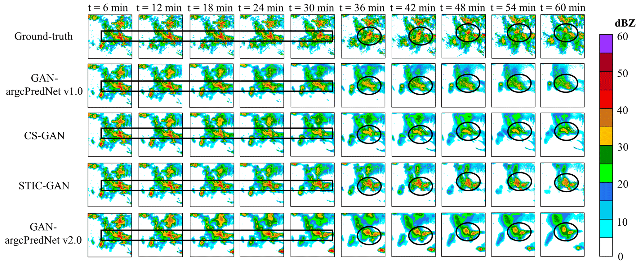
Figure 14The example of radar echo extrapolation. From top to bottom are ground truth frames, prediction by GAN-argcPredNet v1.0, prediction by CS-GAN, prediction by STIC-GAN and prediction by GAN-argcPredNet v2.0. The circular and rectangular regions represent heavy rainfall prediction.
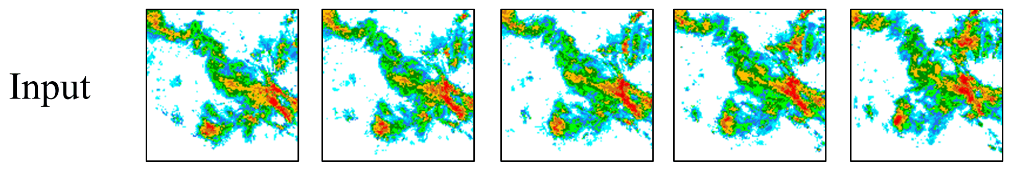
Figure 15The input radar image sequence. The example in Fig. 10 is extrapolated based on these five images.
5.1 Discussion
In the comparison study, the bias score of the optical flow is second only to GAN-argcPredNet v2.0. The result proves that, compared to other deep learning models, the number of rainfall events predicted by the optical flow method is closer to real rainfall events. However, the poor FAR score indicates that there are many false predictions among these predicted events. Considering other metrics as well, most deep learning models perform better than the optical flow method (Figs. 8–9 and Table 2). In deep learning models, the three GAN-based models have higher prediction accuracy and better image quality compared to the two non-GAN models. This indicates that GAN structure has more advantages with its powerful image generation capability. Although ConvLSTM and ConvGRU sometimes have lower FAR scores, according to metrics such as POD, this is due to the fact that they fail to predict a large number of rainfall events. As the number of predicted rainfall events decreases, the false alarm rate also decreases. Combined with the bias score, ConvLSTM and ConvGRU generally predict a lower frequency of rainfall than other models. This indicates that they suffer from a more severe blurring effect. GA-ConvGRU and GAN-argcPredNet v1.0 improve the prediction accuracy with GAN structure, but the phenomenon of echo attenuation also cannot be ignored.
GAN-argcPredNet v2.0 achieves the highest prediction accuracy and quality, suggesting its effectiveness in curbing echo attenuation compared to other models. This is because the echo intensity and shape are better maintained by suppressing the blurring effect of rain distribution and reducing the negative bias. According to the scores at the thresholds of 10 and 30 mm h−1, it can be observed that GAN-argcPredNet v2.0 exhibits the best improvement in predicting heavy rainfall.
GAN-argcPredNet v2.0 maintains the evolution trend well, but there are still some special cases (Fig. 10). There are some false predictions on the bottom-right corner, and the rain area near the top right goes out of the domain. This is because in the input sequence (Fig. 15), the rainfall on the bottom-right corner shows a growing trend, and the rain area near the top right shows a trend of moving towards the upper left. Our model retains the information and maintains the trend through the attention mechanism, but there are still some deviations from ground truth. This may be overcome by increasing the dataset and strengthening training on special cases. Also, the strong echoes outside the center of the echo images are not as well represented as the main features during the extrapolation. This is because in the input sequence, the other strong echoes have a smaller spatial range, making them more susceptible to attenuation during extrapolation. In Figs. 10–11, GAN-argcPredNet v2.0 has a clear advantage for out-of-center regions in curbing the attenuation compared to other deep learning models, and there are fewer incorrect predictions compared to the optical flow. This indicates that GAN-argcPredNet v2.0 focuses on the main features and also pays more attention to the minor features with rapid growth than other models. Overall, GAN-argcPredNet v2.0 is capable of curbing echo attenuation, the center region is more significant and the overall performance is more competitive.
In the ablation study, we find that the scores of CS-GAN and STIC-GAN are mostly better than GAN-argcPredNet v1.0 (Table 3 and Fig. 14). This indicates that both STIC attention and CS attention can curb echo attenuation and improve prediction accuracy. As the threshold increases, the scores of STIC-GAN become closer to that of GAN-argcPredNet v2.0. This is because STIC attention focuses more on the rapidly evolving areas of the radar images. CS attention helps GAN-argcPredNet v2.0 achieve better overall performance.
5.2 Conclusions
The study improves precipitation nowcasting by reducing echo attenuation. By avoiding blurring or maintaining the intensity, GAN-argcPredNet v2.0 curbs the attenuation and improves the rainfall prediction accuracy, especially for heavy rainfall. STIC attention suppresses the blurring effect of rain distribution and reduces the negative bias, allowing the generator to generate more accurate images. CS attention enables the discriminator to better guide the generator to maintain echo intensity and shape. Meanwhile, the model is designed based on the generative adversarial structure, which achieves high-quality radar echo extrapolation.
In practice, predictive software has been developed based on our model. After the software accesses the radar data and establishes a prediction task, rainfall prediction results are output as a dataset. Then the dataset can be fed into the urban flood warning system. The improvement of rainfall prediction has a positive impact on flood prediction and urban operation safety.
Overall, GAN-argcPredNet v2.0 is a spatiotemporal process enhancement model based on GAN, which achieves more accurate rainfall prediction.
Future work can be considered from two aspects. The prediction accuracy of the model proposed in the study still has room for improvement. Given the proven efficacy of data assimilation in numerous fields, exploring the integration of data assimilation techniques with other meteorological variables, such as temperature, to study multi-modal models represents a crucial direction for precipitation nowcasting. High-resolution prediction is often limited by hardware, such as a graphics card. Therefore, it is possible to reduce the need for hardware by optimizing the algorithm complexity and the number of parameters.
The radar data used in the paper come from Guangdong Meteorological Bureau. Due to the confidentiality policy, we only provide a sequence of 12 images. If you need to access more data, please contact Kun Zheng (zhengk@cug.edu.cn) and Qiya Tan (ses_tqy@cug.edu.cn). The GAN-argcPredNet v2.0 model is open source. You can find the source code from https://doi.org/10.5281/zenodo.7505030 (Tan, 2022).
Tables S1–8 are provided in Supplement. The supplement related to this article is available online at: https://doi.org/10.5194/gmd-17-399-2024-supplement.
KZ and QT were responsible for developing models and writing the paper; HR, JZ, CL, ST, YY, YT and JC were responsible for data screening and preprocessing.
The contact author has declared that none of the authors has any competing interests.
Publisher's note: Copernicus Publications remains neutral with regard to jurisdictional claims made in the text, published maps, institutional affiliations, or any other geographical representation in this paper. While Copernicus Publications makes every effort to include appropriate place names, the final responsibility lies with the authors.
This research has been supported by the Science and Technology Planning Project of Guangdong Province (grant no. 2018B020207012).
This paper was edited by Shu-Chih Yang and reviewed by three anonymous referees.
Austin, G. and Bellon, A.: The use of digital weather radar records for short-term precipitation forecasting, Q. J. Roy. Meteor. Soc., 100, 658–664, 1974.
Ayzel, G., Scheffer, T., and Heistermann, M.: RainNet v1.0: a convolutional neural network for radar-based precipitation nowcasting, Geosci. Model Dev., 13, 2631–2644, https://doi.org/10.5194/gmd-13-2631-2020, 2020.
Ballas, N., Yao, L., Pal, C., and Courville, A.: Delving deeper into convolutional networks for learning video representations, arXiv [preprint], https://doi.org/10.48550/arXiv.1511.06432, 2015.
Bowler, N. E., Pierce, C. E., and Seed, A.: Development of a precipitation nowcasting algorithm based upon optical flow techniques, J. Hydrol., 288, 74–91, https://doi.org/10.1016/j.jhydrol.2003.11.011, 2004.
Chen, H. G., Zhang, X., Liu, Y. T., and Zeng, Q. Y.: Generative Adversarial Networks Capabilities for Super-Resolution Reconstruction of Weather Radar Echo Images, Atmosphere, 10, 555, https://doi.org/10.3390/atmos10090555, 2019.
Chung, K.-S. and Yao, I.-A.: Improving radar echo Lagrangian extrapolation nowcasting by blending numerical model wind information: Statistical performance of 16 typhoon cases, Mon. Weather Rev., 148, 1099–1120, 2020.
Courbariaux, M., Bengio, Y., and David, J. P.: Binaryconnect: Training deep neural networks with binary weights during propagations, 28th Annual Conference on Neural Information Processing Systems (NIPS), 9, 3123–3131, https://doi.org/10.5555/2969442.2969588, 2015.
Dixon, M. and Wiener, G.: TITAN: Thunderstorm identification, tracking, analysis, and nowcasting-A radar-based methodology, J. Atmos. Ocean. Tech., 10, 785–797, 1993.
Goodfellow, I., Pouget-Abadie, J., Mirza, M., Xu, B., Warde-Farley, D., Ozair, S., Courville, A., and Bengio, Y.: Generative adversarial networks, Commun. ACM, 63, 139–144, 2020.
Gulcehre, C., Moczulski, M., Denil, M., and Bengio, Y.: Noisy activation functions, 33rd Annual Conference on International Conference on Machine Learning (ICML), 10, 3059–3068, https://doi.org/10.5555/3045390.3045712, 2016.
Gulrajani, I., Ahmed, F., Arjovsky, M., Dumoulin, V., and Courville, A. C.: Improved training of wasserstein gans, 31st Annual Conference on Neural Information Processing Systems (NIPS), 11, 5769–5779, https://doi.org/10.5555/3295222.3295327, 2017.
Han, L., Fu, S. X., Zhao, L. F., Zheng, Y. G., Wang, H. Q., and Lin, Y. J.: 3D Convective Storm Identification, Tracking, and Forecasting-An Enhanced TITAN Algorithm, J. Atmos. Ocean. Tech., 26, 719–732, https://doi.org/10.1175/2008jtecha1084.1, 2009.
Inoue, T. and Misumi, R.: Learning from Precipitation Events in the Wider Domain to Improve the Performance of a Deep Learning-based Precipitation Nowcasting Model, Weather Forecast., 37, 1013–1026, https://doi.org/10.1175/WAF-D-21-0078.1, 2022.
Kingma Diederik, P. and Adam, J. B.: A method for stochastic optimization, arXiv [preprint], https://doi.org/10.48550/arXiv.1412.6980, 2014.
Liu, Y., Xi, D.-G., Li, Z.-L., and Hong, Y.: A new methodology for pixel-quantitative precipitation nowcasting using a pyramid Lucas Kanade optical flow approach, J. Hydrol., 529, 354–364, 2015.
Lotter, W., Kreiman, G., and Cox, D.: Deep predictive coding networks for video prediction and unsupervised learning, arXiv [preprint], https://doi.org/10.48550/arXiv.1605.08104, 2016.
Luo, C., Li, X., and Ye, Y.: PFST-LSTM: A spatiotemporal LSTM model with pseudoflow prediction for precipitation nowcasting, IEEE J. Sel. Top. Appl., 14, 843–857, https://doi.org/10.1109/JSTARS.2020.3040648, 2020.
Luo, C. Y., Li, X. T., Wen, Y. L., Ye, Y. M., and Zhang, X. F.: A Novel LSTM Model with Interaction Dual Attention for Radar Echo Extrapolation, Remote Sens., 13, 164, https://doi.org/10.3390/rs13020164, 2021.
Nerini, D., Foresti, L., Leuenberger, D., Robert, S., and Germann, U.: A reduced-space ensemble Kalman filter approach for flow-dependent integration of radar extrapolation nowcasts and NWP precipitation ensembles, Mon. Weather Rev., 147, 987–1006, 2019.
Nwankpa, C., Ijomah, W., Gachagan, A., and Marshall, S.: Activation functions: Comparison of trends in practice and research for deep learning, arXiv [preprint], https://doi.org/10.48550/arXiv.1811.03378, 2018.
Pan, X., Lu, Y. H., Zhao, K., Huang, H., Wang, M. J., and Chen, H. A.: Improving Nowcasting of Convective Development by Incorporating Polarimetric Radar Variables into a Deep-Learning Model, Geophys. Res. Lett., 48, e2021GL095302, https://doi.org/10.1029/2021gl095302, 2021.
Pulkkinen, S., Nerini, D., Pérez Hortal, A. A., Velasco-Forero, C., Seed, A., Germann, U., and Foresti, L.: Pysteps: an open-source Python library for probabilistic precipitation nowcasting (v1.0), Geosci. Model Dev., 12, 4185–4219, https://doi.org/10.5194/gmd-12-4185-2019, 2019.
Pulkkinen, S., Chandrasekar, V., and Niemi, T.: Lagrangian Integro-Difference Equation Model for Precipitation Nowcasting, J. Atmos. Ocean. Tech., 38, 2125–2145, 2021.
Ravuri, S., Lenc, K., Willson, M., Kangin, D., Lam, R., Mirowski, P., Fitzsimons, M., Athanassiadou, M., Kashem, S., Madge, S., Prudden, R., Mandhane, A., Clark, A., Brock, A., Simonyan, K., Hadsell, R., Robinson, N., Clancy, E., Arribas, A., and Mohamed, S.: Skilful precipitation nowcasting using deep generative models of radar, Nature, 597, 672, https://doi.org/10.1038/s41586-021-03854-z, 2021.
Reyniers, M.: Quantitative Precipitation Forecasts based on radar observations: principles, algorithms and operational systems, Institut Royal Météorologique de Belgique Brussel, Belgium, 1–62, https://orfeo.belnet.be/handle/internal/8780 (last access: 11 January 2024), 2008.
Sakaino, H.: Spatio-Temporal Image Pattern Prediction Method Based on a Physical Model with Time-Varying Optical Flow, IEEE T. Geosci. Remote, 51, 3023–3036, https://doi.org/10.1109/tgrs.2012.2212201, 2013.
Shi, X. J., Chen, Z. R., Wang, H., Yeung, D. Y., Wong, W. K., and Woo, W. C.: Convolutional LSTM Network: A Machine Learning Approach for Precipitation Nowcasting, 29th Annual Conference on Neural Information Processing Systems (NIPS), Montreal, Canada, 9, 802–810, https://doi.org/10.5555/2969239.2969329, 2015.
Shi, X. J., Gao, Z. H., Lausen, L., Wang, H., Yeung, D. Y., Wong, W. K., and Woo, W. C.: Deep Learning for Precipitation Nowcasting: A Benchmark and A New Model, 31st Annual Conference on Neural Information Processing Systems (NIPS), Long Beach, CA, 11, 5622–5632, https://doi.org/10.5555/3295222.3295313, 2017.
Sutskever, I., Vinyals, O., and Le, Q. V.: Sequence to sequence learning with neural networks, 27th Annual Conference on Neural Information Processing Systems (NIPS), Montreal, Canada, 9, 3104–3112, https://doi.org/10.5555/2969033.2969173, 2014.
Tan, Q.: GAN-argcPredNet v2.0, Zenodo [code], https://doi.org/10.5281/zenodo.7505030, 2022.
Tian, L., Li, X. T., Ye, Y. M., Xie, P. F., and Li, Y.: A Generative Adversarial Gated Recurrent Unit Model for Precipitation Nowcasting, IEEE Geosci. Remote Sens. Lett., 17, 601–605, https://doi.org/10.1109/lgrs.2019.2926776, 2020.
Wang, X., Girshick, R., Gupta, A., and He, K.: Non-local neural networks, Proceedings of the IEEE/CVF Conference on Computer Vision and Pattern Recognition (CVPR), Salt Lake City, UT, USA, 7794–7803, https://doi.org/10.1109/CVPR.2018.00813, 2018.
Wang, Y., Jiang, L., Yang, M.-H., Li, L.-J., Long, M., and Fei-Fei, L.: Eidetic 3D LSTM: A model for video prediction and beyond, 7th International Conference on Learning Representations (ICLR), New Orleans, USA, 1–14, https://openreview.net/forum?id=B1lKS2AqtX (last access: 11 January 2024), 2019.
Wang, Z., Bovik, A. C., Sheikh, H. R., and Simoncelli, E. P.: Image quality assessment: from error visibility to structural similarity, IEEE T. Image Process., 13, 600–612, https://doi.org/10.1109/TIP.2003.819861, 2004.
Woo, S., Park, J., Lee, J.-Y., and Kweon, I. S.: bam: Convolutional block attention module, 15th Conference on European conference on computer vision (ECCV), Munich, Germany, 17, 3–19, https://doi.org/10.1007/978-3-030-01234-2_1, 2018.
Xie, P. F., Li, X. T., Ji, X. Y., Chen, X. L., Chen, Y. Z., Liu, J., and Ye, Y. M.: An Energy-Based Generative Adversarial Forecaster for Radar Echo Map Extrapolation, IEEE Geosci. Remote Sens. Lett., 19, 1–5, https://doi.org/10.1109/lgrs.2020.3023950, 2022.
Zheng, K., Liu, Y., Zhang, J., Luo, C., Tang, S., Ruan, H., Tan, Q., Yi, Y., and Ran, X.: GAN–argcPredNet v1.0: a generative adversarial model for radar echo extrapolation based on convolutional recurrent units, Geosci. Model Dev., 15, 1467–1475, https://doi.org/10.5194/gmd-15-1467-2022, 2022.