Quantifying the impact of SST feedback frequency on Madden–Julian oscillation simulations

This study uses the Community Atmosphere Model 5.3 coupled to a 1-D ocean model to investigate the effects of intraseasonal sea surface temperature (SST) feedback frequency on Madden–Julian oscillation (MJO) simulations with intervals at 30 min and 1, 3, 6, 12, 18, 24, and 30 d. The large-scale nature of the MJO in simulations remains intact with decreasing feedback frequency, although it becomes increasingly unrealistic in both structure and amplitude, until 1 per 30 d when the intraseasonal fluctuations are overwhelmingly dominated by unorganized small-scale perturbations in both atmosphere and ocean, as well as at the atmosphere–ocean interface where heat and energy are rigorously exchanged. The main conclusion is that the less frequent the SST feedback, the more unrealistic the simulations. Our results suggest that more spontaneous atmosphere–ocean interaction (e.g., ocean response once every time step to every 3 d in this study) with high vertical resolution in the ocean model is a key to the realistic simulation of the MJO and should be properly implemented in climate models.

1 Introduction

The Madden–Julian oscillation (MJO) is a large-scale tropical circulation that propagates eastward from the tropical Indian Ocean (IO) to the western Pacific (WP) with a periodicity of 30–80 d (Madden and Julian, 1972). In the Indo-Pacific region, the MJO processes involve intraseasonal variability in sea surface temperature (SST) (Chang et al., 2019; DeMott et al., 2014, 2015; Jiang et al., 2015, 2020; Krishnamurti et al., 1988; Li et al., 2014; T. Li et al., 2020; Newman et al., 2009; Pei et al., 2018; Stan, 2018; Tseng et al., 2015). The tropical air–sea interaction, influenced by the upper ocean, plays a crucial role in determining MJO characteristics due to the high heat capacity of the upper ocean within the intraseasonal range, which acts as a significant heat source for atmospheric variability (Watterson, 2002; Sobel and Gildor, 2003; Maloney and Sobel, 2004; Sobel et al., 2010; Liang and Du, 2022).

Analyzing the mechanism of the intraseasonal oscillation (ISO) reveals that heat fluxes play a critical role in the development of intraseasonal SST variability (Hong et al., 2017; Liang et al., 2018). As demonstrated in Fu et al. (2017), underestimation (overestimation) of the air–sea coupling's impact on MJO simulations occurs when it is weak (strong) in the intraseasonal SST variability. Simulation improvements in the eastward propagation and regulation of MJO periodicity in the coupled models can be attributed to several factors such as enhanced low-level convergence and convective instability to the east of convection, as well as enhanced latent heat fluxes (Savarin and Chen, 2022) and SST cooling to the west of convection (DeMott et al., 2014). SST gradients have been found to induce patterns of mass convergence and divergence within the marine boundary layer (MBL), initiating atmospheric convection (de Szoeke and Maloney, 2020; Lambaerts et al., 2020).

Several recent studies have made significant progress in understanding the impact of air–sea coupling on the MJO, particularly at subdaily scales (e.g., DeMott et al., 2015; Kim et al., 2018; Seo et al., 2014; Voldoire et al., 2022; Zhao and Nasuno, 2020). However, there is relatively limited discussion on the effect of air–sea coupling from few days to within half of the MJO period. Several studies have investigated the impact of intraseasonal SST on the MJO by coupled or uncoupled models. (e.g., DeMott et al., 2014; Gao et al., 2020b; Klingaman and Demott, 2020; Pariyar et al., 2023; Stan, 2018). Simulations using time-varying SSTs from coupled global climate model (CGCM) to force the atmospheric general circulation model (AGCM) showed a reduced intraseasonal SST variability, leading to weakened air–sea heat fluxes and eastward propagation (DeMott et al., 2014; Gao et al., 2020b; Klingaman and Demott, 2020; Pariyar et al., 2023). Moreover, the absence of few days variability in SST promotes the amplification of westward power associated with Rossby waves (Stan, 2018).

Incorporating two-way coupling between the ocean and atmosphere has been proved valuable for simulating and predicting intraseasonal variability (e.g., DeMott et al., 2014; Lan et al., 2022; Stan, 2018; Tseng et al., 2015, 2020). As demonstrated in recent studies (e.g., Ge et al., 2017; Lan et al., 2022; Shinoda et al., 2021; Tseng et al., 2015, 2022), incorporating high vertical resolution near the ocean surface positively influences the accurate representation of intraseasonal SST variability and enhances the MJO prediction capabilities. However, how frequent the coupling is needed is still not fully understood, considering the fact that the ocean and atmosphere could evolve in distinct timescales. Also, would the coupling frequency in numerical models influence the accuracy of the MJO simulation?

In this study, we aim to investigate the specific effects of oceanic feedback frequency (FF) through air–sea coupling on the atmospheric intraseasonal variability, using the National Center for Atmospheric Research (NCAR) Community Atmosphere Model 5.3 (CAM5.3) coupled with the single-column ocean model named Snow–Ice–Thermocline (SIT). The coupled model is referred to as CAM5–SIT. The SIT model, consisting of 41 vertical layers, enables the simulation of SST and upper ocean temperature variations with high vertical resolution (Lan et al., 2022). We have demonstrated in previous studies that coupling the SIT significantly improved the MJO simulations in several AGCMs (Tseng et al., 2015, 2022; Lan et al., 2022). The ability of the SIT with extremely high resolutions (i.e., 12 layers within the first 10.5 m) to well resolve the upper ocean warm layer and the cool skin of the ocean surface was identified as the main reason for the improved simulations.

The structure of this paper is organized as follows: Sect. 2 introduces the model, data, methodology, and experiments employed in this study. The performance of the CAM5–SIT models in simulating the MJO is discussed in Sect. 3, while Sect. 4 focuses on the impact of different configurations of subseasonal SST feedback periodicity on MJO simulations. Finally, Sect. 5 presents the conclusions.

2 Data, model experiments, and methodology

2.1 Observational data

Observational datasets used in this study include precipitation from the Global Precipitation Climatology Project (GPCP; 1° resolution; 1997–2010; Adler et al., 2003), outgoing longwave radiation (OLR; 1° resolution; 1997–2010; Liebmann, 1996), and daily SST (optimum interpolated SST (OISST), 0.25° resolution, 1989–2010; Banzon et al., 2014) from the National Oceanic and Atmosphere Administration, and the fifth generation ECMWF reanalysis (ERA5), with a resolution of 0.25° for the period of 1989–2020 (Hersbach et al., 2020). Various variables from ERA5 were considered, including winds, vertical velocity, temperature, specific humidity, sea level pressure, geopotential height, latent and sensible heat, as well as shortwave and longwave radiation. For the initial conditions of the SIT, the SST data were obtained from the Hadley Centre Sea Ice and Sea Surface Temperature dataset version 1 (HadISST1), with a resolution of 1° for the period of 1982–2001 (Rayner et al., 2003). The ocean subsurface data, including climatological ocean temperature, salinity, and currents in 40 layers, were retrieved from the National Centers for Environmental Prediction (NCEP) Global Ocean Data Assimilation System (GODAS) with a resolution of 0.5° for the period of 1980–2012 (Behringer and Xue, 2004). These data were used for a weak nudging (Tseng et al., 2015, 2022; Lan et al., 2022) in the SIT model.

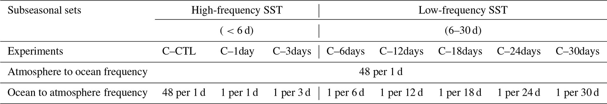
Table 1 Two sets of experiments with different SST feedback frequencies: high frequency (C–CTL, C–1day, and C–3days) and low frequency (C–6days, C–12days, C–18days, C–24days, and C–30days).

2.2 Experimental design

In this study, we investigated the role of oceanic FF using coupled CAM5–SIT and atmosphere-only CAM5 (A–CTL). Previous studies (Lan et al., 2022; Tseng et al., 2022) have provided a detailed description of the every time step coupling CAM5–SIT model and its performance in simulating the MJO. Table 1 displays the experimental configuration, incorporating monthly HadISST1 (uncoupled region) and ice concentrations over a 30-year period centered around the year 2000 (F2000 compsets; Rasch et al., 2019). Solar insolation, greenhouse gas and ozone concentrations, as well as aerosol emissions representative of present-day conditions were prescribed. In the A–CTL, observed monthly-mean SST around the year 2000 was prescribed to force the CAM5. For the coupled simulations, we adjusted the flux coupler (CPL) restriction in the Climate Earth System Model (CESM1; Hurrell et al., 2013) by implementing asymmetric exchange frequencies between the atmosphere and the ocean. The ocean continuously receives atmospheric forcing at every time step (30 min) and the temperature changes accordingly, but the SST seen by the atmospheric model is fixed at each time step for a specified time span (e.g., 1, 3, 6, 12, 18, 24, and 30 d); that is, the SST seen by the atmospheric model only changed until the end of the specified time span.

Two sets of experiments in addition to the A–CTL were conducted, each representing a different SST feedback frequency:

1. High-frequency SST feedback set. This set includes the control experiment (C–CTL) with SST feedback at every time step (FF as 48 per 1 d), once a day (C–1day: FF as 1 per 1 d), and every 3 d (C–3days: FF as 1 per 3 d).

2. Low-frequency SST feedback set. This set includes experiments with SST feedback to the atmosphere for every 6 d (C–6days: FF as 1 per 6 d), 12 d (C–12days: FF as 1 per 12 d), 18 d (C–18days: FF as 1 per 18 d), 24 d (C–24days: FF as 1 per 24 d), and 30 d (C–30days: FF as 1 per 30 d).

The SIT is coupled to CAM5 between 30° N and 30° S. The ocean was weakly nudged (using a 30 d exponential timescale) between depths of 10.5 and 107.8 m, and strongly nudged (using a 1 d exponential timescale) below 107.8 m, based on the climatological ocean temperature data from NCEP Global Ocean Data Assimilation System (GODAS). No nudging was applied in the uppermost 10.5 m, allowing the simulation of rigorous air–sea coupling near the ocean surface.

During the simulation, the SIT recalculated the SST within the tropical air–sea coupling region. Outside this coupling region, the annual cycle of HadSST1 was prescribed. No SST transition between the tropical air–sea coupling zone and the extratropical SST-prescribed regions was applied. The ocean bathymetry for the SIT was derived from the NOAA's 1 arcmin global relief model of earth's surface that integrated land topography and ocean bathymetry (ETOPO1) data (Amante and Eakins, 2009). To ensure consistency and comparability, all observational, atmospheric, oceanic, and reanalysis data were interpolated into a horizontal resolution of 1.9° × 2.5° for model initialization, nudging, and comparison of experimental simulations.

2.3 Methodology

The analysis focused on the boreal winter period (November to April), the season with the most pronounced eastward propagation of the MJO. To identify intraseasonal variability, the CLIVAR MJO Working Group diagnostics package (CLIVAR Madden–Julian Oscillation Working Group, 2009) and a 20–100 d filter (Wang et al., 2014) were used. MJO phases were defined based on the Real-time Multivariate MJO series 1 (RMM1) and series 2 (RMM2) proposed by Wheeler and Hendon (2004), which utilized the first two principal components of combined near-equatorial OLR and zonal winds at 850 and 200 hPa. The bandpass-filtered data were used to calculate the index and define the MJO phases.

Analysis of column-integrated MSE budgets was conducted to investigate the association between tropical convection and large-scale circulations. The column-integrated MSE budget equation (e.g., Sobel et al., 2014) is approximately given by

$$\begin{array}{}\text{(1)}& \begin{array}{rl}{〈{\displaystyle \frac{\partial h}{\partial t}}〉}^{\prime }& =-{〈u{\displaystyle \frac{\partial h}{\partial x}}〉}^{\prime }-{〈v{\displaystyle \frac{\partial h}{\partial y}}〉}^{\prime }-{〈\mathit{\omega }{\displaystyle \frac{\partial h}{\partial p}}〉}^{\prime }\\ & +\langle \text{LW}{\rangle }^{\prime }+\langle \text{SW}{\rangle }^{\prime }+\langle \text{SH}{\rangle }^{\prime }+\langle \text{LH}{\rangle }^{\prime },\end{array}\end{array}$$

where h denotes the moist static energy:

$$\begin{array}{}\text{(2)}& h=c_{p}T+gz+L_{\mathit{\upsilon }}q,\end{array}$$

where T is temperature (K); q is specific humidity (Kg Kg⁻¹); c_p is dry air heat capacity at constant pressure (1004 J K⁻¹ kg⁻¹); L_υ is latent heat of condensation (taken constant at 2.5×10⁶ J kg⁻¹); u and v are horizontal and meridional wind (m s⁻¹), respectively; ω is the vertical pressure velocity (Pa s⁻¹); LW and SW are the longwave and shortwave radiation flux (W m⁻²), respectively; and LH and SH are the latent and sensible surface heat flux (W m⁻²), respectively. The angle bracket (〈*〉) represents mass-weighted vertical integration from 1000 to 100 hPa, and the intraseasonal anomalies are represented as $\langle *{\rangle }^{\prime }$

3 Results

3.1 The mean state and intraseasonal variability in SST

The variability in SST plays a crucial role in the dynamics of the MJO. Studies based on observations from TOGA COARE and DYNAMO revealed that MJO events exhibited a stronger ocean temperature response compared with average conditions (de Szoeke et al., 2014). Wu et al. (2021) revealed that the better MJO prediction skill in the CGCM could be attributed to the improved representation of high-frequency SST fluctuations related to the MJO, with warm (cold) SST anomalies to the east (west) of MJO convection, through the convection–SST feedback processes (T. Li et al., 2020; Wu et al., 2021). It is therefore necessary to check on the influences of coupling and coupling frequency on the SST fluctuations.

Table 2 Key intraseasonal (20–100 d bandpass filtered) ocean temperatures in all experiments: SST, differences between SST, and temperatures at 10 m depth (${\stackrel{\mathrm{‾}}{\mathrm{\Delta }T}}_{\mathrm{0}-\mathrm{10}\mathrm{m}}$) and 30 m depth (${\stackrel{\mathrm{‾}}{\mathrm{\Delta }T}}_{\mathrm{0}-\mathrm{30}\mathrm{m}}$); t max/mini SST and 10 m-depth temperature (T_10 m) in the area of (5–15° S, 110–130° E) during an MJO cycle for the observation (OISST); AGCM (A–CTL); high-frequency experiments (C–CTL, C–1day, and C–3days); and low-frequency experiments (C–6days, C–12days, C–18days, C–24days, and C–30days).

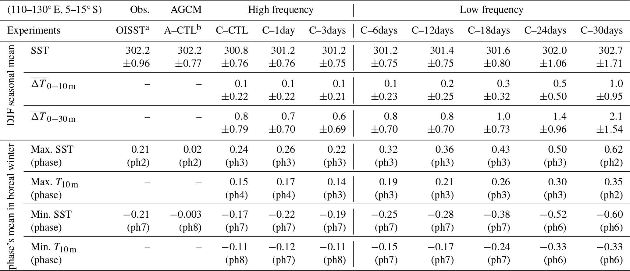
^a Daily average data, ^b monthly average data.

Table 2 presents the oceanic temperature anomalies for the December–January–February (DJF) seasonal mean, including the differences in oceanic temperature between the SST and depths of 10 m (${\stackrel{\mathrm{‾}}{\mathrm{\Delta }T}}_{\mathrm{0}-\mathrm{10}\mathrm{m}}$) and 30 m (${\stackrel{\mathrm{‾}}{\mathrm{\Delta }T}}_{\mathrm{0}-\mathrm{30}\mathrm{m}}$), as well as 20–100 d maximum and minimum SST and oceanic temperature at 10 m depth (T_10 m). The region of 5–15° S and 110–130° E was selected because of the largest variation in the 20–100 d bandpass-filtered SST when the MJO passes over the Indo-Pacific region. Simulated DJF seasonal mean SST (300.8–302.0 K) are generally smaller than OISST (302.2 K) but increase with the lower SST feedback frequency except in C–30days (302.7 K), while the SST standard deviation remains within 0.8 K, smaller than OISST (0.96 K), except in C–24days (1.06 K) and C–30days (1.71 K) which implies the potential jump in SST.

The simulated subsurface (0–10 and 0–30 m) ocean temperatures were compared with those in the NCEP GODAS reanalysis and presented as (${\stackrel{\mathrm{‾}}{\mathrm{\Delta }T}}_{\mathrm{0}-\mathrm{10}\mathrm{m}}$ and ${\stackrel{\mathrm{‾}}{\mathrm{\Delta }T}}_{\mathrm{0}-\mathrm{30}\mathrm{m}}$). The ${\stackrel{\mathrm{‾}}{\mathrm{\Delta }T}}_{\mathrm{0}-\mathrm{10}\mathrm{m}}$ in high-frequency experiments maintained a 0.1 K temperature difference. In low-frequency experiments, ${\stackrel{\mathrm{‾}}{\mathrm{\Delta }T}}_{\mathrm{0}-\mathrm{10}\mathrm{m}}$ increased from 0.2 to 1.0 K with decreasing SST feedback frequency. The temperature difference (${\stackrel{\mathrm{‾}}{\mathrm{\Delta }T}}_{\mathrm{0}-\mathrm{30}\mathrm{m}}$) in both high-frequency and low-frequency experiments remained approximately 0.8 K, except for C–24days and C–30days with an increase as high as 1.4 and 2.1 K, respectively, with larger standard deviations. The comparison revealed the cooling effect of the SIT on the seasonal mean SST, especially in the higher-frequency coupling experiment, due to the more rigorous heat exchanges between ocean and atmosphere. However, in the lower-frequency experiments, the SST became much warmer and so did vertical temperature differences due likely to the unrealistically large heat accumulation of loss in the ocean.

As for the MJO simulation, the SST fluctuation is more relevant. The OISST fluctuation through an MJO cycle was about ±0.21 K. In comparison, the uncoupled A–CTL, which was forced by monthly mean HadISST1, yielded a negligible SST fluctuation (−0.003–0.02 K) as expected. In the high-frequency experiments, SST fluctuated in magnitudes similar to that in the daily OISST. The amplitude became unrealistically larger in the low-frequency coupling experiments with C–30days reaching as high as 0.6 K. The increasingly larger amplitudes likely resulted from the heat accumulation in the ocean because of less frequent feedback (or heat release) to the model atmosphere. Changes in coupling frequency led to different amplitudes of SST fluctuation in an MJO cycle. As will be revealed later, this effect had marked influence on the MJO simulations.

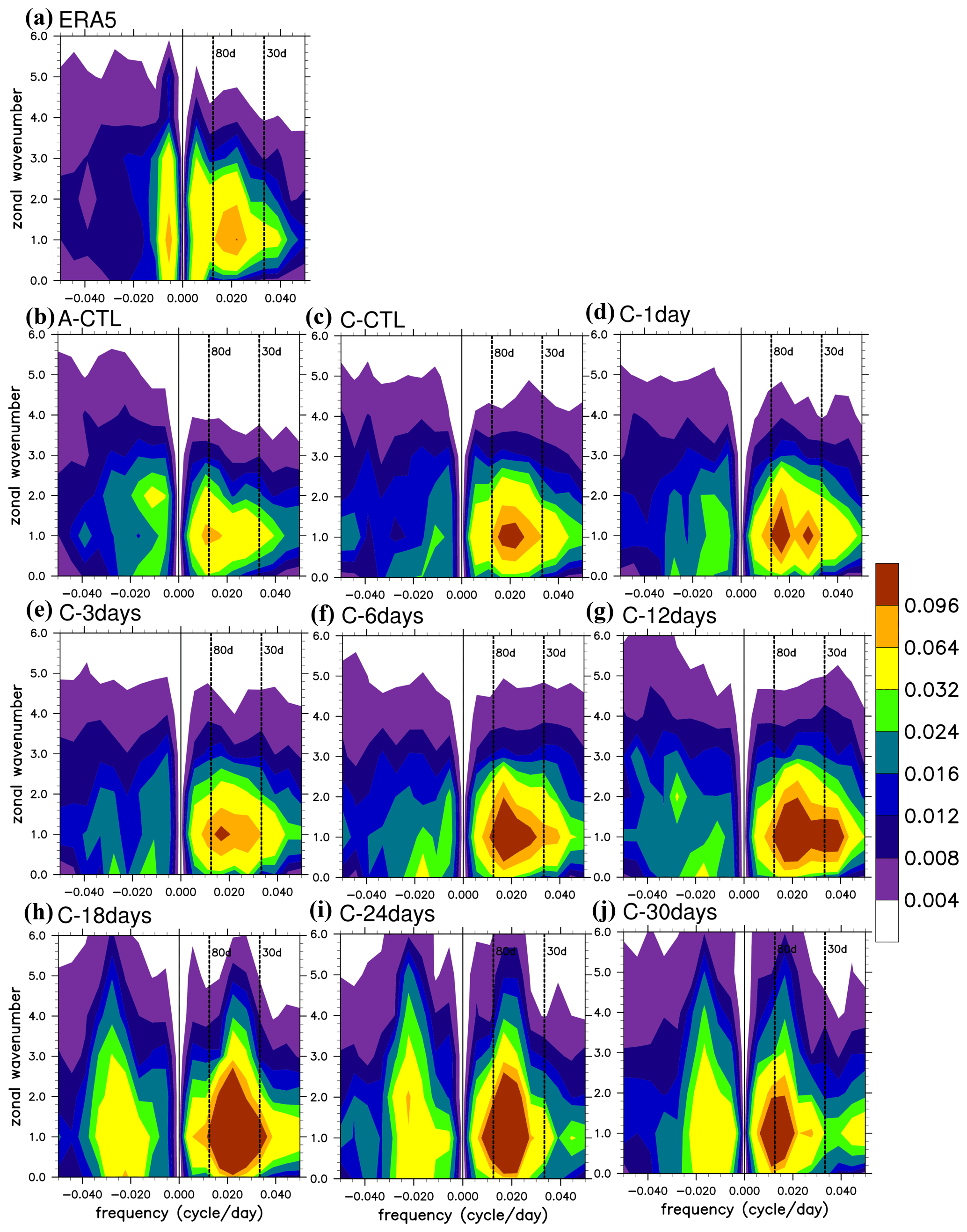
Figure 1 Wavenumber–frequency spectra for 850-hPa zonal wind averaged over 10° S to 10° N in boreal winter after removing the climatological mean seasonal cycle. Vertical dashed lines represent periods at 80 and 30 d. Panels (a)–(j) are from ERA5 reanalysis: A–CTL, C–CTL, C–1day, C–3days, C–6days, C–12days, C–18days, C–24days, and C–30days, respectively.

3.2 MJO simulation: high-frequency and low-frequency SST feedback experiments

3.2.1 General structure

The propagation characteristics of the different experiments were analyzed using the wavenumber–frequency spectrum (W–FS). The spectra of unfiltered U850 in ERA5, A–CTL, and all coupling experiments with different feedback frequency are shown in Fig. 1a–j. The C–CTL experiment accurately captures the eastward propagating signals at zone wavenumber 1 with a 30–80 d period (Fig. 1a and c), although with a slightly larger amplitude than ERA5 (Fig. 1a). By contrast, the uncoupled A–CTL produced an unrealistic spectral shift to timescales longer than 30–80 d (Fig. 1b) and simulated the unrealistic westward propagation at wavenumber 2.

The W–FS spectra of the C–1day and C–3day experiments showed two peaks for zone wavenumber 1 over the 30–80 d period. The low-frequency experiments (i.e., from C–6days to C–30days) increasingly enhanced the amplitudes and lowered the frequency of intraseasonal perturbations with decreasing feedback frequency. Furthermore, unrealistic westward W–FS of U850 becomes evident in Fig. 1h and i in the C–18days, C–24days, and C–30days experiments, reflecting the stationary nature of simulated MJO seen in Fig. 2i and j.

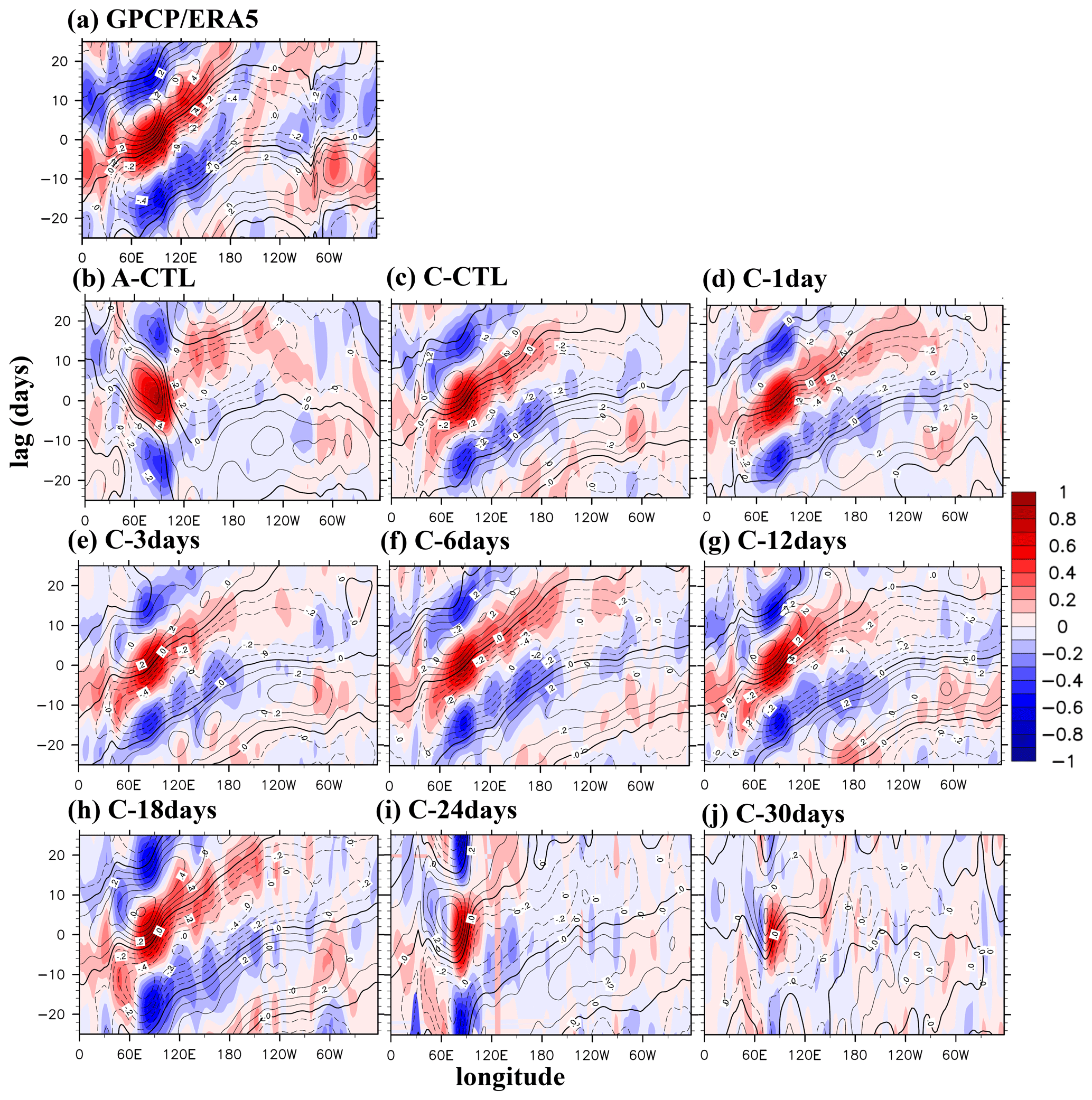
Figure 2 Hovmöller diagrams of correlation between precipitation averaged over 10° S to 5° N, 75–100° E, as well as precipitation (colors) and 850 hPa zonal wind (contours) averaged over 10° N to 10° S. Panels (a)–(j) are arranged in the same order as in Fig. 1 for GPCP/ERA5 and all experiments. All data are 20–100 d bandpass filtered.

The Hovmöller diagrams in Fig. 2a–j depict the evolution of 10° N to 10° S averaged precipitation and U850 anomalies on intraseasonal timescales, represented by the lagging correlation coefficients with the precipitation averaged over 10° S to 5° N, 75–100° E. In GPCP/ERA5, observed precipitation and U850 propagated eastward from the eastern IO to the dateline, with precipitation leading U850 by approximately a quarter of a cycle and a propagation speed of about 5 m s⁻¹ (Fig. 2a). The A–CTL simulation was dominated by stationary features, with westward-propagating tendency over the IO and weak and slow eastward propagation over the Maritime Continent (MC) and WP (Fig. 2b). The Hovmöller diagrams derived from high-frequency and low-frequency experiments (Fig. 2c, d, e, f, g, and h) display the key eastward propagation characteristics in both precipitation and U850, as well as the phase relationship between them, except in C–24days and C–30days which were dominated by stationary perturbations. Further decreased feedback frequency from 1 per 24 d to 1 per 30 d also further weakened the signals of precipitation and U850. More detailed discussion on this topic will be presented in the subsequent section.

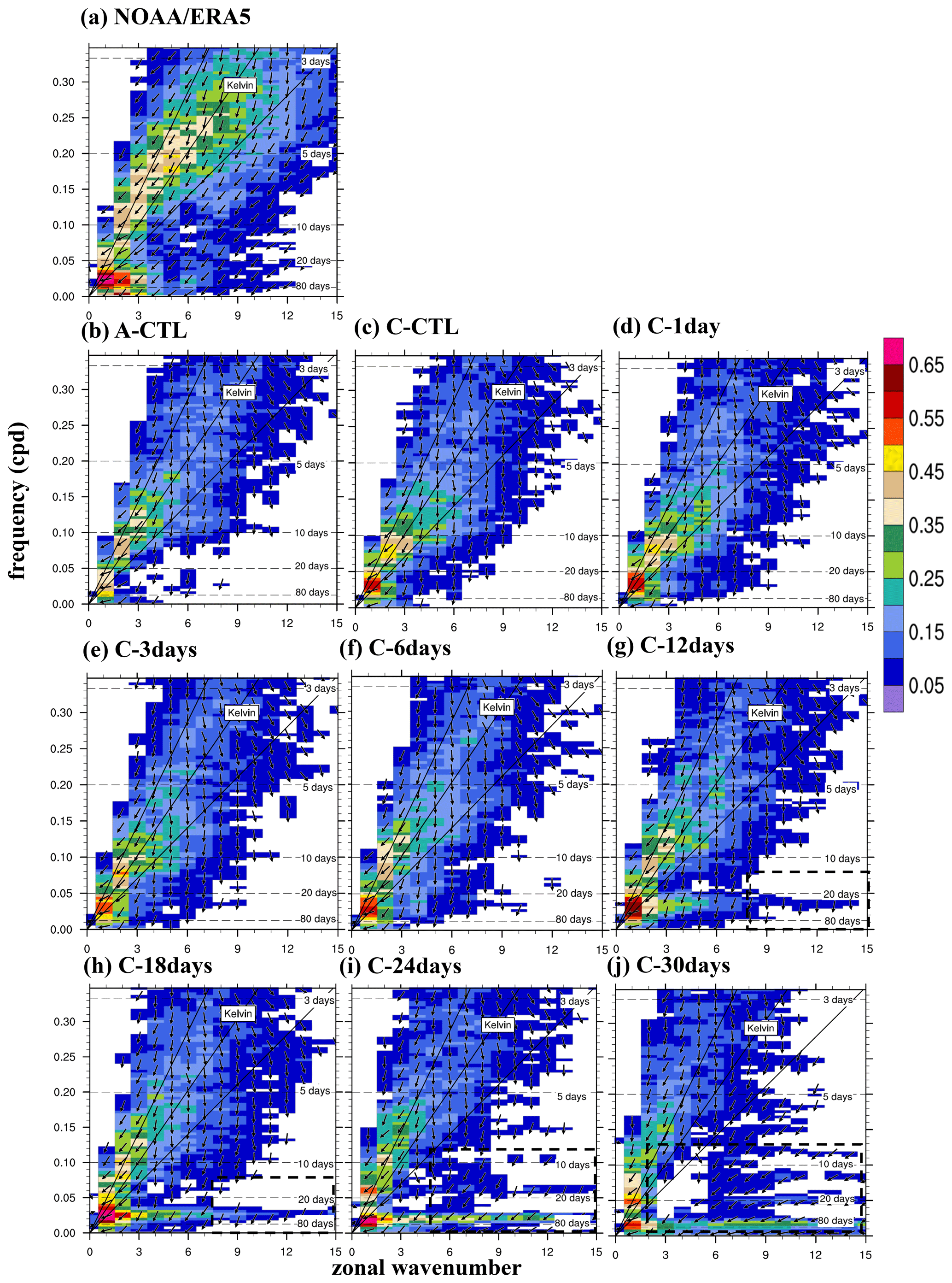
Figure 3 Zonal wavenumber–frequency power spectra of anomalous OLR (colors) and phase lag with U850 (vectors) for the symmetric component of tropical waves, with the vertically upward vector representing a phase lag of 0° and phase lag increasing clockwise. Three dispersion straight lines with increasing slopes representing the equatorial kelvin waves (derived from the shallow water equations) corresponding to three equivalent depths: 12, 25, and 50 m, respectively. Panels (a)–(j) are arranged in the same order as in Fig. 1 for NOAA/ERA5 and all experiments.

We conducted a wavenumber–frequency power spectral analysis (Wheeler and Kiladis, 1999) to examine the phase lag and coherence between the tropical circulation and convection. Figure 3a–i illustrate the symmetric part of OLR and U850 for NOAA/ERA5 data and all model experiments. The MJO band exhibits a high degree of coherence, indicating a strong correlation between the NOAA MJO-related OLR signal and wavenumbers 1–3 (Fig. 3a). The phase lag in the 30–80 d band is approximately 90°, consistent with previous studies (Ren et al., 2019; Wheeler and Kiladis, 1999). All model experiments simulated the coherence within wavenumber 3 in the MJO band, with a phase lag similar to that of NOAA/ERA5 data. However, the A–CTL spectrum exhibits only half of the observed coherence peak at wavenumber 1, and also weaker coherence at wavenumbers 2–3 for the 30–80 d period compared with NOAA/ERA5 data. The experiments C–CTL, C–1day, C–3days, C–6days, C–12days, and C–18days yielded a wavenumber-1 coherence peak similar to that in NOAA/ERA5. Additionally, as the SST feedback frequency decreased from 1 per 12 to 1 per 30 d, the experiments increasingly simulated unrealistic coherence in the very low frequency with a wide range of zonal wavenumbers from 1 to 12 (Fig. 3g, h, i, and j), i.e., no zonal scale preference.

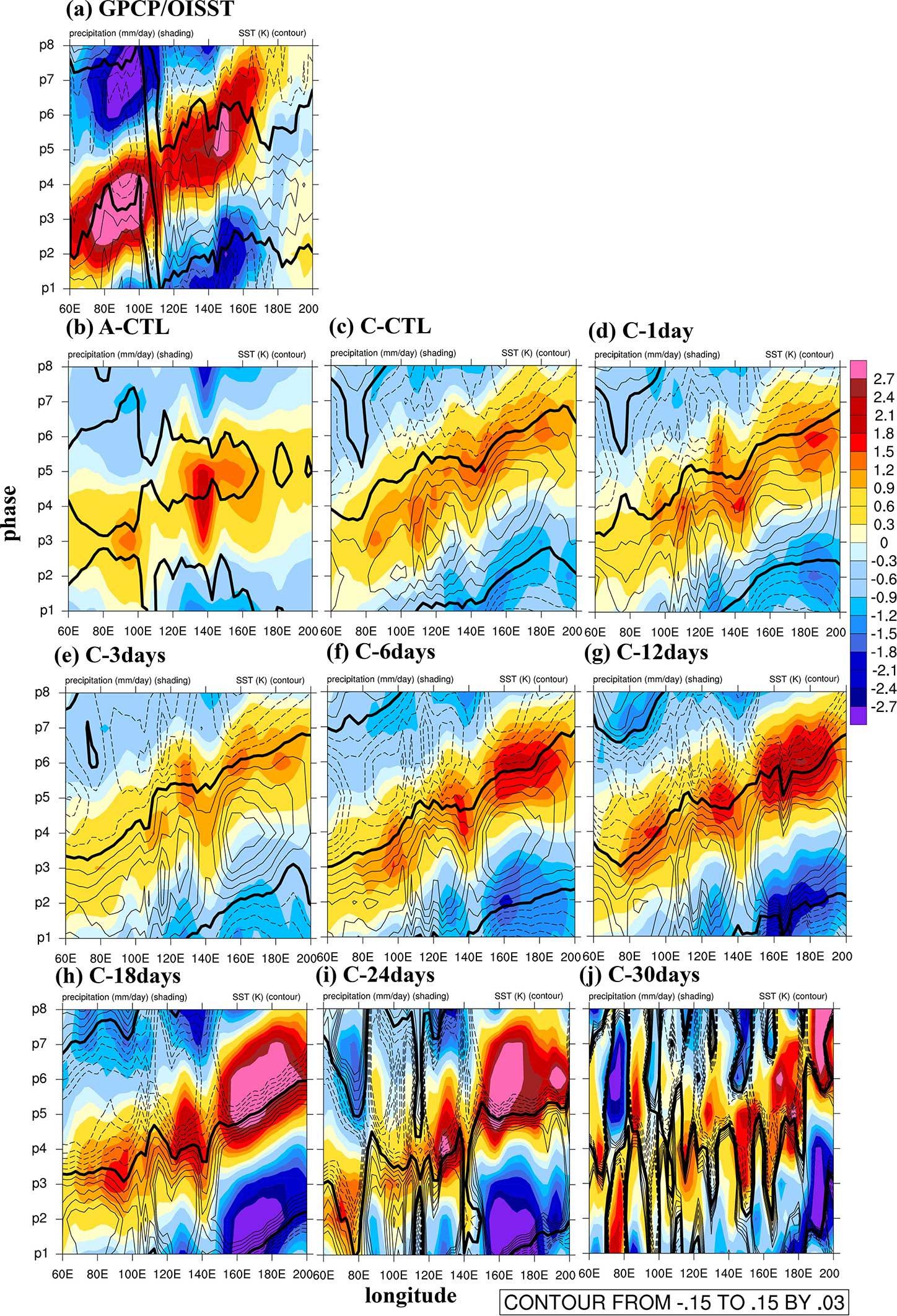
Figure 4 Phase–longitude Hovmöller diagrams of 20–100 d filtered precipitation (shading; in mm d⁻¹) and SST anomaly (contours; in degrees K) averaged over 10° N to 10° S from phases 1–8. Contour interval is 0.03. Solid, dashed, and thick-black curves represent positive, negative, and zero values, respectively. Panels (a)–(j) are arranged in the same order as in Fig. 1 for NOAA/ERA5 and all experiments.

Figure 4 shows the phase–longitude diagrams in which the 20–100 d filtered precipitation (shaded) and SST (contour) anomalies were averaged over 10° S to 10° N to determine the relationship between precipitation and SST fluctuations and to provide insights into the connection between air–sea coupling and convection. As expected, the A–CTL did not simulate the eastward-propagating coupled SST–convection perturbations as in observation (Fig. 4a), whereas C–CTL, C–1day, and C–3days properly reproduced the observed features. The eastward-propagating coupled perturbations were also simulated in C–6days, C–12days, and C–18days, but with unrealistically increasing amplitudes near the dateline, especially in the C–18days experiment. The perturbation amplification near the dateline was likely due to the lack of ocean circulation in the CAM5–SIT. The amplification was also seen in C–24days which failed to simulate the eastward-propagating intraseasonal perturbations. When coupling frequency was reduced to 1 per 30 d, the eastward propagation could no longer be simulated and was replaced by unorganized standing oscillations in much smaller zonal scales.

Liang et al. (2018) suggested that SST leading precipitation by 10 d implies air–sea interactions at the intraseasonal timescale during MJO events, with SST playing a crucial role in modulating the MJO's intensity and propagation. The A–CTL simulation exhibited weak SST anomalies and stationary precipitation when using the monthly average HadISST1. By contrast, the C–24days and C–30days experiments showed no clear phase lag between unorganized SST and precipitation perturbations. A comparison between simulation results and observation indicates that the air–sea interaction plays a crucial role in facilitating eastward propagation and higher frequency feedback yields more realistic simulations.

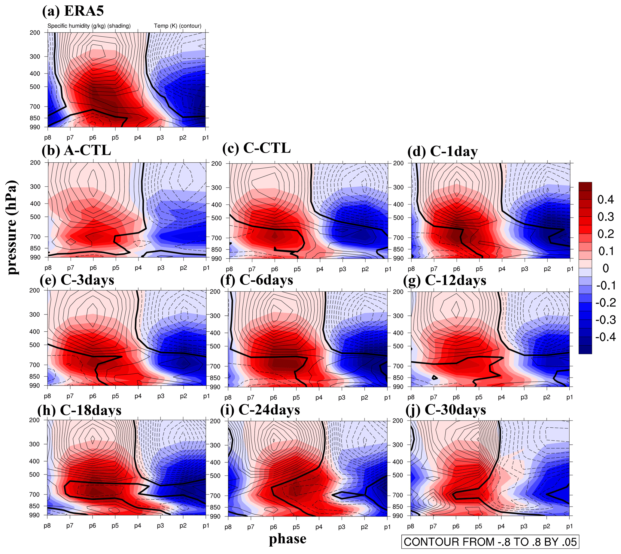
Figure 5 Phase–vertical Hovmöller diagrams of 20–100 d specific humidity (shading; in g kg⁻¹) and air temperature (contours; in degrees K) averaged over 5–20° S to 120–150° E. Solid, dashed, and thick-black curves are positive, negative, and zero values, respectively. Panels (a)–(j) are arranged in the same order as in Fig. 1 for NOAA/ERA5 and all experiments.

3.2.2 Vertical structures of the MJO in the atmosphere

Air–sea interaction plays a significant role in influencing atmospheric moisture and convection associated with the MJO (Savarin and Chen, 2022). Whereas the ocean to the east of deep convection warmed due to more downwelling shortwave radiation and less heat fluxes into the atmosphere associated with weaker winds, near-surface moisture convergence under the anomalous subsidence over the warmer water preconditioned the eastward movement of the deep convection (DeMott et al., 2015; Zhang, 2005). The MJO was noted to detour southward when crossing the MC region, exhibiting enhanced convective activity preferentially in the southern MC area and weaker convection in the central MC area (Hsu and Lee, 2005; Wu and Hsu, 2009; Kim et al., 2017). Hovmöller diagrams in Fig. 5a–j illustrate the relationship between the vertical structure of air temperature (contours; in degrees K) and specific humidity (shading; in g kg⁻¹) anomalies from the surface to 200 hPa averaged over 5–20° S and 120–150° E. In ERA5, the lower-level positive temperature anomaly in phase 3 (i.e., preconditioning phase) leads to the development of deep temperature and moisture anomalies (i.e., deep convection) after phase 4 over the MC, when moisture anomalies reached the maxima at 700–500 hPa. This two-phase upward development was not properly simulated in A–CTL, which shows a sudden switch between positive and negative anomalies in the entire troposphere, instead of progressively upward development with time. The upward development was generally simulated in coupled simulations from C–CTL to C–6days (Fig. 5c, d, and e), although the negative temperature anomalies below 500 hPa were over-simulated after phase 5. It became less well simulated beyond C–12days and was gradually replaced by a sudden phase switch as in the A–CTL, especially in C–30days (Fig. 5f, g, h, i, and j). The preconditioning phase completely disappears in C–18days and beyond. As identified in previous studies, the two-phase upward development is a manifestation of air–sea coupling. The missing of this coupling evidently resulted in the poor simulation in the A–CTL and extremely low feedback frequency experiments.

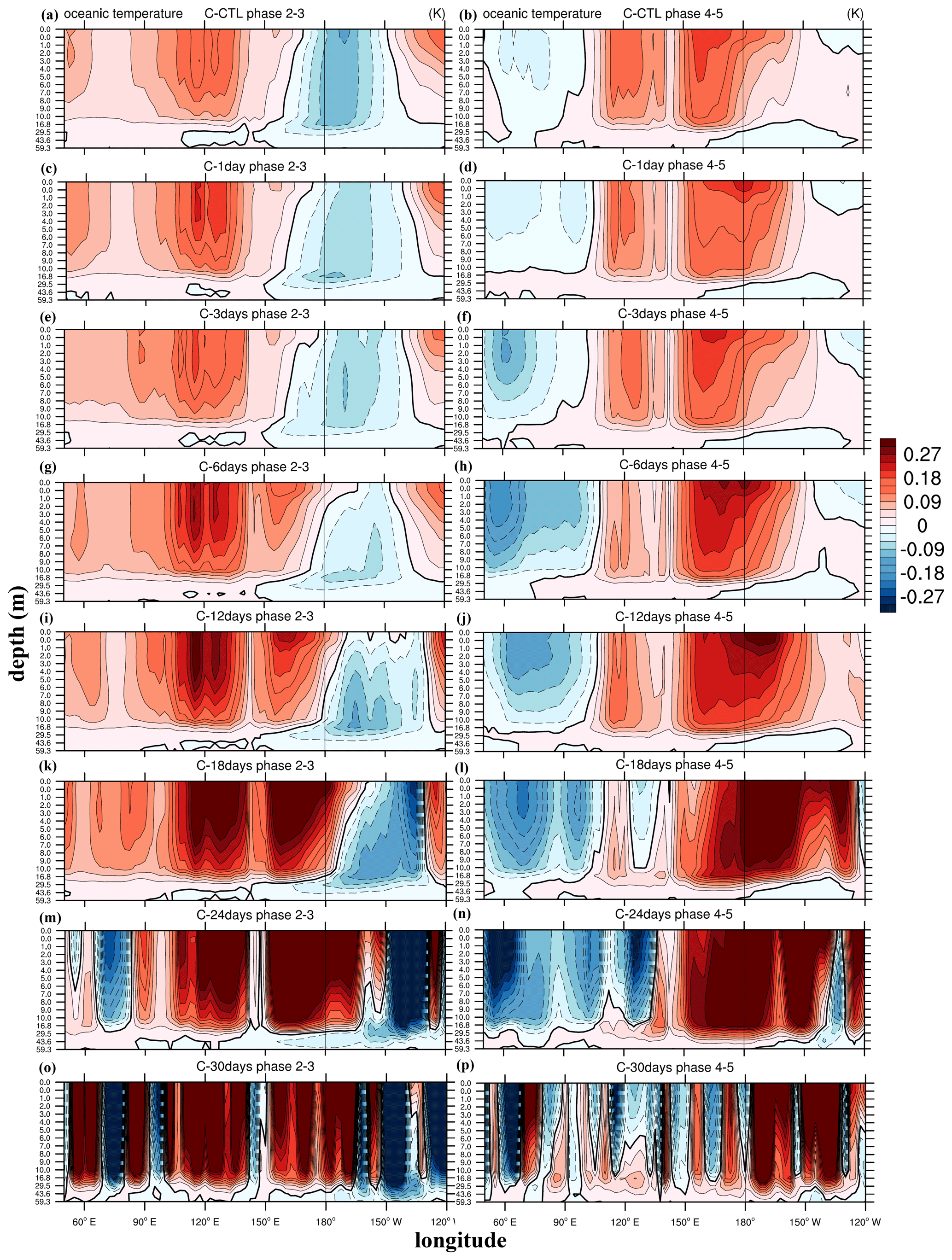
Figure 6 The 20–100 d filtered oceanic temperature (shading and contours; interval 0.03; in degrees K) at phases 2 and 3 (left column) and phases 4 and 5 (right column) averaged over 0–15° S between 0 and 60 m depth. Panels (a) and (b) are from C–CTL, (c) and (d) are from C–1day, (e) and (f) are from C–3days, (g) and (h) are from C–6days, (i) and (j) are from C–12days, (k) and (l) are from C–18days, (m) and (n) are from C–24days, and (o) and (p) are from C–30days.

3.2.3 Vertical structures of the MJO in the ocean

The 1-D turbulence kinetic energy (TKE) ocean model incorporates a high vertical resolution that captures the vertical gradient of temperature in the upper ocean. Figure 6 (left column) illustrates the vertical structures of oceanic temperature between 0 and 60 m during phases 2 and 3 when the deep convection occurred over the eastern IO (60–90° E) and easterly anomalies prevailed over the MC and western Pacific. In the high-frequency experiments (Fig. 6a, c, and e), the upper oceanic temperatures exhibit warming patterns within 30 m depth at 100–140° E (i.e., east of the deep convection and under the easterly anomalies), apparently due to more downwelling shortwave radiation and less heat flux release into the atmosphere. By contrast, the cooling near the dateline was associated with westerly anomalies. With decreasing feedback frequency, the cooling to the east of 150° E seen in high-frequency experiments was replaced by oceanic warming that was amplified with further feedback frequency decrease. The warming region that became more widespread and the larger amplitude with less frequent feedback eventually grew to cover the entire IO and WP, an area much larger than the scale of the atmospheric MJO. The mismatch between the atmospheric and oceanic anomalies suggested the weakening atmosphere–ocean coupling that resulted in poor simulation of the MJO in the low-frequency-feedback simulations. The emergence of small-scale unorganized structures with decreasing feedback frequency is also evident in phases 4 and 5 (right column in Fig. 6), e.g., negative ocean temperature anomalies in the Indian Ocean under the prevailing westerly anomalies.

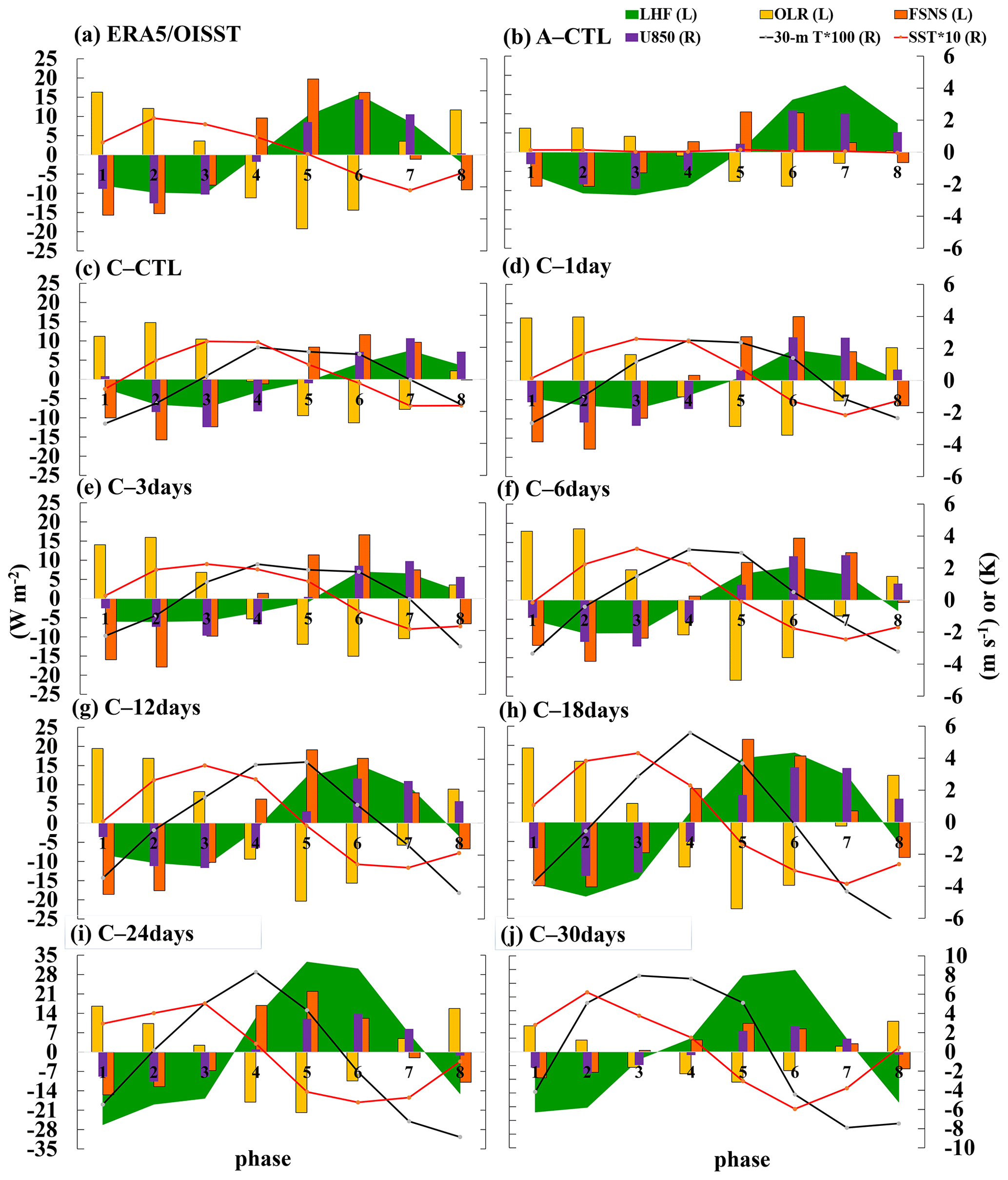
Figure 7 The lead–lag relationship between MJO-related atmosphere and SST variation from phases 1–8 averaged within 5–15° S and 110–130° E. The variables analyzed include 20–100 d filtered LHF (green shading), OLR (yellow bars), FSNS (orange bars), U850 (purple bars), 30 m T (multiplied by 100; black line), and SST (multiplied by 10; orange line). Variables denoted with L (R) are scaled by the left (right) y axis. Panels (a)–(j) are from ERA5/OISST reanalysis: A–CTL, C–CTL, C–1day, C–3days, C–6days, C–12days, C–18days, C–24days, and C–30days, respectively.

4 Discussion

4.1 Dynamic lead–lag relationship in intraseasonal variability

The lead–lag relationship refers to a situation where one variable (leading) is cross-correlated with the values of another variable (lagging) in subsequent phases, particularly in the case of SST fluctuations and MJO-related atmospheric variations between phases 1 and 8 within the domain of 5–15° S and 110–130° E (Fig. 7). The analyzed variables include 20–100 d filtered latent heat flux (LHF; indicated by green shading), OLR (indicated by yellow bars), net solar flux at surface (FSNS; represented by orange bars), U850 (indicated by purple bars), 30 m depth oceanic temperature (30 m T multiplied by 100; indicated by a black line), and SST (multiplied by 10; indicated by an orange line). A positive value in LHF and FSNS represents an upward flux from ocean to atmosphere.

A decrease in LHF, which indicates a reduction in heat loss from the ocean, and a negative FSNS, indicating that solar radiation is heating the ocean, coincide with an easterly anomaly that contributes to a positive SST anomaly in ERA5 (Fig. 7a). Reversed fluxes are associated with westerly anomalies. This lead–lag relationship depicts the in situ atmospheric forcing on the oceanic variability during an MJO. As the MJO convection progresses through the region (5–15° S, 110–130° E), several changes in atmospheric and oceanic variables occur. These changes include a shift in OLR from positive to negative values, a decrease in SST, a transition to westerly winds, and an increase in positive FSNS and LHF (Fig. 7a). The temporal variations in SST anomaly from C–CTL to C–12days were predominantly influenced by FSNS, with LHF playing a secondary role, similar to the findings of Gao et al. (2020a). With the exception of experiments of A–CTL, C–24days, and C–30days, both the high-frequency and low-frequency SST feedback experiments simulated similar lead–lag relationships to those in ERA5 (Fig. 7c, d, e, f, g, and h). In the C–24days and C–30days experiments, LHF was the largest flux term (note the different vertical scale for the two experiments), whereas the wind, OLR, and FSNS anomalies were much weaker than in other experiments. In the A–CTL experiment, which was forced by monthly HasISST1 data, the SST anomalies were small as expected, whereas fluxes, although weak, were still evident in response to atmospheric perturbations (Fig. 7b). Conversely, in both C–24days and C–30days experiments, a misalignment in the lead–lag relationship was observed, accompanied by weak anomalies in OLR and FSNS (Fig. 7i and j). This disparity between LHF and wind was likely due to the unrealistically widespread and large oceanic warming as shown in Fig. 6m and o.

In the simulations, the maximum positive anomaly in 30 m T was delayed by one phase compared with SST, indicating the transfer of heat from the ocean surface into the upper ocean progressively. Similarly, the occurrence of the most negative 30 m T anomaly was also delayed by one phase compared with SST, revealing the buffering role of the upper ocean when the atmospheric component of the MJO extracted (or deposited) heat (energy) from (in) the ocean (Fig. 7c, d, e, f, g, h, and i). This delayed effect was also evident in the field campaign. Moreover, de Szoeke et al. (2015) observed that the warmest 10 m ocean temperature occurred a few days later than the peak temperature at 0.1 m. Additionally, the 0.1 m ocean temperature was typically as warm as, or warmer than, the 10 m temperature as seen in Fig. 6. In the extremely low-frequency feedback experiments, the amplitude of 30 m temperature became unrealistically large due likely to the continuous accumulation or loss of the ocean heat.

4.2 Unorganized perturbations in extreme frequency feedback scenarios

DeMott et al. (2014) noted that in uncoupled experiments, the NCAR CAM superparameterized version 3 (SPCAM3) exhibited strong eastward propagation when a 5 d running mean SST was prescribed, but relatively weaker propagation for monthly mean SST. This raises the question of how much SST feedback periodicity is necessary to maintain robust eastward propagation in coupled experiments. This tendency was also seen in our study, that is, slower propagation (or weaker tendency) with decreased feedback frequency until the C–24days experiment (Figs. 1–7). By 1 per 30 d, the perturbations became stationary.

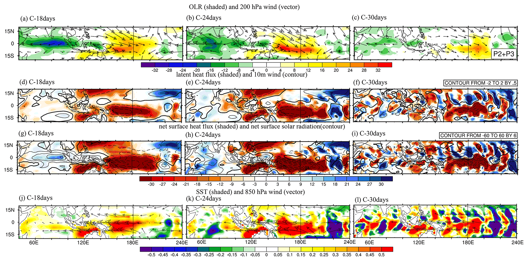
Figure 8 Averaged 20–100 d filtered fields at phases 2 and 3. (a–c) OLR (shaded; in W m⁻²), 200 hPa zonal and meridional wind anomaly (vector with reference vector shown at the top right corner; in m s⁻¹), latent heat flux (shaded; positive representing upward; in W m⁻²), and 10 m wind anomaly (contour interval 0.5; in m s⁻¹). (d–f) Net surface heat flux (shaded; in W m⁻²) and net solar radiation (contour interval 6; in W m⁻²). (g–i) SST (shaded; in degrees K) and 850 hPa zonal and meridional wind anomaly (vector with reference vector shown at the top right corner; in m s⁻¹). The number of days used to generate the composite is shown at the bottom right corner. Panels (a), (d), (g), and (j) are from C–18days, (b), (e), (h), and (k) are from C–24days, and (c), (f), (i), and (l) are from C–30days, respectively. Solid, dashed, and thick-black curves represent positive, negative, and zero values, respectively.

Generally, C–18days exhibited the unrealistic overestimation of intraseasonal variability while maintaining eastward propagation of the MJO. Here, we are not suggesting that C–18days represents the optimal SST feedback experiment. Figure 8 highlights the considerable differences in the simulation of MJO perturbations at phases 2 and 3 between C–18days and C–30days experiments. In C–18days, negative OLR anomalies were widespread from the western IO to the MC, while in reality it should be observed mainly in the IO and be accompanied by positive anomalies in the eastern MC, i.e., a west–east dipolar structure (Fig. 8a). In C–30days, the OLR anomaly, although still the dominant feature in the Indian Ocean–western Pacific region, became much weaker and characterized by smaller-scale perturbations. These OLR anomalies were generally associated with upper-level convergence (not shown) embedded in much weaker wind anomalies (U200) compared with those in C–18days. The circulation and OLR in C–24days exhibited characteristics similar to those in C–18days but with the OLR anomalies breaking up into smaller scales.

Furthermore, in the C–18days and C–24days experiments, negative anomalies indicative of a downward direction in LHF and net surface heat flux (Fig. 8d, e, g, and h) were predominantly observed in the convection-inactive region to the east of 150° E where low-level easterly wind and positive SST anomalies prevailed (Fig. 8j and k). The OLR, winds, heat fluxes, and SST to the west of 150° E exhibited similar correspondences between variables but in the opposite phase. With feedback frequency reduced to 1 per 30 d (Fig. 8f, i, and l), the heat fluxes and SST anomalies broke into unorganized smaller-scale features, consistent with the ocean temperature jump shown in Fig. 6h. Although the wind fields in both the upper and lower levels were still characterized by a large-scale structure, the corresponding divergences were dominated by much-smaller-scale perturbations (not shown), similar to heat fluxes and SST. The increasingly dominant smaller-scale perturbations can also be inferred from Figs. 2h–j and 4h–j. In addition, the large power spectra in the low-frequency band were spread across a wide range of wavenumbers, reflecting the smaller-scale nature of the simulated perturbations in C–30days (Fig. 3j). This imparity between the scale of rotational and divergent winds suggests the poor coupling between the convection and large-scale circulation.

With decreased feedback frequency of SST from C–CTL to C–30days, the ocean continued to receive atmospheric forcing, but the feedback response was delayed, leading to the accumulation or loss of energy (temperature) in the upper ocean, as seen in the SST distribution in the WP (Figs. 6 and 8). Subsequently, the C–30days experiment exhibited a comprehensive disorder over the Indo-Pacific region, with the SST anomalies showing an unrealistically erratic spatial distribution characterized by sudden jumps (Fig. 8l) associated with plus–minus latent heat flux and 10 m wind anomalies (Fig. 8f), net surface heat flux, and solar radiation (Fig. 8i). As a result, the organized large-scale circulation seen in the MJO did not manifest. To this extent, the air–sea interaction observed in the MJO no longer worked properly in the model.

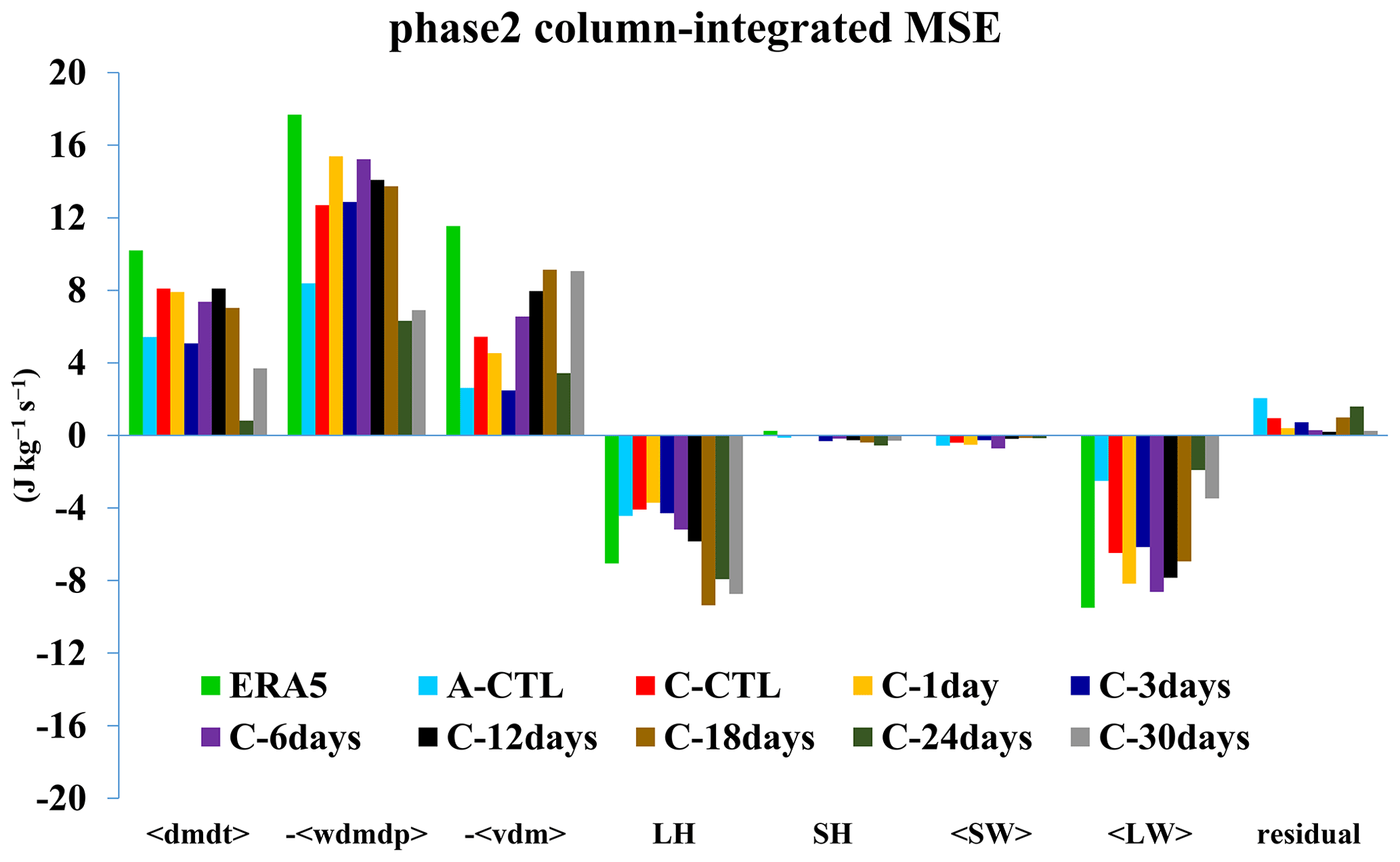
Figure 9 Averaged 20–100 d filtered column-integrated MSE budget terms (in J kg⁻¹ s⁻¹) in 0–10° S and 120–150° E for ERA5 and all model simulations. Colors represent different datasets: green for ERA5; light blue for A–CTL; red, orange, and dark blue for high-frequency experiments (C–CTL, C–1day, and C–3days, respectively); and purple, black, dark brown, dark green, and dark gray for low-frequency experiments (C–6days, C–12days, C–18days, C–24days, and C–30days, respectively). The bars from left to right represent MSE tendency (〈dmdt〉), vertical MSE advection (−〈wdmdp〉), horizontal MSE advection (−〈vdm〉), surface latent heat flux (LH), surface sensible heat flux (SH), shortwave radiation flux (〈SW〉), longwave radiation flux (〈LW〉), and residual terms.

4.3 Moist static energy budget analysis

We diagnosed the relative contribution of each term in Eq. (1) to the moist static energy (MSE) tendency with a focus on the second (preconditioning) and fifth (convection crossing the MC) phases. Figure 9 illustrates the physical processes associated with each term (averaged over 0–10° S and 120–150° E) contributing to the column-integrated MSE tendency (〈dmdt〉) in Eq. (1) during phase 2 in ERA5 and model simulations. In ERA5, when the MJO convection was in the eastern Indian Ocean, the column-integrated vertical and horizontal advection (−〈wdmdp〉 and −〈vdm〉) over the MC area were the dominant terms in the MSE budget and largely compensated by longwave radiation and latent heat flux, as reported in Wang and Li (2020) and Tseng et al. (2022). All experiments simulated the positive and negative contributions similar to those derived from ERA5 although with different amplitudes. Notably, the C–24days and C–30days simulated relatively weak vertical advection, too strong negative latent heat flux, and too weak longwave radiation flux. As a result, the C–24days and C–30days simulated a relatively weak tendency compared with other experiments. The results are consistent with the poor simulation of the MJO in the extremely low-frequency feedback experiments discussed above.

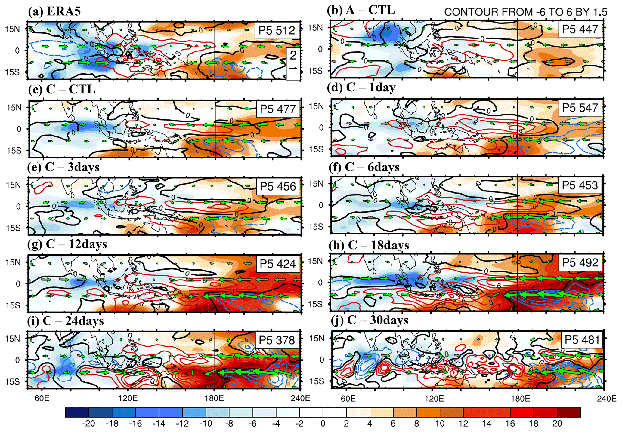
Figure 10 Filtered column-integrated MSE tendency (shading; in J kg⁻¹ s⁻¹), precipitation (contour interval 1.5; in mm d⁻¹), and 850 hPa wind (green vector with reference vector 2 m s⁻¹) in phase 5: (a) ERA5, (b) A–CTL, (c) C–CTL, (d) C–1day, (e) C–3days, (f) C–6days, (g) C–12days, (h) C–18days, (i) C–24days, and (i) C–30days. Solid-red, dashed-blue, and thick-black curves represent positive, negative, and zero values, respectively.

In Fig. 10, we compare the spatial distribution of column-integrated MSE tendency 〈dmdt〉 (shading), precipitation (contours), and 850 hPa wind (vectors) during phase 5, i.e., the period when the strongest convection crosses the MC. In ERA5, the main convection (indicated by a positive precipitation anomaly) is accompanied by low-level convergence in the 850 hPa wind across the MC extending into the WP (Fig. 10a). A positive 〈dmdt〉 is observed to the east of the MJO convection to the south of the Equator (Fig. 10a). Conversely, a negative tendency is observed to the west of the MJO convection accompanied by negative precipitation anomalies further to the west. The phase relationship between the MSE tendency and precipitation reflects the eastward-propagating nature of the MJO. With the exception of A–CTL, C–24days, and C–30days, the model simulations displayed a similar structure in the 20–100 d filtered 〈dmdt〉, precipitation, and 850 hPa wind vectors (Fig. 10c, d, e, f, g, and h), although the exact locations may be shifted compared with those derived from ERA5. The C–CTL simulated relatively weak signals compared with those of ERA5, whereas the signals became increasingly stronger with decreasing feedback frequency. The signals became unrealistically strong beyond 1 per 18 d feedback frequency and the lead–lag relationship between the MSE tendency and precipitation became less clear. For example, a positive precipitation anomaly became in phase with the tendency in the western Pacific south of the Equator in C–24days and C–30days experiments, and the tendency was much weaker in C–30days. The results were consistent with the weaker eastward propagation tendency in the low-frequency feedback experiments, especially in C–24days and C–30days when the feedback frequency became unrealistically low.

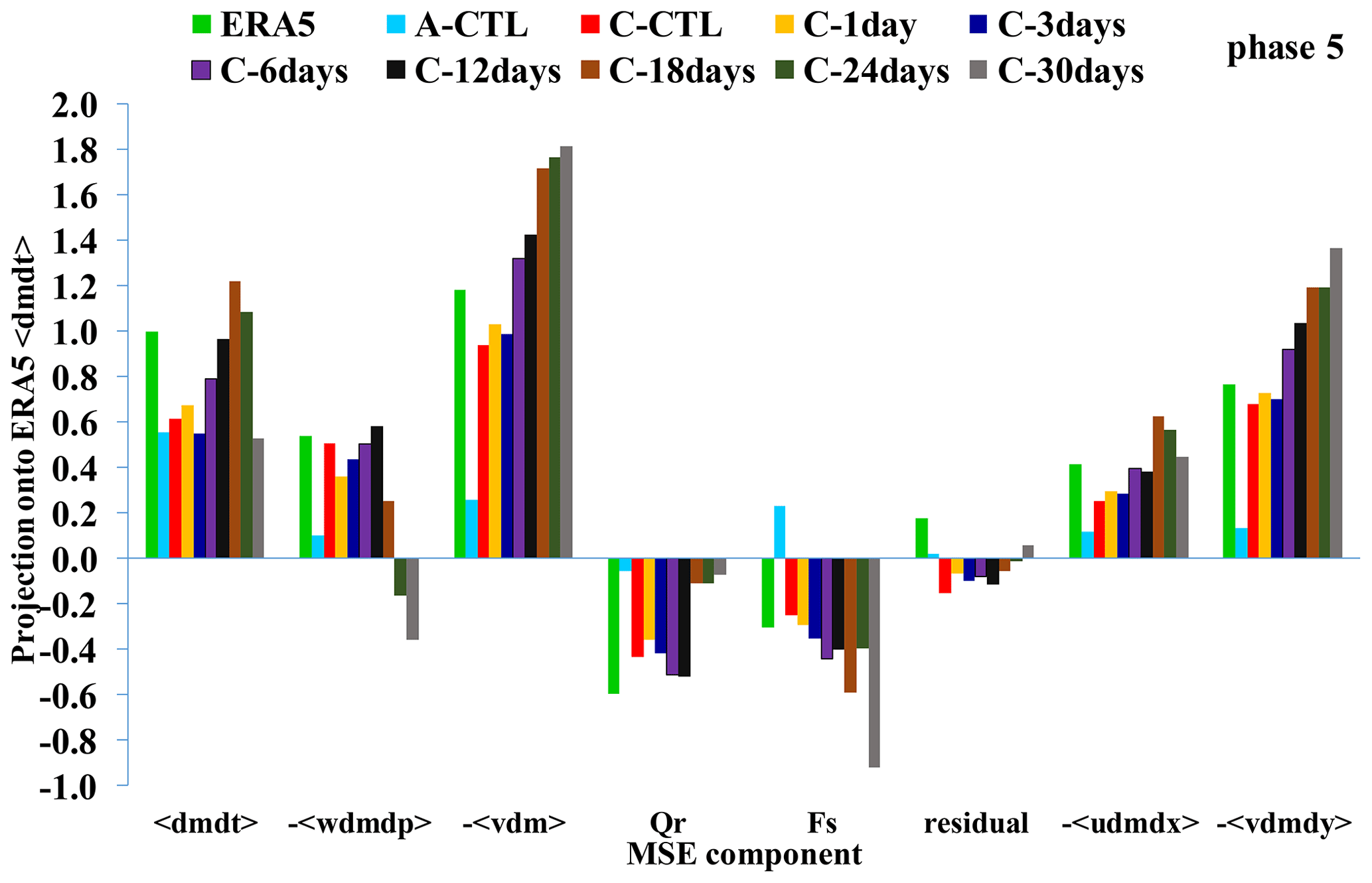
Figure 11 The projection of each MSE component onto the ERA5 column-integrated MSE tendency at phase 5 over the MC (20° S to 20° N, 90–210° E): 〈dmdt〉, −〈wdmdp〉, −〈vdm〉, Q_r, F_s, and residual; decomposition of horizontal MSE advection to zonal and meridional advection (−〈udmdt〉 and −〈vdmdy〉).

The corresponding MSE budget during phase 5 is shown in Fig. 10. The MC has been identified as a barrier to the eastward propagation of the MJO (Hsu and Lee, 2005; Wu and Hsu, 2009; Tseng et al., 2017; K. Li et al., 2020) and approximately 30 %–50 % of the MJO experienced stalling over the MC (Zhang and Han, 2020). To determine whether the MJO has sufficient energy to traverse the MC, we focused the analysis on phase 5. Figure 11 illustrates the projection of each MSE component and decomposition of the horizontal MSE advection at phase 5 over the MC region (20° S to 20° N, 90–210° E) following the approach of Tseng et al. (2022) and Jiang et al. (2018), where F_s is total surface fluxes including SH and LH, and Q_r is vertically integrated net SW and LW radiation. Unlike in phase 2 when vertical advection is the dominant term, the MSE tendency was dominated by the horizonal MSE advection −〈vdm〉 in ERA5 and all experiments, except the A–CTL. This contribution increased with decreasing SST feedback frequency. The weaker positive vertical advection −〈wdmdp〉 did not vary systematically with decreasing feedback frequency and even turned negative in C–24days and C–30days. Fs and Q_r acted to damp the tendency by canceling out the effect of the advection term. F_s tended to be more negative with decreasing feedback frequency and became much larger in C–30days. By contrast, Q_r was unrealistically weak in C–18days, C–24days, and C–30days. The uncoupled simulation yielded much weaker amplitude in all terms as expected.

The −〈vdm〉 that contributed most to the eastward propagation of the MJO in phase 5 was further decomposed into zonal (−〈udmdx〉) and meridional (−〈vdmdy〉) components to examine their relative effects (Fig. 11). Both components contributed positively, but the −〈vdmdy〉 exhibited a larger amplitude, consistent with Tseng et al. (2015, 2022). The −〈vdmdy〉 of high-frequency SST feedback experiments yielded results closely similar to those of ERA5. Comparatively, the −〈vdmdy〉 term in low-frequency SST feedback experiments (C–18days, C–24days, and C–30days) became unrealistically large with decreasing feedback frequency and the potential jump in SST.

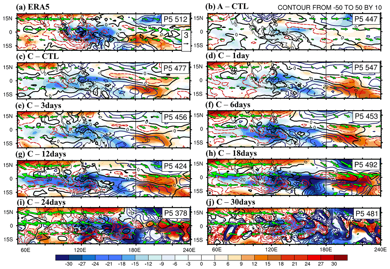
Figure 12 Filtered column-integrated vertical (shading; in J kg⁻¹ s⁻¹) and horizontal MSE advection (contour interval 6.0; in J kg⁻¹ s⁻¹), as well as 200 hPa wind (green vector with reference vector 3 m s⁻¹): (a) ERA5, (b) A–CTL, (c) C–CTL, (d) C–1day, (e) C–3days, (f) C–6days, (g) C–12days, (h) C–18days, (i) C–24days, and (j) C–30days. Solid-blue, dashed-red, and thick-black curves represent positive, negative, and zero values, respectively.

Spatial distributions of −〈wdmdp〉, −〈vdm〉, and 200 hPa wind at phase 5 are shown in Fig. 12. In ERA5, the wind divergence at 200 hPa at phase 5 (Fig. 12a) overlaid the 850 hPa convergence (Fig. 10a), reflecting a deep convection structure. The model simulations exhibited a similar structure to ERA5 except in A–CTL, C–24days, and C–30days experiments, and again the amplitude increased with decreasing feedback frequency. In ERA5, negative −〈wdmdp〉 and −〈vdm〉 anomalies (Fig. 12a) were observed to the west of the MJO convection (Fig. 10a). The spatial distribution of the negative −〈vdm〉 anomaly (dashed-red contours) extends from the IO to the MC and the positive anomaly (predominantly meridional advection from the south; not shown) in the western–central Pacific south of the Equator tends to facilitate the eastward propagation of deep convection in the western Pacific, consistent with Tseng et al. (2015, 2022). The −〈wdmdp〉 with negative and positive anomalies to the west and east of the deep convection also contributes to the eastward propagation of the MJO, but with weaker contribution than −〈vdm〉. Again, these characteristics were not simulated in A–CTL, whereas the amplitudes of both terms became increasingly larger with decreasing feedback frequency until becoming unrealistically large beyond 1 per 18 d. In the C–30days experiment both terms exhibited unorganized spatial structure as shown in the preceding discussion. In summary, the high-frequency feedback experiments simulated an approximately 80 % projection of −〈vdm〉 in ERA5, whereas the low-frequency SST feedback experiments overestimated −〈vdm〉 anomalies (Fig. 12f, g, and h).

5 Conclusions

This study built upon the work of Lan et al. (2022) and Tseng et al. (2022) by coupling a high-resolution 1-D TKE ocean model (the SIT model) with the CAM5, i.e., a CAM5–SIT configuration, to investigate the effects of intraseasonal SST feedback on the MJO. We introduced asymmetric exchange frequencies between the atmosphere and the ocean, ensuring bidirectional interaction at each time step within the experimental periodicity by fixing the SST value in the coupler. This allowed us to create SST feedback with various intervals at 30 min, 1 d, 3 d, 6 d, 12 d, 18 d, 24 d, and 30 d.

The aim is to assess the effect of SST feedback frequency, namely, how often should the atmosphere-driven SST change feedback to the atmosphere and whether there is a limit. With the exception of the C–24days and C–30days experiments, both the high-frequency and low-frequency experiments demonstrated realistic simulations of various aspects of the MJO when compared with ERA5, GPCP, and OISST data, although the simulation results became increasingly amplified and unrealistic with decreasing feedback frequency. These aspects included intraseasonal periodicity (Fig. 1), eastward propagation (Figs. 2 and 4), coherence in the intraseasonal band (Fig. 3), tilting vertical structure (Fig. 5), intraseasonal SST (Table 2) and oceanic temperature variances (Fig. 6), the lead–lag relationship of intraseasonal variability (Fig. 7), the contribution of each term to the column-integrated MSE tendency at the preconditioning phase (phase 2), and mature phase (phase 5) (Figs. 9 and 11). The MSE tendency term was dominated by the horizonal and vertical MSE advection in phase 5 and phase 2, respectively, in ERA5 and most experiments. Furthermore, we deliberately extended the SST feedback interval to an unrealistically long 30 d to investigate the limits of delayed ocean response. The main conclusion is that the less frequent the update, the more unrealistic the simulation result.

The lead–lag relationship provides a visual representation of the variations in 20–100 d filtered LHF, FSNS, OLR, U850, and SST with positive SST anomaly leading the onset of the MJO convection (Fig. 7). This relationship highlights the interconnected nature of surface heat fluxes, solar radiation, and atmospheric circulation patterns, underscoring their mutual influence and interplay through air–sea interaction. Our results indicate that the high-frequency (low-frequency) SST experiments tended to underestimate (overestimate) the MJO simulation in the CAM5–SIT model. Whether this finding can be applied to other models warrants further investigation.

The result of the C–3days experiment is consistent with Stan (2018), suggesting that the absence of 1–5 d variability in SST would promote the amplification of westward power associated with tropical Rossby waves. By comparing with the control experiment in which SST feedback occurs at every time step (30 min), the C–1day experiment (SST feedback once daily) confirmed the findings of Hagos et al. (2016) and Lan et al. (2022) that the removal of the diurnal cycle would enhance the MJO. The increasing feedback periodicity of SST in low-frequency experiments led to the accumulation of atmospheric influences through shortwave and longwave radiation and surface heat fluxes, resulting in unrealistically large ocean temperature anomalies and variances within a few tens of meters below the ocean surface (Table 2). The large-scale nature of the MJO remains intact with decreasing feedback frequency, although it becomes increasingly unrealistic in both structure and amplitude, until 1 per 30 d when the intraseasonal fluctuations were overwhelmingly dominated by unorganized small-scale perturbations in both atmosphere and ocean, as well as at the atmosphere–ocean interface where heat and energy were rigorously exchanged.

The reason for the sudden change between C–24days and C–30days is not entirely clear. Two possibilities are discussed here. The first possible reason for this disorder is that when the ocean feedback is delayed for as long as 30 d (more than half of the MJO period), both positive and negative fluxes contribute to the heat accumulation or loss in the ocean, because of the MJO phase transition, and result in unorganized small-scale structures in ocean temperatures, which could in turn affect the heat flux and convection. The second possible reason would be that the SST variation in an MJO event becomes more abrupt and may disrupt the large-scale nature of the MJO into unorganized spatial distribution in atmosphere, ocean, and the interface where rigorous heat exchange occurs. This disrupting effect of abrupt SST variation, which is not explored in this study, warrants further dedicated studies to untangle.

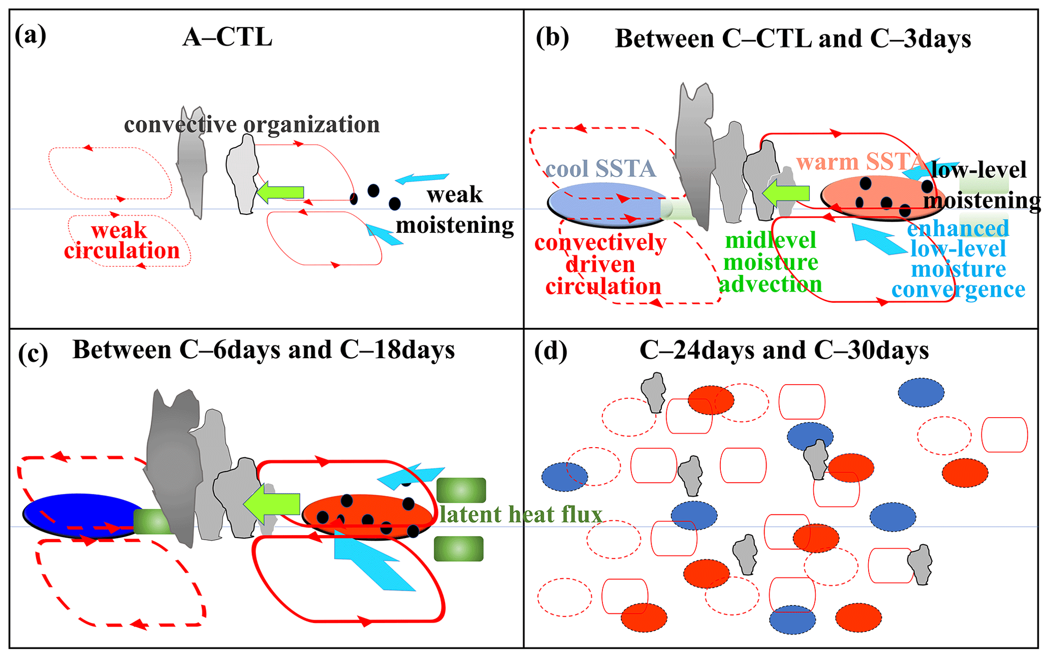
Figure 13 Schematic diagrams illustrate the anomalous circulation and moistening processes during the eastward propagation of the MJO in experiments: (a) A–CTL, (b) high-frequency SST feedback experiments (C–CTL, C–1day, and C–3days), (c) low-frequency SST feedback experiments (C–6days, C–12days, and C–18days), and (d) C–24days and C–30days experiments. In each panel, the horizontal line represents the Equator. The size of clustering gray clouds indicates the strength of convective organization. A red ellipse indicates convection-driven circulation. In the coupled simulations, light red (blue) filled ovals represent warm (cold) SST anomalies, respectively, and grass green rectangles represent latent heat flux. Unresolved convective processes are indicated by black dots representing low-level moisture convergence. Low-level moisture convergence into the equatorial trough is shown by light blue arrows, while mid-level moisture advection is represented by left-pointing green arrows. The deeper colors or thicker lines on the map indicate stronger anomalies in the MJO perturbations. Note that the concept of the figure is based on DeMott et al. (2014).

Finally, results of intraseasonal SST feedback experiments on MJO are summarized schematically in Fig. 13, following DeMott et al. (2014). These experiments included the uncoupled experiment (A–CTL), high-frequency SST experiments (C–CTL, C–1day, and C–3days), low-frequency SST experiments (C–6days, C–12days, and C–18days), and extremely low-frequency experiment (C–24days and C–30days). In the absence of intraseasonal SST variability, the eastward propagation of the MJO was disrupted, leading to weakened or fragmented MJO activity as shown in Fig. 13a. On the other hand, the high-frequency SST experiments closely mimicked air–sea interaction and captured well the characteristics of the MJO. The time-varying SSTs in the coupled simulation provided a certain degree of organization and sufficient surface fluxes, which facilitated the development of the MJO circulation as illustrated in Fig. 13b. The horizontal moist static energy tendency derived from increased low-level convergence, especially due to the meridional advection of MSE, intensified the MJO convection and triggered the eastward propagation over the MC region. The planetary boundary layer (PBL) convergence ahead of the MJO convection is due to kelvin-wave dynamics (Jiang, 2017) in conjunction with the background zonal flow structure (Tulich and Kiladis, 2021). Horizontal MSE or moisture advection in the lower troposphere, particularly the seasonal mean low-level MSE influenced by the MJO's anomalous winds, has had a significant impact on the MJO propagation. (Gonzalez and Jiang, 2017; Jiang, 2017). This simulation result is consistent with the understanding that the MJO is primarily attributed to the interaction between organized convection and large-scale circulation that triggers the eastward propagation. As feedback frequency becomes lower, the major characteristics of the MJO could still be simulated as depicted in Fig. 13c, but with overestimated amplitudes and deteriorating simulations in spatial structures. In the extremely low-frequency experiments with frequency decreasing to 1 per 24 and 1 per 30 d, unorganized structures started to emerge and broke up into smaller-scale perturbations as shown in Fig. 13d, when large-scale air–sea interaction embedded in the MJO did not operate properly in the model. Eventually in the C–30days experiment, unrealistically and spatially scattered anomalies in precipitation, jumping SST, surface heat fluxes, and vertical as well as horizontal MSE advection became dominant features. All these findings led to the major conclusion of this study: more spontaneous atmosphere–ocean interaction (e.g., ocean response once every time step to every 3 d in this study) with high vertical resolution in the ocean model is a key to the realistic simulation of the MJO and should be properly implemented in climate models.