the Creative Commons Attribution 4.0 License.
the Creative Commons Attribution 4.0 License.
 | 14 May 2024
DEUCE v1.0: a neural network for probabilistic precipitation nowcasting with aleatoric and epistemic uncertainties
Seppo Pulkkinen
Terhi Mäkinen
Precipitation nowcasting (forecasting locally for 0–6 h) serves both public security and industries, facilitating the mitigation of losses incurred due to, e.g., flash floods and is usually done by predicting weather radar echoes, which provide better performance than numerical weather prediction (NWP) at that scale. Probabilistic nowcasts are especially useful as they provide a desirable framework for operational decision-making. Many extrapolation-based statistical nowcasting methods exist, but they all suffer from a limited ability to capture the nonlinear growth and decay of precipitation, leading to a recent paradigm shift towards deep-learning methods which are more capable of representing these patterns.
Despite its potential advantages, the application of deep learning in probabilistic nowcasting has only recently started to be explored. Here we develop a novel probabilistic precipitation nowcasting method, based on Bayesian neural networks with variational inference and the U-Net architecture, named DEUCE. The method estimates the total predictive uncertainty in the precipitation by combining estimates of the epistemic (knowledge-related and reducible) and heteroscedastic aleatoric (data-dependent and irreducible) uncertainties, using them to produce an ensemble of development scenarios for the following 60 min.
DEUCE is trained and verified using Finnish Meteorological Institute radar composites compared to established classical models. Our model is found to produce both skillful and reliable probabilistic nowcasts based on various evaluation criteria. It improves the receiver operating characteristic (ROC) area under the curve scores 1 %–5 % over STEPS and LINDA-P baselines and comes close to the best-performer STEPS on a continuous ranked probability score (CRPS) metric. The reliability of DEUCE is demonstrated with, e.g., having the lowest expected calibration error at 20 and 25 dBZ reflectivity thresholds and coming second at 35 dBZ. On the other hand, the deterministic performance of ensemble means is found to be worse than that of extrapolation and LINDA-D baselines. Last, the composition of the predictive uncertainty is analyzed and described, with the conclusion that aleatoric uncertainty is more significant and informative than epistemic uncertainty in the DEUCE model.
- Article
(23937 KB) - Full-text XML
- BibTeX
- EndNote


Predicting the amount and location of precipitation at local scales of a few kilometers for lead times ranging from minutes to hours, i.e., precipitation nowcasting, has recently grown into an important component of severe weather early-warning systems, particularly for those focused on predicting flash floods. Because of the intensification coupled with the increased frequency of extreme precipitation events brought by climate change, accurate estimates of future precipitation have increased in importance. However, the capacity of any nowcasting model to produce accurate estimates is limited and thus also having an idea of the reliability of the nowcast is operationally important. This can be addressed with ensemble nowcasts, which generate a set of possible scenarios, with which it is possible to estimate the probability of certain events.
Numerical weather prediction (NWP) is widely used for forecasts at longer timescales and with coarser grids (Bauer et al., 2015), with regional high-resolution models model generally having a grid resolution of a few kilometers and a refresh rate of typically 1 h. For example, the High-Resolution Rapid Refresh (HRRR) model developed by the United States' National Oceanic and Atmospheric Administration (NOAA) has a grid resolution of 3 km and a refresh rate of 1 h (Alexander et al., 2020). However, NWP does not achieve sufficient performance at the spatiotemporal scales typical of nowcasts, due to not yet having achieved numerical stability in these first few hours and due to the computational complexity of resolving atmospheric equations at sub-hour temporal resolutions and grid resolutions approaching the microscale (≤ 1 km) (Sun et al., 2014; Radhakrishnan and Chandrasekar, 2020). Specialized nowcasting methods for precipitation have been developed in parallel with NWP and may be used in order to circumvent its problems in the domain. These mainly rely on forecasting the evolution of radar echo image sequences that act as a good proxy for ground-level precipitation and usually have a spatial resolution of ∼ 1 km and a temporal resolution of ∼ 5 min, which are characteristic of weather radar observations.
1.1 Extrapolation-based precipitation nowcasting
The most important class of precipitation nowcasting models is based on the extrapolation of radar echoes along the background advection field. These models first estimate the advection field from a sequence of past radar images with methods such as variational echo tracking (Laroche and Zawadzki, 1995) or optical-flow-based methods like the Lucas–Kanade method (Lucas and Kanade, 1981; Bouguet, 2001). In the classical case of the pure extrapolation nowcast, the most recently observed frame is simply extrapolated along the estimated advection field, often using a semi-Lagrangian scheme (Staniforth and Côté, 1991). Extrapolation nowcasting does not model the growth and decay of precipitation, so many extensions attempting to make up for that have been developed. One important method is Spectral Prognosis (S-PROG) by Seed (2003). S-PROG is based on the scale-dependence of the lifetime and evolution of features, decomposing the field into additive components corresponding to different spatial scales and evolving each of them separately using an autoregressive (AR2) model in Lagrangian (flow frame of reference) coordinates, enabling modeling the scale-dependent behavior of precipitation.
STEPS (Short-Term Ensemble Prediction System) by Bowler et al. (2006), is an influential ensemble nowcasting model based on S-PROG. In STEPS, stochastic perturbations are added to the motion field in order to model its uncertainty. Just like with S-PROG, the growth and decay of the precipitation field is modeled by decomposing it using a cascade of scales with the autoregressive model applied to each of these scales separately in Lagrangian coordinates. Unlike in S-PROG, stochastic noise is injected at each scale, concurrent with the AR modeling. Over time, various models have expanded upon STEPS; one recent example is LINDA (Lagrangian INtegro-Difference equation model with autoregression) (Pulkkinen et al., 2021), which uses an integro-difference equation model with rain cell detection and convolutions for modeling the loss of predictability at small scales. LINDA produces nowcasts that are particularly well-suited to the prediction of strong localized rainfall.
1.2 Deep-learning approaches to precipitation nowcasting
With significant recent advances in deep learning, the interest in its use for precipitation nowcasting has increased. One of the first deep-learning models to have been used explicitly for precipitation nowcasting is the convolutional LSTM (ConvLSTM) model (Shi et al., 2015), which combines the temporal prediction capacity of the long short-term memory (LSTM) neural networks with 3D convolutions modeling spatiotemporal features in one model for spatiotemporal nowcasting. ConvLSTM has later been improved by the TrajGRU model (Shi et al., 2017) that replaces the heavy LSTM structure with a lighter GRU (gated recurrent unit) structure and is capable of learning an active location variant structure for the recurrent connections.
Apart from doing the temporal modeling using recurrent units, a popular approach has been to use fully convolutional neural networks, often two-dimensional, thus avoiding the modeling of explicit temporal dependencies. These networks have often been based on U-Net-type architectures, one early example of which is the model by Agrawal et al. (2019), which predicts the exceedance of rainfall over three distinct intensity thresholds for a 1 h lead time. A more useful model is RainNet by Ayzel et al. (2020). RainNet nowcasts rainfall continuously, one time step at a time, inserting the predicted frames back into the network in order to make multiple lead time predictions. Similarly, FureNET by Pan et al. (2021) nowcasts rainfall 1 h at a time using polarimetric input variables, in addition to observed rain rates, via multiple encoder branches and late fusion in the decoder of a residual U-Net architecture and brings improvement compared to using plain rain rates.
The principal problem of using the above deep-learning models for deterministic precipitation nowcasting is that of the increasing blurring of nowcasts with lead time. This is the natural consequence of attempting to minimize the pixel-wise forecasting error in the presence of uncertainties inherent to the task of predicting precipitation. Such loss functions thus behave in the same fashion as S-PROG and STEPS by explicitly filtering out scales through their loss of predictability. One way to resolve the problem is to use generative modeling, which is the approach taken by Ravuri et al. (2021) with their Deep Generative Model of Radar (DGMR). DGMR is an adversarially trained convolutional gated recurrent unit (ConvGRU)-based generative model capable of generating realistic time series of future radar observations that outperform both classical and deep-learning baseline models. In addition to deterministic nowcasts, DGMR is also capable of making ensemble-based probabilistic nowcasts.
Making probabilistic precipitation nowcasts using deep learning has been explored less often than deterministic nowcasts, despite the clear benefit of the probabilistic approach in operational use. In addition to DGMR, other existing probabilistic models are MetNet (Sønderby et al., 2020) and its successor MetNet-2 (Espeholt et al., 2022). MetNet aggregates weather radar, satellite, and orographic information over a large area to predict a probability distribution of rain rate per pixel in one forward pass for a single lead time, with an architecture consisting of a spatial aggregator of inputs, a ConvLSTM spatial encoder, and a spatial decoder with axial attention. The model is shown to outperform the HRRR NWP model on an F1 metric for lead times up to 8 h. MetNet-2 improves upon its predecessor by adding the data assimilation context as an input and aggregating data over a larger area. This enables it to outperform, or at worst rival, HRRR and HREF (High-Resolution Ensemble Forecast) models in continuous ranked probability score (CRPS) and critical success index (CSI) metrics for lead times up to 12 h.
1.3 Uncertainty quantification and Bayesian deep learning
In addition to playing an important role in precipitation nowcasting, the importance of uncertainty quantification (UQ) has also been recognized in deep learning (Abdar et al., 2021). In the field of machine learning, uncertainty in the predictions can be divided into two separate components: epistemic and aleatoric uncertainty. Epistemic uncertainty represents the lack of knowledge in the model, and it is reducible through improving the model or bringing in more training data. Aleatoric uncertainty, on the other hand, is inherent to the input data, and no amount of additional training data or model improvement will reduce it. Aleatoric uncertainty that varies over the input data is said to be heteroscedastic; a constant uncertainty is called homoscedastic.
Many approaches to the quantification of uncertainty have been developed on the deep-learning side. One particularly important theme driving the development in this realm has been operational safety and countering overconfident predictions made by black box models overfitting the training data. Bayesian neural networks (BNNs) have emerged as a candidate for addressing that issue. They work by placing probability distributions over the weights, which are estimated via the means of Bayesian inference and yield a predictive distribution for data through their marginalization.
Although exact Bayesian inference is intractable for large neural networks, suitable approximations exist. These are commonly divided into Markov chain Monte Carlo (MCMC)- and variational inference (VI)-based methods (Jospin et al., 2022). MCMC methods predict better weight distributions but are more computationally expensive and thus often reserved for small-scale problems where performance is key. VI, on the other hand, is more scalable and has been applied to larger neural networks. The idea behind variational inference is to approximate the true posterior of weights with a simpler analytic one (the variational posterior) and to estimate the variational posterior which is the closest to the true one. Thanks to advances by Graves (2011) and subsequently Blundell et al. (2015) with the Bayes by Backprop (BBB) algorithm, it is now possible to use mini-batch optimization for mean field VI (i.e., assuming fully factorizable variational posteriors) on large networks, opening up possibilities for the use of VI in problems such as precipitation nowcasting that require large amounts of input data and numerous model parameters.
Later, Monte Carlo Dropout (Gal and Ghahramani, 2016) techniques, among other variants, have been identified as being equivalent to approximate Bayesian inference due to losing some model expressivity but gaining ease of implementation. Based on this, Kendall and Gal (2017) have developed a technique for estimating the epistemic and heteroscedastic aleatoric variance components separately in deep-learning regression tasks. They estimate the epistemic uncertainty with the variance of predictions made via Monte Carlo Dropout and add a separate component to their network for predicting the aleatoric component. The predictions are modeled as having Gaussian likelihoods, with means equal to the prediction point estimates and variances equal to the aleatoric term described. These terms are then learned by minimizing a Gaussian negative log-likelihood loss function and taking them and observations as inputs. This approach has recently started to be applied to problems such as the segmentation of satellite images (Dechesne et al., 2021), remaining useful for life prognostics (Caceres et al., 2021) and long-term synoptic-scale precipitation forecasts (Xu et al., 2022).
1.4 Model idea and research questions
We propose the Deep Ensemble-based Uncertainty Combining radar Echo nowcasting (DEUCE) model for probabilistic precipitation nowcasting. The idea of the model is to apply the aleatoric and epistemic decomposition of uncertainty by Kendall and Gal (2017) to a Bayesian convolutional neural network with mean field variational inference to produce a predictive distribution of radar reflectivity. This distribution is then sampled to generate ensemble nowcasts of weather radar echo images. The research questions that we will attempt to answer are the following:
-
Can we produce both powerful and reliable ensemble precipitation nowcasts using Bayesian neural networks with uncertainty decomposition? Specifically, is such a model competitive when compared to classical baseline models when assessed with a variety of quantitative probabilistic prediction skill metrics and based on a qualitative assessment?
-
What are the characteristics of the aleatoric/epistemic decomposition? We are interested in the evolution of uncertainties with prediction lead time and whether they capture different and complementary features of the total predictive uncertainty.
-
Can the model additionally be useful in producing deterministic precipitation nowcasts by means of averaging multiple predictions and leveraging the regulatory effect of probability distributions placed on weights? Do such predictions perform competitively when assessed against classical baseline models using quantitative verification metrics? Also, what can those metrics tell us about the nature of the predictions?
DEUCE builds upon a U-Net-based convolutional neural network (CNN) model of deterministic precipitation nowcasting and turns it into a Bayesian neural network with variational inference for making the predictions stochastic, enabling us to model the uncertainty in this U-Net model. As mentioned, we build upon the work of Kendall and Gal (2017) for quantifying the uncertainty in the nowcasting task. Particularly, DEUCE attempts to decompose predictive uncertainty into aleatoric uncertainty (originating from data and irreducible) and epistemic uncertainty (induced by lacking knowledge and reducible) by predicting reflectivity fields along with the aleatoric uncertainty associated with them explicitly. Epistemic uncertainty, in turn, is estimated from the variance in the reflectivity fields sampled, and it is combined with aleatoric uncertainty at the inference time in order to yield an approximation of the total predictive uncertainty. From this point onward, symbols in bold will refer to quantities represented by multidimensional arrays which we interchangeably call tensors. Scalar quantities will be represented with non-bold symbols.
2.1 Functional model
A neural network is a universal function approximator which can be used for regression tasks, mapping an input tensor x to a predicted output tensor and approximating a ground-truth output tensor y, using its learned network parameters θ that are represented as a list of tensors. In the case of radar-based precipitation nowcasting with neural networks, we approximate a function mapping the spatiotemporal time series of past radar observation images , where Lin corresponds to the number of input time steps and to future radar observation images , where Lout corresponds to the number of output time steps. In the DEUCE model, both x and y represent processed radar reflectivity data, and the network outputs a tuple of predicted reflectivity field time series , along with fields estimating the aleatoric uncertainties corresponding to each of the pixels of .

Figure 1The DEUCE encoder and decoder architectural components depicted on the left, along with the architectural diagram making use of those components on the right. Feature maps at different scales are extracted in the encoder branch before being passed to decoder branches, providing the outputs of the network.
For the task of precipitation nowcasting, the neural network has to be capable of outputting predictions for multiple lead times, i.e., discrete time steps in the future, corresponding to future radar observations. DEUCE achieves this using a variant of U-Net as its functional architecture, taking in a sequence of 12 radar reflectivity fields x, predicting that corresponds to the nowcast for the next 12 time steps in a single forward pass.
A schematic representation of the main components of DEUCE and how they are connected is presented in Fig. 1. The architecture consists of a single encoder branch, extracting features from x at different spatial scales and semantic levels. The feature maps from these different scales are preserved for later use through skip connections. The (largest-scale) latent state produced by the encoder and the intermediate feature maps mediated by skip connections are then fed to two independent decoders: one outputting and the other outputting . Using separate decoders for the outputs is preferable over a single combined decoder to avoid the blending of adjacent features, which would be detrimental to the expressivity of the model.
The network contains two-dimensional (spatial) convolutions. These are represented by conv2d 3x3 and conv2d 1x1 labels denoting layers with filter sizes 3 and 1, respectively. Using 2D convolutions, temporal dependencies are only present implicitly. This approximation casts the nowcasting task as a simple image sequence-to-sequence translation problem, which reduces the computational resources needed compared to explicit modeling of the temporal aspect. The convolutional layers use partial convolutions (Liu et al., 2018) in which missing values are masked, and only valid values are used to normalize the convolutions. Although we do not work with missing data, this design choice helps in providing better-quality predictions near image borders by reducing, e.g., various artifacts related to them. ReLU denotes the rectified linear unit activation function, concat is concatenation along the channel dimension, upsample is nearest-neighbor upsampling by a scale of 2, and Max Pooling is maximum pooling by a scale of 2.
2.2 Stochastic model
Conventional neural networks are deterministic in their nature, meaning that they only ever yield the same output for a given input x and parameters θ. Our goal is to produce a reliable estimate of the uncertainty associated with the approximation produced by the neural network. Because this approximation is merely a function of the input data and the functional model including parameters, considering the uncertainty in these sources separately should allow the approximation of the total predictive uncertainty in nowcasts.
Hence, epistemic uncertainty is modeled by placing probability distributions on functional model parameters θ, effectively turning the model stochastic. A Bayesian approach is taken in this regard, placing a prior distribution upon the weights and estimating the most likely posterior distribution given that prior and the training data. The estimation of the true posterior is an intractable task for a large-scale neural network, which is why variational inference (VI) is used to learn approximate posterior estimates for weights. VI limits the space of acceptable posterior distributions to a parameterized family, whose learned parameters replace the point estimates of classical neural network weights. Here, we aim to minimize the Kullback–Leibler (KL) divergence (Kullback and Leibler, 1951) DKL between the true and variational posteriors, which is a measure of the similarity between two probability distributions. As such, the objective is stated as
where θ denotes the variational posterior parameters, θ* the optimal parameters, w the sampled network weights, the problem data, q(w∣θ) the variational posterior, and p(w∣𝒟) the exact posterior of network weights. In practice, this is not directly solvable, so the optimization is accomplished through the maximization of an evidence lower-bound (ELBO) proxy objective. The objective is defined as
consisting of the log-likelihood, log-prior, and log-posteriors, with the last two terms commonly grouped together as the complexity term. Here Eq(w∣θ) denotes the expected value of the probability density of interest over the variational posteriors.
According to Blundell et al. (2015), in Bayesian neural networks and using mini-batch optimization, the ELBO objective, as stated in Eq. (3), can be approximated as
which acts as an unbiased Monte Carlo estimator of the ELBO and is our final loss function. Here, the cost is calculated for each ith of the M mini-batches in an epoch drawing N Monte Carlo samples of the variational posteriors of the weights each time. πi denotes an arbitrary weighting of the complexity term, using the same rule as in Blundell et al. (2015) in this work, which is . This serves to make the regularization effect of the prior stronger earlier, allowing data to be more important later in the training. In DEUCE, the variational posterior distributions q are modeled as diagonal Gaussian distributions, and the Bayes By Backprop (BBB) algorithm, using the re-parameterization trick by Blundell et al. (2015), is employed for their optimization. The prior distribution p(w), on the contrary, is fixed as a hyperparameter and is identically and independently distributed for each parameter as a normal distribution with zero mean and a variance of 0.1. This allows us to potentially calculate the complexity cost in closed form (Hershey and Olsen, 2007), rather than with the Monte Carlo estimate of Eq. (4), hence reducing the computational cost of training.
The likelihood cost of Eq. (4), similar to Kendall and Gal (2017), is modeled for the ith mini-batch and the nth Monte Carlo sample as the Gaussian log likelihood
where the cost is averaged over p=1…P pixels of the spatiotemporal time series s, y and . Lout refers to the length of the time series, W refers to the width of the images, and H refers to the height of the images. i and n indices of fields are omitted here for clarity. Here, y denotes the observed reflectivity fields, denotes the predicted reflectivity fields using the nth weights sampled from the network, and s:=log σ2 refers to the corresponding logarithm of the aleatoric variances predicted by the network with those weights. The logarithm of the aleatoric variances estimate is taken because optimizing using it is more computationally stable and was found to work better than simply using variance constrained to be positive with a ReLU output activation function, especially when dealing with variances approaching zero.
2.3 Generation of ensemble nowcasts
The procedure for producing the primary outputs of DEUCE to make probabilistic nowcasts is presented in Fig. 2. First, N raw network outputs are produced, which are stochastic pairs of reflectivity field sequences and logarithmic aleatoric variance field sequences σn. Each nth of those sampled outputs draws different weights from the learned variational posterior distributions, which is reflected in the output distribution. The σn are converted to their non-logarithmic version , and individual stochastic runs are stacked into a pair of raw ensembles . At this point, the epistemic uncertainty is embedded in , but the aleatoric uncertainty is separate and only present in . Hence, in order to allow the combination of these uncertainties, is divided into the prediction mean and the epistemic variance by taking the mean and variance over , respectively. Additionally, the aleatoric variance σ2 is summarized by taking its mean, denoted . These three outputs, , , and , form the base from which probabilistic nowcasts are computed.
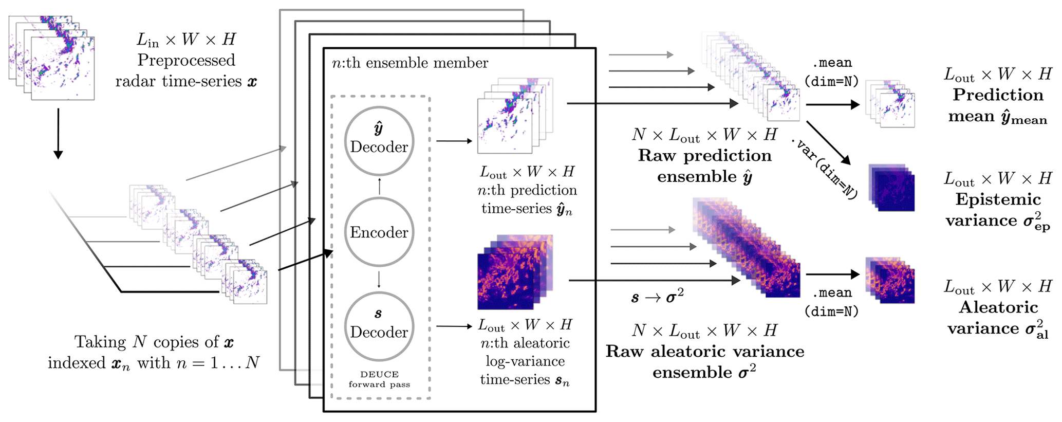
Figure 2The prediction procedure for the primary outputs of the DEUCE is model illustrated. Each sampled output is computed separately with a forward pass through the network, yielding a time series of the predictions and the logarithmic aleatoric variances, which are converted back to variances. After agglomeration into a pair of raw ensembles, the prediction mean and the two types of uncertainties, the epistemic variances and aleatoric variances , are computed from the pair. These three quantities are the ones used for producing the final prediction ensemble.
The total mean and uncertainty in the prediction can thus be estimated as
where denotes the predictive variance. This means that the predictive variance can be estimated as the sum of the variance of the predicted reflectivity fields, which is the epistemic variance, and of the mean of the predicted aleatoric variance fields. These quantities are sufficient for making probabilistic nowcasts such as calculating exceedance probabilities for future radar reflectivity values, allowing us to model the predictive distribution of this reflectivity as normally distributed with mean and variance . This formulation is admissible, as reflectivity of precipitation (in dBZ units) is known to have a normal distribution which follows from the distribution of the precipitation rate being log-normal (Kedem and Chiu, 1987). Additionally, it is interesting to note that the relationship between the ensemble and the predictive distribution here is opposite to that of NWP, where perturbations to initial conditions lead to ensembles that themselves define the predictive distribution (Bauer et al., 2015).
Nevertheless, some applications of probabilistic precipitation nowcasting – such as flood modeling – assume ensemble-based nowcasts, where each member of the ensemble represents a physically plausible precipitation scenario. One could of course randomly sample the predictive distribution to generate an ensemble, which would correctly approximate pixel-wise statistics, but the spatiotemporal structure of the fields would be lost. In an attempt to remedy this, we post-process outputs to generate ensemble members respecting the spatial covariance structure of the input field x as
where denotes the newly generated ensemble member, ⊗ denotes an element-wise multiplication broadcast over Lout frames, and ϵcorr,n is a correlated Gaussian random field of shape W×H. ϵcorr,n is generated to match the average spatial correlation structure of x using fast Fourier transform (FFT) filtering. The structure is obtained non-parametrically from the power spectrum of x (Seed et al., 2013). The technique is equivalent to that used to generate perturbation fields in STEPS (Pulkkinen et al., 2019). Even though this method accounts for the spatial structure of the precipitation time series, it is not capable of modeling its temporal structure, which is assumed constant. The ensembles produced in this way shall be denoted , which is in contrast to the raw predicted reflectivity fields denoted .
This section presents the experiments performed. First, in Sect. 3.1, we present the dataset used, followed by the details related to the training of DEUCE in Sect. 3.2, and the verification experiments in Sect. 3.3. Additional technical details can, on the other hand, be found in Appendix A.
3.1 Data
The dataset used for this work comes from the Finnish Meteorological Institute radar network. It consists of cropped lowest-altitude radar reflectivity composites chosen from rainy days during the summer period of the years 2019–2021. The dataset is identical to that used by Ritvanen et al. (2023), except for using longer time series. The composites are built from the two lowest-elevation angle scans interpolated into an 1×1 km Cartesian grid. The chosen area covers southern Finland, with the bottom-left corner at coordinates (59.01° N, 20.55° E) and the top-right corner at coordinates (63.62° N, 30.27° E). The spatial extent of this crop is 512×512 km, corresponding to 512×512 pixel square images, suitable for training a neural network. The composites are available with a temporal resolution of 5 min. The extent of the bounding box is additionally illustrated in Fig. 3, along with the coverage of Finnish Meteorological Institute radars. From this we see that the advantage of the crop is that it has a higher-density radar cover than its surroundings.
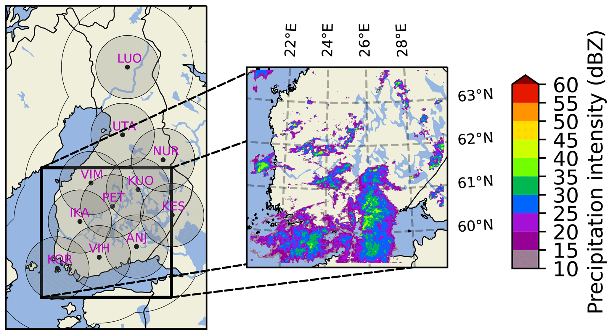
Figure 3The Finnish Meteorological Institute radar network with its 11 radars and the bounding box used. Each radar is described by its three-letter code, with their 120 km coverage radii for snowfall in gray and the intersection of 250 km coverage radii for rainfall as the black outline. An example radar composite crop from a precipitation event (15 August 2019 at 15:00:00 UTC) is visualized in the enlarged version of the bounding box on the right.
The data were selected on a day-by-day basis, selecting the 100 d with the most pixels having reflectivity values over 35 dBZ. The days were then divided into 6 h long blocks from which blocks with below 1 % of the pixels with reflectivity values over 20 dBZ were removed. These remaining blocks were then randomly split into training, validation, and verification datasets with a ratio of . The division into blocks was done in order to limit the number of successive time series present in different splits, as they exhibit high correlation, and not using any blocks would make the training, validation, and verification sets dependent, as the same events would be present in all of them. A time of 6 h was deemed a sufficient time for temporal correlations to mostly disappear. Last, 2 h long time series, corresponding to 24 images each, were then extracted from these blocks using a sliding window principle, with a stride of one, omitting those time series with missing data. The final training, validation, and verification datasets ended up containing 10 780, 1813, and 1666 time series, respectively.
The input time series were read from HDF5 files, stored there with an 8 bit scale-offset lossy compression scheme, ranging from −32 to 96 dBZ at a resolution of 0.5 dBZ. The images were then converted to floating point values, and a threshold of 8 dBZ was applied, replacing values below the threshold with −10 dBZ. This served as a simple way to remove non-meteorological targets and other clutter that could interfere with the training and prediction while maintaining most of the relevant precipitation echoes. Finally, the reflectivity values were normalized between zero and one. Computed predictions were converted back into reflectivity values by applying the inverse of the transformation before saving them, using the same scheme as with the input data.
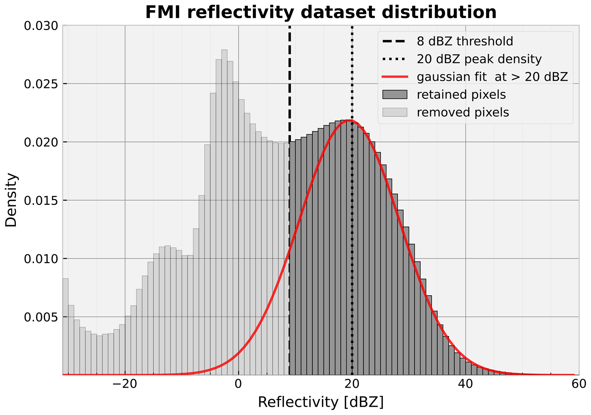
Figure 4Finnish Meteorological Institute composite crop dataset distribution of reflectivity. The threshold chosen below which the data are set to −10 dBZ is shown with a dashed line. Additionally, a Gaussian probability density function (PDF) fit on the data above 20 dBZ is shown in red, which serves to illustrate the Gaussian distribution of precipitation reflectivity.
The dataset reflectivity distribution is depicted in Fig. 4, with the −32 dBZ minimum value pixels left out of the histogram for clarity. The threshold is shown to divide the data into retained and discarded parts, and a Gaussian density is fitted to the part most likely to purely consist of precipitation, which exceeds 20 dBZ. Below the threshold, there seem to be multiple peaks in density, likely involving insects, birds, and miscellaneous clutter, as well as increasing noise the lower we go on the scale. While the highest-reflectivity density values seem to follow the Gaussian fit well, part of the density between 10 and 20 dBZ remains unexplained, and this range is likely to contain a mixture of precipitation and clutter. Still, this is not a major issue, since the most interesting precipitation to predict corresponds to reflectivity values well above 20 dBZ.
3.2 Training
For the training of the network, the Adam optimizer (Kingma and Ba, 2015) was used with an initial learning rate of and other parameters set to their PyTorch default values. The network was trained with that learning rate for 20 epochs, after which the learning rate was lowered to for 8 more epochs, and finally further lowered to for 1 final epoch. A validation epoch was carried out after each epoch in which equitable threat score (ETS) (Hogan et al., 2010) metrics were calculated for converted precipitation estimates (Sect. A1) of predictions and summed over thresholds of 0.5, 1.0, 5.0, 10.0, 20.0, and 30.0 mm h−1, as well as each lead time. This validation score showed improvement over the whole training process.
The training procedure for DEUCE is presented in Fig. 5 for a single epoch. Both input sequence lengths Lin and output sequence lengths Lout were 12, corresponding to 1 h each. For the training and validation epochs, the batch size was set to two, and the number of produced Monte Carlo samples of posteriors N was set to two as well, which was the most that our GPU could fit during training. In order to increase the variance between the gradients of mini-batch members, Flipout re-parameterization (Wen et al., 2018) was applied to the sampled weights, multiplying the random sampling coefficient of weights with a random sign matrix and effectively adding randomness inside batches for a low computational cost. The closed-form of the KL divergence between two Gaussian distributions was used for the calculations of the ELBO complexity term instead of Monte Carlo estimates in the final model training.
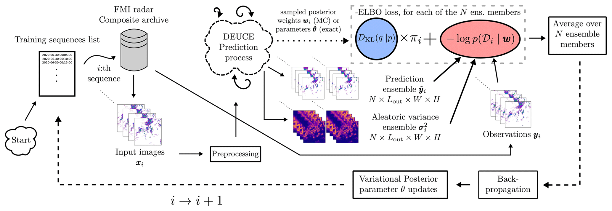
Figure 5An illustrated training epoch for DEUCE. One loop corresponds to a single training sequence, which can be substituted for a single training mini-batch, taking multiple sequences in one batch. The DEUCE prediction process refers to that illustrated in Fig. 2, without the post-processing. The blue box labeled DKL(q‖p) corresponds to the complexity term of the negative ELBO loss (to minimize), πi corresponds to its weighting coefficient, and the red box labeled corresponds to the likelihood term of the negative ELBO loss. Monte Carlo estimates of the complexity term use sampled weights wi, whereas the closed-form expression that we use is a function of parameters θ.
The input time series Xi was pre-processed first, as described in Sect. 3.1, and, in the case of training data, was then augmented by applying in succession a random horizontal flip, a random vertical flip, and a rotation by an angle randomly chosen between 0, 90, 180, and 270°. This was done to improve the variety in the training dataset and consequently improve the generalization performance of the trained network.
3.3 Verification
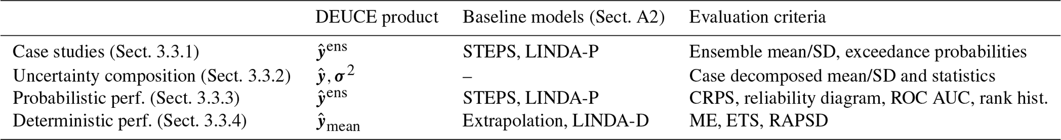
The performance of the DEUCE model is verified against the pySTEPS (Pulkkinen et al., 2019) implementation of multiple extrapolation-based precipitation methods. The verification is divided into the qualitative inspection of ensembles produced in two case studies, into an analysis of DEUCE uncertainty composition, into the verification of the (probabilistic) performance of the whole ensemble, and into the verification of the (deterministic) performance of the ensemble mean, i.e., its fidelity in representing the true variation in the radar images. The four types of verification performed, along with the relevant DEUCE product, the baseline models used, and the evaluation criteria are summarized in Table 1.
Table 1The four components of the verification process for DEUCE summarized.
In probabilistic verification experiments, N=48 ensemble members are used both for producing the raw outputs and for drawing the post-processed ensemble , as well as for making the baseline ensemble model predictions. All of the predictions made for the verification of DEUCE are made until a 60 min lead time and thresholded at 8 dBZ, serving as an estimate for minimum observable precipitation. Four precipitation thresholds are considered where the verification involves evaluating the quality of a prediction exceeding a particular reflectivity value. Converted using the Z–R relationship presented in Sect. A1, these are 20 dBZ (≈0.5 mm h−1), 25 dBZ (≈1.3 mm h−1), 35 dBZ (≈5.7 mm h−1), and 45 dBZ (≈25.5 mm h−1), which correspond to very light, light, moderate, and heavy rain, respectively.
3.3.1 Case studies
Two distinct rainfall events are chosen as case studies to provide a qualitative assessment, as well as a comparison of DEUCE nowcasts with the baseline probabilistic methods. The case studies each focus on an ensemble nowcast at a particular time step during the precipitation event that is chosen to include both large-scale weaker precipitation, which is characteristic of stratiform rainfall, or localized heavy precipitation, which is characteristic of convective rainfall. The latter has a shorter lifetime and has been traditionally harder to predict, but it is of interest to observe the performance of the model with both types. In addition, we include both instances of weakening and of intensification of echoes in the case studies. The cases are chosen from radar composite crops, with the area described in Sect. 3.1 over the verification split, and the summer of the year 2022, which is separate from the dataset used for training, validation, and quantitative verification. The timestamp of the first case chosen is 9 July 2022 at 15:00:00 UTC. This case contains mostly convective rainfall, with some localized high rain rates. The second case chosen is 17 August 2021 at 16:50:00 UTC, which represents a very different scenario with large-scale, mostly stratiform rainfall. The radar images of the hour leading up to the timestamps are used as inputs and the following 1 h of radar images are predicted.
Three different visualizations of the cases are made at 5, 15, 30, and 60 min lead times, using the post-processed DEUCE ensembles and the probabilistic baseline models STEPS and LINDA-P described in Sect. A2 when appropriate. The first visualization is that of predictive means and standard deviations of the ensembles (in dBZ units). Here, DEUCE, STEPS, and LINDA-P are compared side by side. The second visualization is that of exceedance probabilities of DEUCE, STEPS, and LINDA-P ensemble nowcasts at a 25 dBZ reflectivity threshold. The third, and last, visualization depicts the exceedance probability of DEUCE in predicting reflectivity above 20, 25, 35, and 45 dBZ thresholds.
3.3.2 Uncertainty composition analysis
The composition of the DEUCE predictive uncertainty is analyzed using the prediction of the first case study and using statistics aggregated over the verification dataset. For the case study prediction, the aleatoric and epistemic components of the predictive standard deviation are visualized next to the combined predictive uncertainty, the mean predictions, and the observations at lead times of 5, 15, 30, and 60 min. The statistics collected are the average magnitude of the aleatoric and epistemic standard deviation components under different conditions. These magnitudes are divided into bins corresponding to the prediction lead time and the observed reflectivity matching the pixel in question (5 dBZ bin width from 5 to 60 dBZ) and are collected for each prediction timestamp. The resulting statistics are visualized in the form of a histogram aggregated over the whole dataset and as bar plots showing the contribution of the uncertainties against lead time and observed reflectivity.
3.3.3 Probabilistic performance verification
Probabilistic verification serves to assess the probabilistic predictive power of DEUCE ensembles, mostly in terms of prediction reliability and discrimination ability. In other words, it determines the quality and the variety of produced ensembles with regard to the true distribution of different future scenarios. Here, the DEUCE prediction is represented by the post-processed ensemble . The probabilistic baseline models used are STEPS (Bowler et al., 2006; Seed et al., 2013) and LINDA-P (Pulkkinen et al., 2021). The description and configuration of those models are given in Sect. A2.
The probabilistic performance metrics used are the continuous ranked probability score (CRPS) (Hersbach, 2000; Wilks, 2011), which generalizes the mean absolute error in deterministic forecasts to probability distributions and is calculated for lead times up to 60 min. Next, the receiver operating characteristic (ROC) curve (Mason, 1982; Wilks, 2011), along with the area under it (AUC), quantifies the discriminative power of the ensembles for predicting reflectivity values exceeding a certain threshold. ROC AUC is computed for reflectivity thresholds of 20, 25, 35, and 45 dBZ at lead times of 5, 15, 30, and 60 min. To measure forecast reliability and sharpness, we used the reliability diagram, along with its sharpness histogram (Wilks, 2011), and the expected calibration error (ECE) score (Naeini et al., 2015), which we computed for the same threshold and lead times as ROC curves. Finally, rank histograms (Wilks, 2011) were calculated to measure the bias and spread of ensembles at lead times of 5, 15, 30, and 60 min. A detailed description of these metrics, along with the configurations used, is found in Sect. A3.
3.3.4 Deterministic performance verification
Deterministic verification serves to assess whether DEUCE ensemble means are useful themselves. It also gives insight into many interesting aspects of predictions, such as systematic biases and the possible loss of small-scale variability. Here, the DEUCE prediction is represented by the ensemble mean . The deterministic baselines used are an extrapolation nowcast and LINDA-D (Pulkkinen et al., 2021). The description and configuration of those models are again described in Sect. A2.
Three deterministic metrics are used to assess DEUCE ensemble means. The first is the mean error (ME) (Wilks, 2011), measuring the bias of nowcasts produced. The equitable threat score (ETS) (Hogan et al., 2010; Wilks, 2011) then provides an estimate of the deterministic skill in forecasting reflectivity above a certain intensity threshold. It is calculated for lead times up to 60 min and thresholds of 20, 25, 35, and 45 dBZ. Finally, the radially averaged power spectral density (RAPSD) (Ruzanski and Chandrasekar, 2011; Ulichney, 1988) measures how well the power spectrum of reflectivity is maintained. It is summarized with a relative mean absolute error (MAE) score. We compute RAPSD for prediction lead times of 5, 15, 30, and 60 min. RAPSD is also calculated for individual members to analyze the possible contribution of the spatially correlated noise to maintaining the power spectrum. A detailed description of these metrics, along with the configurations used, is found in Sect. A4.
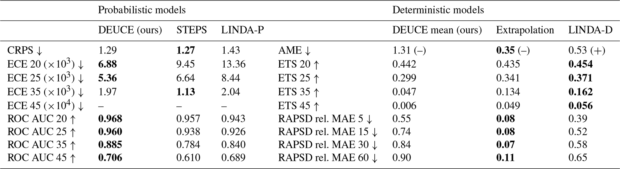
The results of the quantitative and qualitative analyses of model performance and fitness to the task indicate that DEUCE succeeds in its primary task of providing reasonably reliable probabilistic precipitation nowcasts but not in that of producing skillful deterministic nowcasts. This is illustrated by the summary of quantitative verification results is provided in Table 2. These results will then be elaborated upon in detail and presented as figures in the following four subsections. Starting with the qualitative case study results in Sect. 4.1, we then present the composition of the uncertainty in Sect. 4.2, before continuing with the probabilistic performance metric results in Sect. 4.3, and finally presenting the deterministic performance metric results in Sect. 4.4.
Table 2Quantitative verification metrics are summarized. The ↑ indicates that a higher score is better, while the ↓ indicates that a lower score is better. The best score amongst models is marked using bold font. ECE scores indicate the expected calibration error, which is an aggregate measure of reliability. AME stands for absolute mean error, and RAPSD rel. MAE score summary values indicate the relative mean absolute error between the power spectral density (PSD) of the observation and predictions. For AME, the sign of the mean error is reported in parentheses. Scores are averaged over the lead times for which they were calculated, except for RAPSD rel. MAE scores, as they are averaged over frequencies. Numerical values in the ECE, ROC AUC, and ETS score names indicate decibels relative to Z threshold values and in RAPSD lead time in minutes. ECE 45 results are omitted because the results are not comparable due to missing data in some of the bins of the DEUCE reliability diagrams.
4.1 Case studies
The results of the first case study in Figs. 6, 7, and 8 suggest that DEUCE ensemble nowcasts are able to give reasonable uncertainty and exceedance probability estimates at multiple thresholds and lead times and that DEUCE nowcasts look similar to those given by STEPS, despite being less grainy. The results of the second case study are detailed in Appendix B. Figure C1 shows an example of what individual ensemble members look like at different prediction lead times for the first case. The predictions all start out being quite similar, but they eventually diverge, driven by the increasing predictive uncertainty and different patterns of correlated noise. The ensemble members exhibit variety while preserving a moderate amount of realism that is nevertheless limited by the increasing smoothing of the predictive mean and variance fields with lead time.
4.1.1 Ensemble mean and breadth
Ensemble mean and breadth as units of standard deviation are shown for the first case in Fig. 6. Here, we can see a trend in all models towards a loss of predicted reflectivity intensity and a disappearance of heavily localized echoes. However, these are in all models compensated by an increase in the spatial extent and the magnitude of the ensemble standard deviation. In LINDA-P, the effect of predicting in rain rate (mm h−1) is seen as the uncertainty in the cell borders emphasized. LINDA-P also generally exhibits a smaller and more uniform standard deviation than the other models. For a 1 h lead time, DEUCE seems to generally have an ensemble breadth a bit smaller than STEPS but higher than LINDA-P, with the most heterogeneity in the standard deviation values.
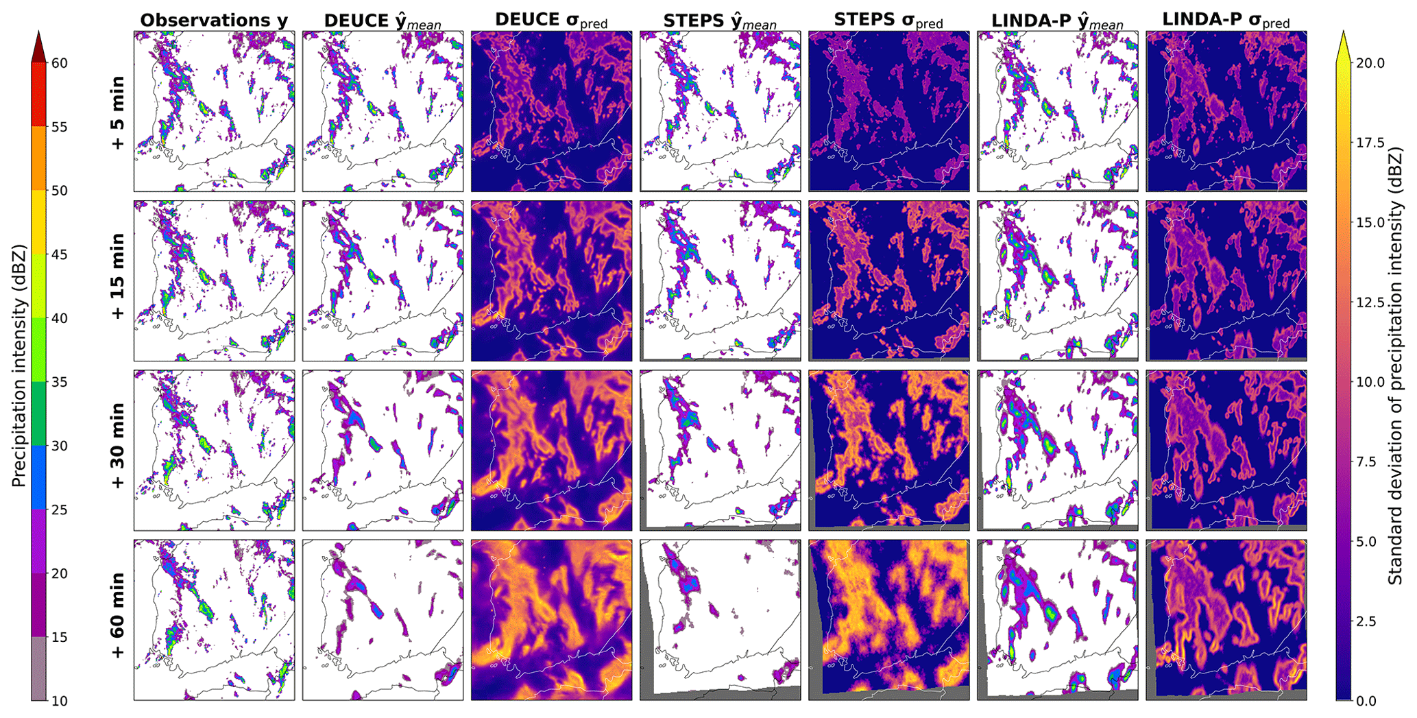
Figure 6The first case study ensemble means and breadths of DEUCE compared to STEPS and LINDA-P model predictions and observations for multiple lead times. The area covers southern Finland, starting at 15:00:00 UTC on 9 July 2022. The rows represent lead time and columns different instances of observations, model mean, and standard deviations. Missing values are indicated by a dark gray color.
4.1.2 Reflectivity exceedance probabilities
Reflectivity probabilities of exceeding 25 dBZ predicted by the different models for the first case are shown in Fig. 7. Overall, DEUCE seems to provide balanced exceedance probabilities that are not missing any significant areas even after 1 h but are also not covering excessively large areas. Comparatively, STEPS tends to completely miss some significant portions, such as in the area highlighted in the southwest of Finland at 1 h, and generally seems to predict smaller probabilities for the evolution of smaller cells. LINDA-P, on the other hand, suffers from overconfidence and misplaces the evolution of multiple precipitation areas after 1 h. On a general level for all models compared, the advection field is well captured, while the growth and decay of echoes are often not very effectively forecast. The anisotropic structure of the uncertainty shown through exceedance probabilities is also much better captured by DEUCE and LINDA-P than STEPS. In addition, because it is not based on the extrapolation of radar echoes, there are no “dead zones” filled with NaN (not a number) values (dark gray color), and DEUCE is able to provide nowcasts with varying success in border regions where STEPS and LINDA-P predictions are not necessarily defined.
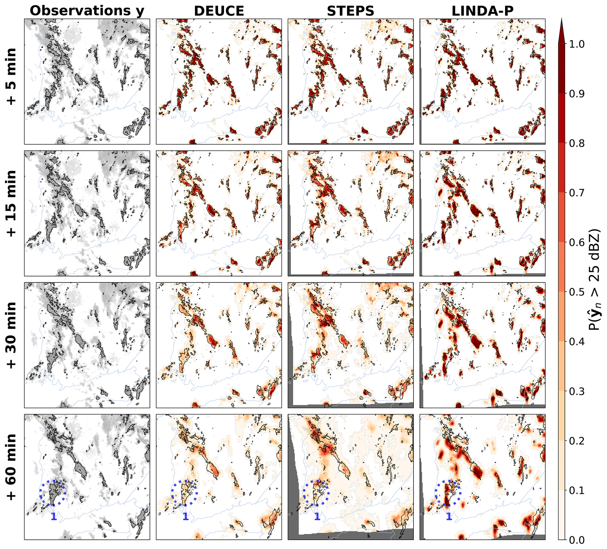
Figure 7The first case study reflectivity exceedance probabilities of 25 dBZ for DEUCE compared to STEPS and LINDA-P model predictions and observations for multiple lead times. The area covers southern Finland, starting at 15:00:00 UTC on 9 July 2022. The rows represent the lead time. In the leftmost column, actual observations are shown in light gray, with echo isotherms corresponding to the threshold marked in black. In other columns, the same isotherms are overlaid on the exceedance probabilities of the models that are depicted in shades of red. Missing values are indicated by a dark gray color. The blue circles labeled “1” highlight a case of DEUCE model improvement over baselines.
Last, the exceedance probabilities of DEUCE nowcasts for 15, 25, 35, and 45 dBZ reflectivity thresholds for the first case are shown in Fig. 8. We can see that DEUCE is able to nowcast an exceedance probability at all thresholds (which are indeed all exceeded at some place and point in the observations). Higher thresholds exhibit lower values and some misplacement of exceedance probabilities, as precipitation exceeding those is more difficult to predict and has smaller areas.
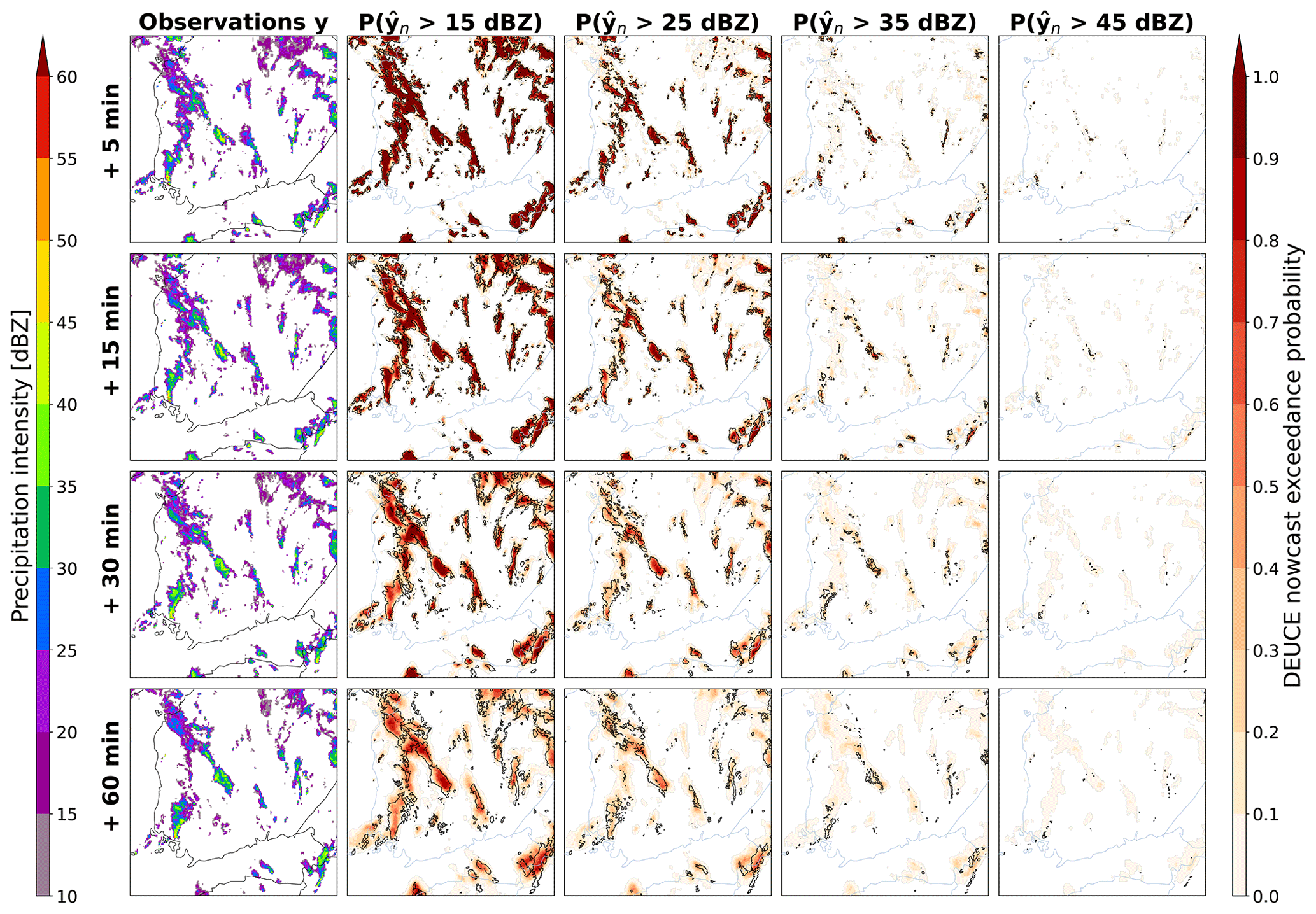
Figure 8The first case study reflectivity exceedance probabilities of DEUCE compared to observations for multiple lead times and reflectivity thresholds. The area covers southern Finland, starting at 15:00:00 UTC on 9 July 2022. The rows represent lead time. The leftmost column is observations, and the rest are exceedance probabilities at different thresholds. As in Fig. 7, the observation isotherms corresponding to the threshold in question overlay the exceedance probabilities depicted in shades of red.
4.2 Analysis of the aleatoric and epistemic uncertainty dichotomy
The relative contribution of aleatoric and epistemic uncertainty for the first case study is presented in Fig. 9. We can see that most of the predictive uncertainty in fact comes from the aleatoric part. Epistemic uncertainty is of much smaller magnitude, and its contribution is further reduced when working in terms of variance in the calculation of predictive uncertainty. We can see that epistemic uncertainty does not extend as much away from the core of the predicted reflectivity as for aleatoric uncertainty, which reflects a small variance in the raw ensemble. This overlap can be seen in probabilistic nowcasts as aleatoric uncertainty overshadowing the contribution of epistemic uncertainty.
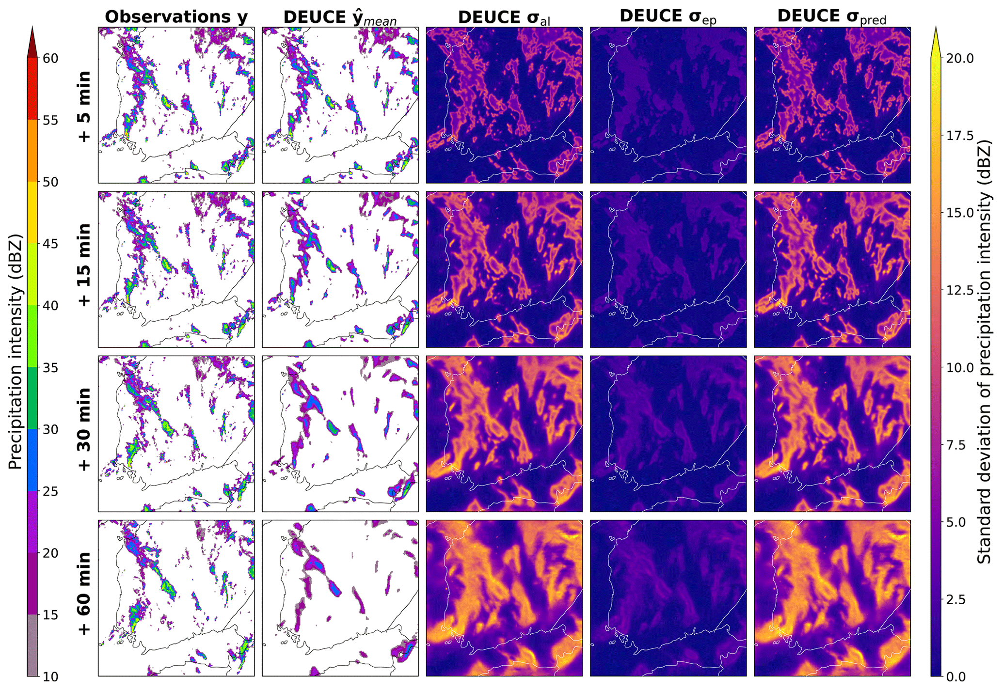
Figure 9Composition of the predictive uncertainty for the first case study. The area covers southern Finland, starting at 15:00:00 UTC on 9 July 2022. The rows represent lead time and columns observations (ground truth), the mean prediction, aleatoric and epistemic standard deviation components, and the combined predictive standard deviation.
A more detailed view of the contribution of aleatoric and epistemic components is provided in Fig. 10, with statistics over the whole verification dataset. A histogram of the uncertainties aggregated over all lead times and observed reflectivity values is shown to the left of Fig. 10. Epistemic uncertainty has a very narrow distribution, mostly between 0–5 dBZ, which means that its average value could not have varied much in different cases, lead times, and observed reflectivity values, pointing to a small model uncertainty response to these factors. Aleatoric uncertainty, on the other hand, has a long-tail distribution centered around 10 dBZ but going up to values over 30 dBZ, which means that we cannot exclude a dependence on these external factors.
Such dependencies are confirmed when inspecting the bar plots on the right of Fig. 10, where mean aleatoric uncertainty shows a clear dependence on prediction lead time and to some degree on observed reflectivity. Aleatoric uncertainty seems to clearly increase with lead time and to first slightly decrease before increasing again in relation to observed reflectivity. One possible explanation for this last observation is that reflectivity values below 20 dBZ often correspond to the edges of precipitation cells, which are difficult to predict, and that reflectivity values over 35 dBZ often correspond to heavy precipitation with a short lifetime and thus bad predictability. In between those, there are more predictable precipitation patterns, such as the interior of stratiform precipitation cells. Epistemic uncertainty, on the other hand, does not seem to show any particular dependence on prediction lead time, which might have something to do with the fact that the model predicts all lead times at once, making it possibly more difficult for the predictions to vary, depending on the lead time. There is, on the other hand, a slight increase in the epistemic uncertainty with observed reflectivity, which might be an accurate reflection of the relatively smaller amount of training data available for high observed reflectivity values.
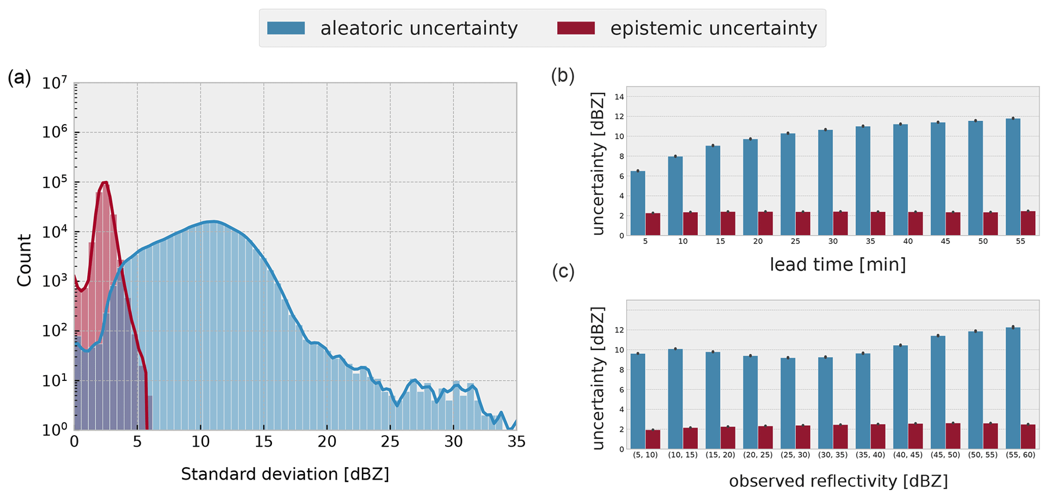
Figure 10Visualization of the statistics on the composition of predictive uncertainty over the verification dataset. On the left, a histogram of aleatoric and epistemic standard deviation (SD) aggregated over all lead times and observed reflectivity values is shown. On the right, we arrange the same data into bar plots to show the relationship between the type of the uncertainty SD with prediction lead time (b) and observed ground truth radar reflectivity (c).
4.3 Probabilistic skill verification
The reliability diagrams and sharpness histograms for probabilistic nowcasts are depicted in Fig. 11. It can first be noted that, in general, DEUCE nowcasts are very close to the dashed black line, indicating a perfectly reliable forecast. Sometimes, this is similar to baseline models, but in some cases, such as a long lead time and a high threshold, DEUCE is closer to the diagonal than baselines. This is, however, not reflected in the ECE scores at 35 dBZ shown in Table 2, as smaller forecast probabilities are weighted much higher due to their sample count here, making STEPS the most reliable model at 35 dBZ when using this metric. An important pattern is that compared to baseline models, DEUCE is prone to slight under-forecasting of the exceedance probabilities. This is particularly the case for a short lead time (5 min), where the effect is the most pronounced. As lead times grow longer and thresholds get higher, nowcasting gets harder, and there is an overall tendency in all models, but particularly LINDA-P, to over-forecast threshold exceedance.
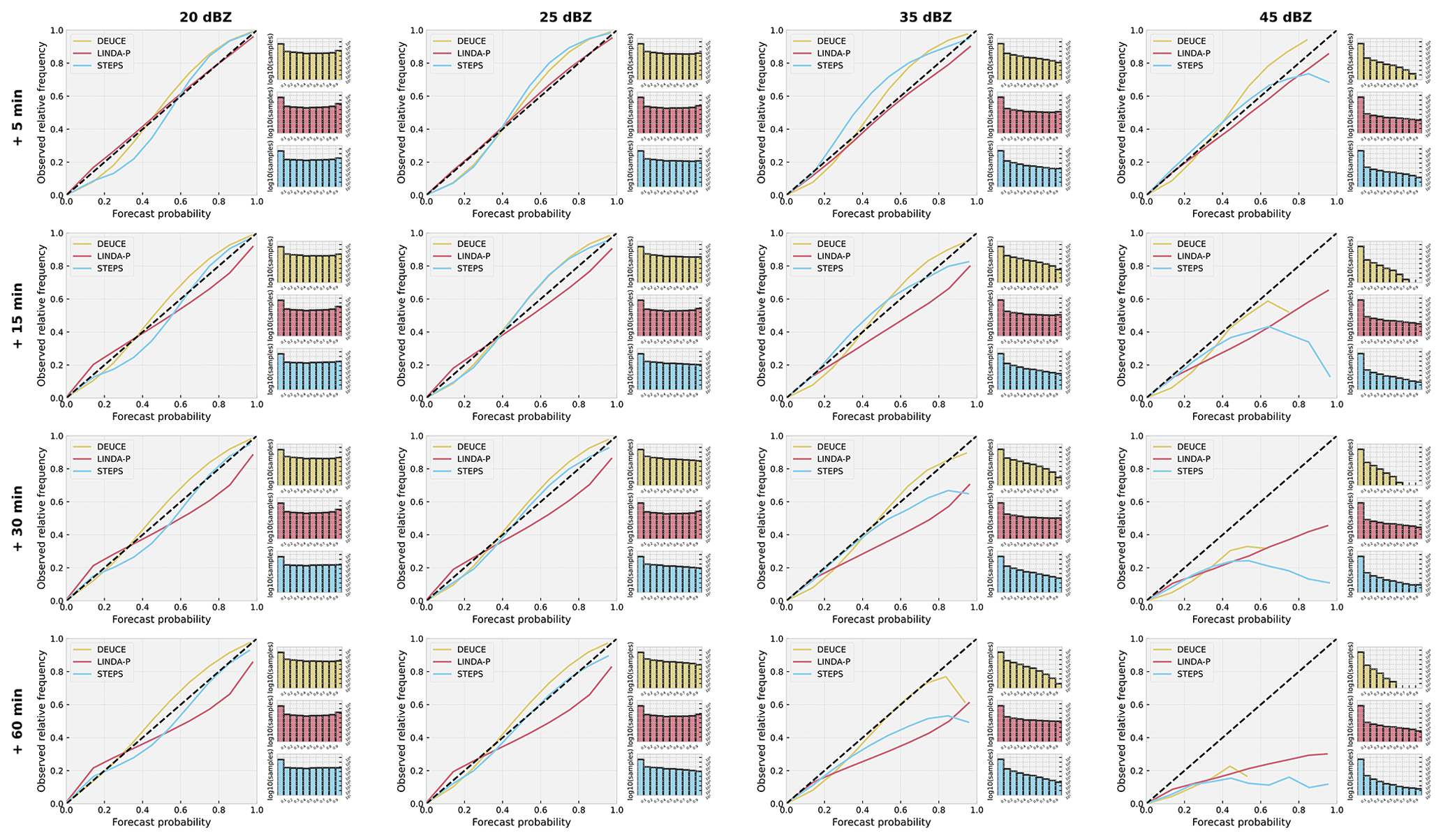
Figure 11The reliability diagrams and sharpness histograms for DEUCE (yellow), STEPS (blue), and LINDA-P (red) model nowcasts at exceedance probability thresholds of 20, 25, 35, and 45 dBZ and at lead times of 5, 15, 30, and 60 min. Rows indicate the lead time and columns the exceedance probability threshold. The diagonal dashed black lines indicate perfect reliability.
From the sharpness histogram, it is seen that the distribution of forecast probabilities is more or less uniform at low thresholds but more biased towards small exceedance probabilities at higher thresholds. These higher thresholds are where the difference between DEUCE and baselines is visible, as there is a considerably lower number of cases of high forecast probability in DEUCE than in baselines.
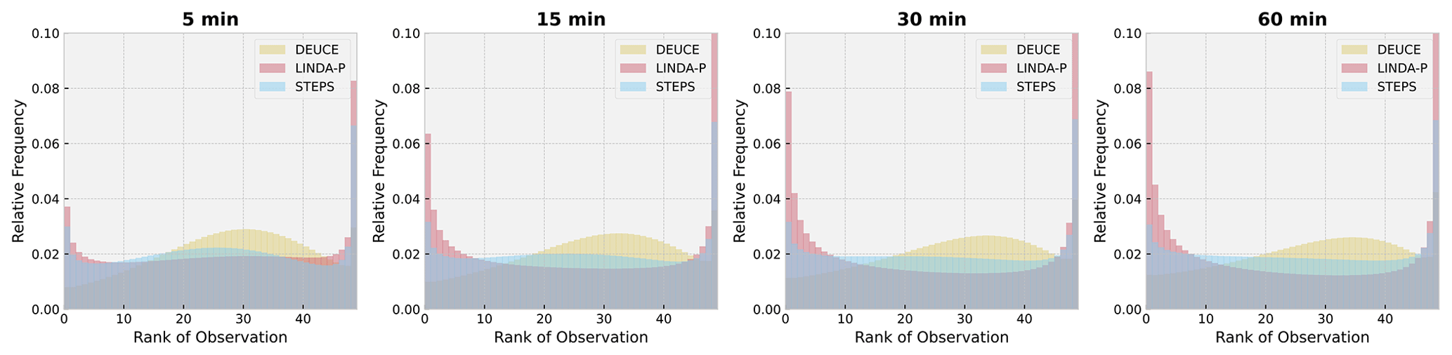
Figure 12Rank histograms of ensemble nowcasts, including DEUCE, STEPS, and LINDA-P, at lead times of 5, 15, 30, and 60 min over the verification set.
The rank histogram of nowcasts is shown in Fig. 12. It is apparent here that DEUCE is constantly slightly biased towards predicting reflectivity values that are too low and that the spread is large at short lead times but less significant later on. STEPS exhibits a very balanced flat histogram, but LINDA, on the other hand, has a U-shaped histogram characteristic of an ensemble breadth that is too small in general.
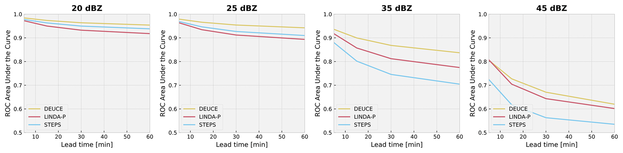
Figure 13The ROC area under the curve (AUC) values at lead times up to 60 min for DEUCE (yellow), STEPS (blue), and LINDA-P (red) model nowcasts at exceedance probability thresholds of 20, 25, 35, and 45 dBZ.
The results for the ROC area under the curve probabilistic nowcast metric are shown in Fig. 13. In this benchmark, DEUCE achieves the best results at all thresholds. We can notice that STEPS has good discriminative power at low thresholds but that it does not scale well to higher ones and that LINDA-P is not competitive at lower thresholds but excels as the threshold grows. Nevertheless, DEUCE manages to perform better than both in their skillful areas.
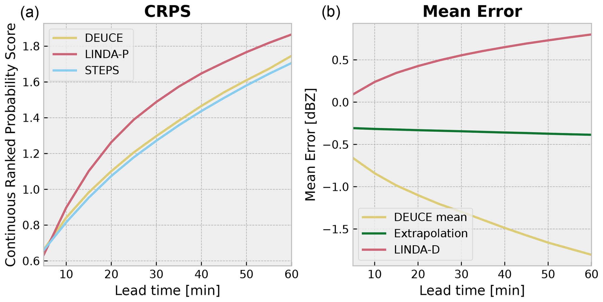
Figure 14The CRPS score of DEUCE (yellow) compared to the ensemble baselines of STEPS (blue) and LINDA-P (red) is shown on the left. The mean error (ME) score for non-augmented ensemble mean predictions of DEUCE (yellow) compared to deterministic baseline extrapolation (green) and LINDA-D (red) nowcasts is shown on the right.
Last, the CRPS verification metric is depicted in Fig. 14. It can be seen that the lowest and best score is achieved by STEPS at all lead times. DEUCE comes second, slightly above STEPS, and LINDA-P lags far behind. Overall, with CRPS, it can be seen that DEUCE achieves adequate results of the order of baseline models.
From the quantitative probabilistic verification, it can be summarized that DEUCE achieves satisfactory and well-rounded performance. The model does not significantly lack in any category in particular and offers a good trade-off between forecast reliability and discriminatory power.
4.4 Deterministic skill verification
Here, we analyze the results of the comparison of the deterministic nowcast skill between DEUCE non-augmented mean predictions and baseline predictions. First, a depiction of the mean nowcasting error (ME) until a 60 min lead time is presented in Fig. 14. While extrapolation nowcasts have, on average, a ME slightly below zero, DEUCE is more strongly negatively biased, while LINDA-D is strongly positively biased.
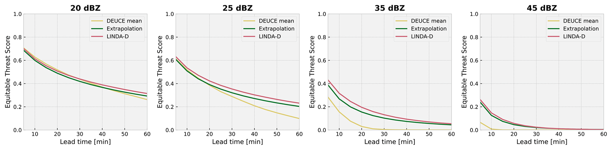
Figure 15Equitable threat scores (ETSs) as a function of lead time for non-augmented DEUCE ensemble means (yellow) compared to those of extrapolation (green) and LINDA-D (red) deterministic baseline models for reflectivity thresholds of 20, 25, 35, and 45 dBZ at lead times up to 60 min. DEUCE ensemble means perform competitively for predicting reflectivity exceeding 20 dBZ but see their relative performance drop at higher reflectivity thresholds.
Furthermore, the equitable threat score (ETS) results for reflectivity thresholds of 20, 25, and 35 dBZ are shown in Fig. 15. The ETS score of DEUCE is competitive for the 20 dBZ threshold, but at 25 dBZ, its progression at lead times longer than 30 min is already worse than the baseline. At 35 and 45 dBZ, DEUCE already performs worse than the baseline at any lead time examined. The reason for this weakness is the compound effect of intrinsic CNN prediction smoothing and the averaging of ensemble members. This smoothing effect is also visible in the radially averaged power spectral density (RAPSD) results for nowcasts presented in Fig. 16. Average RAPSD is computed for nowcasts at lead times of 5, 15, 30, and 60 min. It can clearly be seen that, compared to baselines, the fields predicted by DEUCE lose more power at small spatial scales and that this effect is heavily amplified at longer lead times, which again illustrates the above compound effect. However, this effect seems to be damped by augmenting the mean prediction with uncertainty-weighted correlated noise following the structure of the input field, especially at longer lead times.
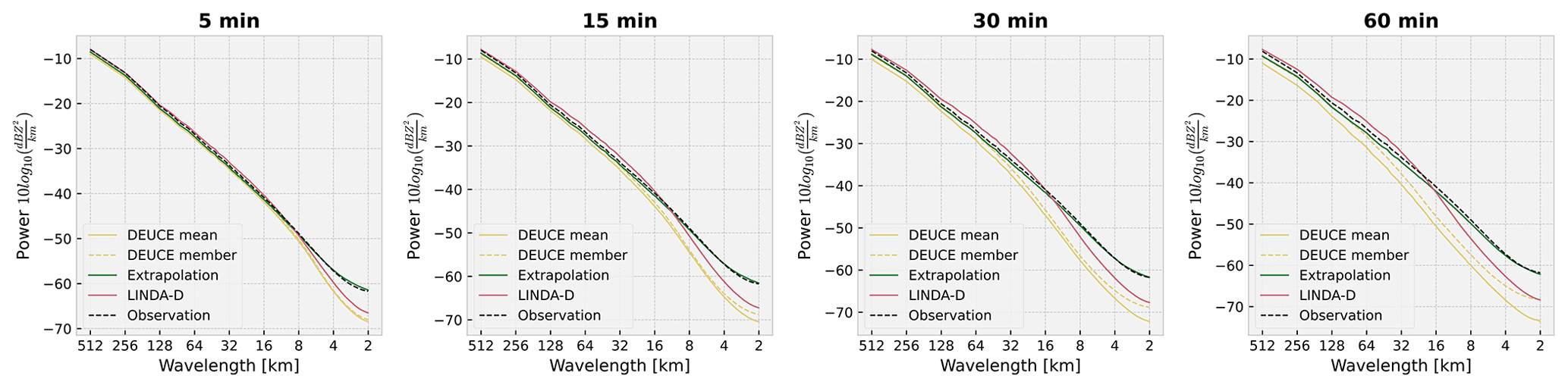
Figure 16Radially averaged power spectral density (RAPSD) for non-augmented DEUCE ensemble means (solid yellow) and individual augmented DEUCE ensemble members (dashed yellow) compared to those of the extrapolation (green) and LINDA-D (red) deterministic baseline models at lead times of 5, 15, 30, and 60 min. The observation RAPSD is shown as a dashed black line.
DEUCE probabilistic ensemble nowcasts proved to be both relatively reliable and skillful compared to STEPS and LINDA. In comparison, STEPS was often reliable but struggled to capture small-scale high reflectivity, and LINDA was better at this task but sometimes suffered from overconfidence. DEUCE seems to offer a good compromise as it does not suffer too much from either of those two defects. Nevertheless when analyzing the reliability diagram, it is apparent that DEUCE is under-confident, especially at short lead times. Further inspection of rank histograms (Fig. 12) – showing the distribution of the rank of observations among ensemble members – indicated that this under-confidence is expressed by (1) an ensemble spread that is too large and (2) a slight bias towards ensembles producing estimates that are too weak, which was also visible in the ensemble mean ME score. The ensemble spread that is too large may be a byproduct of attempting to predict the ensemble mean and aleatoric variances all at once, with the prior placed on weights that place a limit on the complexity of the model and in effect privileging the learning of longer lead times where the average errors are of a bigger magnitude.
We can also observe that most of the uncertainty is of an aleatoric nature and that the contribution of epistemic variance is universally low. In addition to having trained with a large amount of data, low epistemic variance is probably related to the variational inference mechanism, as the combination of Bayes by Backprop and Flipout re-parameterization has been shown by Valdenegro-Toro and Mori (2022) to yield epistemic uncertainty estimates that are too small when compared to Monte Carlo Dropout, deep ensembles, and Markov Chain Monte Carlo. Another factor that might have played a role in this is again predicting all lead times at once because adopting the iterative approach of RainNet (Ayzel et al., 2020) would have propagated previous epistemic uncertainties to subsequent lead times, possibly balancing out the contributions, and also allowing predictions to be made for an arbitrary number of time steps. On the other hand, abandoning the recursive prediction scheme of RainNet significantly reduces the time complexity of computing from 𝒪(NL) to 𝒪(N), where N is the sample size, and L is the number of prediction lead times.
Contrary to the preliminary iteration of the model focusing only on modeling epistemic uncertainty (Harnist, 2022), the current model better captures the increased spread of the predictive distribution with lead time through the aleatoric component. An alternative model – without a separate decoder branch for σ2 and only allocating a separate output channel to it – was not successful because the and σ2 that it learned were highly correlated, more blurry, and lacked expressivity. It is for this reason that the two-branch version was adopted.
In DEUCE, small-scale variability is steadily lost with increasing lead time, which is especially noticeable for lead times over 30 min. This is a problem for the production of realistic nowcasts, as the loss of small-scale variability is synonymous with the loss of information, limiting the expressivity of the model. However, the smoothing of radar image predictions can be justified in the case of a probabilistic model, assuming that the breadth of the ensemble is preserved despite the loss of high frequencies. This is because information will invariably be lost with time as we attempt to predict the evolution of a chaotic system through imperfect measurements. In the present case of DEUCE, the predictive distribution is modeled explicitly, giving us the ability to arbitrarily sample from it, so this loss of high-frequency components is not a major issue. For the preliminary version of the model (Harnist, 2022), however, losing small-scale details had adverse effects. This was because the model was trained with homoscedastic (fixed as a hyperparameter) aleatoric uncertainty modeling, which was not taken into account when making predictions, resulting in an ensemble spread of smooth predictions that is too small and leading to vastly underestimated exceedance probabilities. The spatially correlated noise scheme for sampling the predictive uncertainty may help integrate DEUCE into applications where physically plausible ensemble members are necessary. Still, the lack of temporal correlation modeling inside the post-processed ensemble members and the smoothing of the predictive means and variances themselves limit realism, pointing to the limits of the taken approach. One grounded method for resolving this problem is to either implicitly or explicitly constrain the predictions to replicate the power spectrum of observations. Generative models such as GANs (Generative Adversarial Networks) fall into the category of implicit constraining. For example, the DGMR model by Ravuri et al. (2021) learns to model realistic spatial and temporal correlations by adversarially training the generator with two discriminators designed to discern those aspects.
We see that the issues of under-forecasting at short lead times and lacking small-scale variability could be linked and related to the model training settling for underperforming local optima. Avenues to mitigate this include longer training and different training strategies, using a bigger and more varied dataset, adapting the loss function, and improving the model itself. DEUCE was trained with only 29 epochs, which is a relatively small number. We attempted to train with a higher number of epochs, but this did not result in consistent improvement in model validation performance metrics. However, this behavior might have been related to our choice of learning rate scheduling. On the other hand, it might also be worthwhile to attempt to implement a curriculum learning strategy where easier to learn and earlier lead times would be learned first before allowing the network to learn to predict longer lead times. The dataset size itself may be increased by covering a variety of bounding boxes in the composite area and by including precipitation events from outside the summer period. The likelihood part of the loss function may be adapted so that higher weight is given to higher-reflectivity pixels. We, nevertheless, found this tricky to get right, as the experiments that we performed with weighting proportional to the inverse of the density of the reflectivity in the dataset distribution failed to produce reasonable nowcasts. From the perspective of the model, under-forecasting and the lack of small-scale details could be reduced by including spatial and channel (temporal for us) attention mechanisms, such as the Convolutional Block Attention Module (CBAM) (Woo et al., 2018), which has been applied to improve (deterministic) precipitation nowcasting performance (Trebing et al., 2021). CBAM might enable, for example, sharper forecasts with smaller aleatoric uncertainties at short lead times without affecting the reliability at longer lead times.
It is important to note that all models, DEUCE included, are generally not able to predict convective initiation, which is a notoriously hard problem to solve (Prudden et al., 2020). This is clearly illustrated with the new echoes appearing in the northwestern (continuously) and southern (between 30 and 60 min) parts of the second case (Fig. B2) for which very low exceedance probabilities are predicted. Adding polarimetric or vertical profile information as additional input channels and adopting a model less susceptible to blurring might improve this aspect of predictions.
With regard to the model development in general, some degree of hyperparameter optimization was performed. Those hyperparameters related to the functional model and the optimizer are mainly inherited from RainNet (Ayzel et al., 2020), and those related to variational inference mostly originate from the preliminary version of the model (Harnist, 2022). There, the VI-related parameters specifically demanded non-trivial tuning for model convergence and acceptable result production, which might limit the immediate applicability of the model in its default state. Also, the local optimality of the current hyperparameters is not assured. Despite this, VI and epistemic uncertainty are not decisive factors in the model performance, and swapping out those components is a potential way forward. Moreover, 60 min (12 frames) of input data and the same length for predictions were picked without optimization in an attempt to preserve some symmetry between the network inputs and outputs. Although there is no consensus yet on how many frames are needed, as few as four input frames have be enough to saturate model performance in some conditions (Ravuri et al., 2021), so tuning the ratio of input to output frames could be a viable thing to try.
Regarding the verification process, it is a pertinent question to ask whether the used baseline models were sufficient to validate the performance of DEUCE. In particular, the lack of deep-learning ensemble baselines is one weakness of the performed verification. It would have been particularly interesting to use the Deep Generative Model of Radar (DGMR) by Ravuri et al. (2021) as a baseline, as it represents the current state-of-the-art in deep-learning-based precipitation nowcasting and is capable of producing ensemble nowcasts. Unfortunately, we were not able to successfully train DGMR on our dataset using the resources that we had allocated for the task. Other models of interest that were not included in the verification are MetNet by Sønderby et al. (2020) and its successor MetNet-2 by Espeholt et al. (2022), which use, e.g., orographic and satellite data in addition to radar data. We hope that further work will make the comparison of DEUCE probabilistic nowcasting performance to other deep-learning-based models possible.
One last point of concern regards the validity of the verification metrics used. The potential issues here mostly relate to the summarizing quantitative metrics of Table 2. First, the relative RAPSD MAE metric for measuring the power spectrum fidelity of predictions uses a tighter sampling of points towards wavelengths representing small spatial scales, which biases it to give a higher weight to those scales. Although we are indeed mostly interested in small-scale variations, this property means that even big discrepancies in the power of large spatial scales will be under-represented. Next, the ECE metric used to summarize the reliability of ensemble models is very sensitive to variations of the order of magnitude of the number of samples per bin. This behavior is significant especially at higher exceedance thresholds, where almost all prediction probabilities are concentrated in the smallest probability bin, giving almost no weight to even the mildly successful nowcasting of rare but significant events of high heavy precipitation probability. This means that ECE does not necessarily provide a complete assessment of model reliability in the context of probabilistic precipitation nowcasting.
We developed a probabilistic precipitation nowcasting model named DEUCE, based on a Bayesian neural network with variational inference and featuring the combination of epistemic and aleatoric uncertainty estimates in an attempt to yield reliable yet powerful probabilistic predictions. The model succeeded at this primary task, performing competitively against the baseline STEPS and LINDA-P models that were judged using qualitative and quantitative evaluation.
It was found that DEUCE had issues with the representation of epistemic uncertainty, leading to most of the uncertainty appearing as aleatoric uncertainty, maybe due to the variational inference used. The aleatoric uncertainty exhibited a clear dependence on lead time and corresponding observed reflectivity, which are factors heavily influencing the predictability. The epistemic uncertainty, on the other hand, showed little dependence on these factors, with the exception of a slight increase with observed reflectivity, which might reflect the distribution of the training data. Based on this, aleatoric and epistemic uncertainties do indeed seem to capture complementary features of the predictive uncertainty.
Deterministically, the ensemble means were found to perform worse compared to extrapolation and LINDA-D baselines, showing that the model in its current state is not useful in the deterministic case due to the excessive smoothing of predictions. This smoothing may also have affected the uncertainty composition, such that assuming the predictive mean to be fixed, i.e., with no improvement in skill, means that sharper reflectivity predictions would increase the epistemic uncertainty. As for the aleatoric uncertainty, the variation between individual draws would increase, but their average would not necessarily increase, except for cases where smoothing is the mechanism that hinders the prediction of large enough reflectivity values. In those cases, the average aleatoric uncertainty might decrease. Looking into future research directions, DEUCE has a number of different facets upon which its performance could be improved. First, the underlying U-Net could potentially be replaced by a more powerful architecture capable of modeling explicit temporal dependencies. The spatiotemporal extent could be enlarged, and additional orographic, polarimetric, or satellite input channels could improve parts of the nowcasts. It is possible to additionally try to leverage other patterns for increasing predictability, such as operating in Lagrangian coordinates, as shown by Ritvanen et al. (2023), to increase prediction performance. From a probabilistic aspect, certain alternative inference methods, such as radial Bayesian neural networks (Farquhar et al., 2020) or deep ensembles, look promising as a potential way to ease the training and improve the representation of epistemic uncertainty. We could also think of directly appending the post-processing sampling with spatially correlated noise to the neural network or even learning context-dependent spatiotemporal correlation structures. The sampled outputs could then be, e.g., fed to a GAN-like discriminator module which would drive the processed outputs to be more realistic while retaining the uncertainty decomposition.
Regardless of its shortcomings, DEUCE is a first step in ensemble-based probabilistic precipitation nowcasting using Bayesian neural networks. The concurrent modeling of aleatoric and epistemic uncertainties has the potential to be useful for operational forecasters, and the model in its current state forms a strong yet relatively lightweight baseline for future developments in deep-learning-based probabilistic precipitation nowcasting.
A1 Ground precipitation estimates from reflectivity
The formula was used in cases where an estimate of ground precipitation corresponding to lowest-level radar reflectivity composites was needed. Here R denotes precipitation estimates (in mm h−1), and z denotes radar reflectivity (in dBZ). The parameters of the Z–R relationship employed in the formula come from the work of Leinonen et al. (2012) and aim to estimate the amount of rainfall corresponding to radar reflectivity measurements from the Finnish Meteorological Institute polarimetric C-band radars in Finland.
A2 Baseline models
There are two deterministic baseline models: a simple extrapolation nowcast and the deterministic variant of LINDA (LINDA-D). The extrapolation nowcast extrapolates the last input reflectivity field along a motion field calculated from the last four elements of the input time series. In the extrapolation nowcast and all other baseline methods, we use the dense Lucas–Kanade optical flow method with its default pySTEPS parameters for the computation of the motion field. In addition, all baseline nowcasting methods use the semi-Lagrangian integration scheme from pySTEPS for performing the extrapolation, with cubic interpolation and other parameters left to their default values.
LINDA, a more advanced extrapolation-based method capable of predicting high-intensity rainfall more accurately, serves as a natural benchmark in the deterministic and probabilistic cases for the ability of the model to capture convective rainfall evolution. LINDA predictions are made using reflectivity fields converted to rain rate, using the method described in Sect. A1, as it is required for the model to work. LINDA models here use the last three input rain rate fields as input, in addition to the motion field. They do not use feature detection in order to reduce the prediction computation time over the verification set to more practical durations. The ensemble-producing version of LINDA, LINDA-P, is used as a probabilistic baseline model; while LINDA-D deterministic nowcasts do not add any perturbations, LINDA-P does add them, as well as velocity perturbations from Bowler et al. (2006), with lucaskanade/fmi+mch parameters (Pulkkinen et al., 2019). Other parameters are set to be data-specific or to be their default values.
The STEPS model is used in addition to LINDA-P as a probabilistic baseline. While being a bit older and having lower discriminative power, it is a popular method for making reliable probabilistic precipitation nowcasts to this day. STEPS is applied to decibels relative to Z (dBZ) reflectivity fields and also takes in the last three input images, in addition to the motion field. Field perturbations and motion field perturbations are applied with the same parameters as with LINDA-P. Six cascade levels are used for the cascade decomposition, and the precipitation threshold of 8 dBZ is given as the lowest observable precipitation intensity.
A3 Details on probabilistic verification metrics
A3.1 Continuous ranked probability score (CRPS)
The CRPS generalizes the MAE to probability distributions by calculating the sum of the difference between the cumulative density function (CDF) of the nowcast and the empirical CDF of observations. It is defined as
where denote possible forecast values, denote the forecast CDF, and denote the empirical CDF of observations y.
A3.2 Receiver operating characteristic (ROC) curve
The receiver operating characteristic (ROC) curve (Mason, 1982; Wilks, 2011) quantifies the discriminative power of an ensemble for predicting over a certain threshold by keeping track of the false alarm rate (FAR), i.e.,
where the rate of false positives is indicated by FP, and the rate of true negatives is indicated by TN, and both are compared to the probability of detection (POD), i.e.,
where TP is the rate of true positives, and FN is the rate of false negatives. POD is regularly binned, and FAR is averaged over those bins, making a curve, the area under which (AUC) summarizes the overall discriminative power of the nowcasting method. A ROC AUC of 0.5 indicates zero skill, whereas a value of 1.0 indicates a perfect forecast. For ROC curve computations, we use 10 bins.
A3.3 Reliability diagram
The reliability diagram (Wilks, 2011) measures the reliability of the forecast by presenting the observed relative frequencies of dBZ threshold exceedance events against the forecast probability of those events. Having these two values strongly correlate makes the forecast reliable. Reliability diagrams are built by dividing the forecast probabilities into bins (we choose 10) and incrementing them with associated binary indicators of whether the event happened. Sharpness histograms represent the number of events recorded in each forecast probability bin. They measure the relative “decisiveness” of the forecast, where a high decisiveness is associated with a convex histogram shape. A low decisiveness, on the other hand, can be discerned from a more uniform, or in the extreme case, a concave histogram shape.
A3.4 Expected calibration error (ECE)
The expected calibration error (ECE) (Naeini et al., 2015) quantitatively summarizes the reliability of a model indicated by a reliability diagram. It is defined as
with a total of N pairs of forecast probability and observation, forecast probabilities divided into B bins, with nb observations per bin, fb is the mean bin forecast probability, and ob is the corresponding observation frequency in the bin. ECE corresponds to the MAE of the reliability diagram to the diagonal and is weighted by the number of observations per bin.
A3.5 Rank histogram
Rank histograms (Wilks, 2011) measure the bias and spread of ensemble nowcasts. They present a histogram of the rank of the true observed echo reflectivity among all ensemble members, where a convex histogram indicates a small spread and a concave histogram indicates a small spread. On the other hand, a higher frequency of low ranks for observations indicates a positive bias of predictions, and a higher frequency of high ranks for observations indicates a negative bias of predictions.
A4 Details on deterministic verification metrics
A4.1 Mean error (ME)
The mean error (ME) (Wilks, 2011) measures the bias of deterministic predictions. It is defined as
for images, or time series of them, with P pixels. This metric tells us about the mean bias of nowcasts produced. The absolute value of ME is used to give a quantitative summary of the bias of predictions made.
A4.2 Equitable threat score (ETS)
The equitable threat score (ETS) (Hogan et al., 2010; Wilks, 2011) is an extension of the threat score, also known as the critical success index (Schaefer, 1990). ETS aims to provide an estimate of deterministic skill in forecasting precipitation above a certain intensity threshold. This extension takes into account the effect of randomly occurring true positives. ETS is defined as
where the rnd term estimates the influence of random true positives.
A4.3 Radially averaged power spectrum density (RAPSD)
The radially averaged power spectrum density (RAPSD) (Ruzanski and Chandrasekar, 2011; Ulichney, 1988) measures how well the power spectrum of precipitation is maintained when calculated for nowcasts at different lead times. RAPSD fidelity is summarized as
which is the absolute error between the observed and predicted PSD, relative to observed PSD, averaged over frequencies. Here, F denotes the number of frequencies of the power spectrum, is the power of the observed field at the fth frequency, and is the power of the predicted field at the fth frequency. Taking the relative values allows the comparison of spectral densities on multiple scales. In the present case, PSD frequencies are sampled linearly, weighting corresponding wavelengths towards smaller scales, effectively biasing small-scale errors to be more important. This is, however, not necessarily a problem, as prediction fidelity at small scales is the most important question we seek to answer with RAPSD.
A5 Hardware and software packages used
The DEUCE model was built on PyTorch (version 1.12.1). PyTorch Lightning (version 1.7.7) was used to organize the neural network training and prediction workflow, and the TyXe library (version 0.0.1) was used to turn DEUCE Bayesian, making use of the Pyro (version 1.4.0) probabilistic programming language as its back-end for variational inference. The DEUCE training and prediction were performed using the Finnish IT Center for Science (CSC) supercomputer Puhti, using one NVIDIA V100 GPU with 32 GB of VRAM, 64 GB of RAM, and 10 cores from a 2.1 GHz Intel Xeon Gold 6230 CPU. For the evaluation of the model performance, we used the pySTEPS library (version 1.6.1). It served to produce baseline extrapolation-based model nowcasts, to calculate verification metrics, and to help with their visualization. The pySTEPS-based verification pipeline was run on a computational server of the Finnish Meteorological Institute equipped with two Intel Xeon Gold 6138 2.0 GHz CPUs, each with 20 cores and 2 threads by core, as well as 192 GB of RAM.
The results of the second case study show a similar behavior to that of the first case study (Sect. 4.1) but generally lower uncertainty values, especially on the inside of the areas containing precipitation.
B1 Ensemble mean and breadth
Ensemble mean and breadth as units of standard deviation are shown for the second case in Fig. B1. Here, we observe a generally similar trend, as with the first case (Sect. 4.1), with the difference being that the ensemble breadth of STEPS is only higher than that of DEUCE towards the center of the rainfall areas, as it tends to be similar at the outskirts of those larger areas. Among the different models, we can also observe the most heterogeneity and anisotropy in the predictive distribution of DEUCE.
B2 Reflectivity exceedance probabilities
Reflectivity probabilities of exceeding 25 dBZ predicted by the different models for the second case are depicted in Fig. B2, and many of the same comments can be made with respect to the first case (Sect. 4.1), with DEUCE seeming to offer the best balance between accuracy and lacking too many false positives.
For this second case study, the exceedance probabilities of DEUCE at thresholds of 15, 25, 35, and 45 dBZ are shown in Fig. B3. It is worth pointing out that DEUCE was not able to predict the growth of a substantial new rainfall area in the northwest of the composite, despite the predictive uncertainty being significant there, as shown in Fig. B1, which can be understood because the predictive means under the 8 dBZ threshold were generally closer to the minimum value of −10 dBZ.
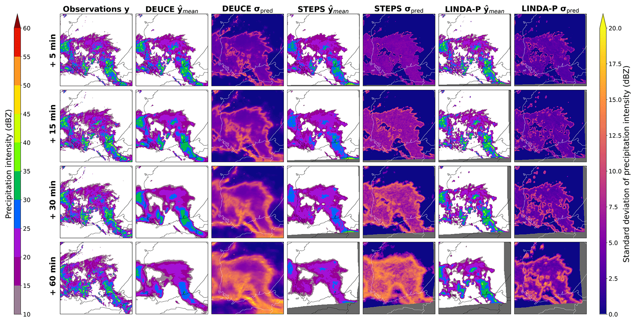
Figure B1The second case study ensemble means and breadths of DEUCE compared to STEPS and LINDA-P model predictions and observations for multiple lead times. The area covers southern Finland, starting at 16:50:00 UTC on 17 August 2021. The rows represent lead time and columns different instances of observations, model mean, and standard deviations. Missing values are indicated by a dark gray color.
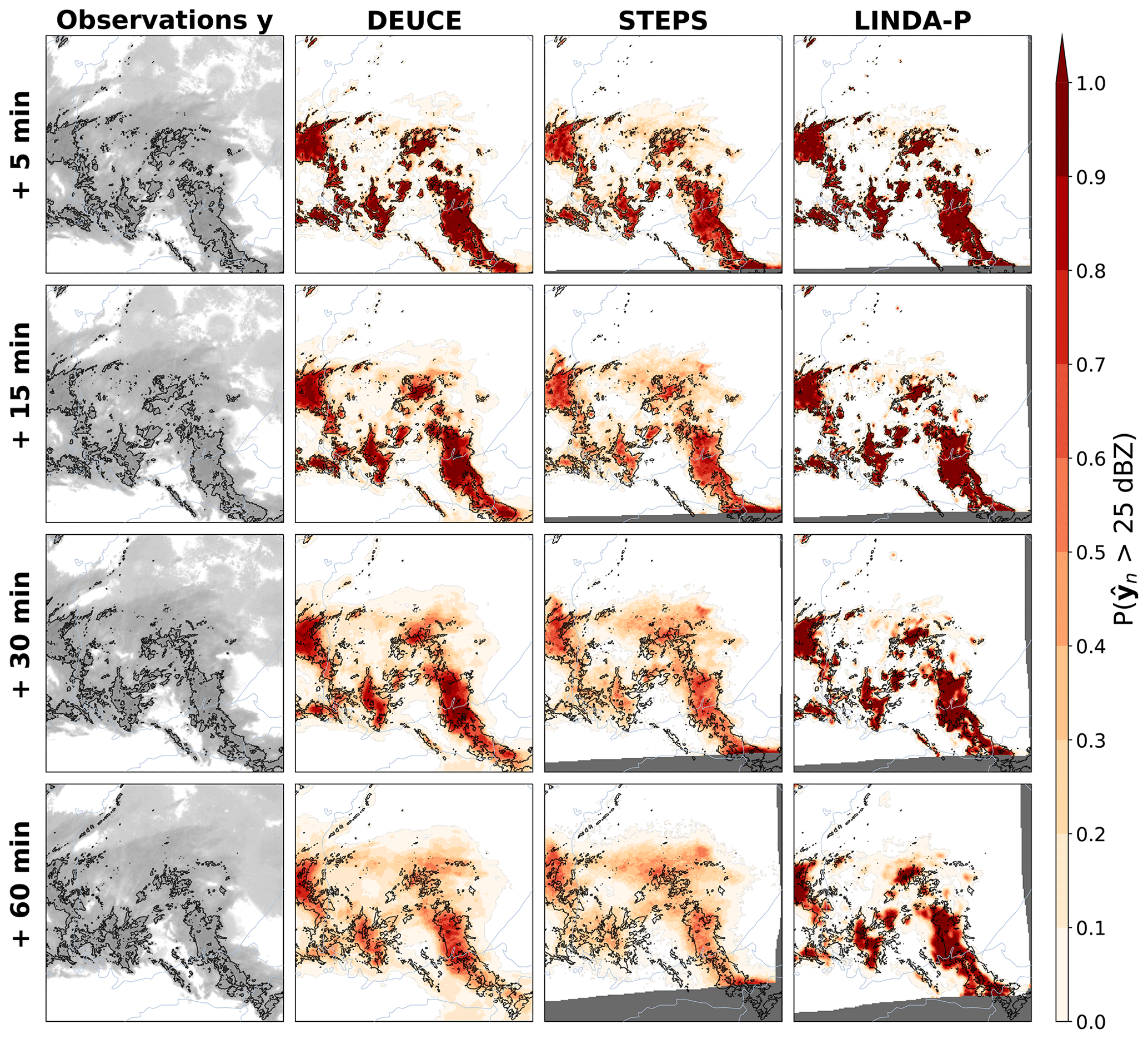
Figure B2The second case study reflectivity exceedance probabilities of 25 dBZ for DEUCE compared to STEPS and LINDA-P model predictions and observations for multiple lead times. The area covers southern Finland, starting at 16:50:00 UTC on 17 August 2021. The rows represent lead time. In the leftmost column, actual observations are shown in light gray, with echo isotherms corresponding to the threshold marked in black. In other columns, the same isotherms are overlaid on the exceedance probabilities of the models and depicted in shades of red. Missing values are indicated by a dark gray color.
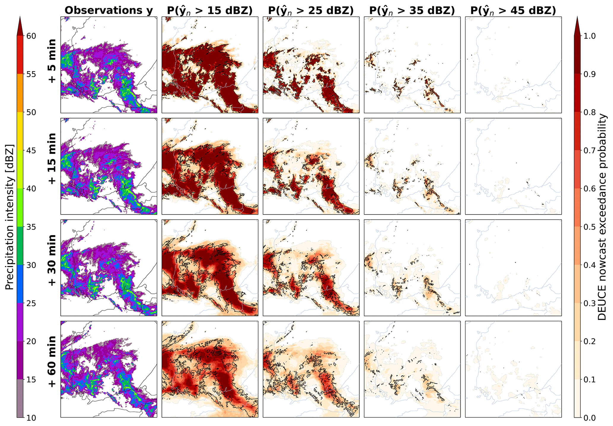
Figure B3The second case study reflectivity exceedance probabilities of DEUCE compared to observations for multiple lead times and reflectivity thresholds. The area covers southern Finland, starting at 16:50:00 UTC on 17 August 2021. The rows represent lead time. The leftmost column is observations, and the rest are exceedance probabilities at different thresholds. As in Fig. B2, the observation isotherms corresponding to the threshold in question overlay the exceedance probabilities depicted in shades of red.
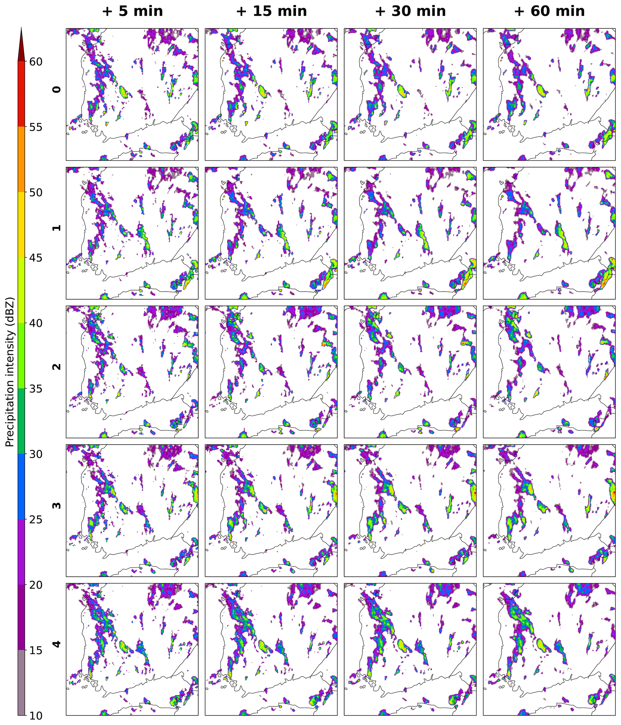
Figure C1Five randomly selected examples of post-processed DEUCE ensemble members on the first case studied, whose area covers southern Finland, starting at 15:00:00 UTC on 9 July 2022. The prediction lead times illustrated are 5, 15, 30, and 60 min.
The data used for the production of the results are available online (Harnist et al., 2023) at https://doi.org/10.23728/fmi-b2share.3efcfc9080fe4871bd756c45373e7c11. These data include the input data used for the training of DEUCE, prediction generation, and observations for the verification. Pre-trained model checkpoints, the script used to gather neural network inputs into an HDF5 file, and computed metric data are also included.
The source code with instructions for the reproduction of results is available online (Harnist, 2023) at https://doi.org/10.5281/zenodo.7961954 and from GitHub at https://github.com/fmidev/deuce-nowcasting (last access: 2 May 2024). This code is used for the training and nowcast generation of DEUCE, the production of baseline nowcasts, the computation of metrics, and the creation of figures presenting these metrics.
BH performed the experiments and analysis, developed the methodology, wrote and maintained software, performed the validation, as well as the visualization work, and wrote the original draft. SP acquired funding and resources and also administrated the project. SP and TM jointly supervised BH in this work. BH, SP, and TM took part in the conceptualization and in the review and editing of the paper.
The contact author has declared that none of the authors has any competing interests.
Publisher's note: Copernicus Publications remains neutral with regard to jurisdictional claims made in the text, published maps, institutional affiliations, or any other geographical representation in this paper. While Copernicus Publications makes every effort to include appropriate place names, the final responsibility lies with the authors.
We gratefully acknowledge the Finnish CSC IT Center For Science, for providing us with the computational resources used for the development of the model, and Venkatachalam Chandrasekaran from Colorado State University, for his advice and critical comments regarding the work.
This research has been supported by the Research Council of Finland (grant no. 341964).
This paper was edited by Shu-Chih Yang and reviewed by Jatan Buch and one anonymous referee.
Abdar, M., Pourpanah, F., Hussain, S., Rezazadegan, D., Liu, L., Ghavamzadeh, M., Fieguth, P., Cao, X., Khosravi, A., Acharya, U. R., Makarenkov, V., and Nahavandi, S.: A review of uncertainty quantification in deep learning: Techniques, applications and challenges, Inform. Fusion, 76, 243–297, https://doi.org/10.1016/j.inffus.2021.05.008, 2021. a
Agrawal, S., Barrington, L., Bromberg, C., Burge, J., Gazen, C., and Hickey, J.: Machine Learning for Precipitation Nowcasting from Radar Images, arXiv [preprint], https://doi.org/10.48550/arXiv.1912.12132, 2019. a
Alexander, C., Dowell, D. C., Hu, M., Olson, J., Smirnova, T., Ladwig, T., Weygandt, S., Kenyon, J. S., James, E., Lin, H., Grell, G., Ge, G., Alcott, T., Benjamin, S., Brown, J. M., Toy, M. D., Ahmadov, R., Back, A., Duda, J. D., Smith, M. B., Hamilton, J. A., Jamison, B. D., Jankov, I., and Turner, D. D.: Rapid Refresh (RAP) and High Resolution Rapid Refresh (HRRR) Model Development, 100th Annual AMS Meeting, Boston Convention and Exhibition Center 415 Summer St. Boston, MA, https://rapidrefresh.noaa.gov/pdf/Alexander_AMS_NWP_2020.pdf (last access: 2 May 2024), 2020. a
Ayzel, G., Scheffer, T., and Heistermann, M.: RainNet v1.0: a convolutional neural network for radar-based precipitation nowcasting, Geosci. Model Dev., 13, 2631–2644, https://doi.org/10.5194/gmd-13-2631-2020, 2020. a, b, c
Bauer, P., Thorpe, A., and Brunet, G.: The quiet revolution of numerical weather prediction, Nature, 525, 47–55, https://doi.org/10.1038/nature14956, 2015. a, b
Blundell, C., Cornebise, J., Kavukcuoglu, K., and Wierstra, D.: Weight Uncertainty in Neural Network, in: Proceedings of the 32nd International Conference on Machine Learning, 1613–1622, PMLR, Lille, France, https://proceedings.mlr.press/v37/blundell15.html (last access: 2 May 2024), 2015. a, b, c, d
Bouguet, J.-Y.: Pyramidal implementation of the affine lucas kanade feature tracker description of the algorithm, Intel corporation, 5, http://robots.stanford.edu/cs223b04/algo_tracking.pdf (last access: 2 May 2024), 2001. a
Bowler, N. E., Pierce, C. E., and Seed, A. W.: STEPS: A probabilistic precipitation forecasting scheme which merges an extrapolation nowcast with downscaled NWP, Q. J. Roy. Meteor. Soc., 132, 2127–2155, https://doi.org/10.1256/qj.04.100, 2006. a, b, c
Caceres, J., Gonzalez, D., Zhou, T., and Droguett, E. L.: A probabilistic Bayesian recurrent neural network for remaining useful life prognostics considering epistemic and aleatory uncertainties, Struct. Contr. Health Monit., 28, e2811, https://doi.org/10.1002/stc.2811, 2021. a
Dechesne, C., Lassalle, P., and Lefèvre, S.: Bayesian U-Net: Estimating Uncertainty in Semantic Segmentation of Earth Observation Images, Remote Sens., 13, 3836, https://doi.org/10.3390/rs13193836, 2021. a
Espeholt, L., Agrawal, S., Sønderby, C., Kumar, M., Heek, J., Bromberg, C., Gazen, C., Carver, R., Andrychowicz, M., Hickey, J., Bell, A., and Kalchbrenner, N.: Deep learning for twelve hour precipitation forecasts, Nat. Commun., 13, 5145, https://doi.org/10.1038/s41467-022-32483-x, 2022. a, b
Farquhar, S., Osborne, M. A., and Gal, Y.: Radial Bayesian Neural Networks: Beyond Discrete Support In Large-Scale Bayesian Deep Learning, in: Proceedings of the Twenty Third International Conference on Artificial Intelligence and Statistics, PMLR, 1352–1362, https://proceedings.mlr.press/v108/farquhar20a.html (last access: 2 May 2024), 2020. a
Gal, Y. and Ghahramani, Z.: Dropout as a Bayesian Approximation: Representing Model Uncertainty in Deep Learning, in: Proceedings of The 33rd International Conference on Machine Learning, PMLR, New York, NY, USA, 1050–1059, https://proceedings.mlr.press/v48/gal16.html (last access: 2 May 2024), 2016. a
Graves, A.: Practical Variational Inference for Neural Networks, in: Advances in Neural Information Processing Systems, vol. 24, Curran Associates, Inc., Granada, Spain, 2348–2356, ISBN 978-1-61839-599-3, https://papers.nips.cc/paper_files/paper/2011/hash/7eb3c8be3d411e8ebfab08eba5f49632-Abstract.html (last access: 2 May 2024), 2011. a
Harnist, B.: Probabilistic Precipitation Nowcasting using Bayesian Convolutional Neural Networks, Master's thesis, Aalto University, School of Science, http://urn.fi/URN:NBN:fi:aalto-202208285227 (last access: 2 May 2024), 2022. a, b, c
Harnist, B.: fmidev/deuce-nowcasting: Initial release of the source code for the manuscript, Zenodo [code], https://doi.org/10.5281/zenodo.7961955, 2023. a
Harnist, B., Pulkkinen, S., and Mäkinen, T.: Data for the manuscript “DEUCE v1.0: A neural network for probabilistic precipitation nowcasting with aleatoric and epistemic uncertainties” by Harnist et al. (2023), Finnish Meteorological Institute [data set], https://doi.org/10.23728/FMI-B2SHARE.3EFCFC9080FE4871BD756C45373E7C11, 2023. a
Hersbach, H.: Decomposition of the Continuous Ranked Probability Score for Ensemble Prediction Systems, Weather Forecast., 15, 559–570, https://doi.org/10.1175/1520-0434(2000)015<0559:DOTCRP>2.0.CO;2, 2000. a
Hershey, J. R. and Olsen, P. A.: Approximating the Kullback Leibler Divergence Between Gaussian Mixture Models, in: 2007 IEEE International Conference on Acoustics, Speech and Signal Processing – ICASSP '07, vol. 4, Honolulu, HI, USA, IV–317–IV–320, https://doi.org/10.1109/ICASSP.2007.366913, 2007. a
Hogan, R. J., Ferro, C. A. T., Jolliffe, I. T., and Stephenson, D. B.: Equitability Revisited: Why the “Equitable Threat Score” Is Not Equitable, Weather Forecast., 25, 710–726, https://doi.org/10.1175/2009WAF2222350.1, 2010. a, b, c
Jospin, L. V., Laga, H., Boussaid, F., Buntine, W., and Bennamoun, M.: Hands-On Bayesian Neural Networks – A Tutorial for Deep Learning Users, IEEE Comput. Intell. Mag., 17, 29–48, https://doi.org/10.1109/MCI.2022.3155327, 2022. a
Kedem, B. and Chiu, L. S.: On the lognormality of rain rate, P. Natl. Acad. Sci. USA, 84, 901–905, https://doi.org/10.1073/pnas.84.4.901, 1987. a
Kendall, A. and Gal, Y.: What uncertainties do we need in Bayesian deep learning for computer vision?, in: Proceedings of the 31st International Conference on Neural Information Processing Systems, NIPS'17, Curran Associates Inc., Red Hook, NY, USA, 5580–5590, ISBN 978-1-5108-6096-4, 2017. a, b, c, d
Kingma, D. P. and Ba, J.: Adam: A Method for Stochastic Optimization, in: Proceedings of the 3rd International Conference on Learning Representations (ICLR), San Diego, CA, USA, https://doi.org/10.48550/arXiv.1412.6980, 2015. a
Kullback, S. and Leibler, R. A.: On Information and Sufficiency, Ann. Math. Stat., 22, 79–86, https://doi.org/10.1214/aoms/1177729694, 1951. a
Laroche, S. and Zawadzki, I.: Retrievals of Horizontal Winds from Single-Doppler Clear-Air Data by Methods of Cross Correlation and Variational Analysis, J. Atmos. Ocean. Tech., 12, 721–738, https://doi.org/10.1175/1520-0426(1995)012<0721:ROHWFS>2.0.CO;2, 1995. a
Leinonen, J., Moisseev, D., Leskinen, M., and Petersen, W. A.: A Climatology of Disdrometer Measurements of Rainfall in Finland over Five Years with Implications for Global Radar Observations, J. Appl. Meteorol. Clim., 51, 392–404, https://doi.org/10.1175/JAMC-D-11-056.1, 2012. a
Liu, G., Reda, F. A., Shih, K. J., Wang, T.-C., Tao, A., and Catanzaro, B.: Image Inpainting for Irregular Holes Using Partial Convolutions, in: Computer Vision – ECCV 2018 Proceedings, Part XI, edited by Ferrari, V., Hebert, M., Sminchisescu, C., and Weiss, Y., Lecture Notes in Computer Science, Springer International Publishing, Munich, Germany, 89–105, ISBN 978-3-030-01252-6, https://doi.org/10.1007/978-3-030-01252-6_6, 2018. a
Lucas, B. D. and Kanade, T.: An Iterative Image Registration Technique with an Application to Stereo Vision, in: IJCAI'81: Proceedings of the 7th international joint conference on Artificial intelligence, vol. 2, University of British Columbia Vancouver, B.C., Canada, p. 674, https://hal.science/hal-03697340 (last access: 2 May 2024), 1981. a
Mason, I.: A model for assessment of weather forecasts, Austr. Meteorol. Mag., 30, 291–303, 1982. a, b
Naeini, M. P., Cooper, G., and Hauskrecht, M.: Obtaining Well Calibrated Probabilities Using Bayesian Binning, in: Proceedings of the Twenty-Ninth AAAI Conference on Artificial Intelligence, vol. 29, https://doi.org/10.1609/aaai.v29i1.9602, 2015. a, b
Pan, X., Lu, Y., Zhao, K., Huang, H., Wang, M., and Chen, H.: Improving Nowcasting of Convective Development by Incorporating Polarimetric Radar Variables Into a Deep-Learning Model, Geophys. Res. Lett., 48, e2021GL095 302, https://doi.org/10.1029/2021GL095302, 2021. a
Prudden, R., Adams, S., Kangin, D., Robinson, N., Ravuri, S., Mohamed, S., and Arribas, A.: A review of radar-based nowcasting of precipitation and applicable machine learning techniques, arXiv [preprint], https://doi.org/10.48550/arXiv.2005.04988, 2020. a
Pulkkinen, S., Nerini, D., Pérez Hortal, A. A., Velasco-Forero, C., Seed, A., Germann, U., and Foresti, L.: Pysteps: an open-source Python library for probabilistic precipitation nowcasting (v1.0), Geosci. Model Dev., 12, 4185–4219, https://doi.org/10.5194/gmd-12-4185-2019, 2019. a, b, c
Pulkkinen, S., Chandrasekar, V., and Niemi, T.: Lagrangian Integro-Difference Equation Model for Precipitation Nowcasting, J. Atmos. Ocean. Tech., 38, 2125–2145, https://doi.org/10.1175/JTECH-D-21-0013.1, 2021. a, b, c
Radhakrishnan, C. and Chandrasekar, V.: CASA Prediction System over Dallas–Fort Worth Urban Network: Blending of Nowcasting and High-Resolution Numerical Weather Prediction Model, J. Atmos. Ocean. Tech., 37, 211–228, https://doi.org/10.1175/JTECH-D-18-0192.1, 2020. a
Ravuri, S., Lenc, K., Willson, M., Kangin, D., Lam, R., Mirowski, P., Fitzsimons, M., Athanassiadou, M., Kashem, S., Madge, S., Prudden, R., Mandhane, A., Clark, A., Brock, A., Simonyan, K., Hadsell, R., Robinson, N., Clancy, E., Arribas, A., and Mohamed, S.: Skilful precipitation nowcasting using deep generative models of radar, Nature, 597, 672–677, https://doi.org/10.1038/s41586-021-03854-z, 2021. a, b, c, d
Ritvanen, J., Harnist, B., Aldana, M., Mäkinen, T., and Pulkkinen, S.: Advection-Free Convolutional Neural Network for Convective Rainfall Nowcasting, IEEE J. Sel. Top. Appl., 1–16, https://doi.org/10.1109/JSTARS.2023.3238016, 2023. a, b
Ruzanski, E. and Chandrasekar, V.: Scale Filtering for Improved Nowcasting Performance in a High-Resolution X-Band Radar Network, IEEE T. Geosci. Remote, 49, 2296–2307, https://doi.org/10.1109/TGRS.2010.2103946, 2011. a, b
Schaefer, J. T.: The Critical Success Index as an Indicator of Warning Skill, Weather Forecast., 5, 570–575, https://doi.org/10.1175/1520-0434(1990)005<0570:TCSIAA>2.0.CO;2, 1990. a
Seed, A. W.: A Dynamic and Spatial Scaling Approach to Advection Forecasting, J. Appl. Meteorol. Clim., 42, 381–388, https://doi.org/10.1175/1520-0450(2003)042<0381:ADASSA>2.0.CO;2, 2003. a
Seed, A. W., Pierce, C. E., and Norman, K.: Formulation and evaluation of a scale decomposition-based stochastic precipitation nowcast scheme, Water Resour. Res., 49, 6624–6641, https://doi.org/10.1002/wrcr.20536, 2013. a, b
Shi, X., Chen, Z., Wang, H., Yeung, D.-Y., Wong, W.-K., and Woo, W.-C.: Convolutional LSTM Network: a machine learning approach for precipitation nowcasting, in: Proceedings of the 28th International Conference on Neural Information Processing Systems – Volume 1, NIPS'15, MIT Press, Cambridge, MA, USA, 802–810, 2015. a
Shi, X., Gao, Z., Lausen, L., Wang, H., Yeung, D.-Y., Wong, W.-K., and Woo, W.-C.: Deep learning for precipitation nowcasting: a benchmark and a new model, in: Proceedings of the 31st International Conference on Neural Information Processing Systems, NIPS'17, Curran Associates Inc., Red Hook, NY, USA, 5622–5632, ISBN 978-1-5108-6096-4, 2017. a
Staniforth, A. and Côté, J.: Semi-Lagrangian Integration Schemes for Atmospheric Models – A Review, Mon. Weather Rev., 119, 2206–2223, https://doi.org/10.1175/1520-0493(1991)119<2206:SLISFA>2.0.CO;2, 1991. a
Sun, J., Xue, M., Wilson, J. W., Zawadzki, I., Ballard, S. P., Onvlee-Hooimeyer, J., Joe, P., Barker, D. M., Li, P.-W., Golding, B., Xu, M., and Pinto, J.: Use of NWP for Nowcasting Convective Precipitation: Recent Progress and Challenges, B. Am. Meteorol. Soc., 95, 409–426, https://doi.org/10.1175/BAMS-D-11-00263.1, 2014. a
Sønderby, C. K., Espeholt, L., Heek, J., Dehghani, M., Oliver, A., Salimans, T., Agrawal, S., Hickey, J., and Kalchbrenner, N.: MetNet: A Neural Weather Model for Precipitation Forecasting, arXiv [preprint], https://doi.org/10.48550/arXiv.2003.12140, 2020. a, b
Trebing, K., Stanczyk, T., and Mehrkanoon, S.: SmaAt-UNet: Precipitation nowcasting using a small attention-UNet architecture, Pattern Recogn. Lett., 145, 178–186, 2021. a
Ulichney, R.: Dithering with blue noise, P. IEEE, 76, 56–79, https://doi.org/10.1109/5.3288, 1988. a, b
Valdenegro-Toro, M. and Mori, D. S.: A Deeper Look into Aleatoric and Epistemic Uncertainty Disentanglement, in: 2022 IEEE/CVF Conference on Computer Vision and Pattern Recognition Workshops (CVPRW), IEEE, New Orleans, LA, USA, ISBN 978-1-66548-739-9, 1508–1516, https://doi.org/10.1109/CVPRW56347.2022.00157, 2022. a
Wen, Y., Vicol, P., Ba, J., Tran, D., and Grosse, R. B.: Flipout: Efficient Pseudo-Independent Weight Perturbations on Mini-Batches, in: 6th International Conference on Learning Representations, ICLR 2018, Vancouver, BC, Canada, 30 April–3 May 2018, Conference Track Proceedings, OpenReview.net, https://openreview.net/forum?id=rJNpifWAb (last access: 2 May 2024), 2018. a
Wilks, D. S.: Statistical Methods in the Atmospheric Sciences, Academic Press, 3rd Edn., ISBN 978-0-12-385022-5, 2011. a, b, c, d, e, f, g, h, i, j, k
Woo, S., Park, J., Lee, J.-Y., and Kweon, I. S.: Cbam: Convolutional block attention module, in: Proceedings of the European conference on computer vision (ECCV), Munich, Germany, 3–19, https://doi.org/10.1007/978-3-030-01234-2_1, 2018. a
Xu, L., Chen, N., Yang, C., Yu, H., and Chen, Z.: Quantifying the uncertainty of precipitation forecasting using probabilistic deep learning, Hydrol. Earth Syst. Sci., 26, 2923–2938, https://doi.org/10.5194/hess-26-2923-2022, 2022. a
- Abstract
- Introduction
- Model description
- Experimental details
- Results
- Discussion
- Conclusions
- Appendix A: Additional technical details
- Appendix B: Results of the second case study
- Appendix C: Additional figures
- Code and data availability
- Author contributions
- Competing interests
- Disclaimer
- Acknowledgements
- Financial support
- Review statement
- References