Impacts of spatial heterogeneity of anthropogenic aerosol emissions in a regionally refined global aerosol–climate model

Emissions of anthropogenic aerosol and their precursors are often prescribed in global aerosol models. Most of these emissions are spatially heterogeneous at model grid scales. When remapped from low-resolution data, the spatial heterogeneity in emissions can be lost, leading to large errors in the simulation. It can also cause the conservation problem if non-conservative remapping is used. The default anthropogenic emission treatment in the Energy Exascale Earth System Model (E3SM) is subject to both problems. In this study, we introduce a revised emission treatment for the E3SM Atmosphere Model (EAM) that ensures conservation of mass fluxes and preserves the original emission heterogeneity at the model-resolved grid scale. We assess the error estimates associated with the default emission treatment and the impact of improved heterogeneity and mass conservation in both globally uniform standard-resolution (∼ 165 km) and regionally refined high-resolution (∼ 42 km) simulations. The default treatment incurs significant errors near the surface, particularly over sharp emission gradient zones. Much larger errors are observed in high-resolution simulations. It substantially underestimates the aerosol burden, surface concentration, and aerosol sources over highly polluted regions, while it overestimates these quantities over less-polluted adjacent areas. Large errors can persist at higher elevation for daily mean estimates, which can affect aerosol extinction profiles and aerosol optical depth (AOD). We find that the revised treatment significantly improves the accuracy of the aerosol emissions from surface and elevated sources near sharp spatial gradient regions, with significant improvement in the spatial heterogeneity and variability of simulated surface concentration in high-resolution simulations. In the next-generation E3SM running at convection-permitting scales where the resolved spatial heterogeneity is significantly increased, the revised emission treatment is expected to better represent the aerosol emissions as well as their lifecycle and impacts on climate.

1 Introduction

The presence of lower tropospheric aerosols has significant impacts on air quality. Additionally, aerosols play a crucial role in the energy balance of the Earth system, as they can scatter or absorb radiation and affect the formation, lifetime, and albedo of clouds. Anthropogenic activities, including air pollution, have contributed to a substantial increase in the tropospheric aerosol burden since the pre-industrial era, further intensifying these effects (Bond et al., 2007). According to the report on the Sixth Intergovernmental Panel on Climate Change (IPCC), the effective radiative forcing of anthropogenic aerosols ranges from −0.63 to −1.37 W m⁻² (Smith et al., 2020). Furthermore, recent urban-scale studies have shown that anthropogenic aerosols may impact regional climate by affecting the urban heat island intensity (Han et al., 2020; Yang et al., 2020; Wu et al., 2017) and altering the precipitating systems over urban areas (Rosenfeld et al., 2008; Van Den Heever and Cotton, 2007). Despite the crucial role of anthropogenic aerosols in affecting regional and global climate, significant uncertainties persist in their numerical simulation. One of the large uncertainties is how anthropogenic aerosol emissions are treated in the model (Textor et al., 2006).

Accurate representation of anthropogenic aerosol emissions and their time evolution are crucial for Earth system models (ESMs) and atmospheric chemistry and transport models (Hoesly et al., 2018). Most of these emission sources are spatially heterogeneous at regional and local scales, and their relatively short lifetime in the atmosphere results in a heterogeneous distribution, both geographically and vertically (Koch et al., 2009). For high-resolution simulations, representing this spatial heterogeneity, particularly near emission hotspots, is important to improve aerosol simulation accuracy (Wang et al., 2018, 2014). Furthermore, retaining this heterogeneity can be important since evaluating the model fidelity in areas such as aerosol formation, transport, cloud interactions, and deposition may depend on the accuracy of the prescribed emissions used to drive the models. Using lower-resolution data may result in a loss of heterogeneity, leading to lower accuracy in the aerosol simulation and model evaluations, particularly near the sharp emission gradient zones. This error may be more significant for high-resolution model simulations, often used in regional and urban-scale studies.

The U.S. Department of Energy (DOE) Energy Exascale Earth System Model (E3SM) is a state-of-the-art ESM that aims to produce actionable and accurate predictions of regional trends relevant to Earth system variability and change (Golaz et al., 2019, 2022). The E3SM Atmosphere Model (EAM, Rasch et al., 2019) has a rather comprehensive representation of physical and chemical aerosol processes, which simulates the lifecycle of aerosols and their interactions with clouds and radiation (Wang et al., 2020). However, for the emission of anthropogenic aerosols and their precursors, the default treatment used in the standard and high-resolution EAM configurations has some limitations. First, the current anthropogenic emission treatment does not conserve mass. EAM uses an unstructured cubed-sphere spectral-element (SE) grid due to its advantages over regular latitude–longitude (RLL) grids, such as offering high-resolution capabilities and improved computational scalability through the regionally refined model (RRM) (Taylor and Fournier, 2010; Dennis et al., 2012). Since the prescribed emissions are on an RLL grid, EAM requires spatial interpolation or remapping. For fluxes (i.e., emission flux), the remapping should be done conservatively (Jones, 1999). However, online conservative remapping of external forcing data (including emissions) is not currently available in E3SM. Therefore, EAM linearly interpolates the data to the model-native SE grid, and conservation is lost during the remapping. Second, with the current emission treatment, it is hard to preserve the spatial heterogeneity as in the original emission data. To avoid large conservation errors over the coarser grids, EAM uses low-resolution (∼ 2°) anthropogenic aerosol emission data for simulations performed at the standard resolution or simulations with RRM, so the linear interpolation will cause large errors (see Sects. 2.2 and 3.1 for details). On the other hand, linearly interpolating high-resolution data to low resolution might cause large conservation errors. Therefore, improving the emission treatment in EAM is essential, especially for future E3SM applications with regional refinement at high resolutions, such as convection-permitting scales.

Similar issues in other atmosphere models with unstructured grids are discussed in recent studies (Pfister et al., 2020; Schwantes et al., 2022), and the model-native emission data have been used for better simulating ozone and evaluating the sensitivity to horizontal resolutions. However, these studies did not investigate/report the model sensitivity to the emission change only (original vs. native-grid emissions) and evaluate the impact on simulated aerosol processes due to improved representation of emission heterogeneity. In this study, we revise the anthropogenic emission treatment in E3SM and directly read and apply the conservatively remapped emissions at the model's native (unstructured) grid. The improved treatment conserves the mass fluxes, and it can also help preserve the emission heterogeneity when a high-resolution model or RRM is used. We assess the impact on the simulated aerosol mass concentrations, optical properties, and anthropogenic aerosol forcing estimate, with a focus on the impacts of improved heterogeneity and mass conservation in high-resolution simulations.

This article is organized as follows. In Sect. 2, we describe the original and revised emission implementations and how the emission data are prepared. We also provide an overview of the model simulations and configurations for this study. In Sect. 3, we estimate the error in model emission input, compare model simulations with different emission treatments, and evaluate them against available observations. Finally, we summarize our findings and provide conclusions in Sect. 4.

2 Methods

In this section, we first briefly describe the model used for this study. We then provide an introduction of the original emission implementation and describe how we improve it. The simulation design and observational data used to evaluate the model are also described in this section.

2.1 Model overview

In this study, we utilize the atmosphere component (EAMv2) of the Energy Exascale Earth System Model version 2 (E3SMv2) (Golaz et al., 2022). E3SMv2 has a comprehensive aerosol model representation (Wang et al., 2020), which is based on the four-mode version of Modal Aerosol Module (MAM4, Liu et al., 2016). It represents major anthropogenic and natural aerosol species with four lognormal size modes, including black carbon (BC), primary organic matter (POM), secondary organic aerosol (SOA), marine organic aerosol (MOA), sulfate (SO₄), mineral dust, and sea salt (Wang et al., 2020). The model accounts for various aerosol processes including aerosol microphysics (condensation, nucleation, coagulation, aging, and aerosol water uptake), emissions, sulfur chemistry, simplified SOA formation, dry removal (dry deposition and sedimentation), and wet removal. The model also considers aerosol effects on radiation and cloud formation (Wang et al., 2020; K. Zhang et al., 2022).

EAMv2 employs a spectral-element dynamical core (Taylor and Fournier, 2010; Dennis et al., 2012) as in EAMv1 (Rasch et al., 2019) but utilizes a “physics grid” (pg2 grid) for unresolved physics parameterization and a separate dynamics grid for resolved processes (Hannah et al., 2021). This allows for an increased computational efficiency by reducing the effective resolution for the physics parameterization computations. The standard configuration of the model uses a low “ne30pg2” resolution (LR), which has a grid spacing of ∼ 110 km (∼ 1°) for dynamics and a grid spacing of ∼ 165 km (∼ 1.5°) for physics. E3SMv2 also supports fully coupled regionally refined mesh (RRM) configurations for high-resolution applications. The regionally refined configurations are computationally inexpensive compared to the uniform high-resolution setup and can be useful in identifying highly heterogeneous fields (Wu et al., 2018; Rahimi et al., 2019). One of the supported stable RRM configurations has a high-resolution mesh centered over North America (NA RRM, Tang et al., 2023). The NA RRM setup has a horizontal resolution of ne120pg2 (∼ 28 km dynamics grid and ∼ 42 km physics grid) over North America and a horizontal resolution of ne30pg2 over rest of the globe (Fig. 1b). The high-resolution refined mesh is located approximately within 10 to 80° N and 170 to 10° W. This region covers a significant number of observation sites (AERONET and IMPROVE) for model evaluation (Fig. 1a). NA RRM has a total of 57 816 computational elements or grid cells as opposed to 21 600 in the standard configuration.

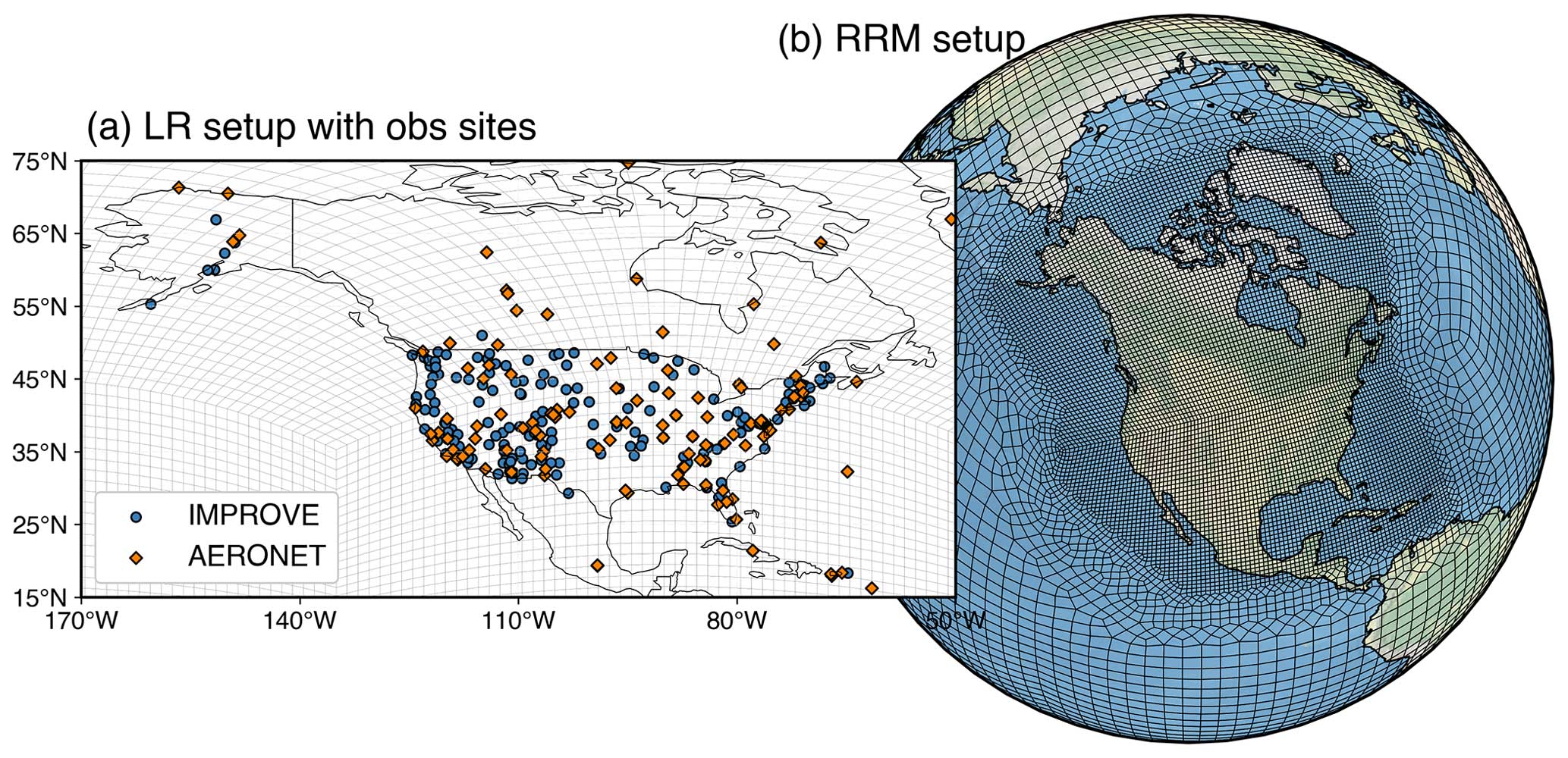
Figure 1 The model-native-grid configuration for the (a) low-resolution, LR (ne30pg2), grid and (b) regionally refined mesh over North America (NA RRM) is shown. The locations for point-source aerosol measurement sites over North America from IMPROVE and AERONET sites are also shown overlaid on the LR grid in panel (a).

In the present study, we conduct experiments in both LR and NA RRM setups to explore the impact of the new emission treatment. More detailed description of the experimental setups is available in Sect. 2.4.

2.2 The original aerosol emission treatment in E3SM

The E3SM accounts for emissions of both natural and anthropogenic aerosols, as well as their precursors (Wang et al., 2020). The emissions of mineral dust, sea salt, and MOA, which are wind-driven primary natural aerosols, are parameterized based on several variables such as surface wind speed, soil erodibility, sea spray fluxes, and sea surface temperature (Zender et al., 2003; Burrows et al., 2022). In contrast, the emissions of BC, POM, SO₄, and precursor gases are prescribed and read in from input data. Note that the emission of dimethyl sulfate (DMS) is also prescribed rather than interactively calculated based on surface wind speed and seawater DMS concentrations in some other global aerosol models (e.g., Zhang et al., 2012). The aerosol particles in these prescribed emission data can be distributed in Aitken mode, accumulation mode, or primary carbon mode (Liu et al., 2012, 2016). All prescribed emissions of BC and POM are considered as primary carbon mode aerosol particles (Liu et al., 2016). EAM assumes 2.5 % of sulfur emissions as primary sulfate aerosol emissions following the AeroCom protocol (Dentener et al., 2006). Sulfate (SO₄) aerosol particles are prescribed as either Aitken or accumulation mode based on the emission sectors or types. Aerosol number emission fluxes are prescribed based on the mass fluxes and the assumed emission particle size distributions (see supplemental materials of Liu et al., 2012). All prescribed aerosol species are emitted as interstitial aerosols at the surface and/or elevated locations.

The anthropogenic emissions from agricultural, industrial, energy, transportation, and domestic sectors for EAMv2 are mostly derived from the Community Emissions Data System (CEDS) inventory (Hoesly et al., 2018). The biomass burning emission is derived from the fourth generation of the Global Fire Emissions Database (GFED4, Giglio et al., 2013; van Marle et al., 2017). CEDS provides historical (1750–2014) inventory of anthropogenic greenhouse gases, reactive gases, and aerosols for the Coupled Model Intercomparison Project Phase 6 (CMIP6, Eyring et al., 2016). It includes anthropogenic emissions for the primary aerosol species, such as BC and OC, and sulfur dioxide (SO₂, a gas precursor for sulfate). These data are in a regular latitude–longitude (RLL) grid at 0.5°×0.5° resolution. GFED4 is also a part of the inputs for CMIP6, which provides a historical (1750–2015) anthropogenic aerosol emission inventory of BC, OC, and SO₂ from biomass burning in an RLL grid at 0.25°×0.25° resolution.

The emission treatment is a key component of the post-coupler processes (see Fig. 2a, excluding the dust emission that is calculated in the land model). It refers to the combination of both the (1) prescribed emission input RLL data (monthly by default) and (2) unified routines to process all prescribed anthropogenic aerosol and precursor gas emissions. For global high-resolution applications (with a uniform grid), EAM can use emission data at higher resolution, where the interpolation error is much smaller. However, for low-resolution (LR) and non-uniform RRM grids, directly using the high-resolution emissions with the default linear interpolation leads to large conservation errors. Figures S1 and S2 illustrate the errors associated with using low- versus high-resolution emissions on coarser grids. When mass flux is not conserved, errors are exacerbated with the incorporation of high-resolution emissions compared to low-resolution emissions. To mitigate these issues in the standard configuration of EAMv2, low-resolution (1.9° × 2.5°) RLL gridded monthly historical (1850–2014) emission data are prescribed for ne30pg2 and RRM simulations. EAM also considers elevated emissions from biomass burning, industrial, energy, and volcanic sources. These emissions are distributed across 13 different altitudes, ranging from the ground level to approximately 7 km above the surface. The distribution of emission within each layer is uniform, but the distribution varies between layers, depending on the source of the emission. Elevated sulfur emissions from energy and industrial sectors are emitted at altitudes between 100 and 300 m above the surface, while biomass burning emissions are distributed across all 13 altitude ranges based on the recommendation from Dentener et al. (2006).

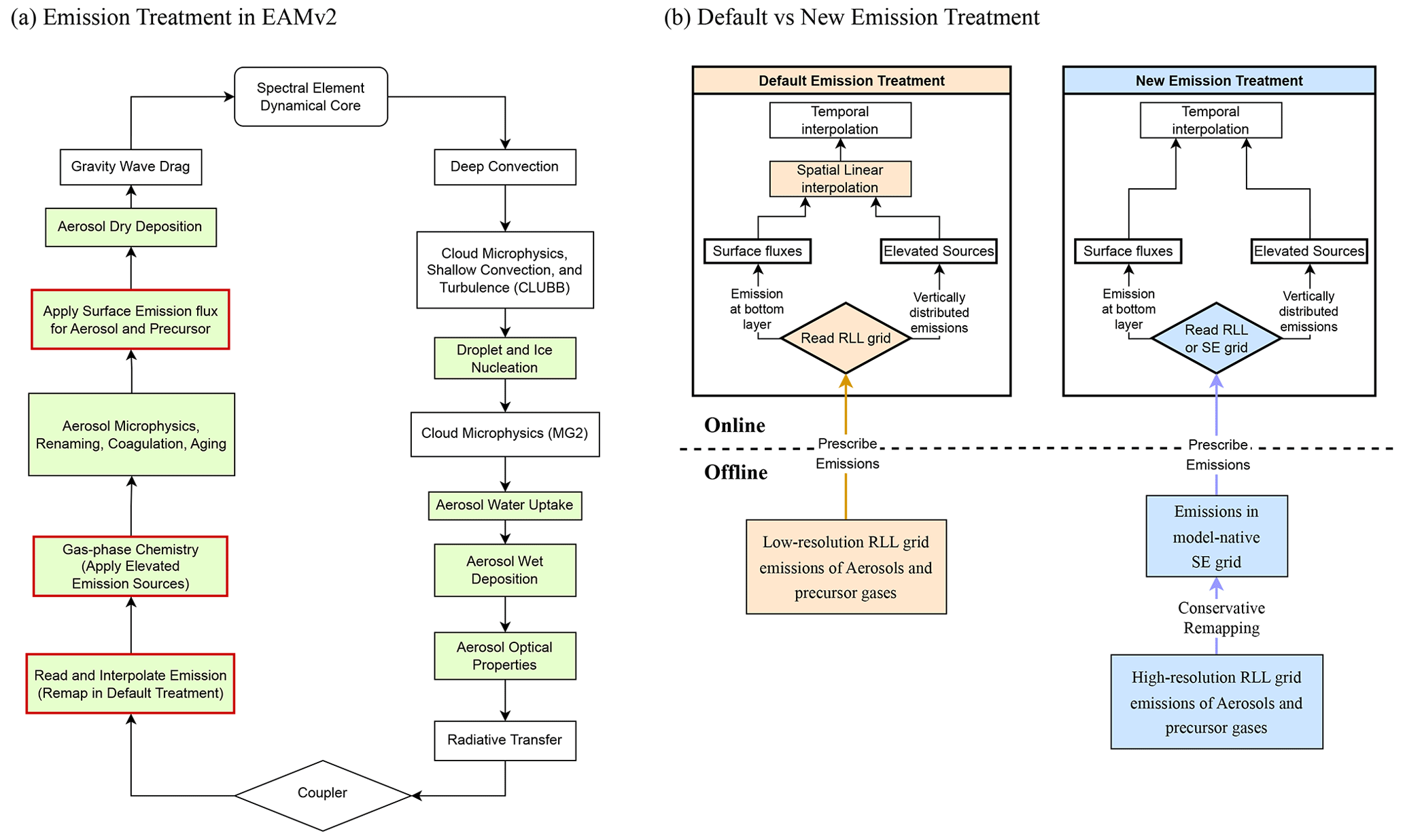
Figure 2 Flowcharts illustrating how the aerosol and precursor gas emission is handled in the EAMv2 simulation. Light green boxes in panel (a) depict the aerosol-related processes, with red bordered boxes indicating emission-related modules impacted during one time step of the physics and dynamics calculations. Panel (b) compares the default and the new emission treatment. The key differences are depicted by light orange and light blue boxes for the default and new emission treatment, respectively.

The default EAMv2 routines read these prescribed emissions in the RLL grid. They are subsequently linearly interpolated to the native model grid, and temporal interpolation is also applied (left panel in Fig. 2b). The aerosol microphysics modules simulate the formation, growth, and removal of aerosols in the atmosphere, including processes of nucleation, coagulation, condensation, and aging. The elevated emissions are applied to the gas-phase chemistry calculations as external forcing terms, while the surface fluxes are updated before dry deposition (Fig. 2a).

As mentioned earlier, linear interpolation is applied to convert the prescribed RLL grid data to the model-native grid in EAMv2 (and earlier versions). Although it is convenient to linearly interpolate the same emission data to the model grid at different spatial resolutions, the current treatment does not conserve mass. Also, when interpolated to higher resolutions, large emission errors will occur compared to the original emission data.

2.3 E3SM revised emission treatment

To address the limitations of the default emission treatment, we revised the emission implementation in EAMv2 as follows (Fig. 2b).

1. We have modified aerosol emission routines, which allows EAM to read prescribed anthropogenic aerosol emissions in both regular latitude–longitude (RLL) and model-native (SE) grids.

2. To preserve spatial heterogeneity and achieve mass conservation, we conservatively remap the RLL high-resolution emission data to the model-native grid at selected resolutions. In addition to remapping, this also involves generating the grids, weights, and mapping files, as well as making the remapped emission data compatible with the revised emission treatment. To simplify and automate this procedure, we developed a Python wrapper package (ggen) that utilizes existing grid-generation and remapping tools (TempestRemap, Ullrich and Taylor, 2015; Ullrich et al., 2016, and ncremap, (Zender, 2008)). This package is applicable to both surface and elevated emissions at any given resolution.

3. The original online linear interpolation is switched off when the new treatment is used to read the conservatively remapped data directly.

The revised treatment has been implemented in both EAMv1 and EAMv2 for scientific evaluations.

In this study, we use the 0.63° × 0.47° RLL grid emission data as the high-resolution emission input for anthropogenic aerosols and precursor gases. The data resolution is close to the ne120pg2 resolution (∼ 42 km for the physics grid), which is the resolution used for refined regions in the NA RRM simulation. These data were prepared for globally uniform high-resolution E3SM applications (Caldwell et al., 2019) using the original CEDS and GFEDv4 data sets as mentioned above. When needed, we can use emission inventories at higher resolutions for simulations at even finer scales.

2.4 Simulations

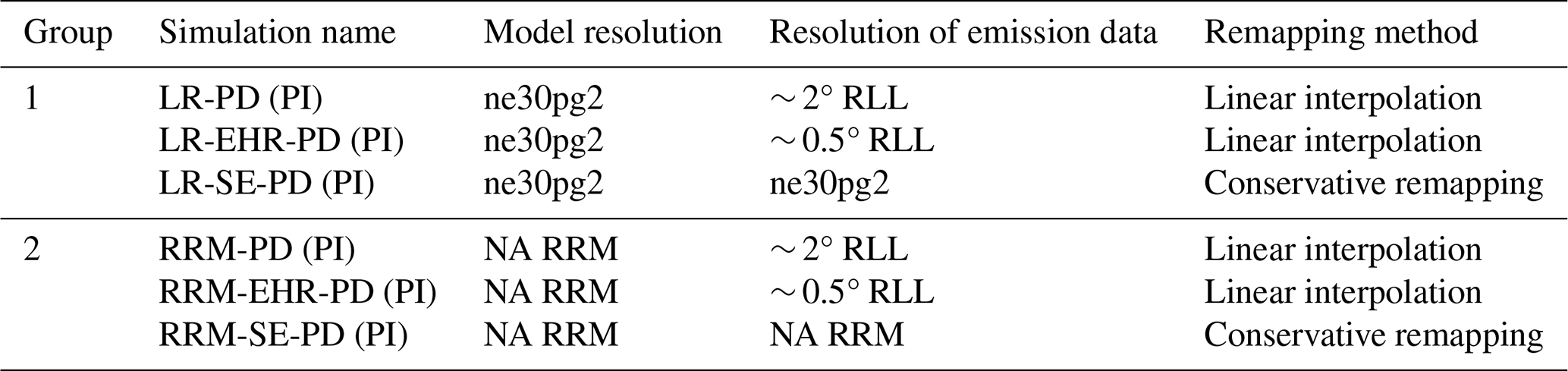
Two groups of E3SMv2 simulations at different horizontal resolutions were conducted to estimate the impacts of the new emission treatment in EAMv2 (Table 1). Each group consists of control simulations using the default emission treatment, simulations using emissions at high resolution (EHR) with default linear remapping, and spectral-element (SE) treatment simulations utilizing the revised emission treatment. The simulations were performed for both the low-resolution standard configuration of E3SMv2 (ne30pg2 or LR) and high-resolution (NA RRM) setup (Fig. 1) with 72 vertical layers. For the control simulations, we follow the standard configuration and use the default low-resolution (1.9×2.5°) prescribed emissions of aerosols and precursor gases in an RLL grid. EHR simulations with high-resolution emissions are similar to control simulations, except the emissions in an RLL grid are at higher resolution (0.63° × 0.47°). For SE simulations, we prepared anthropogenic aerosols and precursor gas emissions on a model-native grid using the same high-resolution data. We conducted simulations with both present-day (PD, year 2014) anthropogenic aerosol emissions and pre-industrial (PI, year 1850) anthropogenic aerosol emissions. All simulations include active atmosphere and land with prescribed monthly mean sea surface temperature and sea ice from 2016. Below we list the objectives of our simulations.

1. We compare LR-PD with LR-SE-PD and RRM-PD with RRM-SE-PD to estimate errors from the default emission treatments. These errors are driven by both heterogeneity and conservation and/or interpolation errors. We identify how aerosol species and processes are disproportionately impacted by these treatments and how they might affect model evaluations when compared to real-world observations.

2. To identify the impact of interpolation error (that leads to conservation error) only, we compare LR-EHR-PD with LR-SE-PD as well as RRM-EHR-PD with RRM-SE-PD.

3. Comparing the error estimates from points no. 1 and 2 above can help us identify the impact of the loss of emission heterogeneity in the standard model.

4. To identify the impact of the loss of emission heterogeneity in the standard model, we compare LR-PD with LR-EHR-PD and RRM-PD with RRM-EHR-PD. All simulations use the original emission treatment, but emissions at different resolutions (latitude–longitude grid) are used for LR and RRM.

5. Present-day (PD) simulations are used for our model assessments. Pre-industrial (PI) simulations are used with PD simulations to calculate aerosol radiative forcings.

Table 1 List of simulations performed and analyzed in this study. All simulations, including three low-resolution (LR, ne30pg2) simulations and three regionally refined model (RRM) simulations, are nudged toward the ERA5 reanalysis. The LR simulations have a dynamics grid spacing of ∼ 110 km (∼ 1°), while the RRM simulations have high-resolution meshes (dynamics grid spacing of ∼ 28 km) over North America but low-resolution meshes (same as LR) for other areas. EHR indicates that high-resolution emission data (∼ 0.5°), instead of the default low-resolution data (∼ 2°), are used as input. RLL refers to the regular latitude–longitude grids. SE refers to the new emission treatment based on model-native spectral-element grids. Present-day (PD) and pre-industrial (PI) simulations are conducted with anthropogenic aerosol emissions from the years 2014 and 1850, respectively.

All simulations were conducted using a meteorological nudging method (Sun et al., 2019), in which the horizontal wind components (u and v) were nudged to the European Centre for Medium-Range Weather Forecasts (ECMWF) ERA5 reanalysis (Hersbach et al., 2020) with a relaxation timescale of 6 h. The nudging data were prepared for both LR and RRM grids, following the method described in S. Zhang et al. (2022), using the 3-hourly ERA5 reanalysis data at 0.25° resolution. Nudging the horizontal winds in these simulations can well constrain the large-scale circulation (Zhang et al., 2014), so that we can (1) assess the impact of model parameterization changes with shorter simulations and (2) carry out a more accurate (co-located) evaluation against in situ measurements than using the free running simulations.

These simulations were performed from 1 October 2015 to 31 December 2016. The first 3 months from the year 2015 were discarded as a model spin-up period, and the remaining 12 months were used for the analysis in this study. The choice of simulation year was based on readily available ERA5 hourly reanalysis data for nudging and active Atmospheric Radiation Measurement (ARM) sites over North America for future evaluations.

2.5 Observation data

To evaluate the model’s ability to simulate regional to local distributions of aerosols with the updated BC, POM, and SO₄ aerosols, aerosol mass concentrations and optical properties (such as aerosol optical depth, AOD) are compared to observational data from regional networks such as the Interagency Monitoring of PROtected Visual Environments (IMPROVE) and Aerosol Robotic NETwork (AERONET) (Fig. 1a). Only present-day (PD) simulations (LR-PD and RRM-PD) were used for the evaluations.

IMPROVE is a network of aerosol monitoring stations located in protected areas in the United States, such as national parks and wilderness areas (Malm et al., 2004). This network measures aerosol properties such as surface concentrations, size distribution, composition, and optical properties. IMPROVE surface concentration measurements are only available over the United States and provide daily data three times a week. For this evaluation, we consider daily average surface concentration measurements from all available IMPROVE sites for each aerosol species in the year 2016. Measurements are available from over 150 sites for BC, organic carbon (OC), and sulfate aerosol surface concentration. We also multiply the observed OC by 1.4 before comparing against simulated POM. Since the IMPROVE measurements are for fine aerosol particles, we do not consider simulated aerosols in coarse mode. We also applied a conversion factor of $\mathrm{96}/\mathrm{115}$ (∼ 0.83) to the simulated sulfate concentration (MAM4 in E3SM assumes the sulfate composition is ammonium bisulfate) before comparing against the IMPROVE measurements.

On the other hand, AERONET, a global network of ground-based sun photometers, measures aerosol properties such as size distribution, composition, and optical properties (Holben et al., 1998). For this evaluation, we used AOD spectral radiometer daily mean measurements from over 120 active sites during the simulation year (e.g., 2016), which fall within the North America high-resolution mesh (bounded by 15 to 75° N and 55 to 170° W) in the RRM setup.

The simulated daily mean data were spatiotemporally co-located with the observational data according to the time and location of each active observational site. These daily average data were conditionally sampled based on EAMv2 emission differences found between the default and revised treatment (see details in Sect. 3.3). We consider the same sites for RRM and LR simulation evaluations. Finally, monthly means of these spatiotemporally collocated data were used to compare simulated and observed surface concentrations and AOD.

3 Results and discussions

3.1 Improving emissions in EAM

One primary goal of our revised emission treatment is to improve the accuracy of the emission data utilized in the standard LR and RRM simulations. The default EAM emission treatment fails to preserve spatial heterogeneity or conserve mass, resulting in substantial errors (as described in Sect. 2.2). Figure 3 shows the spatial distribution of surface BC (a–d) and column-integrated SO₂ emissions (e–h) over the eastern and western US for the year 2014 in the original high-resolution data, the default emission treatment on the RRM grid, the RRM-EHR-PD simulation, and the revised treatment on the RRM grid. The anthropogenic emissions of BC and POM are dominated by surface sources. SO₂ is the primary precursor of sulfate aerosols, and the emission is dominated by the elevated sources over land. Figure 3 indicates how well the heterogeneity of prescribed surface and elevated emissions is represented in the standard RRM simulations when compared against the original high-resolution data.

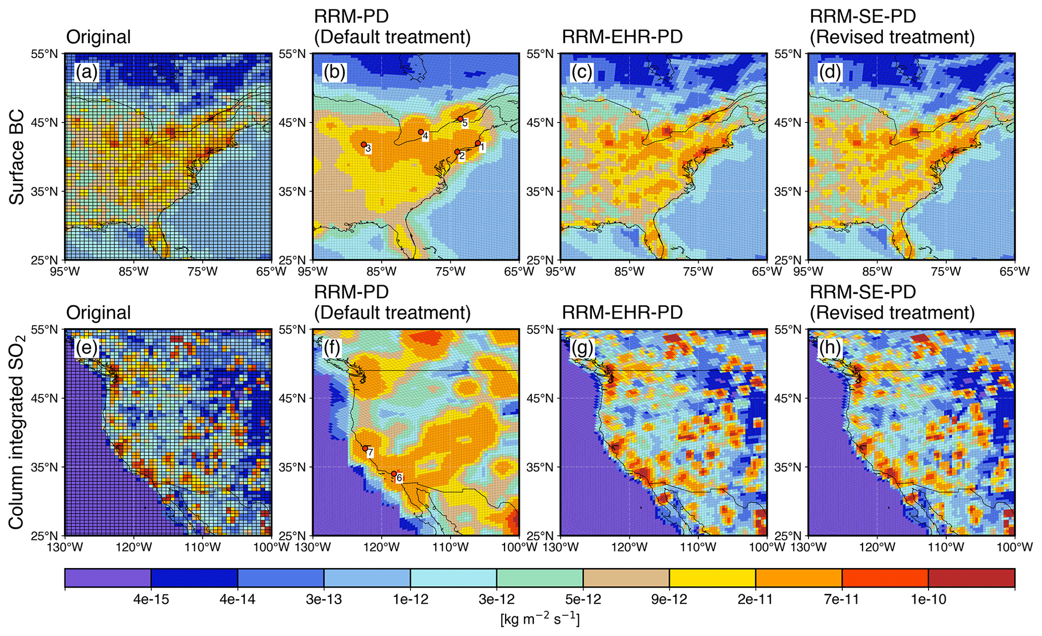
Figure 3 Spatial distribution of the present-day surface BC emissions (top) and column-integrated SO₂ emissions (bottom) from the original high-resolution data (a, e), the RRM-PD (default emission treatment) (b, f), the RRM-EHR-PD (c, g), and the RRM-SE-PD (revised emission treatment) (d, h) simulations. SO₂ emissions are taken from elevated sources (i.e., energy, industrial, biomass burning, and volcanic sources). Distributions are shown over the eastern (top row) and western (bottom row) United States for BC (SO₂) emissions in kg m⁻² s⁻¹ units. Red circles in panels (b) and (f) indicate major cities with large anthropogenic BC and SO₂ emissions, respectively. Markers titled 1, 2, 3, 4, 5, 6, and 7 depict Boston, New York, Chicago, Toronto, Montreal, Los Angeles, and San Francisco, respectively.

The original high-resolution data (Fig. 3a, e) show highly heterogeneous emissions over land, largely driven by industrial, energy, and transportation sectors. As expected, the default emission treatment fails to capture most of the heterogeneity over sharp emission gradient zones (Fig. 3b, f). For example, panels (b) and (f) depict seven major cities (e.g., Boston, New York, Chicago, Toronto, Montreal, Los Angeles, and San Francisco) with large anthropogenic BC and SO₂ emissions, respectively. The default treatment not only significantly underestimates emissions (∼ 80 %) from those cities, but also grossly misrepresents emissions in the nearby regions. This can severely affect the accuracy of high-resolution studies in urban regions. Additionally, the default treatment provides an inaccurate representation of emissions near the coasts, where regions of BC sources from shipping sectors appear to come from comparatively large emissions from transport and industrial sectors over land. In general, both surface and vertically distributed emissions in the default treatment fail to maintain emission land–sea contrast near the coastlines. In contrast, panels (c) and (g) and panels (d) and (h) illustrate the spatial emission distributions in the RRM-EHR-PD simulation and the improved treatment, respectively, which accurately preserves the original spatial heterogeneity both inland and near the coast. Figure 3 illustrates regions on a high-resolution mesh within the North American RRM (NA RRM). In these regions, the predominant cause of inaccuracies is driven by loss of heterogeneity (Table 2). As a result, the data displayed in panels (c) and (g) correspond to similar patterns to those in panels (d) and (h) (revised emission treatment), while RRM-PD shows a large difference in the pattern from the other cases.

Table 2 EAMv2 anthropogenic aerosol emission data statistics in the default emission treatment for present-day (PD) RRM simulations. Statistics are shown for both the surface and elevated emissions of different aerosol species. All estimates are over the North American land (bounded by 15–75° N and 50–170° W). Mean values indicate the area-weighted mean emission fluxes. NMB, NStdDevB, and N_RMSE are defined as $\left(\frac{\sum ({\mathrm{emis}}_{\mathrm{lin}}-{\mathrm{emis}}_{\mathrm{accurate}})}{\sum {\mathrm{emis}}_{\mathrm{accurate}}}\right)\times \mathrm{100}\mathit{\%}$, $\frac{{\mathrm{stdDev}}_{\mathrm{lin}}-{\mathrm{stdDev}}_{\mathrm{accurate}}}{{\mathrm{stdDev}}_{\mathrm{accurate}}}$, and $\frac{\mathrm{RMSE}}{{\mathrm{stdDev}}_{\mathrm{accurate}}}\times \mathrm{100}\mathit{\%}$, respectively. The subscript “accurate” indicates data that preserve spatial heterogeneity and conserve mass. The subscript “lin” indicates linearly interpolated data used in the default treatment. NMB, NStdDevB, RMSE, and N_RMSE before (after) the slash are estimates for RRM-PD (RRM-EHR-PD). Units of mean, StdDev, and RMSE are in kg m⁻² s⁻¹. N_RMSE and NMB are in percentage (%). NStdDevB is unitless.

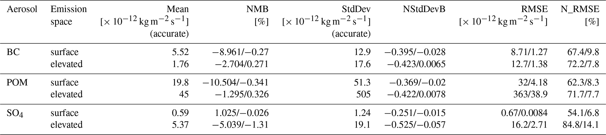
Figure S3 depicts the large error regions in terms of the emission difference between the improved and default treatment from surface and elevated sources. It also indicates that larger errors, from sharper spatial gradients, exist near regions with larger emissions. For instance, the difference between surface BC and POM is much larger over the eastern US, which is consistent with the larger surface emissions over the eastern US. This is important to separate the regions with sharper spatial gradients in the later sections. The improved implementation, which retains both heterogeneity and mass conservation, provides a more accurate representation of surface and vertically distributed emissions in EAMv2. It also accurately applies prescribed emissions in major cities, making the revised treatment suitable for urban-scale studies when running at high resolutions.

To evaluate the loss of accuracy of the EAMv2 emissions in the default treatment, we calculate error estimates against the more accurate emission data from the original high-resolution data (Table 2). Table 2 provides a summary of the error estimates for BC, POM, and SO₄ aerosol emission data used in the EAMv2 RRM simulations, including area-weighted spatial mean (mean), normalized mean bias (NMB), standard deviation (StdDev), normalized standard deviation (NStdDevB), root mean square error (RMSE), and normalized RMSE (N_RMSE) for the present day (year 2014). The estimations for elevated sources are based on column-integrated values. Table S1 in the Supplement presents the error statistics for emissions in the LR simulations. The RRM configuration used in this study has a high-resolution mesh over North America (NA), with the largest sources of emissions occurring over the land and only emissions from the shipping sector occurring over the ocean. Therefore, we consider NA land surfaces bounded by 15 to 75° N and 55 to 170° W for the error estimates.

The default treatment for anthropogenic aerosol emissions in both LR and RRM simulations consistently yields large RMSE for all metrics. It is worth noting that the NMB, which indicates mass conservation errors, is generally small (< 1 %) for the global mean estimate. However, it can be considerably larger for regional estimates, such as BC over the northeast United States, where it can reach up to 25 % (not shown). Over NA land areas, it varies from ∼ 1 % to ∼ 10 % for RRM and ∼ 0.3 % to ∼ 2.5 % for LR emissions. Since NMB is influenced by the magnitude of emissions, it tends to be larger for anthropogenic emission sources than for biomass burning sources. As a result, we observe larger NMB for surface emissions of BC and POM. On the other hand, it is larger for elevated sources of SO₄ aerosol emissions, which includes vertically distributed anthropogenic sources from industry and energy sectors as well as biomass burning sources. This is consistent with larger sulfate aerosol emission differences from elevated sources between the improved and default treatment (Fig. S3). Regardless of the NMB values, we find that both surface and elevated sources exhibit large RMSE values. To compare the RMSE values across different species and sources, we use normalized RMSE (N_RMSE) values. We found consistently larger N_RMSE values (ranging from 54 % to 84 %) for EAMv2 RRM emissions compared to the LR emissions (ranging from 34 % to 57 %), with the largest N_RMSE for the elevated sources of sulfate aerosols.

As expected, the emission errors in RRM-EHR-PD over the high-resolution mesh are small. Conversely, the errors related to LR-EHR-PD emissions can be significant, as indicated in Table S1. On the other hand, in the case of non-uniform grids like those for RRM-EHR-PD emissions, errors tend to increase on coarser grids (Table S2). It is noteworthy that the EHR simulations utilize the same high-resolution emissions as the SE simulations (revised treatment). Consequently, the primary differences in error estimates between these two simulations are attributed to interpolation errors and/or conservation errors. In contrast, the error estimates from the emissions in RRM-PD and LR-PD simulations include both heterogeneity and interpolation and/or conservation errors. Therefore, it is possible to make an intuitive estimation of the heterogeneity errors alone by comparing the discrepancy in error values between the two sets of emissions.

Overall, the default treatment for anthropogenic aerosol emissions leads to large errors in the input emission in both LR and RRM simulations. Improved emission data prepared for our revised emission treatment can resolve these issues by maintaining the spatial heterogeneity (at corresponding resolutions) and mass conservation.

3.2 Model-to-model comparison

In this section, we compare the simulated fields between default PD and SE-PD simulations to evaluate the error estimates from the default emission treatment and the impact of implementing the revised emission treatment. Corresponding figures, when necessary, with the comparison between the EHR-PD and SE-PD simulations, are included in the Supplement. We constrain these comparisons within regional to local scales over North America to encapsulate large differences within the high-resolution RRM mesh.

3.2.1 Simulated climatological means

In Fig. 4, we present the spatial distribution of annual mean surface concentration resulting from RRM-PD simulation using the default emission treatment, along with the relative differences between RRM-SE-PD and RRM-PD. The results show significant differences over North America with a normalized root mean squared error (N_RMSE) of 39 %, 34 %, and 12 % for BC, POM, and sulfate aerosols, respectively. While the absolute relative differences of BC and POM surface concentrations can reach up to 50 % in some regions, sulfate aerosols exhibit weaker relative differences ranging from 2 %–10 %. This can be partially attributed to the fact that prescribed sulfur emissions are mostly emitted from elevated sources, such as industrial and energy sectors, as opposed to BC and POM emissions, which are primarily emitted at the surface level. This difference can also be driven by chemical production and vertical mixing within the boundary layer. Furthermore, significant differences were found in simulated surface concentrations for LR simulations, with normalized RMSE of 19 %, 15 %, and 8 % for BC, POM, and sulfate aerosols, respectively (Fig. S4). The weaker N_RMSE in LR simulations compared to RRM simulations is consistent with the weaker N_RMSE found from the default surface emissions used in the LR experiments (Table S1). Figure S5 illustrates the difference against RRM-EHR-PD, which shows significantly reduced N_RMSE (∼ 5 %) compared to RRM-PD in simulating aerosol surface concentrations over North America. This is expected since most of the errors over high-resolution RRM mesh are driven by the heterogeneity errors in RRM-PD (Table 2).

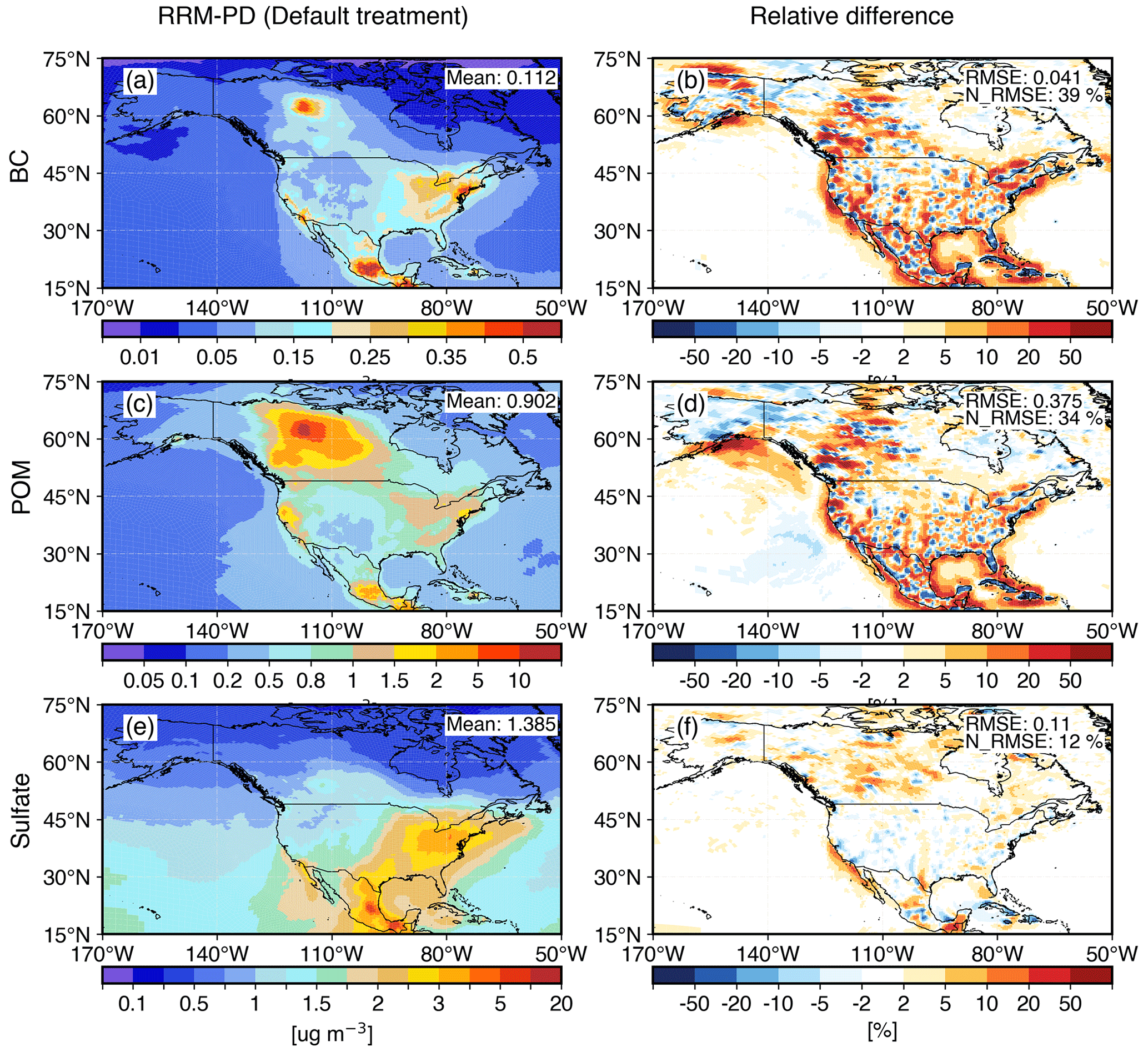
Figure 4 Simulated spatial distribution of annual mean aerosol surface concentration from RRM-PD (a, c, e) and the relative difference between RRM-SE-PD and RRM-PD (b, d, f) over North America. Distributions are shown for (a, b) black carbon (BC), (c, d) primary organic matter (POM), and (e, f) sulfate aerosols. The relative difference for field X is calculated as $\left(\frac{X_{\mathrm{def}}-X_{\mathrm{se}}}{X_{\mathrm{se}}}\right)\times \mathrm{100}\mathit{\%}$, where the “se” and “def” subscripts refer to the simulations with new and default emission treatment, respectively. Mean, RMSE, and normalized RMSE (N_RMSE) are indicated at the top-right corner of the panels. Mean and RMSE has a unit of µg m⁻³. N_RMSE is defined as in Table 2.

Simulated surface concentration differences exhibit positive and negative bias regions, indicating patterns of sharp spatial gradients. Although these patterns appear randomly distributed across North America, they are closely linked to the differences between prescribed emissions from the new and default treatment (Fig. S3). To confirm this, we separated North America into three distinct regions based on the prescribed emission differences between the RRM-SE-PD and RRM-PD simulations. Masking was applied to distinguish regions with strong and weak errors from default emissions. Regions with aerosol emission differences above the 75th percentile, below the 25th percentile, and within the 25th/75th percentiles over North America were selected.

Figure 5 shows the relative differences between different simulated fields, including aerosol burden, surface concentration, net aerosol sources, and sinks. Each field is masked based on their respective aerosol emission difference beyond and within the 25th/75th percentiles. Sharp spatial gradients are predominantly found near highly polluted regions, and fields masked by emission differences above (below) 75th (25th) percentiles reveal larger positive (negative) relative differences. While the estimates vary among different aerosol species and fields, the relative difference can range from −90 % to over 50 %. In contrast, simulated fields masked by emissions within 25th/75th percentiles, representing weaker emission gradients, show significantly smaller relative differences, ranging from 0.3 % to ∼ 5 %. These results suggest that the seemingly random distribution of relative differences in Fig. 4 is strongly linked to the emission differences between the new and default treatment. It also indicates that errors in default emissions not only impact simulated surface concentrations but also aerosol burden (weak) and their sources–sinks (strong). A decomposed source–sink analysis is described in a later section.

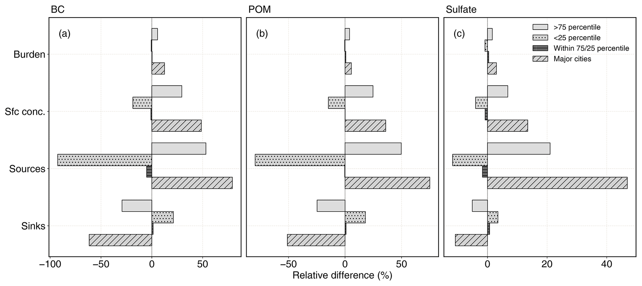
Figure 5 Quantitative distribution of annual mean relative differences between RRM-SE-PD and RRM-PD for simulated aerosol burden, surface concentration, aerosol sources, and aerosol sinks. Distributions are shown for (a) BC, (b) POM, and (c) sulfate aerosols in percentage. Simulated fields are masked by emission differences between the new and default treatment. Masking is applied for regions above the 75th percentile (> 75th percentile), below the 25th percentile (< 25th percentile), and within 25–75th percentiles over North America. Urban-scale differences are also shown considering major cities with larger anthropogenic aerosol emissions.

Figure 5 also displays relative differences from major cities over North America with large anthropogenic aerosol emissions (as depicted in Fig. 3). These cities are located above the 75th percentile masked regions and display similar patterns, with significant positive or negative biases in the simulated aerosol burden, surface concentration, and aerosol sources and sinks. This finding suggests that errors arising from default emissions can have a significant impact on the accuracy of high-resolution urban-scale simulations. We note that the simulated aerosol burden yields weaker relative differences compared to surface concentration. This is expected since we are analyzing long-term annual means of column-integrated concentration (burden), which are influenced by several other processes, such as condensation aging, coagulation, aqueous-phase cloud chemistry, depositions, vertical diffusion, and horizontal transport.

Figure 6 illustrates the spatial distribution of simulated annual mean aerosol extinction and absorption at the model surface layer, as well as AOD and absorption AOD (AAOD). Actual distributions are from RRM-PD simulation, and the differences are between RRM-PD and RRM-SE-PD. From long-term means, we found larger differences in simulated surface aerosol concentration. Therefore, larger relative differences in annual mean aerosol extinction and absorption are constrained near the surface level with a normalized RMSE of 13 % and 29 %, respectively. Our revised treatment improves the anthropogenic aerosol emissions, leading to larger differences in simulated absorption profiles near the surface compared to extinction profiles. Extinction profiles are influenced by natural aerosols such as sea salt and dust, in addition to the anthropogenic aerosols. Notably, aerosol absorption profiles near the surface can reach a relative difference of approximately 50 % over major cities, southern Mexico, and northwestern North America, which is consistent with the spatial distribution of emission differences between the new and default treatment.

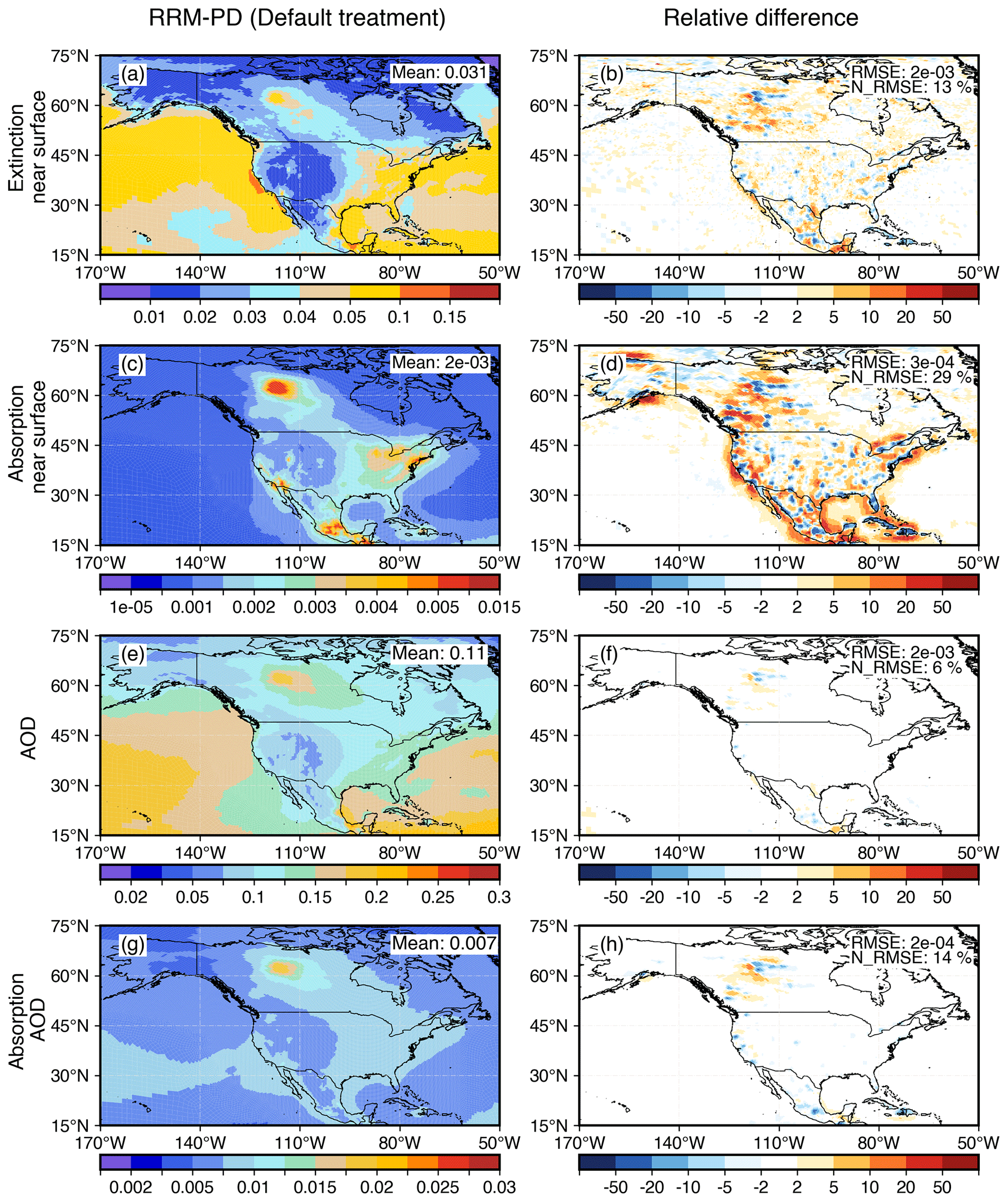
Figure 6 Spatial distribution of annual mean simulated (a, b) aerosol extinction at the surface, (c, d) aerosol absorption at the surface, (e, f) aerosol optical depth (AOD), and (g, h) absorbing AOD from RRM-PD (left column) and the relative difference between RRM-SE-PD and RRM-PD (right column) over North America. The relative difference for field X is calculated as $\left(\frac{X_{\mathrm{def}}-X_{\mathrm{se}}}{X_{\mathrm{se}}}\right)\times \mathrm{100}\mathit{\%}$, where the “se” and “def” subscripts refer to the simulations with new and default emission treatment, respectively. Mean, RMSE, and normalized RMSE (N_RMSE) are indicated at the top-right corner of the panels. Mean and RMSE has a unit of µg m⁻³. N_RMSE is defined as in Table 2.

AOD and absorption AOD are column-integrated aerosol extinction and absorption, respectively, that are strongly influenced by processes such as aerosol chemistry, horizontal transport, and vertical diffusion. Our results indicate that the annual mean spatial distributions of these simulated fields do not show significant differences, with some exceptions over northwestern North America, which can be attributed to the unusually high biomass burning emissions of BC and POM during the 2014 Northwest Territories (NWT) fires. The summer of 2014 was the most severe fire season in NWT history, resulting in wildfires burning a record 3.4×10⁶ ha and an estimated emission of 164 ± 32 Tg of carbon into the atmosphere (Veraverbeke et al., 2017; Kochtubajda et al., 2019). Biomass burning emissions are prescribed as elevated sources of anthropogenic aerosols in E3SM. Substantial errors from default emissions persist at higher elevations (Table 2). Since the present-day simulations are conducted using the emissions from the year 2014, the simulated AAOD shows large relative differences over NWT, which may be driven by the persisting errors in elevated BC and POM emissions from default treatment.

The revised emission treatment has no conservation error. Since there is little to no heterogeneity difference between RRM-EHR-PD and RRM-SE-PD, we can compare them to estimate the impact of conservation errors. We found significantly reduced N_RMSE (∼ 10 %) in near-surface extinction, absorption, AOD, and AAOD (Fig. S6). This is supported by the long-term mean differences in simulated surface aerosol concentrations over North America, depicted in Fig. S5. However, we expect larger impacts over coarser grids, as indicated in Table S3. For instance, Fig. S1c and d and Fig. S2c and d demonstrate the mass conservation errors in BC and SO₂ emissions over coarser grids. These errors in the prescribed emissions may propagate in model simulations and impact simulated aerosol concentrations. Figures 7 and 8 show the simulated BC and sulfate burden differences between RRM-PD, RRM-EHR-PD, and RRM-SE-PD. We note that these column-integrated burdens are also strongly affected by horizontal transport, vertical diffusion, and aerosol chemistry, in addition to emissions. In the refined region (NA), the overall differences between the simulations are small, while in other regions (e.g., East Asia), the differences are much larger, where employing the default treatment (RRM-PD, with low-resolution emission) results in smaller burden differences from RRM-SE-PD (Figs. 7b and 8b) compared to those from RRM-EHR-PD, which uses the high-resolution emission (Figs. 7d and 8d).

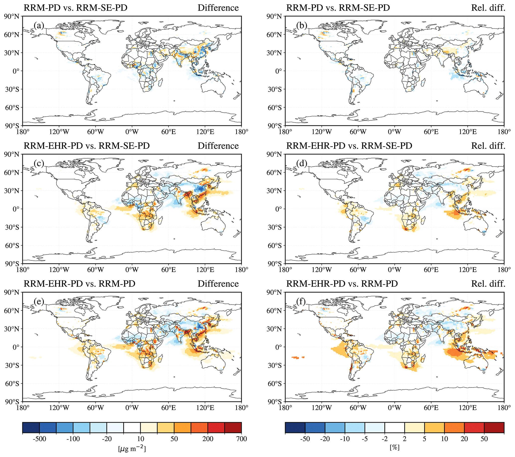
Figure 7 Global distribution of simulated BC aerosol burden differences between (a, b) RRM-PD and RRM-SE-PD, (c, d) RRM-EHR-PD and RRM-SE-PD, and (e, f) RRM-EHR-PD and RRM-PD simulations. All column-integrated burden absolute differences are shown in µg m⁻², and the relative differences are shown in percent (%).

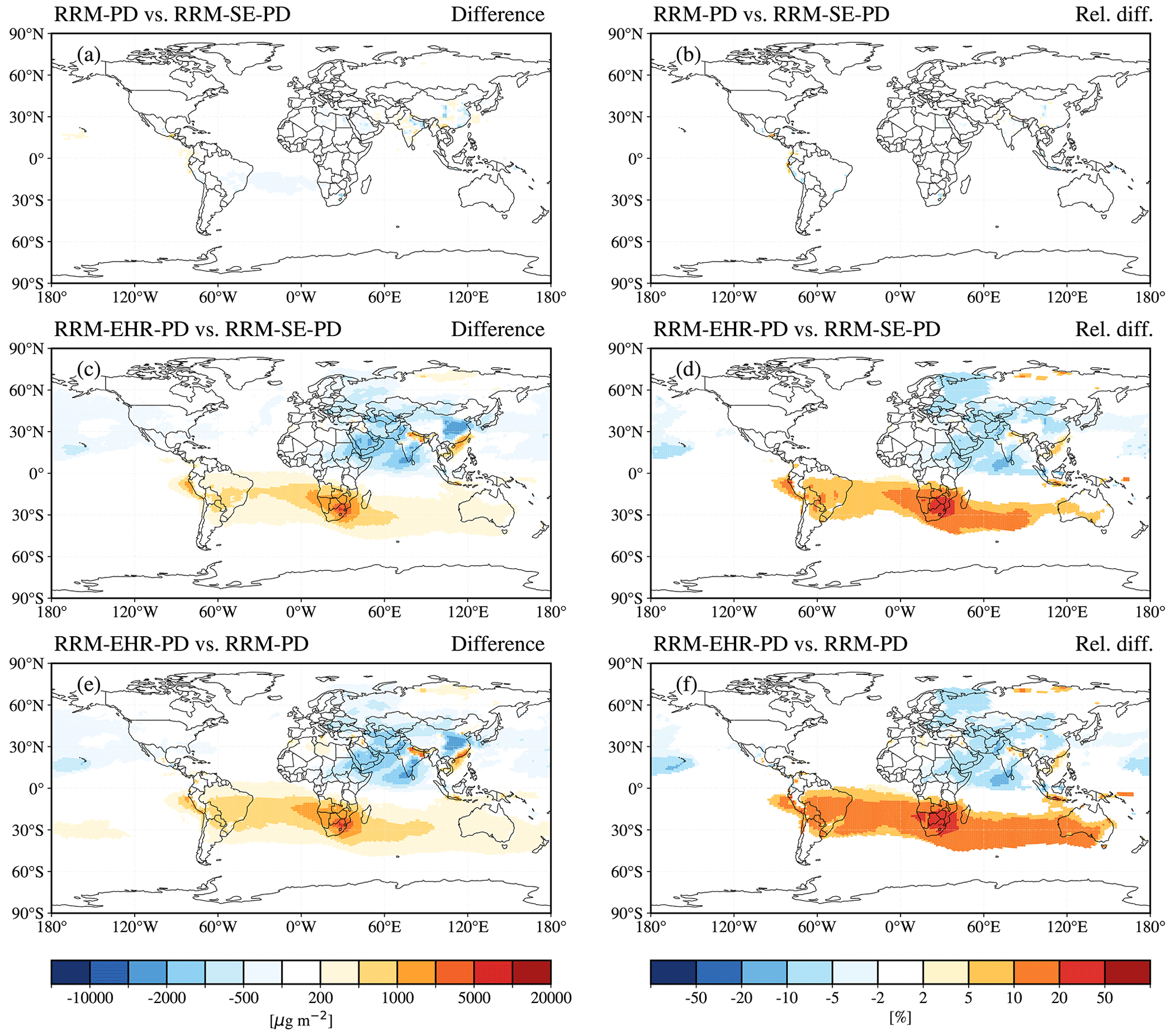
Figure 8 Global distribution of simulated sulfate aerosol burden differences between (a, b) RRM-PD and RRM-SE-PD, (c, d) RRM-EHR-PD and RRM-SE-PD, and (e, f) RRM-EHR-PD and RRM-PD simulations. All column-integrated burden absolute differences are shown in µg m⁻², and the relative differences are shown in percent (%).

3.2.2 Simulated high-frequency fields

While the column-integrated concentration (i.e., aerosol burden) may be less affected, larger discrepancies can arise at the surface level and at higher elevations in high-frequency concentration profiles from RRM-PD (using default treatment). Figure 9 exhibits significant differences in simulated daily mean BC concentration profiles and column-integrated burden. Panels (a)–(d) and (e)–(h) illustrate vertically distributed aerosol concentrations and column-integrated burden from highly (nearby less) polluted locations to demonstrate the simulated biases near sharp spatial emission gradient zones. The vertical profiles indicate that the larger differences can persist at higher elevations above the surface. Over polluted regions, the default emission treatment significantly underestimates surface and elevated aerosol concentration within the boundary layer. On the other hand, over comparatively cleaner nearby regions, the default emission treatment significantly overestimates surface and elevated aerosol concentrations within the boundary layer. Due to the high variance in daily mean fields, as opposed to long-term monthly or annual means, we found significantly larger errors in simulated high-frequency data. For instance, relative differences in simulated BC burden could reach up to ∼ 20 % on certain days (Fig. 9d). Similarly, we found large discrepancies in aerosol concentration profiles from RRM-EHR-PD simulation due to conservation errors (Fig. S7).

High-frequency daily mean AOD and absorption AOD can have N_RMSE values of approximately 15 %–20 % over North America. Figure 10 shows the time series of high-frequency daily mean extinction and absorption profiles, as well as the time evolution of AOD and AAOD during the month of July 2016. The distributions are shown over a highly polluted location as in Fig. 9a–d. We note that the time evolution of the simulated high-frequency absorption profile closely resembles the changes in BC profiles, since the aerosol absorption is primarily influenced by BC. Consistent with the persistent aerosol concentration differences found at higher elevations (Fig. 9), significant differences exist in the simulated extinction and absorption profiles within the boundary layer. Although the long-term annual mean AOD and AAOD do not display significant errors over the highly polluted northeastern US region, relative differences from daily mean estimates could reach up to approximately 10 %–12 % on certain days (Fig. 10d, h). Our results highlight the potential impact of errors from default emission treatment on high-frequency aerosol concentrations at higher elevations, which can further influence aerosol extinction profiles and lead to significant errors in simulated AOD. This finding is particularly relevant as short-term high-frequency fields are often used for urban-scale studies and model evaluations against observations.

3.2.3 Decomposed source–sink analysis

Results in Sect. 3.2.1 suggest that using the default emission treatment can lead to significant errors in aerosol source and sinks, despite having a weaker impact on column-integrated aerosol burden (Fig. 5). In this section, we conduct an aerosol source–sink analysis to estimate the potential errors propagated from default emissions into different processes during the RRM simulations. Figure 11 presents stacked bar plots indicating the fractional distribution of major processes contributing to the total simulated aerosol sources and sinks in the EAMv2 present-day RRM simulation. The analysis considers the North American region (15 to 75° N and 55 to 170° W) and estimates the percent contributions from annual means of each component that drives the simulated sources and sinks. The overall fractional distribution is very similar in LR simulations (not shown).

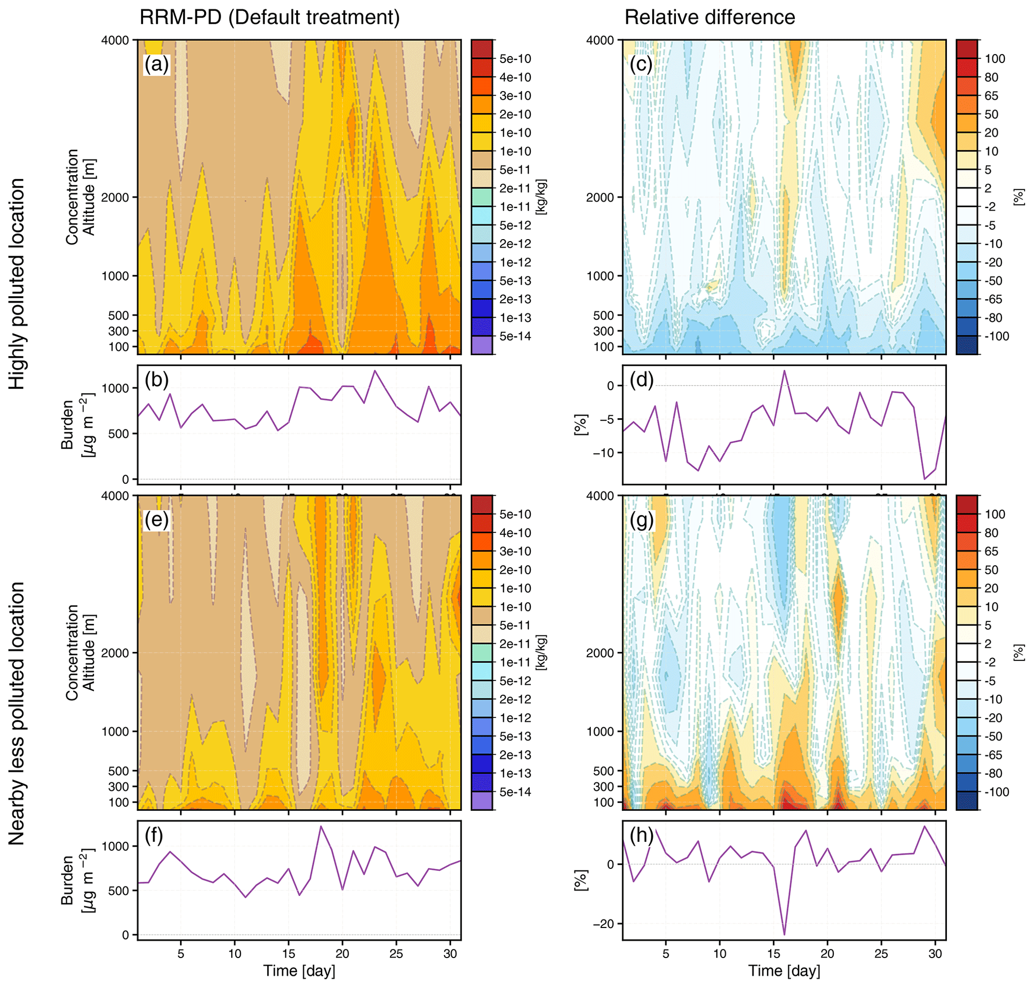
Figure 9 Daily mean black carbon (BC) concentration profile and burden time series during the month of July of 2016 near the sharp spatial emission gradient in eastern North America. Simulated vertical distribution and burden time series from RRM-PD (left column) and the relative difference between RRM-PD and RRM-SE-PD (right column) are shown. Panels (a)–(d) depicts the highly polluted location, with panels (e)–(h) depicting the nearby less-polluted location.

The stacked bar plots in Fig. 11a reveal that prescribed emissions are the primary drivers of BC and POM sources, with a surface (from anthropogenic sources) to elevated (from biomass burning sources) emission ratio of 7:3 for BC and 6:19 for POM, respectively. In contrast, only about 5 % of the total sulfate sources are driven by the prescribed sulfate aerosol emissions. Gas-phase production from SO₂ oxidation and in-cloud aqueous-phase (SO₄) chemistry contribute to sulfate sources by ∼ 22 % and ∼ 71 %, respectively. BC and POM sinks are evenly modulated by dry and wet depositions, with turbulent dry deposition accounting for most of the dry deposition (∼ 41 % and ∼ 36 %) and in-cloud scavenging accounting for most of the wet deposition (∼ 56 % and ∼ 60 %). Stratiform clouds modulate the larger portion of the in-cloud wet deposition. Conversely, sulfate removal has an uneven ∼ 15 % and ∼ 85 % contributions from dry and wet depositions, respectively, with the largest contribution from stratiform in-cloud scavenging (∼ 65 %).

Figures 12 and 13 present the error statistics (in terms of weighted N_RMSE) for the simulated source and sink terms in RRM-PD, taking RRM-SE-PD as the reference solution. The weights are determined by the fractional contributions of each process shown in Fig. 11, and the actual RMSE and N_RMSE for each process can be found in Table S3. The results indicate substantial errors in the RRM-PD simulated aerosol sources, sinks, and their components, which are consistent with the spatial distribution of relative differences shown in Figs. S8–S14.

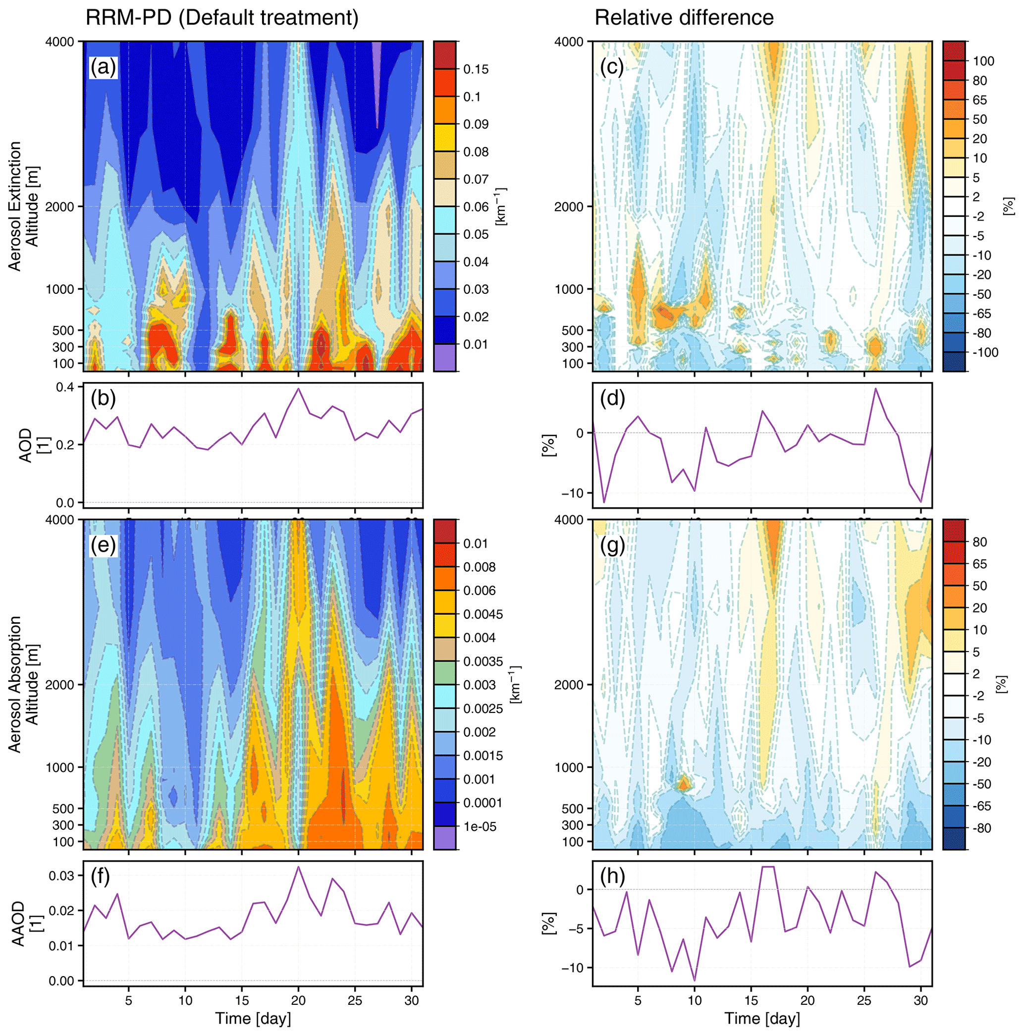
Figure 10 Daily mean aerosol extinction and absorption time series during the month of July of 2016 over the highly polluted location as in Fig. 7 near the sharp spatial emission gradient in eastern North America. Simulated aerosol extinction profile, absorption profile, AOD, and absorption AOD (AAOD) time series from RRM-PD (left column) and the relative difference between RRM-PD and RRM-SE-PD (right column) are shown.

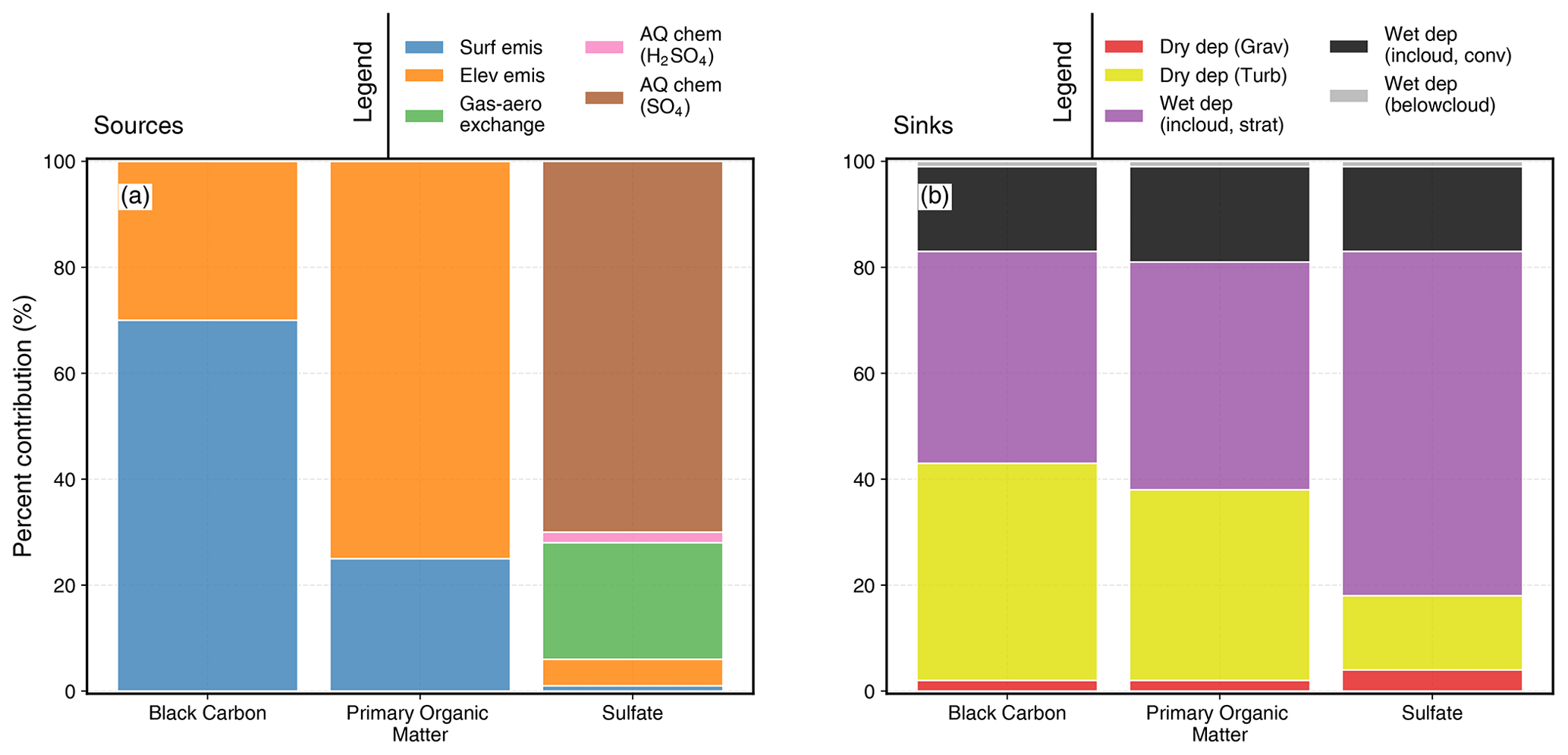
Figure 11 Contribution of the decomposed aerosol source and sink processes in EAMv2 simulations for black carbon (BC), primary organic matter (POM), and sulfate (SO₄) aerosols. All estimates are from annual means over North America. Legends for sources and sinks are shown separately at the top-right corner of each panel. Decomposed dry deposition processes “Grav” and “Turb” refer to the gravitational settling and turbulent deposition, respectively. “AQ chem (SO4)” refers to aqueous-phase chemical production through oxidation of SO₂ by hydrogen peroxide and ozone. “AQ chem (H2SO4)” refers to aqueous-phase chemical production through cloud-water uptake of H₂SO₄. In-cloud wet deposition refers to the nucleation scavenging, and below-cloud wet deposition is the washout (or impaction scavenging) by rain or snow.

The N_RMSE for both BC and POM total sources is approximately 71 %. However, the error contributions from anthropogenic sources are much larger for BC, with a contribution of about 49 %, compared to POM, which has a contribution of about 16 %. POM errors are primarily driven by the biomass burning sources. This difference is due to the spatial variability and magnitudes of biomass burning emissions (BB) in 2014, which are reflected in the surface and elevated emission ratios of BC and POM. It should be noted that the contribution from BB sources (e.g., elevated emission) is comparatively significant over NA due to the 2014 Northwest Territories fires. For BC, larger BB sources are concentrated within northwestern NA, while anthropogenic sources are prevalent over the rest of NA (Fig. S8). In contrast, for POM, the BB sources have a significantly larger contribution and the large anthropogenic sources are concentrated over eastern and southern NA (Fig. S10). These source contributions are reflected in the spatial distribution and magnitude of relative differences, resulting in an uneven error contribution to BC and POM from different emission sources.

Total simulated aerosol sink yields a N_RMSE of ∼ 34 % from BC and POM, respectively, with the largest contributions from dry deposition (Fig. 12). This is consistent with the spatial distribution of relative differences over NA between RRM-SE-PD and RRM-PD in Figs. S9 and S11. Aerosol dry deposition in EAMv2 depends on gravitational settling and turbulent deposition velocities, and at the surface turbulent deposition is substantially larger for BC and POM. Our results show that over 99 % of the N_RMSE in dry deposition comes from turbulent dry deposition flux, which is consistent with the fractional distribution of sinks in Fig. 11.

N_RMSE for wet deposition components for POM and BC are significantly smaller than dry deposition, which is inconsistent with the fractional contribution of sinks. EAMv2 aerosol wet deposition treatment considers both in-cloud and below-cloud scavenging by stratiform and convective precipitation (Barth et al., 2000; Rasch et al., 2000). In-cloud scavenging is the dominant driver of total wet deposition, so we focus on the stratiform and convective in-cloud scavenging analysis in EAMv2. In-cloud scavenging through stratiform clouds considers only the cloud-borne aerosol particles, while in convective clouds both the cloud-borne and interstitial aerosols are affected. For convective in-cloud scavenging, EAM uses a unified convective transport and removal treatment, which considers secondary activation for aerosols into convective updrafts and a subsequent in-cloud wet removal (Wang et al., 2020, 2013). BC and POM in the primary carbon mode are not directly affected by the convective in-cloud scavenging. However, they can be converted to the accumulation mode particles through condensation aging and coagulation, which are strongly affected by the convective removal. Similarly, stratiform in-cloud scavenging strongly affects stratiform cloud-borne BC and POM in the accumulation and coarse modes, which are formed via droplet nucleation. Since neither of the in-cloud scavenging routines directly affects the prescribed BC and POM in primary carbon mode, we observe a weaker error contribution from wet deposition, despite its strong contribution to the total aerosol sinks.

For sulfate aerosols, the simulated source and sink yield a N_RMSE of ∼ 36 % and ∼ 9 %, respectively (Fig. 13). The error estimates for sources align with the fractional distribution of each component, with the largest contributions from gas–aerosol exchange and in-cloud aqueous-phase (SO₄) chemistry. Sulfate sinks yield significantly smaller errors compared to BC and POM, consistent with the weaker contribution from dry deposition. Interestingly, we see larger error contributions from wet deposition, with stratiform in-cloud scavenging accounting for more than half of it. Prescribed sulfate aerosol emissions are in the Aitken and accumulation modes, which are hygroscopic and can be directly affected by convective in-cloud scavenging. On the other hand, the sulfate production through in-cloud aqueous-phase chemistry is attributed to cloud-borne aerosol particles in stratiform clouds. These particles are subsequently removed through stratiform in-cloud scavenging, which is the largest contributor to total wet deposition. The error estimates for each sink component are consistent with their fractional contributions to the total simulated sulfate sink. Therefore, we see larger N_RMSE from in-cloud wet depositions for sulfate aerosols.

Overall, our analysis highlights significant errors in simulated aerosol sources and sinks when the default emission treatment is used. Larger simulation errors are evident for BC and POM source–sink components, primarily due to the prescribed emissions and dry depositions.

3.3 Model evaluation against observations

To demonstrate the improved heterogeneity resulting from the revised emission treatment, ideally it would be nice to evaluate the model against observations near locations with a sharp emission gradient, where the linear interpolation of coarse-resolution data causes large errors. The sharpest gradients in BC emissions are found over the northeastern US (see emission difference shown in Fig. S3a), while for the central and western US, the emission spatial gradient is weaker. Consequently, many observational network sites (e.g., IMPROVE and AERONET, which mainly represent regional background conditions) do not fall within or near the regions with large errors.

To address this issue, we have applied conditional sampling based on the emission differences between the new and default treatment. Specifically, we select sites where the emission differences are above (below) the 75th (25th) percentiles. Using the 90th/10th percentiles yields similar results, but with a reduced number of sites. Without conditional sampling, sites falling within the 75th/25th percentiles can mask the impact of the revised treatment (not shown). Conditional sampling raises the likelihood of selecting sites over large error regions, assuming larger gradients occur near larger biases.

In Fig. 14, we evaluate the simulated BC and POM surface concentrations in RRM-PD, RRM-EHR-PD, and RRM-SE-PD against observations from IMPROVE (described in Sect. 2.5). A similar evaluation for LR simulations is shown in Fig. S15. Figure 14 shows substantial improvements in simulated surface concentrations of BC and POM with RRM-SE-PD. The spatial correlations between the simulated and observed surface concentrations are increased from 0.44 to 0.59 for BC and 0.45 to 0.52 for POM, when the revised emission treatment (RRM-SE-PD) is applied. Our results suggest significant improvements in spatial heterogeneity in terms of the spatial correlation coefficient for BC (with Fisher's Z of −1.8 at p≤0.05) and potential improvements for POM (with Fisher's Z of −1.2 at p≤0.1). Since the primary source of errors over the refined region is driven by the loss of heterogeneity, RRM-EHR-PD shows similar improvements over RRM-PD.

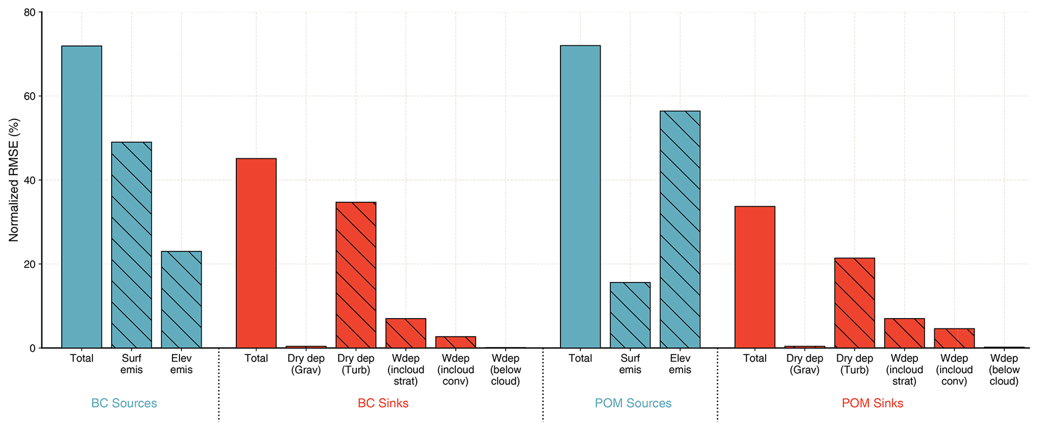
Figure 12 Error estimates of the total and decomposed processes contributing to the simulated sources and sinks of BC and POM from present-day (PD) RRM simulations. All RMSE estimates are over the North America land surface. Normalized RMSE is defined as $\mathrm{N}\mathit{\_}{\mathrm{RMSE}}_{\mathrm{Total}}\times \frac{{\mathrm{Weight}}_i\times \mathrm{N}\mathit{\_}{\mathrm{RMSE}}_i}{\sum ({\mathrm{Weight}}_i\times \mathrm{N}\mathit{\_}{\mathrm{RMSE}}_i)}$, where N_RMSE is defined as in Table 2, weights are from Fig. 6, and subscript “i” indicates decomposed process. The solid bars represent the normalized RMSE for the total source and sink. The hatched bars are the decomposed processes normalized to the total N_RMSE values. The “Wdep” bars refer to the wet deposition components.

Figure 13 Error estimates of the total and decomposed processes contributing to the simulated sources and sinks of sulfate aerosols from present-day (PD) RRM simulations. All RMSE estimates are over the North America land surface. Normalized RMSE is defined as $\mathrm{N}\mathrm{\_}{\mathrm{RMSE}}_{\mathrm{Total}}\times \frac{{\mathrm{Weight}}_i\times \mathrm{N}\mathrm{\_}{\mathrm{RMSE}}_i}{\sum ({\mathrm{Weight}}_i\times \mathrm{N}\mathrm{\_}{\mathrm{RMSE}}_i)}$ , where N_RMSE is defined as in Table 2, weights are from Fig. 6, and subscript “i” indicates decomposed process. The solid bars represent the normalized RMSE for the total source and sink. The hatched bars are the decomposed processes normalized to the total N_RMSE values. The “Wdep” bars refer to the wet deposition components.

In Fig. 15, we present the distribution of daily mean surface concentrations of BC and POM using the conditionally sampled sites (as in Fig. 14). It shows that RRM-PD consistently underestimates the seasonal means and the variability of observed daily mean measurements. This underestimated variance can be attributed to an inaccurate representation of spatial heterogeneity in the default emission treatment. Both RRM-SE-PD and RRM-EHR-PD reduce the seasonal mean biases along with improved variability in simulated daily mean surface concentration. We note that using emissions from the year 2016 (which are unavailable for EAMv2) in the simulations will provide more accurate comparisons (as discussed in Sect. 2.4). However, the overall changes in global emissions are small (∼ 10 %) and are unlikely to significantly affect the simulated surface concentrations. For example, the total anthropogenic BC emissions over North America decreased from 0.3 Tg yr⁻¹ in 2014 to 0.28 Tg yr⁻¹ in 2016 (around 7 % change) in the updated CEDS version (McDuffie et al., 2020). Therefore, the small year-to-year variation from 2014 to 2016 is not expected to have a large impact on the bias estimates for BC.

The spatial correlations (e.g., ∼ 0.74) between simulated and observed sulfate surface concentrations show no significant improvement in RRM-SE-PD (or RRM-EHR-PD) compared to RRM-PD. This can be partially attributed to the fact that prescribed sulfur emissions are mostly emitted from elevated sources. About 80 % of the total sulfur emissions prescribed in EAMv2 are from elevated sources, mainly industrial and energy sources (∼ 95 %), and are prescribed at 100–300 m above the surface. Large differences exist for elevated sources as opposed to the surface sources (Fig. S3c, d). Less than 20 % of the total sulfate and SO₂ emissions over North America (primarily from transportation and residential sectors) are emitted to the surface layer that will immediately affect the surface concentration. This leads to a weaker sensitivity to emission changes in simulating sulfate surface concentration. EAMv2 overestimates sulfate (SO₄) aerosol surface concentrations for all simulations with a normalized bias exceeding 130 % (Fig. 16). Although the sulfur emission is increased by ∼ 18 % from 2014 and 2016, this can not explain the large overestimation in the surface SO₄ concentration.

Figure 14 Scatter plots between simulated and observed monthly mean surface concentrations of (a, c) black carbon (BC) and (b, d) primary organic matter (POM). Observations of the surface concentrations are from IMPROVE for the simulation year of 2016. Scatter plot statistics compare the Spearman correlation (R), number of data points (n), RMSE, and NMB values between (a, b) RRM-PD, (c, d) RRM-EHR-PD, and (e, f) RRM-SE-PD simulation. RMSE and NMB are defined in the caption of Table 2. Solid lines indicate the 1:1 ratio, and the dashed lines indicate the 1:2 and 2:1 ratio. The values at the top of each column indicate the observed mean.

AOD does not show any improvements either, with a spatial correlation of ∼ 0.35 for RRM-PD, RRM-EHR-PD, and RRM-SE-PD (Fig. 16b, d, f). Since AOD is the column-integrated aerosol extinction, it is strongly modulated by other processes, such as chemistry, horizontal transport, removal, and vertical diffusion. However, significant differences may exist in aerosol extinction near the surface layers between RRM-PD and RRM-SE-PD simulations (as shown in Sect. 3.2.1), where the emission changes have larger impact.

Emissions in LR-PD and LR-SE-PD have similar resolutions and their difference (in terms of normalized RMSE, Table S1) is much smaller compared to the difference between RRM-PD and RRM-SE-PD (Table 1). Therefore, the LR-PD and LR-SE-PD simulations did not show significant differences in surface concentrations or AOD (as shown in Figs. S15 and S16).

Overall, our results suggest that the revised emission treatment can significantly improve the spatial heterogeneity and daily variability in magnitudes of simulated surface concentration of aerosol species that are primarily emitted from the surface in high-resolution simulations. More evaluations against observations near polluted (e.g., urban) areas will be helpful in future high-resolution model applications.

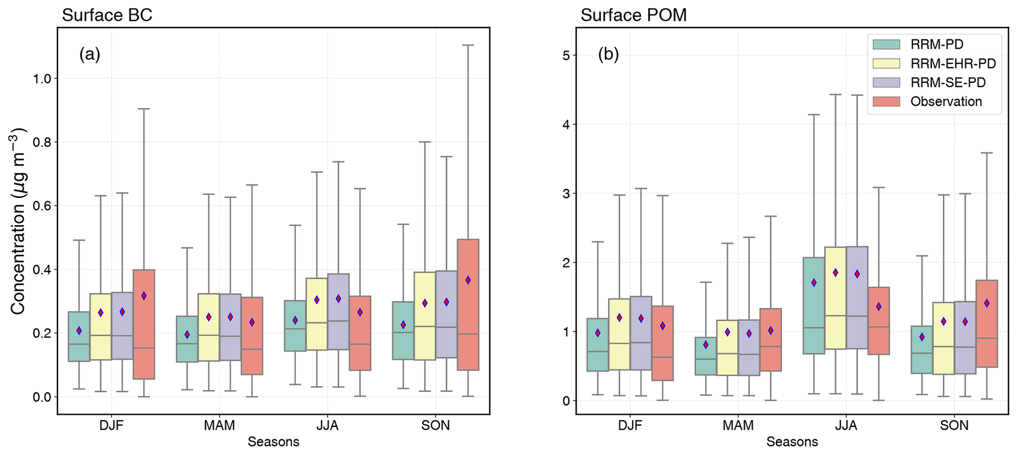
Figure 15 Box plot comparison of the daily mean distribution for (a) BC and (b) POM surface concentrations from RRM-PD simulation, RRM-SE-PD simulation, RRM-EHR-PD simulation, and IMPROVE network measurements. The whiskers are based on 1.5 times the interquartile range (IQR). Distributions are plotted for different seasons over the simulation year, with red diamonds indicating the seasonal means.

Figure 16 Scatter plots between simulated and observed monthly mean surface concentrations of (a, c) sulfate (SO₄) aerosols and (b, d) aerosol optical depth (AOD) at 550 nm. Observations of the surface concentrations and AOD are from IMPROVE and AERONET, respectively, for the simulation year of 2016. Scatter plot statistics compare the Spearman correlation (R), number of data points (n), RMSE, and NMB values between (a, b) RRM-PD, (c, d) RRM-SE-PD, and (e, f) RRM-EHR-PD simulation. RMSE and NMB are defined in Table 2. Solid lines indicate the 1:1 ratio, and the dashed lines indicate the 1:2 and 2:1 ratio. The values at the top of each column indicate the observed mean.

3.4 Impact on the anthropogenic aerosol forcing

As shown in Sect. 3.2, there are large changes in lower-tropospheric aerosol mass concentration and optical properties. Here we evaluate whether the revised emission treatment will affect the anthropogenic aerosol forcing estimate. We calculate the anthropogenic aerosol forcing by taking the difference between simulations with present-day (PD) and pre-industrial (PI) emissions of aerosols and precursors (see Sect. 2.4). We further decompose the aerosol forcing (ΔF) following Ghan (2013) to estimate the forcing caused by aerosol–radiation interaction (or direct aerosol effect, DIR), aerosol–cloud interaction (mainly from indirect aerosol effect, IND), and other residual factors (RES, primarily surface albedo changes).

Figure S17 shows the spatial distribution of decomposed top-of-atmosphere (TOA) ΔF, calculated for the default emission treatment. Over North America (NA), the net aerosol forcing (ΔF) is about −2.4 W m⁻² (Fig. S17a), with the largest contribution from the indirect aerosol effect (IND, Fig. S17d), particularly the shortwave component (ΔF_SW, Fig. S17e). Net longwave aerosol forcing is positive (0.48 W m⁻², Fig. S17c), which is mostly driven by the indirect aerosol effect over ocean (Fig. S17f) and the residual effect over land (Fig. S17o). The direct aerosol effect is very small (−0.035 W m⁻², Fig. S17g).

Figure S18 illustrates the difference in decomposed forcing estimates between the revised and default emission treatments. There are relatively large differences between the original and revised treatments in terms of RMSE. Net aerosol forcing over NA (Fig. S18a) has an RMSE of 1.1 W m⁻², which is mostly driven by the indirect aerosol effect (Fig. S18d). For the annually averaged regional mean anthropogenic aerosol forcing over NA, the relative difference is only about 3 %–5 % between the two treatments. On the other hand, both LR and RRM simulations show structural regional differences over the land and ocean areas (Fig. S19). Therefore, even though the mean differences in the entire NA region are small, the regional/local impact can still be large. Over the subtropical and tropical ocean (mostly away from anthropogenic aerosol emission sources), there are some large neighboring positive and negative differences, which are mostly caused by perturbations (noises) in the cloud fields. This is mainly because the nudging strategy used in this study cannot constrain the large-scale circulation in those areas as efficiently as over the mid-latitude and polar regions (Sun et al., 2019).

4 Conclusions

In this study, we improve the emission treatment in E3SM to better represent the anthropogenic aerosol emission in the simulations. The default E3SM emission treatment fails to preserve spatial heterogeneity or conserve mass, resulting in substantial errors. While using high-resolution emissions can reduce heterogeneity errors, it can incur additional errors due to interpolation and non-conservation over coarser grids. The improved treatment accurately preserves the original spatial heterogeneity and conserves mass both inland and near the coast, providing a more accurate representation of global surface and vertically distributed emissions from coarser to finer model grids. Our results indicate that the default treatment for anthropogenic aerosol emissions in both LR and RRM simulations consistently yields large root mean square errors (RMSE) for all species. The improved emission data prepared for the revised emission treatment can resolve these issues by maintaining spatial heterogeneity and mass conservation. The revised treatment is also applicable to the emission input of other species at different model resolutions.

We find significant differences in the simulated aerosol surface concentration between the default and revised emission treatments. The differences are closely linked to the spatial distribution of prescribed emission gradients, and they persist at higher elevations above the surface. Larger discrepancies are observed in high-frequency concentration profiles. This suggests that errors in default emissions can have a significant impact on the simulated aerosol properties, especially at high resolutions. Consistent with the near-surface mass concentration changes, the default treatment also yields larger errors in simulated extinction and absorption profiles near and above the surface, leading to significant errors in high-frequency aerosol optical depths. This result is particularly relevant, given that short-term high-frequency fields are often used for model evaluations against observations.

Using the default emission treatment can lead to significant errors in aerosol sources and sinks. Substantial errors in the simulated aerosol sources, sinks, and their decomposed components are found along with large relative differences in their spatial distribution. The prescribed emissions and dry deposition are the dominating error terms in BC and POM source–sink components. Errors for wet deposition components for POM and BC were significantly smaller than dry deposition, despite the large fractional contribution to the sink. This is mainly due to the fact that in-cloud scavenging processes do not directly affect prescribed BC and POM in the hydrophobic primary carbon mode upon emission. The largest error contributions for sulfate aerosol sources come from gas–aerosol exchange and in-cloud aqueous-phase chemistry, while wet deposition, particularly stratiform in-cloud scavenging, is the biggest contributor to errors in sinks.

The revised emission treatment leads to improved heterogeneity in simulated surface concentration, particularly in regions with sharp emission gradients. Furthermore, simulations with the revised treatment consistently outperformed simulations with the default treatment in terms of seasonal mean biases and variability of daily mean surface concentrations of black carbon and primary organic matter. Our study highlights the importance of maintaining spatial heterogeneity in aerosol and precursor emissions for high-resolution or variable-resolution model applications.