the Creative Commons Attribution 4.0 License.
the Creative Commons Attribution 4.0 License.
 | 25 Apr 2024
biospheremetrics v1.0.2: an R package to calculate two complementary terrestrial biosphere integrity indicators – human colonization of the biosphere (BioCol) and risk of ecosystem destabilization (EcoRisk)
Johanna Braun
Jannes Breier
Karlheinz Erb
Dieter Gerten
Jens Heinke
Sarah Matej
Sebastian Ostberg
Sibyll Schaphoff
Wolfgang Lucht
Ecosystems are under multiple stressors, and impacts can be measured with multiple variables. Humans have altered mass and energy flows of basically all ecosystems on Earth towards dangerous levels. However, integrating the data and synthesizing conclusions is becoming more and more complicated. Here we present an automated and easy-to-apply R package to assess terrestrial biosphere integrity that combines two complementary metrics.
- (i)
The BioCol metric that quantifies the human colonization pressure exerted on the biosphere through alteration and extraction (appropriation) of net primary productivity.
- (ii)
The EcoRisk metric that quantifies biogeochemical and vegetation structural changes as a proxy for the risk of ecosystem destabilization.
Applied to simulations with the dynamic global vegetation model LPJmL5 for 1500–2016, we find that large regions presently (period 2007–2016) show modification and extraction of >20 % of the preindustrial potential net primary production. The modification (degradation) of net primary production (NPP) as a result of land use change and extraction in terms of biomass removal (e.g., from harvest) leads to drastic alterations in key ecosystem properties, which suggests a high risk of ecosystem destabilization. As a consequence of these dynamics, EcoRisk shows particularly high values in regions with intense land use and deforestation and in regions prone to impacts of climate change, such as the Arctic and boreal zone.
The metrics presented here enable spatially explicit global-scale evaluation of historical and future states of the biosphere and are designed for use by the wider scientific community, being applicable not only to assessing biosphere integrity but also to benchmarking model performance.
The package will be maintained on GitHub and through that we encourage its future application to other models and data sets.
- Article
(15246 KB) - Full-text XML
- BibTeX
- EndNote


Earth system stability relies on functioning ecosystems (McKay et al., 2022), providing, e.g., carbon sequestration, moisture recycling, and resilience to disturbances and disruptions (Friedlingstein et al., 2022; Aragão, 2012; Oliver et al., 2015). The global status and functioning of ecosystems is being evaluated using a range of approaches, including assessments of human footprint (e.g., Venter et al., 2016), indicators based on empirically collected biodiversity data (e.g., Hudson et al., 2017; Newbold et al., 2016), and ecological computer models (e.g., Sakschewski et al., 2015).
Ecosystems depend on photosynthesis as major energy source, producing the primary biomass that is the foundation of almost all food webs. During the Neolithic Revolution, humanity decoupled its biomass demand from the natural cycle, which led to large-scale modification of Earth's surface (Weisdorf, 2005). Today more than 75 % of the ice-free land area of the Earth is affected by human use (Watson et al., 2018; Arneth et al., 2019). However, the level of management and appropriation differs widely from extensive (e.g., occasionally livestock-grazed steppes or extensively used forests) to intensive (e.g., machine-aided agriculture with high mineral fertilizer use and irrigation). The aggregate effect of land use on net primary production (NPP – for a list of all abbreviations see Appendix A), i.e., altered productivity and removed biomass due to agricultural and forestry harvest, is often referred to as the human appropriation of NPP (HANPP) (Haberl et al., 2004; Vitousek et al., 1986; Rojstaczer et al., 2001; Imhoff et al., 2004). Utilizing this concept, it was shown that humanity has doubled its impact during the 20th century and thereby substantially decreased the NPP remaining in ecosystems (Krausmann et al., 2013; Kastner et al., 2022).
As one consequence of land use, only 40 % of remaining forests are still characterized by high ecosystem integrity (Grantham et al., 2020). Globally, only 18.6 % of highly intact habitats are currently protected (Mokany et al., 2020a), while modeling pressure–impact relationships suggest an increasing mean species abundance loss until 2050, even under optimistic scenarios with decreasing land use (Schipper et al., 2020; Williams et al., 2021). Over the course of this century, the dilemma of negative effects from either climate change or climate change mitigation via large-scale biomass plantation highlights the need to also integrate biodiversity in planning for negative emission technologies (Hof et al., 2018).
To prevent further degradation of the biosphere and to reverse the current loss of nature, land use scenarios should take into account the regional risk for ecosystem destabilization (Rockström et al., 2021; Obura et al., 2022). We define ecosystem destabilization as a severe change in ecosystem functioning, resulting in, e.g., a decline in carbon sequestration, species composition, or water provisioning. Shifts in biogeochemical conditions can act as a proxy for this risk based on the argument that substantial changes in either basic biogeochemical properties or vegetation composition are likely to imply far-reaching, potentially self-amplifying transformations in the underlying system characteristics, food chains, and species composition (Heyder et al., 2011). The Γ metric (Gamma) proposed by Heyder et al. (2011) represents such a metric, has been used to separate the historical drivers of ecosystem change (Ostberg et al., 2015), compares the effects of climate warming and land use under future climate scenarios (Ostberg et al., 2018), and finds temperature thresholds above which severe change is to be expected with high probability (Ostberg et al., 2013). Additionally, it has been applied component-wise to model outputs from the ISIMIP fast track ensemble, indicating an increasing area under risk of severe ecosystem change with a rise in global mean temperature (Warszawski et al., 2013).
The original definition of Γ, however, did not include nitrogen variables, and the code to compute it was hardly accessible to the scientific public. HANPP, on the other hand, has so far been based on census statistics and inventory data and has not been calculated purely from vegetation model outputs.
We therefore propose an easy-to-apply R package with two complementary biosphere metrics, BioCol and EcoRisk, building on the existing indicators HANPP and Γ (Haberl et al., 2004; Heyder et al., 2011), which are here exemplarily calculated and evaluated based on simulations with the global vegetation model LPJmL5 (von Bloh et al., 2018).
BioCol quantifies the human colonization pressure on the biosphere through extraction of biomass and prevention of natural NPP by photosynthesis. The metric basically follows the HANPP approach by Haberl et al. (2007), who spatially explicitly sum extracted and inhibited biomass amounts based on biomass inventory data and compare them to potential NPP in a counterfactual world without human land use. We replace biomass inventory data with the corresponding LPJmL5 model outputs and thereby add the possibility of also computing BioCol from deep historical and future simulations.
EcoRisk illustrates state shifts in ecosystems as a result of land, water, and fertilizer use, as well as climate change based on the Γ metric (Heyder et al., 2011; Ostberg et al., 2015). It quantifies, on a scale from 0 (no change) to 1 (very strong change), the dissimilarity of an ecosystem state from a reference condition and comprises four subcomponents (vegetation structure, local change, global importance, ecosystem balance) that are aggregated as a multidimensional proxy for the risk of biosphere destabilization. We follow the original publications but (in addition to water and carbon) now include nitrogen fluxes and pools. The addition of nitrogen variables fills a major gap because nitrogen limitation or surplus is a key determinant for plant growth and the overall ecosystem status.
In this section, we detail the calculation of both BioCol and EcoRisk, our biome classification for spatial aggregation of results, and the relevant specifics of the vegetation model LPJmL5.
2.1 BioCol
We define BioCol (see Fig. 1) as the flow of biomass (in terms of NPP) that is intentionally extracted in the form of crop, residue, and other biomass harvests (NPPharv), plus the inhibited natural biomass production as a result of land use changes, management, and differences in fires (NPPluc). NPPluc is calculated as the difference between potential natural NPP (i.e., the NPP that would prevail without land use but with current climate, Haberl et al., 2014, – NPPpot) and the actual biomass production (NPPact), which are both calculated under the same climate:
Using time series of NPPpot and NPPact allows the removal of the climate change (e.g., CO2 fertilization) effect in the component NPPluc. NPPluc can become negative if the actual NPP is higher than potential NPP (e.g., through management or land use legacy effects, especially on managed grasslands). Absolute HANPP and relative BioCol are computed as
where NPPharv denotes the NPP withdrawn from ecosystems via harvest.
Here NPPref represents a reference NPP. In earlier applications, the respective NPPpot of each year has been used as reference (Kastner et al., 2022; Krausmann et al., 2013). In contrast, here we use NPPref, which refers to the NPPpot of the preindustrial period (mean of 1550–1579), which is the same time frame as for EcoRisk. NPPharv sums the corresponding LPJmL5 model outputs for harvested and extracted carbon from crop areas (including residues), second-generation biomass plantations (not existing in historical period land use input), grassland, timber harvests from land use conversion combined with external timber extraction from managed forests, and human-induced fire carbon emissions. Residue harvest was assumed to contain 70 % of the remaining above-ground biomass after harvest. Carbon extraction of grasslands includes carbon contained in dairy products and methane emissions plus respiration and is based on prescribed livestock densities (Heinke et al., 2023), which are calibrated to match grazing amounts for the year 2000 originally provided by Herrero et al. (2013) and modified by Heinke et al. (2020) (about 1.1 Gt C yr−1 globally). Currently, LPJmL5 is not able to model managed forests and does not separate human-induced and lightning-induced fire carbon emissions. Therefore, timber harvest from managed forests is included as an external dataset from LUH2-v2h (Hurtt et al., 2020). Human-induced fire carbon emissions can be included through external data on the human fire ignition fraction of total fire carbon emissions based on fire models such as LPJmL-Spitfire (Thonicke et al., 2010). For this study, the fire carbon emissions are not included since the updated LPJmL-Spitfire version is still being tested.
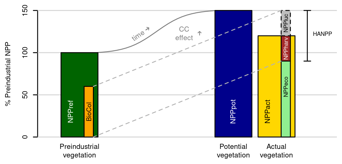
Figure 1Calculation scheme for BioCol. The basis for our analysis is the preindustrial potential NPP (NPPref) assessed from 1550–1579. The effects of CO2 fertilization of plants resulting from historical anthropogenic CO2 emissions, changes in atmospheric N deposition, and climate change lead to a net increase in NPP today (labeled as the “CC effect” in the biosphere) both for hypothetical “potential vegetation” without human land use and the “actual vegetation” including land use. HANPP is calculated as the sum of direct human biomass extraction (NPPharv) and inhibited natural productivity through replacing natural vegetation with land use (). BioCol is subsequently computed as the fraction of HANPP compared to NPPref.
NPPpot, representative of the NPP under potential natural vegetation (under transient climate), is obtained from a model simulation without human land use but with otherwise identical settings to the run providing NPPact. BioCol or HANPP and sub-components are available as spatially explicit values per grid cell for every time step but also as global sums over time, or they are aggregated per biome or world region. When aggregating grid cell values of BioCol, negative values can be treated as such, reducing the overall pressure, or the absolute values of all grid cells can be summed up (which is mainly used in this analysis). For further details on the LPJmL5 simulation setup, see Sect. 2.5.
2.2 EcoRisk
EcoRisk is computed as the average of four subcomponents: vegetation structure (vs), local change (lc), global importance (gi), and ecosystem balance (eb), each on the same scale of 0 to 1 and internally scaled with the respective change-to-variability ratio S(x,σx), following Ostberg et al. (2018).
The unscaled “vegetation structure” component V is evaluated based on the dissimilarity of the vegetation composition of the whole grid cell for both natural and managed areas based on Sykes et al. (1999); Heyder et al. (2011); Ostberg et al. (2018). For this, LPJmL5 provides outputs of the ground area covered by natural and cultivated plant types. Changes in vegetation structure are computed between ecosystem state i and j with respect to the total area (G) of each ground cover type (GCT) k (tree, grass, or barren), further detailed by the differences between the area (A) specific to each plant functional type (PFT, p) regarding attribute l (termed evergreenness, needleleavedness, tropicalness, borealness, and naturalness). For PFT-specific attributes (a), see Table 1. Barren is defined without subcategories. The attribute-specific weighting factor ωkl is per a default value set to 0.2 (= “equal” weighting). Alternatively, attribute-specific weights as in Ostberg et al. (2018) can be applied.
Table 1PFT-specific attributes aklp for GCTs tree and grass.
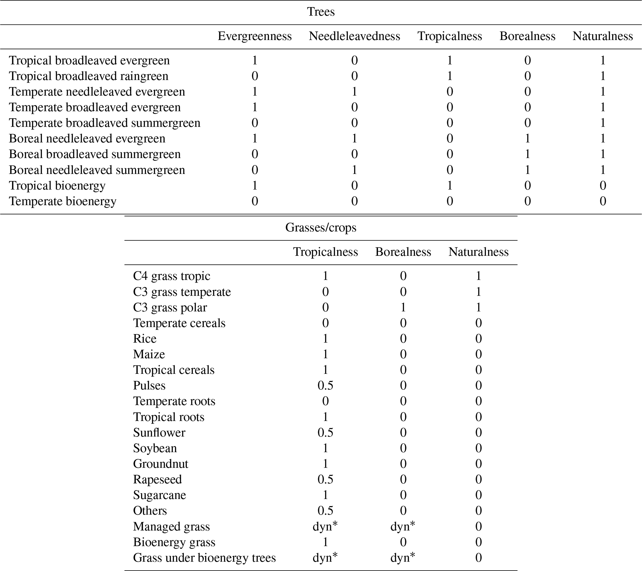
∗ Dynamic share due to climate specific grass mix.
The remaining components l, g, and e are computed from two ecosystem state vectors s1 (reference state) and s2 (changed state), composed of 30-year averages of biogeochemical variables vi,1 and vi,2, with .
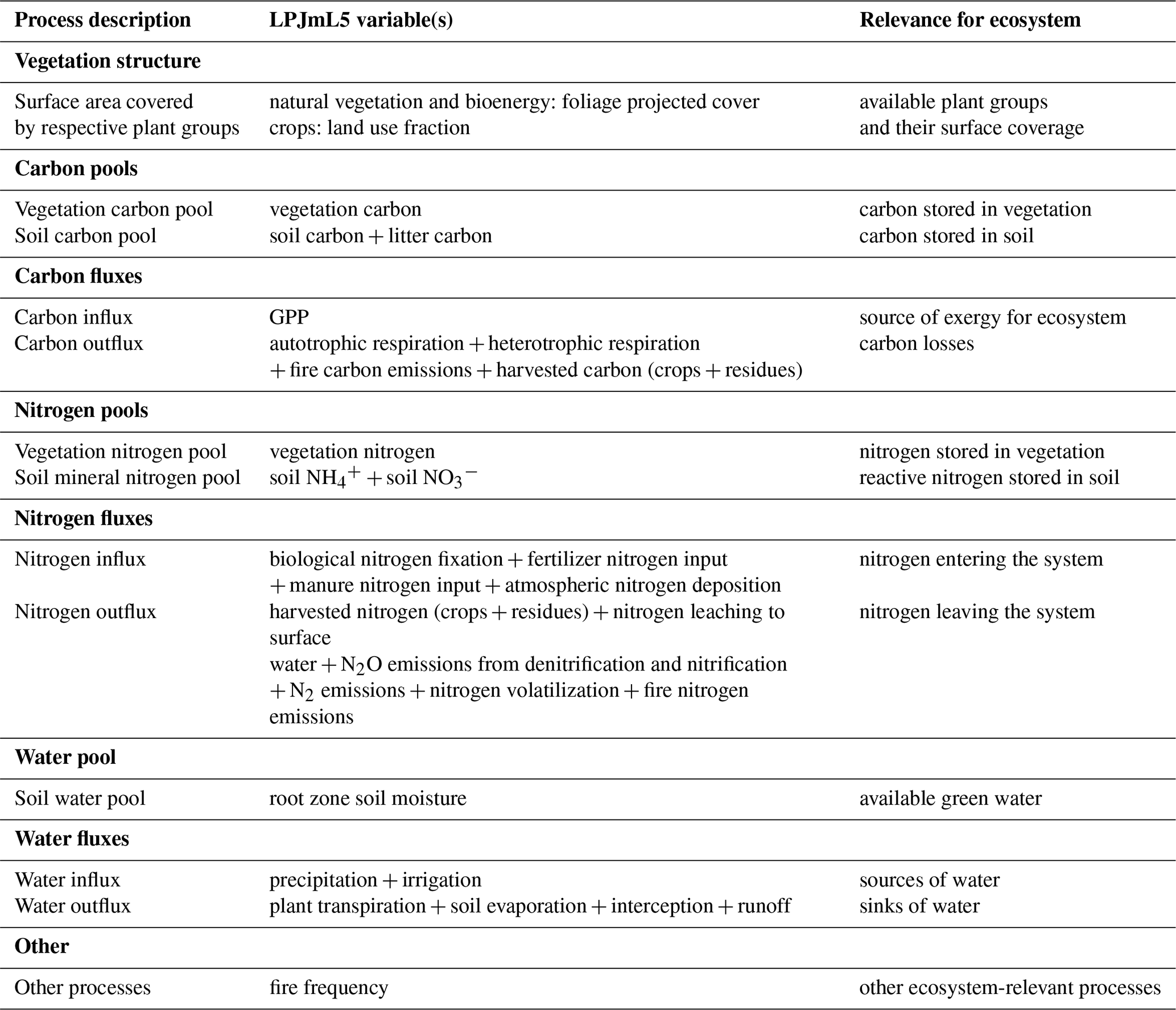
They represent the major process cycles on the grid cell level determining plant growth: carbon, nitrogen, and water. The system described by the metric is the terrestrial land system, which has pools, influxes, and outfluxes across the system boundary. For carbon and nitrogen, stocks are aggregated into a vegetation and soil pool, while for water there is only a soil pool. In total this gives 11 dimensions, plus a single dimension reserved for other relevant processes (for LPJmL filled with the fire frequency) (Table 2). The user can define which model output variables constitute each process dimension. Hereby, it is important to know the model-specific details to keep consistency. If possible, output variables should use per area units because of the per area weighting for the “global importance” component.
Table 2Processes and associated variables describing the land system and their aggregation from LPJmL5 outputs.
“Local change” describes changes compared to the local reference state (e.g., the preindustrial time) as the magnitude change in the difference vector of the biogeochemical properties (how strongly the local conditions have changed). For this, the state variables are normalized with the local values of the reference state:
with
For variables that are 0 in both vectors, both are set to 1, resulting in no change. If only the reference case is 0, the unscaled values are used for both vectors.
“Global importance”, in contrast, puts these local changes in the perspective of the global mean reference condition, taking into account that even moderate changes on the local scale may feed back to larger scales if they are large enough in absolute terms. Therefore, the state vectors are normalized with the global spatially averaged reference mean value :
with
for cells with cell area ap. If the global mean reference state is 0, the mean scenario state is used for scaling instead. If both are 0, both vectors are set to 1, as was done for local change. Afterwards, state vectors for both global importance and local change are multiplied by to scale them down according to the number of variables (EcoRisk can also be computed for simulations without nitrogen, and thus it is missing the corresponding variables). The difference between the two states is now characterized by the length of the difference vector between them, which for local change and global importance are defined as follows:
“Ecosystem balance” quantifies shifts in the relative magnitude of biogeochemical properties with respect to each other as an indicator for qualitative changes in the balance of dynamic processes, which may signal a breakdown of ecological functioning (Ostberg et al., 2018). It is calculated from the angle between the two state vectors with local normalization (as for local change):
b′ is scaled to a range between 0 and 1, assigning a value of 1 if the angle between state vectors is larger than 60°:
Values for metric components l and g are derived by scaling dl and dg to a range between 0 and 1 using the sigmoid transformation function T:
with .
The year-to-year variability is accounted for by the “change-to-variability ratio”. This variability factor is based on the standard deviation (σx) of the component in the 30-year reference period, which is in turn based on the assumption that ecosystems are adapted to the variability they are regularly exposed to but may be vulnerable if it is exceeded. The change-to-variability ratio S(x,σx) for components is calculated as
with σx the interannual standard deviation of x under reference conditions.
For the specific status of variables describing the same process (e.g., carbon pools, or water fluxes), the change metric is also evaluated only for those variables, by default as , but for compatibility with earlier applications it is possible to only use lc.
2.3 Comparison to other indicators
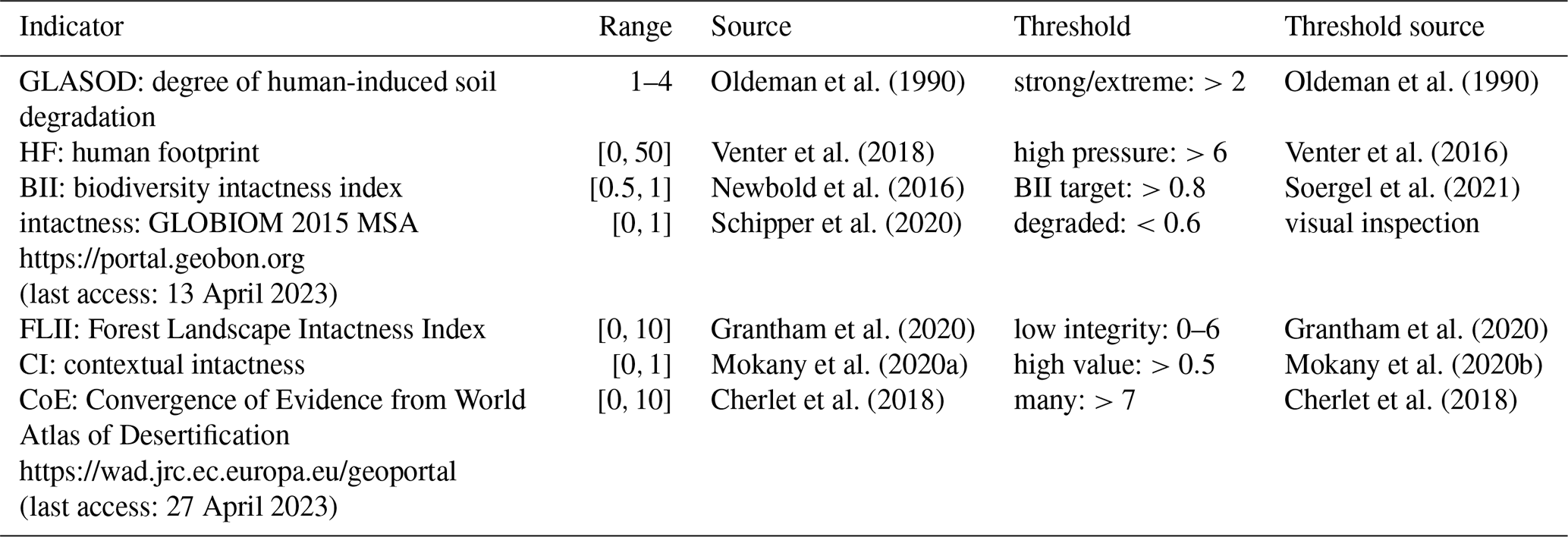
To contextualize EcoRisk and BioCol with other biosphere integrity indicators, we transformed a set of seven widely used biosphere integrity indicators (Table 3) to the interval [0,1] (with 0 meaning high integrity, no pressure, and low risk) and show them alongside EcoRisk and BioCol, together with scatterplots of EcoRisk and BioCol against the average value across all indicators. We additionally extracted thresholds for each indicator from the literature that demarcate the transition between the low- and high-risk zones (sources listed in Table 3). With these we calculated the number of indicators per grid cell that show up as transgressed.
Oldeman et al. (1990)Oldeman et al. (1990)Venter et al. (2018)Venter et al. (2016)Newbold et al. (2016)Soergel et al. (2021)Schipper et al. (2020)Grantham et al. (2020)Grantham et al. (2020)Mokany et al. (2020a)Mokany et al. (2020b)Cherlet et al. (2018)Cherlet et al. (2018)Table 3Sources for other biosphere integrity indicators and associated thresholds.
2.4 Biome classification
To aggregate BioCol and EcoRisk from grid cells to the biome level (to also enable analysis for these larger-scale ecological units), we updated the biome classification for LPJmL5, originally published by Ostberg et al. (2013). It is based on the vegetation structure and its fractional coverage per cell, the tree-specific leaf area index, the temperature, and the carbon stored in vegetation. Cells are classified primarily based on the total tree cover. Thresholds of 60 %, 30 %, and 10 % are chosen to demarcate the boundaries between forests, woody savanna/woodland, savanna, and grassland based on the IGBP land cover classification system (Loveland and Belward, 1997). The dominant tree or grass species then determines the type of biome. Compared to Ostberg et al. (2013), the thresholds can be adjusted and an additional differentiation between Tropical Rainforest and Warm Woody Savanna/Woodland can be either based on the tree leaf area index or the vegetation carbon (in this paper, we use a tree leaf area index of 6 as a threshold). Additionally, Montane Grassland can be differentiated from Arctic Tundra by elevation or latitude (here, we use an elevation threshold of 1000 m).
2.5 LPJmL5
We employ the dynamic global vegetation model LPJmL 5.7 (Schaphoff et al., 2018; von Bloh et al., 2018), which can be run standalone (forced by climate inputs) or coupled into the Potsdam Earth Model POEM (Drüke et al., 2021).
LPJmL5 simulates key ecological and physiological processes such as photosynthesis, respiration, carbon allocation, and turnover for natural and managed vegetation based on historical data or future projections of land use, soil, nitrogen inputs, and climate conditions. The composition of natural vegetation, represented by 11 PFTs, dynamically develops based on climatic parameters, growth efficiency, competition, and fire disturbance (Sitch et al., 2003), while agricultural crop composition is prescribed considering 12 crop functional types (CFTs) (Bondeau et al., 2007), grassland/pastures (Heinke et al., 2023), and three second-generation bioenergy crop functional types (BFTs) (Beringer et al., 2011). The remaining group of “other” crops is simulated as temperate wheat or tropical maize, depending on the latitude. CFT-specific sowing dates are dynamically calculated based on optimal season length and fixed after the year 2000 (Waha et al., 2012). Local runoff is routed through a global network of waterbodies and river channels as accumulated discharge (Gerten et al., 2004). Irrigated crop area is prescribed, but irrigation requirements and water withdrawals are dynamically simulated based on the soil water deficit and available renewable water in lakes, rivers, reservoirs, and neighboring cells with available water (Jägermeyr et al., 2015). Different agricultural management practices and their impacts on soil processes and yields are simulated, including tillage, manure, fertilizer application, and optional growth of off-season cover crops (Lutz et al., 2019; Porwollik et al., 2022). Fluxes and stocks of carbon, nitrogen, and water are by default resolved on 0.5°×0.5° spatial and daily timescale. For this study, all outputs are aggregated per year.
Output from LPJmL5 to compute BioCol and EcoRisk is read and processed using the R package lpjmlkit (Breier et al., 2023).
We ran the model with a fused climate input from the ISIMIP project (GSWP3-W5E5). It combines daily GSWP3 data from 1901 to 1978 with a bias-adjusted version of ERA5 (W5E5, adjusted to better match CRU and GPCC) from 1979 to 2016 (Kim, 2017; Lange, 2019). Manure, fertilizer, and crop-specific cultivation areas from 1500 to 2018 are taken from a new hybrid dataset (Ostberg et al., 2023). Fallow land was included in the CFT class “other”, while the distribution of irrigated area into irrigation systems is based on Jägermeyr et al. (2015). Livestock densities on grasslands were determined based on estimates of grazing levels at both regional and production system levels reported by Herrero et al. (2013) using a set of simulations presented by Heinke et al. (2023). Tillage input is based on Lutz et al. (2019). For simulation years before 1901, the first 30 years of the climate input are randomly recycled.
The results of BioCol are (except for forest harvest) strictly model based and are in general well in line with the existing data-based assessments (Kastner et al., 2022; Krausmann et al., 2013). The global sum of HANPP, based on LPJmL5 simulated outputs, increases from below 2 [2.5] Gt C yr−1 before 1700 to more than 13 [15] Gt C yr−1 today, depending on whether the absolute values are summed up for cells with negative values or not (Fig. 2a – left y axis). Over the course of the 20th century, relative values of BioCol thus approximately doubled from about 0.1 to over 0.2 (10 % to over 20 %) compared to the potential preindustrial NPPref of the 16th century (Fig. 2a – right y axis). Since 2000 the values increased further. When taking the absolute for negative cells, BioCol is approaching 0.25 (25 %) in 2016 – meaning that almost a quarter of the total terrestrial preindustrial biomass production on Earth is rerouted to human use or inhibited compared to a world without humans.
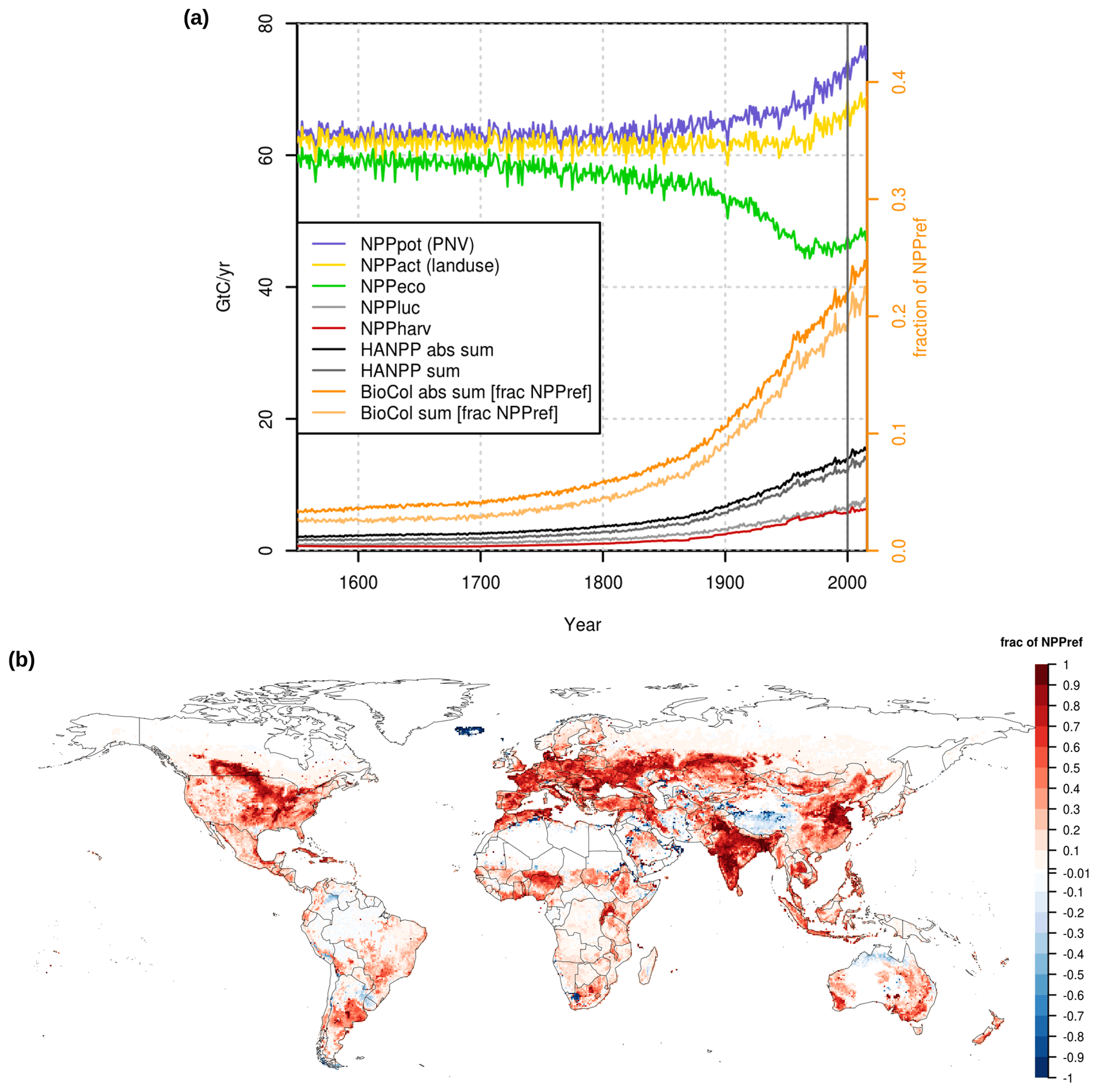
Figure 2(a) Global BioCol and components over time. BioCol values use the orange axis on the right and are calculated as a sum of absolute values (“BioCol abs sum” – cells with negative value increase the global sum) or simple sum (“BioCol sum” – cells with negative value reduce the global sum). (b) Map of the relative values for the year 2000 (average 1995–2005). Relative values for BioCol are expressed in comparison to the average NPP from 1550–1579 from a run without human land use.
The global relative BioCol pattern for the year 2000 (1995–2005 average) shows high values for areas of intense agricultural use (Fig. 2b). The abundance of cells with negative BioCol values (higher productivity in the simulation with land use than in the similar run with only potential natural vegetation) might be explained by the explicit simulation of agricultural management, especially in regions with low natural NPP (e.g., irrigation in the Middle East) and potential legacy effects from earlier land use on now natural areas included in our land use dataset (e.g., in the Amazon, NPP upon regrowth of natural vegetation on abandoned agricultural areas is simulated to be higher than potential NPP in the equilibrium state; see Fig. B1).
Isolated cells with very high absolute BioCol values (e.g., in the boreal zone) are locations of reservoirs established before the year 2005, with associated decline in NPP and thus high values of NPPluc.
EcoRisk calculated between 1550–1579 and 1985–2016 shows large areas with values above 0.5 (Fig. 3), mostly in regions with high land use intensity today. Land use change is reflected in the vegetation structural change component (vs), which quite closely resembles the current land use extent (see inset in Fig. 3). However, the components building on changes in biochemical variables (lc, gi, eb) indicate a much larger extent for regions with values >0.9. Figures 4b and B2 show that in many regions changes in nitrogen fluxes are responsible for these strong changes.
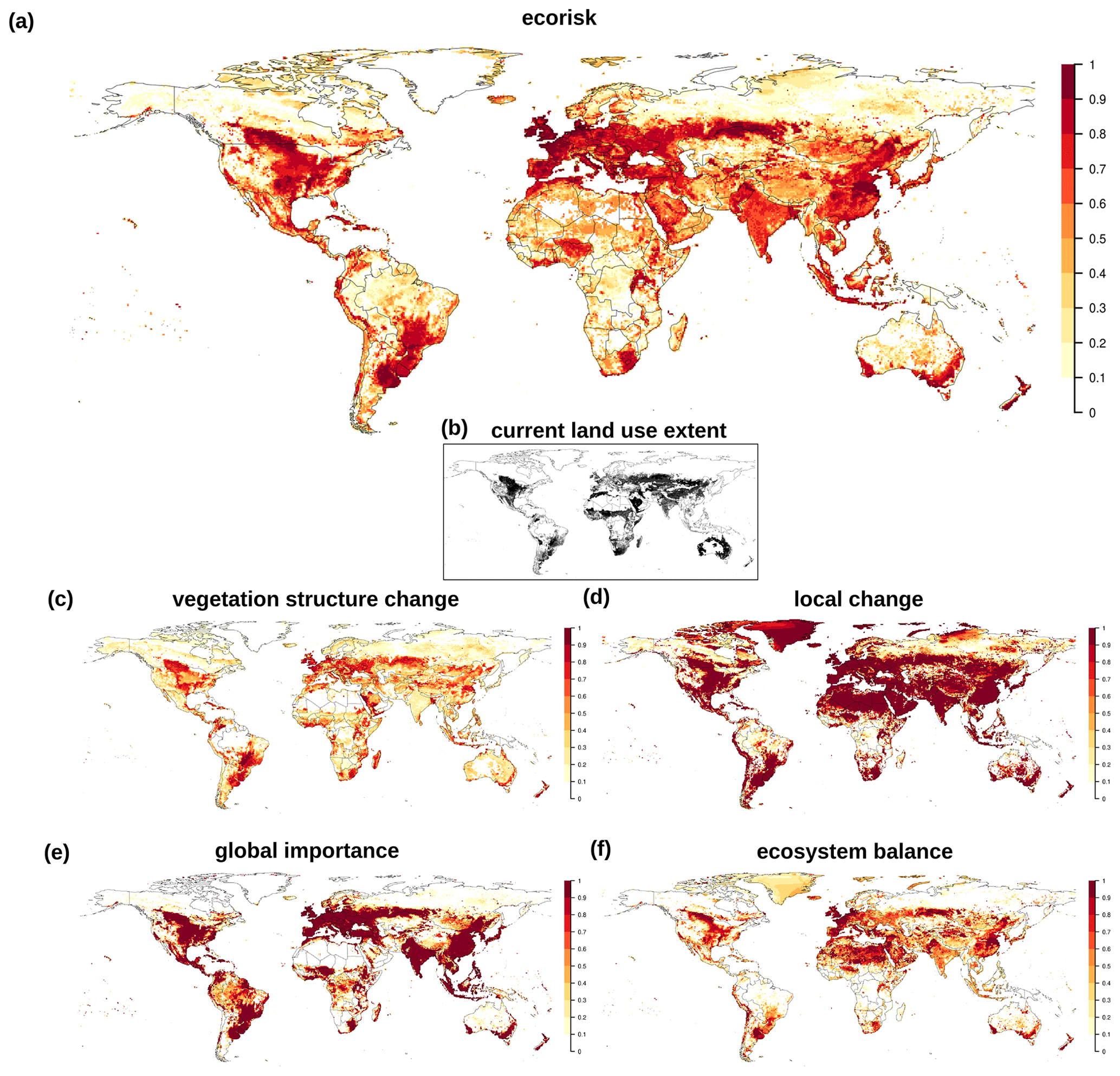
Figure 3(a) Change in biochemical compositions computed by EcoRisk between 1550–1579 and 1985–2016. (b) Current land use extent for reference. (c–f) EcoRisk components are as follows: vegetation structure change, local change, global importance, ecosystem balance.
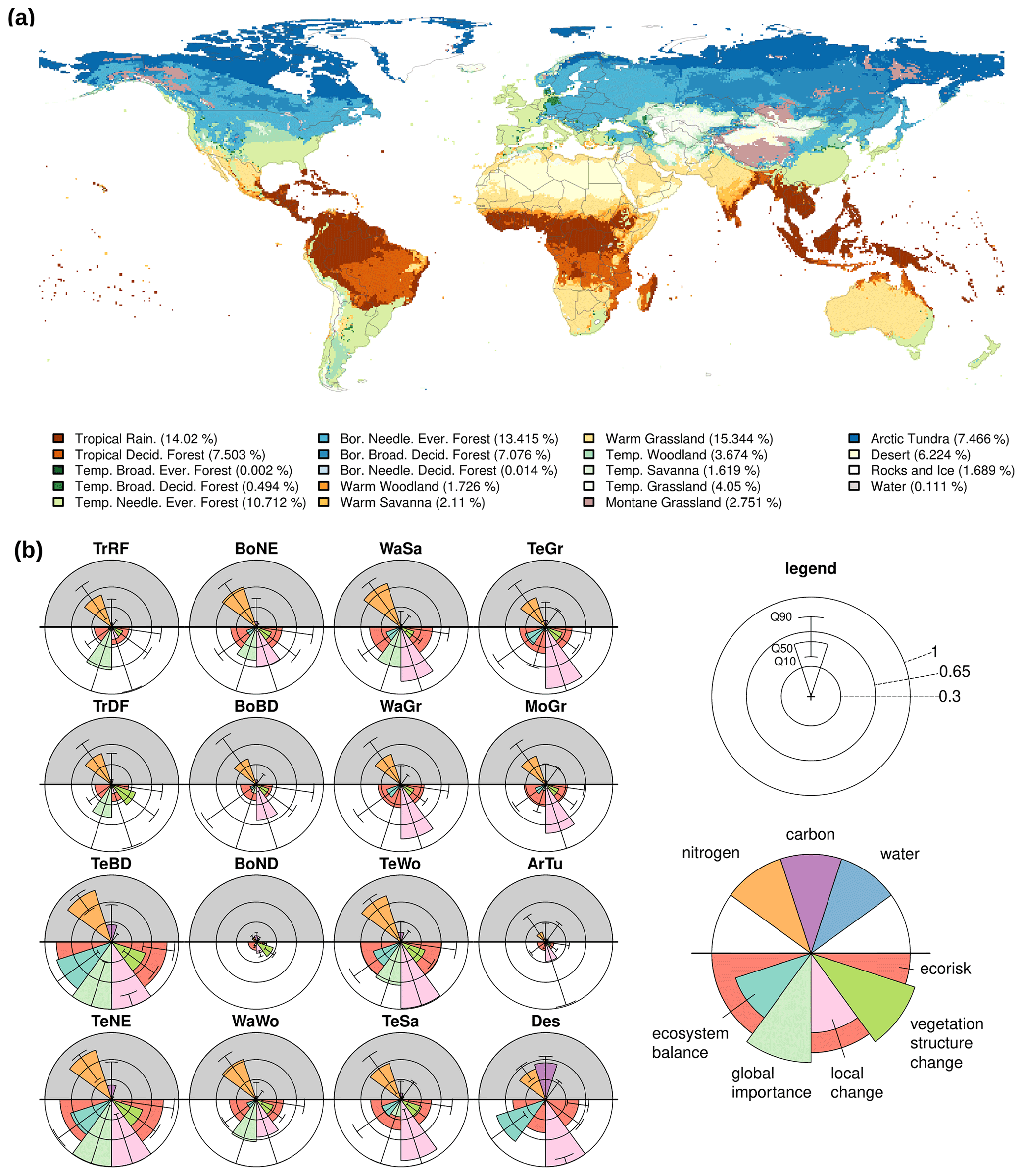
Figure 4(a) Present (1987–2016) biomes classified from vegetation structure, plant-specific leaf area index, temperature and elevation in LPJmL5. (b) Change in biochemical compositions computed by EcoRisk between 1550–1579 and 1985–2016 as the median (Q10 and Q90 for whiskers) across the 16 most relevant biomes (“Temperate Broadleaved Evergreen Forest” is effectively non-existent as only two cells are classified as such, while “Rocks and Ice” and “Water” are skipped for lack of vegetation). See Table B1 for biome names and abbreviations.
Climatic changes are also reflected in EcoRisk. They are most visible in the components ecosystem balance (eb) and vs as bands of higher values along the frontier of boreal vegetation onset to the North in Canada. In Eurasia (and other land-use-free regions of the Arctic) this vegetation shift appears to be more patchy. The local change component (lc) indicates high values among especially vulnerable ecosystems with low absolute values (Arctic, deserts) that do not show up in the global importance (gi). Values of gi are high in regions with strong absolute changes, e.g., with intense land use or loss of tropical rainforests. Ostberg et al. (2018) provides a more detailed discussion of separate and combined effects of land use and climate change (albeit for a somewhat differently defined metric using an earlier model version and different input database).
For the original Γ-metric, a threshold of 0.3 had been established, which indicates the transition from moderate to high risk of ecosystem destabilization. To determine whether this threshold is still valid for EcoRisk (given the adaptations to the computation, particularly the inclusion of nitrogen flows and pools that show more variability), we performed two sets of synthetic simulations. We assume that a meaningful threshold should meet the following two criteria: (i) it should be higher than internal variability within biomes but (ii) lower than the variability between distinct biomes, such that a simulated EcoRisk above this threshold is indicative of changes equivalent to a shift in biome. For (i) we checked the homogeneity within forest biomes by computing EcoRisk with values from 1550–1579 between each cell of a biome and the average cell of this biome. In all forest biomes, internal biome variability for at least half the cells is higher than 0.3 compared to the average biome cell (Fig. B3). Thus, values <0.5 could better describe most of the internal variation.
For (ii), we compared the average biome cells against each other by computing EcoRisk between the current states of each of them. Most combinations show EcoRisk values >0.3 when compared against each other (Fig. B4), with some exceptions: Boreal Needleleaved Evergreen Forest is classified as being relatively similar to Temperate Broadleaved Deciduous Forest (0.26), a fact that we cannot explain and that is also complicated by the reverse direction showing a high value of 0.62. Tropical Rainforest is classified as being similar to Tropical Deciduous Forest. This can be partially explained through their similar locations and the overlap in species. Arctic Tundra and Montane Grassland are classified as being similar. They are in fact the same biome but at different elevations. Comparably, Temperate Savanna, Temperate Woodland, and Warm Grassland are classified as similar biomes that are only differentiated by total tree cover fraction and grass shares. There are further biomes that show intermediate values of when compared against each other, all of which are partially explainable through compositional similarity or similar average conditions.
However, Fig. B4 also highlights that EcoRisk is not symmetric, mainly because of the normalization to different reference conditions for local change and ecosystem balance. Strong directional discrepancies can, for example, be observed for the difference between the three biomes Temperate Needleleaved Evergreen Forest, Temperate Broadleaved Deciduous Forest, and Boreal Needleleaved Evergreen Forest.
Aggregating EcoRisk grid cell values to the biome level according to the biome classification yields three classes (Fig. 4): (i) those with a median EcoRisk<0.3, i.e., Tropical Rainforest, Tropical Deciduous Forest, Boreal Broadleaved Deciduous Forest, Boreal Needleleaved Deciduous Forest (only few cells), and Arctic Tundra; (ii) those with , i.e., Boreal Needleleaved Evergreen Forest, Warm Woodland, Warm Savanna, Warm Grassland, Temperate Savanna, Temperate Grassland, Montane Grassland, and Desert; and (iii) those with a median EcoRisk>0.65, i.e., Temperate Broadleaved Deciduous Forest, Temperate Needleleaved Evergreen Forest, and Temperate Woodland. The subcomponent local change is generally the one with highest values (except for TrRF, TrDF, and BoND), and nitrogen fluxes show stronger changes than those for carbon and water in all cases.
Comparison of EcoRisk and BioCol with other biosphere integrity indicators (Table 3) shows similar trends despite high scattering (Fig. 5k and m). The maps highlight that the pattern of BioCol is more similar to that of other transgressed indicators (Fig. 5a–j); however, this might stem from most of them being directly affected by land use. The additional benefit of EcoRisk is that it also captures effects due to climate and deposition changes.
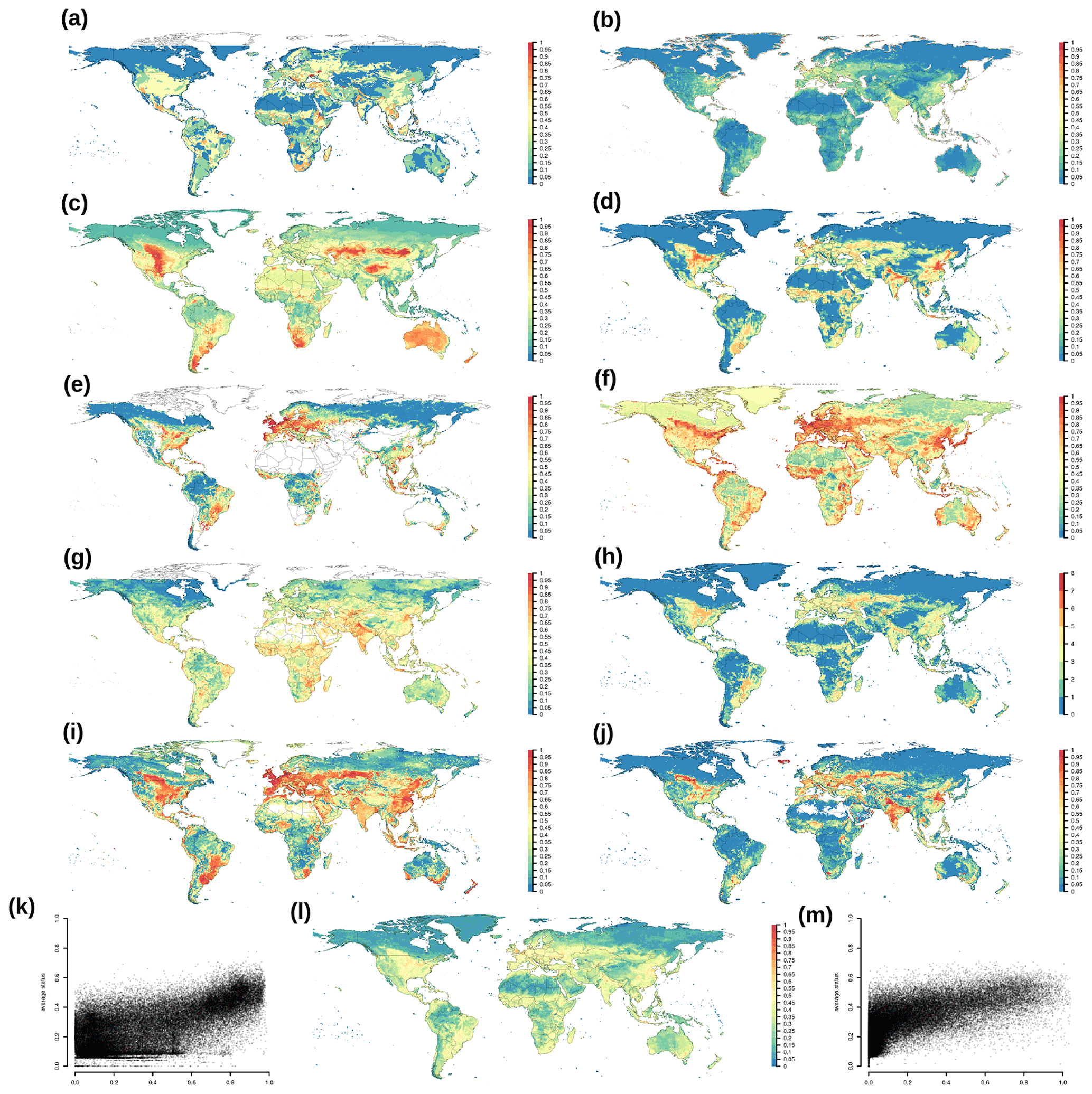
Figure 5Contextualization of several indicators of biosphere integrity, transformed to the interval [0,1], with 0 meaning high integrity, no pressure, and low risk: (a) GLASOD representing human-induced soil degradation (Oldeman et al., 1990), (b) HF representing human footprint (Venter et al., 2016), (c) BII representing the biodiversity intactness index (Newbold et al., 2016), (d) intactness representing GLOBIOM 2015 MSA (Schipper et al., 2020), (e) FLII representing the Forest Landscape Intactness Index (Grantham et al., 2020), (f) CI representing contextual intactness (Mokany et al., 2020b), (g) CoE representing the Convergence of Evidence from World Atlas of Desertification (Cherlet et al., 2018). (h) The number of the previous seven indicators that show up as transgressed per grid cell (see Table 3 for thresholds indicating transition between low- and high-risk zones), (i) EcoRisk and (j) BioCol (l) average of metrics shown in (a)–(g), (k) scatterplot of EcoRisk versus average, and (m) scatterplot of BioCol versus average.
We present a model-based indicator set that allows for the assessment of the state of the biosphere. We show that large regions presently (period 2007–2016) show modification and extraction of >20 % of the preindustrial potential net primary production according to the indicator BioCol, along with climatic changes leading to drastic alterations in key ecosystem properties and suggesting a high risk of ecosystem destabilization according to the indicator EcoRisk.
Generally, the indicators presented in this package can serve both as an analytic tool to assess biosphere integrity from model simulations or as a means of benchmarking model performance (e.g., after new development). Therefore, depending on the context, the performance of the vegetation model is important. This paper primarily describes the methodology behind the biospheremetrics package, with the application to model results only being secondary. LPJmL5 is currently in a recalibration and validation phase, with major changes to code and key processes, following the implementation of tillage and the nitrogen cycle. Further model development may particularly focus on an improved distribution of PFTs and thus biomes (see Harper et al., 2023 for comparison) and the explicit simulation of multi-cropping, which has been neglected here. A better representation of human-induced fire emissions and including process-based forest management will also be important, since the effects on NPP are currently not considered.
The next step for us is thus to extend the biospheremetrics package to be compatible with other vegetation models (e.g., utilizing outputs from the ISIMIP3 ensemble) and thus also allow for intermodel comparison.
As presented in the previous section, the addition of nitrogen fluxes leads to a strong increase in values for EcoRisk, when compared to earlier results of the Γ-Metric (Figs. 3 and B2 and Ostberg et al., 2015, 2018). Relative changes in nitrogen fluxes (Fig. B5) as a result of nitrogen fertilizer and manure application are much stronger than those for carbon and water fluxes and pools (Figs. B6 and 4). This is intuitively plausible; however, the question remains, whether the associated high values for EcoRisk mainly resulting from the relative changes in nitrogen fluxes really correspond to a strongly increased risk for ecosphere destabilization. Generally, a theory of how changes in different components (vs, lc, gi, eb) or classes of state variables (e.g., water pools or nitrogen fluxes) can be translated to risk of ecosphere destabilization is lacking (and could be different among components and classes). Theoretically, a weighted downscaling of any component would be possible; however, the literature base for such changes is currently lacking. We thus refrained from any weighting until further research is done on this end.
The results for EcoRisk show a strong increase in the overall values. A new threshold between moderate and high risk (replacing 0.3 in Ostberg et al., 2018, 2015; Heyder et al., 2011) would be as high as 0.48, when picking the “optimal” EcoRisk threshold, balancing between forest biome internal homogeneity on the one hand and inter-biome dissimilarity on the other hand (Fig. B7).
Our way to calculate BioCol differs substantially from previous approaches for HANPP. First, our calculation is exclusively based on model output, with the aim to also simulate future scenarios and historical periods outside of available biomass inventory data. However, we also use a different baseline when comparing it to the static preindustrial NPP and taking the absolute of cells with negative HANPP values. Both processes are done deliberately in order to (i) not let ourselves get distracted from the fact that global NPP is mainly rising because the biosphere is in a resilience response phase to increasing atmospheric CO2 levels, meaning that this additional NPP is not ours to use, and (ii) acknowledge that management-driven NPP increases beyond the potential natural values (negative NPPluc) usually go together with modification of the water, carbon, or nitrogen cycles stressing local ecosystems.
The underlying principle of BioCol, NPP appropriation, is a function of human demand, i.e., land use change and biomass harvesting for food, fiber, fodder, bioenergy, and bioeconomy. It is therefore closely associated with issues not just of Earth system stability but also of justice, access, and sustainable management of resources (see Gupta et al., 2023). The challenge is to maintain the productivity of the biosphere, i.e., the sustainably available NPP, while ensuring the stability of the biosphere and also including climate and the ecosphere, i.e., the Earth system as used by humans.
Complementarily, EcoRisk indicates where and when critical transitions in ecosystems occur (as a result of NPP appropriation, but also from climate change, or other environmental pollution). It is thus a very useful indicator to assess the risk of ecosystem destabilization today and also going forward, depending on which pathway humanity will take in the future. We deliberately call it a risk metric because the mathematical property of measuring a non-directional change for us directly translates to a proxy for the risk of ecosystem destabilization. Of course there could be regions where ecosystems can benefit from changing biogeochemical properties; however, we would argue that when comparing to a long-term stable, land-use-free preindustrial reference situation (like the Holocene), most ecosystems would be at the risk of being thrown out of this equilibrium when presented with changing conditions. This choice of reference might need to be changed for application of EcoRisk to future climate stabilization scenarios with “Earth-System Stewardship” (Rockström et al., 2021; Steffen et al., 2018).
Humanity faces the challenge of stabilizing the Earth system in the Anthropocene. This requires stabilizing the climate and maintaining a resilient biosphere, which represents, according to Steffen et al. (2015), a key pillar of the Earth system. Here we present two computable biosphere integrity indicators that allow for the assessment of the historical and future risk of biosphere destabilization. These are designed to complement other biosphere integrity indicators.
Human appropriation of NPP is a direct result of land use changes, modulated by climatic changes, irrigation, fertilization, and other management, leading to biosphere integrity loss that can be measured by EcoRisk. On the other hand, natural NPP is also modified by changes in climate, water availability, biosphere integrity, and human land use. Thus, BioCol and EcoRisk are metrics that integrate multiple terrestrial planetary boundaries (Rockström et al., 2009; Steffen et al., 2015) and human drivers into two numbers, comparable to what global mean temperature does for the underlying more complex climate processes. Therefore, BioCol and EcoRisk have the potential to be included as indicators in an updated planetary boundaries framework. While well established as a concept, so far there has been no simulation model for assessing and projecting HANPP on the global scale for example to analyze future scenarios not accessible through inventory data.
Both BioCol and EcoRisk are spatially explicit, process-based, and computable metrics that can be aggregated over space and time. They can therefore serve as integrative meta-level proxies for biosphere integrity and Earth system stability and their dynamic changes. The code used here for their calculation is distributed as an open-source R package, and we invite external contributions. With the next update, we plan to equip it to deal with netcdf files, a common data exchange format for spatial data, which allows for future application to different models. Thereby, we hope to encourage others to join our quest to better understand the role of ecosystems for Earth system stability and find ways to preserve it.
| BFT | Bioenergy functional type |
| CFT | Crop functional type |
| GCT | Ground cover type |
| HANPP | Human appropriation of NPP |
| LPJmL | Lund–Potsdam–Jena managed Land |
| (a dynamic global vegetation model) | |
| BioCol | Metric for human biomass colonization pressure |
| EcoRisk | Metric for risk of ecosystem destabilization |
| NPP | Net primary production |
| PFT | Plant functional type |
Table B1Names and abbreviations for all biomes according to our biome classification.
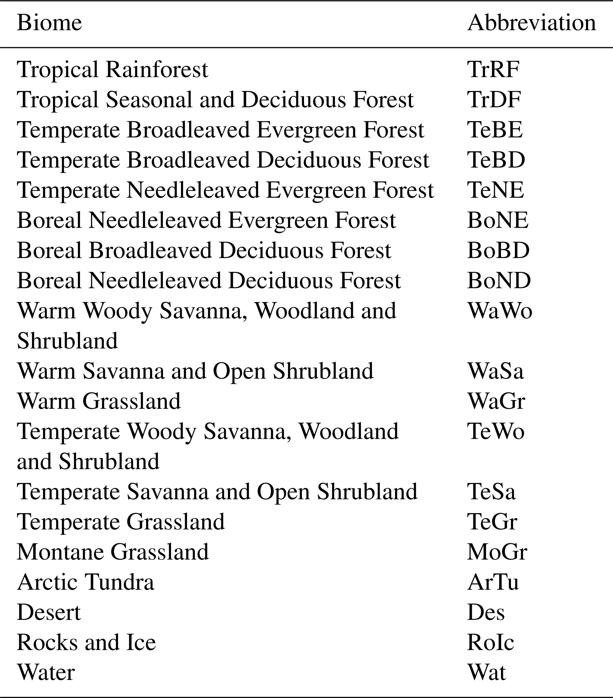
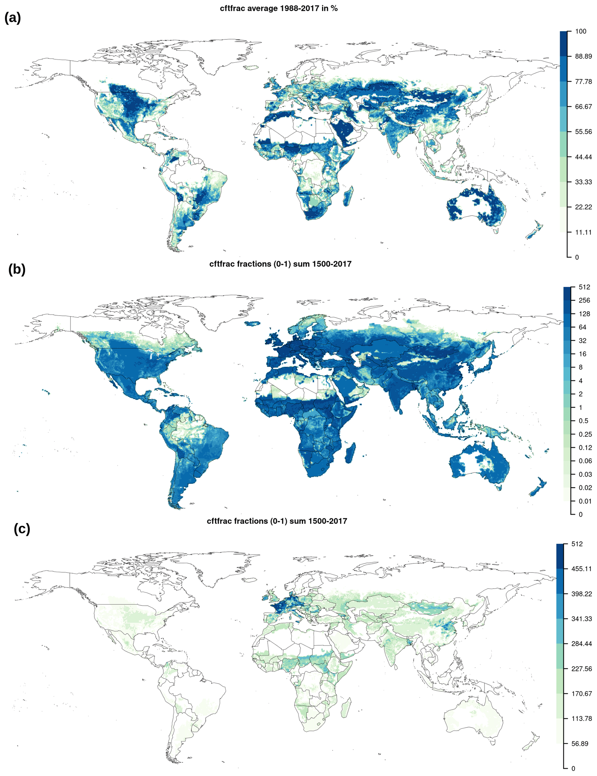
Figure B1(a) Average land use between 1988–2017 in percentage of grid cell area. Total historical sum of yearly land use fractions [0–1] with an (b) exponential and (c) linear legend.

Figure B2(a) Change in biochemical compositions computed by EcoRisk (as in Fig. 3, but excluding nitrogen variables) between 1550–1579 and 1985–2016. (b–e) EcoRisk components, i.e., vegetation structure change, local change, global importance, and ecosystem balance.
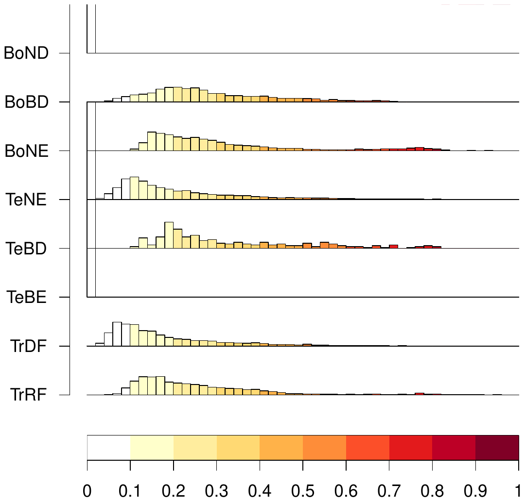
Figure B3Biome internal difference distribution for the forest biomes computed using EcoRisk between each cell of the biome with the average cell of the biome (for 1550–1579 states). Note that only very few cells are classified as BoND or TeBE; therefore, their distribution appears very homogeneous. For biome names and abbreviations, see Table B1.
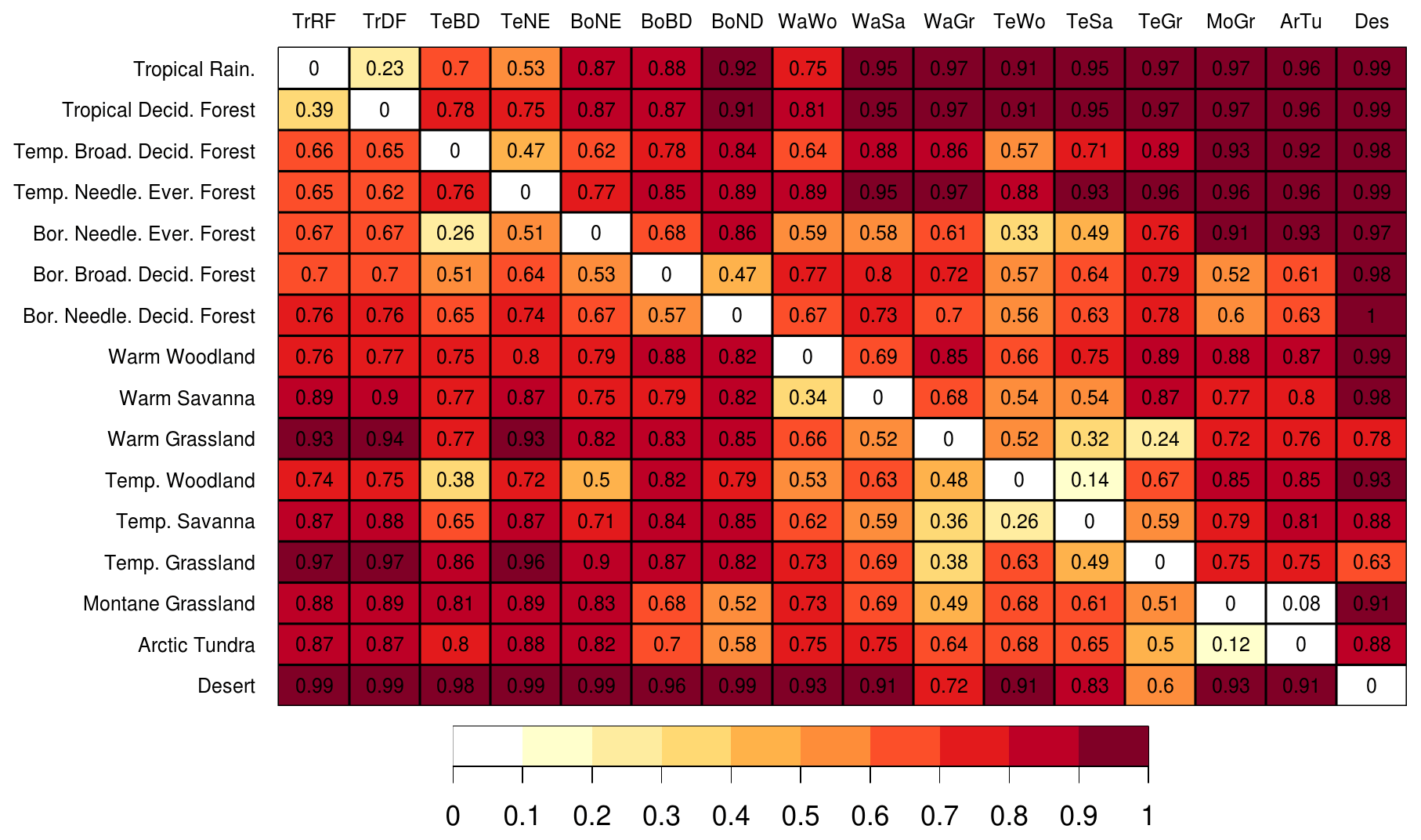
Figure B4Comparison of the state difference (EcoRisk) between biomes according to the average biome cell (y: reference state; x: scenario state) evaluated for the average state of 1550–1579. The color code is the same as in Fig. B3. Since only very few cells are classified as TeBE, this biome is left out. Biomes RoIce and Wat do not host vegetation and are also left out. For biome names and abbreviations, see Table B1.
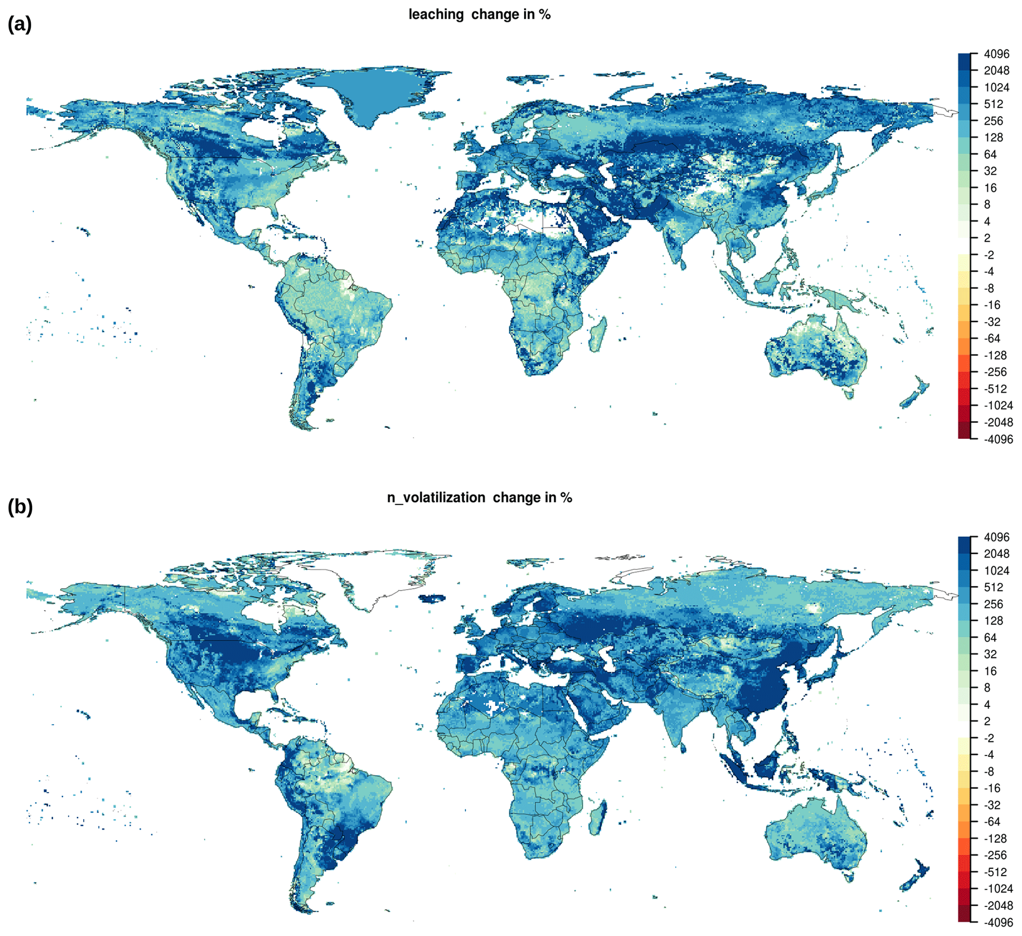
Figure B5Change in (a) leaching and (b) nitrogen volatilization between 1550–1579 and 1985–2016.
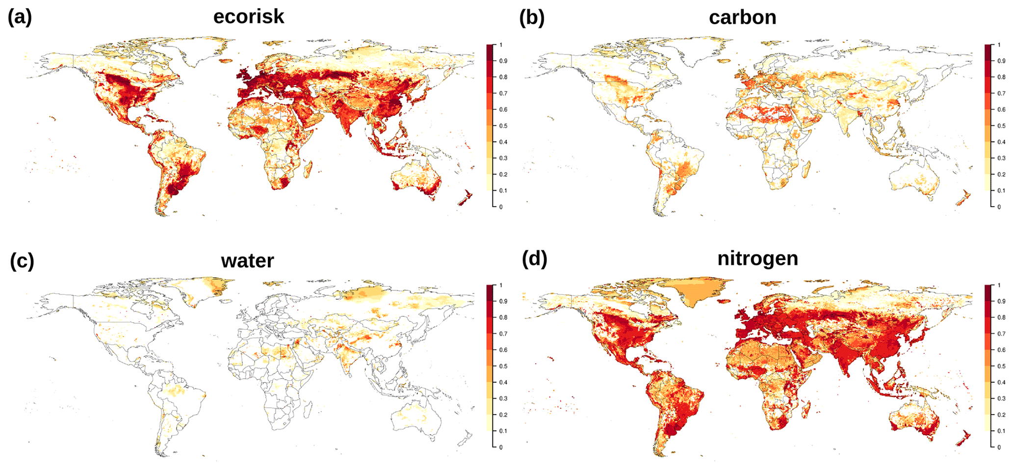
Figure B6Change in biochemical compositions computed by EcoRisk between 1550–1579 and 1985–2016. (a) Total EcoRisk and an evaluation of for only components related to (b) carbon, (c) water, and (d) nitrogen.
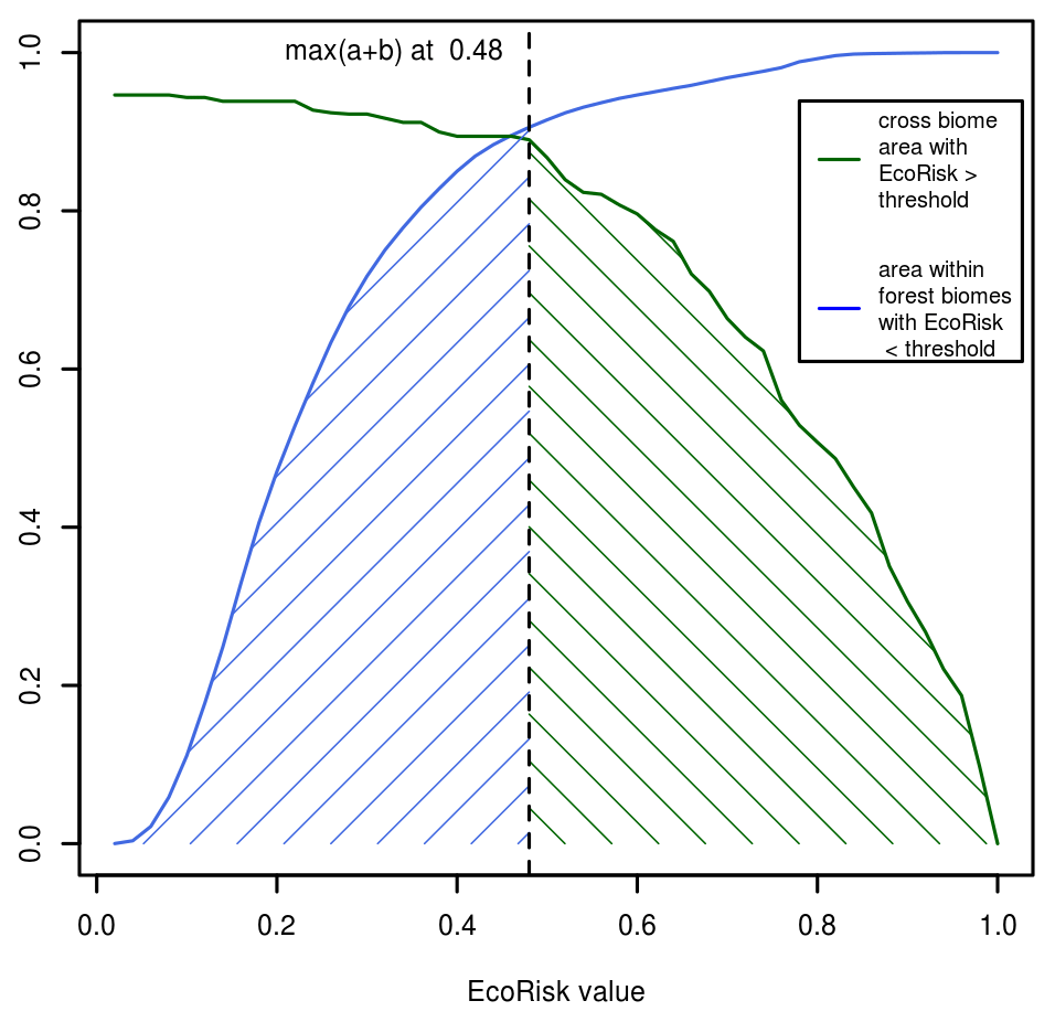
Figure B7Cumulative area for all cells defined as not similar (EcoRisk > threshold) according to Fig. B4 (green) and defined as similar (EcoRisk < threshold) to the biome average according to Fig. B3 (blue). The value where the sum of both curves is maximal (an optimal threshold value fulfilling both criteria) is indicated by the dashed vertical line.
The package is available via GitHub https://github.com/stenzelf/biospheremetrics (last access: 6 March 2024), and it is permanently archived via Zenodo https://doi.org/10.5281/zenodo.10699198 (Stenzel, 2024). LPJmL model code, simulation data, and scripts to generate the figures are available on Zenodo https://doi.org/10.5281/zenodo.10008051 (Stenzel, 2023).
FS: conceptualization, methodology, software, validation, formal analysis, writing – original draft, visualization. JoB: methodology, software, writing – review and editing. JaB: software, writing – review and editing. KE: methodology, writing – review and editing. DG: writing – review and editing, supervision. JH: software (livestock–grassland calibration implementation). SM: methodology, data curation, writing – review and editing. SO: methodology, software, writing – review and editing. SiS: conceptualization, data curation, writing – review and editing. WL: conceptualization, writing – review and editing, supervision, funding acquisition.
The contact author has declared that none of the authors has any competing interests.
Publisher's note: Copernicus Publications remains neutral with regard to jurisdictional claims made in the text, published maps, institutional affiliations, or any other geographical representation in this paper. While Copernicus Publications makes every effort to include appropriate place names, the final responsibility lies with the authors.
We thank the Ecosystem in Transitions group at PIK and especially Boris Sakschewski for providing fruitful discussions.
This research has been supported by the Global Challenges Foundation through the Future Earth project fund “New Governance Architecture for Addressing Global Systemic Risks”. Jens Heinke received financial support from ESM2025 (grant no. 101003536).
The publication of this article was funded by the Open Access Fund of the Leibniz Association.
This paper was edited by Carlos Sierra and reviewed by Juan Rocha and one anonymous referee.
Aragão, L. E. O. C.: The rainforest's water pump, Nature, 489, 217–218, https://doi.org/10.1038/nature11485, 2012. a
Arneth, A., Denton , F., Agus, F., Elbehri, A., Erb, K. H., Osman Elasha, B., Rahimi, M., Rounsevell, M., Spence, A., Valentini, R., and Debonne, N.: Framing and Context, in: Climate Change and Land: an IPCC special report on climate change, desertification, land degradation, sustainable land management, food security, and greenhouse gas fluxes in terrestrial ecosystems, Intergovernmental Panel on Climate Change (IPCC), 1–98, https://www.ipcc.ch/site/assets/uploads/2019/08/2b.-Chapter-1_FINAL.pdf (11 April 2024), 2019. a
Beringer, T., Lucht, W., and Schaphoff, S.: Bioenergy production potential of global biomass plantations under environmental and agricultural constraints, GCB Bioenergy, 3, 299–312, https://doi.org/10.1111/j.1757-1707.2010.01088.x, 2011. a
Bondeau, A., Smith, P. C., Zaehle, S., Schaphoff, S., Lucht, W., Cramer, W., Gerten, D., Lotze-Campen, H., Müller, C., Reichstein, M., and Smith, B.: Modelling the role of agriculture for the 20th century global terrestrial carbon balance, Global Change Biol., 13, 679–706, https://doi.org/10.1111/j.1365-2486.2006.01305.x, 2007. a
Breier, J., Ostberg, S., Wirth, S. B., Minoli, S., Stenzel, F., and Müller, C.: lpjmlkit: Toolkit for Basic LPJmL Handling, https://doi.org/10.5281/zenodo.7773134, 2023. a
Cherlet, M., Hutchinson, C., Reynolds, J., Hill, J., Sommer, S., and Von Maltitz, G. E.: World atlas of desertification: rethinking land degradation and sustainable land management, Publication Office of the European Union, Luxembourg, https://doi.org/10.2760/06292, 2018. a, b, c
Drüke, M., von Bloh, W., Sakschewski, B., Wunderling, N., Petri, S., Cardoso, M., Barbosa, H. M. J., and Thonicke, K.: Climate-induced hysteresis of the tropical forest in a fire-enabled Earth system model, Eur. Phys. J.-Spec. Top., 230, 3153–3162 https://doi.org/10.1140/epjs/s11734-021-00157-2, 2021. a
Friedlingstein, P., O'Sullivan, M., Jones, M. W., Andrew, R. M., Gregor, L., Hauck, J., Le Quéré, C., Luijkx, I. T., Olsen, A., Peters, G. P., Peters, W., Pongratz, J., Schwingshackl, C., Sitch, S., Canadell, J. G., Ciais, P., Jackson, R. B., Alin, S. R., Alkama, R., Arneth, A., Arora, V. K., Bates, N. R., Becker, M., Bellouin, N., Bittig, H. C., Bopp, L., Chevallier, F., Chini, L. P., Cronin, M., Evans, W., Falk, S., Feely, R. A., Gasser, T., Gehlen, M., Gkritzalis, T., Gloege, L., Grassi, G., Gruber, N., Gürses, Ö., Harris, I., Hefner, M., Houghton, R. A., Hurtt, G. C., Iida, Y., Ilyina, T., Jain, A. K., Jersild, A., Kadono, K., Kato, E., Kennedy, D., Klein Goldewijk, K., Knauer, J., Korsbakken, J. I., Landschützer, P., Lefèvre, N., Lindsay, K., Liu, J., Liu, Z., Marland, G., Mayot, N., McGrath, M. J., Metzl, N., Monacci, N. M., Munro, D. R., Nakaoka, S.-I., Niwa, Y., O'Brien, K., Ono, T., Palmer, P. I., Pan, N., Pierrot, D., Pocock, K., Poulter, B., Resplandy, L., Robertson, E., Rödenbeck, C., Rodriguez, C., Rosan, T. M., Schwinger, J., Séférian, R., Shutler, J. D., Skjelvan, I., Steinhoff, T., Sun, Q., Sutton, A. J., Sweeney, C., Takao, S., Tanhua, T., Tans, P. P., Tian, X., Tian, H., Tilbrook, B., Tsujino, H., Tubiello, F., van der Werf, G. R., Walker, A. P., Wanninkhof, R., Whitehead, C., Willstrand Wranne, A., Wright, R., Yuan, W., Yue, C., Yue, X., Zaehle, S., Zeng, J., and Zheng, B.: Global Carbon Budget 2022, Earth Syst. Sci. Data, 14, 4811–4900, https://doi.org/10.5194/essd-14-4811-2022, 2022. a
Gerten, D., Schaphoff, S., Haberlandt, U., Lucht, W., and Sitch, S.: Terrestrial vegetation and water balance–hydrological evaluation of a dynamic global vegetation model, J. Hydrol., 286, 249–270, https://doi.org/10.1016/j.jhydrol.2003.09.029, 2004. a
Grantham, H. S., Duncan, A., Evans, T. D., Jones, K. R., Beyer, H. L., Schuster, R., Walston, J., Ray, J. C., Robinson, J. G., Callow, M., Clements, T., Costa, H. M., DeGemmis, A., Elsen, P. R., Ervin, J., Franco, P., Goldman, E., Goetz, S., Hansen, A., Hofsvang, E., Jantz, P., Jupiter, S., Kang, A., Langhammer, P., Laurance, W. F., Lieberman, S., Linkie, M., Malhi, Y., Maxwell, S., Mendez, M., Mittermeier, R., Murray, N. J., Possingham, H., Radachowsky, J., Saatchi, S., Samper, C., Silverman, J., Shapiro, A., Strassburg, B., Stevens, T., Stokes, E., Taylor, R., Tear, T., Tizard, R., Venter, O., Visconti, P., Wang, S., and Watson, J. E. M.: Anthropogenic modification of forests means only 40 % of remaining forests have high ecosystem integrity, Nat. Commun., 11, 5978, https://doi.org/10.1038/s41467-020-19493-3, 2020. a, b, c, d
Gupta, J., Liverman, D., Prodani, K., Aldunce, P., Bai, X., Broadgate, W., Ciobanu, D., Gifford, L., Gordon, C., Hurlbert, M., Inoue, C. Y. A., Jacobson, L., Kanie, N., Lade, S. J., Lenton, T. M., Obura, D., Okereke, C., Otto, I. M., Pereira, L., Rockström, J., Scholtens, J., Rocha, J., Stewart-Koster, B., David Tàbara, J., Rammelt, C., and Verburg, P. H.: Earth system justice needed to identify and live within Earth system boundaries, Nature Sustainability, 6 630–638, https://doi.org/10.1038/s41893-023-01064-1, 2023. a
Haberl, H., Erb, K.-H., Krausmann, F., and Lucht, W.: Defining the human appropriation of net primary production, LUCC Newsletter, 10, 16–17, 2004. a, b
Haberl, H., Erb, K. H., Krausmann, F., Gaube, V., Bondeau, A., Plutzar, C., Gingrich, S., Lucht, W., and Fischer-Kowalski, M.: Quantifying and mapping the human appropriation of net primary production in earth's terrestrial ecosystems, P. Natl. Acad. Sci. USA, 104, 12942–12947, https://doi.org/10.1073/pnas.0704243104, 2007. a
Haberl, H., Erb, K.-H., and Krausmann, F.: Human Appropriation of Net Primary Production: Patterns, Trends, and Planetary Boundaries, Annu. Rev. Env. Resour., 39, 363–391, https://doi.org/10.1146/annurev-environ-121912-094620, 2014. a
Harper, K. L., Lamarche, C., Hartley, A., Peylin, P., Ottlé, C., Bastrikov, V., San Martín, R., Bohnenstengel, S. I., Kirches, G., Boettcher, M., Shevchuk, R., Brockmann, C., and Defourny, P.: A 29 year time series of annual 300 m resolution plant-functional-type maps for climate models, Earth Syst. Sci. Data, 15, 1465–1499, https://doi.org/10.5194/essd-15-1465-2023, 2023. a
Heinke, J., Lannerstad, M., Gerten, D., Havlík, P., Herrero, M., Notenbaert, A. M. O., Hoff, H., and Müller, C.: Water Use in Global Livestock Production–Opportunities and Constraints for Increasing Water Productivity, Water Resour. Res., 56, e2019WR026995, https://doi.org/10.1029/2019WR026995, 2020. a
Heinke, J., Rolinski, S., and Müller, C.: Modelling the role of livestock grazing in C and N cycling in grasslands with LPJmL5.0-grazing, Geosci. Model Dev., 16, 2455–2475, https://doi.org/10.5194/gmd-16-2455-2023, 2023. a, b, c
Herrero, M., Havlík, P., Valin, H., Notenbaert, A., Rufino, M. C., Thornton, P. K., Blümmel, M., Weiss, F., Grace, D., and Obersteiner, M.: Biomass use, production, feed efficiencies, and greenhouse gas emissions from global livestock systems, P. Natl. Acad. Sci. USA, 110, 20888–20893, https://doi.org/10.1073/pnas.1308149110, 2013. a, b
Heyder, U., Schaphoff, S., Gerten, D., and Lucht, W.: Risk of severe climate change impact on the terrestrial biosphere, Environ. Res. Lett., 6, 034036, https://doi.org/10.1088/1748-9326/6/3/034036, 2011. a, b, c, d, e, f
Hof, C., Voskamp, A., Biber, M. F., Böhning-Gaese, K., Engelhardt, E. K., Niamir, A., Willis, S. G., and Hickler, T.: Bioenergy cropland expansion may offset positive effects of climate change mitigation for global vertebrate diversity, P. Natl. Acad. Sci. USA, 115, 13294–13299, https://doi.org/10.1073/pnas.1807745115, 2018. a
Hudson, L. N., Newbold, T., Contu, S., Hill, S. L. L., Lysenko, I., De Palma, A., Phillips, H. R. P., Alhusseini, T. I., Bedford, F. E., Bennett, D. J., Booth, H., Burton, V. J., Chng, C. W. T., Choimes, A., Correia, D. L. P., Day, J., Echeverría-Londoño, S., Emerson, S. R., Gao, D., Garon, M., Harrison, M. L. K., Ingram, D. J., Jung, M., Kemp, V., Kirkpatrick, L., Martin, C. D., Pan, Y., Pask-Hale, G. D., Pynegar, E. L., Robinson, A. N., Sanchez-Ortiz, K., Senior, R. A., Simmons, B. I., White, H. J., Zhang, H., Aben, J., Abrahamczyk, S., Adum, G. B., Aguilar-Barquero, V., Aizen, M. A., Albertos, B., Alcala, E. L., del Mar Alguacil, M., Alignier, A., Ancrenaz, M., Andersen, A. N., Arbeláez-Cortés, E., Armbrecht, I., Arroyo-Rodríguez, V., Aumann, T., Axmacher, J. C., Azhar, B., Azpiroz, A. B., Baeten, L., Bakayoko, A., Báldi, A., Banks, J. E., Baral, S. K., Barlow, J., Barratt, B. I. P., Barrico, L., Bartolommei, P., Barton, D. M., Basset, Y., Batáry, P., Bates, A. J., Baur, B., Bayne, E. M., Beja, P., Benedick, S., Berg, A., Bernard, H., Berry, N. J., Bhatt, D., Bicknell, J. E., Bihn, J. H., Blake, R. J., Bobo, K. S., Bóçon, R., Boekhout, T., Böhning-Gaese, K., Bonham, K. J., Borges, P. A. V., Borges, S. H., Boutin, C., Bouyer, J., Bragagnolo, C., Brandt, J. S., Brearley, F. Q., Brito, I., Bros, V., Brunet, J., Buczkowski, G., Buddle, C. M., Bugter, R., Buscardo, E., Buse, J., Cabra-García, J., Cáceres, N. C., Cagle, N. L., Calviño-Cancela, M., Cameron, S. A., Cancello, E. M., Caparrós, R., Cardoso, P., Carpenter, D., Carrijo, T. F., Carvalho, A. L., Cassano, C. R., Castro, H., Castro-Luna, A. A., Rolando, C. B., Cerezo, A., Chapman, K. A., Chauvat, M., Christensen, M., Clarke, F. M., Cleary, D. F., Colombo, G., Connop, S. P., Craig, M. D., Cruz-López, L., Cunningham, S. A., D'Aniello, B., D'Cruze, N., da Silva, P. G., Dallimer, M., Danquah, E., Darvill, B., Dauber, J., Davis, A. L. V., Dawson, J., de Sassi, C., de Thoisy, B., Deheuvels, O., Dejean, A., Devineau, J.-L., Diekötter, T., Dolia, J. V., Domínguez, E., Dominguez-Haydar, Y., Dorn, S., Draper, I., Dreber, N., Dumont, B., Dures, S. G., Dynesius, M., Edenius, L., Eggleton, P., Eigenbrod, F., Elek, Z., Entling, M. H., Esler, K. J., de Lima, R. F., Faruk, A., Farwig, N., Fayle, T. M., Felicioli, A., Felton, A. M., Fensham, R. J., Fernandez, I. C., Ferreira, C. C., Ficetola, G. F., Fiera, C., Filgueiras, B. K. C., Fırıncıoğlu, H. K., Flaspohler, D., Floren, A., Fonte, S. J., Fournier, A., Fowler, R. E., Franzén, M., Fraser, L. H., Fredriksson, G. M., Freire Jr, G. B., Frizzo, T. L. M., Fukuda, D., Furlani, D., Gaigher, R., Ganzhorn, J. U., García, K. P., Garcia-R, J. C., Garden, J. G., Garilleti, R., Ge, B.-M., Gendreau-Berthiaume, B., Gerard, P. J., Gheler-Costa, C., Gilbert, B., Giordani, P., Giordano, S., Golodets, C., Gomes, L. G. L., Gould, R. K., Goulson, D., Gove, A. D., Granjon, L., Grass, I., Gray, C. L., Grogan, J., Gu, W., Guardiola, M., Gunawardene, N. R., Gutierrez, A. G., Gutiérrez-Lamus, D. L., Haarmeyer, D. H., Hanley, M. E., Hanson, T., Hashim, N. R., Hassan, S. N., Hatfield, R. G., Hawes, J. E., Hayward, M. W., Hébert, C., Helden, A. J., Henden, J.-A., Henschel, P., Hernández, L., Herrera, J. P., Herrmann, F., Herzog, F., Higuera-Diaz, D., Hilje, B., Höfer, H., Hoffmann, A., Horgan, F. G., Hornung, E., Horváth, R., Hylander, K., Isaacs-Cubides, P., Ishida, H., Ishitani, M., Jacobs, C. T., Jaramillo, V. J., Jauker, B., Hernández, F. J., Johnson, M. F., Jolli, V., Jonsell, M., Juliani, S. N., Jung, T. S., Kapoor, V., Kappes, H., Kati, V., Katovai, E., Kellner, K., Kessler, M., Kirby, K. R., Kittle, A. M., Knight, M. E., Knop, E., Kohler, F., Koivula, M., Kolb, A., Kone, M., Körösi, A., Krauss, J., Kumar, A., Kumar, R., Kurz, D. J., Kutt, A. S., Lachat, T., Lantschner, V., Lara, F., Lasky, J. R., Latta, S. C., Laurance, W. F., Lavelle, P., Le Féon, V., LeBuhn, G., Légaré, J.-P., Lehouck, V., Lencinas, M. V., Lentini, P. E., Letcher, S. G., Li, Q., Litchwark, S. A., Littlewood, N. A., Liu, Y., Lo-Man-Hung, N., López-Quintero, C. A., Louhaichi, M., Lövei, G. L., Lucas-Borja, M. E., Luja, V. H., Luskin, M. S., MacSwiney G, M. C., Maeto, K., Magura, T., Mallari, N. A., Malone, L. A., Malonza, P. K., Malumbres-Olarte, J., Mandujano, S., Måren, I. E., Marin-Spiotta, E., Marsh, C. J., Marshall, E. J. P., Martínez, E., Martínez Pastur, G., Moreno Mateos, D., Mayfield, M. M., Mazimpaka, V., McCarthy, J. L., McCarthy, K. P., McFrederick, Q. S., McNamara, S., Medina, N. G., Medina, R., Mena, J. L., Mico, E., Mikusinski, G., Milder, J. C., Miller, J. R., Miranda-Esquivel, D. R., Moir, M. L., Morales, C. L., Muchane, M. N., Muchane, M., Mudri-Stojnic, S., Munira, A. N., Muoñz-Alonso, A., Munyekenye, B. F., Naidoo, R., Naithani, A., Nakagawa, M., Nakamura, A., Nakashima, Y., Naoe, S., Nates-Parra, G., Navarrete Gutierrez, D. A., Navarro-Iriarte, L., Ndang'ang'a, P. K., Neuschulz, E. L., Ngai, J. T., Nicolas, V., Nilsson, S. G., Noreika, N., Norfolk, O., Noriega, J. A., Norton, D. A., Nöske, N. M., Nowakowski, A. J., Numa, C., O'Dea, N., O'Farrell, P. J., Oduro, W., Oertli, S., Ofori-Boateng, C., Oke, C. O., Oostra, V., Osgathorpe, L. M., Otavo, S. E., Page, N. V., Paritsis, J., Parra-H, A., Parry, L., Pe'er, G., Pearman, P. B., Pelegrin, N., Pélissier, R., Peres, C. A., Peri, P. L., Persson, A. S., Petanidou, T., Peters, M. K., Pethiyagoda, R. S., Phalan, B., Philips, T. K., Pillsbury, F. C., Pincheira-Ulbrich, J., Pineda, E., Pino, J., Pizarro-Araya, J., Plumptre, A. J., Poggio, S. L., Politi, N., Pons, P., Poveda, K., Power, E. F., Presley, S. J., Proença, V., Quaranta, M., Quintero, C., Rader, R., Ramesh, B. R., Ramirez-Pinilla, M. P., Ranganathan, J., Rasmussen, C., Redpath-Downing, N. A., Reid, J. L., Reis, Y. T., Rey Benayas, J. M., Rey-Velasco, J. C., Reynolds, C., Ribeiro, D. B., Richards, M. H., Richardson, B. A., Richardson, M. J., Ríos, R. M., Robinson, R., Robles, C. A., Römbke, J., Romero-Duque, L. P., Rös, M., Rosselli, L., Rossiter, S. J., Roth, D. S., Roulston, T. H., Rousseau, L., Rubio, A. V., Ruel, J.-C., Sadler, J. P., Sáfián, S., Saldaña-Vázquez, R. A., Sam, K., Samnegård, U., Santana, J., Santos, X., Savage, J., Schellhorn, N. A., Schilthuizen, M., Schmiedel, U., Schmitt, C. B., Schon, N. L., Schüepp, C., Schumann, K., Schweiger, O., Scott, D. M., Scott, K. A., Sedlock, J. L., Seefeldt, S. S., Shahabuddin, G., Shannon, G., Sheil, D., Sheldon, F. H., Shochat, E., Siebert, S. J., Silva, F. A. B., Simonetti, J. A., Slade, E. M., Smith, J., Smith-Pardo, A. H., Sodhi, N. S., Somarriba, E. J., Sosa, R. A., Soto Quiroga, G., St-Laurent, M.-H., Starzomski, B. M., Stefanescu, C., Steffan-Dewenter, I., Stouffer, P. C., Stout, J. C., Strauch, A. M., Struebig, M. J., Su, Z., Suarez-Rubio, M., Sugiura, S., Summerville, K. S., Sung, Y.-H., Sutrisno, H., Svenning, J.-C., Teder, T., Threlfall, C. G., Tiitsaar, A., Todd, J. H., Tonietto, R. K., Torre, I., Tóthmérész, B., Tscharntke, T., Turner, E. C., Tylianakis, J. M., Uehara-Prado, M., Urbina-Cardona, N., Vallan, D., Vanbergen, A. J., Vasconcelos, H. L., Vassilev, K., Verboven, H. A. F., Verdasca, M. J., Verdú, J. R., Vergara, C. H., Vergara, P. M., Verhulst, J., Virgilio, M., Vu, L. V., Waite, E. M., Walker, T. R., Wang, H.-F., Wang, Y., Watling, J. I., Weller, B., Wells, K., Westphal, C., Wiafe, E. D., Williams, C. D., Willig, M. R., Woinarski, J. C. Z., Wolf, J. H. D., Wolters, V., Woodcock, B. A., Wu, J., Wunderle Jr, J. M., Yamaura, Y., Yoshikura, S., Yu, D. W., Zaitsev, A. S., Zeidler, J., Zou, F., Collen, B., Ewers, R. M., Mace, G. M., Purves, D. W., Scharlemann, J. P. W., and Purvis, A.: The database of the PREDICTS (Projecting Responses of Ecological Diversity In Changing Terrestrial Systems) project, Ecol. Evol., 7, 145–188, https://doi.org/10.1002/ece3.2579, 2017. a
Hurtt, G. C., Chini, L., Sahajpal, R., Frolking, S., Bodirsky, B. L., Calvin, K., Doelman, J. C., Fisk, J., Fujimori, S., Klein Goldewijk, K., Hasegawa, T., Havlik, P., Heinimann, A., Humpenöder, F., Jungclaus, J., Kaplan, J. O., Kennedy, J., Krisztin, T., Lawrence, D., Lawrence, P., Ma, L., Mertz, O., Pongratz, J., Popp, A., Poulter, B., Riahi, K., Shevliakova, E., Stehfest, E., Thornton, P., Tubiello, F. N., van Vuuren, D. P., and Zhang, X.: Harmonization of global land use change and management for the period 850–2100 (LUH2) for CMIP6, Geosci. Model Dev., 13, 5425–5464, https://doi.org/10.5194/gmd-13-5425-2020, 2020. a
Imhoff, M. L., Bounoua, L., Ricketts, T., Loucks, C., Harriss, R., and Lawrence, W. T.: Global patterns in human consumption of net primary production, Nature, 429, 870–873, https://doi.org/10.1038/nature02619, 2004. a
Jägermeyr, J., Gerten, D., Heinke, J., Schaphoff, S., Kummu, M., and Lucht, W.: Water savings potentials of irrigation systems: global simulation of processes and linkages, Hydrol. Earth Syst. Sci., 19, 3073–3091, https://doi.org/10.5194/hess-19-3073-2015, 2015. a, b
Kastner, T., Matej, S., Forrest, M., Gingrich, S., Haberl, H., Hickler, T., Krausmann, F., Lasslop, G., Niedertscheider, M., Plutzar, C., Schwarzmüller, F., Steinkamp, J., and Erb, K.-H.: Land use intensification increasingly drives the spatiotemporal patterns of the global human appropriation of net primary production in the last century, Global Change Biol., 28, 307–322, https://doi.org/10.1111/gcb.15932, 2022. a, b, c
Kim, H.: Global Soil Wetness Project Phase 3 (GSWP3) – Atmospheric Boundary Conditions, https://doi.org/10.20783/DIAS.501, 2017. a
Krausmann, F., Erb, K.-H., Gingrich, S., Haberl, H., Bondeau, A., Gaube, V., Lauk, C., Plutzar, C., and Searchinger, T. D.: Global human appropriation of net primary production doubled in the 20th century, P. Natl. Acad. Sci. USA, 110, 10324–10329, https://doi.org/10.1073/pnas.1211349110, 2013. a, b, c
Lange, S.: WFDE5 over land merged with ERA5 over the ocean (W5E5). V. 1.0., GFZ Data Services, https://doi.org/10.5880/pik.2019.023, 2019. a
Loveland, T. R. and Belward, A. S.: The IGBP-DIS global 1km land cover data set, DISCover: First results International Journal of Remote Sensing, Taylor & Francis, 18, 3289–3295 https://doi.org/10.1080/014311697217099, 1997. a
Lutz, F., Herzfeld, T., Heinke, J., Rolinski, S., Schaphoff, S., von Bloh, W., Stoorvogel, J. J., and Müller, C.: Simulating the effect of tillage practices with the global ecosystem model LPJmL (version 5.0-tillage), Geosci. Model Dev., 12, 2419–2440, https://doi.org/10.5194/gmd-12-2419-2019, 2019. a, b
McKay, D. I. A., Staal, A., Abrams, J. F., Winkelmann, R., Sakschewski, B., Loriani, S., Fetzer, I., Cornell, S. E., Rockström, J., and Lenton, T. M.: Exceeding 1.5 °C global warming could trigger multiple climate tipping points, Science, 377, eabn7950, https://doi.org/10.1126/science.abn7950, 2022. a
Mokany, K., Ferrier, S., Harwood, T., Ware, C., Di Marco, M., Grantham, H., Venter, O., Hoskins, A., and Watson, J.: Contextual intactness of habitat for biodiversity: global extent, 30 arcsecond resolution. v1, CSIRO. Data Collection, https://doi.org/10.25919/5e7854cfcb97e, 2020a. a, b
Mokany, K., Ferrier, S., Harwood, T. D., Ware, C., Marco, M. D., Grantham, H. S., Venter, O., Hoskins, A. J., and Watson, J. E. M.: Reconciling global priorities for conserving biodiversity habitat, P. Natl. Acad. Sci. USA, 117, 9906–9911, https://doi.org/10.1073/pnas.1918373117, 2020b. a, b
Newbold, T., Hudson, L. N., Arnell, A. P., Contu, S., Palma, A. D., Ferrier, S., Hill, S. L. L., Hoskins, A. J., Lysenko, I., Phillips, H. R. P., Burton, V. J., Chng, C. W. T., Emerson, S., Gao, D., Pask-Hale, G., Hutton, J., Jung, M., Sanchez-Ortiz, K., Simmons, B. I., Whitmee, S., Zhang, H., Scharlemann, J. P. W., and Purvis, A.: Has land use pushed terrestrial biodiversity beyond the planetary boundary? A global assessment, Science, 353, 288–291, https://doi.org/10.1126/science.aaf2201, 2016. a, b, c
Obura, D. O., DeClerck, F., Verburg, P. H., Gupta, J., Abrams, J. F., Bai, X., Bunn, S., Ebi, K. L., Gifford, L., Gordon, C., Jacobson, L., Lenton, T. M., Liverman, D., Mohamed, A., Prodani, K., Rocha, J. C., Rockström, J., Sakschewski, B., Stewart-Koster, B., van Vuuren, D., Winkelmann, R., and Zimm, C.: Achieving a nature- and people-positive future, One Earth, 6, 105–117, https://doi.org/10.1016/j.oneear.2022.11.013, 2022. a
Oldeman, L. R., Hakkeling, R., and Sombroek, W. G.: World map of the status of human-induced soil degradation: an explanatory note, International Soil Reference and Information Centre, ISBN 90-6672-046-8, 1990. a, b, c
Oliver, T. H., Heard, M. S., Isaac, N. J. B., Roy, D. B., Procter, D., Eigenbrod, F., Freckleton, R., Hector, A., Orme, C. D. L., Petchey, O. L., Proença, V., Raffaelli, D., Suttle, K. B., Mace, G. M., Martín-López, B., Woodcock, B. A., and Bullock, J. M.: Biodiversity and Resilience of Ecosystem Functions, Trends Ecol. Evol., 30, 673–684, https://doi.org/10.1016/j.tree.2015.08.009, 2015. a
Ostberg, S., Lucht, W., Schaphoff, S., and Gerten, D.: Critical impacts of global warming on land ecosystems, Earth Syst. Dynam., 4, 347–357, https://doi.org/10.5194/esd-4-347-2013, 2013. a, b, c
Ostberg, S., Schaphoff, S., Lucht, W., and Gerten, D.: Three centuries of dual pressure from land use and climate change on the biosphere, Environ. Res. Lett., 10, 044011, https://doi.org/10.1088/1748-9326/10/4/044011, 2015. a, b, c, d
Ostberg, S., Boysen, L. R., Schaphoff, S., Lucht, W., and Gerten, D.: The Biosphere Under Potential Paris Outcomes, Earths Future, 6, 23–39, https://doi.org/10.1002/2017EF000628, 2018. a, b, c, d, e, f, g, h
Ostberg, S., Müller, C., Heinke, J., and Schaphoff, S.: LandInG 1.0: a toolbox to derive input datasets for terrestrial ecosystem modelling at variable resolutions from heterogeneous sources, Geosci. Model Dev., 16, 3375–3406, https://doi.org/10.5194/gmd-16-3375-2023, 2023. a
Porwollik, V., Rolinski, S., Heinke, J., von Bloh, W., Schaphoff, S., and Müller, C.: The role of cover crops for cropland soil carbon, nitrogen leaching, and agricultural yields – a global simulation study with LPJmL (V. 5.0-tillage-cc), Biogeosciences, 19, 957–977, https://doi.org/10.5194/bg-19-957-2022, 2022. a
Rockström, J., Steffen, W., Noone, K., Persson, Å., Chapin, F. S., Lambin, E. F., Lenton, T. M., Scheffer, M., Folke, C., Schellnhuber, H. J., Nykvist, B., de Wit, C. A., Hughes, T., van der Leeuw, S., Rodhe, H., Sörlin, S., Snyder, P. K., Costanza, R., Svedin, U., Falkenmark, M., Karlberg, L., Corell, R. W., Fabry, V. J., Hansen, J., Walker, B., Liverman, D., Richardson, K., Crutzen, P., and Foley, J. A.: A safe operating space for humanity, Nature, 461, 472–475, https://doi.org/10.1038/461472a, 2009. a
Rockström, J., Beringer, T., Hole, D., Griscom, B., Mascia, M. B., Folke, C., and Creutzig, F.: We need biosphere stewardship that protects carbon sinks and builds resilience, P. Natl. Acad. Sci. USA, 118, e2115218118, https://doi.org/10.1073/pnas.2115218118, 2021. a, b
Rojstaczer, S., Sterling, S. M., and Moore, N. J.: Human Appropriation of Photosynthesis Products, Science, 294, 2549–2552, https://doi.org/10.1126/science.1064375, 2001. a
Sakschewski, B., von Bloh, W., Boit, A., Rammig, A., Kattge, J., Poorter, L., Peñuelas, J., and Thonicke, K.: Leaf and stem economics spectra drive diversity of functional plant traits in a dynamic global vegetation model, Global Change Biol., 21, 2711–2725, https://doi.org/10.1111/gcb.12870, 2015. a
Schaphoff, S., von Bloh, W., Rammig, A., Thonicke, K., Biemans, H., Forkel, M., Gerten, D., Heinke, J., Jägermeyr, J., Knauer, J., Langerwisch, F., Lucht, W., Müller, C., Rolinski, S., and Waha, K.: LPJmL4 – a dynamic global vegetation model with managed land – Part 1: Model description, Geosci. Model Dev., 11, 1343–1375, https://doi.org/10.5194/gmd-11-1343-2018, 2018. a
Schipper, A. M., Hilbers, J. P., Meijer, J. R., Antão, L. H., Benítez-López, A., de Jonge, M. M. J., Leemans, L. H., Scheper, E., Alkemade, R., Doelman, J. C., Mylius, S., Stehfest, E., van Vuuren, D. P., van Zeist, W.-J., and Huijbregts, M. A. J.: Projecting terrestrial biodiversity intactness with GLOBIO 4, Global Change Biol., 26, 760–771, https://doi.org/10.1111/gcb.14848, 2020. a, b, c
Sitch, S., Smith, B., Prentice, I. C., Arneth, A., Bondeau, A., Cramer, W., Kaplan, J. O., Levis, S., Lucht, W., Sykes, M. T., Thonicke, K., and Venevsky, S.: Evaluation of ecosystem dynamics, plant geography and terrestrial carbon cycling in the LPJ dynamic global vegetation model, Global Change Biol., 9, 161–185, https://doi.org/10.1046/j.1365-2486.2003.00569.x, 2003. a
Soergel, B., Kriegler, E., Weindl, I., Rauner, S., Dirnaichner, A., Ruhe, C., Hofmann, M., Bauer, N., Bertram, C., Bodirsky, B. L., Leimbach, M., Leininger, J., Levesque, A., Luderer, G., Pehl, M., Wingens, C., Baumstark, L., Beier, F., Dietrich, J. P., Humpenöder, F., von Jeetze, P., Klein, D., Koch, J., Pietzcker, R., Strefler, J., Lotze-Campen, H., and Popp, A.: A sustainable development pathway for climate action within the UN 2030 Agenda, Nat. Clim. Change, 11, 656–664, https://doi.org/10.1038/s41558-021-01098-3, 2021. a
Steffen, W., Richardson, K., Rockström, J., Cornell, S. E., Fetzer, I., Bennett, E. M., Biggs, R., Carpenter, S. R., de Vries, W., de Wit, C. A., Folke, C., Gerten, D., Heinke, J., Mace, G. M., Persson, L. M., Ramanathan, V., Reyers, B., and Sörlin, S.: Planetary boundaries: Guiding human development on a changing planet, Science, 347, 1259855, https://doi.org/10.1126/science.1259855, 2015. a, b
Steffen, W., Rockström, J., Richardson, K., Lenton, T. M., Folke, C., Liverman, D., Summerhayes, C. P., Barnosky, A. D., Cornell, S. E., Crucifix, M., Donges, J. F., Fetzer, I., Lade, S. J., Scheffer, M., Winkelmann, R., and Schellnhuber, H. J.: Trajectories of the Earth System in the Anthropocene, P. Natl. Acad. Sci. USA, 115, 8252–8259, https://doi.org/10.1073/pnas.1810141115, 2018. a
Stenzel, F.: Data for GMD submission “biospheremetrics: An R package to calculate two complementary terrestrial biosphere integrity indicators: human colonization of the biosphere (BioCol) and risk of ecosystem destabilization (EcoRisk)” (1.0.0), Zenodo [data set], https://doi.org/10.5281/zenodo.10008051, 2023. a
Stenzel, F.: stenzelf/biospheremetrics: updated GMD paper version due to review (V1.0.2), Zenodo [code], https://doi.org/10.5281/zenodo.10699198, 2024. a
Sykes, M. T., Prentice, I. C., and Laarif, F.: Quantifying the Impact of Global Climate Change on Potential Natural Vegetation, Climatic Change, 41, 37–52, https://doi.org/10.1023/A:1005435831549, 1999. a
Thonicke, K., Spessa, A., Prentice, I. C., Harrison, S. P., Dong, L., and Carmona-Moreno, C.: The influence of vegetation, fire spread and fire behaviour on biomass burning and trace gas emissions: results from a process-based model, Biogeosciences, 7, 1991–2011, https://doi.org/10.5194/bg-7-1991-2010, 2010. a
Venter, O., Sanderson, E. W., Magrach, A., Allan, J. R., Beher, J., Jones, K. R., Possingham, H. P., Laurance, W. F., Wood, P., Fekete, B. M., Levy, M. A., and Watson, J. E. M.: Sixteen years of change in the global terrestrial human footprint and implications for biodiversity conservation, Nat. Commun., 7, 12558, https://doi.org/10.1038/ncomms12558, 2016. a, b, c
Venter, O., Sanderson, E. W., Magrach, A., Allan, J. R., Beher, J., Jones, K. R., Possingham, H. P., Laurance, W. F., Wood, P., Fekete, B. M., Levy, M. A., and Watson, J. E.: Last of the Wild Project, Version 3 (LWP-3): 2009 Human Footprint, 2018 Release, https://doi.org/10.7927/H46T0JQ4, 2018. a
Vitousek, P. M., Ehrlich, P. R., Ehrlich, A. H., and Matson, P. A.: Human appropriation of the products of photosynthesis, BioScience, 36, 368–373, 1986. a
von Bloh, W., Schaphoff, S., Müller, C., Rolinski, S., Waha, K., and Zaehle, S.: Implementing the nitrogen cycle into the dynamic global vegetation, hydrology, and crop growth model LPJmL (version 5.0), Geosci. Model Dev., 11, 2789–2812, https://doi.org/10.5194/gmd-11-2789-2018, 2018. a, b
Waha, K., van Bussel, L. G. J., Müller, C., and Bondeau, A.: Climate-driven simulation of global crop sowing dates, Global Ecol. Biogeogr., 21, 247–259, https://doi.org/10.1111/j.1466-8238.2011.00678.x, 2012. a
Warszawski, L., Friend, A., Ostberg, S., Frieler, K., Lucht, W., Schaphoff, S., Beerling, D., Cadule, P., Ciais, P., Clark, D. B., Kahana, R., Ito, A., Keribin, R., Kleidon, A., Lomas, M., Nishina, K., Pavlick, R., Rademacher, T. T., Buechner, M., Piontek, F., Schewe, J., Serdeczny, O., and Schellnhuber, H. J.: A multi-model analysis of risk of ecosystem shifts under climate change, Environ. Res. Lett., 8, 044018, https://doi.org/10.1088/1748-9326/8/4/044018, 2013. a
Watson, J. E. M., Venter, O., Lee, J., Jones, K. R., Robinson, J. G., Possingham, H. P., and Allan, J. R.: Protect the last of the wild, Nature, 563, 27–30, https://doi.org/10.1038/d41586-018-07183-6, 2018. a
Weisdorf, J. L.: From Foraging To Farming: Explaining The Neolithic Revolution, J. Econ. Surv., 19, 561–586, https://doi.org/10.1111/j.0950-0804.2005.00259.x, 2005. a
Williams, D. R., Clark, M., Buchanan, G. M., Ficetola, G. F., Rondinini, C., and Tilman, D.: Proactive conservation to prevent habitat losses to agricultural expansion, Nature Sustainability, 4, 314–322, https://doi.org/10.1038/s41893-020-00656-5, 2021. a