NorSand4AI: a comprehensive triaxial test simulation database for NorSand constitutive model materials

In soil sciences, parametric models known as constitutive models (e.g., the Modified Cam Clay and the NorSand) are used to represent the behavior of natural and artificial materials. In contexts where liquefaction may occur, the NorSand constitutive model has been extensively applied by both industry and academia due to its relatively simple critical state formulation and low number of input parameters. Despite its suitability as a good modeling framework to assess static liquefaction, the NorSand model still is based on premises which may not perfectly represent the behavior of all soil types. In this context, the creation of data-driven and physically informed metamodels emerges. The literature suggests that data-driven models should initially be developed using synthetic datasets to establish a general framework, which can later be applied to experimental datasets to enhance the model's robustness and aid in discovering potential mechanisms of soil behavior. Therefore, creating large and reliable synthetic datasets is a crucial step in constructing data-driven constitutive models. In this context, the NorSand model comes in handy: by using NorSand simulations as the training dataset, data-driven constitutive metamodels can then be fine-tuned using real test results. The models created that way will combine the power of NorSand with the flexibility provided by data-driven approaches, enhancing the modeling capabilities for liquefaction. Therefore, for a material following the NorSand model, the present paper presents a first-of-its-kind database that addresses the size and complexity issues of creating synthetic datasets for nonlinear constitutive modeling of soils by simulating both drained and undrained triaxial tests. Two datasets are provided: the first one considers a nested Latin hypercube sampling of input parameters encompassing 2000 soil types, each subjected to 40 initial test configurations, resulting in a total of 160 000 triaxial test results. The second one considers nested quasi-Monte Carlo sampling techniques (Sobol and Halton) of input parameters encompassing 2048 soil types, each subjected to 42 initial test configurations, resulting in a total of 172 032 triaxial test results. By using the quasi-Monte Carlo dataset and 49 of its subsamples, it is shown that the dataset of 2000 soil types and 40 initial test configurations is sufficient to represent the general behavior of the NorSand model. In this process, four machine learning algorithms (Ridge Regressor, KNeighbors Regressor and two variants of the Ridge Regressor which incorporate nonlinear Nystroem kernel mappings of the input and output values) were trained to predict the constitutive and test parameters based solely on the triaxial test results. These algorithms achieved 13.91 % and 16.18 % mean absolute percentage errors among all 14 predicted parameters for undrained and drained triaxial test inputs, respectively. As a secondary outcome, this work introduces a Python script that links the established Visual Basic implementation of NorSand to the Python environment. This enables researchers to leverage the comprehensive capabilities of Python packages in their analyses related to this constitutive model.

1 Introduction

In situations where liquefaction is a potential concern, geotechnical engineers and soil scientists seek suitable modeling frameworks to accurately evaluate and mitigate associated risks. One specific scenario highlighting this need is the case of filtered tailing piles. These piles pose significant geotechnical risks related to liquefaction, requiring thorough assessment through appropriate constitutive modeling. Factors such as the height and speed of stacking play crucial roles in creating vulnerable regions within the pile susceptible to liquefaction. The existence of a liquefaction trigger, particularly in undrained loading conditions, has the potential to result in the structural collapse of the pile.

In this scenario, the NorSand constitutive model emerges as a suitable alternative to liquefaction modeling due to its relatively simple critical state formulation and low number of input parameters. This model is a generalized critical state model based on the state parameter ψ, as defined by Jefferies (1993):

$$\begin{array}{}\text{(1)}& \mathit{\psi }=e-e_{\mathrm{c}},\end{array}$$

where e is the current void ratio and e_c is the void ratio at the critical state. The NorSand model emulates natural soil behavior by incorporating associated plasticity and limited hardening, which enables dilation similar to that observed in real soils. This limited hardening causes yielding during unloading conditions and provides second-order detail in replicating observed soil behavior (Silva et al., 2022; Jefferies and Been, 2015).

Despite its suitability as a good modeling framework to assess static liquefaction (Sternik, 2015), the NorSand model still is based on premises which may not perfectly represent the behavior of all soil types. Also, only recently the NorSand method has been implemented in commercial finite element software (Rocscience, 2022; Itasca Consulting Group, 2023; Bentley, 2022). Besides, regarding open-source distributions, only the Visual Basic (VBA) implementation presented by Jefferies and Been (2015) is available. It is precisely in this context that the creation of data-driven and physically informed metamodels emerges. These metamodels, when based on artificial intelligence techniques, especially machine learning (ML) and deep learning (DL), may be able to provide accurate and computationally cheap models, allowing them to be a perfect link between complex computational models and real-time data collection and monitoring. Such methods need to be trained on large-scale datasets and this is where the NorSand model comes in handy: by using NorSand simulations as the training dataset, data-driven constitutive metamodels can then be fine-tuned using real test results. These models will combine the power of NorSand with the flexibility provided by data-driven approaches, enhancing the modeling capabilities for liquefaction.

Thus, the current paper aims to address three main issues: the quantity and complexity of synthetic datasets for nonlinear constitutive modeling of soils and the availability of open-source implementations of the NorSand constitutive model. The first two aspects are addressed by simulating both drained and undrained triaxial tests. Two datasets are provided: the first one will be used to study how large a given dataset must be in order to accurately capture the behavior of a NorSand material, while the second one, completely different from the first dataset, will be a perfect out-of-sample testing dataset used to perform the sample size validations mentioned. A byproduct of such sample size validation will be the training of different machine learning algorithms to perform the following learning task: obtain the input parameters of the NorSand model solely from the results of triaxial tests. Different sampling techniques will be used to produce the datasets mentioned, such as nested Latin hypercube and quasi-Monte Carlo sampling of input parameters. Then, the third aspect is considered by presenting an implementation which connects the well-known VBA implementation to the Python environment. We will use the VBA code as the “processing kernel” of our Python implementation, taking advantage of the years of tests and validation of the algorithm provided by Jefferies and Been (2015). This new Python code allows other researchers to use the full power of Python packages during their analyses involving NorSand.

The paper is structured as follows: Sect. 2 presents the general concepts of data-driven metamodels, with special emphasis given to soil constitutive modeling. Then, Sect. 3 introduces the Norsand model. Section 4 presents the methods considered in this study. Section 5 describes the associated data records, while Sect. 6 presents technical validation of the results. Section 7 presents some usage notes and codes considered in the paper. Finally, Sect. 8 presents the conclusions.

2 Data-driven metamodels

Montáns et al. (2019) emphasize that human learning involves observing and experiencing the world, collecting data and identifying patterns through repeated experiments. Scientific discovery involves formalizing these patterns and relationships into laws and equations, transforming data into properties and variables, and converting observations into events. Although laws and equations aid learning, the classical learning process in science is often slow and expensive, requiring extensive observation and experimentation to understand the main variables and their impact on the phenomenon. Data-driven procedures, on the other hand, seek, if possible, an implicitly unbiased approach to our learning experience based on raw data from actual or synthetic observations. These procedures have the added advantage of testing correlations between different variables and observations, learning unanticipated patterns in nature and allowing us to discover new scientific laws or even make predictions without the availability of such laws.

The recent rapid increase in the availability of measurement data from physical systems as well as from massive numerical simulations has stimulated the development of many data-driven methods for modeling and predicting dynamics. At the forefront of data-driven methods are deep neural networks (DNNs). DNNs not only achieve superior performance for tasks such as image classification, but have also proven effective for future-state prediction of dynamical systems (Haghighat et al., 2021). A key limitation of DNNs and similar data-based methods is the lack of interpretability of the resulting model: they are focused on prediction and do not provide governing equations or clearly interpretable models in terms of the original set of variables. An alternative data-based approach uses symbolic regression to directly identify the structure of a nonlinear dynamical system from data (Schmidt and Lipson, 2009). This works remarkably well for discovering interpretable physical models, but symbolic regression is computationally expensive and can be difficult to scale to large problems (Montáns et al., 2019).

2.1 Data-driven constitutive modeling

In order to create metamodels from neural networks (NN), this type of approach generally requires a priori calibration of the algorithms from data considered to be representative of material behavior (He et al., 2021). For example, NNs have been applied to model a variety of materials, including concrete materials (Ghaboussi et al., 1991), hyperelastic materials (Shen et al., 2005), viscoplastic steel material (Furukawa and Yagawa, 1998) and homogenized properties of mixed structures (Lefik and Schrefler, 2003). Once calibrated, NN-based constitutive models have been integrated into finite element codes to predict path- or rate-dependent material behaviors (Lefik and Schrefler, 2003; Hashash et al., 2004; Jung and Ghaboussi, 2006; Stoffel et al., 2019).

Recently, DNNs with special mechanistic architectures, such as recurrent neural networks (RNNs), have been applied to path-dependent materials (Wang and Sun, 2018; Mozaffar et al., 2019; Heider et al., 2020). It is clear that this type of approach has found significant application in a wide range of engineering fields, as reinforced by He et al. (2021) when they argue that data-driven computation with physical constraints is an emerging computational paradigm that allows the simulation of complex materials directly based on the materials database and disregards the classical constitutive model construction.

To develop a data-driven constitutive model, a substantial and reliable dataset is necessary. However, obtaining a sufficiently large dataset for soil science can be challenging since experimental data are often limited and inadequate for training ML and DL algorithms. Generating synthetic data using a theoretical function can be a useful alternative, as it allows for the creation of an unlimited supply of data (Zhang et al., 2021a).

The literature suggests that data-driven models should initially be developed using synthetic datasets to establish a general framework, which can later be applied to experimental datasets to enhance the model's robustness and aid in discovering potential mechanisms of soil behavior (Zhang et al., 2021a). By calibrating constitutive models on synthetic datasets, the impact of experimental and measurement errors on the mapping ability of machine learning algorithms can be eliminated (Zhang et al., 2020). Therefore, creating large and reliable synthetic datasets is a crucial step in constructing data-driven constitutive models.

2.2 Data-driven soil constitutive models

Currently, there is a lack of robust and high-volume datasets in the literature for soil modeling tasks. One effective method to generate synthetic datasets is through numerical simulations performed on digital soil models. Typically, these simulations involve selecting a parametric constitutive model, sampling some parameters and running simulations that mimic real-world test setups. In soil modeling, triaxial tests are commonly simulated using conventional physics-driven constitutive models, such as simple monotonic Konder's expression (Basheer, 2000), or more advanced models like the Modified Cam Clay (MCC) (Fu et al., 2007; Zhang et al., 2023).

In particular, a simple sand shear constitutive model was used to generate synthetic datasets in the work of Zhang et al. (2021b). A total of 14 curves were generated to develop the ML-based constitutive model (9 curves for training and 5 curves for testing).

On the other hand, the MCC constitutive model was utilized to produce a benchmark stress–strain dataset of a virtual soil in the work of Zhang et al. (2023). In that study, a total of 250 soil types were considered, with 125 being part of the training dataset and the remaining 125 in the testing dataset. Considering all the initial states in the paper by Zhang et al. (2023), 1125 sets of stress–strain samples were employed as the training dataset, while 1250 sets of stress–strain samples constituted the testing dataset.

The MCC model has been a fundamental element in numerous complex models developed in recent times (Yao et al., 2008). However, this model and its variations are not well suited for depicting the behavior of actual sands due to their insufficient representation of key features such as yielding and dilation. This is because these models assume that soils denser than the critical state line are overconsolidated, resulting in unrealistically high stiffness and excessively exaggerated strength (Woudstra, 2021). As indicated in the Introduction section, the NorSand constitutive model presents clear advantages over the MCC model and, therefore, shall be described in detail in the next section.

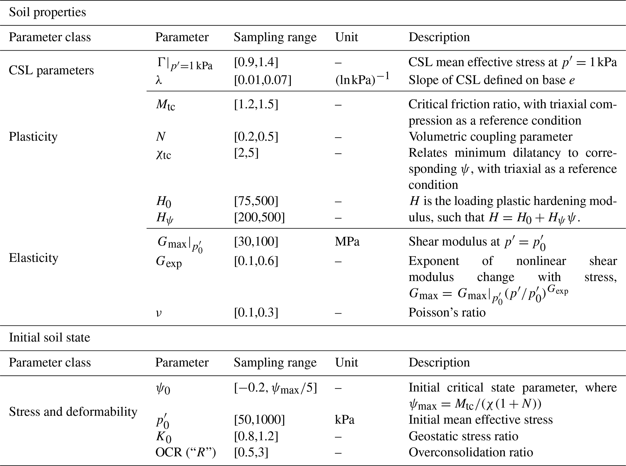
Table 1 Input values for NorSand model also used as inputs for the NorSandTXL VBA routine (Jefferies and Been, 2015).

3 NorSand

The NorSand constitutive model is a comprehensive critical state model that effectively accounts for the impact of void ratio on soil behavior, providing a robust framework for modeling static liquefaction in engineering applications. A distinctive characteristic of soils is that their void ratios or relative densities influence their mechanical properties. In this regard, NorSand, as a constitutive model, aptly elucidates changes in soil behavior resulting from variations in void ratio (Jefferies and Been, 2015).

Within the Critical State Soil Mechanics (CSSM) framework, NorSand aligns with widely used models like the Original Cam Clay (OCC; Schofield and Wroth, 1968) and the MCC (Roscoe and Burland, 1968). In fact, the NorSand and OCC yield surfaces have the same shapes and the same flow rules. CSSM is founded on two principles: (1) the presence of a unique failure locus known as the critical state locus (CSL) and (2) the assertion that shear strain guides soil toward the CSL.

The primary limitation of MCC, especially when applied to sands, lies in its inability to capture the dilation behavior observed in dense sands. Moreover, it proves inadequate in predicting the behavior of loose sands and is unsuitable for addressing liquefaction-related issues. NorSand's key advantage lies in its incorporation of a state parameter, representing the difference between the current void ratio of the soil and its critical state. This approach uniquely relates soil dilation or compaction to the state parameter (Rocscience, 2022).

NorSand stands out for its ease of use, particularly for practical geotechnical engineers. It relies on a minimal set of material properties, conveniently measurable through standard laboratory tests. The model effectively captures a wide range of soil behaviors influenced by varying density and confining stress. The key additional parameter, beyond what is necessary for defining an MCC model, is the state parameter. In situations where precision in representing volume change is crucial, the added effort required for parameter determination is more than justified.

Developed initially for sands based on observations in large-scale hydraulic fills such as tailing dams, NorSand applicability extends beyond, encompassing any soil where particle-to-particle interactions are controlled by contact forces and slips, rather than cohesive bonds. Present applications of NorSand span a range from well-graded tills to sands and clayey silts (Jefferies and Been, 2015).

The input parameters of the NorSand model are presented in Table 1, where the meaning of each parameter is also presented in the column “Description”. The sampling ranges presented will be discussed in the next section, as they are not intrinsic to the NorSand model.

4 Methods

4.1 Data generation

The NorSandTXL program is an Excel spreadsheet with all coding in the VBA environment and can be downloaded at http://www.crcpress.com/product/isbn/9781482213683 (last access: 8 February 2024), as indicated in the book by Jefferies and Been (2015). This particular spreadsheet simulates drained and undrained triaxial tests of materials governed by the NorSand constitutive model. The input features available in NorSandTXL are presented in Table 1, as well as their sampling ranges. The sampling ranges adopted come from literature results on the behavior of real granular materials. An initial version of such ranges was first presented by Jefferies and Shuttle (2002) and has been updated ever since. The ranges presented in Table 1 reflect the latest compilation available and reported by Jefferies and Been (2015). This way, practitioners will especially benefit from the datasets generated, since the parameters involved have been chosen so as to represent real granular materials.

In order to massively simulate triaxial test conditions for materials following the NorSand constitutive model, a Python routine has been developed. This routine performs two main steps: sampling and simulation. For the sampling process, all 14 input parameters are sampled in a nested manner, as there are two levels of hierarchy in the parameters: the higher level deals with the soil properties, which are unique for a given material, while the lower level considers the initial soil state during the triaxial tests. As a result, the sampling process needs to (a) account for different types of materials and (b) for each type of material, consider several testing conditions. Two datasets will be produced, as the next subsection will describe.

Thus, the following sampling procedure is considered to account for n_soils types of soils under n_conditions initial testing conditions:

• Sample the soil properties (the first 10 parameters in Table 1), obtaining a vector of properties sp_i, $i=\mathrm{1},\mathrm{\dots },n_{\mathrm{soils}}$, such that sp_i∈ℝ¹⁰. The sampling is performed using the centered Latin hypercube sampling (LHS) algorithm implemented in the Chaospy package (Feinberg and Langtangen, 2015) with a maximin criterion (first dataset) or using a Sobol (Sobol, 1967) quasi-Monte Carlo sampling technique implemented in SciPy (Virtanen et al., 2020) (second dataset).

• For each sp_i, the initial testing conditions (the last four parameters in Table 1) are sampled using the standard Latin hypercube sampling algorithm implemented in the Chaospy package (Feinberg and Langtangen, 2015) with a ratio criterion (first dataset) or a Halton (Halton, 1960) quasi-Monte Carlo sampling scheme (second dataset) implemented in SciPy (Virtanen et al., 2020). This way, the vectors $\mathit{i}{\mathit{c}}_{i,j}\in {\mathbb{R}}^{\mathrm{4}}$, $j=\mathrm{1},\mathrm{\dots },n_{\mathrm{conditions}}$ are obtained for each sp_i. The maximum value of ψ₀ is set to ${\mathit{\psi }}_{\max }/\mathrm{5}$ (as indicated in Table 1) for numerical stability. Additionally, to make the ic_i,j different for each sp_i, the random seed of the sampling algorithm is changed for each i.

From the procedure above, the matrix In of input parameters is obtained, whose rows are NorSandTXL input vectors obtained by concatenating each sp_i with all the ic_i,j, i.e., $$\begin{gathered} \left[\text{concat}\right(\mathit{s}{\mathit{p}}_{\mathrm{1}},\mathit{i}{\mathit{c}}_{\mathrm{1},\mathrm{1}}),\text{concat}(\mathit{s}{\mathit{p}}_{\mathrm{1}},\mathit{i}{\mathit{c}}_{\mathrm{1},\mathrm{2}}),\mathrm{\dots },\text{concat}(\mathit{s}{\mathit{p}}_{n_{\mathrm{soils}}}, \\ \mathit{i}{\mathit{c}}_{n_{\mathrm{soils}},n_{\mathrm{conditions}}}\left)\right] \end{gathered}$$, where “concat” denotes a concatenation operation between vectors. This implies that In is a (n_soilsn_conditions) by 14 matrix. The filling capabilities of the sampling schemes considered can be seen in Fig. 1.

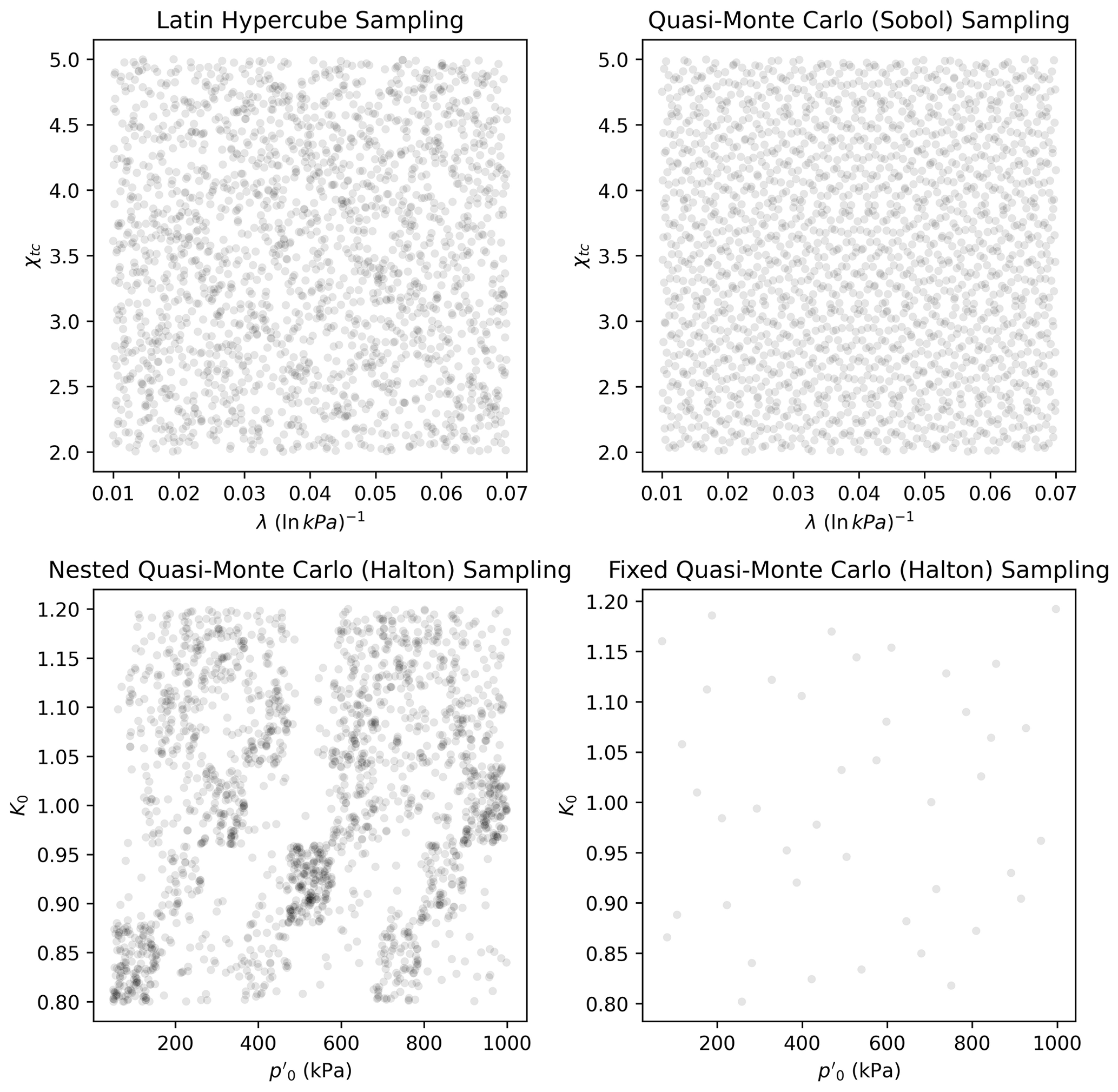
Figure 1 Scatter plot illustrating how each space-filling technique works for particular pairs of constitutive and test-related parameters.

Figure 1 reveals that the Latin hypercube sampling presents an apparent randomness on how the points are spread in the space. Quasi-Monte Carlo techniques, on the other hand, have a high predictability (as they are deterministic) but also fill in the input space adequately. The difference between the lower plots in Fig. 1 is that the lower-left plot presents the sampled pairs of values for a total of 2048 materials, while the lower-right plot presents the sampled pairs for a single material. The nested quasi-Monte Carlo sampling suffers from its deterministic nature, but shuffling the values helps to provide a better spread, as shall be discussed.

One may notice that besides ψ₀, which is restricted by a fraction of ψ_max, an independent sampling of input parameters was conducted. This was considered to explore the behavior of the NorSand model across all conceivable regions of the input parameter space. The objective was to enhance understanding of the analytical characteristics of the transfer function, which accepts these parameters as inputs and produces triaxial test results as outputs. This strategy ensures that the learning process remains unbiased, thereby preventing the algorithm from solely learning the transfer function within a specific area of interest. Broadening the scope of learning task beyond such confines can positively influence the overall learning process. For specific applications where the correlation among input parameters holds greater significance, adjusting loss weights for points within and outside the region of interest could be beneficial. This adjustment represents a choice that can be made. In future work, especially in the development of constitutive models tailored for specific purposes, it is advisable to consider this correlation structure.

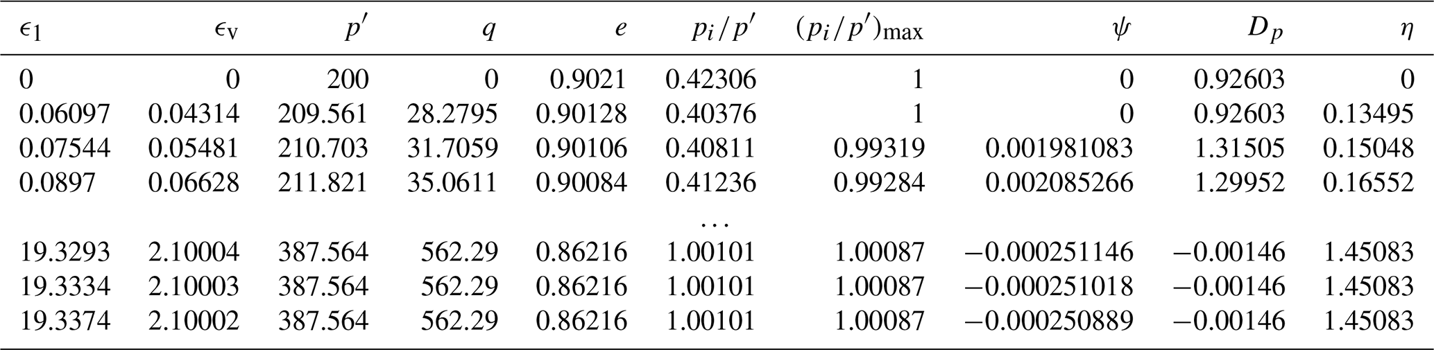
The simulation step involves opening the Excel spreadsheet provided in the book by Jefferies and Been (2015), inputting the sampled parameters, running both drained and undrained simulations for the input parameters and collecting their respective results. By design, the NorSandTXL Excel spreadsheet considers 4000 strain steps to go from zero to approximately 20 % nominal axial strain at the end of the simulated test. The authors of the spreadsheet indicate that this amount is both convenient and sufficient (Jefferies and Been, 2015). For a triaxial effective stress state with vertical stress ${\mathit{\sigma }}_a^{\prime }$ (kPa) and confining stress ${\mathit{\sigma }}_r^{\prime }$ (kPa), a total of 10 entities are reported from the tests, which are ϵ₁ (axial strain), ϵ_v (volumetric strain), $p^{\prime }=({\mathit{\sigma }}_a^{\prime }+\mathrm{2}{\mathit{\sigma }}_r^{\prime })/\mathrm{3}$ (mean effective stress in kPa), $q={\mathit{\sigma }}_a^{\prime }-{\mathit{\sigma }}_r^{\prime }$ (deviatoric stress in kPa), e (void ratio), $p_i/p^{\prime }$ (stress ratio), $(p_i/p^{\prime }{)}_{\max }$ (maximum stress ratio), ψ (state parameter), D_p (dilation) and $\mathit{\eta }=q/p^{\prime }$. Thus, the dataset is a 4000×10 array, as presented in Table 2.

Table 2 Example of the dataset collected from the NorSandTXL spreadsheet.

After the simulation is run, the results are saved in .h5 format files for postprocessing. The file extension .h5 is associated with the Hierarchical Data Format (HDF5) (The HDF Group, 1997-2023), which is a type of high-performance distributed file system. It is specifically designed to manage large and complex datasets efficiently and flexibly. Additionally, it enables a self-describing file format that is portable and supports parallel I/O for data compression (Lee et al., 2022), and has shown superior performance with high-dimensional and highly structured data (Nti-Addae et al., 2019). The literature indicates that the HDF5 has been popular in scientific communities since the late 1990s (Lee et al., 2022), which is evident by the large number of open-source and commercial software packages for data visualization and analysis that can read and write HDF5 (The HDF Group, 2023). As a result, this is the data format chosen for the present paper.

4.2 Sample size validation

The samples generated using the methods in the previous subsection need to be sufficiently large in order to represent the general behavior of the NorSand model. The best way to show that the sample size is sufficient is to study how a model calibrated (or trained) on a given dataset performs. So, we chose the most direct (and actually most important) learning task one could face while working with the datasets generated: back-calculation of the constitutive parameters of the model based solely on the triaxial test results. In short, from the triaxial tests we will learn the values of the parameters which govern the behavior of the material.

This way, it is possible to recall that a total of 14 parameters (10 constitutive and 4 related to test conditions) are used to generate the triaxial test results (4000×10 array where 4000 denotes the number of time steps of the loading process and 10 is the number of quantities monitored during the test), as presented in Table 2. From last subsection's notation, Let In_i (shape 1×14) be the ith row of the In matrix, which contains the constitutive parameters, and let ttu_i and ttd_i be the results of the triaxial test under undrained and drained conditions, respectively (4000×10 arrays, each) obtained by using these parameters on the NorSandTXL routine.

We will consider the following learning problem: from a sample of input parameters $\mathbf{In}={\text{In}}_{n,m}$, which considers n different types of soil and m different test configurations (therefore with nm rows), we will use the ttu_i (or ttd_i), for $i=\mathrm{1},\mathrm{\dots },nm$, to learn the vectors of parameters In_i, for $i=\mathrm{1},\mathrm{\dots },nm$. We wish to investigate what the values of n and m are that suffice to produce an accurate representation of the model. In order to do so, following standard learning tasks in a machine learning context, we need training, validation and testing data. It is worth noting that our methodology needs to be robust, so we indeed need the validation dataset because hyperparameter tuning will be performed.

The first dataset obtained by following the methods in Sect. 4.1 was generated by a Latin hypercube sampling (LHS) algorithm, which is known to provide low-discrepancy sequences of values (i.e., the samples are spread in the domain of the sampled variables). Despite being a really powerful technique, LHS lacks one relevant property: sequences obtained by LHS are not extensible. To put it simply, being extensible means that a sample of size j contains the values of the sample of size k, j>k. This way, it would not be possible to subsample from our original sample In in order to build smaller datasets without losing the space-filling capability of the dataset. This way, we needed to consider another sampling scheme to perform our investigation.

We chose to combine two quasi-Monte Carlo low discrepancy sequence generation techniques, i.e., Sobol (Sobol, 1967) and Halton (Halton, 1960), which are also extensible, to perform our tests. In that case, we generated a dataset with n=2048 and m=42 using Sobol sampling for the constitutive parameters (10 parameters) and Halton sampling for the experimental test condition variables (four variables) using the SciPy Python package (Virtanen et al., 2020). Both sequences have been scrambled (Owen and Rudolf, 2021) to improve their robustness for space filling. By using these parameters, we ran the NorSandTXL routine in the same manner as described in Sect. 4.1 and obtained the corresponding triaxial test results for both drained and undrained cases. Let us call this new dataset and qIn_2048,42.

By using the extensibility property of the sequences considered, 49 subsamples were taken: qIn_n,m for n in [32, 64, 128, 256, 512, 1024, 2048] and m in [6, 12, 18, 24, 30, 36, 42]. One may see that powers of 2 were used as sample sizes for the Sobol sampling scheme, which is standard and derives from its implementation in scipy.stats. It is worth noting that, in general, none of the entries of In_n,m will be in qIn_n,m, which indicates that using qIn_n,m for training and validation, and In_n,m for testing, does not allow for any data “leakage”. Besides, there is a clear benefit in using In_n,m as a test set: all the models will be tested on the same dataset.

For the learning task considered, we used the scikit-learn Python package (Pedregosa et al., 2011) and chose four algorithms: Ridge Regressor, KNeighbors Regressor and two variants of the Ridge Regressor which incorporate nonlinear mappings of the input and output values. The first two algorithms mentioned belong to two different classes: linear and neighbors-based regressors. They were chosen to illustrate how different types of algorithms learn our chosen task. The variants of the Ridge Regressor were chosen to account for nonlinearities by using the kernel trick. Considering the high dimensionality of the input datasets, using traditional kernels is not computationally feasible, so we used Nystroem kernels (Yang et al., 2012), which approximate a kernel map using a subset of the training data. By combining Nystroem kernels and Ridge Regressors, we can map the inputs to a nonlinear feature space and then consider a linear regression on these features. This is a similar approach to the one considered to build support vector machine regressors, but with a slightly different regularization for the decision boundary.

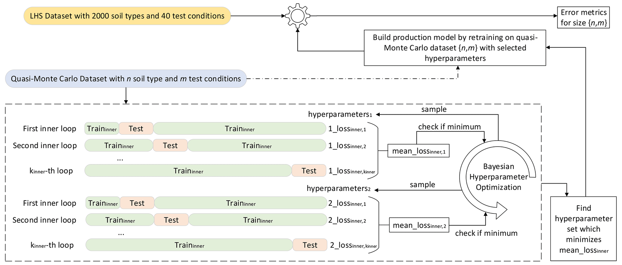
Figure 2 Methodology used to assess the sufficiency of the dataset containing 2000 soil types and 40 test conditions to represent the general behavior of the NorSand model.

We also considered mapping the output values (14 parameters, in our case) to the [0,1] range by combining the scikit-learn implementations of TransformedTargetRegressor and QuantileTransformer, which transforms the target values (outputs of the pipeline) to follow a uniform distribution. Therefore, for a given component, this transformation tends to spread out the most frequent values. It also reduces the impact of (marginal) outliers (Pedregosa et al., 2011). For all the algorithms considered, we also used a QuantileTransformer to preprocess the input values.

This way, Fig. 2 presents the methodology proposed and applied to assess the quality of the sample size. In the present paper, the LHS-generated dataset with n_soils=2000 and n_conditions=40, whose input parameter matrix is In_2000,40, will have its sufficiency assessed.

It is possible to describe the workflow in Fig. 2, for n in [32,64,128,256,512,1024,2048] and m in [6,12,18,24,30,36,42], as follows:

• For each simulated triaxial test corresponding to the parameter matrix qIn_n,m, select only the columns corresponding to ϵ₁, p^′, q and e (axial strain, mean effective stress, deviatoric stress and void ratio, respectively), which are the variables commonly measured and reported. The other seven columns are manipulations of these three (D_p or η, for example) and could be used as alternative regression variables, but such selection is not the focus of the present paper. This reduced simulation dataset is of shape 4000×4.

• Each triaxial test simulation may have different start/end values for ϵ₁, so it is important to “align” all the tests considered. By alignment we mean that all the tests will have measurements for the same values of ϵ₁. This will enable us to use this variable as an index and, therefore, decrease the dimensionality of each triaxial test simulation from 4000×4 to 4000×3. (Each line will correspond to a single value of ϵ₁.) We must select the smallest maximum value of ϵ₁ across all simulations (which was found to be around 15.74 % for the datasets considered and is represented as the vertical line in Figs. 3 and 4).

• Down-sample the 4000 time steps to 40 by using evenly spaced values on a logarithmic scale (function logspace from Python package NumPy): more values in the beginning of the time steps, where more changes are observed. This process is illustrated in Figs. 3 and 4, where the downsampling is performed for 40 points logarithmically spaced between ${\mathit{ϵ}}_{\mathrm{1}}={\mathrm{10}}^{-\mathrm{3}}\mathit{\%}$ and 15.78 %. This reduces each simulated triaxial test corresponding to the parameter matrix qIn_n,m from 4000×10 to 40×3. The concatenation of all triaxial test results corresponding to the parameter matrix qIn_n,m shall be named qInN_n,m and is of size $(nm,\mathrm{40},\mathrm{3})$.

• Perform a GroupKFold cross-validation scheme to find the best hyperparameters of an algorithm A using qInN_n,m as inputs and qIn_n,m as outputs. The loss function considered during the GroupKFold cross-validation is the mean absolute percentage error across all folds.

• Retrain the algorithm A using all qInN_n,m and qIn_n,m after fixing the hyperparameters as the optimal ones obtained during the cross-validation scheme.

• Test the trained algorithm A_t on ${\text{In}}_{n_h,m_h}$, where n_h and m_h are the hypothesized sufficient number of materials and test conditions, respectively.

• Obtain the mean absolute percentage error in the predictions of all the 14 input parameters corresponding to ${\text{In}}_{n_h,m_h}$.

• Get the overall mean error corresponding to all the input parameters.

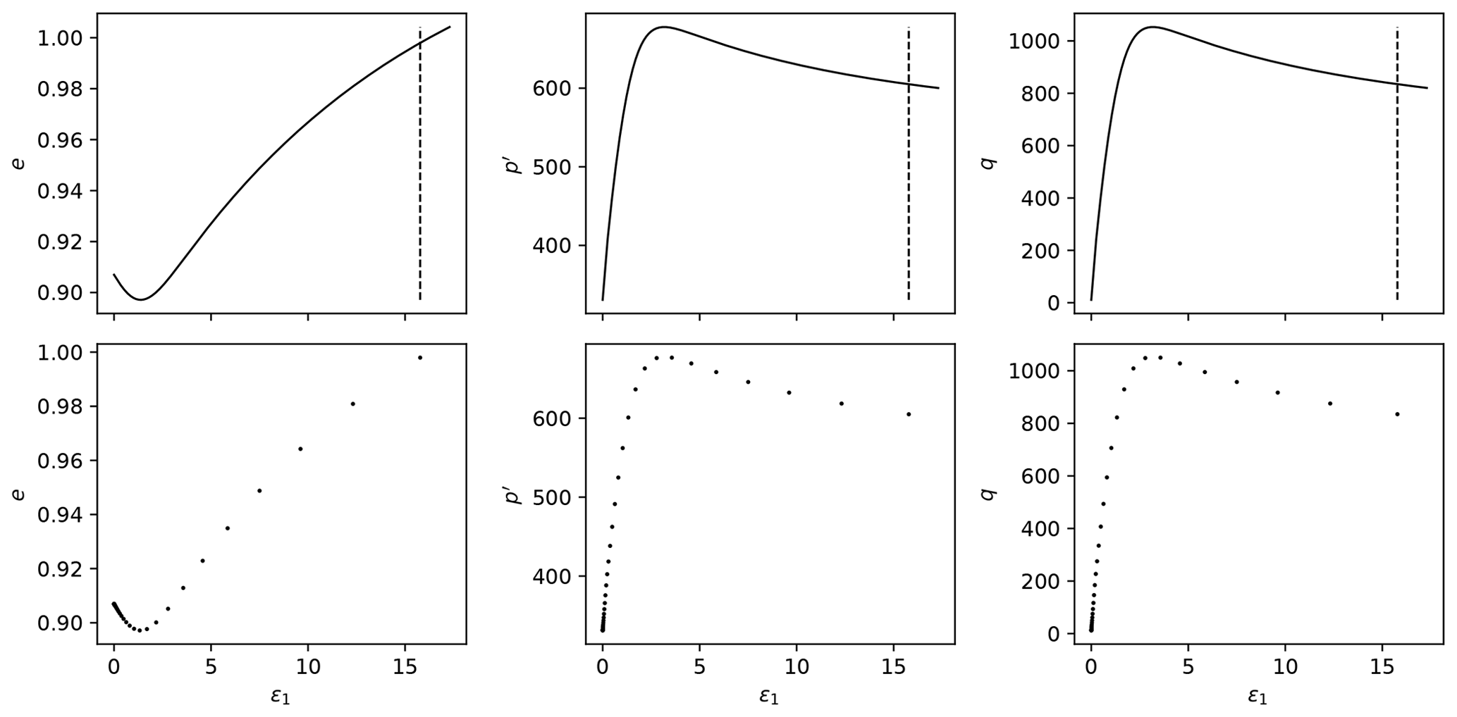
Figure 3 Downsampling process from 4000 to 40 points in the logarithmic scale for drained tests.

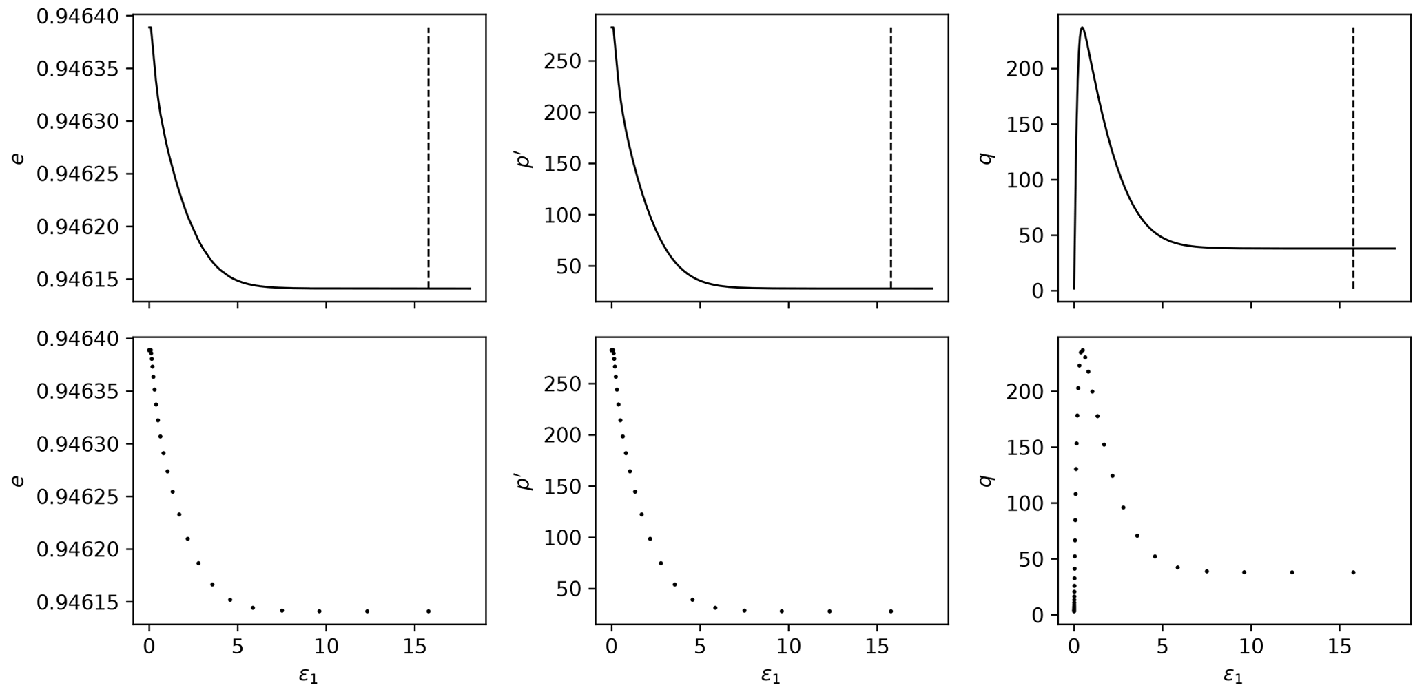
Figure 4 Downsampling process from 4000 to 40 points in the logarithmic scale for undrained tests.

As described, for training and validation, we considered a GroupKFold cross-validation technique, which is a K-fold iterator variant with non-overlapping groups (Pedregosa et al., 2011). This approach makes sure no material (group) is present in the training and validation sets, which would lead to data “leakage”.

A Bayesian optimization was performed to look for the best hyperparameters using the cross-validation folds generated. This process was carried out using the HyperOpt Python package (Bergstra et al., 2015), which considers tree-structured Parzen estimators. The search space for the Ridge and KNeighbors Regressors are the ones considered in the HyperOpt-Sklearn Python package (Komer et al., 2014). For the Nystroem kernel, a custom search space was defined and consisted of the following: “gamma” parameter uniformly on [0,1], “n_components” parameter as a random equi-probable choice among [600,1200,1800], “kernel” parameter as a random equi-probable choice among [“additive_chi2”, “chi2”, “cosine”, “linear”, “poly”, “polynomial”, “rbf”, “laplacian”, “sigmoid”], “degree” parameter as the integer value truncation of an uniform random variable on [1, 10] and “coef0” parameter uniformly on [0,1].

Finally, after the best hyperparameters are found, they are fixed and the algorithm A is retrained with the full dataset qInN_n,m. This calibrated version is then used to test the quality of the model on the triaxial test results corresponding to the dataset ${\text{In}}_{n_h,m_h}$. Then, the errors obtained for each model are plotted and analyzed. The reader can find the complete codes used to implement the steps above in Ozelim et al. (2023b).

5 Data records

In the present paper, it is shown that the LHS-generated dataset with n_soils=2000 and n_conditions=40 is a sufficient dataset. Thus, the folder containing such a dataset can be found in Ozelim et al. (2023a) and has the following structure:

NorSandTXL_H5 \ Simus\ TT\ Par_X_Y.h5

where TT stands for the test type (Drained or Undrained), X is the material index (from 0 to 1999) and Y is the sequential index for the input parameters (from 0 to 79999).

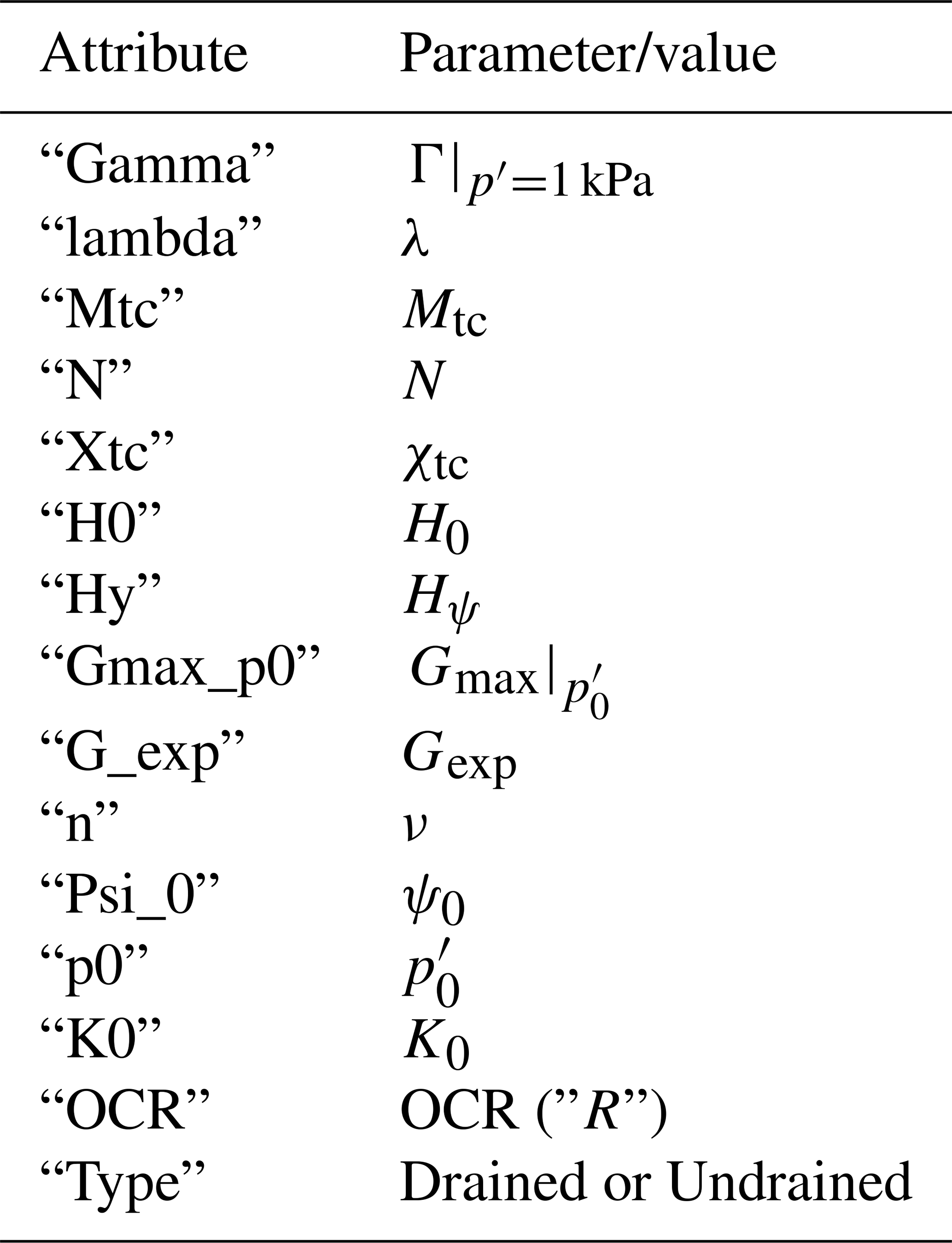
Each Par_X_Y.h5 file contains a dataset named NorSandTXL which includes the simulation results as presented in Table 2. It is worth noting that the values stored are of the type float32, which is sufficient for the applications envisioned for the dataset. In addition to the simulation results, the dataset also contains the attributes shown in Table 3. The correspondence between the attributes, whose data type is either float32 or <U7 (fixed-length character string of seven Unicode characters), and NorSandTXL input parameters is also presented in Table 3. It is easy to see that the dataset attributes in each file allow for a complete reproduction of the results, if desired. The units of the parameters are consistent with NorSandTXL, as presented in Table 1.

Table 3 Attributes of the NorSandTXL dataset present in each Par_X_Y.h5 file.

In order to prove the sufficiency of In_2000,40, we generated the dataset qIn_2048,42 following the methods previously presented. This latter dataset is also available in Ozelim et al. (2023a) with a similar folder structure. In that case, the upper-level folder is named NorSand_2048_42. It is worth noting that, due to upload difficulties, NorSand_2048_42 was split as NorSand_2048_42_Drained and NorSand_2048_42_Undrained, where each file contains the simulations for drained and undrained scenarios, respectively.

6 Technical validation

Considering that the engine running the triaxial test simulations is the Excel spreadsheet presented in the book by Jefferies and Been (2015) and that such a spreadsheet has been extensively validated by both academia and industry, there is no need to discuss the technical quality of the dataset. On the other hand, it is necessary to show that In_2000,40 suffices to cover the general behavior of the NorSand models.

By following the methods previously described and plotting the mean absolute percentage error (MAPE) result of the 49 models (each trained and validated with samples of different sizes subsampled from qIn_2048,42), Figs. 5 and 6 were obtained for drained and undrained conditions, respectively. The four algorithms considered were Ridge, KNeighbors, Ridge-K (with nonlinear kernel on inputs) and Ridge-KT (with nonlinear kernel on inputs and also QuantileTransformer on the outputs). It is clear in the figures that, for contours of 0.5 % gains in MAPE, the sample size of 2000×40 is actually more than enough for the learning task considered. This can be stated by noticing that the contours with lower error encompass samples with an exponential range of sizes. (The x axis is in log scale.) This indicates a really small gradient on the error in the n×m space, implying a good sample size. This happens for all four algorithms, indicating that not only linear and neighbors-based regressors have reached their maximum ability to learn, but also the nonlinear variants considered. It can be seen that the two nonlinear transformations applied (to inputs and to both inputs and outputs) present similar behavior, although with considerably smaller MAPEs.

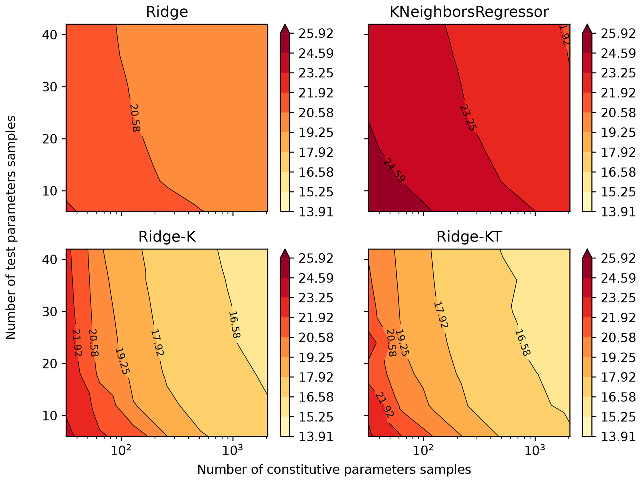
Figure 5 Mean absolute percentage error for all 14 parameters after being back-calculated solely from drained triaxial test results.

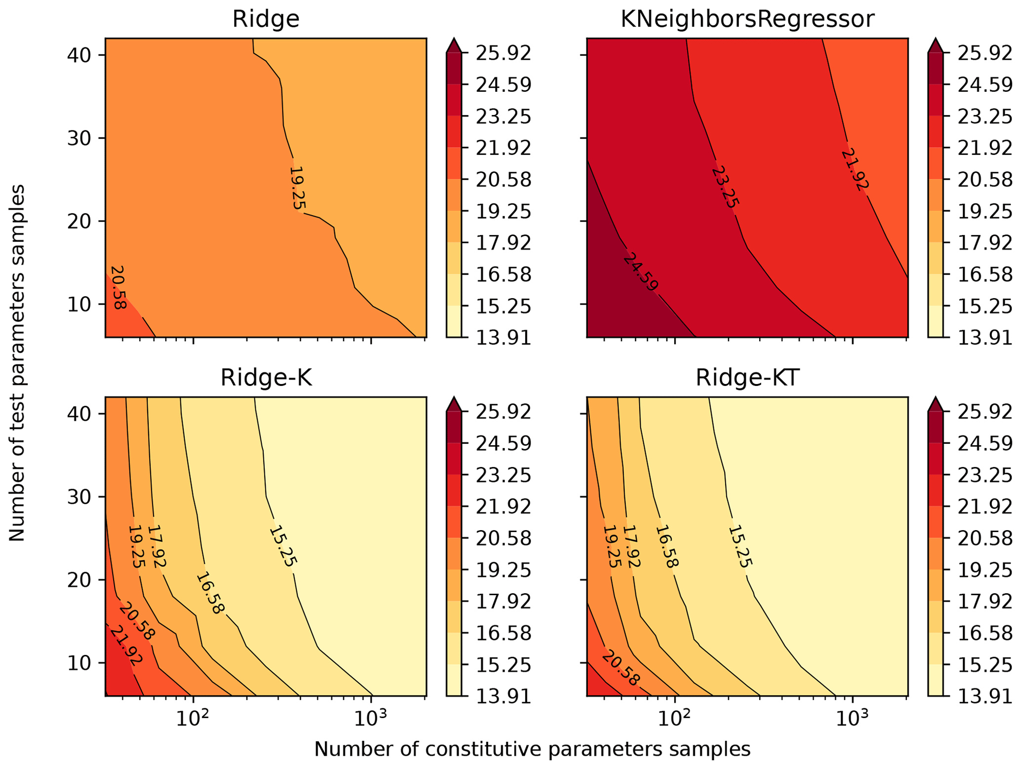
Figure 6 Mean absolute percentage error for all 14 parameters after being back-calculated solely from undrained triaxial test results.

Analysis of Figs. 5 and 6 indicates that for the learning task hereby considered, undrained tests generally presented a better performance when compared with drained tests. A possible cause for such behavior is that during undrained tests the void ratio is kept constant. Thus, for the learning task considered, the algorithm does not need to perform any nonlinear operations on one-third of the input dataset (which consists of e, p and q for 40 values of ϵ₁). So, with the same number of training samples and analytical structure of the learning algorithm, it is expected that fewer nonlinearities in the inputs would result in a better performance (smaller errors) of the predicted outputs.

Due to the space-filling qualities of both In_2000,40 and qIn_2048,42, qIn_2048,42 can also be considered a sufficient dataset to represent the NorSand model.

6.1 Understanding the learning task

6.1.1 Drained versus undrained test performance

Figure 7 presents the MAPE for each of the predicted parameters by the best performing algorithm (Ridge-KT trained and validated on the 2048×42 dataset and tested on the 2000×40 dataset).

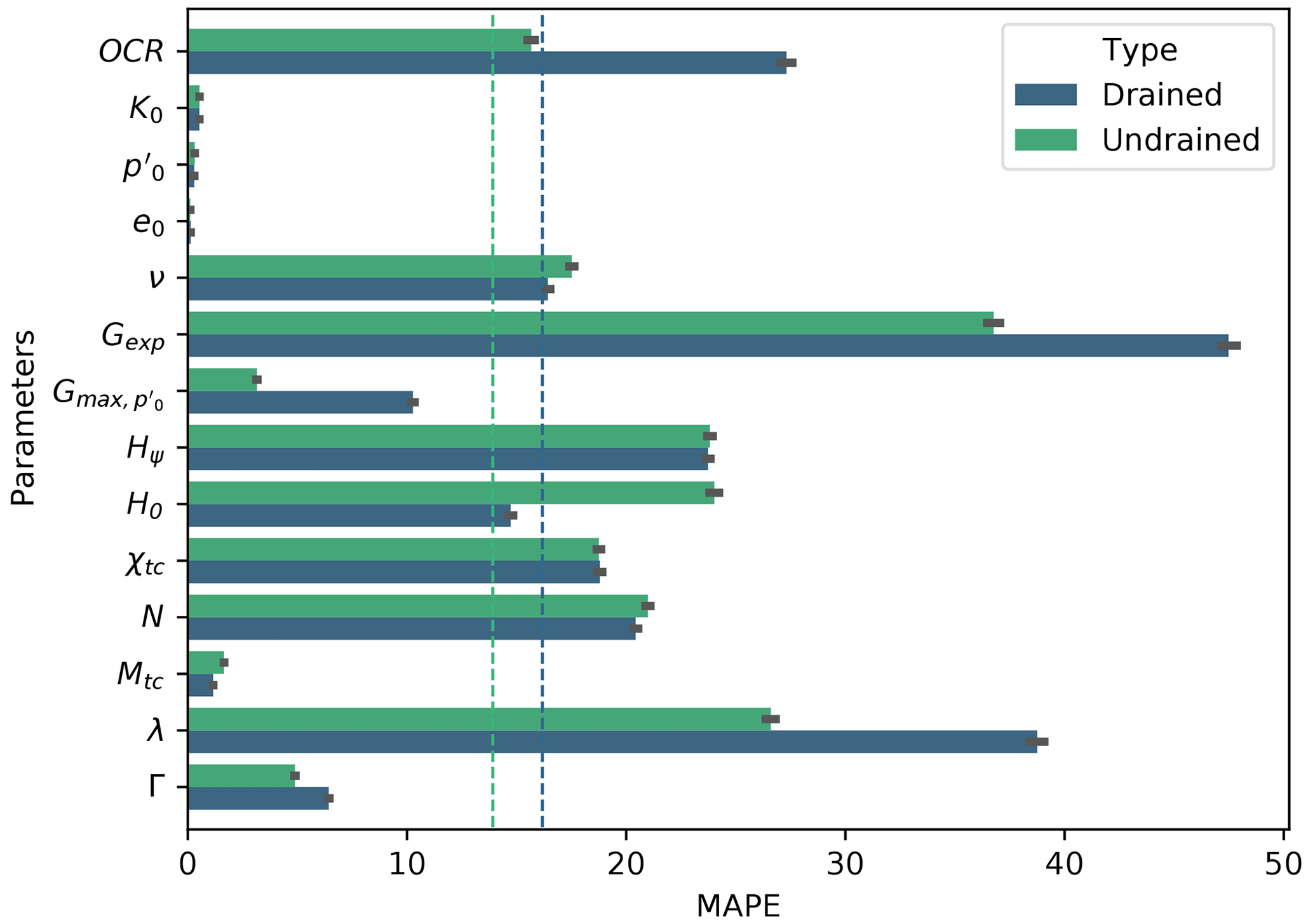
Figure 7 Drained and undrained mean absolute percentage errors for each parameter obtained by the best performing algorithm (Ridge-KT) with the 2048×42 training dataset. Vertical lines represent the mean MAPE for all parameters according to the colors in the plot (drained or undrained models).

At first glance, Fig. 7 suggests that using single tests to back-calculate parameters is not the best alternative, as the combination of both drained and undrained tests can potentially lead to better results. This will be the topic of future studies, especially on how many drained and undrained tests lead to optimal results. Jefferies and Been (2015) have discussed this situation, suggesting that the minimal combination would be of two undrained tests and one drained test.

Also from Fig. 7, it can be seen that, in general, the models trained on either drained or undrained datasets achieved a similar prediction performance for parameters K₀, $p_{\mathrm{0}}^{\prime }$, e₀, ν, H_ψ, χ_tc, N, M_tc and Γ. For the parameters linked to the test setup, namely K₀, $p_{\mathrm{0}}^{\prime }$ and e₀, this is somewhat expected as there are no nonlinearities involved in finding such values from triaxial test results. (It is a matter of simply checking the initial values of stresses and void ratios.)

For ν, what can be observed from Fig. 8 is that the ML algorithm did not fully succeed in its learning task, as there is a great spreading of the points along the identity line. In Fig. 8, most of the points are located in the central vertical region, indicating that most of the time, the predicted values were the closest to the midpoint of the interval (0.2), which is a naïve approximator known as a dummy regressor (which outputs the mean of the training dataset). This result may also be caused by the apparently low impact that ν has on the final result of the triaxial test.

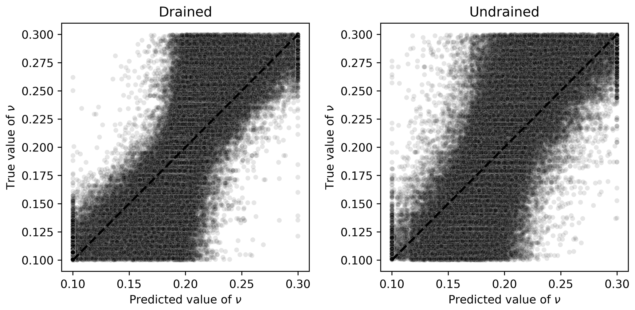
Figure 8 Scatter plots of true and predicted values for ν obtained by the best performing algorithm (Ridge-KT) with the 2048×42 training dataset for both drained and undrained tests.

The same dummy regressor behavior was observed for H_ψ, χ_tc, N and M_tc, as illustrated in Fig. 9. In this figure, it can be seen that the spreading of the points is still considerable around the identity line. Also, the most extreme mean-outputting behavior was observed for H_ψ, as Fig. 10 illustrates.

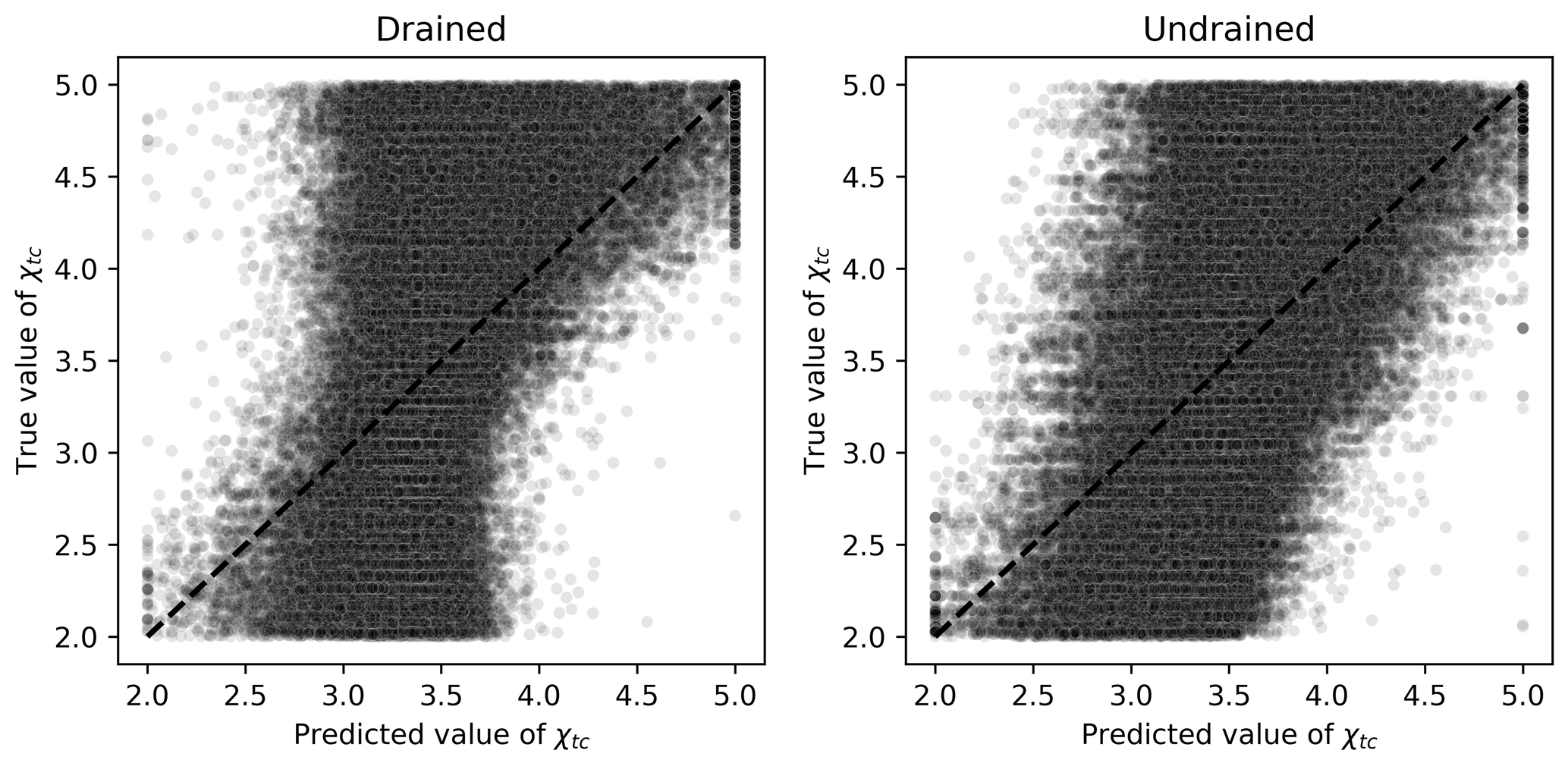
Figure 9 Scatter plots of true and predicted values for χ_tc obtained by the best performing algorithm (Ridge-KT) with the 2048×42 training dataset for both drained and undrained tests.

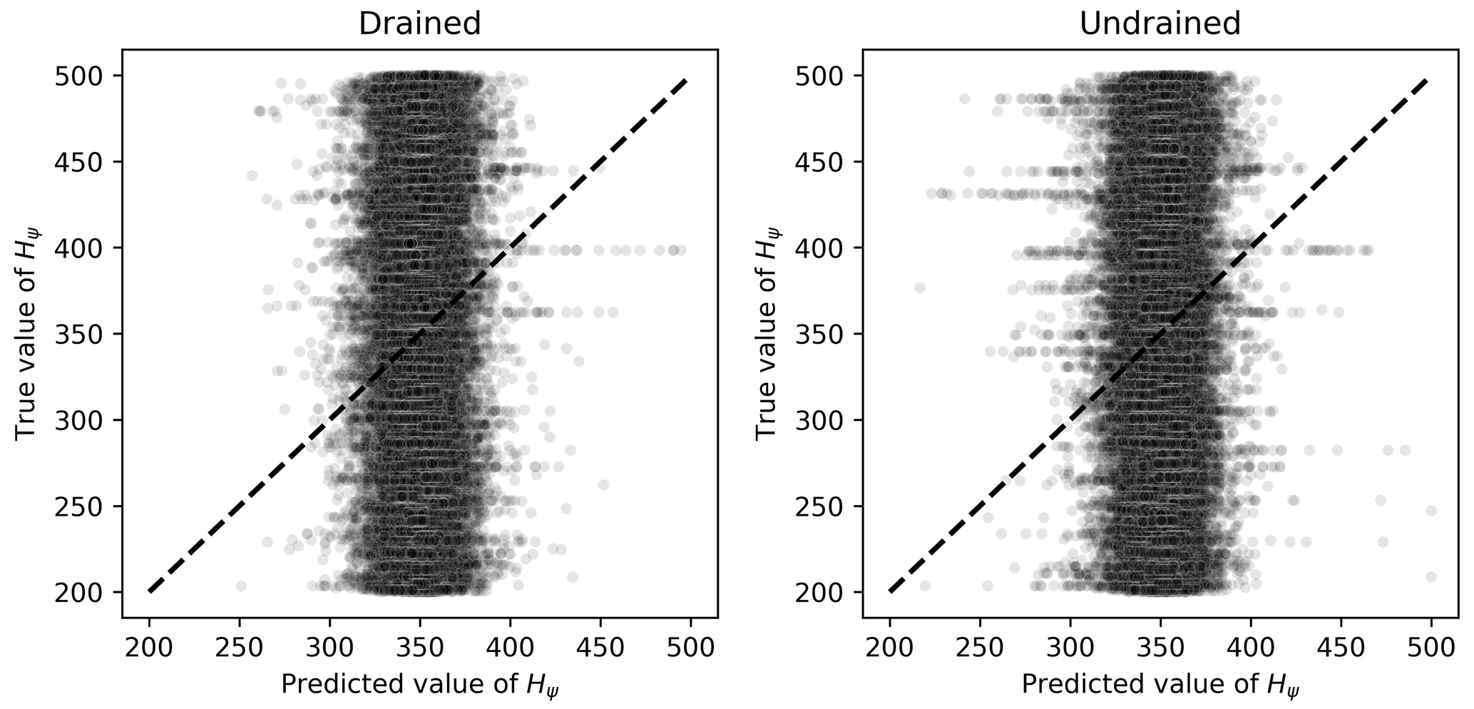
Figure 10 Scatter plots of true and predicted values for H_ψ obtained by the best performing algorithm (Ridge-KT) with the 2048×42 training dataset for both drained and undrained tests.

For Γ, Fig. 11 reveals that the mean-outputting behavior is not prominent anymore, revealing a good learning capability of the ML algorithm. Even though the MAPE is about the same for algorithms trained on either drained or undrained tests, for the undrained cases there is a more symmetric distribution of points around the identity line, which indicates less bias in the predictions. In this context, less bias and an equivalent MAPE would suggest that the ML algorithm trained on undrained tests is a better choice for estimating Γ.

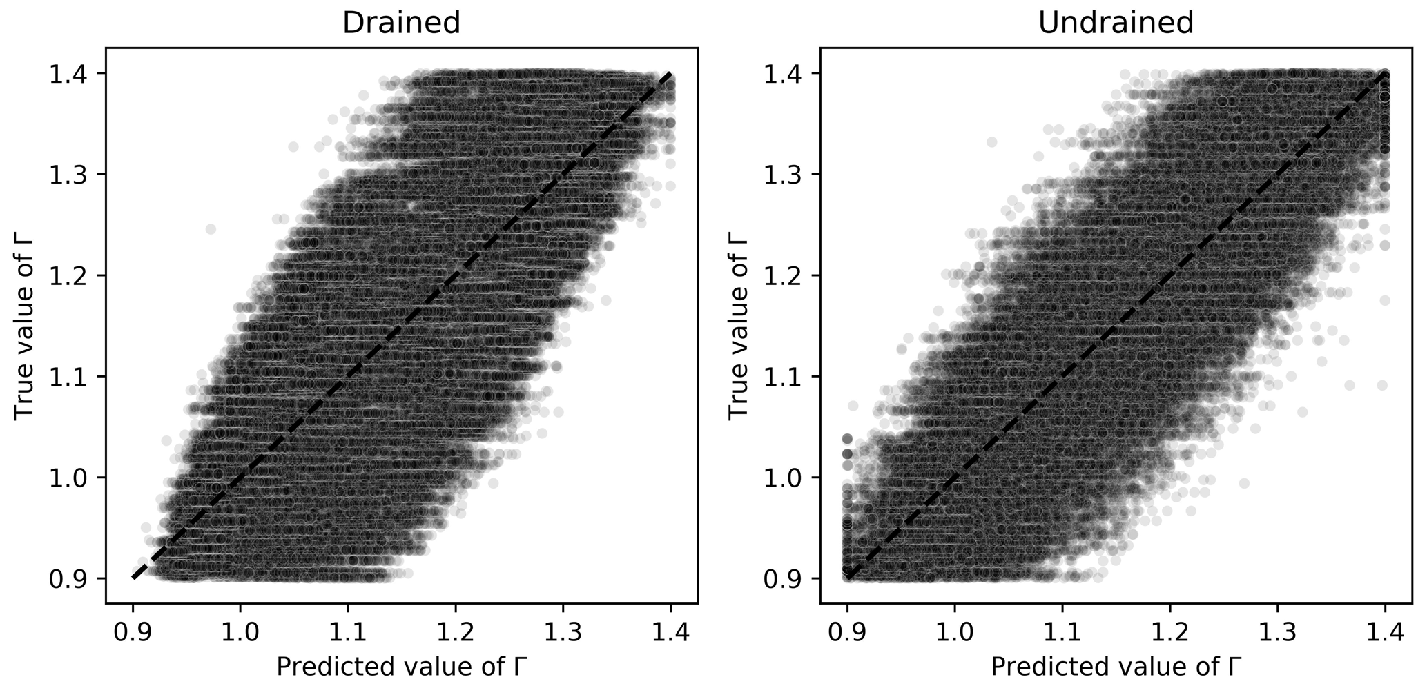
Figure 11 Scatter plots of true and predicted values for Γ obtained by the best performing algorithm (Ridge-KT) with the 2048×42 training dataset for both drained and undrained tests.

On the other hand, OCR, G_exp, $G_{\max ,p_{\mathrm{0}}^{\prime }}$ and λ had smaller MAPEs when predicted by algorithms trained on undrained tests. For the first three parameters, this is consistent with calibration procedures indicated in the literature (validation of elastic properties using undrained tests as suggested by Jefferies and Been, 2015). The performance of the Ridge-KT algorithm for these parameters can be seen in Figs. 12–14.

For the OCR values, it is clear from Fig. 12 that when drained tests are used to calibrate the ML algorithm, there is no clear trend in the plot. It is closer to a Z pattern, indicating a slight midpoint prediction behavior, which pulls the values closer to the mean training value. When undrained tests are used in the training and validation processes, there is a much clearer prediction pattern.

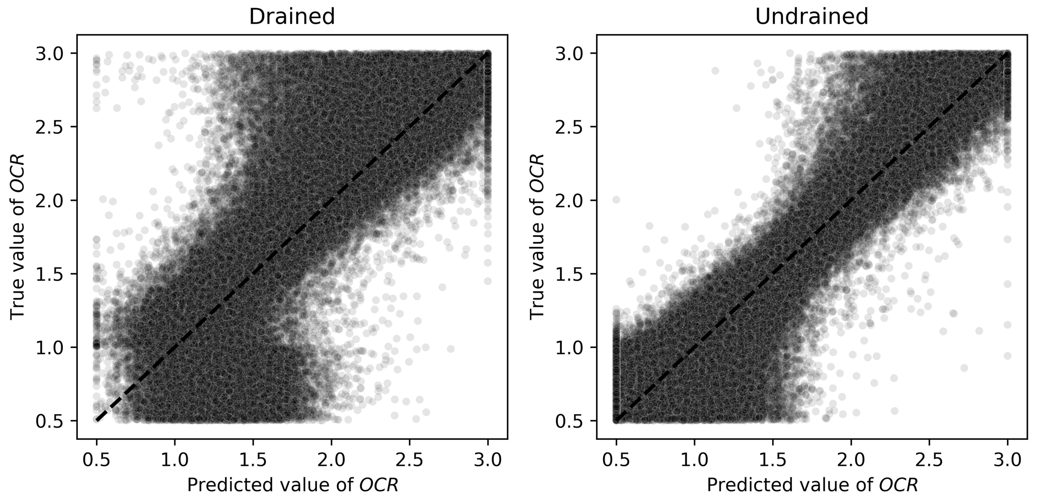
Figure 12 Scatter plots of true and predicted values for OCR obtained by the best performing algorithm (Ridge-KT) with the 2048×42 training dataset for both drained and undrained tests.

For the elastic properties G_exp and $G_{\max ,p_{\mathrm{0}}^{\prime }}$, Figs. 13 and 14 indicate clearly superior performances for algorithms trained and validated using undrained results. For G_exp, the relatively low impact of this parameter on the general outputs of the triaxial tests (within the range considered) could impair the learning tasks. A better performance is seen when undrained tests are used, but there is still room for improvement. This is not the case with $G_{\max ,p_{\mathrm{0}}^{\prime }}$, which has a clear sharp trend as seen in Fig. 14.

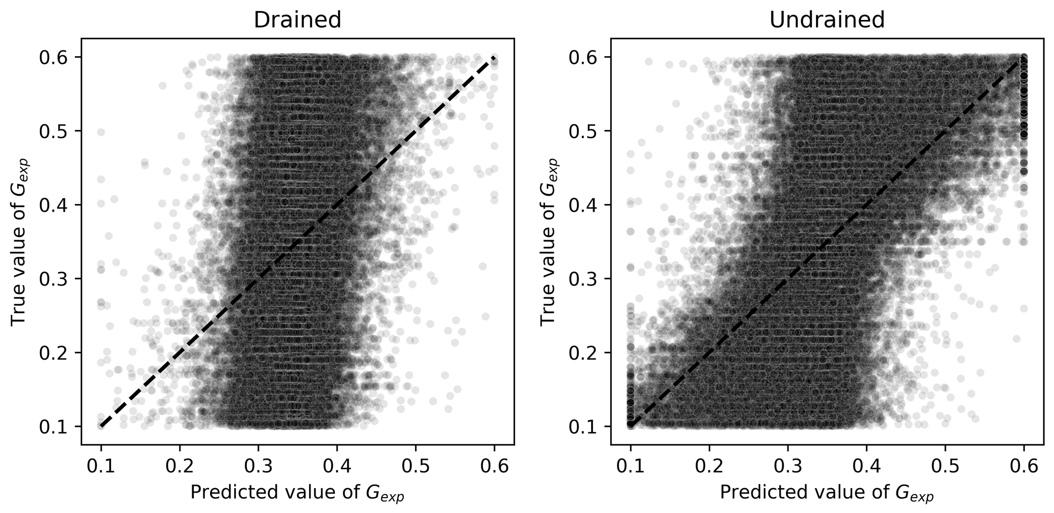
Figure 13 Scatter plots of true and predicted values for G_exp obtained by the best performing algorithm (Ridge-KT) with the 2048×42 training dataset for both drained and undrained tests.

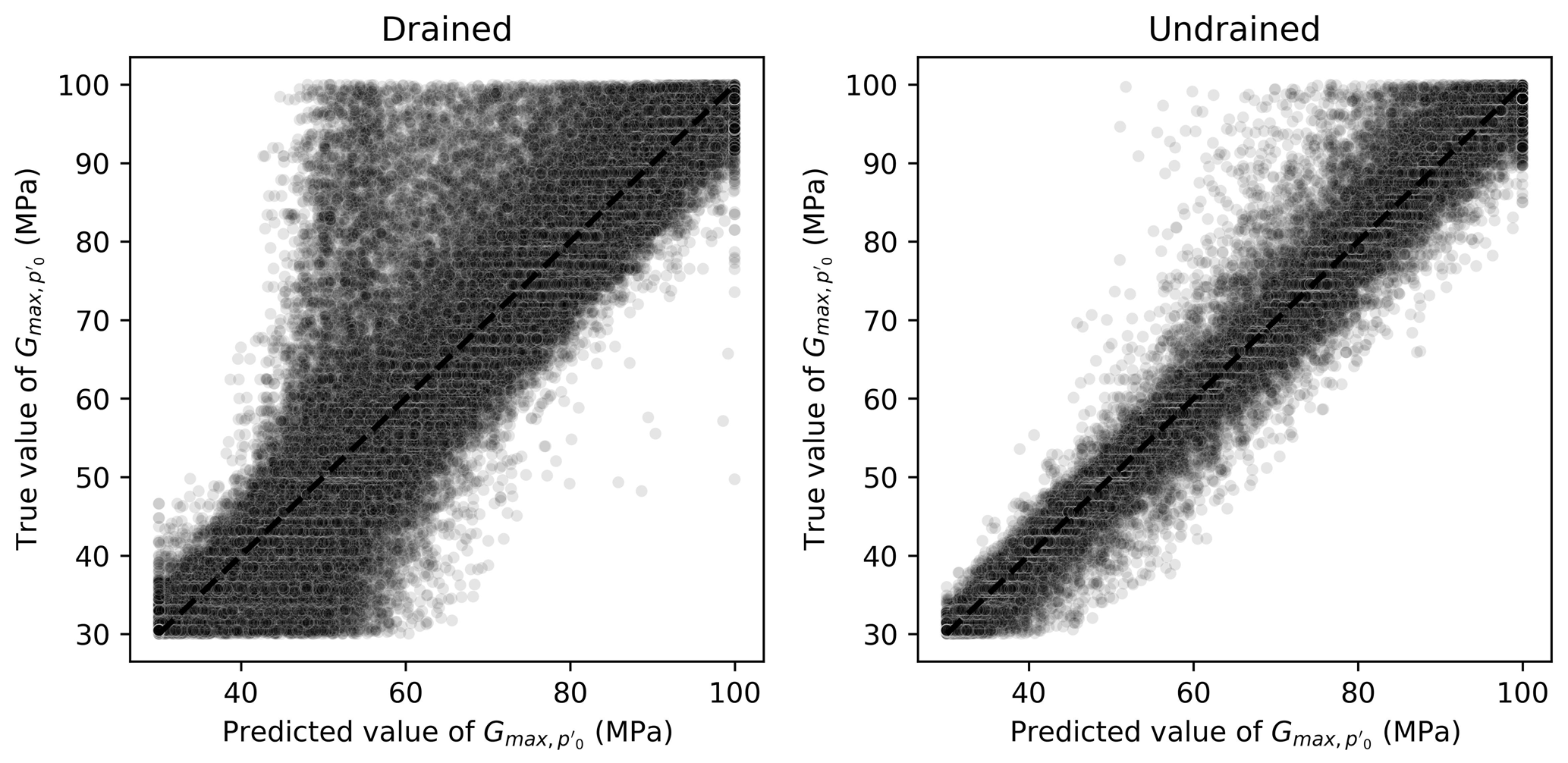
Figure 14 Scatter plots of true and predicted values for $G_{\max ,p_{\mathrm{0}}^{\prime }}$ obtained by the best performing algorithm (Ridge-KT) with the 2048×42 training dataset for both drained and undrained tests.

For λ, a similar behavior to Γ is observed regarding prediction biases, as seen in Fig. 15. The ML algorithm trained and validated using undrained tests provides a more balanced and symmetric prediction scenario, illustrating why it outperforms the algorithm calibrated using drained tests.

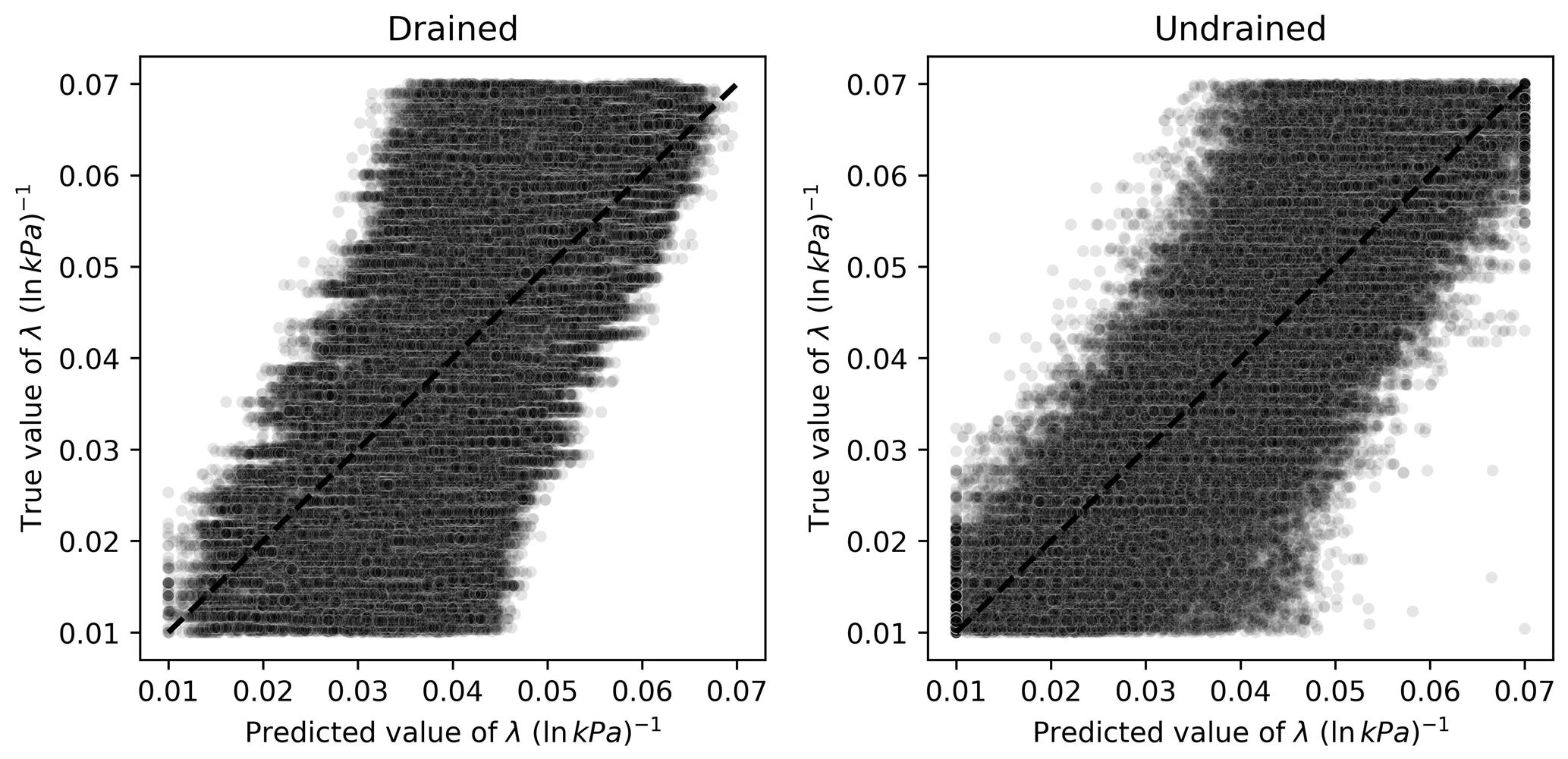
Figure 15 Scatter plots of true and predicted values for λ obtained by the best performing algorithm (Ridge-KT) with the 2048×42 training dataset for both drained and undrained tests.

The opposite situation arises for H₀, which is better predicted when drained tests are considered instead. This is also expected as these types of tests provide a better assessment of whether the stress and state–dilatancy properties inferred from the trends in the tests are self-consistent (Jefferies and Been, 2015). Figure 16 presents the results of both ML algorithms, indicating that a clearer trend is observed when drained tests are used as training and validation datasets. Even though there is also a trend when undrained tests are used, the spread around the identity line is considerable, increasing the MAPE value.

Figure 16 Scatter plots of true and predicted values for H₀ obtained by the best performing algorithm (Ridge-KT) with the 2048×42 training dataset for both drained and undrained tests.

6.1.2 Effect of training sample sizes on the learning task

In analyzing Figs. 5 and 6, apparently the overall MAPE slightly increases in the bottom-right corner (large constitutive parameter samples with lower test parameter samples). This is a visual artifice caused by the application of the log scale to the horizontal axis, which ends up compressing the values on that corner. If the natural scale were considered, one would see that the opposite occurs: large constitutive parameter samples with lower test parameter samples give better results when compared with small constitutive parameter samples with large test parameter samples. Such behavior can be explained by the fact that of the 14 parameters, 10 correspond to constitutive parameters, so fewer training samples impair their learning task.

A MAPE comparison is presented in Figs. 17 and 18 for both drained and undrained tests with different training samples' diversities. (We compare the best performing models obtained by the Ridge-KT algorithm, which uses the 2048×42 dataset, to two other cases: 32×42 and 2048×6 training samples.) It is possible to see that the errors of the 10 constitutive parameters exhibit greater sensitivity to fewer training samples than the opposite situation with test parameters. Except for OCR, all the other heavily impaired parameters are constitutive.

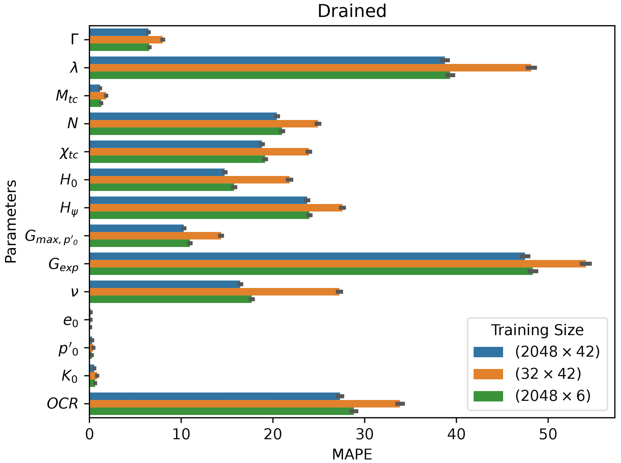
Figure 17 Drained mean absolute percentage errors obtained for each parameter by the best performing algorithm (Ridge-KT) with training datasets of different size.

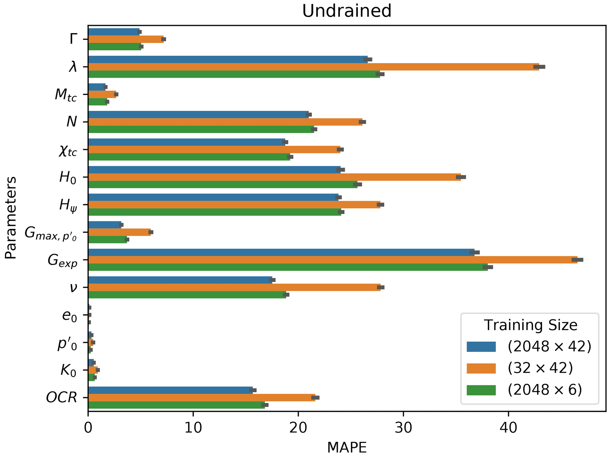
Figure 18 Undrained mean absolute percentage errors obtained for each parameter by the best performing algorithm (Ridge-KT) with training datasets of different size.

7 Usage notes and codes

In Python, the h5py package provides all the necessary tools to interact with the .h5 files produced and made available in the NorSand4AI dataset. Depending on the intended application, it might be beneficial to down-sample the 4000×10 matrix to increase the axial strain increments. This can be accomplished using standard Python packages such as pandas and NumPy. In this section, the codes used to generate the datasets are presented. At first, the Python packages indicated in Listing 1 need to be imported.

Listing 1 Python packages needed.

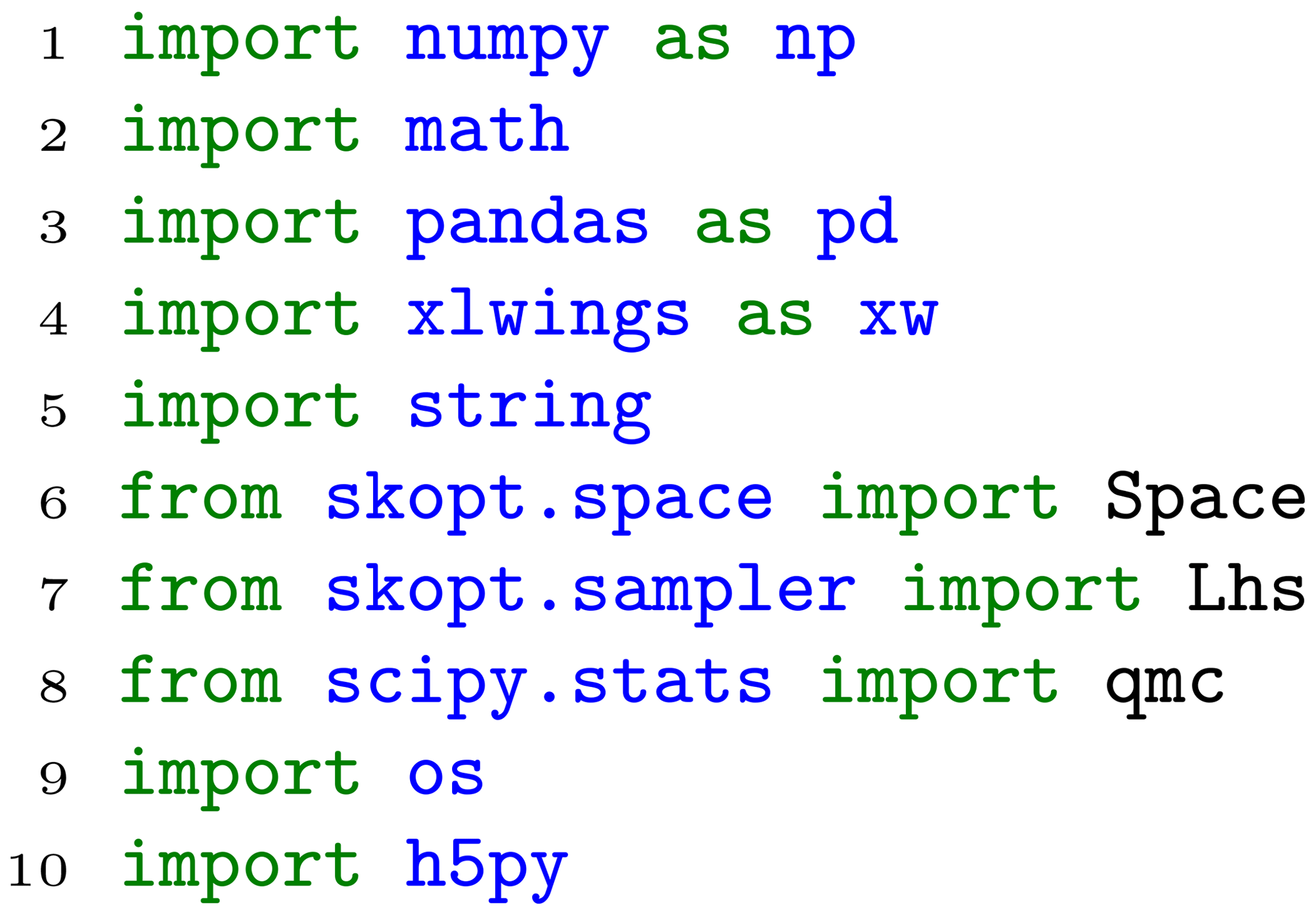
The packages NumPy, math and pandas are required for data manipulation and numeric calculations. The xlwings package is needed to bridge Python and Excel. Furthermore, the string package is necessary to convert the (row–column) positional encoding to the (row–letter) alphanumeric encoding used in Excel. For the Latin hypercube sampling procedure, skopt is required, while qmc from scipy.stats is needed for the quasi-Monte Carlo sampling. Lastly, for creating folders and files, both os and h5py should be imported.

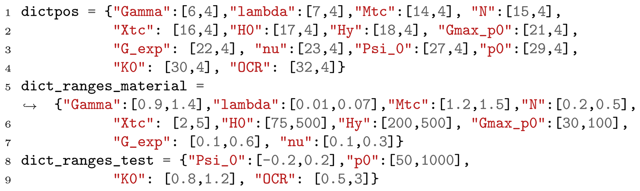
Let dictpos be a dictionary that points to the locations in the spreadsheet of the cells corresponding to each input parameter. Additionally, let dict_ranges_material and dict_ranges_test be dictionaries specifying the sampling ranges of the input parameters. For this paper, these dictionaries are presented in Listing 2.

Listing 2 Definition of auxiliary dictionaries.

Listing 3 The run_NorSand function.

7.1 Simply run NorSand in Python

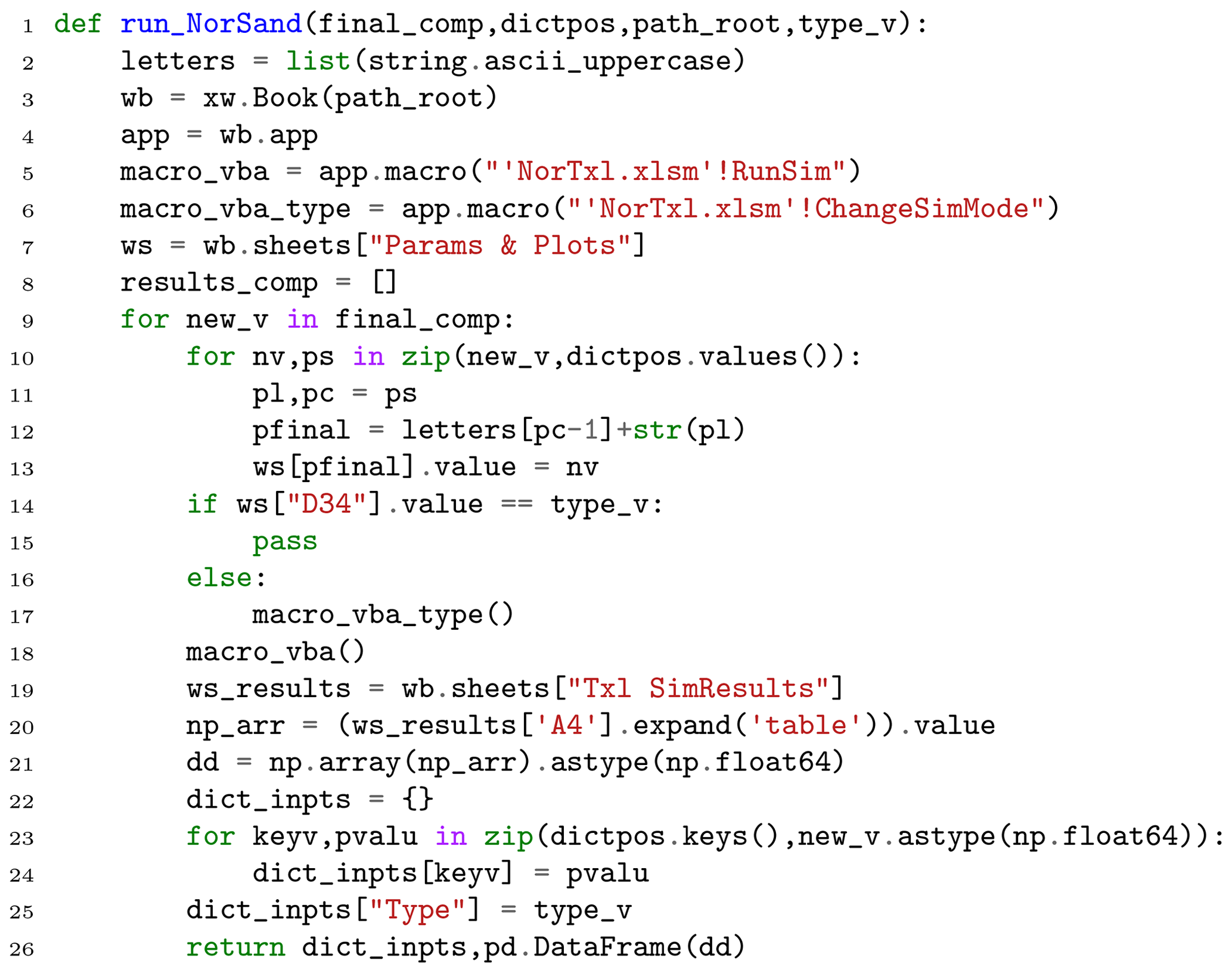
If one seeks to simply run NorSand in Python, the function run_NorSand presented in Listing 3 can be used. Its inputs are

• final_comp: input parameters as a NumPy array of shape (1,14). The parameters need to be inserted in the same order as dictpos.keys(), i.e., [“Gamma”, “lambda”, “Mtc”, “N”, “Xtc”, “H0”, “Hy”, “Gmax_p0”, “G_exp”, “nu”, “Psi_0”, “p0”, “K0”, “OCR”];

• dictpos: dictionary to locate the parameters inside the spreadsheet;

• path_root: path of the spreadsheet “NorTxl.xlsm”, obtained at http://www.crcpress.com/product/isbn/9781482213683 (last access: 8 February 2024);

• type_v: type of the simulation (either “Drained” or “Undrained”).

This function outputs two entities: a dictionary containing the parameters inserted to run the simulation and a 4000×10 pandas dataframe with simulation results (which are located within the “Txl SimResults” tab of the xlsm file). The columns are the ones presented in Table 3.

7.2 Generate and save files

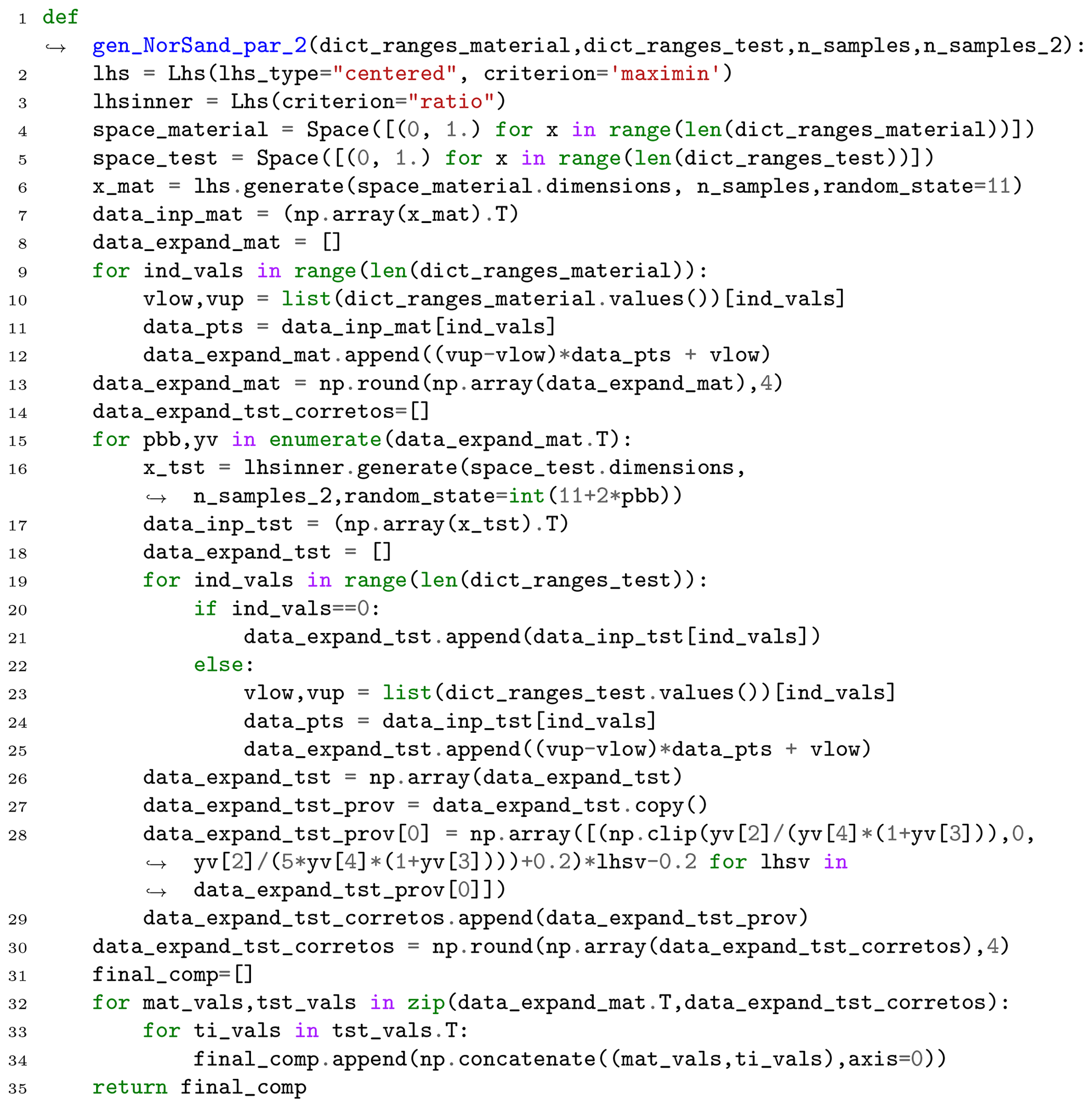
To generate the LHS inputs for the NorSandTXL spreadsheet, considering n_samples soil types and n_samples_2 initial test conditions, the function gen_NorSand_par_2, presented in Listing 4, was considered.

Listing 4 The gen_NorSand_par_2 function.

The quasi-Monte Carlo sampling schemes (Sobol and Halton) can be used to generate the input samples by means of the gen_NorSand_par_LD function, presented in Listing 5.

Listing 5 The gen_NorSand_par_LD function.

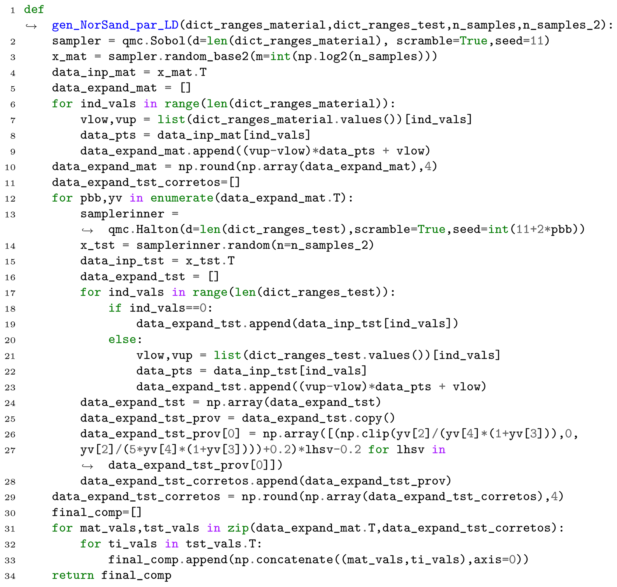
Furthermore, to run the NorSandTXL Excel spreadsheet located in path_xlsm for all the input parameters previously obtained as final_comp = gen_NorSand_par_2 (dict_ranges_material, dict_ranges_test,n_samples,n_samples_2) (or final_comp = gen_NorSand_par_LD(dict_ranges_material, dict_ranges_test,n_samples,n_samples_2) for the quasi-Monte Carlo sampling of inputs), the function run_NorSand_simus_P can be run. This function is presented in Listing 6.

Listing 6 The run_NorSand_simus_P function.

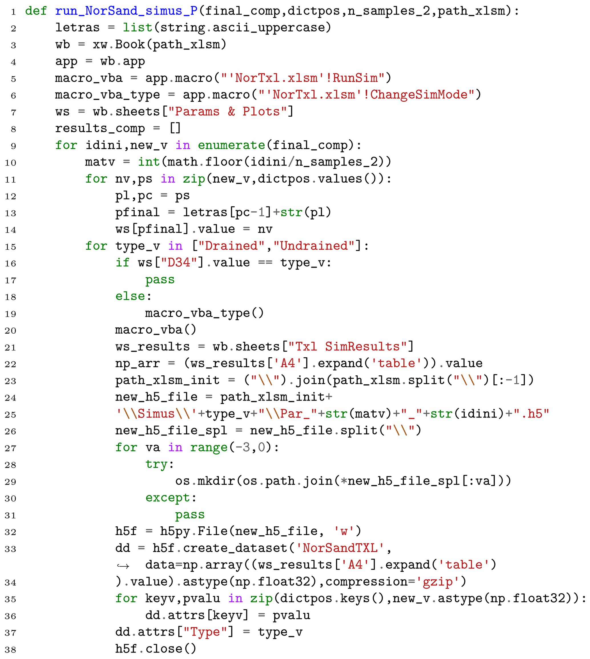
The function run_NorSand_simus_P runs the simulation and also saves the results as .h5 files in the same folder as the Excel spreadsheet. In this case, the new files are saved following the naming convention and folder structure discussed in the paper.

It is worth noting that for the LHS sampling with 2000 soil types and 40 test conditions, two values of sampled ψ₀ needed to be reduced due to instabilities in the VBA code calculations. These values were

• final_comp[19572][10]=0.085 and

• final_comp[10929][10]=0.082.

Furthermore, for the quasi-Monte Carlo sampling with 2048 soil types and 42 test conditions, five values of sampled ψ₀ needed to be reduced due to the same reasons. These values were

• final_comp[56382][10]=0.0849,

• final_comp[57476][10]=0.0766,

• final_comp[85371][10]=0.0955,

• final_comp[34971][10]=0.08 and

• final_comp[41245][10]=0.072.

All the codes previously presented are available as the Jupyter notebook Sample_and_Run.ipynb in Ozelim et al. (2023b).

7.3 Analyzing errors during learning tasks

As described in the Methods section, we perform a sample size validation. Considering that the codes for such validation are lengthy, they are presented in Ozelim et al. (2023b). The Jupyter notebook Sample_size_validation.ipynb is fully commented to illustrate its usage.

8 Conclusions

Obtaining massive datasets for modeling the behavior of soils is of great interest, not only because new artificial intelligence algorithms can be built, but also to assess the adequacy of newly proposed physically informed models. In the context of critical state approaches, the NorSand model has been shown to provide a good balance between complexity and accuracy. Also, this model is used to assess the liquefaction potential of soils, which is a major cause of high scale disasters lately, such as tailing dams' failures.

In this study, major issues were addressed. Firstly, the paper tackled the challenges associated with the quantity and complexity of synthetic datasets required for nonlinear constitutive modeling of soils. This was achieved by simulating both drained and undrained triaxial tests, resulting in two datasets. The first dataset involved a nested Latin hypercube sampling of input parameters, covering 2000 soil types with 40 initial test configurations for each, yielding a total of 160 000 triaxial test results. The second dataset employed a nested quasi-Monte Carlo sampling (Sobol and Halton) of input parameters, encompassing 2048 soil types with 42 initial test configurations for each, resulting in a total of 172 032 triaxial test results. Each simulation dataset was represented as a matrix of dimensions 4000×10. The study demonstrated that the dataset of 2000 soil types and 40 initial test configurations adequately captured the general behavior of the NorSand model.

Secondly, the paper addressed the issue of the availability of open-source implementations of the NorSand constitutive model. This was achieved by presenting an implementation that connects the well-established VBA implementation to the Python environment. The VBA code served as the “processing kernel” for the new Python implementation, leveraging the extensive testing and validation conducted by Jefferies and Been (2015). This integration allows researchers to harness the full capabilities of Python packages in their analyses involving the NorSand model.

A comprehensive database like the one provided is crucial for developing ML and artificial intelligence models of geotechnical materials. In particular, all geotechnical critical state models involve specific simplifications, with the most apparent being their reliance on “remolded” or disturbed soil properties. Understanding the consequences of such structural alterations, especially in terms of their impact on the apparent OCR, poses notable challenges. The effect on the stress ratio (ψ) remains unclear. Through the utilization of physics-informed machine learning and artificial intelligence algorithms, these uncertainties can be thoroughly investigated, uncovering patterns and hidden features within experimental data. We are confident that the results of the present paper are useful assets in this quest, being useful for both academic and industrial communities. Furthermore, researchers interested in modeling sequential data, such as time series, could use this dataset for benchmarking purposes, as the highly nonlinear nature of the constitutive model poses a significant challenge to ML and DL techniques.