the Creative Commons Attribution 4.0 License.
the Creative Commons Attribution 4.0 License.
 | 10 Apr 2024
Decision Support System version 1.0 (DSS v1.0) for air quality management in Delhi, India
Gaurav Govardhan
Sachin D. Ghude
Rajesh Kumar
Sumit Sharma
Preeti Gunwani
Chinmay Jena
Prafull Yadav
Shubhangi Ingle
Sreyashi Debnath
Pooja Pawar
Prodip Acharja
Rajmal Jat
Gayatry Kalita
Rupal Ambulkar
Santosh Kulkarni
Akshara Kaginalkar
Vijay K. Soni
Ravi S. Nanjundiah
Madhavan Rajeevan
This paper discusses the newly developed Decision Support System version 1.0 (DSS v1.0) for air quality management activities in Delhi, India. In addition to standard air quality forecasts, DSS provides the contribution of Delhi, its surrounding districts, and stubble-burning fires in the neighboring states of Punjab and Haryana to the PM2.5 load in Delhi. DSS also quantifies the effects of local and neighborhood emission-source-level interventions on the pollution load in Delhi. The DSS-simulated Air Quality Index for the post-monsoon and winter seasons of 2021–2022 shows high accuracy (up to 80 %) and a very low false alarm ratio (∼ 20 %) from day 1 to day 5 of the forecasts, especially when the ambient air quality index (AQI) is > 300. During the post-monsoon season (winter season), emissions from Delhi, the rest of the National Capital Region (NCR)'s districts, biomass-burning activities, and all other remaining regions on average contribute 34.4 % (33.4 %), 31 % (40.2 %), 7.3 % (0.1 %), and 27.3 % (26.4 %), respectively, to the PM2.5 load in Delhi. During peak pollution events (stubble-burning periods or wintertime), however, the contribution from the main sources (farm fires in Punjab–Haryana or local sources within Delhi) could reach 65 %–69 %. According to DSS, a 20 % (40 %) reduction in anthropogenic emissions across all NCR districts would result in a 12 % (24 %) reduction in PM2.5 in Delhi on a seasonal mean basis. DSS is a critical tool for policymakers because it provides such information daily through a single simulation with a plethora of emission reduction scenarios.
- Article
(4340 KB) - Full-text XML
-
Supplement
(805 KB) - BibTeX
- EndNote


The national capital of India, Delhi, is one of the most populated capitals in the world, with an estimated count of more than 18.7 million (Census Of India 2011, 2020). Immense population density, urbanization, and industrialization within the city have resulted in many urban issues, including air pollution (Molina and Molina, 2004; Chopra, 2016; Zhang et al., 2022). The primary sources of pollutants are vehicles, industries, power plants, waste-burning practices, construction and demolition activities, and road dust. On top of this, the post-monsoonal (October–November) harvesting of the paddy crops and the associated burning of the paddy residue in the neighboring states of Haryana and Punjab also contribute to the degradation of air quality in Delhi and the surrounding region (Bikkina et al., 2019; Bray et al., 2019; Chowdhury et al., 2019; Kulkarni et al., 2020; Nair et al., 2020). Besides, the geographical location and the local meteorological conditions, especially during the winter months, aggravate the pollution levels in the city (Guttikunda and Gurjar, 2012; Tiwari et al., 2014; Kumar et al., 2020. The pollution in the city is at its peak during the post-monsoon and the winter seasons, though the summer (April–June) months also bring severe dust storms and the associated degradation of Delhi's air quality (Banerjee et al., 2021; Chakravarty et al., 2021; Parde et al., 2022). The air quality in Delhi is so poor that it occasionally (especially during the post-monsoon and winter seasons) crosses the national air quality standards by more than 10 times (Kanawade et al., 2020; Jena et al., 2021; Roozitalab et al., 2021). Owing to the ever-increasing pollution, Delhi has been topping the list of the most polluted national capital cities in the world (Meteosim, 2019). It has been estimated that the air pollution in Delhi is causing more than 7000 premature mortalities every year (Guttikunda and Goel, 2013; Ghude et al., 2016; Saini and Sharma, 2020). The loss of average life expectancy in the city is also estimated to be around 2 years in Delhi (Ghude et al., 2016; Guo et al., 2018).
The primary solution to this problem lies in the reduction in the anthropogenic emissions happening in and around the city. However, permanent mitigation of emissions is a long-term objective due to the involvement of multiple socioeconomic factors (Riahi et al., 2017). A short-term and effective solution to this problem could be related to creating awareness in the public about air pollution, releasing early warnings about the air pollution episodes that are likely to happen, and imposing temporary emission controls so that the exposure of the common people to acute levels of air pollution could be avoided. With this motivation, the Government of India, in the year 2018, directed the Ministry of Earth Sciences (MoES) to develop an early-warning system for air pollution events happening in Delhi. With this mandate, the Indian Institute of Tropical Meteorology (IITM), Pune, and the India Meteorological Department (IMD) developed the Air Quality Early Warning System (AQEWS) in collaboration with the National Center for Atmospheric Research (NCAR), USA, in 2018. AQEWS is a dynamical modeling system that simulates air quality over the entire India with a special focus on Delhi (Ghude et al., 2020; Kumar et al., 2020; Jena et al., 2021; Sengupta et al., 2022). The forecasting for Delhi is carried out with a spatial grid spacing of 400 m × 400 m. The system is capable of delivering forecasts for 3 d and at a slightly coarser resolution (10 km) for the next 10 d. The skill of these forecasts has been found to be excellent, especially when the air quality is beyond the “very poor” category (Jena et al., 2021; Sengupta et al., 2022). The forecast has been found to be very useful to policymakers and has helped them manage the air quality in the city, especially when severe air pollution episodes are predicted (Ghude et al., 2022).
However, the governing authorities require more specific information about the emission sources contributing to forthcoming air pollution events occurring in the near future (besides the actual forecasts). They also want to obtain solutions for how to reduce the impact of an air pollution event forecasted to affect the city. These requirements were put forth by the Commission for Air Quality Management (CAQM) in the National Capital Region and Adjoining Areas, constituted by the honorable Supreme Court of India in 2021. While there exist some recent source-apportionment-related studies on air pollution in Delhi (e.g., Gadi et al., 2019; Guo et al., 2019; Shivani et al., 2019; Rai et al., 2020; Tobler et al., 2020; Yadav et al., 2020; Hama et al., 2021; Lalchandani et al., 2021), there does not exist a system that can provide source apportionment information about the city's pollution either in near-real time or 72 h in advance. Even globally, very few such systems exist (Denby et al., 2020; Colette et al., 2022) that give real-time forecasts of a region-wise source apportionment of air pollution. Such a capability is highly essential to suggest possible short-term, immediate-relief-based solutions to the pollution menace happening in Delhi, especially during the post-monsoon and winter seasons. Responding to this requirement from the CAQM, we have come up with a dynamical modeling system named the Decision Support System (DSS) for air quality management in Delhi. The DSS is a new armor in our AQEWS that has already been providing neighborhood-scale forecasts in Delhi (Jena et al., 2021) and provides quantitative information about the following:
- a.
the contribution of emissions from 20 districts of the National Capital Region (NCR) (including Delhi) to the air pollution (PM2.5 and CO) in Delhi;
- b.
the contribution of eight different emission sectors within Delhi to the air pollution in the city;
- c.
the contribution of emissions from the biomass-burning activities happening in the neighboring states of Punjab and Haryana to the degradation of air quality in Delhi; and
- d.
the efficacy of the possible emission source-level interventions on the forecasted air pollution event occurring in Delhi.
The DSS was operationalized during the post-monsoon and the winter seasons of the year 2021. It has been found to be very helpful for the governing authorities and the policymakers. It has been estimated that the governing authorities avoided a severe air pollution event in Delhi by improving the air quality index (AQI) in the city by 20 %–22 % and taking guidelines from the AQEWS and DSS (Ghude et al., 2022). Keeping in mind the usefulness of DSS, the CAQM has recommended that DSS must be an integral part of the decision-making process for reducing air pollution in the NCR (CAQM, 2022).
In this paper, we describe DSS by explaining its underlying modeling system, the various input datasets needed for the simulations, and the chemical data assimilation occurring in the system in Sect. 2. In Sect. 3, we first evaluate the performance of DSS in capturing air pollution load in Delhi during the post-monsoon and the winter seasons of the year 2021–2022. This is followed by the source-apportionment-related results from DSS for both the seasons of interest. We further discuss the findings from the scenarios of emission reductions from DSS. In Sect. 4, we summarize the main results from the paper.
2.1 Domain and meteorological formulation
The DSS holds the fully coupled regional chemistry transport model, Weather Research and Forecasting coupled with Chemistry (WRF-Chem) (Grell et al., 2005), in its core. The model version 3.9.1 has been used. The model domain is centered in Delhi, with a horizontal grid spacing of 10 km × 10 km, with 50 vertical levels with 8 levels in the first 1 km from the surface, and the model top is set at 50 hPa. The simulation uses a time step of 1 min for temporal integration with radiation calculations done every 12 min. The model domain mainly covers the north Indian region spanning from 21–36° N to 62–93° E (see Fig. S1 in the Supplement). We use the rapid radiative transfer model for global circulation models (RRTMG) scheme (Mlawer et al., 1997; Iacono et al., 2000, 2008; Clough et al., 2005) to parameterize the shortwave and longwave radiative interactions. The choice of the scheme for the parameterization for boundary layer turbulence is vital for the simulations of atmospheric particulate pollutants (Govardhan et al., 2015, 2016, 2019; Sengupta et al., 2022, and references therein). The boundary layer processes in the DSS modeling framework are parameterized using the Mellor–Yamada–Nakanishi–Niino 2.5 (MYNN2.5) scheme (Nakanishi and Niino, 2006), which is a turbulent kinetic-energy-based scheme that puts a local closure of level 1.5 on the turbulent fluxes. For the parameterization of the microphysical processes, we use the WRF single-moment six-class microphysics scheme (Hong and Lim, 2006). The scheme includes six prognostic water substances, including cloud water, rain, snow, graupel, water vapor, and cloud ice. We parameterize the subgrid-scale convective processes using the Grell–Freitas scheme (Grell and Freitas, 2014). A recent study (Debnath et al., 2022) highlights the ability of the Grell–Freitas scheme in capturing rainfall characteristics over the Indian region. The DSS uses Noah land surface model (Ek et al., 2003; Niu et al., 2011) to parameterize land surface processes with the Monin–Obukhov scheme to take into account the surface layer physics (Jiménez et al., 2012). The DSS utilizes the IITM Global Forecast System model (GFS) to generate the meteorological initial and boundary conditions for the study domain every 3 h. This is a global atmospheric model of IITM, Pune, based on the Global Forecast System of the National Centers for Environmental Prediction (NCEP), USA. The IITM GFS runs in an operational forecasting framework at a horizontal grid spacing of 12 km employing ensemble Karman filtering for assimilating observational data (Mukhopadhyay et al., 2019). The IITM GFS provides the required conditions of the atmospheric state variables like pressure, temperature, winds, and specific humidity to the model domain. The stationary geographic fields like topographical height, surface albedo, land use, and leaf area index are interpolated from the Moderate Resolution Imaging Spectroradiometer (MODIS) dataset to the model's grid.
2.2 Anthropogenic emissions
We use version 2.2 of the Emissions Database for Global Atmospheric Research Hemispheric Transport of Air Pollution (EDGAR-HTAP) (Janssens-Maenhout et al., 2015) for the prescription of anthropogenic emissions of aerosols and trace gases in the DSS. This global emissions inventory has been constructed by combining multiple regional emission inventories like the Environmental Protection Agency (EPA) for the USA, the European Monitoring and Evaluation Programme (EMEP), and the Netherlands Organisation for Applied Scientific Research (TNO) for Europe, the EPA collaboration with Environment Canada for Canada, and the Model Inter-Comparison Study for Asia (MICS-Asia phase III) for China, India, and other Asian countries. The inventory also provides sector-wise emissions for the five main sectors, including transport, industrial, power, residential, and agricultural. The emissions are provided at a spatial resolution of 0.1° in latitude and longitude in space. The emissions are available for the aerosols and their precursor gases, including sulfur dioxide (SO2), nitrogen oxides (NOx), carbon monoxide (CO), non-methane volatile organic compounds (NMVOCs), ammonia (NH3), black carbon (BC), organic carbon (OC), PM2.5, and PM10.
For Delhi and the surrounding 19 districts of the National Capital Region (NCR), including Jhajjar, Rohtak, Sonipat, Panipat, Bagpat, Muzaffarnagar, Meerut, Gautam Buddh Nagar, Faridabad, Ghaziabad, Alwar, Bharatpur, Bulandshahar, Gurgaon, Rewari, Mahendragarh, Jind, and Karnal, we use the anthropogenic emissions inventory prepared by The Energy and Resources Institute (TERI) for the year 2016. This fine-gridded (4 km × 4 km) emissions inventory (TERI and ARAI, 2018) provides anthropogenic emissions of SO2, NOx, NMVOCs, CO, PM10, and PM2.5. The PM2.5 has been further speciated in OC, BC, sulfates, ammonium, chlorides, and nitrates. The inventory also provides emissions on a sectoral basis. The sectors could be broadly classified into eight major sectors, including transport, residential, industries, waste burning, construction, road dust, energy, and others (which include the emissions from the sectors like crematoria, airports, restaurants, non-energy solvent use, and diesel generator sets). Moreover, the inventory also includes a monthly variation in emissions from all the aforementioned sectors. For this study, we have re-gridded this emission inventory to a horizontal grid spacing of 0.1° × 0.1° and have subsequently replaced the EDGAR emission fields with this inventory over the NCR region. In general, for Delhi NCR, there is an increasing trend in the anthropogenic emissions in recent years. Sahu et al. (2023) reports changes in sectoral emissions over Delhi in 2020 in comparison with 2010. The study suggests that for PM2.5, the emissions from transport sector and industries have increased by 37 % and 25 %, respectively. On the other hand, the residential sector emissions show a slight decrease (1 %–2 %). However, due to lack of any such data for the period 2016 to 2022, we have stick to the original inventory of the year 2016 for this study.
For the emissions from agricultural burning activities, we use a combination of the Fire INventory from NCAR (FINN) database (Wiedinmyer et al., 2011) and the active fire count data from the Visible Infrared Imaging Radiometer Suite (VIIRS) instrument (Schroeder et al., 2014) on-board the Suomi National Polar-Orbiting Partnership (Suomi NPP) satellite. We have prepared a daily climatology for year-long fire emissions using the FINN dataset for the years 2002 to 2018. On each day of the forecast, we superimpose the near-real-time daily active fire count data from the VIIRS instrument on board the Suomi NPP satellite on the climatological fire emissions file for that day. For day 1 of the forecast, the fire emissions only over those grids are activated, where we get non-zero active fire counts on that day with a confidence level greater than 70 %. The other points in the domain are supplied with no fire emissions. For day 2–day 5 of the forecast, the climatological fire emissions over only those grids are activated, where we get non-zero values in the climatological VIIRS fire count data for that day. This dataset is prepared using the VIIRS data the years 2011–2018. Thus, while the day 1 fire emission forecasts are generated by amalgamation of near-real-time fire count and climatological fire emissions, the day 2–day 5 fire emission forecasts are generated using the climatological information about the fire emissions and the active fire counts. In Fig. S2 in the Supplement, we compare the prescribed emissions of OC from fires in the DSS framework with the corresponding emissions from the long-term climatological data from FINN and from the Copernicus Atmosphere Monitoring Service (CAMS) Global Fire Assimilation System (GFAS) (Kaiser et al., 2012) for the period of October 2021–November 2021. It may be noted that the fire emissions employed in the DSS framework do show day-to-day variability. They are not overly driven by long-term FINN climatology. However, the peak in the absolute magnitudes of the emissions in DSS looks to arrive a week earlier compared to that in GFAS. The fire emissions in DSS and GFAS show a good agreement with the availability of VIIRS fire count information. It is particularly evident around 19 and 28 October when VIIRS fire counts are zero and the corresponding prescribed fire emissions in the DSS and GFAS are also zero.
2.3 Chemical boundary conditions and the mechanism employed
The boundary conditions for the chemistry variables in DSS are set using the climatological data from the global chemistry transport model named as the Model for Ozone and Related chemical Tracers version 4 (MOZART-4; Emmons et al., 2010). The climatologies are specifically used as the real-time forecast from MOZART-4 is not available. In the future, we plan to replace these climatological boundary conditions using global atmospheric composition forecasts such as the Copernicus Atmosphere Monitoring Service (CAMS) and the Whole Atmosphere Community Climate Model (WACCM). Dynamic chemical lateral boundary conditions are essential for capturing air pollution events related to dust storms originating outside our domain. The gas phase chemistry in DSS is simulated using the MOZART-4 chemical mechanism. This mechanism takes into account 85 gas phase species with 39 photolysis and 157 gas phase reactions (Emmons et al., 2010). The aerosol processes are simulated by employing the Goddard Chemistry Aerosol Radiation and Transport (GOCART) model that includes five major tropospheric aerosol species, namely sulfate, organic carbon (OC), black carbon (BC), dust, and sea salt (Chin et al., 2000, 2002; Ginoux et al., 2001). While sulfate, BC, and OC are simulated as bulk aerosol species, dust and sea salts are resolved into five and four size bins, respectively. The carbonaceous aerosols (BC and OC) are assumed to be present in both the hydrophobic and hydrophilic modes. The conversion of hydrophobic to hydrophilic is assumed to take place with an e-folding lifetime of 2.5 d. The aerosols are assumed to be deposited down by dry deposition (for all aerosols) and wet deposition (for hydrophilic aerosols) pathways. While it is noted that the GOCART mechanism does not take into account the secondary organic aerosols and the nitrate aerosols, we stick to it, as it is computationally less expensive and thus useful in an operational air quality forecasting setup.
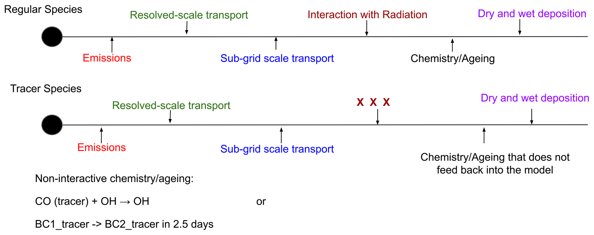
Figure 1The life cycle of a regular chemical species and a tracer chemical species is illustrated. The main difference lies in the feedback and the chemistry sections. The tracer species does not have feedback on the radiation processes in the model, and it does not affect the chemistry of regular species in the model. Two such examples of non-interactive chemistry are given. The CO tracer species gets oxidized by OH− radical, but it does not change the mass budget of the OH− radical in the model. Similarly, the tracer hydrophobic BC (BC1_tracer) species gets aged into the tracer hydrophilic BC species (BC2_tracer), while keeping the mass of the regular hydrophilic BC in the model intact.
2.4 Chemical data assimilation
DSS improves the initialization of aerosol species and thus PM2.5 field via assimilation of satellite observations of aerosol optical depth (AOD), using the three-dimensional variational (3DVAR) scheme of the community Gridpoint Statistical Interpolation system (version 3.5). The system assimilates the observations into the model by minimizing the cost function J(x) (Eq. 1), which is the sum of the deviation of the final state of the model from its background state and the observations. The cost function takes the following form:
where x is the state vector, which is composed of aerosol chemical composition and meteorological parameters needed for AOD calculation. xb is the information about x available prior to the assimilation (also known as background information). B is the background error covariance (BEC) matrix. H is the forward operator that calculates AOD from the WRF-Chem aerosol chemical composition, following Liu et al. (2011). y is the AOD retrieved by MODIS. R is the observational error covariance matrix. More details about each of the terms in Eq. (1) can be found in Kumar et al. (2020). The assimilation of MODIS AOD (from both TERRA and AQUA satellites) in the model is done at 09:00 UTC every day in the DSS. In addition to assimilation of satellite data, we also assimilate surface measurements of PM2.5 into the model at 09:00 UTC. The data come from 43 stations of the Central Pollution Control Board (CPCB) and the Delhi Pollution Control Committee (DPCC) spanning across Delhi. The exact names and the locations of the stations can be found in the supplement (their Fig. 1) of Sengupta et al. (2022).
2.5 Tagged tracers in DSS
We have added a variety of passive tagged tracers in WRF-Chem, which assist us in understanding the region- and source-specific contribution to PM2.5 mass concentration over Delhi. The passive tracer of a regular species is that species introduced in the model which undergoes all physicochemical processes identical to a regular chemical species (e.g., emissions, transport, chemical transformation, and deposition) without providing feedback to the model (Bhardwaj et al., 2021; Kumar et al., 2015). In other words, the tracer species does not take part in radiation or droplet formation processes, as its effect in such feedback processes is already taken into account by the parent regular species. The difference between a regular chemical species and a tracer chemical species is illustrated in Fig. 1.
Since PM2.5 is not a prognostic species in the model, we employ tracers for hydrophobic black carbon (BC1), hydrophilic black carbon (BC2), hydrophobic organic carbon (OC1), hydrophilic organic carbon (OC2), non-speciated primary PM2.5 (P25), and carbon monoxide (CO). The GOCART scheme employed in the WRF-Chem model used in this study calculates PM2.5 as follows:
where DUST1 is the mineral dust aerosol species falling in the first bin with the effective radii equal to 0.73 µm. DUST2 is the mineral dust aerosol species falling in the second bin with the effective radii equal to 1.4 µm. SEAS1 is the sea salt aerosol species falling in the first bin with the effective radii equal to 0.3 µm. SEAS2 is the sea salt aerosol species falling in the second bin with the effective radii equal to 1.0 µm. Sulfate is the sulfate aerosol species.
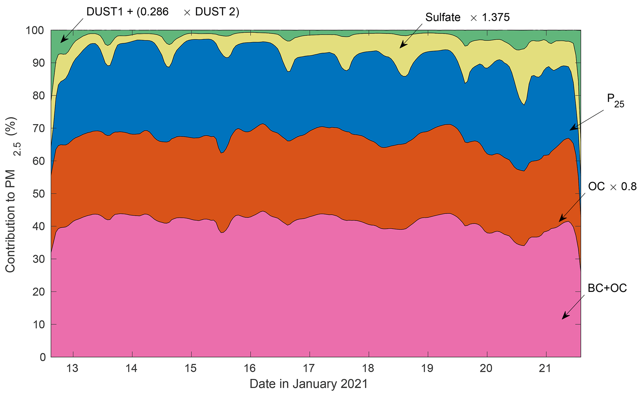
Figure 2Speciation of the WRF-Chem simulated near-surface PM2.5 mass concentration over Delhi during January 2021. Contribution from SEAS1 and SEAS2 to PM2.5 in Delhi is negligible during the study period, and thus, it is not shown in the figure.
In this study, we employ tracers for 5 of the 10 species involved in the calculation of PM2.5 in the GOCART scheme (equation 2). In Fig. 2, we examine the contribution of those 10 species to the simulated PM2.5 in the model.
It may be noted that the chosen five species (BC1, BC2, OC1, OC2, and P25) together contribute around 85 %–90 % of the total PM2.5 in the model. Thus, our five tracers would together represent, on an average, 85 %–90 % of the corresponding PM2.5 mass concentrations. Therefore, practically we can interpret those five tracers together as a PM2.5 tracer. Adding tracers for , DUST1, DUST2, SEAS1, and SEAS2 would not drastically affect the overall results, as their contribution to PM2.5 over Delhi, specifically during the winter season, is negligible, especially in the model simulations (however, the fractional contribution of different species during April–September could be different due to dust storms and monsoon circulation affecting this region). Moreover, since the forecasting system is operational on a daily basis, one needs to limit the computational load and thus the total number of species in the model configuration to keep the daily runtime as short as possible. Keeping all these constraints in mind, we chose to put tracers only for the five selected species.
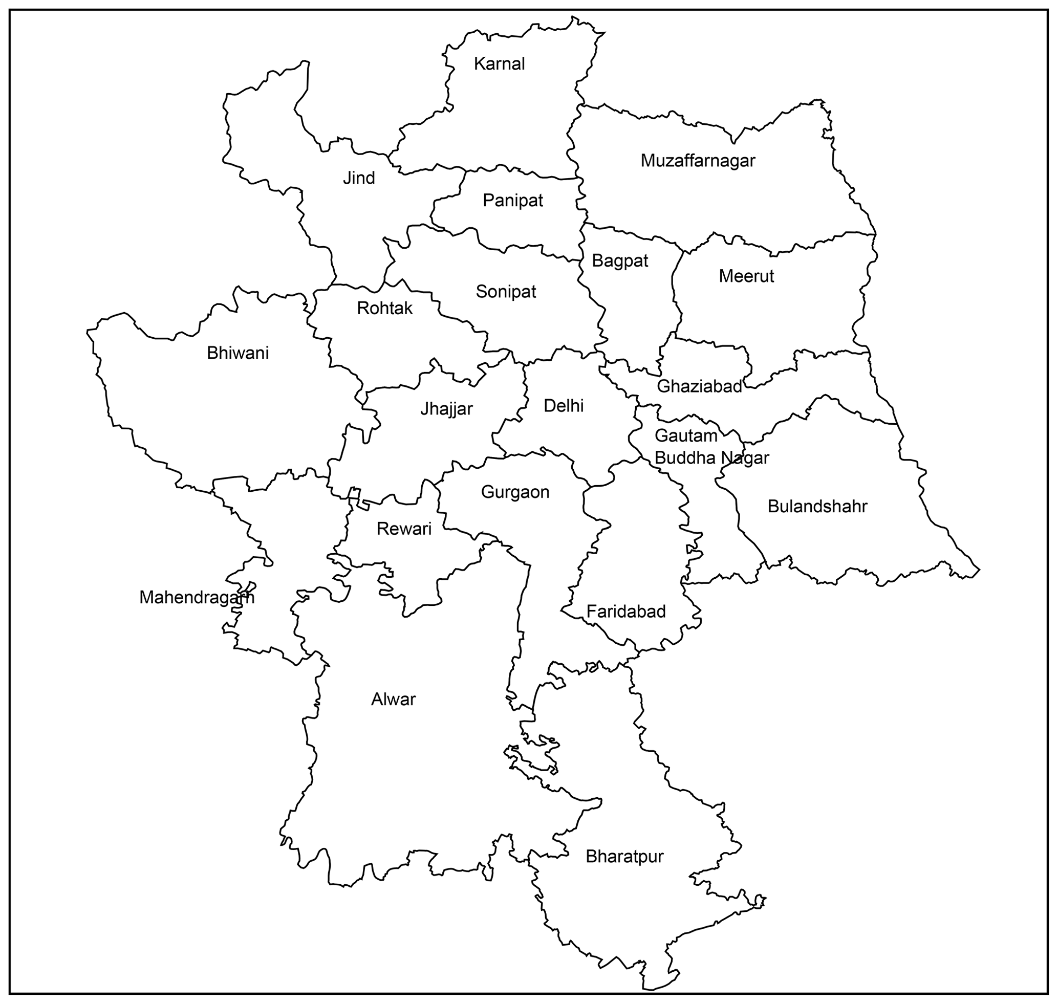
Figure 3The locations of the 20 districts of NCR whose anthropogenic PM2.5 emissions are tagged in DSS.
2.5.1 Tracers for anthropogenic PM2.5 in the model
We introduce regional tracers for the total emitted anthropogenic PM2.5 from Delhi and the 19 districts surrounding it. These districts, along with Delhi, form the NCR. The following are the districts included: Delhi, Jhajjar, Sonipat, Bagpat, Ghaziabad, Gautam Buddha Nagar, Faridabad, Gurgaon, Rohtak, Jind, Panipat, Karnal, Muzaffarnagar, Meerut, Bulandshahr, Bharatpur, Alwar, Mahendragarh, Rewari, and Bhiwani. In Fig. 3, we show the locations of these 20 districts.
Table 1The source-based PM2.5 tracers employed only for Delhi in this version of DSS. It is to be further noted that we employ tracers for the eight broad source categories (column 1) in Delhi. We do not employ tracers for the individual subcategories in this version of DSS.
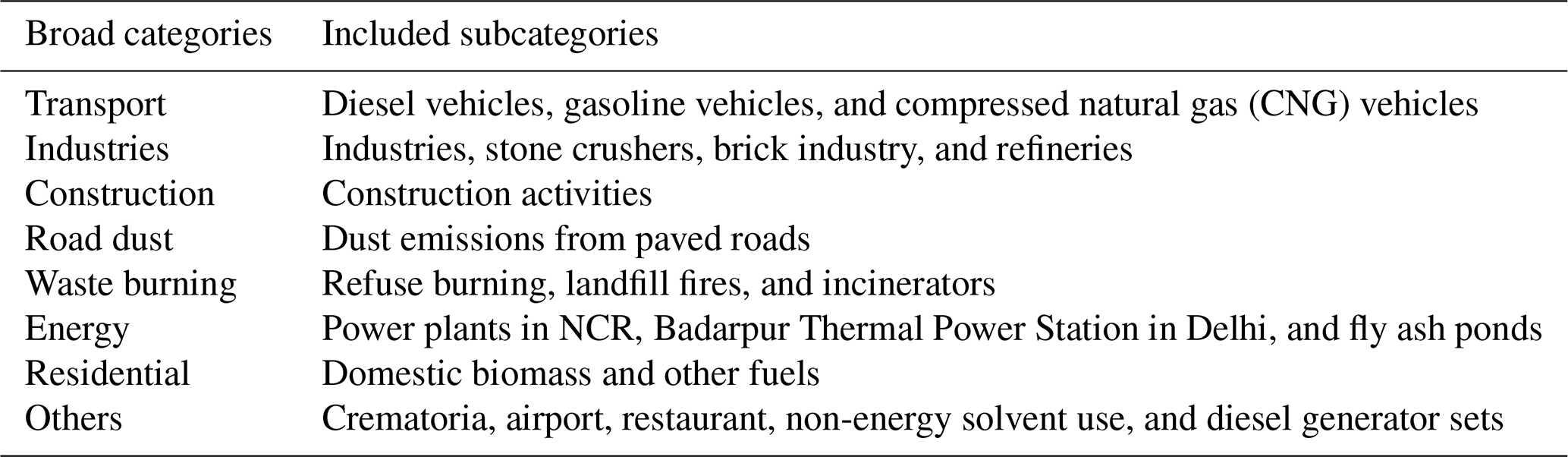
In addition to those 20 districts, we also trace PM2.5 from eight broad source-based categories exclusively in Delhi. These individual broad categories are a group of several subcategories put together. The broad categories and the included subcategories are listed in Table 1. As mentioned in Sect. 2.2, the emissions inventory provides extensive information on the subcategories for the entire NCR domain. However, version 1.0 DSS does not trace the PM2.5 emissions from the individual broad categories from the NCR districts, other than Delhi. Even for Delhi, the emissions from the individual subcategories are not traced. All these ensure the computational speed and cost for the operational DSS system. Moreover, the tagged sources fulfill the current requirements of the policymakers with regards to the air quality management in the city.
2.5.2 Tracers for biomass-burning activities
Along with the anthropogenic emissions of PM2.5, we also trace the biomass-burning-generated emissions of PM2.5. Similar to the anthropogenic PM2.5, we introduce tracers for biomass-burning-generated BC1, BC2, OC1, OC2, and P25. These tracers hold significant importance in DSS, as the post-monsoonal harvesting of paddy rice generates a large amount of stubble which gets burned and generates a thick layer of smoke in the upwind regions of Delhi, which eventually travels to Delhi. So, the tracers representing those burning activities help us identify the contribution of biomass burning to the PM2.5 load in Delhi and thus are critical for air quality management in Delhi.
2.5.3 Scenario tracers for anthropogenic PM2.5
Apart from tracing the anthropogenic and the biomass-burning-generated PM2.5, DSS offers a very unique feature, which we term scenario tracers. The scenario tracers are very similar to the other anthropogenic PM2.5 tracers, with the main difference lying in the emission magnitudes of these tracers. In DSS, a scenario tracer of a regular species has its emission 20 % or 40 % lesser than the regular species. Therefore, the scenario tracer represents a scenario in which the emissions of the corresponding regular species are reduced by 20 % or 40 %. We have introduced these scenario tracers for all the 20 districts and all the eight broad source categories in Delhi. These scenario tracers play a vital role in guiding the authorities about the possible effects of the source-level interventions. The advantage of scenario tracers is that it gives an opportunity to generate numerous emission reduction scenarios, which would guide the policymakers in finalizing the intervention targets. The use of these tracers for air quality management purposes will be shown in Sect. 3.
2.5.4 Chemical data assimilation for tracers
Another important feature of DSS is chemical data-assimilation applied for the tracer species. In DSS, for every grid point in the model domain, we identify the ratio by which the regular species like BC1, BC2, OC1, OC2, and P25 are modified due to the assimilation of satellite and ground-based data. We multiply all the corresponding tracers species by the same ratios to get them closer to reality.
2.6 Post-processing of the output
With the aforementioned tracers of different categories, we introduce a total of 470 new tracers in WRF-Chem for the purpose of DSS. Upon running DSS in an operational forecasting setup, we generate an enormous amount of data that needs to be processed to get meaningful information. In the post-processing and analysis of the output, we extract the surface-level data for all the tracers and the main regular species. Since our focus of analysis is Delhi, we mask out all other regions from the variable fields. By doing this, we estimate the contribution of PM2.5 emitted from all the regions of interest to PM2.5 in Delhi. Moreover, we also get to know the contribution from the sources in Delhi to PM2.5 in Delhi. The change in PM2.5 due to the emission reduction scenarios is subsequently found. All the analysis is made publicly available on a daily basis at https://ews.tropmet.res.in/dss/ (last access: 1 April 2024).
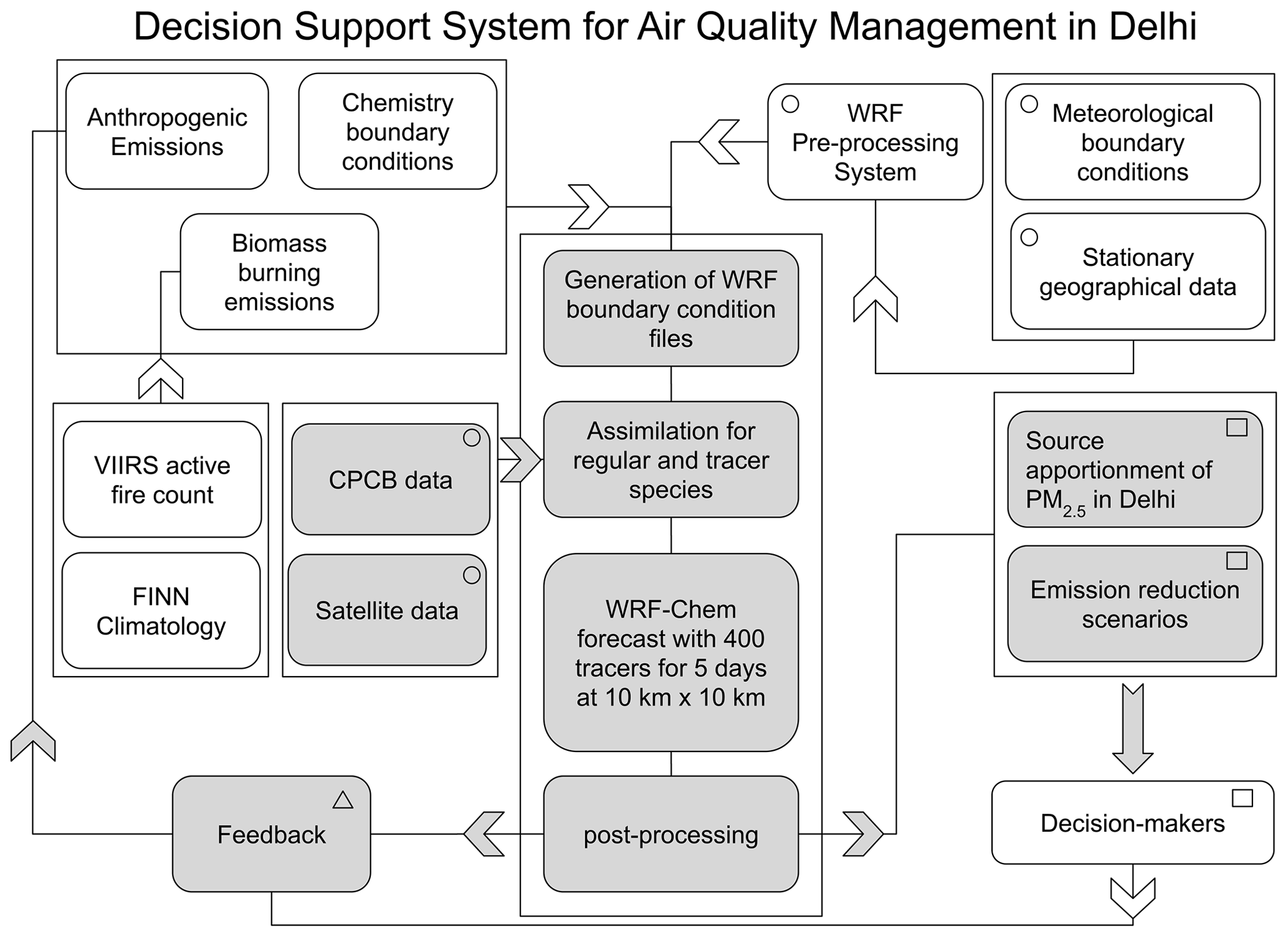
Figure 4Block diagram for DSS. The white boxes denote input data needed for the chemistry part, the white boxes with a circle in their upper-left corner stand for the input data related to the meteorological component. The gray blocks represent the core part of DSS, which is mainly related to the running of the WRF-Chem model. The gray blocks with a circle in their upper-right corner denote the input data needed for chemical-data-assimilation purposes. The gray boxes with a rectangle in their upper-right corner stand for the standard outputs from the DSS, which are communicated to the decision-makers (white block with a rectangle in its upper-right corner). The feedback (gray block with a triangle in its upper-right corner) from the decision-makers and the model's post-processed output are analyzed, and accordingly, the emissions of the anthropogenic activities are modified. A more detailed explanation of the working principle of each block can be found in Sect. 2 and 2.6.
2.7 Overall flow of DSS
Figure 4 depicts the operational functioning of DSS. The input data needed for the chemistry part (white boxes; Fig. 4), i.e., the anthropogenic and biomass-burning emissions and chemical boundary conditions, are generated using the utilities like anthro, FINN, and mozbc, as explained in Sect. 2.2 and 2.3. Note that biomass-burning emissions are generated using FINN and the VIIRS active fire count data. The meteorological input component (white boxes with a circle in their upper-left corner; Fig. 4) consists of the meteorological boundary forcing data (IITM GFS model output) and the stationary geographical data, both of which are processed by the WRF Preprocessing System (WPS) to create the model-compatible input and boundary forcing. Both the chemistry and meteorological input data are then processed by the core part of the DSS (gray boxes; Fig. 4) to create the initial and the boundary condition files. Subsequently, DSS carries out the chemical data assimilation using the CPCB and the satellite data (gray blocks with a circle in their upper-right corner; Fig. 4). After this step, the actual WRF-Chem run with 400 tracers is carried out for the next 5 d. Upon the completion of the simulation, the outputs are suitably post-processed to generate two main results (gray boxes with a rectangle in their upper-right corner; Fig. 4): (a) source apportionment of PM2.5 in Delhi to understand the contribution of the surrounding 19 districts and the 8 sectors in Delhi and (b) the effects of the various emission reduction scenarios on PM2.5 in Delhi. The results are then sent to the governing and decision-making authorities, which could take certain policy-level decisions in order to manage the air quality in Delhi. If the decision-making authorities decide to carry out certain source-level interventions (e.g., Ghude et al., 2022), then those interventions are then incorporated into the DSS through the feedback section (gray block with a triangle in its upper-right corner; Fig. 4).
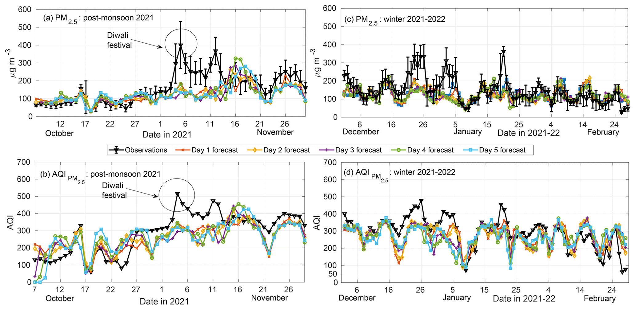
Figure 5Performance of the DSS in simulating near-surface PM2.5 mass concentration (µg m−3) over Delhi in comparison with the observations averaged over the 39 observational locations across the city. (a) Model vs. observation comparison for the simulated daily mean PM2.5 mass concentration during the post-monsoonal season of 2021. The error bars on the black line indicate the 1 standard deviation range for the observations. (b) Model vs. observation comparison for the daily mean AQI associated with PM2.5 during the post-monsoonal period. (c) Similar comparison to panel (a) for the winter season. (d) Similar to panel (b) for the winter period. The black circles mark the days of the Diwali festival during the post-monsoon period of 2021.
3.1 Performance evaluation for DSS
We examine the DSS-simulated near-surface PM2.5 mass concentration against the corresponding observations carried out at the CPCB and DPCC stations in Delhi. We divide the entire period of 5 months into the post-monsoon (October–November) and winter (December–February) seasons, as the stubble-burning activities are prevalent mainly during the post-monsoonal season, while the winter season pollution is primarily governed by the local and distant anthropogenic emissions, as well as the pollution-conducive meteorology. Thus, such a division is essential to help us understand the performance of DSS in capturing the season-specific emission sources and the associated pollutants' concentrations. We evaluate the performance of DSS for day 1 to day 5 of every day's forecasts. During the post-monsoonal period (Fig. 5a), the simulated daily mean PM2.5 closely matches the measurements for the month of October 2021. The sharp reduction in the PM2.5 during mid-October (17–20 October) is well captured by the model for all the lead times (i.e., day 1 to day 5). In the first week of November (black circles; Fig. 5a and c), the model shows a large underestimation with respect to the observations. This period was mainly associated with the peak of stubble-burning activities (Govardhan et al., 2023) and the Diwali festival in 2021. Both of these events result in emissions of a significant amount of particulate pollutants and their precursor gases (Singh et al., 2010; Parkhi et al., 2016; Cusworth et al., 2018; Chowdhury et al., 2019; Kulkarni et al., 2020; Saxena et al., 2020). The large uncertainty associated with both these emission sources (Vadrevu et al., 2015; Liu et al., 2020; Mukherjee et al., 2020; Kumar et al., 2020) results in the underestimated PM2.5 mass concentrations by DSS. The improvements in emission inventories such as the use of Fire Radiative Power (FRP) for estimating and temporally allocating fire emissions for the incorporation of emissions from fire crackers would help improve the estimates. On the contrary, the model simulations overestimate PM2.5 during the following week. Owing to the persistent severe air pollution days and a forecast of a similar scenario from 15–19 November 2021, the Government of Delhi and CAQM issued certain restrictions on the traffic in the city, banned construction activities, ordered remote schooling and working guidelines, and banned the entry of the heavy vehicles into the city (CAQM, 2022). As a result, the PM2.5 concentration in the city showed a reduction in the following week. The simulations did not implement such restrictions in the modeling framework and thus overestimated the PM2.5 concentration during this week. We further note that the fire activity in the neighboring states of Punjab and Haryana during that period was also on a declining trend (Fig. 1; Govardhan et al., 2023), so the associated fire emissions may not be completely responsible for this behavior of the model. For the entire duration, the mean overestimation is found to be 21.94 %. This overestimation is consistent with the previous estimation put forth by Ghude et al. (2022). Towards the end of November, the model captures the day-to-day variations in the observed PM2.5 but underestimates the actual magnitudes. Such a behavior could be associated with the coarse grid spacing of the model (10 km), which limits its ability to simulate higher PM concentrations. For the (Fig. 5b), the model has more of a tendency to generate AQI up to 300 (barring the episode of 15–19 November 2021). The disagreements with observations in PM2.5 get reflected in the AQI as well. It may well be noted that the model's performance does not drastically degrade from day 1 to day 5. A detailed analysis of the model's ability to capture PM2.5 and the associated AQI has been shown in Tables 2–5, which will be discussed further.
For the winter period (Fig. 5c), DSS shows a better agreement with the observation up to the middle of December, beyond which the model starts to underperform in comparison with the observations. The model simulations are capable of simulating the PM2.5 concentrations as high as 200 µg m−3; however, they are not able to simulate the higher values. Improvements in the emission inventory would be vital in this regard. This issue is likely to be related to the coarser grid spacing in the simulations, unrealistic simulations of meteorological parameters (like the planetary boundary layer height and near-surface winds) (Govardhan et al., 2015, 2016), limitations associated with the chemistry scheme in the model which may not adequately represent the ambient air pollution chemistry in Delhi (Jena et al., 2020; Pawar et al., 2023), and an underrepresentation of the emission sources in the region due to the unavailability of the real-time dynamic emissions inventory (Sengupta et al., 2022). The current emissions inventory used in the model though does have some information about the sources, like open waste burning and brick kilns in and around Delhi, but this information is likely to be underestimating the reality in 2021. The emissions inventory employed in this study was compiled using surveys done in 2016. There are significant changes that have occurred in the emissions magnitudes from 2016 to 2021. We note that these uncertainties will affect the model simulations. Moreover, during the month of January, the temperatures of the region fall down. The residents of Delhi burn biomass or solid wood for space heating purposes. Such sources are missing in the employed emissions inventory. Additionally, such burning activities occur at a very fine spatial scales, which can not be identified by remote sensing techniques. Thus, part of the underestimation during the month of January would be related to these factors. In addition to this, the lower temperatures bring foggy conditions into the picture. Such weather conditions promote a large number of atmospheric chemical reactions, resulting in gas-to-particle conversion of volatile gas phase species into secondary aerosols. Such processes are currently missing the model's chemical mechanism. This further enhances the underestimations in the model. All these factors put together result in the underestimated PM2.5 in the model vis-à-vis the measurements. Nonetheless, DSS does a better job in the month of February when the ambient PM2.5 concentration is mostly below 200 µg m−3. The is also better captured in the winter season (Fig. 5d) compared to the post-monsoon period (Fig. 5b). The model does capture some events of very poor AQI conditions (300 < AQI ≤ 400). However, the severe AQI values (AQI > 400) are missed by the model. Overall, the model captures the air quality conditions up to the very poor AQI category, but it can not quantitatively capture the severe air pollution events. However, it is also to be noted that during an observed severe air pollution event (AQI > 400), the simulated AQI lies only one category below (i.e., in the very poor AQI category). Thus, the model does show signatures of severe air pollution but fails to capture the actual magnitudes. It may also be noted that whenever the modeled AQI is in or above the very poor category, the observed AQI almost always lies in or above the very poor category; i.e., our system is able to capture extreme events very well. This point is illustrated further in Tables 4 and 5. Figure S3 in the Supplement clearly shows that the simulated AQI captures the overall trend of the observed AQI; however, the magnitudes of AQI are not captured by the model.
Table 2The statistical parameters associated with the model evaluation for the simulated near-surface PM2.5 mass concentration for the post-monsoonal season of 2021. The ideal value for all the statistical parameters is zero. The units of mean bias (MB), mean error (ME), root mean square error (RMSE) are in micrograms per cubic meter, while the other parameters of normalized mean bias (NMB), normalized mean error (NME), fractional bias (FB), and fractional error (FE) are unitless.
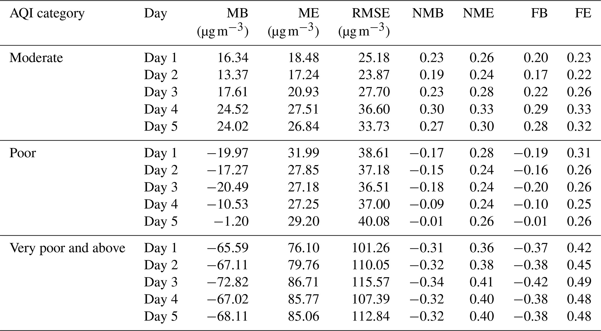
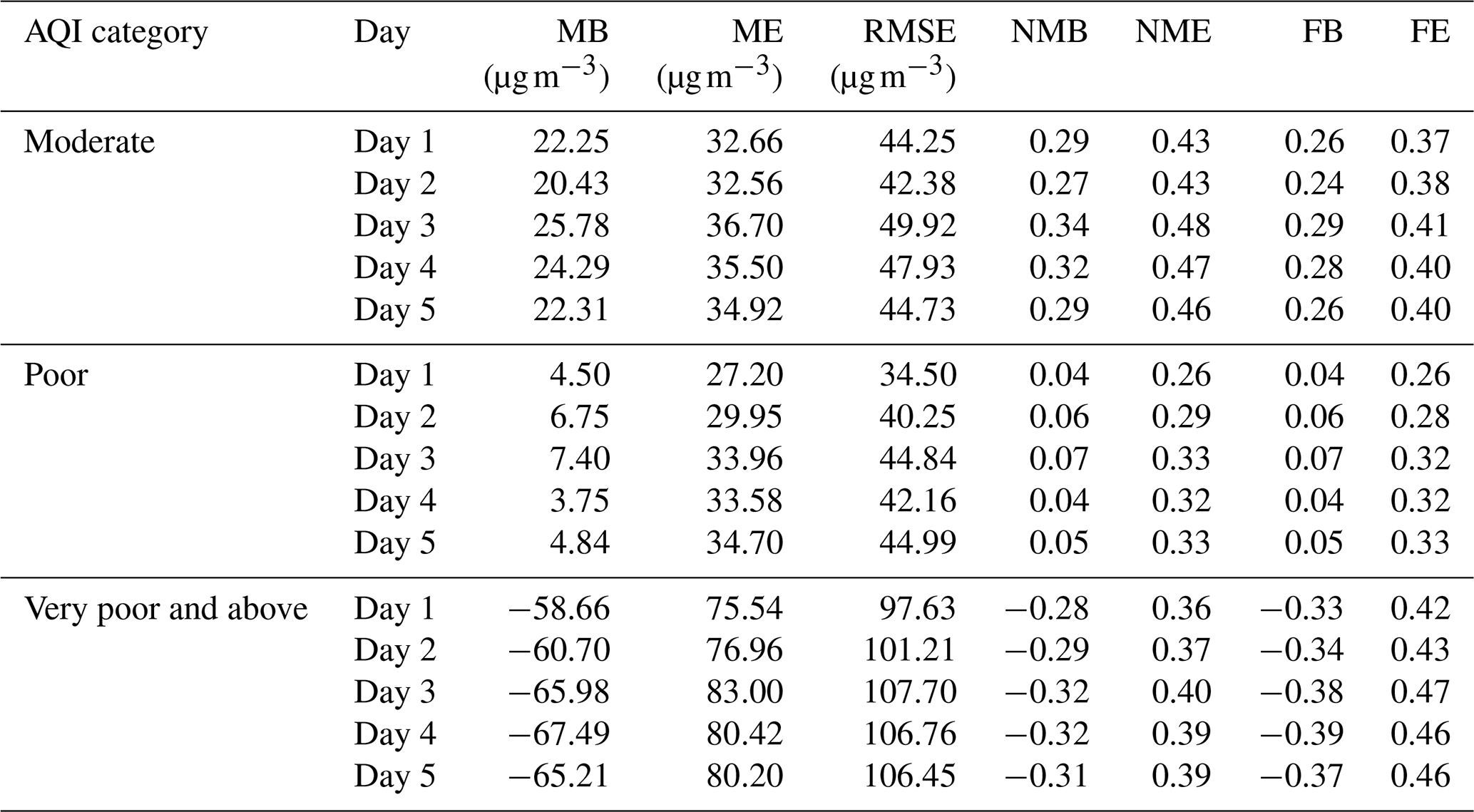
Table 3Similar to Table 2 but for the winter period of 2021–2022.
We further compute the relevant statistical parameters, namely mean bias (MB), mean error (ME), root mean square error (RMSE), normalized mean bias (NMB), normalized mean error (NME), fractional bias (FB), and fractional error (FE) for the model–observation comparison of the near-surface PM2.5 mass concentration for post-monsoon 2021 (Table 2) and winter 2021–2022 (Table 3). We report the statistics individually for moderate (100 < AQI ≤ 200), poor (200 < AQI ≤ 300), and very poor and above (AQI > 300) AQI categories for day 1 to day 5 forecasts. The formulae used for calculating the statistical parameters are listed in Sect. S4 in the Supplement. For the post-monsoon season (Table 2), DSS shows the least MB under poor AQI conditions. As expected, ME and RMSE are higher for very poor and above AQI category. Moreover, they gradually increase from day 1 to day 5 forecasts for all the scenarios. Nevertheless, the change in ME or RMSE from day 1 to day 5 is within 30 % of the ME or RMSE of day 1 forecasts, especially for the very poor and above AQI conditions. This signifies the accuracy of the forecasts over a longer time horizon. The NMB and NME values are limited to ± 0.30 and ± 0.50, suggesting that DSS depicts an acceptable accuracy for the simulated PM2.5 mass concentrations (Emery et al., 2017) for all the AQI categories through day 1 to day 5 forecasts. Specifically, NMB (NME) values do not cross 0.1 (0.37) for the poor AQI category, highlighting the accuracy of DSS and its ability to match the best model in the community (Emery et al., 2017). Like MB and NMB, FB is the least for the poor AQI conditions. The DSS tends to overpredict (underpredict) the PM2.5 with positive (negative) MB, NMB, and FB values during moderate (poor and above conditions) AQI conditions. Nevertheless, the system can simulate the observed PM2.5 during the post-monsoonal months with an acceptable deviation (Emery et al., 2017), especially when the observed AQI is in the poor or above category.
For the winter season of 2021–2022, the MB values for the moderate category (Table 3) are twice that of the post-monsoonal period, indicating a higher overestimation of the moderate AQI conditions in the model in the winter period. On the other hand, the MBs for poor and very poor and above AQI scenarios are comparable to that in the post-monsoonal months. The ME, RMSE, and NME remain roughly the same for day 1 through day 5 forecasts, which increases the trustworthiness of the forecasts on short to medium-range timescales. Similar to the post-monsoon season, the NMB and NME values for the winter season are lesser than ± 0.3 and 0.5, respectively, underscoring the ability of the system to capture the observed PM2.5 mass concentrations very adequately (Emery et al., 2017). Similarly, for the poor AQI category, the NMB and NME values are less than ± 0.1 and 0.35, respectively, suggesting an outstanding performance by DSS in this category (Emery et al., 2017). It is noteworthy that the NMB values for the very poor and above scenarios are higher compared to the poor scenario. This is likely because the very poor and above category holds a broader range of AQI values (AQI > 300) compared to the poor AQI bracket (200 < AQI ≤ 300), which results in the higher NMB in the former compared to the latter. Similar to the post-monsoonal period, the system has a tendency to overestimate (underestimate) the PM2.5 under moderate (very poor and above) AQI conditions, which is reflected in the positive (negative) MB, NMB, and FB values. Overall, the performance of the DSS is improved in the winter season compared to the post-monsoonal season (indicated by the lower values of the relevant statistical parameters in Tables 2 and 3).
Table 4The statistical parameters associated with the evaluation of the simulated AQI associated with PM2.5 mass concentration for the post-monsoonal season of 2021. Details about the formulae are mentioned in Sect. S5 in the Supplement. The ideal values for accuracy, false alarm ratio (FAR), probability of detection (POD), and critical success index (CSI) are 100.0, 0.0, 100.0, and 100.0, respectively.
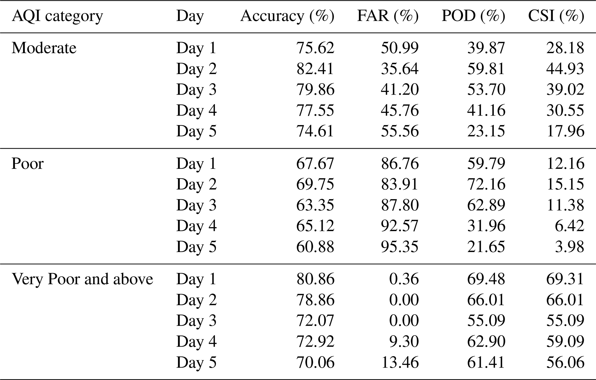
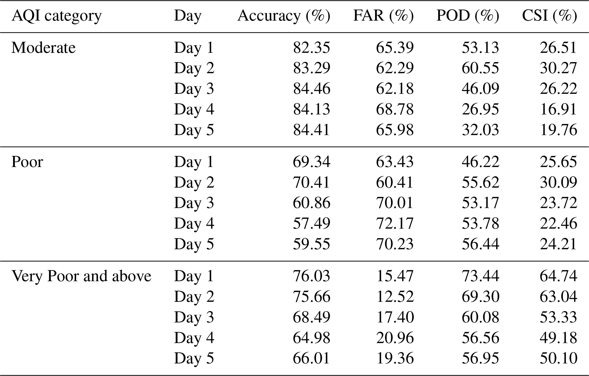
Table 5Similar to Table 4 but for the winter period of 2021–2022.
We have also examined the ability of DSS to capture the AQI associated with PM2.5 mass concentration values in comparison with the corresponding observations. To assess the model's performance, we have computed the statistical parameters, namely accuracy, false alarm ratio (FAR), probability of detection (POD), critical success index (CSI), success ratio (SR), and bias. These parameters are calculated for the individual AQI categories using the contingency table and the formulae presented in Sect. S5 in the Supplement. From Table 4, it can be seen that, during the post-monsoon season, the accuracy is generally high for all the AQI scenarios. For the poor and moderate categories, this could be an artifact of the correct forecasts of the non-events, while for the very poor and above AQI category, this behavior could be attributed to the correct forecasts for both the events and the non-events (Fig. 5b). Please note that here the term event (non-event) refers to the occurrence (non-occurrence) of the observed AQI in the desired AQI range. The probability of detection (POD) comprehends the ability of the model to give a correct forecast for occurrence of an event. On the other hand, the term accuracy, describes the ability of the model to give the correct forecast of an event or a non-event too. Thus, the term accuracy encompasses the event and non-event space, while POD covers only the event space. For the poor AQI category, it may be noted, during the post-monsoonal season (Fig. 5b) after 27 October 2021, that the observed AQI is always greater than 200, i.e., above the poor category. Thus, as far as the poor AQI category is concerned, all of those instances are recognized as non-events. The model-simulated AQI on most of those instances (if not all) is seen to be greater than 200, thus correctly giving forecasts of non-events. This correct forecasts of non-events mainly results in the respectable value of accuracy for the model forecasts as far as the poor AQI category is concerned. On the other hand, from 27 October 2021 to 30 November 2021, the POD for the poor AQI does not exist, as the observed AQI does not exist in poor category. Prior to 27 October, the observed AQI does exist in the poor category, and the model forecasts for day 4 and day 5 fail to capture that on certain occasions. This failure results in a lesser POD for day 4 and day 5 forecasts when capturing AQI in the poor category.
The FAR is higher for moderate and poor categories, suggesting false forecasts of the non-events; this could be partly related to the fact that the model-simulated AQI does not reach the very poor and above category as frequently as the observations but remains in the poor category on more instances as compared to the observations. This results in a higher FAR for the poor category. On the other hand, the FAR for the very poor and above AQI category is drastically low, which enhances the confidence in the simulated AQI in the very poor and above category. The POD is low for the poor and moderate, while it is relatively higher for the very poor and above category. The CSI values, which indicate the overall success of the forecasting system, are relatively high for the very poor and above category and lower for the poor category. Thus, during the post-monsoon season, DSS shows a trustworthy performance for the AQI ranging beyond very poor conditions.
For the winter season (Table 5), the model's behavior roughly remains the same as for the post-monsoon, with the only difference occurring in the poor AQI category. The FAR for the poor category drops with a consequent increase in CSI. Nevertheless, the model still behaves the best when AQI goes to very poor and above, with FAR being limited to as high as 21 % and the POD and CSI crossing 60 %. Thus, the analysis assures that the model-simulated AQI is trustworthy for values beyond 300.
The Graded Response Action Plan (GRAP) includes a variety of predefined temporary emission control measures for all the PM2.5 and PM10 AQI categories. Expectedly, the GRAP regulations become more stringent when the AQI goes beyond very poor and above (CAQM, 2022). Starting from October 2022, the GRAP in Delhi has been made operational, based on the AQI forecast released by the air quality forecasting models (CAQM, 2022). The low FAR for DSS in the very poor and above category certainly increases the confidence about the simulated AQI in this range and thus permits us to use the model data to implement GRAP in the city. Additionally, the FAR values for the very poor and above category remain within 20 % for day 1 to day 5 forecasts for both seasons. This further ensures that the use of short to medium-range DSS forecasts for implementation of GRAP when AQI goes beyond very poor conditions.
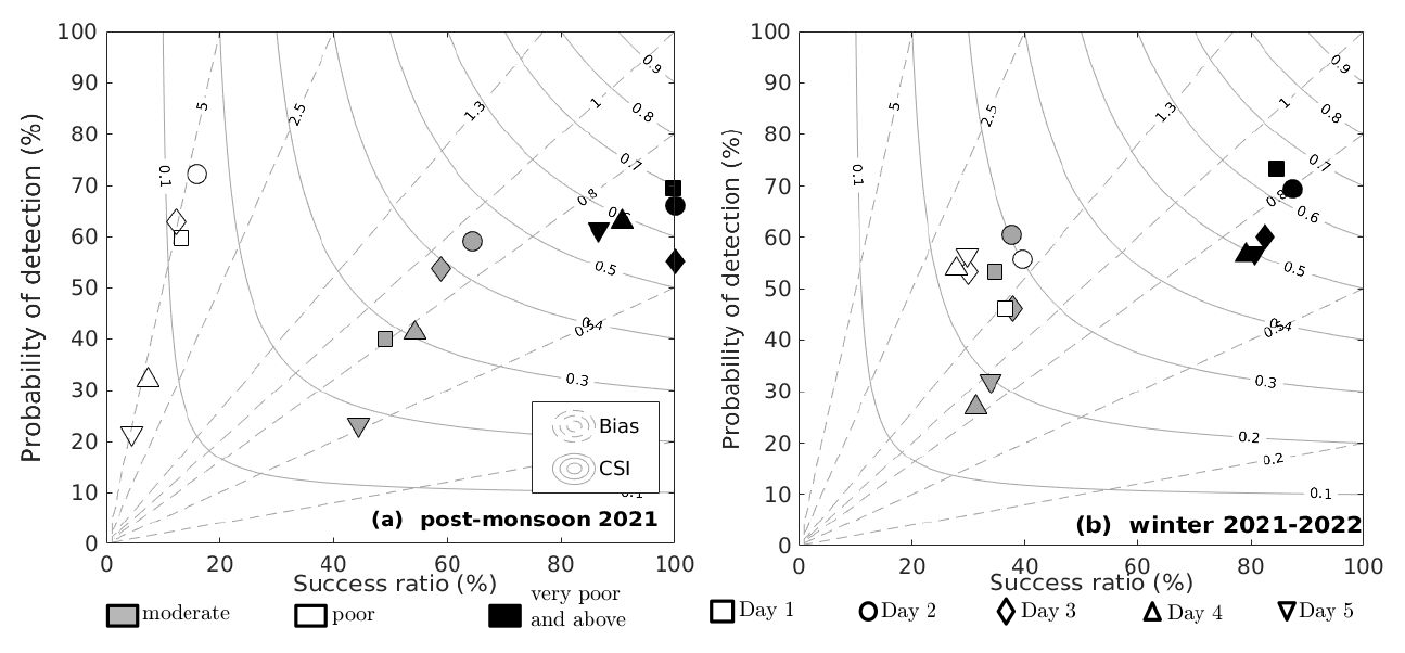
Figure 6Performance diagram for model simulations of air quality index for (a) post-monsoon season 2021 and (b) winter season 2021–2022. The details about the calculation of the statistical parameters like bias and CSI can be found in Sect. S5 in the Supplement.
To shed more light on the model's performance in the simulation of AQI, we have drawn the performance diagrams (Fig. 6) for the model simulated AQI in different categories for both seasons, using the SR, bias, CSI, and POD. The performance diagram (Roebber, 2009; Sengupta et al., 2022) provides a quick visualization of the model's performance for multiple statistical parameters. The category-wise statistical parameters have been plotted for day 1 through day 5 forecasts for the post-monsoon (Fig. 6a) and winter (Fig. 6b) seasons. In the performance diagram, an ideal model simulation would fall in the upper-right corner. It is noteworthy that the ideal value of bias is 1, which indicates that the POD and SR match each other (Roebber, 2009; Sengupta et al., 2022). This signifies that the probability of getting a false forecast for a non-event from the model is equal to that of a false forecast for an event from the same model. For the post-monsoonal period, the forecasts for very poor and above AQI fall relatively closer to the upper-right corner, with POD values going up to 70 % and SR reaching 100 %. The model is highly (moderately) skillful in capturing the very poor and above (moderate) air quality conditions. It depicts lower SR values (and thus higher FAR and Bias) for the poor AQI conditions; this is likely to be related to the underestimation of the very poor AQI by the model, resulting in higher occurrences of the simulated AQI in the poor category (in comparison with the observations), thus resulting in lower SR values for poor conditions, as noted in Table 4.
For the winter season (Fig. 6b), the model's performance shows large improvements, especially for poor AQI conditions (as noted in Table 5). The POD and SR for very poor and above conditions cross the 80 % mark, indicating an excellent performance for day 1 through day 5 forecasts. Even for the poor category, the model shows large improvements, with greater SR (∼ 40 %) and POD (∼ 60 %) values compared to the post-monsoon. Interestingly, as noted in Tables 4 and 5, for both seasons, the model shows the highest performance ratings for the very poor and above AQI conditions. The implications of this have already been discussed in the analysis of Tables 4 and 5. It is noteworthy that, throughout Sect. 3.1, we do not evaluate the model's performance for good (AQI ≤ 50) and satisfactory (50 ≤ AQI <100) categories, as the observed AQI hardly ever falls in these categories. Nonetheless, the ability of the model to capture AQI in very poor and above conditions is encouraging, as the air quality forecasting capabilities are mainly needed for such air quality conditions and not when the air quality is in good or satisfactory categories.
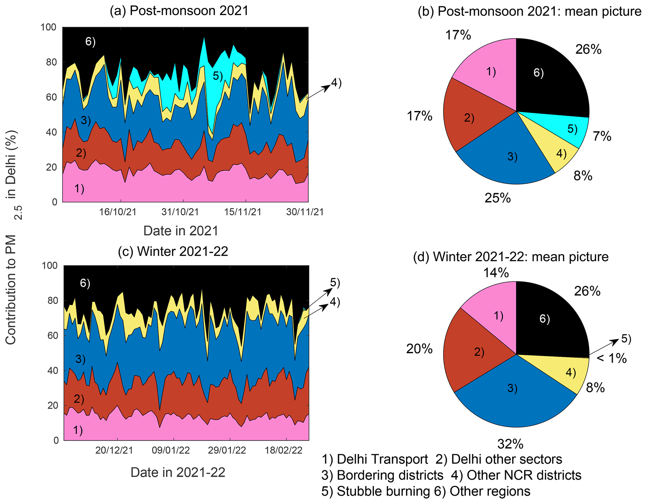
Figure 7Source apportionment of PM2.5 mass concentration in Delhi for (a) post-monsoon 2021 on a daily mean basis, (b) post-monsoon 2021 on a seasonal mean basis, (c) winter 2021–2022 on a daily mean basis, and (d) winter 2022 on a seasonal mean basis. The numbers written on the pie charts indicate the percentage contribution of the particular source to PM2.5 in Delhi. Day 1 forecasts have been used to generate this figure.
3.1.1 Region- and sector-wise source apportionment of PM2.5 in Delhi
One of the main features of DSS is its ability to quantify the contribution of the different NCR districts and emissions sources to the PM2.5 pollution load in Delhi. The tagged tracers employed in the system help achieve this objective. To facilitate ease in visualization and understanding of these contributions, we divide them in six broad categories as follows: (a) Delhi transport sector; (b) all other emission sectors within Delhi; (c) bordering districts (which include Jhajjar, Faridabad, Gurgaon, Gautam Buddha Nagar, Rohtak, Sonipat, Bagpat, and Ghaziabad districts of NCR); (d) other districts of NCR (which include the remaining districts of NCR, the details of which can be found from Fig. 3); (e) stubble burning; and (f) all other remaining regions. In Fig. 7, we show the daily mean and seasonal mean contribution of those six broad source categories to the simulated PM2.5 in Delhi for the post-monsoon and winter seasons of the year 2021. For the post-monsoonal period (Fig. 7a and b), 34 % contribution to PM2.5 in Delhi comes from Delhi's own sources, including the transport, peripheral industries, residential, construction, waste burning, road dust, and energy sectors. The next major contribution comes from the bordering districts and the stubble-burning activities, with their seasonal mean contributions going up to 25 % and 8 %, respectively. The stubble-/biomass-burning activities impact the pollution load in Delhi roughly for a month, i.e., from mid-October to mid-November. The daily mean biomass-burning contribution goes as high as 37 % in the first week of November when the biomass-burning activities in Punjab and Haryana are recorded to be at their peak (Govardhan et al., 2023). It is important to note that around 26 % of Delhi's PM2.5 comes from the other regions (excluding the biomass-burning activities), which are not included in the 20 districts considered in this analysis. Within Delhi, the major contribution comes from the transport sector, with a seasonal mean of 17 %.
During the winter season (Fig. 7c and d), Delhi's own contribution roughly remains the same (34 %). This estimate is comparable to a previous study carried out by TERI and ARAI (Automotive Research Association of India), which reports the contribution to be around 36 % (TERI and ARAI, 2018). The contribution from the neighboring districts increases to 20 % from 17 % in the post-monsoon season. Within Delhi, the transport sector contributes the highest (14 %). The industries in and around Delhi also contribute around 9.5 %. The increased contribution of the industries could be associated with the emissions coming from the brick kilns located on the periphery of the city. The kilns are not operational during the post-monsoon season, but they become operational during the winter season (TERI and ARAI, 2018). The contribution from the other regions remains roughly the same (26 %) as in the post-monsoon season. Overall, on the seasonal mean basis, for the post-monsoonal season (winter season), contributions from the different regions could be listed as follows: Delhi contributes 34.4 % (33.4 %), NCR districts contribute 33 % (40.2 %), biomass burning contributes 7.3 % (∼ 0.1 %), and the other regions contribute 27.3 % (26.4 %). Those bordering districts of Delhi contribute to around 25 % in the post-monsoon season and 32 % in the winter season. Thus a majority of the PM2.5 in Delhi comes from its immediate neighbors. Thus, Delhi's air pollution load does not look like a local issue, but it seems to be a regional issue, and cooperation among various stakeholders is required to address this problem effectively.
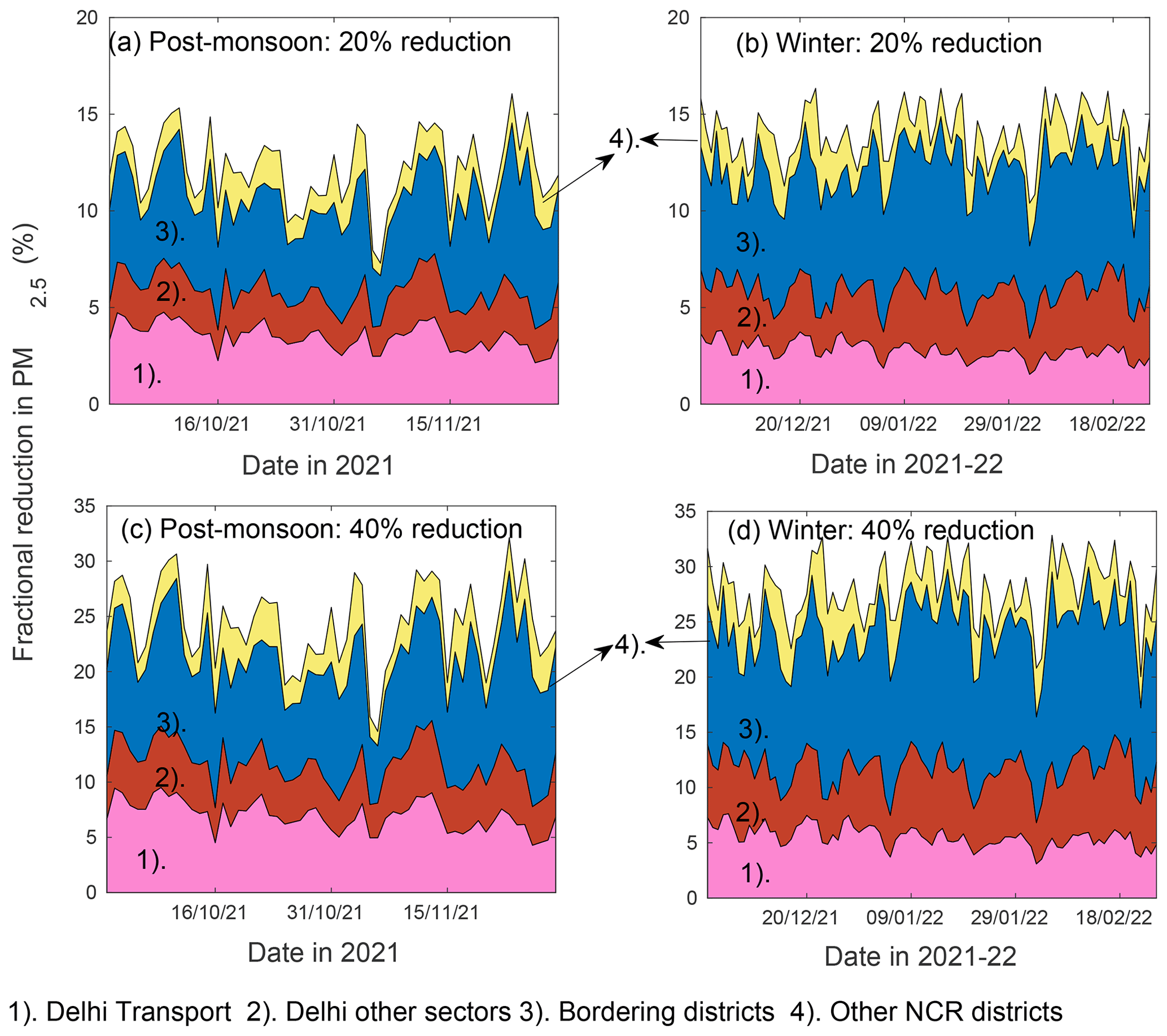
Figure 8Fractional reduction in the PM2.5 load in Delhi due to (a) a 20 % reduction in all the considered emission sources for the post-monsoon season of 2021. (b) Same as panel (a) but for the winter season. (c) Same as panel (a) but with a 40 % reduction scenario. (d) Same as panel (c) but for the winter season. Day 1 forecasts have been used to generate this figure.
3.2 Impacts of emission reductions
The most unique feature of DSS is the availability of scenario tracers. This feature estimates the impacts of reduction in the individual source- and district-wise emissions on the PM2.5 load in Delhi. We include 50 such PM2.5 tracers, which carry the reduced emissions from 25 different sources, including 19 surrounding districts and the 6 individual emission sectors (namely transport, peripheral industries, waste burning, construction, road dust, and energy) in Delhi. We form two sets of scenario tracers with (a) emissions reduced by 20 % and (b) emissions reduced by 40 %. Using the scenario tracers, one can compute the changes in the PM2.5 mass concentration in Delhi upon a 20 % or 40 % reduction in one or a combination of the 25 emissions sources (19 surrounding districts and 6 sectors in Delhi). The reduction in PM2.5 mass concentration in Delhi upon a 20 % and 40 % reduction in all those emissions during the post-monsoon and the winter seasons of 2021 have been plotted in Fig. 8. Similar to Fig. 7, we have divided the sources in four different categories i.e., categories (a) to (d) from Sect. 3.2.
During the post-monsoon season, a 20 % reduction in all the sources (Fig. 8a) results in a seasonal mean reduction of ∼ 12.1 % in PM2.5 Delhi. While around 5.7 % of it would result from a 20 % reduction in the sources within Delhi, the remaining 6.4 % would come from the reduction in the neighboring districts of NCR. Similarly, a 40 % reduction in all the concerned emissions sources (Fig. 8c) would result in an overall 24.3 % reduction in the seasonal mean PM2.5 load in Delhi, of which 11.5 % come from the reduction in the sources within Delhi, while the remaining 12.8 % would result from a 40 % reduction in the emissions from other districts of NCR. It is noteworthy that the change in PM2.5 in Delhi roughly scales linearly from a 20 % reduction to a 40 % reduction. During the period when biomass-burning activities are the highest (on 6 and 7 November 2021), the 20 % (40 %) reduction in other sources of PM2.5 reduces the PM2.5 in Delhi only by 7 %–8 % (14 %–16 %). Thus, it is noteworthy that when such activities are at their peak, any control measure on the anthropogenic emissions of PM2.5 will not have a drastic effect on the air quality in Delhi.
For the winter season, the 20 % reduction scenarios result in a mean reduction of 13.8 % in PM2.5 in Delhi, of which 5.8 % come from Delhi's sources, while the remaining 8 % come from the neighboring districts of NCR. Similarly, the 40 % reduction scenarios result in a mean reduction of 27.75 % in PM2.5 in Delhi. Out of this, 11.5 % come from Delhi's own sources, while the remaining 16.25 % come from the other districts of NCR. In the winter season, the improvements in Delhi's PM2.5 by controlling the emissions in the neighboring district of Jhajjar (see Fig. S4 in the Supplement) are comparable to the improvements achieved by controlling the transport sector emissions within Delhi. However, in the post-monsoon season, the emission reductions in Jhajjar have a relatively lesser impact. This signifies the need for change in the emission reduction strategy from season to season for air quality management in Delhi. The same policy for both seasons may not give the same results.
On a daily mean basis, the reduction scenarios can reduce the PM2.5 in Delhi by as high as 16 % (for 20 % reduction scenarios) and 32 % (for 40 % reduction scenarios) in either of the seasons. These control measures, when operated during severe air pollution events like the ones noticed during the last week of December 2021, the first week of January 2022, and the third week of January 2022 would result in a substantial reduction in Delhi's PM2.5 value. The measurements of daily mean PM2.5 suggest that the maximum values of PM2.5 during those events were 334 µg m−3, 310 µg m−3, and 362 µg m−3, respectively. The 40 % reduction scenario for all the sources would result in ∼ 25 %–30 % reduction in PM2.5 in Delhi during those days, which would roughly result in a reduction of 80–110 µg m−3 in PM2.5 in Delhi on those days. This would result in the modulation of air quality from the severe category to the very poor category. This is a satisfactory gain, considering the already elevated air pollution level in the city. Thus, such information about the possible emission-reduction scenario would be critical from the air quality management perspective. Moreover, since the performance of the DSS in capturing the broad category of air quality scenario does not drastically drop from day 1 to day 5 (Fig. 5; Tables 2–5), such information would certainly help the decision-makers in managing the air quality in the city in a timely manner.
A practical example of the use of DSS for air quality management purposes in Delhi was witnessed in the month of November 2021. Based on the air quality forecast, source attribution of PM2.5 in Delhi, and the associated scenario analysis, CAQM and the Government of Delhi issued certain restrictions on transboundary and internal vehicular traffic and construction activities in Delhi. This resulted in an 18 %–20 % reduction in PM2.5 and a 20 %–22 % reduction in the AQI of Delhi (Ghude et al., 2022). This clearly signifies the role DSS played (and would play in the future) in the short-term air quality management in Delhi. This is one of the rare air quality forecasting systems in the world that offers a utility like the scenarios tool that would inform the decision-makers about the efficacy of their source-level interventions on the air pollution occurring in a city. With the help of the scenario tool, users can create their own strategy for emission reduction to get an idea of how to possibly avoid the forecasted severe air pollution event for the city. We certainly note that DSS currently provides all such information only for the city of Delhi; however, there is an equal demand for such information from the neighboring towns of NCR like Ghaziabad, Faridabad, Noida, and Gurgaon, as outlined in the recently formed air pollution control policy for the NCR (CAQM, 2022). In the next version of DSS, we plan to cater to this requirement and explore machine-learning-based approaches to maximize computational efficiency. In the current configuration, the DSS runs with a relatively coarser resolution (10 km × 10 km). This is mainly due to the computational cost it carries associated with a large number of three-dimensional tagged tracers and the upper bound on the daily runtime due to the daily forecasting requirements. Nevertheless, in the next version, we are planning to increase the spatial resolution of the simulations. Another artifact of the coarse spatial resolution is the limited accuracy of the forecasts with respect to the observed PM2.5 values. However, in the case of DSS, one is more interested in the relative contributions of the sources to the PM2.5 load and the relative reduction in the PM2.5 upon employing the various emission reduction scenarios. This focus on the relative contribution comes from the basic assumption that the contributions would remain roughly similar, even when the DSS-simulated PM2.5 matches the observations with a greater agreement. However, we acknowledge that if the models underestimate the absolute concentration of PM2.5, it is likely to present erroneous source apportionment. Especially during a severe air quality episode in the winter season, the contribution from the local sources would be much higher, owing to the stable atmospheric conditions. In such a situation, if the model fails to capture the peak, it will certainly underestimate the contribution from the local sources and overestimate the contribution coming from the relatively distant sources. We agree that the source apportionment in that situation would not be correct. However, we would also like to mention that, in situations where the model has missed the observational peaks, the modeled attribution for the local sources would represent a lower bound than the reality. Thus, any intervention, if applied to the local sources, will certainly result in an enhanced reduction in PM2.5 in the city in reality than that suggested by the model. Thus, in other words, in such situations, the modeled source attributions and the scenario analysis would represent a lower bound.
Another reason for the underestimated PM2.5 in DSS is the static nature of the emissions inventory. However, the anthropogenic emission sources vary in a dynamic manner. Any forecasting model which does not take those dynamic changes into account is expected to miss the sudden rise in PM2.5 associated with the dynamic changes in the emissions. Even though the chemical data assimilation operational in DSS bridges this gap at the start of the model run, it fails to capture the sudden rise in emissions happening during the other hours. The incursion of the dynamic emissions inventory, though, remains a challenge; there are a few recent efforts done on that front (Liu et al., 2020; Zhang et al.,2019; Meng et al., 2020; Li et al., 2021). Using the daily Visible Infrared Imaging Radiometer Suite (VIIRS) thermal anomaly product, Zhang et al. (2019) and Li et al. (2021) have shown the capability of generating dynamic emissions for industrial sources. Meng et al. (2020) have utilized web-based traffic maps and real-time traffic data to generate a dynamic inventory of vehicular traffic emissions in China. Such techniques could be used in future versions of DSS to get better estimates of real-time traffic. The emissions inventory used in this version of DSS does not take into account emissions associated with space heating. These emissions would be non-negligible, especially in the winter months. Thus, in the next version, we would explore the possibility of including such sources of emissions.
Additionally, we do acknowledge that the model's chemistry currently lacks the representation of the secondary aerosols in the ambient air. There are several studies which have focused on understanding the chemical composition of PM2.5 in Delhi (Sharma et al., 2016; Sharma and Mandal, 2017; Jain et al., 2020; Yadav et al., 2022). A study by Sharma and Mandal (2017) reports that, the particulate organic matter, soil/crustal matter, ammonium sulphate, ammonium nitrate, sea salt, and light-absorbing carbon contribute 27.5 %, 16.1 %, 16.1 %, 13.1 %, 17.1 %, and 10.2 %, respectively, to the city's PM2.5. The study was carried out for a period of 2 years (January 2013 to December 2014). Jain et al. (2020) reported the chemical composition of PM2.5 for the period of 4 years (January 2013 to December 2016). The average PM2.5 mass concentration for post-monsoon (winter) season was 186 (183) µg m−3, out of which sulfates were reported to be 18.1 (18.6) µg m−3, nitrates were 18.4 (20.2) µg m−3, and chlorides and ammonium were 11.4 (11) and 14.9 (16.6) µg m−3, respectively. The elemental carbon and organic carbon were measured to 11.4 (10.6) and 25.2 (23.6) µg m−3, respectively. Thus, it may be seen that the missing aerosol species (mainly the nitrates, ammonium, and chlorides) in the GOCART mechanism of WRF-Chem contribute to around 24 %–30 % of PM2.5 in Delhi. Thus, part of the underestimation in the model could be associated with these missing species. An artifact of the missing secondary aerosols in the model is that the tracers are mainly put on the primary species BC and OC. However, the secondary species are not tagged effectively. This results in underestimated impacts of the source-level interventions on the ambient PM2.5. For example, in reality, the traffic emission reductions might lead to a significant reduction in nitrate aerosols, but this is not captured by the model. Thus, the model currently underestimates the impacts of source-level interventions. In the next version, we are aiming to include the missing secondary aerosols using a simple parameterization (Hodzic and Jimenez, 2011). This would include nitrate and secondary organic aerosols in the model setup without hampering the model runtime drastically.
The biomass-burning emissions, on the other hand, have even more uncertainties. The limitations associated with satellite detection of stubble-burning fires due to the cloud cover (Liu et al., 2020; Cusworth et al., 2018), the limited number of passes in a day (Liu et al., 2020; Kumar et al., 2021), smarter burning practices (Kumar et al., 2021), and unrealistic estimation of emissions from the fires (Kumar et al., 2021), leading to multiple orders of uncertainty in the emission estimates from fires. We have seen that biomass-burning fires contribute as high as 37 % to the daily mean PM2.5 load in Delhi during the peak burning periods; however, this number certainly represents a lower bound due to the aforementioned uncertainties. Therefore, more work is needed to constrain the estimates of the emissions from biomass-burning activities in the region. Additionally, stronger policies are needed to reduce the amount of stubble that is being burned, especially in the post-monsoonal season in this region. In DSS, we carry out the chemical data assimilation only once in the forecasting cycle in this setup; in the future, we can carry out assimilation at least twice to correct the model concentrations even at nighttimes. This will help the model capture higher PM concentrations which usually occur during the night hours due to shallower mixed layers. In the next version of DSS, we are planning to incorporate a few new scenario tracers, like the odd–even scenario for vehicular traffic, which allows only those vehicles with an odd (even) number as the last digit of their registration number on odd (even) dates to be on the road. This policy has been used by the Government of Delhi in the past to control vehicular movement and the associated emissions (Sud and Iyengar, 2016; Kumar et al., 2017; Chowdhury et al., 2019; Tiwari et al., 2018). Thus, while the first version of DSS has proven to be beneficial for the policymakers, we have identified its limitations as well, and we will attempt to overcome those limitations in the next version.
Additionally, we understand the day 4 and day 5 forecasts would be more useful for the policymakers. We acknowledge that the implementation of source-level intervention may not start from day 1, so in reality, one also needs to account for a time delay in implementing those. This is currently missing in the framework. However, we would also like to mention that including such time delays, even for the interventions only on the major sources, if not all, would substantially increase the number of tracers in the modeling framework. Currently, we have more than 400 three-dimensional tracers in an operational forecasting setup. Keeping in mind our operational commitments, we will certainly include some sense of the time delay for the scenario tracers in the next version of DSS.
In order to assist the governing authorities in managing the air quality in the capital of India, Delhi, we have designed an operational air quality forecasting framework with certain unique features that help the decision-makers to form policies for managing the air quality in the city. This newly developed Decision Support System (DSS) for air quality management in Delhi, besides forecasting the air quality in the north Indian region for the next 5 d, quantifies the contributions of the 19 surrounding districts, individual emission sectors in Delhi, and the biomass-burning activities (occurring primarily in the northwestern states of India in the post-monsoon season) to the PM2.5 mass concentration in Delhi. The system also quantifies the effects of emission source-level interventions on the forecasted air pollution in the city. Thus, with the help of DSS, the policymakers not only get a warning about future severe air pollution events but also understand the possible causes for the event and get a quantitative idea about the efficacy of the source-level interventions on the forecasted event. In this paper, we evaluated the performance of DSS in simulating the near-surface PM2.5 mass concentration and the associated air quality index in Delhi for the post-monsoon and winter seasons of 2021–2022. We also carry out the source apportionment of PM2.5 in Delhi during the two seasons. The key results are listed as follows:
-
The performance of the model in simulating the air pollution in Delhi noticeably improves from post-monsoon to the winter season, owing primarily to the uncertainty in the emission estimates from the biomass-burning activities and the anthropogenic activities during the Diwali festival, which occur in the post-monsoon season.
-
For both seasons (post-monsoon and winter), the DSS satisfactorily captures the observed air quality index (AQI) in Delhi, especially when the AQI crosses the very poor or above mark. Under such a situation, DSS depicts a very low false alarm ratio (∼ 20 %), which increases the trustworthiness of the simulated AQI. For all the AQI categories (moderate, poor, and very poor and above), DSS shows a very high accuracy (∼ 80 %). However, the critical success index for the simulated AQI is seen to be the highest for the very poor and above category; i.e., extreme pollution events are captured very well.
-
The performance of the model does not deviate largely from day 1 to day 5 forecasts, which highlights the applicability of the DSS forecasts in short- to medium-range air quality management activities.
-
The region-wise source apportionment of PM2.5 mass concentration in Delhi carried out with the help of DSS suggests that during the post-monsoon season (winter season), on average, Delhi itself contributes 34.4 % (33.4 %) to its PM2.5 load. The NCR districts contribute 31 % (40.2 %). The emissions from the biomass-burning activities on the seasonal mean basis contribute 7.3 % (∼ 0.1 %) of the PM2.5 mass in Delhi, while the other regions contribute around 27.3 % (26.4 %). The districts of NCR, which share their border with Delhi (namely Jhajjar, Gurgaon, Faridabad, Ghaziabad, Gautam Buddha Nagar, Bagpat, and Sonipat), contribute about 22 % in the post-monsoon season and 30 % in the winter season.
-
The scenario tracers employed for PM2.5 in DSS suggest that a 20 % reduction in all the tagged sources in Delhi and the NCR districts results in a seasonal mean reduction of ∼ 12 %–14 % in PM2.5 mass in Delhi. While around 5.8 % of that comes from controlling Delhi's own emission sources, the remaining comes from control measures applied in the NCR districts. As expected, during the peak biomass-burning events, such control measures on the anthropogenic emissions yield a relatively lesser gain.
-
The reduction in Delhi's PM2.5 load scales roughly linearly with the magnitude of emission reductions; i.e., the reduction in Delhi's PM2.5 for a 40 % control on the anthropogenic emission sources within Delhi and the NCR districts is roughly twice that of the reductions associated with a 20 % cut on emissions.
In short, DSS is a highly effective tool for decision-makers and the masses.
The observational data for PM2.5 from Central Pollution Control Board, India, are available from https://app.cpcbccr.com/ccr/#/caaqm-dashboard-all/caaqm-landing/caaqm-data-repository (Central Pollution Control Board, 2024). The model output is available on IITM high-performance computer and may be downloaded upon request to the corresponding authors. The model code employed in DSS is available at https://doi.org/10.6084/m9.figshare.21655883.v1 (Govardhan, 2022). The user manual for installing and running the code is available at https://doi.org/10.6084/m9.figshare.22335424.v1 (Govardhan, 2023).
The supplement related to this article is available online at: https://doi.org/10.5194/gmd-17-2617-2024-supplement.
Design and model development: GG, SDG, RK, PG, and CJ. Input dataset: SS. Analysis and interpretation of the result: GG, SDG, and RK. Figures: GG and SI. Writing original draft: GG. Modifying the draft: All authors. Project supervision: SDG, RK, RSN, and MR.
The contact author has declared that none of the authors has any competing interests.
Publisher's note: Copernicus Publications remains neutral with regard to jurisdictional claims made in the text, published maps, institutional affiliations, or any other geographical representation in this paper. While Copernicus Publications makes every effort to include appropriate place names, the final responsibility lies with the authors.
The authors would like to thank the Central Pollution Control Board (CPCB) and the Delhi Pollution Control Committee (DPCC) for providing measurement data for PM2.5, which was utilized in this study for chemical data assimilation and model evaluation purpose. The authors also thank the MODIS and VIIRS teams for providing satellite-retrieved AOD and active fire count information, respectively. The study was partially supported by Commission for Air Quality Management in the National Capital Region and its adjoining areas and National Supercomputing Mission. The authors would like to thank director at IITM for his constant support and motivation. The authors would like to thank handling editor Mohamed Salim, Tabish Ansari, and one anonymous reviewer for their constructive comments which improved the state of the paper. The simulations were carried out on Aditya supercomputer at IITM. Rajesh Kumar's contribution to this work is based upon work supported by the NSF National Center for Atmospheric Research, which is a major facility sponsored by the U.S. National Science Foundation (agreement no. 1852977) and NASA Health and Air Quality (grant no. 80NSSC22K1045).
This paper was edited by Mohamed Salim and reviewed by Tabish Ansari and one anonymous referee.
Banerjee, P., Satheesh, S. K., and Moorthy, K. K.: The unusual severe dust storm of May 2018 over northern India: Genesis, propagation, and associated conditions, J. Geophys. Res.-Atmos., 126, 1–25, https://doi.org/10.1029/2020JD032369, 2021.
Bhardwaj, P., Kumar, R., and Seddon, J.: Interstate transport of carbon monoxide and black carbon over India, Atmos. Environ., 251, 118268, https://doi.org/10.1016/j.atmosenv.2021.118268, 2021.
Bikkina, S., Andersson, A., Kirillova, E. N., Holmstrand, H., Tiwari, S., Srivastava, A. K., Bisht, D. S., and Gustafsson, Ö.: Air quality in megacity Delhi affected by countryside biomass burning, Nat. Sustain., 2, 200–205, https://doi.org/10.1038/s41893-019-0219-0, 2019.
Bray, C. D., Battye, W. H., and Aneja, V. P.: The role of biomass burning agricultural emissions in the Indo-Gangetic Plains on the air quality in New Delhi, India, Atmos. Environ., 218, 116983, https://doi.org/10.1016/j.atmosenv.2019.116983, 2019.
CAQM (Commision for Air Quality Management in the National Capital Region and the adjoining areas): Policy to Curb Air Pollution in the National Capital Region, https://caqm.nic.in/WriteReadData/LINKS/0031dcb806e-8af7-4b38-a9bc-65b91f2704cd.pdf (last access: 8 April 2024), 2022.
Census Of India 2011: Population Projections For India And States 2011–2036, in: Report Of The Technical Group On Population Projections, National Commission On Population Ministry Of Health & Family Welfare Nirman Bhawan, New Delhi – 110011, https://main.mohfw.gov.in/sites/default/files/Population Projection Report 2011-2036 - upload_compressed_0.pdf (last access: 1 April 2024), 2020.
Central Pollution Control Board: Central Control Room for Air Quality Management – All India, Central Pollution Control Board [data set], https://app.cpcbccr.com/ccr/#/caaqm-dashboard-all/caaqm-landing/caaqm-data-repository, last access: 4 April 2024.
Chakravarty, K., Vincent, V., Vellore, R., Srivastava, A. K., Rastogi, A., and Soni, V. K.: Revisiting Andhi in northern India: A case study of severe dust-storm over the urban megacity of New Delhi, Urban Climate, 37, 100825, https://doi.org/10.1016/j.uclim.2021.100825, 2021.
Chin, M., Rood, R. B., Lin, S.-J., Müller, J.-F., and Thompson, A. M.: Atmospheric sulfur cycle simulated in the global model GOCART: Model description and global properties, J. Geophys. Res., 105, 24671–24687, https://doi.org/10.1029/2000JD900384, 2000.
Chin, M., Ginoux, P., Kinne, S., Torres, O., Holben, B. N., Duncan, B. N., Martin, R. V., Logan, J. A., Higurashi, A., and Nakajima, T.: Tropospheric aerosol optical thickness from the GOCART model and comparisons with satellite and Sun photometer measurements, J. Atmos. Sci., 59, 461–483, https://doi.org/10.1175/1520-0469(2002)059<0461:TAOTFT>2.0.CO;2, 2002.
Chopra, R.: Environmental degradation in India: causes and consequences, Int. J. Appl. Environ. Sci., 11, 1593–1601, 2016.
Chowdhury, S., Dey, S., Di Girolamo, L., Smith, K. R., Pillarisetti, A., and Lyapustin, A.: Tracking ambient PM2.5 build-up in Delhi national capital region during the dry season over 15 years using a high-resolution (1km) satellite aerosol dataset, Atmos. Environ., 204, 142–150, https://doi.org/10.1016/j.atmosenv.2019.02.029, 2019.
Clough, S. A., Shephard, M. W., Mlawer, E. J., Delamere, J. S., Iacono, M. J., Cady-Pereira, K., Boukabara, S., and Brown, P. D.: Atmospheric radiative transfer modeling: A summary of the AER codes, J. Quant. Spectrosc. Ra, 91, 233–244, https://doi.org/10.1016/j.jqsrt.2004.05.058, 2005.
Colette, A., Rouïl, L., Meleux, F., Lemaire, V., and Raux, B.: Air Control Toolbox (ACT_v1.0): a flexible surrogate model to explore mitigation scenarios in air quality forecasts, Geosci. Model Dev., 15, 1441–1465, https://doi.org/10.5194/gmd-15-1441-2022, 2022.
Cusworth, D. H., Mickley, L. J., Sulprizio, M. P., Liu, T., Marlier, M. E., DeFries, R. S., Guttikunda, S. K., and Gupta, P.: Quantifying the influence of agricultural fires in northwest India on urban air pollution in Delhi, India, Environ. Res. Lett., 13, 044018, https://doi.org/10.1088/1748-9326/aab303, 2018.
Debnath, S., Jena, C., Ghude, S. D., Kumar, R., Govardhan, G., Gunwani, P., Saha, S. K., Hazra, A., and Pokhrel, S.: Simulation of Indian Summer Monsoon Rainfall (ISMR) with fully coupled regional chemistry transport model: A case study for 2017, Atmos. Environ., 268, 118785, https://doi.org/10.1016/j.atmosenv.2021.118785, 2022.
Denby, B. R., Gauss, M., Wind, P., Mu, Q., Grøtting Wærsted, E., Fagerli, H., Valdebenito, A., and Klein, H.: Description of the uEMEP_v5 downscaling approach for the EMEP MSC-W chemistry transport model, Geosci. Model Dev., 13, 6303–6323, https://doi.org/10.5194/gmd-13-6303-2020, 2020.
Ek, M. B., Mitchell, K. E., Lin, Y., Rogers, E., Grunmann, P., Koren, V., Gayno, G., and Tarpley, J. D.: Implementation of Noah land surface model advances in the National Centers for Environmental Prediction operational mesoscale Eta model, J. Geophys. Res.-Atmos., 108, 8851, https://doi.org/10.1029/2002JD003296, 2003.
Emery, C., Liu, Z., Russell, A. G., Odman, M. T., Yarwood, G., and Kumar, N.: Recommendations on statistics and benchmarks to assess photochemical model performance, JAPCA J. Air Waste Ma., 67, 582–598, https://doi.org/10.1080/10962247.2016.1265027,2017.
Emmons, L. K., Walters, S., Hess, P. G., Lamarque, J.-F., Pfister, G. G., Fillmore, D., Granier, C., Guenther, A., Kinnison, D., Laepple, T., Orlando, J., Tie, X., Tyndall, G., Wiedinmyer, C., Baughcum, S. L., and Kloster, S.: Description and evaluation of the Model for Ozone and Related chemical Tracers, version 4 (MOZART-4), Geosci. Model Dev., 3, 43–67, https://doi.org/10.5194/gmd-3-43-2010, 2010.
Gadi, R., Shivani, Sharma, S. K., and Mandal, T. K.: Source apportionment and health risk assessment of organic constituents in fine ambient aerosols (PM2.5): a complete year study over National Capital Region of India, Chemosphere, 221, 583–596, https://doi.org/10.1016/j.chemosphere.2019.01.067, 2019.
Ghude, S. D., Chate, D. M., Jena, C., Beig, G., Kumar, R., Barth, M. C., Pfister, G. G., Fadnavis, S., and Pithani, P.: Premature mortality in India due to PM2.5 and ozone exposure, Geophys. Res. Lett., 43, 4650–4658, https://doi.org/10.1002/2016GL068949, 2016.
Ghude, S. D., Kumar, R., Jena, C., Debnath, S., Kulkarni, R. G., Alessandrini, S., Biswas, M., Kulkrani, S., Pithani, P., Kelkar, S., and Sajjan, V.: Evaluation of PM2.5 forecast using chemical data assimilation in the WRF-Chem model: A novel initiative under the Ministry of Earth Sciences Air Quality Early Warning System for Delhi India, Curr. Sci., 118, 1803–1815, https://doi.org/10.18520/cs/v118/i11/1803-1815, 2020.
Ghude, S. D., Kumar, R., Govardhan, G., Jena, C., Nanjundiah, R. S., and Rajeevan, M.: New Delhi: air-quality warning system cuts peak pollution, Nature, 602, 211–211, https://doi.org/10.1038/d41586-022-00332-y, 2022.
Ginoux, P., Chin, M., Tegen, I., Prospero, J. M., Holben, B., Dubovik, O., and Lin, S.-J.: Sources and distributions of dust aerosols simulated with the GOCART model. J. Geophys. Res., 106, 20255–20273, https://doi.org/10.1029/2000JD000053, 2001.
Govardhan, G.: WRF-Chem-DSS-Model, figshare [software], https://doi.org/10.6084/m9.figshare.21655883.v1, 2022.
Govardhan, G.: User manual for WRF-Chem based DSS for air quality management, figshare [software], https://doi.org/10.6084/m9.figshare.22335424.v1, 2023.
Govardhan, G., Nanjundiah, R. S., Satheesh, S. K., Krishnamoorthy, K., and Kotamarthi, V. R.: Performance of WRF-Chem over Indian region: Comparison with measurements, J. Earth Syst. Sci., 124, 875–896, https://www.ias.ac.in/article/fulltext/jess/124/04/0875-0896 (last access: 4 April 2024), 2015.
Govardhan, G., Satheesh, S. K., Moorthy, K. K., and Nanjundiah, R.: Simulations of black carbon over the Indian region: improvements and implications of diurnality in emissions, Atmos. Chem. Phys., 19, 8229–8241, https://doi.org/10.5194/acp-19-8229-2019, 2019.
Govardhan, G., Ambulkar, R., Kulkarni, S., Vishnoi, A., Yadav, P., Chowdhury, B. A., Khare, M., and Ghude, S. D.: Stubble-burning activities in north-western India in 2021: Contribution to air pollution in Delhi, Heliyon, 9, e16939, https://doi.org/10.1016/J.HELIYON.2023.E16939, 2023.
Govardhan, G. R., Nanjundiah, R. S., Satheesh, S. K., Moorthy, K. K., and Takemura, T.: Inter-comparison and performance evaluation of chemistry transport models over Indian region, Atmos. Environ., 125, 486–504, https://doi.org/10.1016/j.atmosenv.2015.10.065, 2016.
Grell, G. A. and Freitas, S. R.: A scale and aerosol aware stochastic convective parameterization for weather and air quality modeling, Atmos. Chem. Phys., 14, 5233–5250, https://doi.org/10.5194/acp-14-5233-2014, 2014.
Grell, G. A., Peckham, S. E., Schmitz, R., McKeen, S. A., Frost, G., Skamarock, W. C., and Eder, B.: Fully coupled “online” chemistry within the WRF model, Atmos. Environ., 39, 6957–6975, 2005.
Guo, H., Kota, S. H., Chen, K., Sahu, S. K., Hu, J., Ying, Q., Wang, Y., and Zhang, H.: Source contributions and potential reductions to health effects of particulate matter in India, Atmos. Chem. Phys., 18, 15219–15229, https://doi.org/10.5194/acp-18-15219-2018, 2018.
Guo, H., Kota, S. H., Sahu, S. K., and Zhang, H.: Contributions of local and regional sources to PM2.5 and its health effects in north India, Atmos. Environ., 214, 116867, https://doi.org/10.1016/j.atmosenv.2019.116867, 2019.
Guttikunda, S. K. and Goel, R.: Health impacts of particulate pollution in a megacity-Delhi, India, Environ. Dev., 6, 8–20, https://doi.org/10.1016/j.envdev.2012.12.002, 2013.
Guttikunda, S. K. and Gurjar, B. R.: Role of meteorology in seasonality of air pollution in megacity Delhi, India, Environ. Monit. Assess., 184, 3199–3211, https://doi.org/10.1007/s10661-011-2182-8, 2012.
Hama, S., Kumar, P., Alam, M. S., Rooney, D. J., Bloss, W. J., Shi, Z., Harrison, R. M., Crilley, L. R., Khare, M., and Gupta, S. K.: Chemical source profiles of fine particles for five different sources in Delhi, Chemosphere, 274, https://doi.org/10.1016/j.chemosphere.2021.129913, 2021.
Hodzic, A. and Jimenez, J. L.: Modeling anthropogenically controlled secondary organic aerosols in a megacity: a simplified framework for global and climate models, Geosci. Model Dev., 4, 901–917, https://doi.org/10.5194/gmd-4-901-2011, 2011.
Hong, S. Y. and Lim, J. O. J.: The WRF single-moment 6-class microphysics scheme (WSM6), Asia-Pac. J. Atmos. Sci., 42, 129–151, 2006.
Iacono, M. J., Mlawer, E. J., Clough, S. A., and Morcrette, J.-J.: Impact of an improved longwave radiation model, rrtm, on the energy budget and thermodynamic properties of the ncar community climate model ccm3, J. Geophys. Res., 105, 14873–14890, https://doi.org/10.1029/2000JD900091, 2000.
Iacono, M. J., Delamere, J. S., Mlawer, E. J., Shephard, M. W., Clough, S. A., and Collins, W. D.: Radiative forcing by long-lived greenhouse gases: Calculations with the aer radiative transfer models, J. Geophys. Res., 113, 1–8, https://doi.org/10.1029/2008JD009944, 2008.
Jain, S., Sharma, S. K., Vijayan, N., and Mandal, T. K.: Seasonal characteristics of aerosols (PM2.5 and PM10) and their source apportionment using PMF: a four year study over Delhi, India, Environ. Pollut., 262, 114337, https://doi.org/10.1016/j.envpol.2020.114337, 2020.
Janssens-Maenhout, G., Crippa, M., Guizzardi, D., Dentener, F., Muntean, M., Pouliot, G., Keating, T., Zhang, Q., Kurokawa, J., Wankmüller, R., Denier van der Gon, H., Kuenen, J. J. P., Klimont, Z., Frost, G., Darras, S., Koffi, B., and Li, M.: HTAP_v2.2: a mosaic of regional and global emission grid maps for 2008 and 2010 to study hemispheric transport of air pollution, Atmos. Chem. Phys., 15, 11411–11432, https://doi.org/10.5194/acp-15-11411-2015, 2015.
Jena, C., Ghude, S. D., Kulkarni, R., Debnath, S., Kumar, R., Soni, V. K., Acharja, P., Kulkarni, S. H., Khare, M., Kaginalkar, A. J., Chate, D. M., Ali, K., Nanjundiah, R. S., and Rajeevan, M. N.: Evaluating the sensitivity of fine particulate matter (PM2.5) simulations to chemical mechanism in Delhi, Atmos. Chem. Phys. Discuss. [preprint], https://doi.org/10.5194/acp-2020-673, 2020.
Jena, C., Ghude, S. D., Kumar, R., Debnath, S., Govardhan, G., Soni, V. K., Kulkarni, S. H., Beig, G., Nanjundiah, R. S., and Rajeevan, M.: Performance of high resolution (400 m) PM2.5 forecast over Delhi, Sci. Rep.-UK, 11, 4104, https://www.nature.com/articles/s41598-021-83467-8 (last access: 4 April 2024), 2021.
Jiménez, P. A., Dudhia, J., González-Rouco, J. F., Navarro, J., Montávez, J. P., and García-Bustamante, E.: A revised scheme for the WRF surface layer formulation, Mon. Weather Rev., 140, 898–918, https://doi.org/10.1175/MWR-D-11-00056.1, 2012.
Kaiser, J. W., Heil, A., Andreae, M. O., Benedetti, A., Chubarova, N., Jones, L., Morcrette, J.-J., Razinger, M., Schultz, M. G., Suttie, M., and van der Werf, G. R.: Biomass burning emissions estimated with a global fire assimilation system based on observed fire radiative power, Biogeosciences, 9, 527–554, https://doi.org/10.5194/bg-9-527-2012, 2012.
Kanawade, V. P., Srivastava, A. K., Ram, K., Asmi, E., Vakkari, V., Soni, V. K., Varaprasad, V., and Sarangi, C.: What caused severe air pollution episode of November 2016 in New Delhi?, Atmos. Environ., 222, 117125, https://doi.org/10.1016/j.atmosenv.2019.117125, 2020.
Kulkarni, S. H., Ghude, S. D., Jena, C., Karumuri, R. K., Sinha, B., Sinha, V., Kumar, R., Soni, V. K., and Khare, M.: How Much Does Large-Scale Crop Residue Burning Affect the Air Quality in Delhi?, Environ. Sci. Technol., 54, 4790–4799, https://doi.org/10.1021/ACS.EST.0C00329, 2020.
Kumar, A., Hakkim, H., Sinha, B., and Sinha, V.: Gridded 1 km × 1 km emission inventory for paddy stubble burning emissions over north-west India constrained by measured emission factors of 77 VOCs and district-wise crop yield data, Sci. Total Environ., 789, 148064, https://doi.org/10.1016/j.scitotenv.2021.148064, 2021.
Kumar, P., Gulia, S., Harrison, R. M., and Khare, M.: The influence of odd–even car trial on fine and coarse particles in Delhi, Environ. Pollut., 225, 20–30, https://doi.org/10.1016/j.envpol.2017.03.017, 2017.
Kumar, R., Ghude, S. D., Biswas, M., Jena, C., Alessandrini, S., Debnath, S., Kulkarni, S., Sperati, S., Soni, V. K., Nanjundiah, R. S., and Rajeevan, M.: Enhancing accuracy of air quality and temperature forecasts during paddy crop residue burning season in Delhi via chemical data assimilation, J. Geophys. Res.-Atmos., 125, 1–16, https://doi.org/10.1029/2020JD033019, 2020.
Lalchandani, V., Kumar, V., Tobler, A., M. Thamban, N., Mishra, S., Slowik, J. G., Bhattu, D., Rai, P., Satish, R., Ganguly, D., Tiwari, S., Rastogi, N., Tiwari, S., Močnik, G., Prévôt, A. S. H., and Tripathi, S. N.: Real-time characterization and source apportionment of fine particulate matter in the Delhi megacity area during late winter, Sci. Total Environ., 770, 145324, https://doi.org/10.1016/j.scitotenv.2021.145324, 2021.
Li, R., Tao, M., Zhang, M., Chen, L., Wang, L., Wang, Y., He, X., Wei, L., Mei, X., and Wang, J.: Application potential of satellite thermal anomaly products in updating industrial emission inventory, Geophys. Res. Lett., 48, 1–7, https://doi.org/10.1029/2021GL092997, 2021.
Liu, T., Mickley, L. J., Singh, S., Jain, M., Defries, R. S., and Marlier, M. E.: Crop residue burning practices across north India inferred from household survey data: Bridging gaps in satellite observations, Atmos. Environ., 8, 100091, https://doi.org/10.1016/j.aeaoa.2020.100091, 2020.
Liu, Y., Hu, C., Zhan, W., Sun, C., Murch, B., and Ma, L.: Identifying industrial heat sources using time-series of the VIIRS Night fire product with an object-oriented approach, Remote Sens. Environ., 204, 347–365, https://doi.org/10.1016/j.rse.2017.10.019, 2018.
Liu, Z., Liu, Q., Lin, H.-C., Schwartz, C. S., Lee, Y.-H., and Wang, T.: Three-dimensional variational assimilation of MODIS aerosol optical depth: Implementation and application to a dust storm over East Asia, J. Geophys. Res., 116, 1–19, https://doi.org/10.1029/2011JD016159, 2011.
Meng, X., Zhang, K., Pang, K., and Xiang, X.: Characterization of spatio-temporal distribution of vehicle emissions using web-based real-time traffic data, Sci. Total Environ., 709, 136227, https://doi.org/10.1016/j.scitotenv.2019.136227, 2020.
Meteosim: World Most Polluted Cities – Meteosim (WWW Document), Meteosim, https://www.meteosim.com/en/world-most-polluted-citie/ (last access: 5 April 2024), 2019.
Mlawer, E. J., Taubman, S. J., Brown, P. D., Iacono, M. J., and Clough, S. A.: Radiative transfer for inhomogeneous atmospheres: RRTM, a validated correlated-k model for the longwave, J. Geophys. Res.-Atmos., 102, 16663–16682, https://doi.org/10.1029/97JD00237, 1997.
Molina, M. J. and Molina, L. T.: Megacities and atmospheric pollution, J. Air Waste Manage., 54, 644–680, https://doi.org/10.1080/10473289.2004.10470936, 2004.
Mukherjee, T., Vinoj, V., Midya, S. K., Puppala, S. P., and Adhikary, B.: Numerical simulations of different sectoral contributions to post-monsoon pollution over Delhi, Heliyon, 6, e03548, https://doi.org/10.1016/j.heliyon.2020.e03548, 2020.
Mukhopadhyay, P., Prasad, V. S., Krishna, R., Deshpande, M., Ganai, M., Tirkey, S., Sarkar, S., Goswami, T., Johny, C. J., Roy, K., Mahakur, M., Durai V. R., and Rajeevan, M.: Performance of a very high-resolution global forecast system model (GFS T1534) at 12.5 km over the Indian region during the 2016–2017 monsoon seasons, J. Earth Syst. Sci., 128, 1–18, https://doi.org/10.1007/s12040-019-1186-6, 2019.
Nair, M., Bherwani, H., Kumar, S., Gulia, S., Goyal, S., and Kumar, R.: Assessment of contribution of agricultural residue burning on air quality of Delhi using remote sensing and modelling tools, Atmos. Environ., 230, 117504, https://doi.org/10.1016/j.atmosenv.2020.117504, 2020.
Nakanishi, M. and Niino, H.: An Improved Mellor–Yamada Level-3 Model: Its Numerical Stability and Application to a Regional Prediction of Advection Fog, Bound. Lay. Meteorol., 119, 397–407, https://doi.org/10.1007/s10546-005-9030-8, 2006.
Niu, G. Y., Yang, Z. L., Mitchell, K. E., Chen, F., Ek, M. B., Barlage, M., Kumar, A., Manning, K., Niyogi, D., Rosero, E., and Tewari, M.: The community Noah land surface model with multi parameterization options (Noah-MP): 1. Model description and evaluation with local-scale measurements, J. Geophys. Res.-Atmos., 116, 1–19, https://doi.org/10.1029/2010JD015140, 2011.
Parde, A. N., Dhangar, N. G., Nivdange, S., Ghude, S. D., Pithani, P., Jena, C., Lal, D. M., and Gopalakrishnan, V.: The analysis of pre-monsoon dust storm over Delhi using ground-based observations, Nat. Hazards, 112, 829–844, https://doi.org/10.1007/s11069-022-05207-z, 2022.
Parkhi, N., Chate, D., Ghude, S. D., Peshin, S., Mahajan, A., Srinivas, R., Surendran, D., Ali, K., Singh, S., Trimbake, H., and Beig, G.: Large inter annual variation in air quality during the annual festival “Diwali” in an Indian megacity, J. Environ. Sci., 43, 265–272, https://doi.org/10.1016/j.jes.2015.08.015, 2016.
Pawar, P. V., Ghude, S. D., Govardhan, G., Acharja, P., Kulkarni, R., Kumar, R., Sinha, B., Sinha, V., Jena, C., Gunwani, P., Adhya, T. K., Nemitz, E., and Sutton, M. A.: Chloride (HCl / Cl−) dominates inorganic aerosol formation from ammonia in the Indo-Gangetic Plain during winter: modeling and comparison with observations, Atmos. Chem. Phys., 23, 41–59, https://doi.org/10.5194/acp-23-41-2023, 2023.
Rai, P., Furger, M., el Haddad, I., Kumar, V., Wang, L., Singh, A., Dixit, K., Bhattu, D., Petit, J. E., Ganguly, D., Rastogi, N., Baltensperger, U., Tripathi, S. N., Slowik, J. G., and Prévôt, A. S. H.: Real-time measurement and source apportionment of elements in Delhi's atmosphere, Sci. Total Environ., 742, 140332, https://doi.org/10.1016/j.scitotenv.2020.140332, 2020.
Riahi, K., Van Vuuren, D. P., Kriegler, E., Edmonds, J., O'neill, B. C., Fujimori, S., Bauer, N., Calvin, K., Dellink, R., Fricko, O., and Lutz, W.: The shared socioeconomic pathways and their energy, land use, and greenhouse gas emissions implications: an overview, Global Environ. Chang., 42, 153–168, https://doi.org/10.1016/j.gloenvcha.2016.05.009, 2017.
Roebber, P. J.: Visualizing multiple measures of forecast quality, Weather Forecast, 24, 601–608, https://doi.org/10.1175/2008WAF2222159.1, 2009.
Roozitalab, B., Carmichael, G. R., and Guttikunda, S. K.: Improving regional air quality predictions in the Indo-Gangetic Plain – case study of an intensive pollution episode in November 2017, Atmos. Chem. Phys., 21, 2837–2860, https://doi.org/10.5194/acp-21-2837-2021, 2021.
Sahu, S. K., Mangaraj, P., and Beig, G.: Decadal growth in emission load of major air pollutants in Delhi, Earth Syst. Sci. Data, 15, 3183–3202, https://doi.org/10.5194/essd-15-3183-2023, 2023.
Saini, P. and Sharma, M.: Cause and Age-specific premature mortality attributable to PM2.5 Exposure: An analysis for Million-Plus Indian cities, Sci. Total Environ., 710, 135230, https://doi.org/10.1016/j.scitotenv.2019.135230, 2020.
Saxena, P., Srivastava, A., Verma, S., Singh, L., and Sonwani, S.: Analysis of atmospheric pollutants during fireworks festival “`Diwali” at a residential site Delhi in India, in: Energy, Environment, and Sustainability, Springer, 91–105, https://doi.org/10.1007/978-981-15-0540-9_4, 2020.
Schroeder, W., Oliva, P., Giglio, L., and Csiszar, I. A.: The New VIIRS 375 m active fire detection data product: algorithm description and initial assessment, Remote Sens Environ., 143, 85–96, https://doi.org/10.1016/j.rse.2013.12.008, 2014.
Sengupta, A., Govardhan, G., Debnath, S., Yadav, P., Kulkarni, S. H., Parde, A. N., Lonkar, P., Dhangar, N., Gunwani, P., Wagh, S., Nivdange, S., Jena, C., Kumar, R., and Ghude, S. D.: Probing into the wintertime meteorology and particulate matter (PM2.5 and PM10) forecast over Delhi, Atmos. Pollut. Res., 13, 101426, https://doi.org/10.1016/j.apr.2022.101426, 2022.
Sharma, S. K. and Mandal, T. K.: Chemical composition of fine mode particulate matter (PM2.5) in an urban area of Delhi, India and its source apportionment, Urban Climate, 21, 106–122, https://doi.org/10.1016/j.uclim.2017.05.009, 2017.
Sharma, S. K., Sharma, A., Saxena, M., Choudhary, N., Masiwal, R., Mandal, T. K., and Sharma, C.: Chemical characterization and source apportionment of aerosol at an urban area of Central Delhi, India, Atmos. Pollut. Res., 7, 110–121, https://doi.org/10.1016/j.apr.2015.08.002, 2016.
Shivani, Gadi, R., Sharma, S. K., and Mandal, T. K.: Seasonal variation, source apportionment and source attributed health risk of fine carbonaceous aerosols over National Capital Region, India, Chemosphere, 237, 124500, https://doi.org/10.1016/j.chemosphere.2019.124500, 2019.
Singh, D. P., Gadi, R., Mandal, T. K., Dixit, C. K., Singh, K., Saud, T., Singh, N., and Gupta, P. K.: Study of temporal variation in ambient air quality during Diwali festival in India, Environ. Monit. Assess., 169, 1–13, https://doi.org/10.1007/s10661-009-1145-9, 2010.
Sud, S. and Iyengar, S.: A Conceptual Review of the Odd-Even Policy on Delhi's Urban Environment, Artha Journal of Social Sciences, 15, 87–116, https://doi.org/10.12724/ajss.39.6, 2016.
TERI and ARAI: Source apportionment of PM2.5 and PM10 concentrations of Delhi NCR for identification of major sources, TERI and ARAI, https://www.teriin.org/sites/default/files/2018-08/Report_SA_AQM-Delhi-NCR_0.pdf (last access: 26 December 2022), 2018.
Tiwari, S., Bisht, D. S., Srivastava, A. K., Pipal, A. S., Taneja, A., Srivastava, M. K., and Attri, S. D.: Variability in atmospheric particulates and meteorological effects on their mass concentrations over Delhi, India, Atmos. Res., 145, 45–56, https://doi.org/10.1016/j.atmosres.2014.03.027, 2014.
Tiwari, S., Thomas, A., Rao, P., Chate, D. M., Soni, V. K., Singh, S., Ghude, S. D., Singh, D., and Hopke, P. K.: Pollution concentrations in Delhi India during winter 2015–16: A case study of an odd-even vehicle strategy, Atmos. Pollut. Res., 9, 1137–1145, https://doi.org/10.1016/j.apr.2018.04.008, 2018.
Tobler, A., Bhattu, D., Canonaco, F., Lalchandani, V., Shukla, A., Thamban, N. M., Mishra, S., Srivastava, A. K., Bisht, D. S., Tiwari, S., Singh, S., Močnik, G., Baltensperger, U., Tripathi, S. N., Slowik, J. G., and Prévôt, A. S. H.: Chemical characterization of PM2.5 and source apportionment of organic aerosol in New Delhi, India, Sci. Total Environ., 745, 1–12, https://doi.org/10.1016/j.scitotenv.2020.140924, 2020.
Vadrevu, K. P., Lasko, K., Giglio, L., and Justice, C.: Vegetation fires, absorbing aerosols and smoke plume characteristics in diverse biomass burning regions of Asia, Environ. Res. Lett., 10, 105003, https://doi.org/10.1088/1748-9326/10/10/105003, 2015.
Wiedinmyer, C., Akagi, S. K., Yokelson, R. J., Emmons, L. K., Al-Saadi, J. A., Orlando, J. J., and Soja, A. J.: The Fire INventory from NCAR (FINN): a high resolution global model to estimate the emissions from open burning, Geosci. Model Dev., 4, 625–641, https://doi.org/10.5194/gmd-4-625-2011, 2011.
Yadav, A., Behera, S. N., Nagar, P. K., and Sharma, M.: Spatio-seasonal concentrations, source apportionment and assessment of associated human health risks of PM2.5-bound polycyclic aromatic hydrocarbons in delhi, india, Aerosol Air Qual. Res., 20, 2805–2825, https://doi.org/10.4209/aaqr.2020.04.0182, 2020.
Yadav, S., Tripathi, S. N., and Rupakheti, M.: Current status of source apportionment of ambient aerosols in India, Atmos. Environ., 274, 118987, https://doi.org/10.1016/j.atmosenv.2022.118987, 2022.
Zhang, P., Yuan, C., Sun, Q., Liu, A., You, S., Li, X., Zhang, Y., Jiao, X., Sun, D., Sun, M., Liu, M., and Lun, F.: Satellite-based detection and characterization of industrial heat sources in China, Environ. Sci. Technol., 53, 11031–11042, https://doi.org/10.1021/acs.est.9b02643, 2019.
Zhang, X., Han, L., Wei, H., Tan, X., Zhou, W., Li, W., and Qian, Y.: Linking urbanization and air quality together: A review and a perspective on the future sustainable urban development, J. Clean. Prod., 346, 130988, https://doi.org/10.1016/j.jclepro.2022.130988, 2022.