How non-equilibrium aerosol chemistry impacts particle acidity: the GMXe AERosol CHEMistry (GMXe–AERCHEM, v1.0) sub-submodel of MESSy

Aqueous-phase chemical processes in clouds, fog, and deliquescent aerosols are known to alter atmospheric composition and acidity significantly. Traditionally, global and regional models predict aerosol composition by relying on thermodynamic equilibrium models and neglect non-equilibrium processes. Here, we present the AERosol CHEMistry (GMXe–AERCHEM, v1.0) sub-submodel developed for the Modular Earth Submodel System (MESSy) as an add-on to the thermodynamic equilibrium model (i.e. ISORROPIA-II) used by MESSy's Global Modal-aerosol eXtension (GMXe) submodel. AERCHEM allows the representation of non-equilibrium aqueous-phase chemistry of varying complexity in deliquescent fine aerosols. We perform a global simulation for the year 2010 by using the available detailed kinetic model for the chemistry of inorganic and small oxygenated organics. We evaluate AERCHEM's performance by comparing the simulated concentrations of sulfate, nitrate, ammonium, and chloride to in situ measurements of three monitoring networks. Overall, AERCHEM reproduces observed concentrations reasonably well. We find that, especially in the USA, the consideration of non-equilibrium chemistry in deliquescent aerosols reduces the model bias for sulfate, nitrate, and ammonium when compared to simulated concentrations by ISORROPIA-II. Over most continental regions, fine-aerosol acidity simulated by AERCHEM is similar to the predictions by ISORROPIA-II, but simulated aerosol acidity tends to be slightly lower in most regions. The consideration of non-equilibrium chemistry in deliquescent aerosols leads to a significantly higher aerosol acidity in the marine boundary layer, which is in line with observations and recent literature. AERCHEM allows an investigation of the global-scale impact of aerosol non-equilibrium chemistry on atmospheric composition. This will aid in the exploration of key multiphase processes and improve the model predictions for oxidation capacity and aerosols in the troposphere.

1 Introduction

Aqueous-phase chemical processes in clouds, fogs, and deliquescent aerosols are known to alter atmospheric composition significantly and produce species that cannot be formed in the gas phase (Ervens, 2015). In addition, multiphase processes are known to produce aqueous-phase secondary organic aerosols (aqSOAs) from biogenic and anthropogenic volatile organic compounds (VOCs) (Carlton et al., 2008). Aerosol acidity influences the lifetime of pollutants, ecosystem health and productivity, Earth's climate, and human health. In general, the acidity of condensed phases in the atmosphere is controlled by low-volatility gases (e.g. H₂SO₄), semivolatile gases (e.g. HCl, NH₃, and HNO₃), and organic acids. Mainly driven by different water content, the acidity (defined as pH) of condensed phases in the atmosphere typically ranges, for deliquescent aerosols, from −1 to 5; for clouds and fog it ranges from 2 to 7; and it ranges from 3 to 7 for rain droplets (Pye et al., 2020). Anthropogenic emissions like ammonia (NH₃) are known to reduce acidity, whereas others like nitrogen oxides (NO_x), sulfur dioxide (SO₂), and organic acids (e.g. formic acid, HCOOH) increase acidity. Recently, atmospheric aerosols have received attention since they have direct implications for air quality, aerosol toxicity and thus human health, cloud formation and thus climate by altering aerosol hygroscopicity, and ecosystems via acid deposition and nutrient availability. A realistic prediction of aerosol composition and thus aerosol acidity in atmospheric chemistry models is thus crucial to tackle current and future challenges.

Traditionally, regional and global models calculate aerosol composition by using a thermodynamic equilibrium model. These thermodynamic models are mainly limited to a few low-volatility and semivolatile inorganic gases and neglect organic acids. However, some models also include the reactive uptake onto aerosols of a selection of chemical compounds. The representation of non-equilibrium aqueous-phase chemistry is mainly limited to cloud droplets and significantly differs in the degree of complexity (Ervens, 2015). Recently, Rosanka et al. (2021c) developed a very detailed aqueous-phase chemical mechanism suitable for global model applications, finding significant implications for the abundance of oxygenated volatile organic compounds (OVOCs) and tropospheric ozone (O₃) (Rosanka et al., 2021b). Further, Franco et al. (2021) demonstrated the importance of aqueous-phase processes in properly representing the atmospheric abundance of formic acid. Past attempts to globally represent non-equilibrium chemistry in deliquescent aerosols were hindered by numerical issues and were mostly limited to the marine boundary layer (Kerkweg et al., 2007). In order to overcome this modelling limitation, we develop the AERosol CHEMistry (GMXe–AERCHEM, v1.0) sub-submodel as an add-on to the thermodynamic equilibrium model (i.e. ISORROPIA-II) of the Global Modal-aerosol eXtension (GMXe; Pringle et al., 2010) submodel in the Modular Earth Submodel System (MESSy version 2.55.0; Jöckel et al., 2010). It allows a representation of non-equilibrium aqueous-phase chemistry of varying complexity in the deliquescent phase of accumulation and coarse aerosols. This study presents a short overview of the current representation of aerosols in MESSy (Sect. 2), AERCHEM's technical development (Sect. 3), a first evaluation of the simulated aerosol composition and acidity (Sect. 4), a discussion of model limitations (Sect. 5), and future application scenarios (Sect. 6).

2 Aerosol representation in MESSy

MESSy is a numerical chemistry and climate simulation system that includes submodels describing tropospheric and middle-atmospheric processes and their interaction with oceans, land, and human influences (Jöckel et al., 2010). MESSy contains various representations of aerosols and aerosol-related processes described by Jöckel et al. (PTRAC; 2008), Kaiser et al. (MADE3; 2019), and Pringle et al. (GMXe; 2010). However, in the following, we focus on the submodels used for this study. The following section provides a brief overview of the representation of aerosols and related processes in MESSy, with a focus on properties important to the representation of non-equilibrium aqueous-phase chemistry in deliquescent aerosols.

2.1 Chemical processes in MESSy

In most atmospheric chemistry models, multiphase chemistry is represented as a system of coupled ordinary differential equations (ODEs). Ideally, gas-phase and aqueous-phase processes in clouds and aerosols would be integrated in a single ODE system. However, this will result in a very large and stiff ODE system, which is numerically hard to solve (Sandu et al., 1997). In order to improve numerical efficiency, chemical processes in MESSy are calculated separately for the cloud, aerosol, and gas phase in sequence (operator-splitting framework). Figure 1 illustrates the order in which these chemical processes are executed in MESSy. In a first step, the SCAVenging submodel (SCAV; Tost et al., 2006) is used to simulate the removal of trace gases and aerosol particles by clouds and precipitation. SCAV calculates the transfer of species into and out of rain and cloud droplets using the Henry's law equilibrium, acid dissociation equilibria, oxidation reactions, and aqueous-phase photolysis reactions. Afterward, all aerosol processes are calculated by GMXe (see Sect. 2.2). Lastly, the Module Efficiently Calculating the Chemistry of the Atmosphere (MECCA, Sander et al., 2019) is used to calculate gas-phase chemistry.

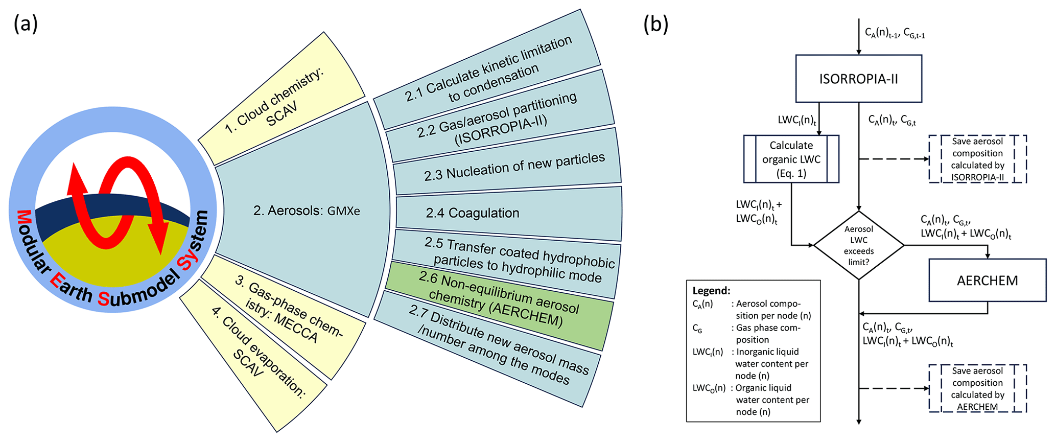
Figure 1 (a) Graphic summary of the calling sequence of chemical processes within MESSy (left) and the calling sequence of processes in the GMXe submodel (right). (b) Flow chart summarizing the data transfer between ISORROPIA-II and AERCHEM. Dashed attributes indicate the locations where the inorganic aerosol composition is saved as a separate output from ISORROPIA-II and AERCHEM used in the model evaluation presented in Sect. 4.

2.2 The Global Modal-aerosol eXtension (GMXe)

GMXe is used to calculate aerosol microphysics using seven modes to describe the log-normal size distributions; three hydrophobic modes that cover the size spectra of Aitken, accumulation, and coarse modes; and four hydrophilic modes that cover the same size range and additionally the size spectrum of nucleation. Each mode is defined in terms of total number concentration, particle mean radius, and geometric standard deviation of the radius distribution. Within each size mode, the aerosol composition is internally mixed (uniform) but varies between modes (externally mixed). Table 1 provides a summary of the recommended GMXe submodel setup for each mode when using AERCHEM.

Table 1 GMXe submodel setup used in this study. In GMXe, aerosol species are distributed between the four hydrophilic and three hydrophobic aerosol modes. Table adapted from Pringle et al. (2010).

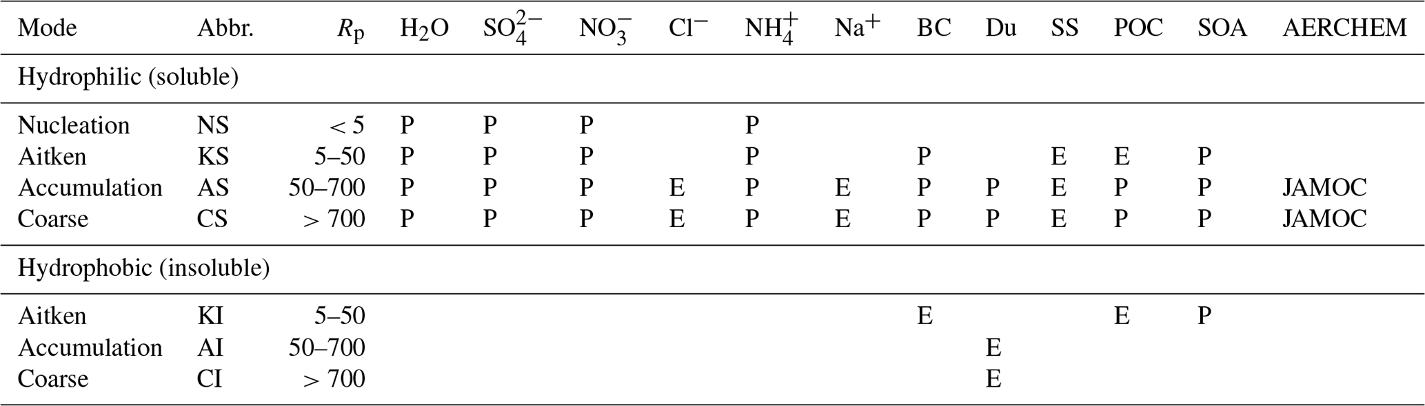
R_p refers to particle radius (nm), P indicates permitted in the mode, E indicates emitted into the mode, BC refers to black carbon, Du refers to dust, SS refers to sea spray, POC refers to primary organic carbon, and SOA refers to secondary organic aerosols.

ISORROPIA-II is used to calculate the thermodynamic equilibrium, which calculates the gas–liquid–solid equilibrium partitioning of K⁺–Ca²⁺–Mg²⁺–${\mathrm{NH}}_{\mathrm{4}}^{+}$–Na⁺–${\mathrm{SO}}_{\mathrm{4}}^{\mathrm{2}\mathrm{-}}$–${\mathrm{NO}}_{\mathrm{3}}^{\mathrm{-}}$–Cl⁻–H₂O aerosols. For this, it considers 19 salts in the solid phase and 15 aqueous-phase compounds. When using AERCHEM, it is assumed that all aerosols are in a metastable state, meaning that all aerosols have an aqueous phase which allows for supersaturation of dissolved salts. A detailed description of all processes represented in GMXe and ISORROPIA-II is provided by Pringle et al. (2010) and Fountoukis and Nenes (2007), respectively.

2.3 Aerosol water

The representation of non-equilibrium aerosol chemistry is inherently dependent on the aerosol liquid water content. In GMXe it is assumed that each particle mode is internally mixed, but ISORROPIA-II only considers the uptake of water by inorganic compounds (W_inorganic, g m⁻³). The aerosol water due to organic compounds, which is added to the aerosol water predicted by ISORROPIA-II, is calculated based on the mass concentration (m_s, g m⁻³) of all organics dissolved, the water (ρ_w, g m⁻³) and organic aerosol (ρ_s, g m⁻³) density, the relative humidity (RH, 0–1), and the hygroscopicity parameter (κ_organic) of the soluble organic:

$$\begin{array}{}\text{(1)}& W_{\mathrm{organic}}=m_s\cdot {\displaystyle \frac{{\mathit{\rho }}_{\mathrm{w}}}{{\mathit{\rho }}_s}}\cdot {\displaystyle \frac{{\mathit{\kappa }}_{\mathrm{organic}}}{\left(\frac{\mathrm{1}}{\mathrm{RH}}-\mathrm{1}\right)}}.\end{array}$$

The organic aerosol (OA) composition and evolution in the atmosphere are simulated within GMXe. Primary emitted organic aerosols are mainly emitted into the hydrophobic Aitken mode, with only a small fraction being assumed to be directly soluble and emitted into the hydrophilic Aitken mode. Here, an initial hygroscopicity parameter of 0.1 is assumed, as suggested by Lambe et al. (2011). GMXe represents the formation of secondary organic aerosols (SOAs) from isoprene, α-pinene, β-pinene, toluene, and xylene. For this, an additional SOA model was implemented into GMXe based on the two-product model originally proposed by Odum et al. (1996). This model has been described in detail elsewhere (Tsigaridis and Kanakidou, 2003; Zhang et al., 2007; O'Donnell et al., 2011), and a general description is presented in the Supplement of this paper. A summary of all hygroscopicity parameters used for each SOA species is provided in Table S2 in the Supplement.

2.4 Cloud–aerosol interactions

Similarly to gas-phase species, aerosols are directly influenced by scavenging processes, which are represented by the submodel SCAV in MESSy. First, SCAV computes the fraction of nucleation scavenging for each aerosol species. The scavenged fraction of each aerosol species is assumed to be instantly activated and represents the initial concentrations in cloud droplets used to compute in-cloud chemistry. Subsequently, SCAV calculates cloud chemical processes based on an aqueous-phase chemical mechanism selected by the user. While processing chemical processes in the aerosol and gas phase, it is assumed that the cloud composition remains constant and that all cloud tracers reside within cloud droplets. After GMXe and MECCA have calculated all aerosol processes and gas-phase chemistry, respectively, the cloud composition is considered to reside in the coarse mode if the cloud evaporates.

2.5 Additional aerosol removal processes

In addition to aerosol scavenging, the removal of aerosol tracers by dry deposition and sedimentation is considered by using MESSy's Dry DEPosition (DDEP) and SEDImentation (SEDI) submodels, respectively. From a technical point of view, dry deposition is only applied in the lowest model layer, whereas sedimentation occurs in the entire vertical column. In the case of aerosol particles, sedimentation is a significant sink, but it is no sink for trace gases. A detailed description of the technical representation in MESSy of both processes is presented by Kerkweg et al. (2006a).

3 The AERCHEM sub-submodel

3.1 Integration of AERCHEM in GMXe

AERCHEM is developed as an add-on to the thermodynamic equilibrium model (i.e. ISORROPIA-II) of GMXe. Similarly to MESSy, the sequence of simulated aerosol processes in GMXe is ordered by the processes' expected timescales within the atmosphere. The thermodynamic equilibrium is expected to be reached quickly, whereas the non-equilibrium aerosol chemistry is expected to act on longer timescales. Thus, AERCHEM is executed in series after the thermodynamic equilibrium calculations performed by ISORROPIA-II (see Fig. 1a). Figure 1b illustrates the data transfer between ISORROPIA-II and AERCHEM. Prior to performing the calculation by ISORROPIA-II, GMXe calculates the amount of each gas-phase species considered in ISORROPIA-II that is kinetically able to condense onto the aerosol (Fig. 1a, box 2.1) by assuming diffusion-limited condensation. This is achieved by extending the calculation for H₂SO₄ used in the M7 aerosol model presented by Vignati et al. (2004) for HNO₃, NH₃, and HCl. Afterward, the thermodynamic equilibrium is calculated using ISORROPIA-II. The aerosol concentrations per mode, as well as the total gas-phase concentrations, including the gas-phase fraction of each species that cannot condense onto the aerosol, are then transferred to AERCHEM. In AERCHEM, the total gas-phase concentration is considered since the diffusion limitation is directly included in the calculation of the phase transfer reactions performed; i.e. the Henry equilibrium is corrected by the kinetic diffusion limitation, which can become highly relevant in the case of further aqueous-phase reactions of the dissolved compounds. Before executing AERCHEM, the total aerosol liquid water content is calculated by adding the organic aerosol water (see Sect. 2.3) to the inorganic aerosol water calculated by ISORROPIA-II. The total aerosol liquid water content serves as the basis for all calculations performed by AERCHEM.

3.2 Representation of phase transfer

In AERCHEM, the exchange rate coefficients are calculated before the integration of the ODE system following Schwartz (1986). The forward ($k_{\mathrm{ex}}^{\mathrm{f}}$) exchange rates are based on the liquid water content (lwc, in m³(aq) m⁻³(air)), whereas the backward exchange rates ($k_{\mathrm{ex}}^{\mathrm{b}}$) are based on the Henry's law coefficient ($H_s^{\mathrm{cp}}$, in mol (m³ Pa)⁻¹), temperature (T, in K), and the universal gas constant (R, in J (mol K)⁻¹):

$$\begin{array}{}\text{(2)}& {\displaystyle }& {\displaystyle }{k}_{\mathrm{ex}}^{\mathrm{f}}=k_{\mathrm{mt}}\cdot \mathrm{lwc},\text{(3)}& {\displaystyle }& {\displaystyle }{k}_{\mathrm{ex}}^{\mathrm{b}}=k_{\mathrm{mt}}\cdot {\left(H_s^{\mathrm{cp}}\cdot R\cdot T\right)}^{-\mathrm{1}}.\end{array}$$

Here, k_mt denotes the mass transfer coefficient of the given species. The mass transfer coefficient is limited by gas-phase diffusion (D_g, in m² s⁻¹) and is calculated for a single aerosol as follows:

$$\begin{array}{}\text{(4)}& k_{\mathrm{mt}}={\left({\displaystyle \frac{r^{\mathrm{2}}}{\mathrm{3}{D}_{\mathrm{g}}}}+{\displaystyle \frac{\mathrm{4}r}{\mathrm{3}\stackrel{\mathrm{‾}}{v}\mathit{\alpha }}}\right)}^{-\mathrm{1}},\end{array}$$

where r represents the particle radius (in m), α represents the accommodation coefficient of the given species, and $\stackrel{\mathrm{‾}}{v}$ (in m s⁻¹) represents the mean molecular velocity from the Boltzmann velocity distribution.

3.3 Aqueous-phase mechanisms for AERCHEM

In AERCHEM, dissociation, hydration, and oxidation reaction rates are taken from the literature. The photolysis reaction rates are calculated outside AERCHEM and are provided by the MESSy submodel JVAL (Sander et al., 2014). So far, all kinetic mechanisms used in MESSy submodels are built via the Kinetic PreProcessor (KPP; Sandu and Sander, 2006). To simplify the usage and enhance the consistency between all mechanisms used for the different phases (gas phase – MECCA, aqueous phase – SCAV, aerosol phase – GMXe–AERCHEM), the full mechanism is hosted within the MECCA submodel. Before compiling the MESSy code, the user is able to choose the required mechanisms. The supplementary material of this paper includes a manual for AERCHEM, outlining the procedure of selecting the desired mechanism. The following list provides a short overview of the tailor-made aqueous-phase mechanisms currently available for AERCHEM, sorted by their complexity:

• The simplest aqueous-phase mechanism considers a few soluble compounds, their acid–base equilibria, and the oxidation of SO₂ by O₃ and H₂O₂ (abbreviated as Scm; Jöckel et al., 2006).

• A more complex aqueous-phase mechanism represents more than 150 reactions (abbreviated as Sc; Tost et al., 2007). It includes aqueous-phase HO_x chemistry and the destruction of O₃ by ${\mathrm{O}}_{\mathrm{2}}^{-}$, but it is missing a detailed representation of aqueous-phase oxidation of oxygenated volatile organic compounds (OVOCs). This mechanism can be considered to be the current standard mechanism for representing cloud chemical processes in MESSy (Jöckel et al., 2016).

• The most complex aqueous-phase mechanism is the recently developed Jülich Aqueous-phase Mechanism of Organic Chemistry (abbreviated as JAMOC; Rosanka et al., 2021c, b, a). JAMOC includes a complex aqueous-phase OVOC oxidation scheme and represents the phase transfer of species containing up to 10 carbon atoms and the oxidation of species containing up to 4 carbon atoms. The photo-oxidation of species with three or four carbon atoms is limited to the major isoprene oxidation products (i.e. methylglyoxal, methacrolein, and methyl vinyl ketone) and the aqueous-phase sources of methylglyoxal. Overall, JAMOC represents the phase transfer of 350 species, 43 equilibria (acid–base and hydration), and more than 280 photo-oxidation reactions. A detailed description of JAMOC is presented by Rosanka et al. (2021c). When using JAMOC, the user needs to select the Mainz Organic Mechanism (MOM) to represent gas-phase chemistry in MECCA.

A detailed comparison of all three mechanisms is provided by Rosanka et al. (2021b, their Table 1). All reaction rates, Henry's law, accommodation coefficients, and other model parameters are provided by Rosanka et al. (2021c) and Sander (2021).

3.4 Solving the ODE system and numerical challenges

In order to numerically integrate the aqueous-phase chemical reaction mechanism, AERCHEM uses KPP. When using the KPP software, the user may choose between several numerical solvers. For numerically complex multiphase chemistry problems, Rosenbrock solvers are known to be some of the most efficient solvers. Due to its favourable performance, the Rodas-3 (Sandu et al., 1997) Rosenbrock integrator, with automatic time step control, is selected as the default integrator in AERCHEM. We find that Rodas-3 provides the best combination of efficiency and stability when using relative and absolute tolerances of $\mathrm{1}\times {\mathrm{10}}^{-\mathrm{3}}$ and 1 molec. cm⁻³, respectively.

Due to the phase transfer reactions and equilibria, the stiffness of the ODE system increases with decreasing aerosol liquid water content. For this reason, AERCHEM performs the chemistry calculations only in the two larger hydrophilic (accumulation and coarse) modes in series. The accumulation mode is calculated first, conforming to the order utilized for ISORROPIA-II. In order to ensure a proper stability of the numerical solver, AERCHEM is only executed if the aerosol liquid water content exceeds $\mathrm{1}\times {\mathrm{10}}^{-\mathrm{14}}$ m³(aq) m⁻³(air) (see Fig. 1b). This low limit is 2 orders of magnitude lower than an earlier attempt to represent non-equilibrium aerosol chemistry on global scales by Kerkweg et al. (2007), who did not use operator splitting of the gas- and aqueous-phase chemistry. In their study, the non-equilibrium aerosol chemistry was almost exclusively executed in the marine boundary layer. With the limit used in AERCHEM, calculations of non-equilibrium aerosol chemistry are available over continental regions.

4 Example results using AERCHEM

The primary objective of this section is to showcase initial findings obtained by using AERCHEM in GMXe within MESSy. Here, the fifth-generation European Centre Hamburg general circulation model (ECHAM5, version 5.3.02; Roeckner et al., 2003) is used as the core atmospheric model. This combination is known as the ECHAM/MESSy Atmospheric Chemistry (EMAC) model. The physics subroutines of the original ECHAM code have been modularized and re-implemented as MESSy submodels and have continuously been further developed. Only the spectral transform core, the flux-form semi-Lagrangian large-scale advection scheme, and the nudging routines for Newtonian relaxation remain from ECHAM. Our focus lies in determining whether AERCHEM adequately represents background concentrations rather than episodic events. As such, we restrict our comparisons to long-term observational datasets containing numerous observations at multiple sites and exclude single measurement campaigns that are limited with regard to spatial and temporal representativeness. Examining the latter would require detailed process studies for specific conditions, which is beyond the scope of this study. For the comparison, we primarily emphasize inorganic aerosol mass concentrations, which are frequently observed.

4.1 EMAC modelling setup

In order to keep the computational demand low, we evaluate the implication of AERCHEM by applying EMAC at a resolution of T42L31, i.e. with a spherical truncation of T42 (corresponding to a quadratic Gaussian grid of approximately 2.8° × 2.8° in latitude and longitude) with 31 vertical hybrid pressure levels up to 10 hPa, of which about 22 levels represent the troposphere. Here, we use the standard time step length for this resolution of 900 s. In order to reproduce the actual day-to-day meteorology in the troposphere, the dynamics have been weakly nudged (Jöckel et al., 2006) towards the ERA-Interim (Dee et al., 2011) reanalysis data of the European Centre for Medium-Range Weather Forecasts (ECMWF).

Atmospheric gas-phase chemistry is represented in MECCA using the Mainz Organic Mechanism (MOM) recently evaluated by Pozzer et al. (2022). MOM contains an extensive oxidation scheme for isoprene (Taraborrelli et al., 2009, 2012; Nölscher et al., 2014; Novelli et al., 2020), monoterpenes (Hens et al., 2014), and aromatics (Cabrera-Perez et al., 2016; Taraborrelli et al., 2021). In addition, comprehensive reaction schemes are considered for the modelling of the chemistry of NO_x, HO_x, CH₄, and anthropogenic linear hydrocarbons. VOCs are oxidized by OH, O₃, and NO₃, whereas RO₂ reacts with HO₂, NO_x, and NO₃ and undergoes self- and cross-reactions. All in all, MOM considers 43 primarily emitted VOCs and represents more than 600 species and 1600 reactions (Sander et al., 2019). In order to push EMAC to its technical limits, we represent the aqueous-phase chemistry in cloud droplets, rain (i.e. by using SCAV), and deliquescent aerosols (i.e. by using AERCHEM) using JAMOC (see Sect. 3.3).

Anthropogenic emissions are based on the Emissions Database for Global Atmospheric Research (EDGAR, v4.3.2; Crippa et al., 2018) and are vertically distributed following Pozzer et al. (2009). The Model of Emissions of Gases and Aerosols from Nature (MEGAN; Guenther et al., 2006) is used to calculate biogenic VOC emissions. Biomass burning emission fluxes are calculated using the MESSy submodel BIOBURN, which calculates these fluxes based on biomass burning emission factors and dry-matter combustion rates. For the latter, Global Fire Assimilation System (GFAS) data are used, which are based on satellite observations of fire radiative power from the Moderate Resolution Imaging Spectroradiometer (MODIS) satellite instruments (Kaiser et al., 2012). GMXe considers the emission of SO₂ from anthropogenic activities (EDGAR, v4.3.2), biomass burning (BIOBURN), and volcanic activities based on the AEROCOM dataset (Dentener et al., 2006). For primary organic aerosol (POA) and black carbon (BC) emissions, GMXe considered anthropogenic emissions in the lower troposphere and from aviation activities (EDGAR, v4.3.2) and biomass burning (BIOBURN). Mineral dust emissions are calculated online following Astitha et al. (2012) and are represented as bulk inert dust; i.e. no crustal elements are emitted. Sea spray aerosol emissions are calculated online following Kerkweg et al. (2006b), assuming the chemical composition proposed by Seinfeld and Pandis (2016, their Table 8.8). A summary of all emissions considered in GMXe, including all related scaling factors, is provided in the Fortran Namelist S1.

Within this study, we perform one simulation for 2010 using 2009 as the spin-up. This simulation was performed at the Jülich Supercomputing Centre using the Jülich Wizard for European Leadership Science (JUWELS) cluster (Jülich Supercomputing Centre, 2019).

4.2 Inorganic aerosol composition

In the following, EMAC-simulated aerosol masses using AERCHEM for sulfate (${\mathrm{SO}}_{\mathrm{4}}^{\mathrm{2}-}$), nitrate (${\mathrm{NO}}_{\mathrm{3}}^{-}$), ammonium (${\mathrm{NH}}_{\mathrm{4}}^{+}$), and chloride (Cl⁻) are evaluated. We compare annual and seasonal mean concentrations to three in situ monitoring networks: (1) for the United States we rely on the Clean Air Status and Trends Network (CASTNET) operated by the Clean Air Markets Division of the US Environmental Protection Agency (EPA), which provides weekly filter pack observations; (2) for Europe we use the co-operative programme for monitoring and evaluation of the long-range transmission of air pollutants in Europe (EMEP); and (3) for East Asia we use the Acid Deposition Monitoring Network in East Asia (EANET). Observed concentrations are interpolated onto the EMAC grid. If multiple stations coincide with the same model grid box, the average of all these stations is used for the comparison. In addition, the aerosol compositions simulated by ISORROPIA-II and AERCHEM are compared at each observational site. Both compositions are obtained from the same EMAC simulation by providing the mass concentration of each species simulated by ISORROPIA-II (which is used as an AERCHEM input) and by AERCHEM as separate model outputs. The exact location where both compositional data are obtained in GMXe is summarized in Fig. 1b. Figure S1 provides box plots presenting the observations with the simulated concentrations by ISORROPIA-II and AERCHEM for each inorganic species and observation network.

4.2.1 Sulfate (${\mathrm{SO}}_{\mathrm{4}}^{\mathrm{2}-}$)

Figure 2a shows the annual surface mean sulfate (${\mathrm{SO}}_{\mathrm{4}}^{\mathrm{2}-}$) concentration simulated by EMAC using AERCHEM and that observed at the three monitoring networks in 2010. Overall, the model reproduces the observed concentrations well. In the United States, the model nicely captures the east–west and the north–south gradients in the sulfate EPA observations. The simulated sulfate concentrations for almost all EPA stations are within a factor of 2 of the observed values (Fig. 2b). Only for two station does EMAC using AERCHEM predict values that are slightly higher than a factor of 2.

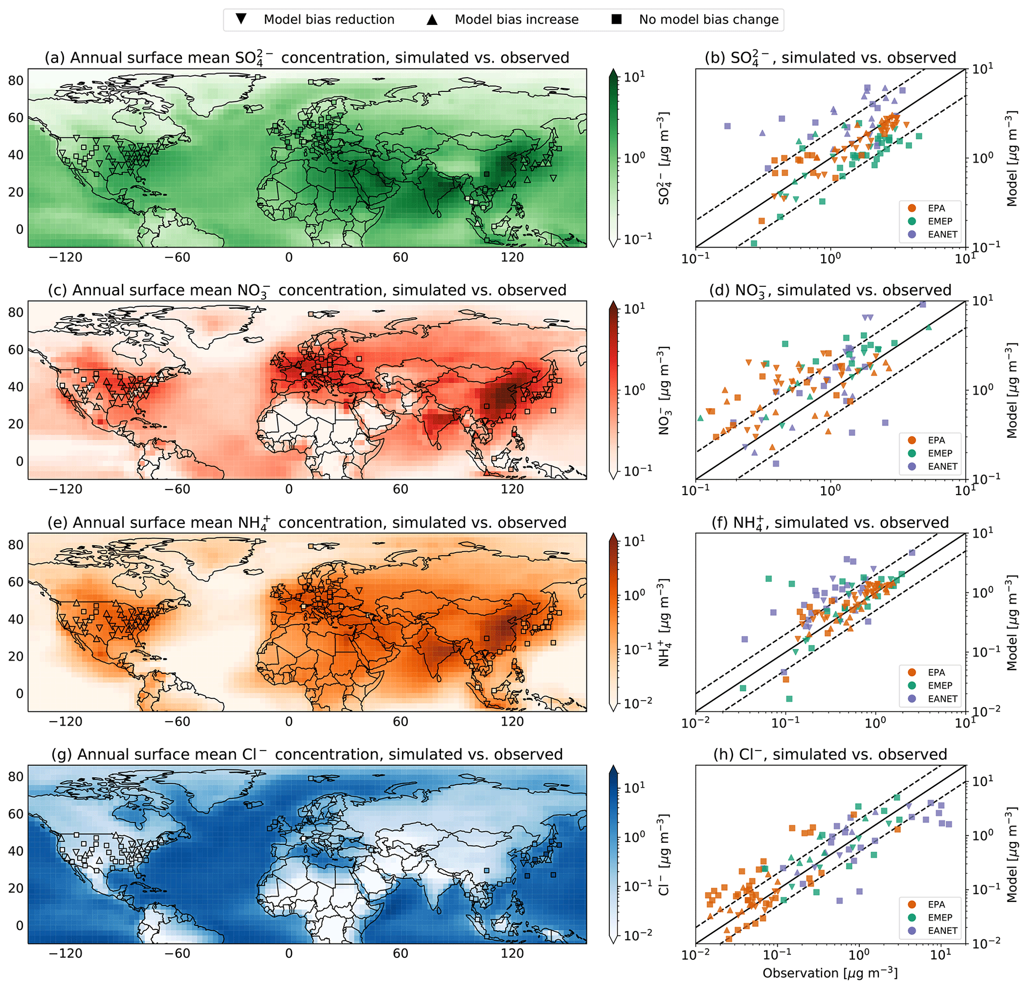
Figure 2 Annual surface mean for (a) sulfate (${\mathrm{SO}}_{\mathrm{4}}^{\mathrm{2}-}$), (c) nitrate (${\mathrm{NO}}_{\mathrm{3}}^{-}$), (e) ammonium (${\mathrm{NH}}_{\mathrm{4}}^{+}$), and (g) chloride (Cl⁻) concentrations simulated by EMAC using AERCHEM for the year 2010. Annual surface mean observational concentration for stations in the EPA (USA), EMEP (Europe), and EANET (East Asia) networks are depicted as triangles and boxes. A triangle pointing down indicates a model bias reduction when using AERCHEM compared to ISORROPIA-II, whereas a triangle pointing up indicates a model bias increase. Boxes indicate stations for which the simulated annual mean difference between AERCHEM and ISORROPIA-II does not exceed 5 %. Panels (b), (d), (f), and (h) show the direct comparison between model-simulated values and observations from EPA, EMEP, and EANET for sulfate, nitrate, ammonium, and chloride concentrations, respectively.

For an overwhelming number of EPA stations in the eastern US, the consideration of AERCHEM reduces EMAC's bias in predicting sulfate compared to simulated values by ISORROPIA-II (indicated by downward-pointing triangles in Fig. 2). An insignificant difference between simulated values of ISORROPIA-II and AERCHEM is observed in the Midwest. Figure 3 shows so-called Taylor diagrams (Taylor, 2001) used to evaluate the statistical performance improvements for multiple models. In order to allow for a comparison between all observation networks and each season (DJF – December, January, February; MAM – March, April, May; JJA – June, July, August; and SON – September, October, November), we normalized the standard deviation by the observed standard deviation. Overall, the annual mean model bias for the EPA network is more than halved by AERCHEM, changing from −0.33 to −0.14 µg m⁻³. At the same time, the normalized standard deviation improves from 0.83 to 0.96. Both statistical measures improve in DJF, MAM, and JJA, with the most substantial change modelled in JJA. Here, the usage of AERCHEM reduces the mean model bias from −0.79 to −0.37 µg m⁻³, and the normalized standard deviation improves from 0.62 to 0.80. However, in SON both the mean model bias and normalized standard deviation worsen to 0.58 µg m⁻³ (from 0.47 µg m⁻³) and 1.60 (from 1.47), respectively. Further reductions in the model bias and normalized standard deviation are expected by accounting for the reactive uptake of IEPOX from isoprene, which produces stable organosulfates (Eddingsaas et al., 2010; Wieser et al., 2023). A similar good agreement is observed in Europe, where the east–west gradient is also nicely matched, even though EMAC tends to be biased low, especially in continental eastern Europe. Compared to the EPA network, the statistical improvement is less pronounced when using AERCHEM, with a slight improvement in the annual mean model bias from −0.82 to −0.77 µg m⁻³ and a minor improvement in the normalized standard deviation to 0.27 (from 0.24). Similar improvements in the mean model bias are observed for all seasons. Overall, the model agrees reasonably well in Japan, South Korea, Russia and China, but it tends to be biased low. Even though the annual mean model bias is significantly reduced from −0.40 to −0.09 µg m⁻³, the normalized standard deviation only increases slightly from 0.42 to 0.48. In Southeast Asia, especially in Myanmar, Thailand, and Kuala Lumpur in Malaysia, the model tends to significantly overpredict sulfate concentrations. In JJA and SON, the normalized standard deviation improves slightly, but the correlation of AERCHEM to the observations worsens. Especially during these seasons, these regions are highly photochemically active, where chemical sulfate losses might be of importance, as has been recently described by Pan et al. (2019), Ren et al. (2021), Liu et al. (2021), and Cope et al. (2022). With the development of AERCHEM, all these processes can now be explicitly represented in EMAC, potentially reducing the observed model biases.

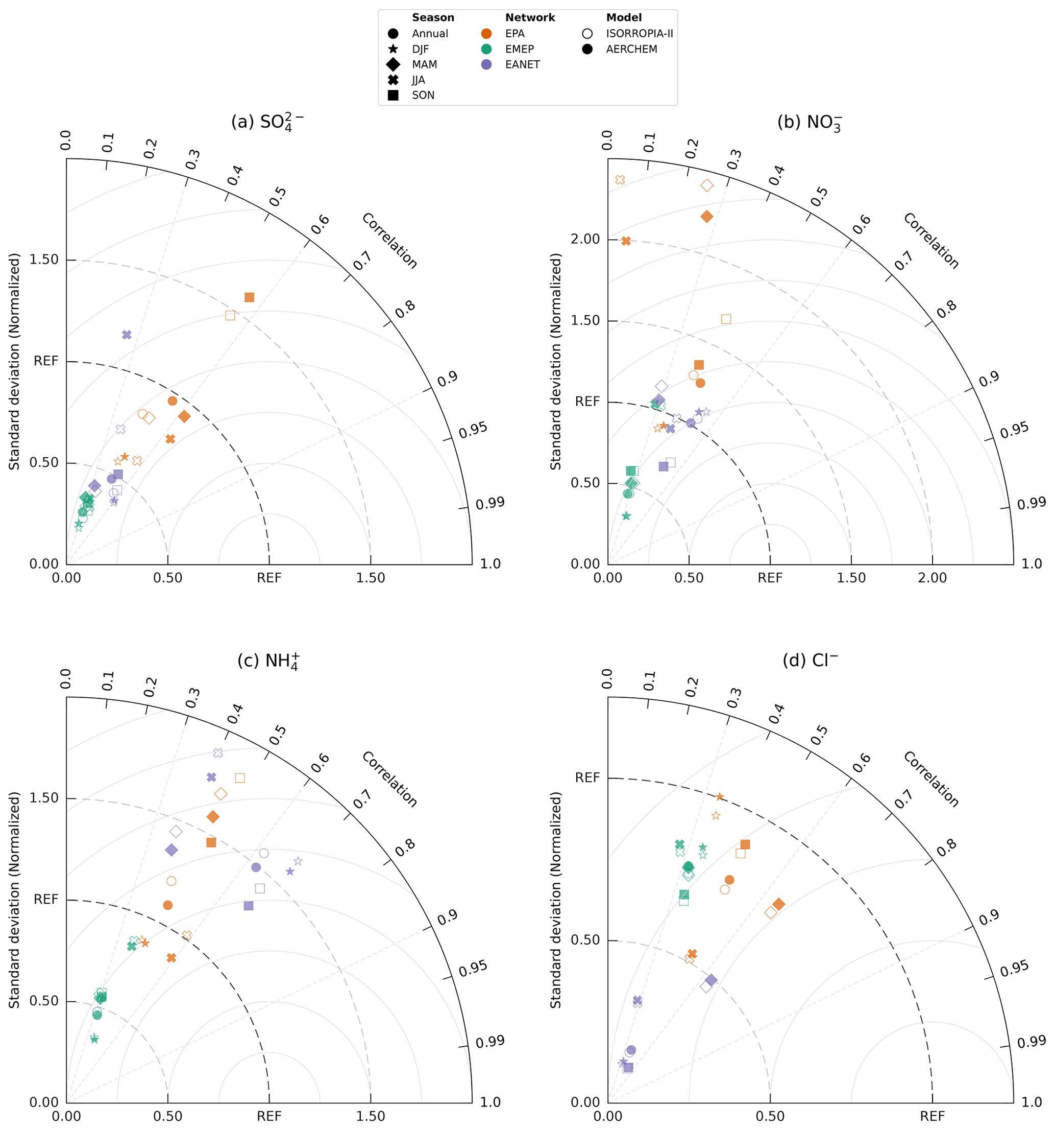
Figure 3 Taylor diagrams for (a) sulfate (${\mathrm{SO}}_{\mathrm{4}}^{\mathrm{2}-}$), (b) nitrate (${\mathrm{NO}}_{\mathrm{3}}^{-}$), (c) ammonium (${\mathrm{NH}}_{\mathrm{4}}^{+}$), and (d) chloride (Cl⁻) for each season, observation network (EPA, EMEP, and EANET), and model (ISORROPIA-II and AERCHEM). The standard deviation is normalized by the observed standard deviation.

4.2.2 Nitrate (${\mathrm{NO}}_{\mathrm{3}}^{-}$)

The annual mean nitrate (${\mathrm{NO}}_{\mathrm{3}}^{-}$) concentrations simulated by EMAC using AERCHEM and observed at the EPA, EMEP, and EANET stations are shown in Fig. 2c. In the continental US, EMAC simulates the spatial pattern observed by the EPA network reasonably well. Large nitrate concentrations are simulated within a factor of 2 (Fig. 2d), but the model tends to overpredict low nitrate concentrations in the Midwest and northeastern states. However, compared to the nitrate concentrations simulated by ISORROPIA-II, AERCHEM reduces EMAC's bias in simulated nitrate concentrations (Fig. 3b). The annual mean model bias improves from 0.63 to 0.49 µg m⁻³, and the normalized standard deviation improves from 1.28 to 1.25 when using AERCHEM. Similarly to the US, EMAC is biased high in continental Europe, but the number of stations in Europe for which AERCHEM predicts nitrate concentrations that are higher than a factor of 2 compared to observations from EMEP is lower. The spatial variability with higher concentrations in central Europe and with lower concentrations in northern Europe is reasonably matched. EMAC tends to reproduce nitrate hotspots in the Benelux countries and nitrate concentrations in Ireland. There is one significant outlier in Switzerland, where EMAC predicts significantly higher nitrate concentrations than observed. This station is located on the Jungfraujoch at about 3570 m. Due to the coarse model resolution used, EMAC is not capable to resolve the high elevation of this station properly, leading to significantly higher simulated values. Interestingly, the mean model bias only improves during the winter months (DJF) from −0.12 to −0.07 µg m⁻³, whereas, for all other seasons and thus the annual comparison, the mean model bias worsens when using AERCHEM. It is important to keep in mind that nitrate concentrations reported by EMEP are mainly based on Teflon filters and are thus potentially systematically underestimated (Ames and Malm, 2001). In general, the spatial distribution of nitrate concentrations in Southeast Asia (e.g. Myanmar, Thailand, Vietnam, Cambodia, Malaysia, Indonesia) are properly simulated, and nitrate hotspots in East Asia, like in central China or Jakarta, are reproduced reasonably well by EMAC. In Japan and South Korea, nitrate is slightly overestimated, but the usage of AERCHEM reduces EMAC's bias. In the remote marine boundary layer (i.e. on Okinawa and on the Ogasawara Islands) EMAC tends to slightly overpredict nitrate concentrations. The improvements provided by AERCHEM may stem from the reaction of nitrate anion with the ${\mathrm{SO}}_{\mathrm{4}}^{\mathrm{2}-}$, leading to nitrate radicals which either outgas or photolyse efficiently. However, across all EANET stations, the usage of AERCHEM slightly increases the mean model bias in all seasons, but the normalized standard deviation is improved for the annual comparison (from 1.06 to an ideal 1.00), as well as in DJF and MAM. Nevertheless, a much larger reduction in the model overpredictions is expected as a result of including the known chemistry of reactive nitrogen, essentially mediating NO_x recycling via production of HONO (Ye et al., 2017; Andersen et al., 2023) and ClNO₂ (Thornton et al., 2010), which is currently not included in JAMOC. The role of particulate organic nitrate for predictions of inorganic nitrate is yet to be assessed. Many organic nitrates are known to hydrolyze (Liu et al., 2012; Boyd et al., 2015; Vasquez et al., 2020), not always leading to a release of ${\mathrm{NO}}_{\mathrm{3}}^{-}$ (Zare et al., 2019). Even though these processes are currently not included in JAMOC, a global analysis of the importance of organic nitrate hydrolysis reactions can be easily realized due to the flexible design of AERCHEM.

4.2.3 Ammonium (${\mathrm{NH}}_{\mathrm{4}}^{+}$)

In the eastern US, EMAC matches the EPA observations reasonably well overall but overestimates ammonium concentrations in the Midwest for both ISORROPIA-II and AERCHEM (see Fig. 2e). For only four stations, the simulated difference in the concentration is slightly higher than a factor of 2. Even though EMAC is capable of representing the east–west gradient in the US, due to the slight overestimation in the Midwest, the simulated east–west gradient is too low. The consideration of non-equilibrium aqueous-phase chemistry in aerosols leads to a reduced model bias for most EPA stations. The annual mean model bias (Fig. 3c) is reduced from 0.19 to 0.11 µg m⁻³, whereas the normalized standard deviation is reduced by 0.11 to 1.09. The strongest model bias reduction occurs in autumn (SON), decreasing to 0.29 µg m⁻³ (from 0.45 µg m⁻³), but the normalized standard deviation worsens. Over the contiguous US, the highest ammonia (NH₃) concentrations are observed in spring (MAM) and summer (JJA) (Wang et al., 2021). In spring, AERCHEM improves the statistical comparison between EMAC and the observations, with a reduction in the mean model bias of 0.06 µg m⁻³ and a reduction in the normalized standard deviation of 0.12, whereas the mean model bias worsens in summer by 0.08 µg m⁻³, with a worsening in the normalized standard deviation. Ammonium concentrations in central Europe are reproduced reasonably well, and almost all simulated values are within a factor of 2. EMAC again fails to reproduce low ammonium concentrations, as observed at the Jungfraujoch (see discussion above). For this station, the lowest value in continental Europe is observed. Again, EMAC is capable of reproducing the north–south gradient in Europe, but it underestimates its amplitude and thus systematically overestimates concentrations in northern Europe. In Europe, statistical improvements when using AERCHEM are minor (Fig. 3c). In East Asia, EMAC systematically overpredicts ammonium concentrations in continental regions, Japan, and the remote marine boundary layer but manages to reproduce ammonium hotspots (e.g. central China, central Java) reasonably well. Across all seasons, the mean model bias and the normalized standard deviation are systematically reduced when using AERCHEM. The overall annual mean model bias is reduced by 0.06 to 0.35 µg m⁻³, and the annual normalized standard deviation is reduced from 1.60 to 1.49. At the moment, JAMOC only represents the uptake of ammonia and its protonation. Thus, the changes in ammonium are potentially mainly related to the changes in sulfate and nitrate. A proper budget analysis similar to the methodology presented by Gromov et al. (2010) is thus warranted in the future.

4.2.4 Chloride (Cl⁻)

Over the central US, EMAC using AERCHEM tends to overestimate chloride (Cl⁻) concentrations (Fig. 2g). EMAC reproduces chloride concentrations in coastal regions (e.g. Florida, San Francisco), which are frequently influenced by sea salt emissions. Similarly, observations in Ireland, Iceland, coastal regions in the Benelux countries, and coastal regions in northern Europe are well captured by EMAC. High chloride concentrations in coastal regions in East Asia are also well reproduced, especially in the remote marine boundary layer (i.e. on Okinawa and on the Ogasawara Islands). At a few observational stations in southern Japan, EMAC tends to slightly underestimate very high chloride concentrations. Overall, differences in simulated concentrations from AERCHEM and ISORROPIA-II at in situ measurement stations are minor. Similarly, the changes between ISORROPIA-II and AERCHEM in the mean model bias are minor for all networks (Fig. 3d). In the US and Europe, the annual mean model bias worsens by about 15 %. In Asia, the annual mean model bias improves from −2.19 to −2.12 µg m⁻³. For all networks, using AERCHEM improves the normalized standard deviation for all seasons. In AERCHEM, chloride is not inert and undergoes oxidation by hydroxyl radicals triggering the production of HCl, HOCl, and Cl₂. The latter two are relatively insoluble and efficiently transfer chlorine to the gas phase. Missing reactions following N₂O₅ uptake (Soni et al., 2023) and ${\mathrm{NO}}_{\mathrm{3}}^{-}$ photolysis (Dalton et al., 2023) are likely to have a larger impact.

4.3 Aerosol acidity

4.3.1 Aerosol acidity calculations

The aerosol pH is defined as the negative decimal logarithm of the hydrogen ion activity ($a_{{\mathrm{H}}^{+}}$):

$$\begin{array}{}\text{(5)}& \mathrm{pH}=-{\log }_{\mathrm{10}}\left(a_{{\mathrm{H}}^{+}}\right),\end{array}$$

where the hydrogen activity can be calculated by multiplying the hydrogen ion activity coefficient (${\mathit{\gamma }}_{{\mathrm{H}}^{+}}$) and the hydrogen ion molarity ($x_{{\mathrm{H}}^{+}}$, in mol L⁻¹). In order to account for the differences induced by the non-equilibrium aerosol chemistry, we calculate the aerosol pH for fine particles (PM_2.5, diameter <2.5 µm) in order to allow for direct comparisons with observational data. For this, the hydrogen ion molarity is estimated by the following:

$$\begin{array}{}\text{(6)}& x_{{\mathrm{H}}_{{\mathrm{PM}}_{\mathrm{2.5}}}^{+}}={\displaystyle \frac{\sum [{\mathrm{H}}^{+}{]}_{\mathrm{i}}\cdot f_{{\mathrm{PM}}_{{\mathrm{2.5}}_{\mathrm{i}}}}}{\sum [{\mathrm{H}}_{\mathrm{2}}\mathrm{O}{]}_{\mathrm{i}}\cdot f_{{\mathrm{PM}}_{{\mathrm{2.5}}_{\mathrm{i}}}}}}\cdot {\mathit{\rho }}_{{\mathrm{H}}_{\mathrm{2}}\mathrm{O}}={\displaystyle \frac{[{\mathrm{H}}^{+}{]}_{{\mathrm{PM}}_{\mathrm{2.5}}}}{[{\mathrm{H}}_{\mathrm{2}}\mathrm{O}{]}_{{\mathrm{PM}}_{\mathrm{2.5}}}}}\cdot {\mathit{\rho }}_{{\mathrm{H}}_{\mathrm{2}}\mathrm{O}},\end{array}$$

where ${\mathit{\rho }}_{{\mathrm{H}}_{\mathrm{2}}\mathrm{O}}$ is the water density (g L⁻¹), and [H⁺]_i and [H₂O]_i are the hydrogen ion mass concentration (µg m⁻³ ≡ µmol m⁻³) and water mass concentration (µg m⁻³) of the hydrophilic mode i, respectively. $f_{{\mathrm{PM}}_{{\mathrm{2.5}}_{\mathrm{i}}}}$ represents the volume fraction of the given hydrophilic aerosol mode contained in fine particles with a diameter below 2.5 µm. The pH calculations are carried out exclusively when an adequate amount of water exists within the aerosol (total PM_2.5 water exceeds 0.01 µg m⁻³). For the pH calculations for ISORROPIA-II and AERCHEM, we assume that the hydrogen ion activity coefficient is 1. All pH calculation are performed based on instantaneous output provided every 5 h.

4.3.2 Simulated aerosol acidity

Figure 4a and b show the annual mean aerosol pH of fine particles (PM_2.5, diameter <2.5 µm) based on the H⁺ concentration simulated by ISORROPIA-II and AERCHEM, respectively. Separate model outputs for the H⁺ concentration are provided after the calculation performed by ISORROPIA-II and AERCHEM for the same EMAC simulation. In both cases, the aerosol liquid water content is calculated following Sect. 2.3. Here, the annual mean fine-aerosol pH based on n, the number of 5-hourly model outputs per year, is calculated as follows:

$$\begin{array}{}\text{(7)}& \stackrel{\mathrm{‾}}{{\text{pH}}_{{\mathrm{PM}}_{\mathrm{2.5}}}}={\displaystyle \frac{\mathrm{1}}{n}}\sum _{i=\mathrm{1}}^n-{\log }_{\mathrm{10}}\left(a_{{{\mathrm{H}}^{+}}_{{\mathrm{PM}}_{{\mathrm{2.5}}_{\mathrm{i}}}}}\right).\end{array}$$

When non-equilibrium aerosol chemistry is not taken into account (i.e. simulated values from ISORROPIA-II), EMAC predicts predominantly alkaline fine particles over the ocean. Further, mostly acid particles are simulated over continental regions influenced by anthropogenic activities. For continental regions in the Northern Hemisphere above 60° N and Australia, AERCHEM predicts slightly higher aerosol acidity. Differences in aerosol acidity simulated by AERCHEM compared to ISORROPIA-II in central Europe and the southeastern US are only minor. In some polluted continental regions (e.g. China, Southeast Asia, central Africa, Mexico, central South America), on the other hand, the usage of AERCHEM results in slightly higher aerosol pH compared to ISORROPIA-II predictions. Interestingly, for the accumulation mode, AERCHEM simulates a higher acidity over continental regions (see Fig. S2) but tends to simulate slightly higher pH for the coarse mode (see Fig. S3). This suggests that, even though the coarse mode (particles diameter >1.4 µm) only contributes minor fractions to the fine-aerosol acidity, changes in the fine-aerosol pH are driven by coarse-mode compositional changes. In addition, AERCHEM predicts slightly more alkaline fine particles over major deserts (e.g. Sahara, Lut Desert, Thar Desert, and Arabian Desert). The most substantial differences in aerosol acidity are simulated for fine particles in the marine boundary layer. Exclusively higher fine-aerosol acidity is simulated over all major oceans. At the same time, a high variability in differences between values simulated by AERCHEM and ISORROPIA-II is observed. The highest differences are simulated over the Southern Ocean, central Atlantic Ocean, and central Pacific Ocean. Lower differences are simulated over the Indian Ocean, the northern and southern Atlantic, and the southern Pacific and in the northern Pacific just west of the US. Sea salt aerosol particles are mainly emitted into the coarse mode. ISORROPIA-II simulates these aerosols to be alkaline (see Fig. S3), whereas AERCHEM suggests a higher acidity. Acidification of sea salt aerosols is partly due to the relatively fast oxidation of chloride by hydroxyl radicals, which eventually leads to hydrochloric acid formation. Moreover, methanesulfonic acid from DMS oxidation is a strong acid and contributes to lowering the pH. As expected, this effect is more pronounced over photochemically active regions with high sea salt and/or DMS emissions.

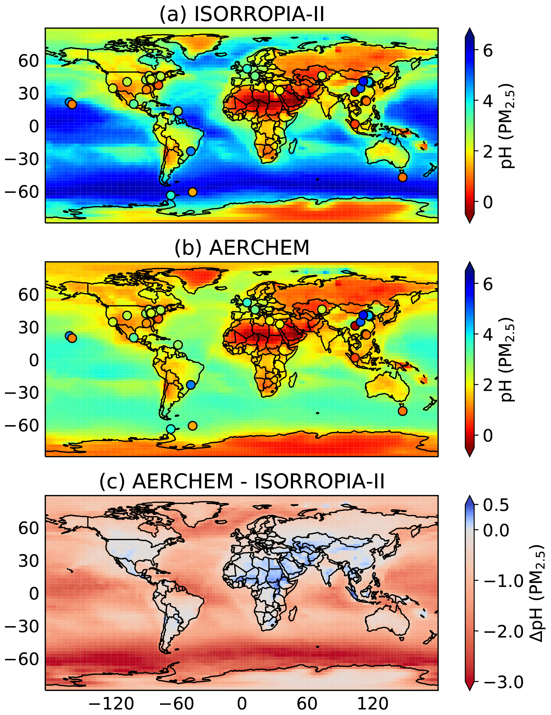
Figure 4 Mean annual aerosol pH for fine particles (PM_2.5, diameter <2.5 µm) simulated by (a) ISORROPIA-II and by (b) AERCHEM. Subfigure (c) represents the absolute difference of the annual means. In both cases, the aerosol liquid water content is calculated following Sect. 2.3. Section 4.3.1 elaborates on how the aerosol pH for fine particles is calculated based on the four hydrophilic lognormal modes. The annual mean is calculated following Eq. (7). Please note that, for the figure showing the absolute pH differences, an increase in acidity (decrease in pH) is indicated by red shading, whereas an increase in pH is indicated in blue. For comparison, observed fine-particle acidity, based on the dataset published by Pye (2020), is indicated by circles in panels (a) and (b).

4.3.3 Comparison to observational datasets

Evaluating the pH agreement with observations of an atmospheric chemistry model is difficult since no direct measurements of aerosol acidity are available and since observed aerosol acidities are estimated using thermodynamic equilibrium models (e.g. ISORROPIA-II). Assumptions made when using these models, ranging from the species that are considered (e.g. crustal species) to stable vs. metastable assumptions to averaging over certain time periods, can significantly affect the predicted aerosol pH. In addition, the spatial variability is limited and mostly bound to continental regions in the Northern Hemisphere. Still, in order to represent the spatial variability of aerosol acidity simulated by EMAC, we include pH values for fine aerosols derived from observations compiled by Pye et al. (2020) in Fig. 4a and b. However, please keep in mind that, due to the large uncertainties in observed aerosol acidity, these values are not intended to evaluate the model at a specific location. Overall, both ISORROPIA-II and AERCHEM reasonably reproduce aerosol acidity in the USA, Europe, Mexico, and Southeast Asia. In northern Asia, very high aerosol pH values are observed, which both AERCHEM and ISORROPIA-II fail to reproduce. The mean fine-aerosol pH across all continental observation locations is 2.7, where both ISORROPIA-II and AERCHEM predict a mean fine-aerosol pH of 1.8. By predicting a higher acidity for fine aerosols in the marine boundary layer, EMAC's predictions skills seem to improve when using AERCHEM. This is especially true for observations made at the Guiana Basin, in the Southern Ocean north of Antarctica, where the largest difference in pH is simulated, and for observations south of Australia. The mean fine-aerosol pH of 2.5 across all marine boundary observations predicted by AERCHEM gets closer to the observational mean of 2.1, whereas ISORROPIA-II predicts a mean value of 3.9. The higher aerosol acidity in the marine boundary layer is in line with a recent measurement study by Angle et al. (2021), suggesting a fast acidification of sea spray aerosols within minutes.

5 Model limitations

5.1 Thermodynamic activity

In highly concentrated solutions, non-ideal behaviour can occur. To account for these conditions within thermodynamic models (e.g. ISORROPIA-II), thermodynamic activities are considered in calculating thermodynamic equilibrium. As discussed by Pye et al. (2020), the assumptions and actual activities of inorganic compounds considered in different thermodynamic models vary significantly, while predicting activity coefficients for organic compounds remains challenging due to limited measured values. In the current version of AERCHEM, we do not account for thermodynamic activities. Estimating the effect of ignoring these is difficult, given the high uncertainty in activity coefficients. Most thermodynamic equilibrium models do not consider organic compounds; however, one exception is the Aerosol Inorganic–Organic Mixtures Functional groups Activity Coefficient (AIOMFAC; Zuend et al., 2008, 2011) model. This model predicts thermodynamic activity coefficients for liquid mixtures containing water, inorganic ions, and organic compounds. AIOMFAC covers a wide variety of organic compounds by applying a group-contribution approach considering a set of organic functional groups. The incorporation of AIOMFAC into AERCHEM would allow for the prediction of the thermodynamic activity of each compound represented in each of the aqueous-phase mechanisms available in AERCHEM.

5.2 Ionic strength

High ionic strength can lead to “salting-in” or “salting-out” effects that influence the Henry's law solubility constants of certain species. This effect is assessed and calculated by determining the Sechenov constant, which typically does not change the solubility in pure water by more than 1 order of magnitude (Yu and Yu, 2013). Recent studies have highlighted the significance of ionic strength in the partitioning of ambient water-soluble organic gases within cloud, fog, and aerosol water. Pratap et al. (2021) demonstrated that sulfate salts can induce salting-in or salting-out effects, while chloride salts always result in salting-out effects. Monovalent cations, on the other hand, exhibit no significant salting effect. Additionally, reaction rate constants may be influenced by the ionic strength of the solvent, although kinetic data in this area are limited (Herrmann et al., 2015; Mekic and Gligorovski, 2021). In order to properly represent the phase transfer, a representation of salting effects in SCAV and AERCHEM is planned in the future.

5.3 Crustal elements

Desert dust containing crustal elements such as K⁺, Mg²⁺, and Ca²⁺ can reduce aerosol acidity in downwind regions (Rodá et al., 1993). As global atmospheric chemistry models often disregard this source of alkalinity, they may produce biased-low predictions of aerosol pH. When using ISORROPIA-II within GMXe to perform thermodynamic calculations, the model is capable of considering crustal elements. However, these elements are not incorporated into any of the mechanisms employed by AERCHEM to represent non-equilibrium aerosol chemistry. Consequently, when using AERCHEM, the simulated pH may be biased low and could potentially impact the partitioning between the gas-phase and deliquescent aerosols. Ideally, crustal elements should be taken into account by AERCHEM. However, developing a comprehensive representation of crustal elements in the kinetic model is beyond the scope of this study. As the cations of the crustal elements are only very weak Lewis acids, the simulated impact of dust emissions on acidity critically depends on the assignment of the fraction of anions (sulfate, carbonate, or hydroxide) that are emitted.

6 Future applications

The advancement of AERCHEM enables an exploration of an extensive range of novel subjects. The following list highlights a selection of topics that the MESSy community intends to investigate using AERCHEM in the foreseeable future.

1. Recent research conducted by Kluge et al. (2023) provides an extensive dataset of vertical profiles and total vertical column densities of glyoxal (CHOCHO) in the troposphere using an airborne mini-DOAS on board the German High Altitude and LOng Range (HALO) research aircraft. Their study focused on various atmospheric conditions, including pristine terrestrial, pristine marine, mixed polluted, and biomass-burning-affected air masses. Kluge et al. (2023) compared each flight campaign to an EMAC simulation using an extensive gas-phase oxidation scheme for isoprene, monoterpenes, and aromatics and identified discrepancies between the model's simulated and observational data in different environments. EMAC tends to underpredict glyoxal vertical profiles and total vertical column densities in marine environments (e.g. Mediterranean Sea, East China Sea, Tropical Atlantic). In contrast to marine environments, EMAC tends to overpredict glyoxal vertical profiles and total vertical column densities in biogenic-dominated regions (e.g. Amazon Rainforest). This discrepancy may be due to the model neglecting the uptake of glyoxal in cloud droplets and deliquescent aerosols, which are known to compete with photochemical losses of glyoxal (e.g. Volkamer et al., 2007; Kim et al., 2022). By incorporating detailed OVOC aqueous-phase chemistry (i.e. JAMOC) in cloud droplets and deliquescent aerosols (i.e. by using AERCHEM), the representation of glyoxal will be improved, allowing us to establish an updated global glyoxal budget.

2. Previous modelling studies have emphasized the critical role of aqueous-phase oxidation processes in shaping secondary organic aerosol (SOA) formation (e.g. Carlton et al., 2010). Although JAMOC currently incorporates oligomerization reactions for glyoxal and methylglyoxal, the resulting tracers are not considered to be SOA products. This limitation may result in an underestimation of global SOA formation in EMAC, which currently does not account for aqueous-phase production within cloud droplets or deliquescent aerosols. With the implementation of AERCHEM, we can now overcome these technical constraints and explicitly represent SOA formation arising from aqueous-phase processes. This expansion is not limited to glyoxal and methylglyoxal but may also encompass other precursors like isoprene-epoxydiols (IEPOXs), recently developed for the MESSy submodel MECCA by Wieser et al. (2023). By incorporating these advanced representations, MESSy gains improved accuracy and comprehensiveness in capturing atmospheric SOA formation.

3. The representation of aqueous-phase chemistry in EMAC is significantly influenced by proper accounting for oxidants. In particular, Fenton chemistry (Deguillaume et al., 2004) plays an essential role in generating OH. Several highly idealized box model studies (e.g. Mouchel-Vallon et al., 2017) have demonstrated the importance of this OH production mechanism. This suggests that EMAC may currently underestimate the impact of aqueous-phase chemistry in regions with high concentrations of iron (Fe), such as the Sahara, Lut Desert, Thar Desert, and Arabian Desert. In addition to these areas, central Africa – characterized by substantial biogenic VOC emissions – may also be influenced by Fe transported from the Sahara. Furthermore, mineral dust is frequently transported across the tropical Atlantic to reach the Amazon Basin. Representing iron solubility in global models poses significant challenges and requires careful consideration of various simplifications and assumptions. For instance, some approaches rely on simplified representations of oxalate (${\mathrm{C}}_{\mathrm{2}}{\mathrm{O}}_{\mathrm{4}}^{\mathrm{2}-}$), such as that discussed by Hamilton et al. (2019). Further, these approaches do not take into account that the presence of titanium in iron-containing mineral dust might enhance iron solubility or that the presence of sulfuric and nitric acid in mineral dust will interact with other metal cations, affecting iron mobilization (Hettiarachchi et al., 2018). By incorporating an advanced iron dissolution scheme (e.g. Ito and Xu, 2014; Ito, 2015) into the chemical mechanisms utilized by AERCHEM, we can now calculate iron solubility online based on calculated aerosol pH and oxalate concentrations. Integrating this enhanced representation of iron solubility into EMAC's chemical mechanisms allows for a more comprehensive assessment of the importance of Fenton chemistry in global aqueous-phase processes. This, in turn, enables us to better understand and quantify the impact of Fe transport on atmospheric aerosol formation and associated climate feedbacks. A prominent example is the recently reported evidence of the interaction between sea salt and mineral dust and its impact on the atmospheric oxidation capacity (van Herpen et al., 2023).

4. Radical chemistry in polluted environments heavily affected by the burning of fossil fuels and/or biomass is not well understood yet. For instance, efficient formation mechanisms for HONO are still elusive. Although the particle-phase photolysis of nitrate has been proposed to be important (Ye et al., 2017; Andersen et al., 2023), observational constraints on aged biomass burning plumes indicate the need to revisit the relevant chemistry (Peng et al., 2022). In addition, high levels of chloride in continental urban air masses have been reported and have been shown to enhance radical production by interacting with reactive nitrogen at night (Thornton et al., 2010). However, model studies are usually limited to the representation of relevant chemistry by using surface reaction uptake coefficients with little dependence on aerosol composition. In AERCHEM, key reactions for the production of HONO, ClNO₂, and Cl₂ can now be investigated by incorporating the recent advancements in the multiphase kinetics of chlorine (Soni et al., 2023; Dalton et al., 2023).

7 Conclusions

This paper introduces the development of the AERosol CHEMistry (AERCHEM) sub-submodel, version 1.0, integrated as an add-on to the thermodynamic equilibrium model of the MESSy submodel GMXE, and shows first results obtained with the atmospheric chemistry model EMAC. Its ability to represent non-equilibrium aqueous-phase chemistry with varying levels of complexity for deliquescent fine aerosols is a novelty among chemistry–climate models (CCMs) available worldwide. To demonstrate the capabilities of AERCHEM, we compared simulated values with observational data from three in situ monitoring networks. The comparison revealed that AERCHEM captures background concentrations of sulfate, nitrate, ammonium, and chloride ions reasonably well. Especially in the US, incorporating non-equilibrium aqueous-phase chemistry into the model led to reduced modelling biases of sulfur, nitrate, and ammonium when compared with simulated concentrations based on GMXe's thermodynamic equilibrium model. In most cases, AERCHEM simulates too-high chloride mass concentrations over continental regions but reproduces concentrations in coastal regions and the marine boundary layer. However, compared to simulated chloride values from the thermodynamic equilibrium model, the usage of AERCHEM does not result in a significant model bias reduction. Although the usage of AERCHEM results in only minor differences in aerosol acidity over continental regions, it simulates significantly higher acidity for fine aerosols in the marine boundary layer, which is consistent with observations and the literature.

The improved representation of aerosol acidity by AERCHEM has great potential to enhance MESSy's capabilities to realistically simulate air quality, aerosol toxicity, acid deposition, and aerosol cloud interactions. In particular, over oceanic regions, we anticipate substantial differences in cloud condensation nuclei (CCN) activation that could have far-reaching implications for cloud properties and thus climate. AERCHEM enables investigations of the global-scale impact of aerosol non-equilibrium chemistry on atmospheric composition. In the future, by exploring key multiphase processes, AERCHEM will contribute to improved model predictions for oxidation capacity and aerosol distribution in the troposphere. This, in turn, leads to an improved understanding of chemistry–climate interactions, resulting in more accurate climate projections and better-informed policy decisions related to air quality management.