A one-dimensional urban flow model with an eddy-diffusivity mass-flux (EDMF) scheme and refined turbulent transport (MLUCM v3.0)

In recent years, urban canopy models (UCMs) have been used as fully coupled components of mesoscale atmospheric models as well as offline tools to estimate temperature and surface fluxes using atmospheric forcings. Examples include multi-layer urban canopy models (MLUCMs), where the vertical variability of turbulent fluxes is calculated by solving prognostic momentum and turbulent kinetic energy (TKE, k) using mixing length scale (l) and drag parameterizations. These parameterizations are based on the well-established 1.5-order k−l turbulence closure theory and are often informed by microscale fluid dynamics simulations. However, this approach can include simplifications such as assuming the same diffusion coefficient for momentum, TKE, and scalars. In addition, the dispersive stresses arising from spatially averaged flow properties have been parameterized together with the turbulent fluxes despite being controlled by different mechanisms. Both of these assumptions impact the quantification of the turbulent exchange of flow properties and subsequent air temperature predictions in urban canopies. To assess these assumptions and improve corresponding parameterization, we analyzed 49 large-eddy simulations (LES) for idealized urban arrays, encompassing variable building height distributions and a comprehensive range of urban densities (${\mathit{\lambda }}_p\in [\mathrm{0.0625},\mathrm{0.64}]$) seen in global cities. We find that the efficiency of turbulent transport (numerically described via diffusion coefficients) is similar for scalars and momentum but is 3.5 times higher for TKE. Additionally, parameterizing the dispersive momentum flux using the k−l closure was a source of error, while scaling with the pressure gradient and urban morphological parameters appears more appropriate. In response to these findings, we propose two changes to the previous version of MLUCM: (a) separate characterization for turbulent diffusion coefficient for momentum and TKE and (b) introduction of an explicit physics-based “mass-flux” term to represent the fraction of the dispersive momentum transport directly induced from buildings as an amendment to the existing “eddy-diffusivity” framework. The updated one-dimensional model, after being tuned for building height variability, is further compared against the original LES results and demonstrates improved performance in predicting vertical turbulent exchange in urban canopies.

1 Introduction

The urban canopy is a unique and complex land cover type in climate models (Oke et al., 2017). As climate models become more capable of high-resolution simulations, the challenge resides in developing and validating urban canopy models (UCMs) to account for finer-scale interactions with complex urban forms. Applications such as running UCMs to accurately describe urban surface fluxes to atmospheric boundary layers (Schoetter et al., 2020) and UCMs as offline models coupling with mesoscale forcing to simulate in-canopy processes (Redon et al., 2020) can then benefit from such infrastructure developments.

The development of UCMs relies on the similarity between flow through the urban canopy layer (UCL) and other more commonly investigated types of flow. For example, Macdonald (2000) modified the exponential wind profile from flow over vegetative canopy (Finnigan, 2000) based on the aerodynamic roughness properties of the urban surface to predict the urban wind speed that is commonly used in single-layer urban canopy models (SLUCM (Kusaka et al., 2001)). The 1.5-order turbulence closure scheme (Bougeault and Lacarrere, 1989) used for turbulence parameterization in the planetary boundary layer (PBL) was also extended to the UCL, facilitating the development of the multi-layer urban canopy model (MLUCM (Nazarian et al., 2020)). The urban form and fabric, however, feature distinct behaviors that require modifications to length scales (Cheng and Porté-Agel, 2021) and form drag (Sützl et al., 2021b) that are uniquely developed to relate urban morphological parameters (Lu et al., 2023b). In addition, some physical processes commonly seen in urban environments, such as thermal instability, also result in unique flow characteristics in urban canopies that have been separately evaluated in urban canopy models (Santiago et al., 2014; Simón-moral et al., 2016; Nazarian and Kleissl, 2015).

The modeling of urban surfaces develops along with the capability of computational power and availability of realistic building morphology (Sirko et al., 2021). As the community is pushing the resolution of regional climate models to the sub-kilometer scale (Sützl et al., 2021a), there is an urgent need for a more detailed characterization of finer(subgrid)-scale (and higher-order) urban phenomena (such as building wake and canyon re-circulation (Oke et al., 2017)). The most common way to enable UCMs to capture these factors is by relating the variation of urban geometric parameters to the corresponding flow statistics based on computational fluid dynamics (CFD) models, where the large-eddy simulation (LES) offers a feasible way to obtain the higher moment of flow statistics.

The development of UCMs includes designing modules to predict flow properties such as wind speed (Castro, 2017), turbulent kinetic energy (TKE) (Christen et al., 2009), and scalars (Lim et al., 2022) that interact with urban structures differently. For example, increasing the frontal density of roughness elements was found to amplify the turbulent momentum transport but hinder the turbulent scalar transport (Li and Bou-Zeid, 2019). However, efforts to identify and characterize the dissimilarity of the transport mechanisms of flow properties are rare due to the lack of experimental evidence to support quantitative characterizations. Therefore, momentum, TKE, and scalar diffusion efficiency in modeling practice are typically assumed to be the same (Martilli et al., 2015; Nazarian et al., 2020), introducing errors that may degrade model performance.

Multi-layer UCMs are fundamentally more versatile than single-layer UCMs in characterizing the urban effects (Hendricks et al., 2020; Lipson et al., 2023) and in-canopy processes, and the use of UCMs has evolved into different implementations (Kondo et al., 2005; Yuan et al., 2019; Santiago and Martilli, 2010b). The building effects parameterization (BEP (Martilli et al., 2002)) model and developments to its flow parameterization through the multi-layer urban canopy models (MLUCMs (Santiago and Martilli, 2010a)) have been directed toward multiple applications such as simulation of building–tree interactions (BEP-tree (Krayenhoff et al., 2020)) and indoor building energy exchanges with outdoor climate (BEP-BEM (Salamanca et al., 2010)). Simulations with MLUCMs are particularly sensitive to details of the parameterization that influence the strength of turbulence intensity within the canopy that facilitates turbulent transport of flow properties. Thus, accurate quantification of TKE is essential; however, previous work leading to the development of MLUCM v2.0 has shown an underestimation of canopy TKE (Nazarian et al., 2020). Moreover, canopy TKE must be accurately quantified for simplified neighborhoods before the addition of the flow effects arising from the added complexity of natural urban areas, such as sub-facet-scale structures (overhangs, awnings, irregular building shapes, etc.) or trees (Krayenhoff et al., 2020).

Arising from spatially averaged flow properties (that is core to MLUCM development), dispersive fluxes illustrate the transport of variables by time-mean structures smaller than the averaging grid size, constituting another unique urban phenomenon (Poggi and Katul, 2008b). The strength of the dispersive flux is highly related to the horizontal (e.g., Lu et al., 2023b) and vertical (e.g., Xie et al., 2008) urban structures and exhibits substantial spatial variability (Harman et al., 2016) that precludes generalized characterizations. Therefore, dispersive flux has only been pragmatically considered in Simón-moral et al. (2016) based on the K-theory framework as an increment to its turbulent counterpart. In practice, this approach resulted in an enhanced eddy diffusivity and implicitly assumed the correlation between dispersive flux and turbulence intensity and the vertical gradient of the flow property. However, the physical basis of such a correlation is still unclear and may not comprehensively improve the predictability of UCMs. Varying with the shape of roughness elements, the dispersive component can be about 50 % of the total transport over non-cubic blocks (Li and Bou-Zeid, 2019). Furthermore, realistic urban neighborhoods induce even higher dispersive contributions due to the more substantial spatial flow variability (Akinlabi et al., 2022; Giometto et al., 2016). Consequently, the lack of dispersive stress characterization restricts the study of canopy flows to relatively less complex and homogeneous flow, such as on gentle topography (e.g., Finnigan and Belcher, 2004) with slowly varying packing density (Ross, 2012).

Based on the aforementioned fundamental deficiencies embedded in the multi-layer model, a better performance of UCMs on more complex flows requires a finer and more physically based characterization of dispersive fluxes. In this research, based on a recently developed urban flow dataset (Lu et al., 2023a), we aim to assess and improve the prediction of the TKE and momentum in the urban canopy through a more accurate parameterization of turbulent transport in the MLUCM (Nazarian et al., 2020) in two ways:

• separate characterization of transport efficiency of different flow properties.

• introduce a physics-based modeling of the dispersive transport of momentum.

This paper first describes the flow dataset using the Parallelized Large-Eddy Simulation Model (PALM) in Sect. 2.1. Then different components of MLUCM v2.0 (Nazarian et al., 2020) are revisited for the conventional eddy diffusion module in Sect. 3.1 and for the drag and dissipation module in Sect. 3.3. A novel physically based mass-flux parameterization is proposed based on the pressure gradient scaling and the geometric condition of the neighborhood in Sect. 3.2. In Sect. 4, the proposed changes for MLUCM are tested and compared across 49 urban arrays with different horizontal (staggered, aligned) and vertical (height variabilities) arrangements. Section 5 summarizes the findings of this study and provides perspectives for future developments of the multi-layer model.

2 Methodology

In this study, we used two methods to assess the turbulent transport behavior of the urban canopy flow, i.e., computational fluid dynamics (CFD) simulations and an offline multi-layer urban canopy model. In Sect. 2.1, with the help of LES simulations recording the third-order moments in turbulent flows, we evaluate differences in turbulent transport of momentum, TKE, and scalars. Following the differences, we further revisit the turbulent parameterization in Sects. 3.1 and 3.2 followed by a comprehensive evaluation of model performance against LES in Sect. 4.

2.1 Large-eddy simulation (LES) setup and dataset

Conventionally, two configurations of idealized building arrays, “aligned” and “staggered” (Coceal et al., 2006), are employed to approximate horizontal arrangements of real neighborhoods. The aligned array simulates the situation in natural communities where streets align with the prevailing wind direction. The staggered array, by contrast, is mainly employed to calibrate UCM (Santiago and Martilli, 2010b; McNorton et al., 2021) in that it has no significant corridors (i.e., streets) aligned with the wind, potentially resembling the frequent situation where wind and street directions do not align. Both choices simplify realistic urban neighborhoods, but staggered arrays provide a closer approximation to average conditions in real cities (Nazarian et al., 2020). Accordingly, the staggered configuration was selected to obtain urban wind flow in determining parameterizations in MLUCM.

Simulations are conducted in the Parallelized Large-Eddy Simulation Model (PALM, version r4554) (Maronga et al., 2020) with λ_p ranging from 0.0625 to 0.64, representing urban densities seen in global cities. The numerical setup follows (Lu et al., 2023a; Nazarian et al., 2020; Lu et al., 2023b), which has been validated against direct numerical simulation (DNS) (Coceal et al., 2007) and wind tunnel experiments (Brown et al., 2001) but will be listed here for completeness.

The computational domain is discretized equidistantly using second-order central differences (Piacsek and Williams, 1970) with a horizontal and staggered Arakawa C-grid in the vertical direction. The momentum field is solved using the filtered Navier–Stokes equation with the Boussinesq approximation with the time integration following a minimal storage scheme (Williamson, 1980). The covariance terms from the filtering procedure were parameterized using a 1.5-order closure scheme after (Deardorff, 1980). The pressure perturbation was calculated in Poisson's equation and was solved by the FFTW scheme (Frigo and Johnson, 1998). Apart from solving momentum and pressure fields, a passive scalar was introduced with an initial surface value c₀=0.06 and a constant negative gradient of $-\mathrm{5}\times {\mathrm{10}}^{-\mathrm{5}}$ m⁻¹ to form the initial profile. At the same time, the total scalar concentration was maintained by two Neumann boundary conditions with surface emission equal to 0.0001 and a sink at the domain top equal to $\mathrm{0.0001}\times (\mathrm{1}-{\mathit{\lambda }}_{p,\mathrm{0}})$, where λ_p,0 indicates urban density at the surface.

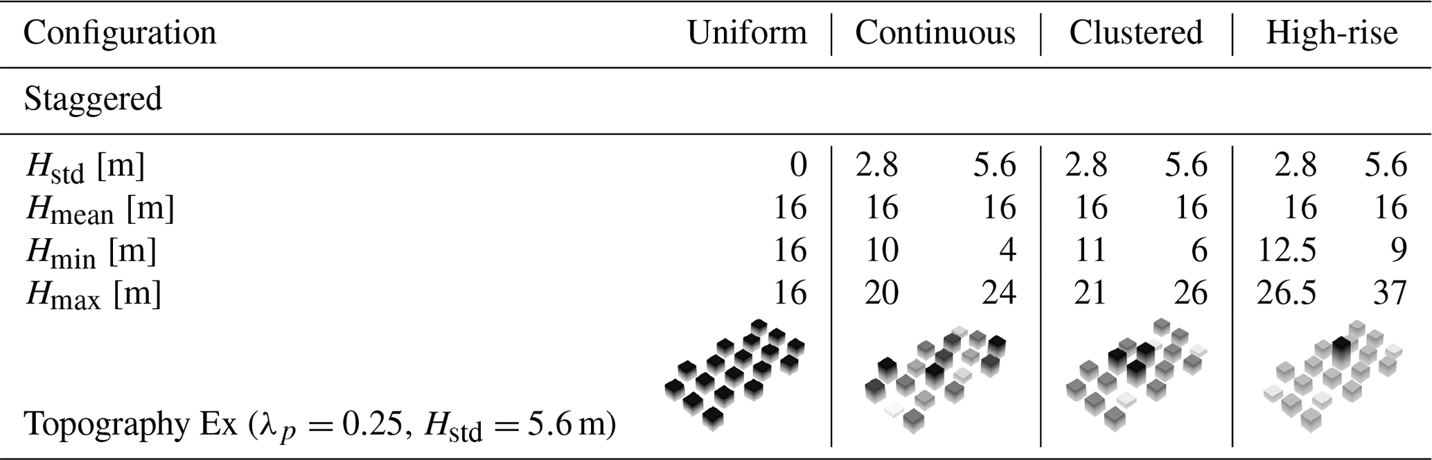
The detailed design of building arrays can be found in Lu et al. (2023a) and is briefly explained here: while maintaining the same volume of roughness elements (i.e., same mean building height, H_mean=16 m), we consider three height distributions, i.e., $H_{\mathrm{std}}\in [\mathrm{0}\mathrm{m},\mathrm{2.8}\mathrm{m},\mathrm{5.6}\mathrm{m}]$, which result in different maximum building height H_max. Additionally, we consider three types of urban arrays: (a) continuous distribution of building height with a relatively low H_max; (b) clustered configuration with two clusters (three buildings) of low and tall building blocks; and (c) high-rise configuration, featuring one tall and a cluster (three) of low building blocks. Each configuration is then run with seven urban packing densities, i.e., ${\mathit{\lambda }}_p\in [\mathrm{0.0625},\mathrm{0.1111},\mathrm{0.16},\mathrm{0.25},\mathrm{0.35},\mathrm{0.4444},\mathrm{0.64}]$, which yields a total of 49 simulation cases. Details of the configurations considered are shown in Table 1.

Table 1 Dataset details for 49 urban arrays discussed in this study. Four building height arrangements (uniform, continuous, clustered, and high-rise) with two standard deviations of height configurations are considered. The maximum H_max and minimum H_min building heights and a three-dimensional view of an example (λ_p=0.25) are shown below each category.

3 Assessment of the multi-layer urban canopy model (MLUCM)

In mesoscale climate models, flow through canopies is often simulated at scales much larger than the typical surface processes, such as turbulent eddies and obstacle wakes. A common approach to derive parameterizations is to apply a time averaging over an interval longer than the scale of the slowest eddies and a spatial averaging over a length larger than the typical spatial deviations in the flow (Raupach and Shaw, 1982; Finnigan, 1985). For momentum, the Reynolds decomposition is first applied to the three-dimensional instantaneous equations that decompose mean flow quantities ($\stackrel{\mathrm{‾}}{\mathit{\varphi }}$) from their fluctuating components (ϕ^′, time or ensemble averaging, $\mathit{\varphi }=\stackrel{\mathrm{‾}}{\mathit{\varphi }}+{\mathit{\varphi }}^{\prime }$). Then, flow properties are spatially averaged to match a grid cell of a mesoscale model (horizontal averaging, $\stackrel{\mathrm{‾}}{\mathit{\varphi }}=\langle \stackrel{\mathrm{‾}}{\mathit{\varphi }}\rangle +\stackrel{\mathrm{̃}}{\mathit{\varphi }}$, where $\stackrel{\mathrm{̃}}{\mathit{\varphi }}$ is termed a dispersive component).

In urban canopies where the volume fraction occupied by obstacles is not negligible, the intrinsic average (Schmid et al., 2019) that excludes the roughness fraction in the spatial averaging is more favorable given that additional terms compensating for the volume fraction occupied by roughness elements in the canopy are included Blunn et al. (2022). The friction Reynolds number ($Re=u_{\mathit{\tau }}{H}_T/\mathit{\nu }$, where u_τ∼0.21 m s⁻¹ is the friction velocity, H_T is the domain height, and ν is the kinematic viscosity) of the flow dataset is large enough (10⁶) to neglect viscous stress on momentum and molecular flux on scalars. The resulting one-dimensional representation of the momentum and passive scalar equation assuming horizontal homogeneity, negligible Coriolis effect, and buoyancy force reads

$$\begin{array}{}\text{(1)}& {\displaystyle }\begin{array}{rl}{\displaystyle \frac{\partial \langle \overline{u}\rangle }{\partial t}}& =-{\displaystyle \frac{\partial \left(〈\stackrel{\mathrm{‾}}{u^{\prime }{w}^{\prime }}〉+〈\stackrel{\mathrm{̃}}{u}\stackrel{\mathrm{̃}}{w}〉\right)}{\partial z}}-{\displaystyle \frac{\langle \stackrel{\mathrm{‾}}{u^{\prime }{w}^{\prime }}\rangle +\langle \stackrel{\mathrm{̃}}{u}\stackrel{\mathrm{̃}}{w}\rangle }{\mathit{\gamma }}}{\displaystyle \frac{\partial \mathit{\gamma }}{\partial z}}\\ & +f_i-{\displaystyle \frac{\mathrm{1}}{\mathit{\rho }}}〈{\displaystyle \frac{\partial \stackrel{\mathrm{‾}}{P}}{\partial x_i}}〉\end{array}\text{(2)}& {\displaystyle \frac{\partial \langle \overline{c}\rangle }{\partial t}}=-{\displaystyle \frac{\partial \left(〈\stackrel{\mathrm{‾}}{c^{\prime }{w}^{\prime }}〉+〈\stackrel{\mathrm{̃}}{c}\stackrel{\mathrm{̃}}{w}〉\right)}{\partial z}}-{\displaystyle \frac{\langle \stackrel{\mathrm{‾}}{c^{\prime }{w}^{\prime }}\rangle +\langle \stackrel{\mathrm{̃}}{c}\stackrel{\mathrm{̃}}{w}\rangle }{\mathit{\gamma }}}{\displaystyle \frac{\partial \mathit{\gamma }}{\partial z}}+c_i,\end{array}$$

where ρ is the air density, u and w are the streamwise and vertical velocity so that $\langle \stackrel{\mathrm{‾}}{u^{\prime }{w}^{\prime }}\rangle$ and $\langle \stackrel{\mathrm{̃}}{u}\stackrel{\mathrm{̃}}{w}\rangle$ form the spatially averaged turbulent and dispersive Reynolds stress, respectively. The first term on the RHS of both equations represents vertical transport events, while the second term is a term that compensates for volume change in the intrinsic averaging, where $\mathit{\gamma }\left(z\right)=\mathrm{1}-{\mathit{\lambda }}_p\left(z\right)$ is the fluid fraction at the vertical index z. The third term, f_i and c_i, accounts for external sources or sinks, such as pressure gradient driving the flow and surface emission of pollutants. The fourth term of Eq. (1) represents the pressure drop between windward and leeward building facets (Santiago and Martilli, 2010b), which accounts for momentum sink due to building-induced drag rising from spatial averaging over the momentum equation. The multi-layer model is designed to relate terms in Eq. (1) to the variation of urban surface, where the vertical diffusion of momentum (Sects. 3.1 and 3.2) and drag (Sect. 3.3) are parameterized.

3.1 Characterization of the eddy diffusivity for different flow statistics

The Reynolds averaging over the momentum equation yields nonlinear terms that must be parameterized to close the equation. The most common approach in parameterizing the Reynolds stress in UCMs is based on K theory (as also seen in models compared in Best and Grimmond, 2015, Lipson et al., 2023) to represent the efficiency of turbulent transports by employing the eddy-diffusivity coefficient together with the vertical gradient of the flow properties (for momentum, $\langle K_{\mathrm{m}}\rangle =-〈\stackrel{\mathrm{‾}}{u^{\prime }{w}^{\prime }}〉/〈\frac{\partial \stackrel{\mathrm{‾}}{u}}{\partial z}〉$). In a variety of ways specifying the eddy diffusivity, the 1.5-order closure (Martilli et al., 2002) assuming the transport strength related to the turbulence intensity is commonly employed for urban canopy flow as follows:

$$\begin{array}{}\text{(3)}& K_{\mathrm{m}}=C_k{l}_k\langle k{\rangle }^{\mathrm{1}/\mathrm{2}},\end{array}$$

where C_k is a model constant, l_k is a turbulent length scale, and k is TKE that has to be prognostically obtained during the simulation following Eq. (4).

$$\begin{array}{}\text{(4)}& \begin{array}{rl}{\displaystyle \frac{\partial \langle \overline{k}\rangle }{\partial t}}& =-{\displaystyle \frac{\partial \left(〈\stackrel{\mathrm{‾}}{k^{\prime }{w}^{\prime }}〉+〈\stackrel{\mathrm{̃}}{k}\stackrel{\mathrm{̃}}{w}〉\right)}{\partial z}}-{\displaystyle \frac{\langle \stackrel{\mathrm{‾}}{k^{\prime }{w}^{\prime }}\rangle +\langle \stackrel{\mathrm{̃}}{k}\stackrel{\mathrm{̃}}{w}\rangle }{\mathit{\gamma }}}{\displaystyle \frac{\partial \mathit{\gamma }}{\partial z}}\\ & -〈\stackrel{\mathrm{‾}}{u_i^{\prime }{u}_j^{\prime }}〉{\displaystyle \frac{\partial 〈\stackrel{\mathrm{‾}}{u_i}〉}{\partial x_j}}-〈\stackrel{\mathrm{̃}}{u_i^{\prime }{u}_j^{\prime }}{\displaystyle \frac{\partial \stackrel{\mathrm{̃}}{u_i}}{\partial x_j}}〉-D_k-\langle \overline{\mathit{\epsilon }}\rangle \end{array}\end{array}$$

Similar to the momentum equation (Eq. (1)), the first two terms on the RHS represent the transport of TKE, followed by two terms for shear and dispersive TKE production, respectively. D_k represents the source of TKE generated through the interaction with the buildings and the airflow, while the last term $\langle \overline{\mathit{\epsilon }}\rangle$ is the viscous dissipation of TKE that can be parameterized as

$$\begin{array}{}\text{(5)}& \langle \overline{\mathit{\epsilon }}\rangle =C_{\mathit{\epsilon }}{\displaystyle \frac{\langle \overline{k}{\rangle }^{\mathrm{3}/\mathrm{2}}}{l_{\mathit{\epsilon }}}},\end{array}$$

where C_ε and l_ε are the model constant and the dissipation length scale, respectively, and have a relationship with turbulent length scale based on the turbulent viscosity C_μ (Santiago and Martilli, 2010b) that measures the relative strength of viscous dissipation over turbulent transport:

$$\begin{array}{}\text{(6)}& C_k{l}_k=C_{\mathit{\mu }}{\displaystyle \frac{l_{\mathit{\epsilon }}}{C_{\mathit{\epsilon }}}}.\end{array}$$

To date, most models assume the same value for the diffusion coefficient in the momentum, TKE, and scalar equations, possibly due to the lack of data on TKE and scalar budget terms (note that the explicit evaluation of TKE transport and diffusivity, in particular, is only possible from numerical simulations that resolve third-order moments, e.g., LES and direct numerical simulations (DNS)). However, previous LES analyses of urban flow indicated a different transport efficiency of varying flow properties (Nazarian et al., 2020). Accordingly, we distinguish between three diffusion coefficients as

$$\begin{array}{}\text{(7a)}& {\displaystyle }& {\displaystyle }\langle K_{\mathrm{m}}\rangle =-〈\stackrel{\mathrm{‾}}{u^{\prime }{w}^{\prime }}〉/〈{\displaystyle \frac{\partial \stackrel{\mathrm{‾}}{u}}{\partial z}}〉=-〈\stackrel{\mathrm{‾}}{u^{\prime }{w}^{\prime }}〉/\left({\displaystyle \frac{\partial \langle \stackrel{\mathrm{‾}}{u}\rangle }{\partial z}}+{\displaystyle \frac{\langle \stackrel{\mathrm{‾}}{u}\rangle }{\mathit{\gamma }}}{\displaystyle \frac{\partial \mathit{\gamma }}{\partial z}}\right)\text{(7b)}& {\displaystyle }& {\displaystyle }\langle K_c\rangle =-〈\stackrel{\mathrm{‾}}{c^{\prime }{w}^{\prime }}〉/〈{\displaystyle \frac{\partial \stackrel{\mathrm{‾}}{c}}{\partial z}}〉=-〈\stackrel{\mathrm{‾}}{c^{\prime }{w}^{\prime }}〉/\left({\displaystyle \frac{\partial \langle \stackrel{\mathrm{‾}}{c}\rangle }{\partial z}}+{\displaystyle \frac{\langle \stackrel{\mathrm{‾}}{c}\rangle }{\mathit{\gamma }}}{\displaystyle \frac{\partial \mathit{\gamma }}{\partial z}}\right)\text{(7c)}& {\displaystyle }& {\displaystyle }\langle K_k\rangle =-〈\stackrel{\mathrm{‾}}{k^{\prime }{w}^{\prime }}〉/〈{\displaystyle \frac{\partial \stackrel{\mathrm{‾}}{k}}{\partial z}}〉=-〈\stackrel{\mathrm{‾}}{k^{\prime }{w}^{\prime }}〉/\left({\displaystyle \frac{\partial \langle \stackrel{\mathrm{‾}}{k}\rangle }{\partial z}}+{\displaystyle \frac{\langle \stackrel{\mathrm{‾}}{k}\rangle }{\mathit{\gamma }}}{\displaystyle \frac{\partial \mathit{\gamma }}{\partial z}}\right).\end{array}$$

The turbulent fluxes, vertical gradient, and eddy diffusivity of momentum, TKE, and scalars are shown in Fig. 1 for staggered-uniform configurations for cubic buildings. The roughness flow over other building shapes such as cuboids (Blunn et al., 2022; Li and Bou-Zeid, 2019), cylinders (Agbaglah and Mavriplis, 2019), and spheres (Ye et al., 2016) exhibits different transport behavior. However, most buildings are a combination of cuboids (Oke et al., 2017), and non-urban roughness flow is not suitable to inform urban parameterization. Therefore, the transport behavior over non-cuboid roughness is outside of the current scope. Note that the profiles over other designs with building height variability (not shown here) share similar characteristics. Therefore, we chose the uniform-height layout to better reveal the difference among flow properties. Within the canopy, the turbulent fluxes of momentum and TKE are predominantly negative, reflecting downgradient transports driven by their differing production and destruction mechanisms. The turbulent fluxes of passive scalars are positive due to the surface emission being the only source and exhibiting a minor variation across different densities. The eddy diffusivity of scalars (K_c) and momentum (K_m) maintains a similar shape as a result of the relatively simpler mechanism in their production, destruction, and transport, which justifies the simplification (K_c∼K_m) that is consistent with Li and Bou-Zeid (2019). However, the eddy diffusivity of TKE (K_k) demonstrates a greater complexity with some negative values at the ground and canopy interface that marks the counter-gradient transport of TKE indicating two vital local shear production regions: (a) the canopy-top shear zone is relatively well-studied and is induced by clearings of roughness elements (Giometto et al., 2016) and the (b) near-ground shear zone that is unique in medium-dense layouts (λ_p≤0.25) where flow reversal appears and counteracts with the pressure gradient, inducing a significant shear source of TKE (Lu et al., 2023a). This lack of consideration of the near-ground flow features partially explains the underestimation of local TKE seen in Nazarian et al. (2020) and can be mitigated by imposing a height-dependent model constant (e.g., Glazunov et al., 2021), but is beyond the scope of this study that aims to refine the turbulent transport characterization within the whole canopy. Apart from the near-ground and canopy-top inversion, K_k shares a similar shape with K_m but presents a significantly larger magnitude, which indicates that models using unified K underestimate the transport of TKE and require closer characterization. The distinct behavior of K_m in the densest case (purple lines in Fig. 1c) comes from the positive gradient of streamwise velocity in the middle of the canopy and positive Reynolds stress in the lower canopy that is hard to characterize. Such a high density is not rare, especially in some European and South American cities. However, realistic neighborhoods with extremely high density typically exhibit varied horizontal arrangements, leading to different flow characteristics from idealized building blocks (Lu et al., 2023b).

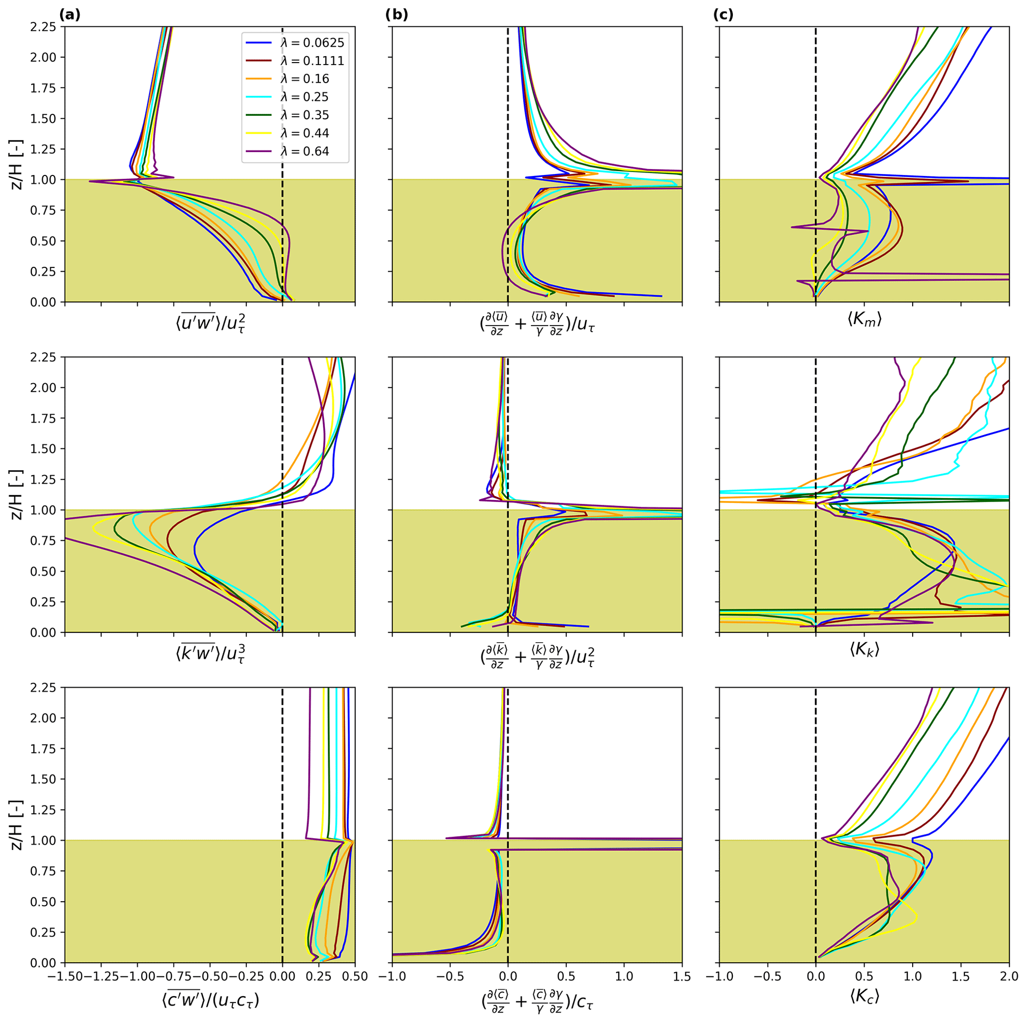
Figure 1 Vertical profiles of turbulent flux (first column), vertical gradient (second column), and eddy diffusivity (third column) of momentum, TKE, and scalar flux from Eq. (7) evaluated over uniform-staggered configurations. The yellow-shaded range indicates the mean building height. The x axis is limited to show most profiles for better presentability. Values are off the axis limit at the canopy top due to the strong shear zone.

Following the parameterization of length scales in Nazarian et al. (2020), we average the profile of eddy diffusivities shown in Fig. 1 up to H_mean to reveal the integral behavior of transport behaviors across configurations. Figure 2 presents the scatter of the vertically averaged eddy diffusivity for momentum K_m,T and TKE K_k,T without considering dispersive flux, and these include the dispersive contribution ($K_{\mathrm{m},T+D}$ and $K_{k,T+D}$). Characterization of dispersive fluxes within the K-theory framework enhances the exchange rate of flow properties, which agrees with previous studies such as Akinlabi et al. (2022) where the dispersive flux is mostly downward.

The magnitude of eddy diffusivity for TKE is ∼3.5 times higher than that for momentum (note the different vertical ranges for momentum and TKE in Fig. 2). This considerable difference demonstrates a significant contrast to the parameterization strategy in Nazarian et al. (2020) that assumed $K_{\mathrm{m},T+D}=K_{k,T+D}$, which results in underestimations of TKE within the canopy. In addition, unlike $K_{\mathrm{m},T+D}$, which generally decreases with urban density before the layout becomes very dense, $K_{k,T+D}$ exhibits a less decisive trend to density. The magnitude difference and variations over densities between $K_{\mathrm{m},T+D}$, and $K_{k,T+D}$ urge for a distinction in their parameterizations.

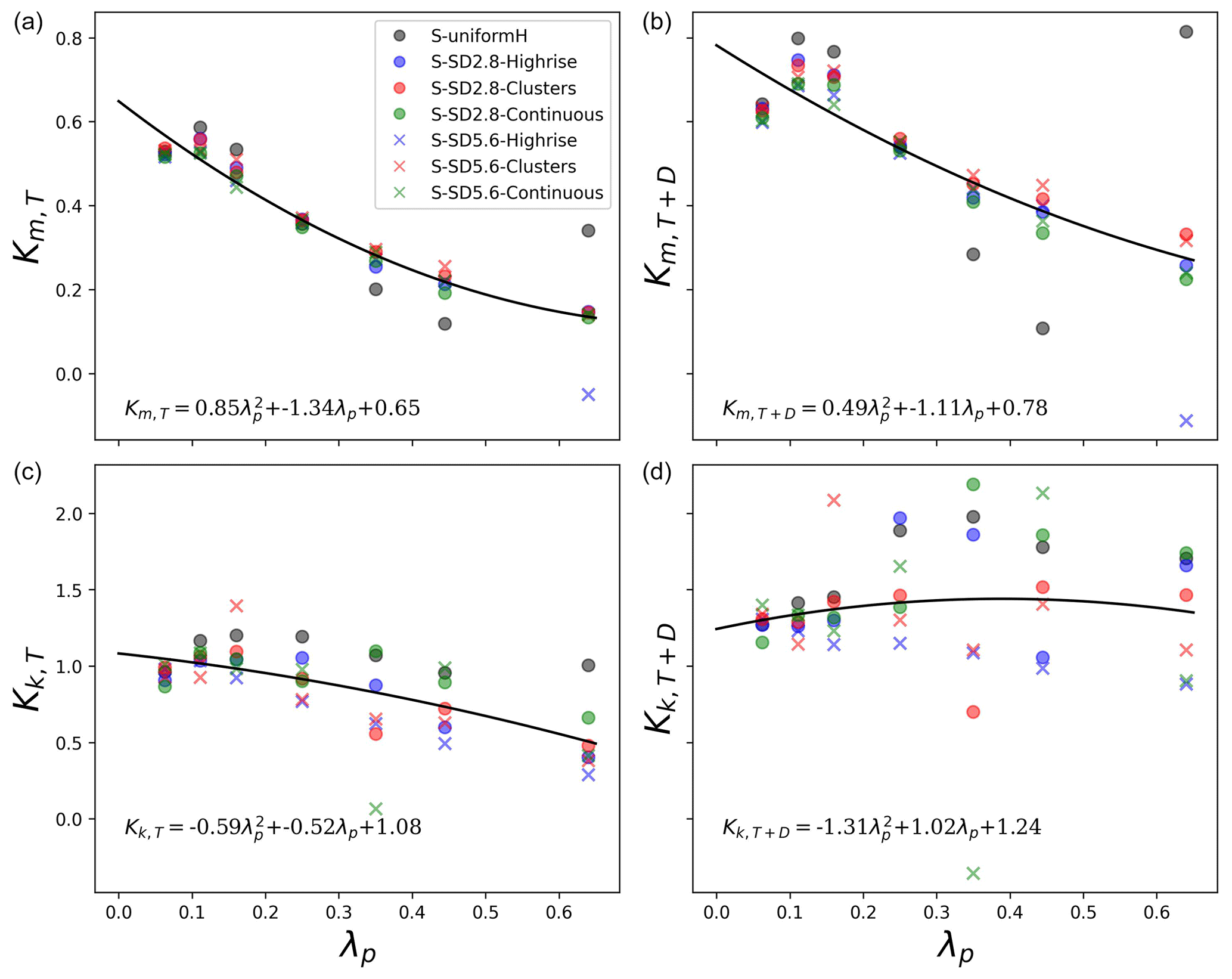
Figure 2 Canopy-averaged eddy diffusivity for momentum and TKE with ($K_{\mathrm{m},T+D}$ and $K_{k,T+D}$) and without (K_m,T and K_k,T) additional consideration of the dispersive component. Black lines indicate second-order polynomial regressions over the means of seven configurations under the same densities where the regression equation is shown at the bottom of each subplot.

The eddy diffusivity was not directly parameterized under the 1.5-order closure framework developed in Martilli et al. (2002) but as a turbulent length scale correlated with the dissipation length scale in Eq. (6) (i.e., $C_k{l}_k=C_{\mathit{\mu }}\frac{l_{\mathit{\epsilon }}}{C_{\mathit{\epsilon }}}$). Here we follow the same approach as in Nazarian et al. (2020) to parameterize the turbulent viscosity (C_μ) and dissipation length scale ($\frac{l_{\mathit{\epsilon }}}{C_{\mathit{\epsilon }}}$) to obtain the turbulent length scale (C_kl_k). Considering that the parameterization for dissipation length scale is the same across the scenarios considered in Table 2, the difference in the transport efficiency demonstrated in Sects. 3.1 and 3.2 can be expressed as the difference in the turbulent viscosity (C_μ), as shown in Fig. 3.

Figure 3 shows the turbulent viscosity calculated in 49 idealized urban arrays binned over densities for better presentation, where the original parameterization with seven uniform-height cases (Nazarian et al., 2020) is shown in green lines. Generally, C_μ increases with density over sparse and medium layouts, which indicates the overweighting trend of viscous dissipation of TKE over the turbulent transport that is consistent with the transition of the flow regime (Oke et al., 2017). Meanwhile, denser layouts amplify the impact of building height variability, leading to a higher standard deviation among binned scenarios, which is consistent with Lu et al. (2023a). Turbulent viscosity for momentum lumping the dispersive flux $C_{\mathit{\mu },K_{\mathrm{m},T+D}}$ shows a good agreement with that from Nazarian et al. (2020) except for the peaking at higher density. Due to the separate explicit characterization of the building-induced dispersive momentum transport, $C_{\mathit{\mu },K_{\mathrm{m},T+S}}$ is slightly lower than $C_{\mathit{\mu },K_{\mathrm{m},T+D}}$ but shows a similar shape. The turbulent viscosity of TKE ($C_{\mathit{\mu },K_{k,T+D}}$) is about 3.5 times higher than that of momentum (note the difference on the y-axis limit) and shows exponential growth over density.

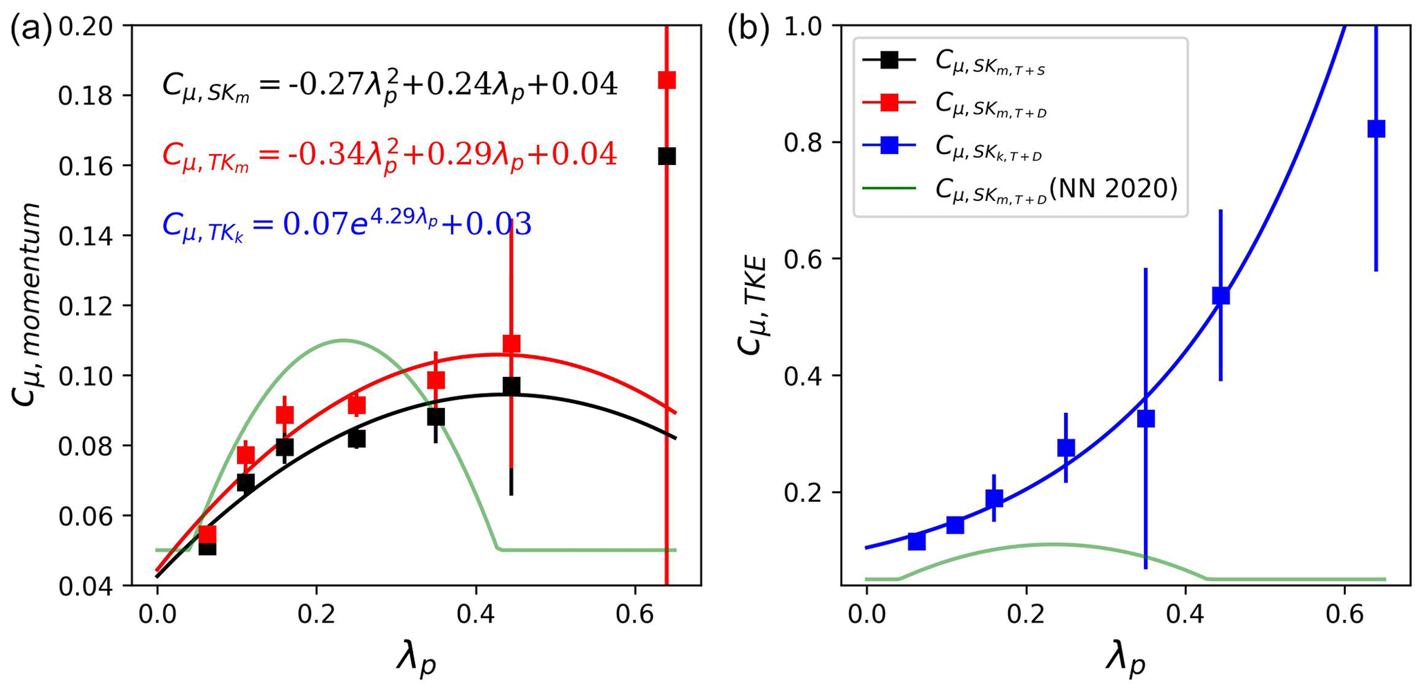
Figure 3 Canopy-averaged turbulent viscosity for momentum and TKE. Panel (a) shows the turbulent viscosity of momentum where the red and black dots indicate evaluations adding the dispersive and turbulent fluxes ($C_{\mathit{\mu },T{K}_{\mathrm{m}}}$) and sampling out the fraction of building-induced dispersive flux ($C_{\mathit{\mu },S{K}_{\mathrm{m}}}$) and lumping the residue, respectively. Panel (b) shows the turbulent viscosity of TKE, lumping the dispersive component. Data points are binned by their ground density λ_p(z=0), where the vertical line attached to each square indicates the standard deviation among the data points binned. Green lines indicate the parameterization from Nazarian et al. (2020).

3.2 Characterization of the dispersive momentum transport

The momentum transport in urban canopy flow is also modulated by its spatial variability (Eq. 1) induced by the rigid volume of roughness elements that is hard to characterize due to its extreme heterogeneity (Poggi and Katul, 2008b). Nevertheless, flow heterogeneity is not unique to the urban boundary layer but is prevalent in the real-world atmosphere layer due to the surface heating and has been well characterized in PBL parameterizations (e.g., Han and Bretherton, 2019). In the context of convective boundary layer parameterization, the eddy diffusivity (ED) approach based on K theory (as discussed in Sect. 3.1) has been successful in representing neutral and surface boundary layers that promote more homogeneous and isotropic turbulence (Fig. 4a). On the other hand, the flow heterogeneity induced by convection from thermal forcing and moisture phase change has been successfully captured by the mass-flux (MF) approach (Siebesma et al., 2007). In the effort to model both atmospheric conditions coexisting in PBL, an eddy-diffusivity mass-flux (EDMF) scheme has been developed by partitioning flow fluctuations into contributions from local turbulent mixing (ED) and non-local coherent rising and descending air parcels (MF, Lopez‐Gomez et al., 2020; Lu, 2019).

This section explores this alternative approach to characterize the dispersive momentum flux, other than the pragmatic approach developed in Nazarian et al. (2020); Simón-moral et al. (2016), by considering dispersive transports as mass-flux components under the framework of the EDMF scheme. The dispersive transports of momentum (Fig. 4b) in the urban boundary layer are induced by coherent motions near the building facets and present a strong local distribution that resembles the patchy coherent structures induced by thermal forcing in PBL. Therefore, the similarity in flow heterogeneity between UCL and PBL implies a phenomenological analogy, which favors the introduction of the EDMF approach to multi-layer UCMs. Following the formulation in Siebesma et al. (2007), the dispersive flux of momentum is firstly decomposed into individual plumes (a_i) enclosing coherent motions with strength $\left(\stackrel{\mathrm{‾}}{u_i}-\langle \stackrel{\mathrm{‾}}{u}\rangle \right)\left(\stackrel{\mathrm{‾}}{w_i}-\langle \stackrel{\mathrm{‾}}{w}\rangle \right)$ and then sorted into upward (positive, with a fraction of a_u) and downward (negative, with a fraction of a_d) contributions. The dispersive flux of momentum then reads

$$\begin{array}{}\text{(8)}& \begin{array}{rl}\langle \stackrel{\mathrm{̃}}{u}\stackrel{\mathrm{̃}}{w}\rangle & =\sum _i{a}_{\mathrm{i}}\left(\stackrel{\mathrm{‾}}{u_i}-\langle \stackrel{\mathrm{‾}}{u}\rangle \right)\left(\stackrel{\mathrm{‾}}{w_i}-\langle \stackrel{\mathrm{‾}}{w}\rangle \right)\\ & =a_{\mathrm{u}}\langle \stackrel{\mathrm{̃}}{u}\stackrel{\mathrm{̃}}{w}{\rangle }_{\mathrm{u}}+a_{\mathrm{d}}\langle \stackrel{\mathrm{̃}}{u}\stackrel{\mathrm{̃}}{w}{\rangle }_{\mathrm{d}}{a}_{\mathrm{u}}+a_{\mathrm{d}}=\mathrm{1}\end{array}.\end{array}$$

Note that, for simplicity, the entrainment process (Abdella and Petersen, 2000) that represents scalar transport between subdomains (between dispersive structures and the turbulent environment) is not considered here. Using the mass-flux approach to characterize dispersive momentum flux requires the fraction ($a_{\mathrm{u}}+a_{\mathrm{d}}=\mathrm{1}$) and strength ($\langle \stackrel{\mathrm{̃}}{u}\stackrel{\mathrm{̃}}{w}{\rangle }_{\mathrm{u}}$, $\langle \stackrel{\mathrm{̃}}{u}\stackrel{\mathrm{̃}}{w}{\rangle }_{\mathrm{d}}$) of those coherent flow motions to be parameterized based on the variation of the urban arrangement. An example of the spatial distribution of turbulent and dispersive momentum flux is shown in Fig. 4 for the S-highrise-SD56 configuration of density λ_p=0.25 sampled at z=15 m.

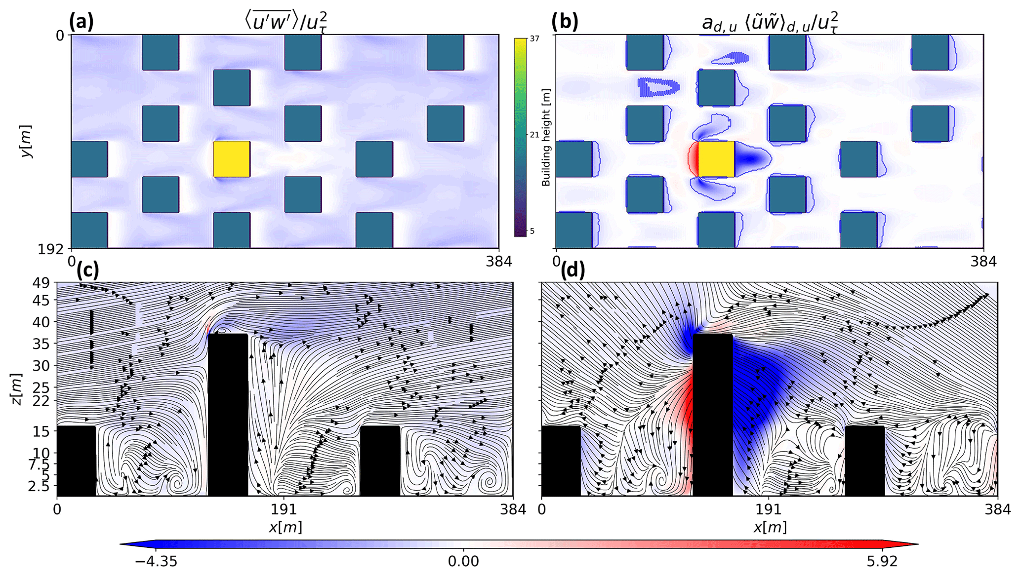
Figure 4 An example of horizontal and vertical field sampled at 93.8 % of the mean building height (z=15 m and y=110 m, respectively), for the S-highrise-SD56 configuration of density λ_p=0.25. The left panels (a, c) show the turbulent flux of momentum ((a) $〈\stackrel{\mathrm{‾}}{u^{\prime }{w}^{\prime }}〉/u_{\mathit{\tau }}^{\mathrm{2}}$=-0.6052) that forms the “background” transport events, with the title showing the spatial average. The right panels (b, d) show the dispersive flux that forms “hot spot” transport events ((b) $a_{\mathrm{d}}\langle \stackrel{\mathrm{̃}}{u}\stackrel{\mathrm{̃}}{w}{\rangle }_{\mathrm{d}}/u_{\mathit{\tau }}^{\mathrm{2}}$=-0.2122, $a_{\mathrm{u}}\langle \stackrel{\mathrm{̃}}{u}\stackrel{\mathrm{̃}}{w}{\rangle }_{\mathrm{u}}/u_{\mathit{\tau }}^{\mathrm{2}}=\mathrm{0.0253}$), with the contribution from upward and downward transport indicated in the title. Regions enclosed by red and blue lines indicate values sampled with a 50 % CDF. Vectors in the bottom left (c) panel show the mean velocity direction, whereas those in the bottom right show the direction of the dispersive velocity ($\stackrel{\mathrm{̃}}{u}=\stackrel{\mathrm{‾}}{u}-\langle \stackrel{\mathrm{‾}}{u}\rangle$).

Unlike the turbulent momentum flux, which shows a uniform downward transport with an indecisive correlation with the local roughness elements, a portion of the dispersive counterpart is directly connected to the local roughness, whereas the rest remains relatively homogeneous. Therefore, a proper sampling filter should be applied to enclose these regions before gathering flow properties for parameterization. Again, we adopt a common sampling approach in the development of the EDMF (Couvreux et al., 2010; Sušelj et al., 2012) based on the joint cumulative probability density function (CDF) of the dispersive velocities ($\stackrel{\mathrm{̃}}{u},\stackrel{\mathrm{̃}}{w}$).

$$\begin{array}{}\text{(9)}& \mathrm{CDF}\left(\right(\stackrel{\mathrm{̃}}{u},\stackrel{\mathrm{̃}}{w}\left)\right)=\underset{{\stackrel{\mathrm{̃}}{u}}_{\min }}{\overset{{\stackrel{\mathrm{̃}}{u}}_{\max }}{\int }}\underset{{\stackrel{\mathrm{̃}}{w}}_{\min }}{\overset{{\stackrel{\mathrm{̃}}{w}}_{\max }}{\int }}\mathrm{PDF}(\stackrel{\mathrm{̃}}{u},\stackrel{\mathrm{̃}}{w})\mathrm{d}\stackrel{\mathrm{̃}}{u}\mathrm{d}\stackrel{\mathrm{̃}}{w}=\mathrm{1}\end{array}$$

The CDF can be adjusted from [0,1] that corresponds to different integration ranges of dispersive streamwise and vertical velocity (Eq. 9). By lowering the CDF, the sampled regions are adjusted smaller only to enclose regions with outstanding strength. We tested a range of cut-off values of $\mathrm{CDF}\in [\mathrm{0.3},\mathrm{0.4},\mathrm{0.5},\mathrm{0.6},\mathrm{0.7}]$ (test results are shown in the Appendix and in the Supplement), and a cut-off value here is determined as 0.5 for all cases considered. Figure 4b shows the sampled upward and downward transports enclosed by red and blue lines, respectively.

The sampling filter aims to capture the building-induced component of the dispersive momentum flux that K theory cannot characterize. Here, we test the correlation between dispersive streamwise velocity ($\stackrel{\mathrm{̃}}{u}$) and vertical velocity ($\stackrel{\mathrm{̃}}{w}$) to show how the urban structures modify the statistical distribution of dispersive fluxes and the corresponding characterization fulfilled by the sampling. Figure 5 shows the 2D CDF distribution for S-highrise-SD56 configuration of density λ_p=0.25. The distribution exhibits a more eccentric behavior along the vertical range, with

1. One tail growing stronger and thinner at the third quadrant ($\stackrel{\mathrm{̃}}{u}<\mathrm{0},\stackrel{\mathrm{̃}}{w}<\mathrm{0}$) representing the blockage effects of the frontal area of the roughness (Fig. 4d), which is well-captured by the sampling strategy (red squares in Fig. 5). The height distribution of building blocks can explain the thinner trend and reflect how the dispersive flux responds to the urban vertical structure.

2. A relatively symmetric elongated region at the second ($\stackrel{\mathrm{̃}}{u}<\mathrm{0},\stackrel{\mathrm{̃}}{w}>\mathrm{0}$) and fourth quadrant ($\stackrel{\mathrm{̃}}{u}>\mathrm{0},\stackrel{\mathrm{̃}}{w}<\mathrm{0}$) representing the leeward flow cavity (Fig. 4b, characterized by the sampled flux at most heights) and flow divergence at the lateral facets (represented by the sampled flux at 2.5 m), respectively. The elongation of both sides reflects a more irregular distribution of downward dispersive flux with heights, which is consistent with the analysis in Lu et al. (2023a).

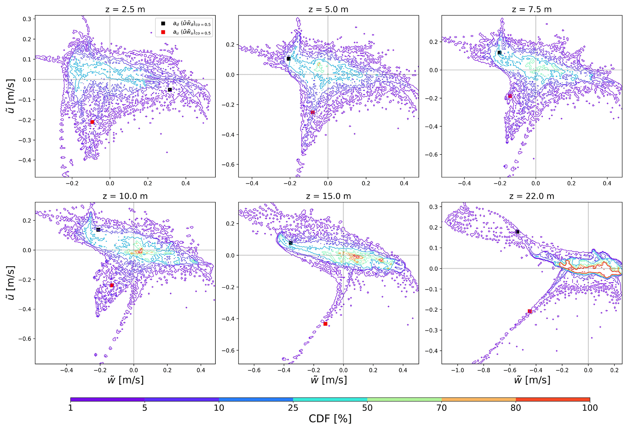
Figure 5 Contour plot showing the two-dimensional histograms of the CDF of the dispersive velocities at 2.5, 5, 7.5, 10, 15, and 22 m. The integral of the PDF (from outside to the mean value) within the area is delineated by isolines on the logarithmic scale. The black/red squares depict the averaged dispersive flux over the sampled regions to represent the strength of the gradient and counter-gradient transport parameterized in MLUCM v3.0.

After subtracting dispersive structures from the sampled regions, the rest of the relatively homogeneous regions may safely resort back to the lumping approach and update Eq. (8) with Eq. (10):

$$\begin{array}{}\text{(10)}& \begin{array}{rl}\langle \stackrel{\mathrm{̃}}{u}\stackrel{\mathrm{̃}}{w}\rangle & ={\left(a_{\mathrm{u}}\langle \stackrel{\mathrm{̃}}{u}\stackrel{\mathrm{̃}}{w}{\rangle }_{\mathrm{u}}\right)}_{\mathrm{co}=\mathrm{0.5}}+{\left(a_{\mathrm{d}}\langle \stackrel{\mathrm{̃}}{u}\stackrel{\mathrm{̃}}{w}{\rangle }_{\mathrm{d}}\right)}_{\mathrm{co}=\mathrm{0.5}}\\ & +{\left(\langle \stackrel{\mathrm{̃}}{u}\stackrel{\mathrm{̃}}{w}\rangle \right)}_{\mathrm{residue}}.\end{array}\end{array}$$

We speculate the reason that dispersive flux has long been ill represented in UCMs is attributed to the inappropriate scaling with the turbulent flux (e.g., Poggi and Katul, 2008b), which usually yields a small fraction without recognizing these two processes are controlled by very different physical processes. Alternatively, the dispersive perturbations are caused by the pressure fields associated with the topography or the changed resistance to flow through the canopy (Finnigan et al., 2015; Finnigan and Shaw, 2008), which implies a possibility of scaling its strength to the external pressure gradient. This was only made possible recently due to the increased computational power and awareness of intrinsic urban heterogeneity (Boeing, 2019; Lu et al., 2023b). Therefore, we hypothesize the strength of sampled flow motions can be parameterized by pressure gradient and urban morphological parameters as Eq. (11):

$$\begin{array}{}\text{(11)}& a_{\mathrm{u},\mathrm{d}}\langle \stackrel{\mathrm{̃}}{u}\stackrel{\mathrm{̃}}{w}{\rangle }_{\mathrm{u},\mathrm{d}}=f\left(z,{\displaystyle \frac{\partial \stackrel{\mathrm{‾}}{p}}{\partial x}},{\mathit{\lambda }}_p,H_{\max ,\mathrm{mean},\mathrm{std}}\right).\end{array}$$

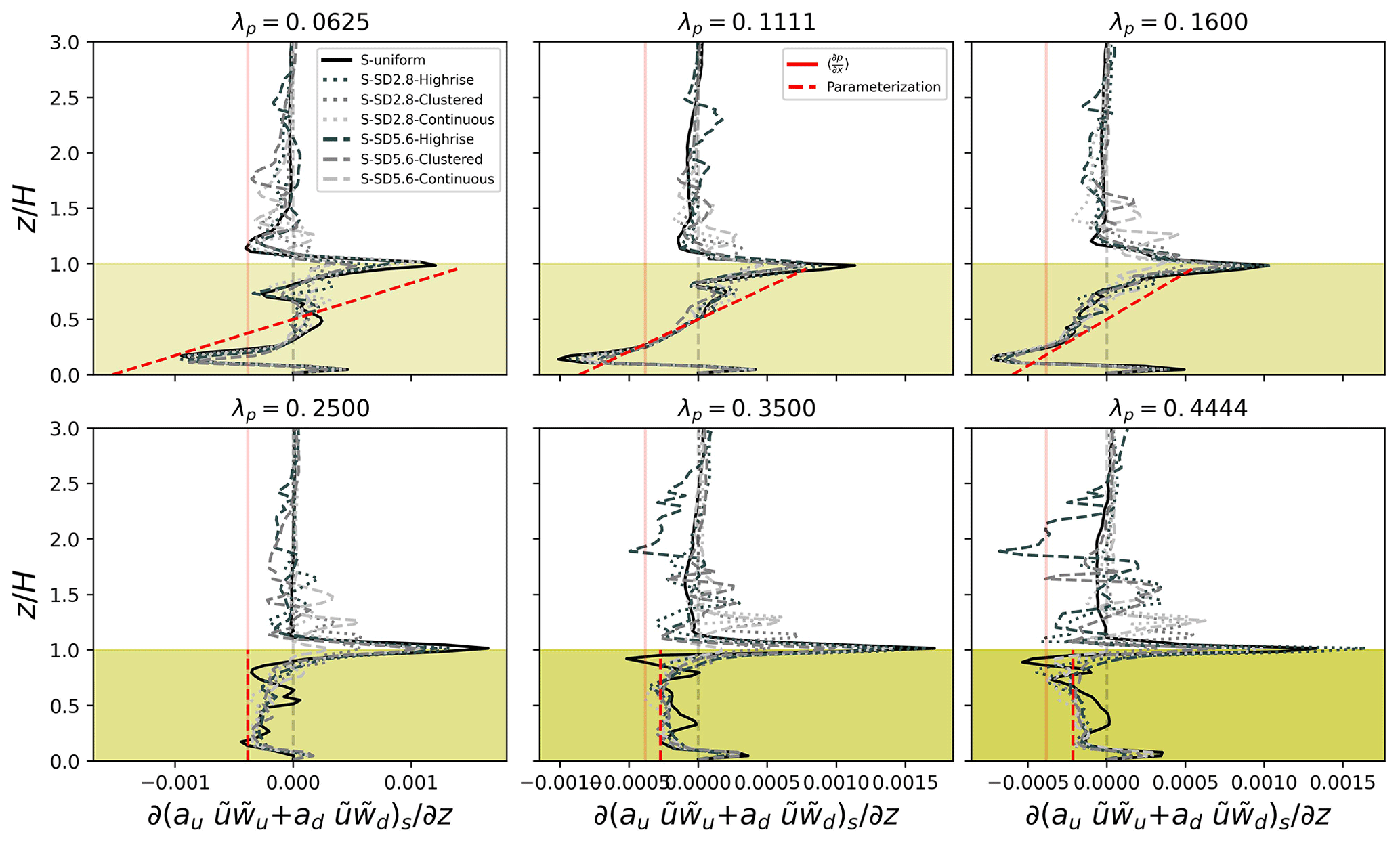
Figure 6 Vertical profiles of sampled downward and upward dispersive momentum flux (gray-scale lines) for seven building height configurations covering ${\mathit{\lambda }}_p\in [\mathrm{0.0625},\mathrm{0.4444}]$. The range of mean building height is marked in yellow shades with the transparency following the λ_p. Diminished red lines indicate the strength of the external pressure gradient constant with height. Dashed red lines show the parameterization from Eq. (12).

To gain a direct impression of how the sampled dispersive motions scale with the pressure gradient, we present the profile of the vertical gradient of the sum of two sampled terms from Eq. (10) in Fig. 6. The variation of the dispersive momentum transport exhibits a strong dependence on the flow regime but decouples with the turbulence level (not shown here; see Figs. 9–11 from Lu et al. (2023b) for spatial pattern of TKE as well as turbulent and dispersive momentum flux). The sampled dispersive motion is of a similar magnitude to the only driver in our experiments – pressure gradient collectively leaving such a term unattended is equivalent to only applying half of the pressure gradient to the flow and inevitably degrades model predictability. Considering that realistic urban geometries will exhibit increased complexity and dispersive flux (Giometto et al., 2016), explicit parameterization is necessary. The little variation in the profiles for each density in Fig. 6 indicates building height distribution does not induce significant variance over the sampled dispersive flux among cases within the H_mean. Instead, urban density dictates the variation of the sampled flux, whose profile is different between sparse (the first row in Fig. 6) and denser (the second row in Fig. 6) layouts: for the three sparse layouts, a relatively linear increasing trend crossing zero with heights is developed. Denser layouts lead to strong overlapping of building wakes, which helps to maintain a constant strength profile of similar magnitude to the pressure gradient, which indicates a trend of a skimming flow regime (Oke et al., 2017). Above the H_mean, sampled fluxes quickly converge to zero except for the high-rise configurations over denser layouts (λ_p≤0.25) and at the H_max of each configuration, demonstrating a minor magnitude but complex pattern across configurations. Therefore, for simplicity, we only provide a parameterization for the sampled fluxes below H_mean that scales with the external pressure gradient $\frac{\mathrm{d}p}{\mathrm{d}x}$ as follows:

$$\begin{array}{ll}{\displaystyle }& {\displaystyle \frac{\mathrm{d}\left({\left(a_{\mathrm{d}}\langle \stackrel{\mathrm{̃}}{u}\stackrel{\mathrm{̃}}{w}{\rangle }_{\mathrm{d}}\right)}_{\mathrm{co}=\mathrm{0.5}}+{\left(a_{\mathrm{u}}\langle \stackrel{\mathrm{̃}}{u}\stackrel{\mathrm{̃}}{w}{\rangle }_{\mathrm{u}}\right)}_{\mathrm{co}=\mathrm{0.5}}\right)}{\mathrm{d}z}}\\ \text{(12a)}& {\displaystyle }& {\displaystyle }={\displaystyle \frac{H_{\mathrm{mean}}-\mathrm{2}z}{H_{\mathrm{mean}}}}{\displaystyle \frac{\mathrm{0.25}}{{\mathit{\lambda }}_p}}\left|{\displaystyle \frac{\partial \stackrel{\mathrm{‾}}{p}}{\partial x}}\right|{\mathit{\lambda }}_p<\mathrm{0.25}\text{(12b)}& {\displaystyle }& {\displaystyle }={\displaystyle \frac{\mathrm{0.25}}{{\mathit{\lambda }}_p}}\left|{\displaystyle \frac{\partial \stackrel{\mathrm{‾}}{p}}{\partial x}}\right|{\mathit{\lambda }}_p\ge \mathrm{0.25}.\end{array}$$

The above parameterization retains the physical significance of upward and downward dispersive motion demonstrated in Fig. 6. By definition, the scaling coefficients to the external pressure gradient are designed to be lowered over denser layouts, consistent with previous findings where dispersive momentum flux is more significant over sparse arrangements (e.g., Lu et al., 2023b).

3.3 Drag and dissipation parameterization

The presence of roughness elements on the urban surface implicitly modifies turbulent length scales (Li et al., 2020) that regulate the transport mechanisms of flow properties. Explicitly, the buildings block and divert the flow, inducing pressure deficits between their windward and leeward facets that collectively serve as a sink for momentum (Eq. 1) and a source for TKE (Eq. 4). In the following, we revisit the modeling strategy for drag and dissipation in Nazarian et al. (2020) and add the necessary adjustments to reflect the building height variability. By assuming the strength of building effects is proportional to the area facing the wind per cubic meter of outdoor air volume S(z) and the spatially averaged mean wind speed $\langle \stackrel{\mathrm{‾}}{U}\rangle$, and a drag coefficient C_d encodes the variation of building arrangements, the drag parameterization reads

$$\begin{array}{}\text{(13a)}& {\displaystyle }& {\displaystyle }{\left.{\displaystyle \frac{\mathrm{1}}{\mathit{\rho }}}〈{\displaystyle \frac{\partial \overline{P}}{\partial x}}〉\right|}_z=S\left(z\right)C_{\mathrm{d}}\langle \stackrel{\mathrm{‾}}{u\left(z\right)}\rangle |\langle \stackrel{\mathrm{‾}}{u\left(z\right)}\rangle |,\text{(13b)}& {\displaystyle }& {\displaystyle }-〈\stackrel{\mathrm{̃}}{u_i^{\prime }{u}_j^{\prime }}{\displaystyle \frac{\partial {\stackrel{\mathrm{̃}}{u}}_i}{\partial x_j}}〉+D_k=S\left(z\right)C_{\mathrm{d}}|\langle \stackrel{\mathrm{‾}}{u\left(z\right)}\rangle {|}^{\mathrm{3}}.\end{array}$$

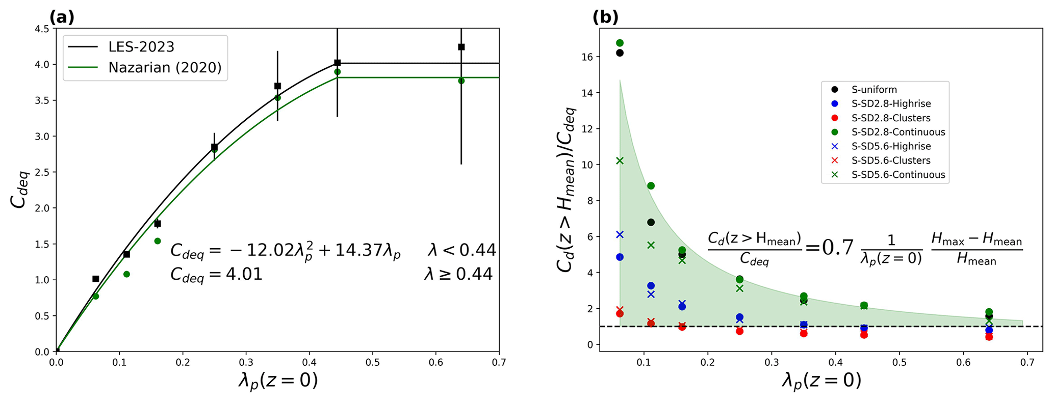
Figure 7 Drag parameterization based on the equivalent drag coefficient C_deq. Panel (a) shows the error bar plot where black squares mark the binned value of C_deq among seven building height configurations, and the vertical line attached to each square indicates the standard deviation for each bin. The green dots indicate C_deq evaluated over uniform-staggered cases from Nazarian et al. (2020). Panel (b) shows the scatter plot of the ratio between C_deq and the drag coefficient evaluated above the mean building height where the dashed line indicates the ratio of 1. The green-shaded area indicates the corresponding parameterization in the plot.

Accordingly, characterizing drag impacts converts to evaluating the drag coefficient C_d that comes in different forms in the literature (e.g., Santiago et al., 2013). The equivalent drag coefficient C_deq evaluated following Santiago and Martilli (2010b) requires fewer inputs but maintains a similar performance, as demonstrated by its capacity in MLUCM v2.0 (Nazarian et al., 2020). It will be retained in the present study. Using C_deq for the evaluation assumes a constant profile of drag that ensures the integral of the drag over the whole urban canopy is equivalent to that evaluated from LES simulations:

$$\begin{array}{}\text{(14)}& C_{\mathrm{deq}}={\displaystyle \frac{\frac{-\mathrm{1}}{\mathit{\rho }H}{\int }_{\mathrm{0}}^H\mathrm{\Delta }\langle \stackrel{\mathrm{‾}}{p\left(z\right)}\rangle \mathrm{d}z}{\frac{\mathrm{1}}{H}{\int }_{\mathrm{0}}^H\langle \stackrel{\mathrm{‾}}{u\left(z\right)}\rangle |\langle \stackrel{\mathrm{‾}}{u\left(z\right)}\rangle |\mathrm{d}z}},\end{array}$$

where $\mathrm{\Delta }\langle \stackrel{\mathrm{‾}}{p\left(z\right)}\rangle =p_{\mathrm{f}}\left(z\right)-p_{\mathrm{b}}\left(z\right)$ is the pressure deficit between the windward and leeward facets of each building block. Due to the low variance of C_deq over the impact of height variability except for denser layouts λ_p≥0.35, we binned all seven cases over each density in Table 2 to show their mean and standard deviation in Fig. 7 together with that from Nazarian et al. (2020) for uniform-staggered arrays. The excellent agreement with C_deq in the present study indicates the parameterization in Nazarian et al. (2020) presents great resilience to the height variability, especially over the sparse layouts. Therefore, updating the constants in the original parameterization requires only a minor change. However, height variability not only extends the vertical range of the urban canopy but also complicates the vertical structure of the drag coefficient and requires extra characterization. Figure 7b shows the ratio between the drag coefficient above the mean building height H_mean and C_deq that covers a range that is generally larger than unity and shows a decreasing trend with densities, which can be captured by considering the morphological condition of the urban surface from Lu et al. (2023a).

The last term parameterized is the dissipation length scale from Eq. (5). As indicated in the left panel of Fig. 8, the impact of height variability $l_{\mathit{\epsilon }}/C_{\mathit{\epsilon }}$ below the mean building height only demonstrates a very minor variation for each density range. The variation is more evident above H_mean, with a clear shape following the sectional density, and was discussed in Lu et al. (2023a). Despite the fact that applying a sophisticated dissipation and drag parameterization might lead to better model performance (Glazunov et al., 2021; Castro, 2017; Sützl et al., 2021a), it is beyond the scope of the present study, which is focused on refining the transport characterization of UCM. Therefore, we decided to keep the original parameterization from MLUCM v2.0 (Nazarian et al., 2020). For completeness, we briefly describe the parameterization strategy: by segmenting the urban canopy flow into the mixing layer, transition region, and wall-bounded layer (Coceal and Belcher, 2004), the parameterization reads

$$\begin{array}{}\text{(15a)}& {\displaystyle }& {\displaystyle }{l}_{\mathit{\epsilon }}/C_{\mathit{\epsilon }}={\mathit{\alpha }}_{\mathrm{1}}(H_{\mathrm{mean}}-d)& {\displaystyle }z/H_{\mathrm{mean}}<\mathrm{1},\text{(15b)}& {\displaystyle }& {\displaystyle }{l}_{\mathit{\epsilon }}/C_{\mathit{\epsilon }}={\mathit{\alpha }}_{\mathrm{1}}(z-d)& {\displaystyle }\mathrm{1}\le z/H_{\mathrm{mean}}\le \mathrm{1.5},\text{(15c)}& {\displaystyle }& {\displaystyle }{l}_{\mathit{\epsilon }}/C_{\mathit{\epsilon }}={\mathit{\alpha }}_{\mathrm{2}}\left(z-d_{\mathrm{2}}\right)& {\displaystyle }z/H_{\mathrm{mean}}>\mathrm{1.5},\end{array}$$

where α₁=5.5 is a revised value based on 49 simulations in the present study, and $d=H_{\mathrm{mean}}{\mathit{\lambda }}_p^{\mathrm{0.15}}$ is the displacement height parameterized following Krayenhoff et al. (2015). Equation (15a) depicts a mixing layer type of flow with a constant dissipation efficiency and Eq. (15b) represents the transition to a fully wall-bounded flow in Eq. (15c) where the dissipation efficiency decreases with height based on d₂ and α₂ parameterized as follows:

$$\begin{array}{}\text{(16a)}& {\displaystyle }& {\displaystyle }{\mathit{\alpha }}_{\mathrm{2}}\left({\mathit{\lambda }}_p\right)=min\left(\mathrm{5},max\left(\mathrm{2},\mathrm{1.3}{\mathit{\lambda }}_p^{-\mathrm{0.45}}\right)\right)\text{(16b)}& {\displaystyle }& {\displaystyle }{d}_{\mathrm{2}}\left({\mathit{\lambda }}_p\right)=\mathrm{1.5}H\left(\mathrm{1}-{\displaystyle \frac{{\mathit{\alpha }}_{\mathrm{1}}}{{\mathit{\alpha }}_{\mathrm{2}}}}\right)+\mathrm{d}\left({\mathit{\lambda }}_p\right){\displaystyle \frac{{\mathit{\alpha }}_{\mathrm{1}}}{{\mathit{\alpha }}_{\mathrm{2}}}}.\end{array}$$

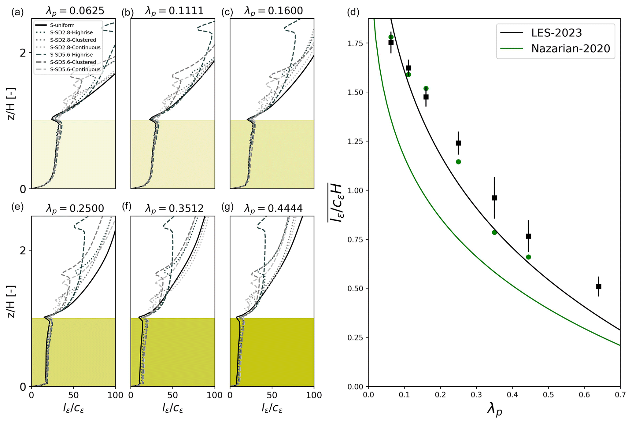
Figure 8 The left panels ((a)–(c),  (e)–(g)) show the vertical profiles of dissipation length scales $l_{\mathit{\epsilon }}/C_{\mathit{\epsilon }}$ up to 2.5H_mean where the yellow-shaded range indicates mean building height. The right panel (d) shows the binned vertical averaged dissipation length scale $\stackrel{\mathrm{‾}}{l_{\mathit{\epsilon }}/C_{\mathit{\epsilon }}}$ in the same manner as Fig. 7 overlaid with the parameterization and with that from Nazarian et al. (2020).

4 MLUCM performance with updated parameterizations

In this section, we evaluate the predictability of two modifications to the original MLUCM developed in Nazarian et al. (2020), where the combination of changes proposed in Sects. 3.1 and 3.2 and the original model form four scenarios, as shown in Table 2.

Table 2 Four scenarios tested in the present study with the combination of the EDMF approach (Sect. 3.2) and differentiation in the TKE diffusion (Sect. 3.1 ). Here, 1D-Original aims to set a baseline by employing a similar parameterization from Nazarian et al. (2020) with an adaptation for the height variability from Sect. 3.3. Therefore, the 1D-Original does not differentiate turbulent TKE flux from turbulent momentum flux and lumps the dispersive momentum flux into the calculation of K_m (To K_m). 1D-K_k considers the differentiation of TKE transport from momentum as discussed in Sect. 3.1. By contrast, 1D-EDMF only considers the “EDMF” parameterization for dispersive momentum flux while 1D-K_kEDMF considers both modifications. The bold font in the table indicates modified components from the original MLUCM.

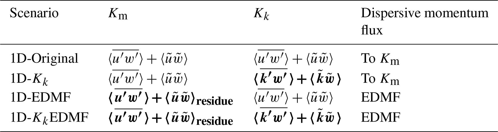
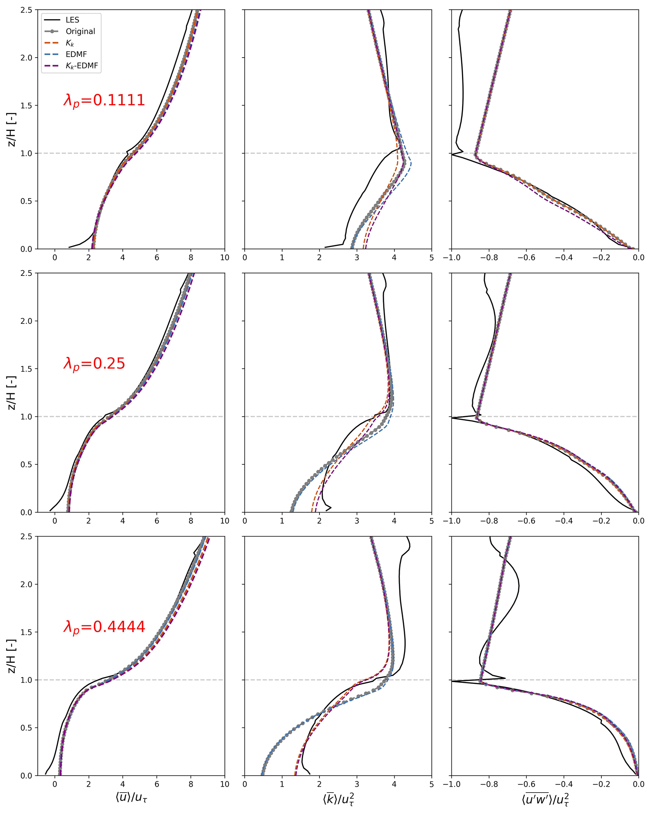
Figure 9 Vertical profiles of velocity ($\langle \stackrel{\mathrm{‾}}{u}\rangle /u_{\mathit{\tau }}$), turbulent kinetic energy ($\langle \stackrel{\mathrm{‾}}{k}\rangle /u_{\mathit{\tau }}^{\mathrm{2}}$), and turbulent momentum flux ($\langle \stackrel{\mathrm{‾}}{u^{\prime }{w}^{\prime }}\rangle /u_{\mathit{\tau }}^{\mathrm{2}}$) obtained with the four scenarios in Table 2 and LES results for sparse (λ_p=0.1111), medium (λ_p=0.25), and dense (λ_p=0.4444) layouts.

Figure 9 shows the vertical profiles of horizontally averaged velocity, TKE, and turbulent momentum flux calculated with the one-dimensional models with different transport characterization and compared with the corresponding LES results for the high-rise configuration with H_std=5.6 m. The profile comparison for other configurations can be found in the Supplement. We select sparse (λ_p=0.1111), medium (λ_p=0.25), and dense (λ_p=0.4444) layouts to reflect different flow regimes for comparison.

The prediction of streamwise velocity does not present a great variation, where 1D-K_k-EDMF exhibits the highest value. This is explained by the newly introduced mass-flux term as an explicit source of momentum and differentiation of K_k from K_m enhancing the momentum transport from the atmosphere to the canopy.

For TKE estimation, 1D-K_k and 1DK_k-EDMF with differentiation of K_k from K_m (Table 2) demonstrate a significant improvement on the TKE profile for medium and dense layouts below H_mean. The introduction of EDMF is phenomenologically equivalent to imposing a stronger pressure gradient, which leads to higher velocity and explains the better agreement with LES for the 1D-EDMF and 1D-K_k-EDMF scenarios. As a result, 1D-K_k-EDMF yields an even higher TKE due to the introduction of a mass-flux term to parameterize dispersive momentum flux as an explicit source leading to higher TKE production. The correction of TKE not only leads to better modeling of the velocity profile but also enhances the prediction of urban fluxes such as the overestimation of daytime air temperature by correcting the vertical exchange of heat (Krayenhoff, 2014).

The variation in the performance of scenarios is not pronounced across different height variability, which further consolidates the binning strategy for parameterization in the present study. To evaluate the comprehensive performance of scenarios over different height configurations, Fig. 10 presents the root mean square error (RMSE) between vertical profiles (ranging from $z=[\mathrm{0}-\mathrm{3}{H}_{\mathrm{mean}}]$) of LES and four MLUCM scenarios averaged over seven configurations (one uniform and six variable height, as shown in Table 1) over seven densities.

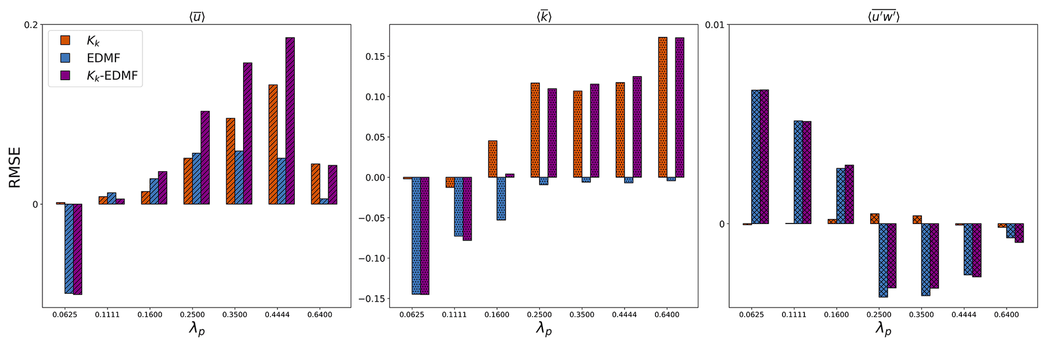
Figure 10 Difference in the root mean square error (RMSE) between the original MLUCM v2.0 (original) and three improved scenarios (positive values indicate better performance from scenarios). The RMSE is evaluated between the one-dimensional model from Table 2 against LES across seven densities in combination with seven height configurations from Table 1. Each column shows the averaged RMSE difference across seven height configurations.

The new parameterizations with refined transport characterization represent an overall improvement over the previous multi-layer model (Nazarian et al., 2020). All three scenarios with modifications lead to better predictability for velocity except for the two sparse layouts. The predictability for TKE is substantially better from the 1D-K_k and 1D-K_kEDMF scenarios, except for two sparse layouts that can be further improved with a better characterization of the TKE budget terms such as dissipation and wake production (Blunn et al., 2022). The turbulent momentum flux is diagnostically obtained in MLUCM based on the k−l closure ($\langle \stackrel{\mathrm{‾}}{u^{\prime }{w}^{\prime }}\rangle =-C_k{l}_k\langle \stackrel{\mathrm{‾}}{k}{\rangle }^{\mathrm{1}/\mathrm{2}}\frac{\partial 〈\stackrel{\mathrm{‾}}{u}〉}{\partial z}$) that is highly related to streamwise velocity and TKE. However, it exhibits a consistently contrasting performance trend compared to TKE, which leads to less improvement in denser layouts. This pattern can be attributed to both improvements (Table 2) enhancing the vertical exchange of flow properties within the canopy, which results in a smaller vertical gradient of streamwise velocity. Having the most remarkable performance, 1D-K_kEDMF with both modifications from Sects. 3.1 and 3.2 is desirable for MLUCM v3.0.

5 Summary and conclusions

This study refined the characterization of the transport of flow properties for the multi-layer urban canopy model via a separate parameterization of TKE diffusion and introduced a “mass-flux” term for the dispersive transport of momentum. The updated multi-layer model demonstrates an improved performance by correcting the underestimation of turbulent exchange and velocity below the mean building height H_mean.

By analyzing 49 LES simulations over staggered urban arrays of uniform and variable building height and comprehensive density coverage, we found the turbulent exchange rate of momentum is similar to that for scalars but 3.5 times lower than TKE. However, the previous model (MLUCM v2.0, Nazarian et al., 2020) assumed a unified transport efficiency for momentum and TKE, which curbs the transport of the flow above H_mean into the canopy and causes an underestimation of in-canopy TKE and wind speed. The accurate characterization of TKE transport into the lower canopy becomes critical as it also controls the turbulent exchange of heat and moisture between buildings and vegetation.

Regarding applications, the enhanced model, which addresses the underprediction of in-canopy TKE, has the potential to alleviate the overestimation of daytime air temperature and diurnal temperature range (Krayenhoff et al., 2020). Furthermore, the improved prediction of urban fluxes reinforces the advantages of MLUCM over simpler bulk schemes, emphasizing their ability to realistically simulate vertical diffusion processes in mesoscale atmospheric models (Hendricks et al., 2020). The proposed refinements are not exclusively constrained to urban applications but are also applicable to broader turbulence modeling. For example, the explicit parameterization of dispersive momentum flux could benefit turbulence modeling over other types of roughness elements such as coral reefs (Davis et al., 2021) and vegetative canopies (Finnigan, 2000). In parallel, emphasizing the distinction between TKE transport efficiency and its momentum counterpart underscores the importance of gathering higher flow moments for modeling general atmospheric flow (Ghonima et al., 2017).

We also revealed the distinct horizontal distribution of dispersive momentum flux, which is induced by flow heterogeneity responding to windward (quadrant 3, upward), lateral (quadrant 4, downward), and leeward (quadrant 2, downward) flow patterns. In response to this complication, we applied a sampling filter to the cumulative density function of the dispersive transport to segment the building-induced contribution (MF) that scales well with the pressure gradient and the rest of the relatively undisturbed component that can be securely lumped into the turbulent counterpart in the 1.5-order turbulent closure (ED). The EDMF framework, having successfully modeled the planetary boundary layer with flow heterogeneity induced by thermal effects, was demonstrated to be also favorable for the representation of flow heterogeneity caused by rigid building volumes. The new framework enables an explicit consideration of the impact of flow heterogeneity in MLUCM, improving our ability to calibrate the model for simulations of complex canopy flow.

With adaptations to the parameterizations of drag coefficient and dissipation length scale to account for building height variability, the model configuration that includes both the updated eddy diffusivity of TKE (K_k) and the EDMF scheme yields an improved performance relative to MLUCM v2.0. However, analysis of the flow profiles and length scales indicates future investigation is needed to address the following aspects:

1. The turbulent length scales show a great variance over heights for layouts with non-uniform building height. A height-dependent parameterization of turbulent length scale and drag profile is necessary to correctly simulate features of urban flow such as the logarithmic or exponential behavior of the wind speed profile (Castro, 2017).

2. The dispersive transport of TKE and scalars can be considered similarly following the dispersive momentum flux parameterization. In the original implementation of EDMF in PBL parameterizations (Siebesma et al., 2007), the sampled air parcel also exchanges flow properties with the turbulent environment and other air parcels, which could be considered in future developments.

3. Staggered building arrays were found to be less representative of flow over realistic dense urban neighborhoods (Lu et al., 2023b). The wind direction (Santiago et al., 2013) and thermal effects (Simón-moral et al., 2016) also affect dynamic urban flow parameterizations. Further simulation for model calibration should account for these factors for a more realistic flow characterization.

4. Similar to the scarcity of evaluations of the eddy diffusivity of flow properties other than momentum, the variation of the TKE budget terms is still poorly considered in urban flow models. Accordingly, a more comprehensive analysis that addresses the relationships between the urban morphology and the TKE budget may provide further improvements.

5. The applicability of the 1.5-order k−l turbulence closure in MLUCM is restricted to isotropic turbulence flow, where the momentum exchange rate is directly correlated with turbulence strength. However, this scaling becomes questionable even in neutral conditions and diminishes under thermal stratification, where turbulence tends to be highly anisotropic (Stiperski and Calaf, 2018). In response to these limitations, employing a higher-order closure that diagnostically assesses momentum transfer (Wilson, 1988; Ayotte et al., 1999) or considering alternative scaling approaches for poorly performing regions (Sun et al., 2020) may contribute to the development of more effective urban canopy models in the future.

Appendix A: Sampling of the dispersive momentum flux

The sampling procedure to extract the components of building-induced dispersive fluxes was conducted as follows: (a) separating the dispersive fluxes into gradient (downward) and counter-gradient (upward) components, (b) sorting these two fluxes into a descending order in terms of the magnitude, (c) lowering the cumulative density function of the two fluxes from the largest allows a smaller subdomain to be sampled until subdomains only enclose transport events connected to buildings, and (d) spatially averaging the sampled dispersive fluxes over subdomains for both gradient and counter-gradient dispersive momentum flux. Figure A1 shows a range of cut-off values ($\mathrm{co}\in [\mathrm{0.3},\mathrm{0.4},\mathrm{0.5},\mathrm{0.6},\mathrm{0.7}]$) for CDF over an example for λ_p=0.25. The cut-off value here is determined as 0.5 for all cases considered (an example is provided in Fig. 4b, where blue (red) lines enclose the sampled downward (upward) transports).

The three-dimensional distribution of the sampled dispersive structures is shown in Fig. A2 S-highrise-SD56 for ${\mathit{\lambda }}_p\in [\mathrm{0.0625},\mathrm{0.4444}]$ where the dispersive momentum flux concentrates in the immediate vicinity downstream of the cubes. Structures near the ground contributed significantly to negative stresses (green structures) where the recirculating flows dominate. In response to this distribution (note the dispersive velocity vectors in Fig. 4d), the parameterization for the vertical variation of sampled dispersive fluxes is stronger over the lower part of the canopy over sparse layouts, which is in general agreement with Poggi and Katul (2008a). In the upper levels of the canopy, the counter-gradient stresses (red structures) are more pronounced at the windward facets due to flow reflection.

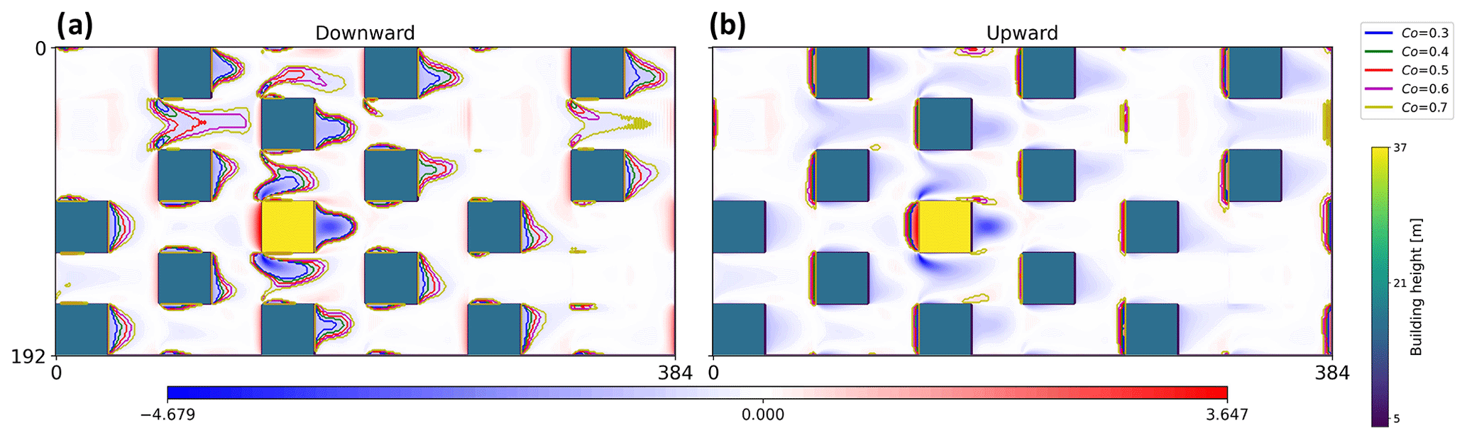
Figure A1 Sampling regions of dispersive fluxes for five ($\mathrm{co}\in [\mathrm{0.3},\mathrm{0.4},\mathrm{0.5},\mathrm{0.6},\mathrm{0.7}]$) cut-off CDF values as discussed in Sect. 3.2. Higher cut-off values for CDF lead to broader sampling regions and lower mean strength in the mass-flux term.

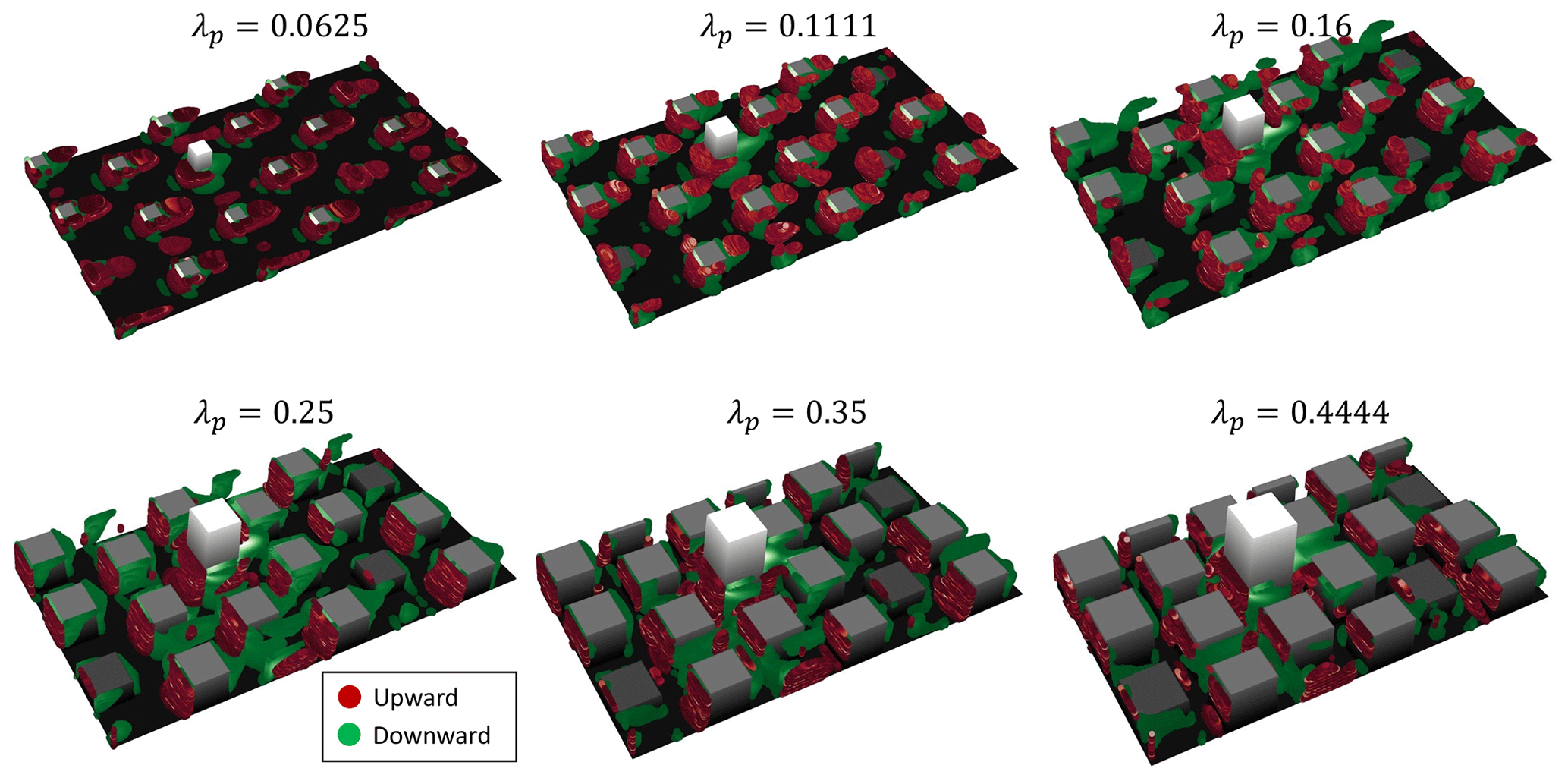
Figure A2 Three-dimensional distribution of the dispersive coherent structures for cases with S-highrise-SD56 covering ${\mathit{\lambda }}_p\in [\mathrm{0.0625},\mathrm{0.4444}]$. Green and red regions represent gradients and counter-gradient dispersive transport sampled with a 50 % CDF.