A new temperature–photoperiod coupled phenology module in LPJ-GUESS model v4.1: optimizing estimation of terrestrial carbon and water processes

Vegetation phenological shifts impact the terrestrial carbon and water cycle and affect the local climate system through biophysical and biochemical processes. Dynamic global vegetation models (DGVMs), serving as pivotal simulation tools for investigating climate impacts on terrestrial ecosystem processes, incorporate representations of vegetation phenological processes. Nevertheless, it is still a challenge to achieve an accurate simulation of vegetation phenology in the DGVMs. Here, we developed and implemented spring and autumn phenology algorithms into one of the DGVMs, LPJ-GUESS. The new phenology modules are driven by temperature and photoperiod and are parameterized for deciduous trees and shrubs by using remotely sensed phenological observations and the reanalysis data from ERA5. The results show that the LPJ-GUESS with the new phenology modules substantially improved the accuracy in capturing the start and end dates of growing seasons. For the start of the growing season, the simulated RMSE for deciduous trees and shrubs decreased by 8.04 and 17.34 d, respectively. For the autumn phenology, the simulated RMSE for deciduous trees and shrubs decreased by 22.61 and 17.60 d, respectively. Interestingly, we have also found that differences in the simulated start and end of the growing season also alter the simulated ecological niches and competitive relationships among different plant functional types (PFTs) and subsequentially influence the terrestrial carbon and water cycles. Hence, our study highlights the importance of accurate phenology estimation to reduce the uncertainties in plant distribution and terrestrial carbon and water cycling.

1 Introduction

Vegetation plays a pivotal role within the terrestrial ecosystem as the interplay between vegetation and climate exerts significant influence on the mass and energy cycles across a broad range of temporal and spatial scales (Zhu et al., 2016; Piao et al., 2019; Chen et al., 2022a). In recent years, with the increase in carbon dioxide concentration and land surface temperature, significant vegetation greening has been reported worldwide, and the annual growth dynamics of vegetation have undergone significant changes, especially the spring and autumn phenological changes (Zhu et al., 2016). A large amount of research evidence has indicated that climate change results in the advancement of spring phenology and the postponement of autumn phenology, exerting a profound influence on the carbon and water cycles within terrestrial ecosystems (Piao et al., 2019; Badeck et al., 2004; Zhou et al., 2020) and the geographic distribution of species (Chuine, 2010; Fang and Lechowicz, 2006; Huang et al., 2017). Under conditions of sufficient water supply and no radiation constraints, the extension of the growing season resulting from vegetation phenological shifts will contribute additional carbon sinks to terrestrial ecosystems (Zhang et al., 2020; Keenan et al., 2014). Longer growing seasons also lead to greater evapotranspiration, mainly in early spring and autumn, which in turn reduces watershed runoff (Huang et al., 2017; Kim et al., 2018; Chen et al., 2022b; Geng et al., 2020). Nevertheless, it is still a challenge to achieve an accurate simulation of vegetation phenology in dynamic global vegetation models (DGVMs), especially in the context of climate change (Richardson et al., 2012). We urgingly caution that improving the vegetation phenology module of DGVMs and taking the response of vegetation phenology to climate change into consideration is a necessary development to improve model simulation accuracy and reduce model uncertainty.

The DGVMs generally include phenology modules in vegetation submodels, but the implementations vary widely, which include the following:

1. Fixed and prescribed seasonal dynamics are used to characterize phenology, and the models using this method include the SiB model, SiBCASA model, and ISAM (Sellers et al., 1986; Schaefer et al., 2008; Jain and Yang, 2005).

2. Remote sensing data or in situ observations directly describe the vegetation growth dynamics instead of the process-based simulation, and SiB2, BEPS, and ED2 are all based on this method to describe the vegetation growth dynamics (Sellers et al., 1996; Deng et al., 2006; Medvigy et al., 2009).

3. The vegetation phenology algorithm is used, which takes the response of vegetation biophysiology to environment factors into account to simulate vegetation growth dynamics.

In comparison to the first two methods, the third approach offers the advantage of depicting the responses of vegetation to the external environment grounded in a plant physiological process and can trace the dynamics of vegetation growth amidst changing environmental conditions, so it is adopted by several DGVMs, e.g., Biome-BGC, ORCHIDEE, and LPJ-GUESS (Thornton et al., 2002; Krinner et al., 2005; Sitch et al., 2003). With the evolving comprehension of the intricate response mechanisms of vegetation to external environment, vegetation phenological algorithms have experienced substantial advancements in recent decades, which encompass shifts from single-process to multi-process mechanisms and from single-variable to multi-factor model constraints (Liu et al., 2018a; Fu et al., 2020; Piao et al., 2019). For spring phenological algorithms, in the early stage, temperature was the only factor considered, resulting in relatively simplistic model processes, which were also commonly adopted by DGVMs (growing degree days, or GDD, and Unified, etc.; Sarvas, 1972; Chuine, 2000). With deepening understanding of spring phenological mechanisms, factors such as radiation and photoperiod have been introduced into the phenological algorithm, and the corresponding complex regulatory mechanisms have also been perfected, e.g., sequential algorithm, parallel algorithm, and DORMPHOT algorithm (Hänninen, 1990; Kramer, 1994; Caffarra et al., 2011). As for the autumn phenological algorithm, the early algorithm form was also relatively simple (a cold temperature-driven CDD algorithm) but widely used in DGVMs, and some DGVMs used a fixed leaf longevity for the determination of autumn phenological dates. The development of relatively complex autumn phenological mechanism algorithms is relatively late, and these advanced autumn phenological algorithms take photoperiod and carbon accumulation into account in the algorithm process, such as the temperature-photoperiod bioclimatic (DM) algorithm and the photosynthesis-influenced autumn phenology (PIA) algorithm (Zani et al., 2020; Delpierre et al., 2009). Many studies have pointed out that early phenological algorithms tend to be overly simplistic and result in biased predictions, which indicates that the vegetation phenological algorithms of DGVMs need to be updated urgently (Kucharik et al., 2006; Ryu et al., 2008). The use of more accurate phenological algorithms covering more complex mechanisms is of great significance in reducing the simulation errors in DGVMs and improving the simulation reliability under future climate warming.

In this study, we used the remote-sensing-based phenology data and the threshold and maximum change rate methods to parameterize the spring DORMPHOT algorithm and autumn DM algorithm. This was explicitly applied for the boreal needleleaved summergreen tree (BNS), shade-intolerant broadleaved summergreen tree (IBS), shade-tolerant temperature broadleaved summergreen tree (TeBS), and summergreen shrub plant function types (PFTs). The new phenology module with these parameters was coupled into the LPJ-GUESS model. The objectives of this study are as follows: (1) to couple more mechanistic phenology modules into the LPJ-GUESS model to improve the accuracy of spring and autumn phenology simulations and (2) to assess the impacts of different vegetation phenological algorithms on the carbon and water process simulations.

2 Materials and methods

2.1 Datasets

2.1.1 GIMMS NDVI_4g

The normalized differential vegetation index (NDVI) is commonly used as a proxy for vegetation canopy greenness and growth condition. In the study, we used the fourth-generation NDVI dataset of GIMMS, which provides biweekly NDVI records with a spatial resolution of $\mathrm{1}/\mathrm{12}$° (∼ 8 km) during 1982–2017 to extract the start and end of the growing season (Pinzon and Tucker, 2014; Tucker et al., 2005; Cao et al., 2023). This NDVI dataset has been refined and corrected for orbital drift, calibration, viewing geometry, and volcanic aerosols, which can accurately reflect the accurate growth dynamics of surface vegetation (Kaufmann et al., 2000).

2.1.2 Climate forcing field data

We used CRU-NCEP V7 data with a horizontal spatial resolution of 0.5 × 0.5° as the forcing field data for driving the LPJ-GUESS model during 1901–2015. The forcing field data include monthly air temperature (1901–1978) and precipitation, wind speed, wet days, incoming shortwave radiation, and relative humidity measurements over the period 1901–2015, which can be downloaded from https://rda.ucar.edu/datasets/ds314.3/ (last access: 28 March 2024​​​​​​​). The ERA5-Land daily air temperature dataset has been used to parameterize spring and autumn phenological algorithms and force the LPJ-GUESS model. The dataset is a global reanalysis dataset developed by the European Centre for Medium-Range Weather Forecasts (ECMWF), which utilizes advanced data assimilation techniques by combining observations from various sources, such as satellites, weather stations, and weather balloons, with numerical weather prediction models. We downloaded the ERA5-Land and daily air temperature at a 0.5° spatial resolution (consistent with the CRU NCEP V7 data from 1979–2015) from their official website (https://cds.climate.copernicus.eu/apps/user-apps/app-c3s-daily-era5-statistics; last access: 28 March 2024). Due to a possible bias between different datasets, we calculated the monthly average of the ERA5-Land daily air temperature and calculated its climatology as well as the climatology of the CRU NCEP V7 monthly air temperature data, and we corrected the bias of the ERA5-Land data according to the deviation.

2.1.3 GLC2000 land cover data

Satellite remote sensing can capture the collective information from mixed pixels comprised of various plants and also information from dominant vegetation. The data acquired through satellite remote sensing can be regarded as representative of a particular vegetation type only when the plant functional types within a grid cell exhibit a relatively homogeneous composition. Based on the GLC2000 land cover types data, which are designated according to PFTs ascribed to satellite images and ground truth by regional analysts with a 1 km spatial resolution (Bartholome and Belward, 2005), we calculated the proportion of different PFTs in the 0.5 × 0.5° grid cell to identify pixels dominated by a specific plant functional type (the proportion of a specific plant function type is greater than 50 %; Figs. 1 and S1).

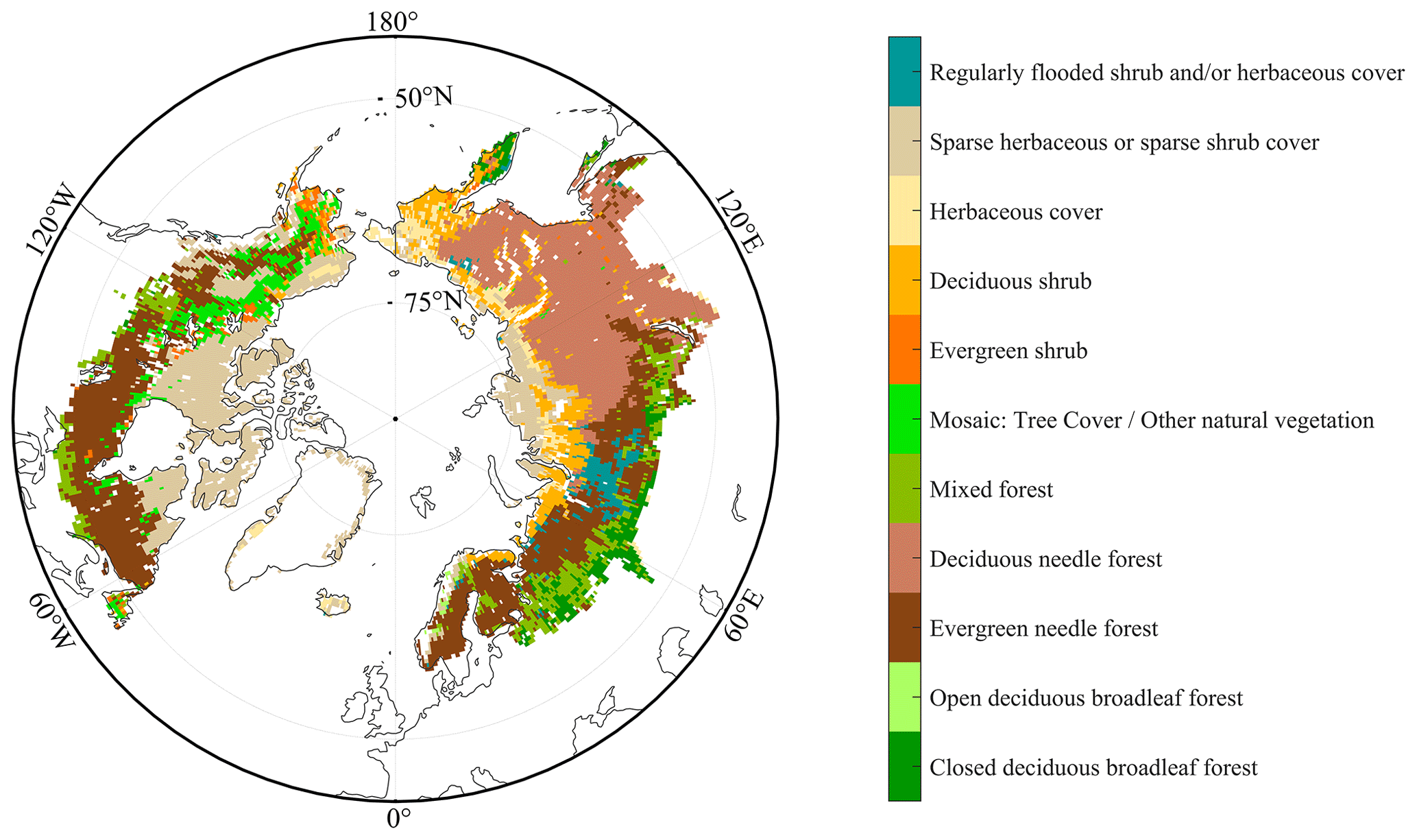
Figure 1 The spatial distributions of 11 detailed regional land cover types in the GLC2000 products. BNS (boreal needleleaved summergreen tree): deciduous needle forest. IBS–TeBS trees (shade-intolerant broadleaved summergreen tree and shade-tolerant temperate broadleaved summergreen tree): open deciduous broadleaf forest and closed deciduous broadleaf forest. Shrubs (summergreen shrubs): sparse herbaceous or sparse shrub cover and deciduous shrubs.

2.1.4 VPM GPP and REA ET data

We used the vegetation photosynthesis model (VPM) gross primary productivity (GPP) (Zhang et al., 2017a) and REA ET (reliability ensemble averaging; Lu et al., 2021a) to compare the simulation results of carbon and water fluxes with the LPJ-GUESS model.

The VPM GPP dataset is constructed upon an enhanced light use efficiency theory, utilizing satellite data from MODIS and climate data from NCEP Reanalysis II. It incorporates an advanced vegetation index (VI) gap-filling and smoothing algorithm, along with distinct considerations for C₃/C₄ photosynthesis pathways. The VPM GPP product can be downloaded from https://doi.org/10.6084/m9.figshare.c.3789814.v1 (Zhang et al., 2017​​​​​​​b).

REA ET is a combination of three existing model-based products: the fifth-generation ECMWF reanalysis (ERA5), the Global Land Data Assimilation System Version 2 (GLDAS2), and the second Modern-Era Retrospective analysis for Research and Applications (MERRA-2), which uses the reliability ensemble averaging (REA) method, minimizing errors using reference data, to combine the three products over regions with high consistencies between the products using the coefficient of variation (CV). The REA ET data can be accessed at https://doi.org/10.5281/zenodo.4595941 (Lu et al., 2021a, b).

2.2 Phenology dates extraction

We used five phenological extraction methods, which include three threshold-based methods (i.e., Gaussian midpoint, spline midpoint, and TIMESAT-SG methods) and two change-rate-based methods (i.e., the HANTS maximum and polyfit maximum methods), following previous studies (Cong et al., 2012; Savitzky and Golay, 1964; Chen et al., 2023a), to retrieve spring (start of growing season, SOS) and autumn (end of growing season, EOS) phenological events (Fig. S2). Phenological extraction based on multiple methods consists of three steps: (1) smoothing and interpolating the NDVI date to obtain the smooth and continuous NDVI daily time series, (2) using the threshold value (0.5 for SOS and 0.2 for EOS) or the maximum rate of change to extract the vegetation phenology from each single method (Reed et al., 1994; White et al., 1997; White et al., 2009; Piao et al., 2006), and (3) averaging the phenological results obtained by different extraction methods to reduce uncertainties associated with a single method (due to the different fitting methods, interpolation methods, and threshold settings of different extraction methods; Fu et al., 2021, 2023).

2.3 Model description

LPJ-GUESS is a process-based dynamic global vegetation model that can simulate vegetation dynamics and soil biogeochemical processes across different terrestrial ecosystems. At the grid cell level, the model simulates vegetation growth, allometry competition, mortality, and disturbances (Sitch et al., 2003; Morales et al., 2005; Hickler et al., 2004). The PFTs within the framework of the LPJ-GUESS model encapsulate the extensive spectrum of structural and functional attributes that are characteristic of potential plant species. Within a given area or patch (corresponding in size approximately to the maximum area of influence of one large adult individual on its neighbors), plant growth is governed by the synergistic interplay of bioclimatic constraints and interspecific competition for spatial dominance, access to light, and vital resources. In a grid cell (stand), it is typically simulating multiple such patches to represent different disturbance histories within a landscape, and across these patches, the modeled properties tend to coalesce towards a singular, overarching average value (Smith et al., 2001).

In the LPJ-GUESS model, the spring phenology is calculated based on spring heat and winter cold requirements (Sykes et al., 1996). Plants have certain energy requirements for budburst, which are expressed by using growing degree days above 5 °C (GDD5), while growing degree days to budburst are also related to the length of the chilling period. An increase in chilling periods can reduce the requirement for growing degree days to budburst; in other words, budburst can be delayed long enough to minimize the risk that the emerging buds will be damaged by frost (Eq. 1):

$$\begin{array}{}\text{(1)}& \mathrm{GDD}=a+b\times e^{-k\times C},\end{array}$$

where a, b, and k are PFT-specific constants and C is the length of the chilling period. GDD represents the growing degree days requirement of a specific PFT at a chilling period length of C. Growing degree days are defined as the accumulation of temperatures above the base temperature (generally 5 °C), and the length of the chilling period is defined as the days that the daily mean temperature is below 5 °C.

For autumn phenology, leaf longevity was used as a threshold in the LPJ-GUESS model for the simple prediction of senescence. It is assumed in the model that autumn phenology occurs when the cumulative complete leaf longevity is greater than 210 d or the daily average temperature is below 5 °C in autumn.

Within each stand, 50 different patches (in this study) were applied to represent different disturbance histories within a landscape. The simulations over the study areas included 23 PFTs, which consist of five grass, three bryophytes, eight shrubs, and seven tree PFTs, and the summergreen PFTs involved in the improvement of the vegetation phenological simulation contain BNS, IBS, and TeBS trees and deciduous shrubs (hereafter called Shrubs); see detailed description in Tang et al. (2023) and Rinnan et al. (2020).

2.4 LPJ-GUESS phenology module extension

We improved the spring and autumn phenological modules of the LPJ-GUESS model by coupling the DORMPHOT algorithm and DM algorithm into LPJ-GUESS according to the phenological module extension flow chart (Fig. 2).

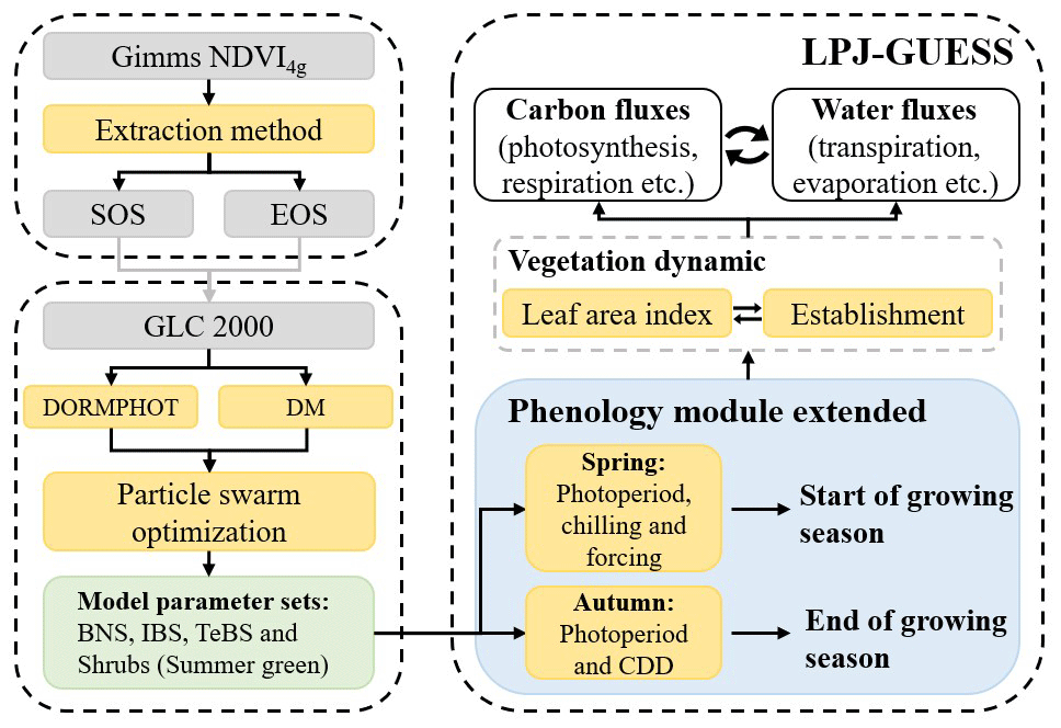
Figure 2 Flowchart of spring and autumn phenological module extension in LPJ-GUESS. Dotted boxes represent independent work, gray boxes represent different datasets or intermediate process results, and yellow boxes represent different calculation methods or model modules. CDD represents cooling degree day.

The spring phenological algorithm in LPJ-GUESS was replaced by the DORMPHOT algorithm, which introduces the effect of photoperiod on dormancy. This algorithm refines the spring phenological algorithm into three stages: dormancy induction, dormancy release, and growth resumption (Caffarra et al., 2011). The dormancy induction process is triggered by a short daily photoperiod (DR_P) and a low temperature (DR_T), and it finishes when the cumulant of the product of DR_P and DR_T reaches a specific threshold (DS >D_crit; Eqs. 2, 3, and 4):

$$\begin{array}{}\text{(2)}& {\displaystyle }\mathrm{DS}=\sum _{t_{\mathrm{0}}}^t{\mathrm{DR}}_{\mathrm{T}}\times {\mathrm{DR}}_{\mathrm{P}},\text{(3)}& {\displaystyle }{\mathrm{DR}}_{\mathrm{T}}={\displaystyle \frac{\mathrm{1}}{\mathrm{1}+e^{\mathrm{aD}\times (T-\mathrm{bD})}}},\text{(4)}& {\displaystyle }{\mathrm{DR}}_{\mathrm{P}}={\displaystyle \frac{\mathrm{1}}{\mathrm{1}+e^{\mathrm{10}\times (\mathrm{DL}-{\mathrm{DL}}_{\mathrm{crit}})}}},\end{array}$$

where t₀ is the start date of dormancy induction defined on 1 September of the year preceding budburst, DS represents the state of dormancy induction (the cumulant effect of DR_P and DR_T), T is the daily mean temperature, and DL is the day length on day t. The algorithm parameters aD, bD, and DL_crit regulate the effect of photoperiod and temperature.

Dormancy release and growth resumption start after dormancy induction is complete (t_d), which represent a parallel chilling and forcing process, respectively. The total daily rate of chilling (S_C) is defined as the accumulation of daily chilling (R_C), as seen in Eq. (5), and the daily forcing (R_f) is determined by both photoperiod and S_C (Eqs. 6, 7, and 8). The effects of photoperiod and chilling on R_f counteract each other. The increase in photoperiod will decrease R_f, while the increase in chilling will reverse the effect:

$$\begin{array}{}\text{(5)}& {\displaystyle }{S}_{\mathrm{C}}=\sum _{t_{\mathrm{d}}}^t{R}_{\mathrm{C}}=\sum _{t_{\mathrm{d}}}^t{\displaystyle \frac{\mathrm{1}}{\mathrm{1}+e^{\mathrm{aC}\times (T-\mathrm{cC}{)}^{\mathrm{2}}+(T-\mathrm{cC})}}},\text{(6)}& {\displaystyle }{\mathrm{DL}}_{\mathrm{50}}={\displaystyle \frac{\mathrm{24}}{\mathrm{1}+e^{\mathrm{hDL}\times (S_{\mathrm{C}}-C_{\mathrm{crit}})}}},\text{(7)}& {\displaystyle }{T}_{\mathrm{50}}={\displaystyle \frac{\mathrm{60}}{\mathrm{1}+e^{\mathrm{gT}\times (\mathrm{DL}-{\mathrm{DL}}_{\mathrm{50}})}}},\text{(8)}& {\displaystyle }{S}_{\mathrm{f}}=\sum _{t_{\mathrm{d}}}^t{R}_{\mathrm{f}}=\sum _{t_{\mathrm{d}}}^t{\displaystyle \frac{\mathrm{1}}{\mathrm{1}+e^{\mathrm{dF}\times (T-T_{\mathrm{50}})}}},\end{array}$$

where aC, cC, and C_crit are the algorithm parameters of the chilling process, and hDL, gT, and dF are the algorithm parameters of the forcing process. When the total daily rate of forcing (S_f) reaches a critical value F_crit, vegetation completely resumes growth and spring phenological events occur. Note that gT and hDL must be greater than zero to limit the monotonicity of Eqs. (6) and (7).

Since there is a lack of process-based submodule to simulate autumn phenology in the LPJ-GUESS model, and only a fixed leaf longevity is used to define the occurrence date of autumn phenology, we introduced an autumn phenology process that considers photoperiod and cold temperature effects by coupling the DM algorithm into the LPJ-GUESS model (Delpierre et al., 2009). The DM algorithm assumes that plants will respond to low temperature (below base temperature, T_b) only when the photoperiod is below a critical value (DL_crit), and the daily rate of senescence (R_sen) on that day is determined by a cold temperature and photoperiod (Eqs. 9, 10, and 11):

$$\begin{array}{}\text{(9)}& {\displaystyle }\begin{array}{rl}f\left(\mathrm{DL}\right)& ={\mathit{\alpha }}_{\mathrm{pn}}\times {\displaystyle \frac{\mathrm{DL}}{{\mathrm{DL}}_{\mathrm{crit}}}}+(\mathrm{1}-{\mathit{\alpha }}_{\mathrm{pn}})\times \left(\mathrm{1}-{\displaystyle \frac{\mathrm{DL}}{{\mathrm{DL}}_{\mathrm{crit}}}}\right),\\ & {\mathit{\alpha }}_{\mathrm{pn}}\in \mathit{\{}\mathrm{0},\mathrm{1}\mathit{\}}\end{array}\text{(10)}& {\displaystyle }{R}_{\mathrm{sen}}=\left\{\begin{array}{ll}\mathrm{0},& \mathrm{DL}\ge {\mathrm{DL}}_{\mathrm{crit}}\\ \mathrm{0},& \mathrm{DL}<{\mathrm{DL}}_{\mathrm{crit}}\mathrm{and}T\ge T_{\mathrm{b}}\\ (T_{\mathrm{b}}-T{)}^x\times f(\mathrm{DL}{)}^y,& \mathrm{DL}<{\mathrm{DL}}_{\mathrm{crit}}\mathrm{and}T<T_{\mathrm{b}}\end{array}\right.,\text{(11)}& {\displaystyle }{S}_{\mathrm{sen}}=\sum _{t_{\mathrm{0}}}^t{R}_{\mathrm{sen}},\end{array}$$

where α_pn is a parameter that determines that a photoperiod shorter than the DL_crit threshold weakens (α_pn equal to 1) or strengthens (α_pn equal to 0) the cold-degree sum effect. In the formula, x and y are the indices of the temperature and photoperiod terms, which are used to adjust the degree of influence of temperature and photoperiod on Rsen, respectively.

2.5 Phenological algorithm parameterization

Utilizing the spatial distribution of predominantly homogeneous pixels corresponding to distinct vegetation types, we partitioned the remote sensing phenological dataset and finally obtained the phenological dataset of BNS, IBS, and TeBS trees and Shrub PFTs for the parameterization of the DORMPHOT and DM algorithms. We divided the phenology dataset into two parts according to the odd or even number of years; the odd-numbered years represent the algorithm parameter internal calibration and the even-numbered years represent the algorithm external calibration. The particle swarm optimization (PSO) algorithm was applied to parameterize the DORMPHOT and DM algorithm for different PFTs, which used the mixed function that comprehensively considers multiple evaluation indicators as the objective function (f(mixed), Eq. 12) and sets the upper limit of iteration to 5000 times to find the global optimal parameter (Marini and Walczak, 2015; Poli et al., 2007). The parameters of the DORMPHOT algorithm and DM algorithm applicable to BNS and IBS–TeBS trees and Shrub PFTs were found by the PSO algorithm (Tables S1 and S2).

$$\begin{array}{}\text{(12)}& \begin{array}{rl}f\left(\mathrm{mixed}\right)& =\mathrm{100}\times (\mathrm{1}-R^{\mathrm{2}})+\mathrm{100}\times (\mathrm{1}-\mathrm{NSE})\\ & +\mathrm{10}\times \mathrm{RMSE},\end{array}\end{array}$$

where R² is the coefficient of determination, NSE is the Nash–Sutcliffe efficiency, and RMSE is the root mean square error. The coefficients in front of each term of the formula are used to adjust the weights of different evaluation indicators. The smaller the objective function the closer the simulated value of the algorithm is to the observed value.

2.6 Simulation setup

To compare the simulation performance of LPJ-GUESS, which employs the original phenological module and modified phenological module (the extended LPJ-GUESS), we first ran the model using CRU NCEP V7 gridded climate data over the period 1901–1978 with a 500-year spin-up, and we saved all model state variables at the end of 1978 (when we used the original phenological module, the status variables associated with the extended phenological module were also updated and saved concurrently); we avoided the differences in the simulated vegetation and soil state variables outside the study period, i.e., 1979–2015 (Viovy, 2018). Then we restarted the model simulations (applying the original phenological module and extended phenological module) with the saved model state variables at the last day of 1978 and ERA5-Land daily air temperature (note that other forcing data were still from CRU NCEP V7 dataset) and printed start (end) of growing season of summer green PFTs, monthly grid level GPP, and actual evapotranspiration (AET) of each PFT and foliage projection cover (FPC) for investigating the simulation difference which was induced by phenological simulation differences. All the data processing and analysis in this study were completed in MATLAB 2020b (https://www.mathworks.com, last access: 28 March 2024).

3 Results

3.1 Phenology simulation performance

For spring phenology, the DORMPHOT algorithm has the best simulation performance in the IBS–TeBS region (R²=0.62 and NSE = 0.62), followed by the regions dominated by BNS (R²=0.52 and NSE = 0.52) trees and Shrubs (R²=0.47 and NSE = 0.47; Table 1) PFTs. For autumn phenology, the simulation performance was generally worse than that of spring phenology. The DM algorithm has the best simulation performance in the Shrubs region (R²=0.39 and NSE = 0.39), followed by the regions dominated by BNS (R²=0.33 and NSE = 0.32) trees and IBS–TeBS (R²=0.47 and NSE = 0.47; Table 1) trees.

Table 1 Algorithm performances of the DORMPHOT and DM algorithms.

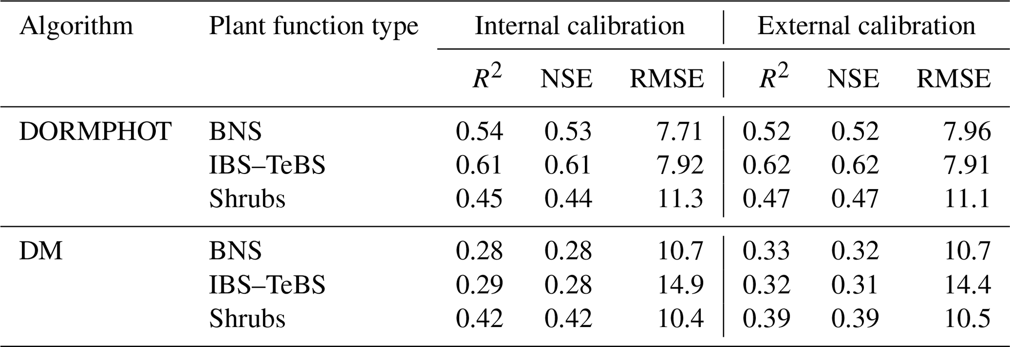
R² is the coefficient of determination, NSE is the Nash–Sutcliffe efficiency, and RMSE is the root mean square error. BNS is the boreal needleleaved summergreen tree, IBS is the shade-intolerant broadleaved summergreen tree, TeBS is the shade-tolerant temperate broadleaved summergreen tree, and Shrubs are the summergreen shrub plant function types.

Compared with the remote-sensing-based vegetation phenological indices, LPJ-GUESS, with the original phenological module, estimated an earlier spring onset and an autumn leaf senescence. The simulated spring phenology matches better than that of autumn phenology. The extended LPJ-GUESS model has greatly improved the estimation accuracy in regions dominated by BNS and IBS–TeBS trees and Shrub PFTs (Figs. 3 and S3). For spring phenology, the simulated R² (RMSE) values of the extended LPJ-GUESS model for regions dominated by BNS and IBS–TeBS trees and Shrub PFTs were 0.53 (7.84), 0.61 (7.92), and 0.46 (11.21), respectively, which increased (decreased) by 0.26 (5.55), 0.12 (17.34), and 0.25 (10.53) compared with the original phenological module.

We found that PFTs with larger R² increases in the spring phenological simulation also had smaller RMSE reductions for the extended model, indicating the improvements in capturing interannual change and the multiyear mean value. The autumn phenology simulation performance was greatly improved by integrating the DM algorithm for regions dominated by BNS and IBS–TeBS trees and Shrub PFTs, and the simulated R² (RMSE) values of the extended LPJ-GUESS model were 0.31 (10.70), 0.31 (14.69), and 0.41 (10.42), respectively, which increased (decreased) by 0.11 (15.66), 0.31 (17.60), and 0.27 (27.50). By comparing the LPJ-GUESS simulated daily leaf area index (LAI) before and after coupling the DM algorithm, we also found that the autumn LAI values simulated by the extended LPJ-GUESS no longer suddenly decreased to zero over a day but rather smoothly decreased with the sigmoid function according to the control of cold temperature and photoperiod (Fig. S4).

We also used two calibration schemes to explore the phenology simulation performance of the original phenological module of LPJ-GUESS after parameterization. The first one is based on the original LPJ-GUESS model to determine a common parameter set of all deciduous tree PFTs, and the second one is to determine a unique set of parameters for each PFTs. The results show that the phenology simulation performance of the original phenological module under the two calibration schemes was inferior to that of the new phenological module based on the cooperative control of temperature and photoperiod (Table S3)

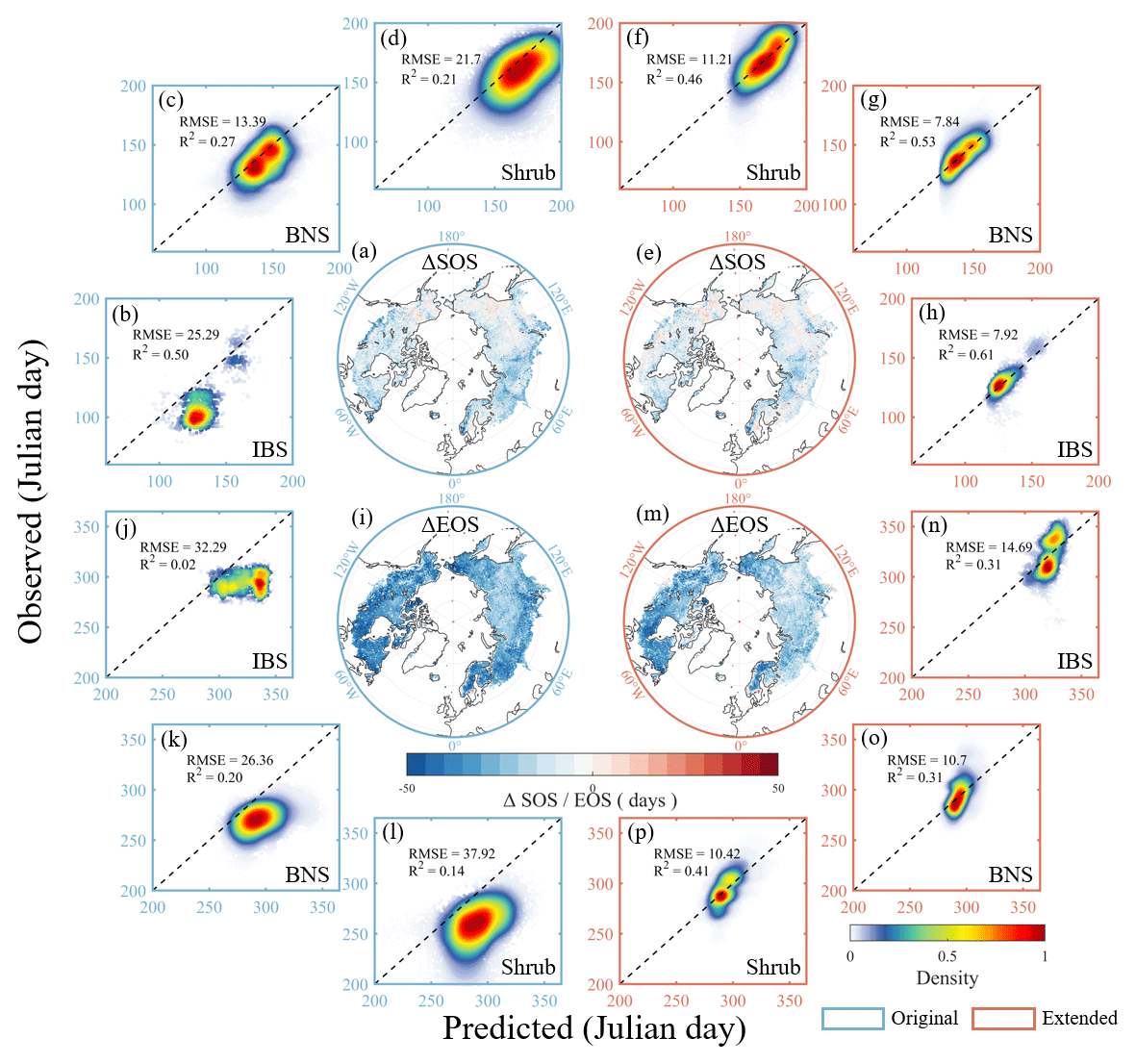
Figure 3 Comparison of the simulated performance of spring (SOS) and autumn (EOS) phenology between the original (left blue panels) and the extended (right red panels) LPJ-GUESS. (a–d) Simulation performance of SOS using the original LPJ-GUESS. (e–h) Simulation performance of SOS using the extended LPJ-GUESS. (i–l) Simulation performance of EOS using the original LPJ-GUESS. (m–p) Simulation performance of EOS using the extended LPJ-GUESS. The blue and red boxes represent spring and autumn phenological simulations. The spatial geographic map shows the difference between the simulation results of the LPJ-GUESS model and the remote sensing phenology, with blue representing the model underestimation and red representing the model overestimation. The dotted lines in the subgraph are 1:1 lines.

3.2 Gross primary productivity simulation

Since the PFTs simulated in the LPJ-GUESS model include not only BNS and IBS–TeBS trees and Shrub PFTs but also evergreen plants and grasses (no development was made to its phenological simulation in the present study), we found that clear differences between two versions of the model mainly appeared in the regions dominated by these deciduous PFTs with improved phenological modules. We only found small differences in the regions dominated by evergreen or grassland (Fig. 4c). It is also clear that the original LPJ-GUESS generally simulated higher GPP than the extended one over the study period, except for the IBS–TeBS-dominated regions, where higher GPP from the original model can only be found from 1979 to 2000 (Fig. 4d–f). By comparing multiple years' monthly mean GPP values, it becomes evident that the extended phenology also influences the seasonal dynamics of GPP. In regions dominated by BNS trees, the differences in monthly GPP are primarily noticeable during spring (using the extended phenological module resulted in a −34.9 % lower GPP in May compared to the original phenological module; when not specifically stated, the value is that the extended model differs from the original model, as can be seen in Fig. 4g). In regions dominated by IBS–TeBS trees, the GPP differs in both spring (−2.8 %) and autumn (−6.3 %), and the difference is larger in autumn, which mainly contributes to an annual GPP difference (Fig. 4h). In regions dominated by Shrub PFTs, we found differences in GPP in all months (−43.9 %), especially in the nongrowing season, indicating that some evergreen plants still exist in the region when the original phenological module is used and that changes in vegetation phenology seem to substantially affect vegetation composition in this region (Fig. 4i). Compared with VPM GPP products, we also found that LPJ-GUESS simulated GPP overestimates, but the spatial pattern is consistent with VPM GPP products, and the extended LPJ-GUESS model could simulate GPP more accurately during transition periods (Figs. S5 and S6).

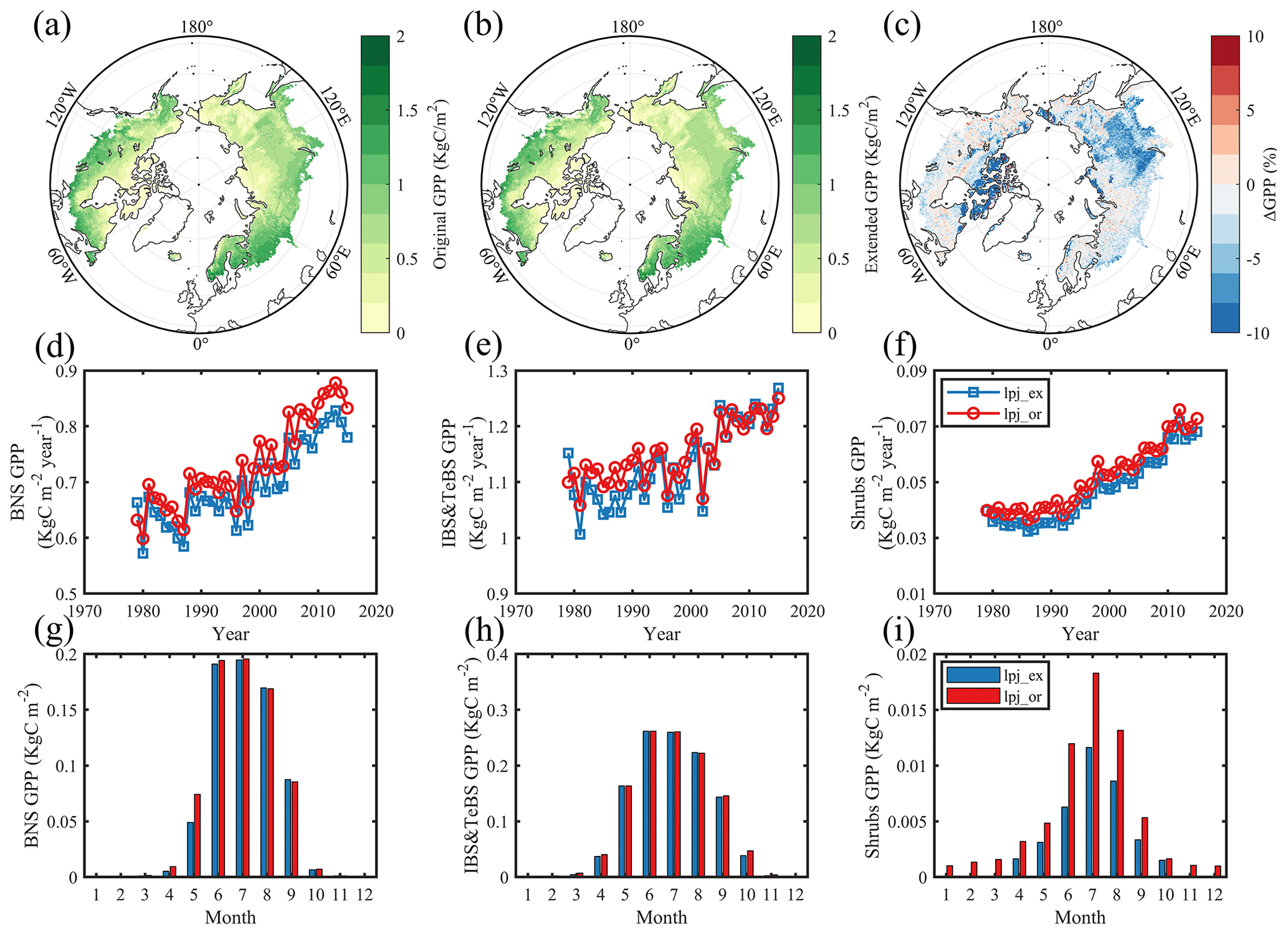
Figure 4 Comparison of gross primary productivity (GPP) simulations between scenarios which used the original phenological module and extended (DORMPHOT and DM) phenological module. (a) This scenario used the original phenological module. (b) This scenario used the extended phenological module. Panel (c) shows the difference between the two scenarios mentioned above; blue represents a larger simulation value for the LPJ-GUESS model using the original phenological module, and red represents a smaller simulation value. (d–f) Annual average GPP for BNS and IBS–TeBS trees and Shrub PFTs from 1979 to 2015. (g–i) Multiyear mean monthly GPP for BNS and IBS–TeBS trees and Shrub PFTs from 1979 to 2015.

The potential natural plant distribution also confirmed that the grid cells with large differences in phenological simulations between the original and the extended LPJ-GUESS also have large differences in dominant vegetation types (Fig. S3). We selected typical grid cells in BNS and IBS–TeBS trees and Shrubs regions and compared their multiyear variation pattern of FPC. We found that the phenological changes had a clear influence on the FPC changes in the BNS and Shrubs region (Fig. 5). However, in the IBS–TeBS region (the grid cell dominated by IBS trees was selected here), although we found that the difference in the phenological simulation affects little in FPC components due to the close proportion of IBS and BNE (boreal needleleaved evergreen) trees (fierce competition), small changes in FPC components could also lead to changes in dominant vegetation types (Fig. 5c, d).

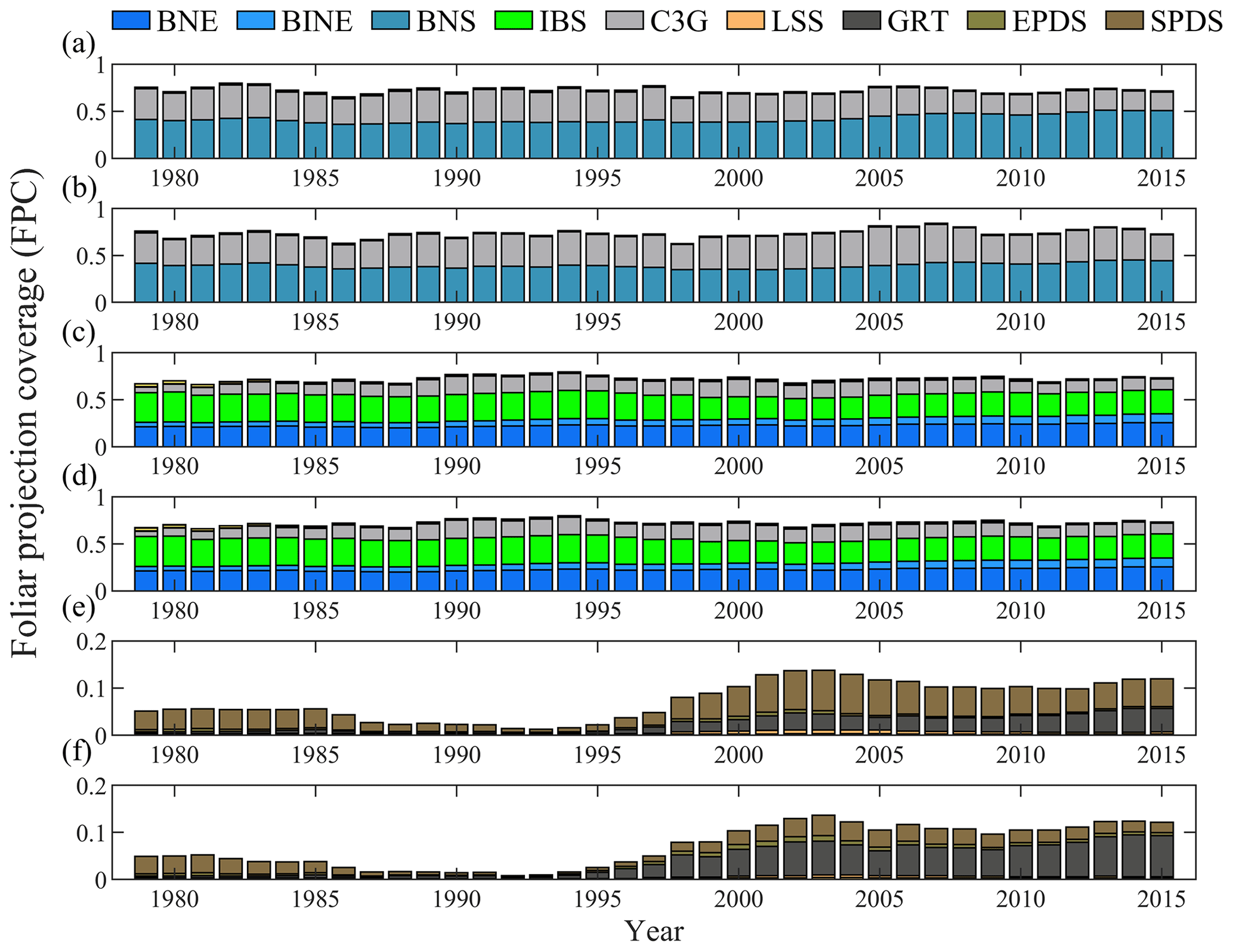
Figure 5 Shifts in foliage projection coverage (FPC) of typical grid cells in the regions dominated by BNS and IBS–TeBS trees and Shrub PFTs over the period 1979–2015. Typical grid cells of (a) BNS trees, (c) IBS–TeBS trees, and (e) Shrub PFTs that used the original LPJ-GUESS model. Typical grid cells of (b) BNS trees, (d) IBS–TeBS trees, and (f) Shrub PFTs that used the extended LPJ-GUESS model.

3.3 Evapotranspiration simulation

By comparing the spatial patterns, we found that the LPJ-GUESS-simulated AET spatial pattern is consistent with REA ET products, and BNS trees dominated the regions with large differences in the modeled AET under the two runs; the simulation result using the original phenological module was larger by 3.9 % compared with using the modified module (Figs. 6c and S7). In the IBS–TeBS-dominated region, like GPP, we found that the scenario using the original phenological module presented a larger AET during the period 1979–2000, and the two scenarios that simulated AET in the Shrub-dominated region were very close (Fig. 6e–f). The seasonal dynamic patterns of AET in regions dominated by BNS and IBS–TeBS trees and Shrub PFTs are similar. The AET simulations become higher in spring and lower in summer, and only in the Shrub-dominated region does the AET simulation become lower in autumn when the original phenology module is used (Fig. 6g–i).

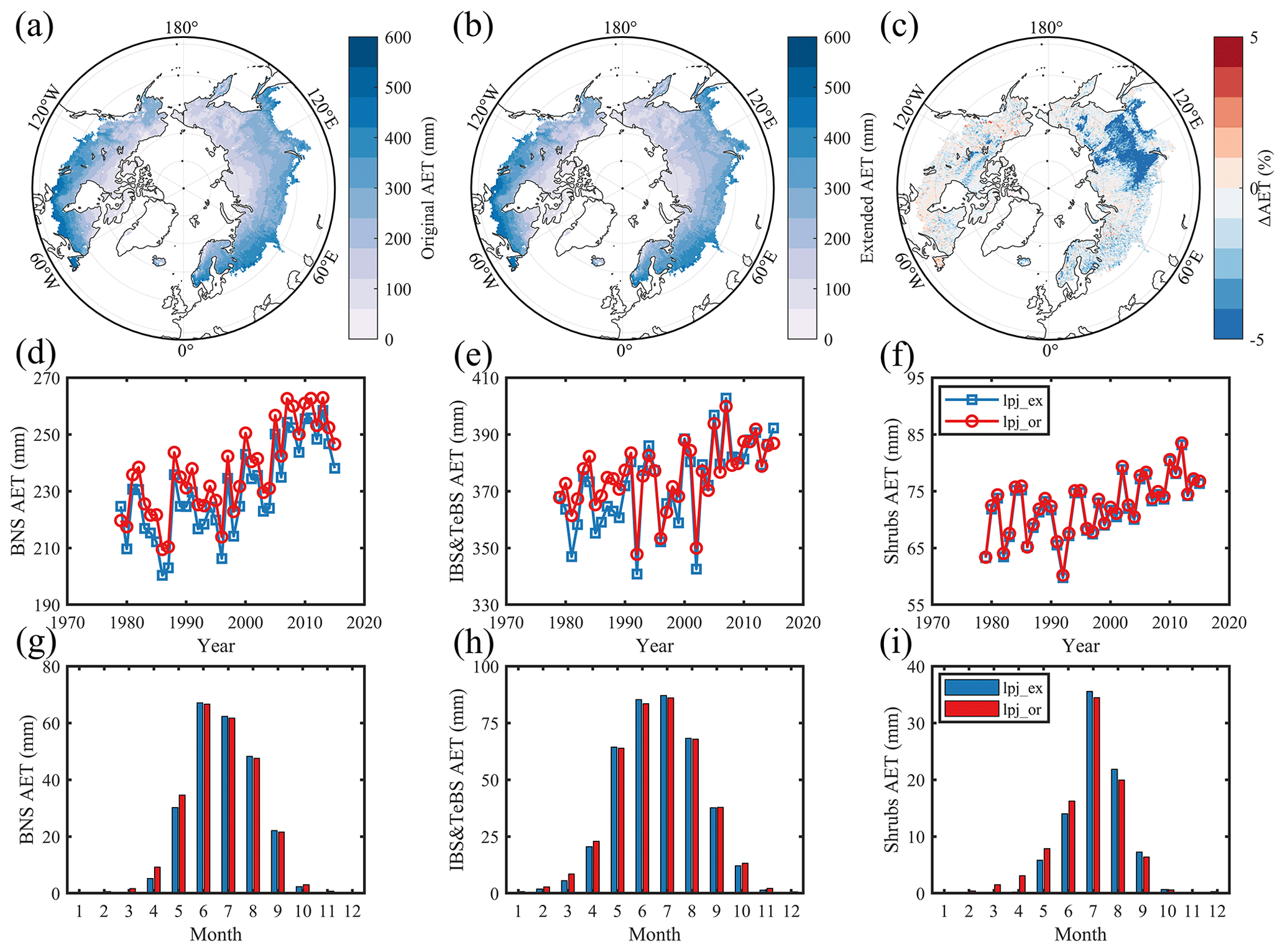
Figure 6 Comparison of actual evapotranspiration simulations between scenarios which used the original phenological module and the extended (DORMPHOT and DM) phenological module. (a) This scenario used the original phenological module. (b) This scenario used the extended phenological module. Panel (c) shows the difference between the two scenarios mentioned above; blue represents a larger simulation value for the LPJ-GUESS model using the original phenological module, and red represents a smaller simulation value. (d–f) Annual average AET for BNS and IBS–TeBS trees and Shrub PFTs from 1979 to 2015. (g–i) Multiyear mean monthly AET for BNS and IBS–TeBS trees and Shrub PFTs from 1979 to 2015.

4 Discussion

4.1 Remote sensing phenology facilitates mixed-pixel phenology modeling

Whether through dynamic global vegetation model simulation or satellite remote sensing extraction, a key issue in large-scale vegetation phenology research is the scale transformation of phenology data in mixed pixels. For phenological extraction based on satellite remote sensing, which is a top-down approach, the spring phenology extracted from the mixed pixel (without specific dominant vegetation types) gives the information about the dates when the earliest plant leaf out occurs in the pixel, while the autumn phenology is the last one to experience senescence (Chen et al., 2018; Reed et al., 1994; White et al., 2009; Fu et al., 2014). Furthermore, previous studies have also detected temporal lags between the phenology of NDVI, LAI, and GPP, especially in tropical regions where the saturation of optical vegetation indices, such as NDVI and LAI, can limit the extraction of phenology; SIF (solar-induced chlorophyll fluorescence) data could overcome this issue (Guan et al., 2015; Li et al., 2021; Hmimina et al., 2013). In addition, the greenness of understory phenology (low shrub or grass in forests) further complicates the detection of overstory signals (Ahl et al., 2006; Tremblay and Larocque, 2001). It is challenging to separate remote sensing signals into different components by filtering or decoupling methods. The more feasible method is to detect phenological changes with a few mixed species at a small spatial scale and conduct climate-controlled experiments (Wolkovich et al., 2012).

The DGVM-based phenological simulation is based on a bottom-up method, which is different from phenological extraction based on remote sensing. Many studies have investigated phenological algorithms based on remote sensing data and ignored the influence of mixed pixels (Keenan and Richardson, 2015; White et al., 1997), which lacks extensibility and robustness under changing circumstances, e.g., climate change. DGVMs simulate plant individuals' growth, development, and senescence in the grid cell, which represents different signals in the mixed pixels and finally synthesizes the vegetation signal of the whole grid cell (Sitch et al., 2003). In this study, based on top-down remote sensing phenology and parameter calibrations for several relatively pure pixels with a clear dominance of BNS and IBS–TeBS trees and Shrub PFTs, we integrated this newly calibrated phenology module at a PFT level into the LPJ-GUESS to reproduce the grid-cell-level vegetation phenology for the mixed pixels. The simulation of vegetation phenology for mixed pixels enables the capture of phenological variability arising from dynamic vegetation changes, as opposed to the predefined approach reliant on specific pixel vegetation types; this also partly explains why phenological algorithms based on predefined vegetation types are difficult to generalize spatially (Chen et al., 2018). By leveraging the advantages of wide-ranging remote sensing phenological monitoring and stable monitoring frequencies, analyzing the relationship between pixel constituents and vegetation signals, especially in cases where pixel constituents are relatively uniform, can enhance the accuracy of the phenological simulation for mixed pixels.

4.2 Influence of phenological shifts on ecosystem structure

Our results showed that the LPJ-GUESS model, which uses the original phenological module, estimated earlier SOS in regions dominated by BNS and IBS–TeBS trees and Shrub PFTs than it did when using the extended phenological module (Fig. 3). Earlier spring phenology, which is closely related to plant growth and development and has a strong influence on interspecific competition (Roberts et al., 2015; Rollinson and Kaye, 2012), also leads to a larger dominant area (Fig. S3). In the high-latitude regions, plants gain a competitive niche through the advancement of spring phenology if there is no damaged tissue and shoots that are induced by late frost and the weight of late snowfall (Augspurger, 2009; Bigler and Bugmann, 2018; Drepper et al., 2022; Liu et al., 2018b). This advancement is mediated by the early snowmelt synergistic changes in soil temperature and soil water content. It manifested in a wider window of high resource availability and low competition (Zheng et al., 2022). During this window period, plants can get more light, water, and nutrient resources and then carry out vegetative growth earlier. They can then finally increase the leaf area in spring. As the community develops, changes in the competitive relations at the species or functional group level in the spring will induce changes in community composition (Morisette et al., 2009; Forrest et al., 2010). In the context of climate change, differences in the phenological responses of different species may further affect the distribution of species, and the inaccuracy of future phenological dynamic simulations of different vegetation types in DGVMs will introduce great uncertainty to the estimation of future potential natural plant distribution (Dijkstra et al., 2011); this further impacts the GPP simulations, which are a key source of uncertainty for terrestrial carbon cycle simulations (Ahlström et al., 2015).

4.3 Further development of phenological algorithms

Although we have substantially improved the accuracy of LPJ-GUESS in simulating vegetation phenology by coupling calibrated spring (DORMPHT) and autumn (DM) phenological algorithms at PFT levels, we still see the discrepancy in the grass-dominated regions, and because of this, we did not employ the temperature and photoperiod phenological algorithm for the grassland phenology simulation because many studies indicate that grassland phenology is also regulated by precipitation (Fu et al., 2021). Furthermore, the current phenology algorithms only consider the synergistic effects of temperature and photoperiod but can be further linked to plant growth and physiology (Fu et al., 2020; Zohner et al., 2023). In different regions (under different external conditions), the driving mechanism and effective driving factors of the vegetation phenology process can be different. Temperature is an important factor regulating phenology in energy-limited regions, while water supply (precipitation, soil moisture, etc.) control cannot be ignored in water-limited regions (Prevéy et al., 2017; Fu et al., 2022). On the one hand, for further developing phenological modules in DGVMs, it is necessary to carry out mechanism research of phenology of different species through controlled experiments, to the end of improving the existing mechanism algorithm. On the other hand, it is necessary to introduce new methods, such as machine learning, for the accurate generalization of some complex key nonlinear processes (Fu et al., 2020; Dai et al., 2023). Through the above two aspects of work, a comprehensive phenological module can be provided in order to further improve the accuracy of DGVMs in simulating the phenological dynamics of different PFTs in different environments.

5 Conclusion

In this study, we parameterized and constructed spring (DORMPHOT) and autumn (DM) phenology algorithms for BNS and IBS–TeBS trees and Shrub PFTs based on the remote-sensing-extracted phenology data. These parameterized DORMPHOT and DM algorithms were further coupled into the LPJ-GUESS model, and the results showed that LPJ-GUESS, using the extended phenological module, substantially improved in the accuracy of spring and autumn phenology compared to the original phenological module. Furthermore, we found that the differences in phenological estimations can have non-negligible effects on carbon and water cycle processes by influencing plant annual growth dynamics and ecosystem structure functions. For the carbon cycle, the influence of phenological differences on BNS-dominated and Shrub-dominated regions was greater than that of IBS–TeBS-dominated regions, and there were differences in the seasonality of monthly GPP simulations with different PFTs. For the water cycle, the AET simulations become higher in spring and lower in summer, and only in the Shrub-dominated region does the AET simulation become lower in autumn when the original phenology module is used. We highlighted the importance of phenology estimation and its process interactions in DGVMs and proposed further developments in vegetation phenology modeling to improve the accuracy of DGVMs in simulating the phenological dynamics and terrestrial carbon and water cycles.