Tomofast-x 2.0: an open-source parallel code for inversion of potential field data with topography using wavelet compression

We present a major release of the Tomofast-x open-source gravity and magnetic inversion code that incorporates several functionalities enhancing its performance and applicability for both industrial and academic studies. The code has been re-designed with a focus on real-world mineral exploration scenarios, while offering flexibility for applications at regional scale or for crustal studies. This new version includes several major improvements: magnetisation vector inversion, inversion of multi-component magnetic data, wavelet compression, improved handling of topography with support for non-uniform grids, a new and efficient parallelisation scheme, a flexible parameter file, and optimised input–output operations. Extensive testing has been conducted on a large synthetic dataset and field data from a prospective area of the Eastern Goldfields (Western Australia) to explore new functionalities with a focus on inversion for magnetisation vectors and magnetic susceptibility, respectively. Results demonstrate the effectiveness of Tomofast-x 2.0 in real-world studies in terms of both the recovery of subsurface features and performances on shared and distributed memory machines. Overall, with its updated features, improved capabilities, and performances, the new version of Tomofast-x provides a free open-source, validated advanced and versatile tool for constrained gravity and magnetic inversion.

1 Introduction

In spite of the long-recognised ambiguities in the geological interpretation and inversion of gravity and magnetic datasets (Nettleton, 1942), these two methods remain popular approaches to understanding the continental subsurface. This is at least in part because, unlike theoretically more informative methods such as the array of seismic techniques, there are already widespread gravity and magnetic databases available for most continental areas. In addition, unlike geophysical methods such as gamma ray spectroscopy or synthetic aperture radar, there is significant 3D information content in the data.

Table 1 Some of the more popular open-source 3D gravity and magnetic inversion platforms.

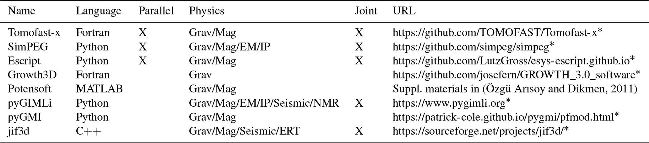
^* Last access: 11 March 2024.

One of the challenges faced by geophysical inversion platforms is to make them scalable, meaning that they not only meet the expectations of research geophysicists trialling new algorithms but can actually be applied to large-scale industrial and governmental applications. As part of their exploration programme mineral explorers will often undertake an unconstrained 3D inversion of the available magnetic or gravity data in order to better understand the 3D architecture and to generate prospects. As more data are acquired these unconstrained inversions may be re-run with geological constraints and new datasets. Similarly, government agencies also need to undertake 3D inversions at a relatively large scale in order to help their geological mapping teams understand the 3D architecture. While they may be less pressed by time constraints than explorers, they will typically be working with much larger datasets. Tools that can scale from prospect to regional scale are required.

There has been a long history of forward modelling (Jessell, 2001) and inversion of gravity and magnetic datasets (Pears et al., 2017). For much of the past 20 years the tools of choice for most explorers and government agencies have been the inversion codes developed by the Geophysical Inversion Facility (GIF) at The University of British Columbia (UBC) (Li and Oldenburg, 1996a, 1998). Over the past decade many explorers have switched from the GIF-based tools to the Seequent's Voxi product, the interface for which is built into the commercial Windows-based software tools they often use. Voxi is provided as a commercial cloud-based Software as a Service (SaS) running on clusters. There are several other less commonly used commercial programs for 3D potential field regularised inversion, each with unique specialisations (e.g. Geomodeller, VPmg and MGinv3D).

More recently, there has been an increasing focus on developing open-source solutions to solve the gravity and/or magnetic inversion problem, which provide access to inversion solutions to a wider audience (Table 1). When the inversion facility at UBC wound down, several of the researchers moved to make the algorithms open source and available in Python in the hope they would be adopted as a teaching and research tool. This project is known as SimPEG and now has a sizeable user group of academic, government, and industry users, particularly in North America (Cockett et al., 2015). The Python code has been built from scratch using many similar problem formulations to the original Fortran code used in the GIF packages. It uses public libraries (e.g. NumPy) for I/O and for the solver and leverages new advances in high-performance computing (dask and zarr libraries) to improve performance. It is, however, significantly slower than the older Fortran codes and does not offer a practical solution for typical, exploration-sized, datasets. Compression is only on file size, not matrix size, and therefore does not offer rapid solutions to many real exploration problems. To the best of our knowledge, among the open-source codes listed in Table 1, Tomofast-x is the only one that offers wavelet compression of the sensitivity matrix.

Each of these 3D platforms has strengths and weaknesses in terms of scalability, ease of installation, ease of generation of input meshes, reliance on commercial platforms, etc., even before we think of specific functionality and the additional constraints that can be added to the inversion to try and reduce the aforementioned ambiguity. This paper does not attempt to benchmark the different codes, interesting as that would be and much as that would be a worthy collaboration between the different research groups currently maintaining these codes. What has been missing from this mix is an open-source package able to scale to continental-sized problems while offering rapid answers at prospect scale. Tomofast-x is such a package.

When Tomofast-x was publicly released in 2021 it strongly reflected its research origins. Any exploration problem of reasonable size required a large cluster to solve in anything approaching real time, and for magnetic inversions observations had to be above the highest point in the model space. It only inverted in terms of susceptibility and density. Through a close collaboration between industry and academia it now offers equivalent performance and results to commercial codes. In addition, in addition to susceptibility and density it now also inverts in terms of magnetisation using either single-component total magnetic intensity (TMI) data or three-component magnetic data.

2 Description of code features

Tomofast-x inversion code is written in Fortran 2008 using classes, which allows flexibility in extending the code, such as adding new types of constraints, algorithms, and data I/O. It is fully parallelised using the MPI library, which provides both shared and distributed memory parallelism. The code has parallel unit tests covering important parts, which are implemented using “ftnunit” framework (Markus, 2012) extended by us to the parallel case to work with the MPI library.

Figure 1 Tomofast-x 2.0 inversion workflow. New components are highlighted in orange.

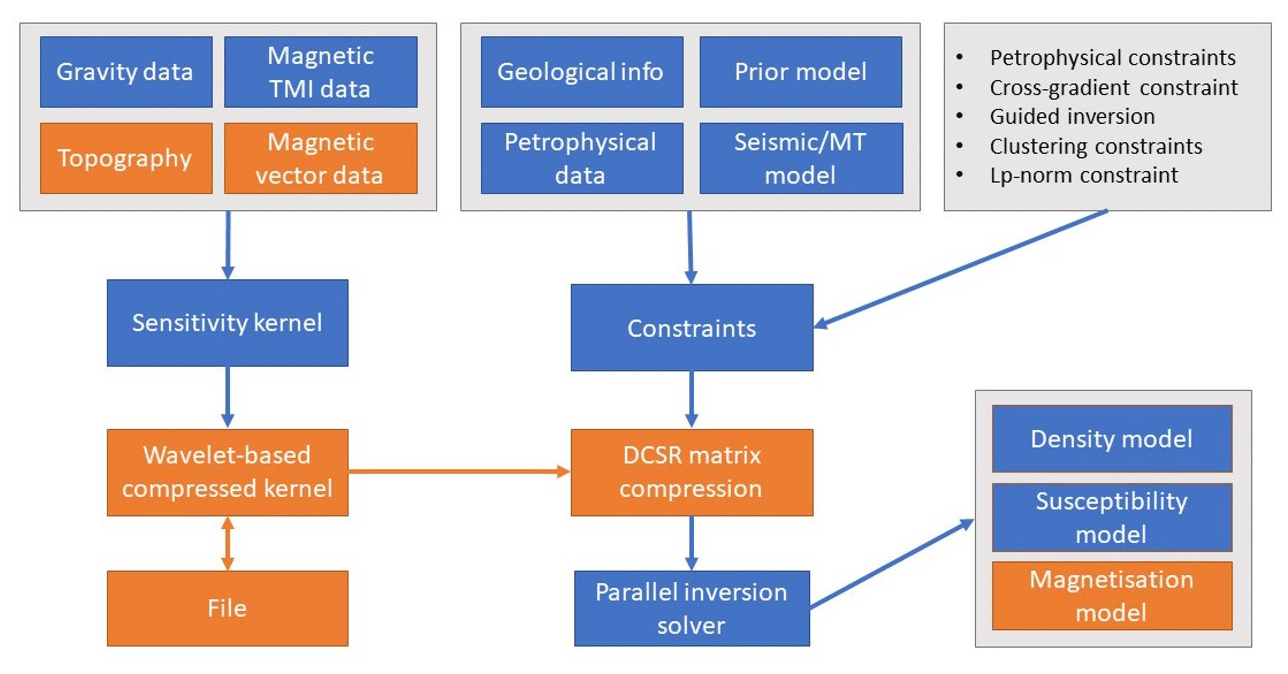
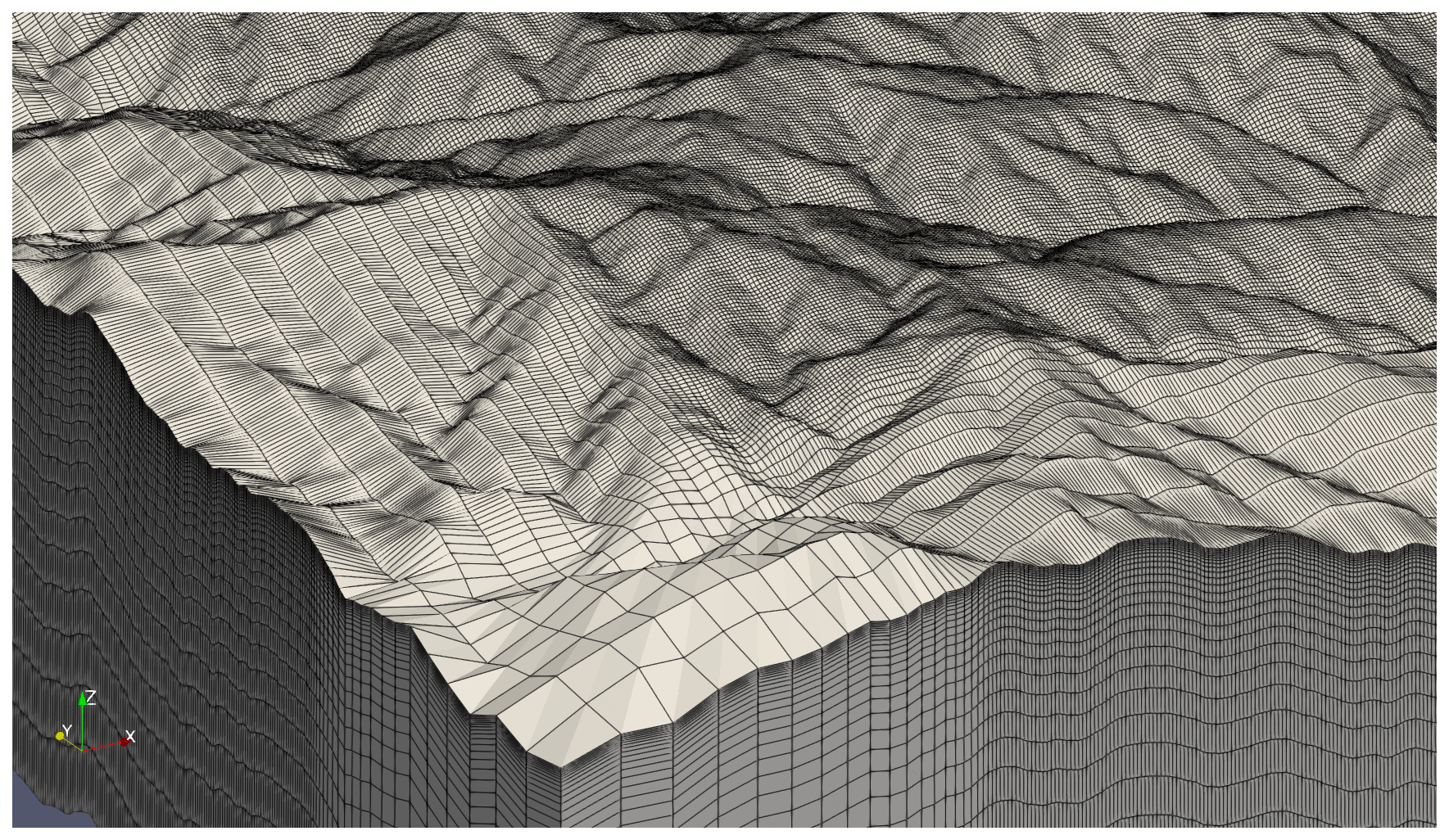
Figure 2 A non-uniform model grid with topography for the Synthetic400 model (for more details on this model, see Sect. 3.1).

The previous code version Tomofast-x 1.0 included geological and petrophysical constraints implemented, specifically clustering constraints (Giraud et al., 2019b), cross-gradient constraints (Martin et al., 2021), local gradient regularisation (Giraud et al., 2019a, 2020), Lp-norm constraints (Martin et al., 2018), and disjoint interval bound constraints (Ogarko et al., 2021; Giraud et al., 2023b), which were summarised in Giraud et al. (2021). Figure 1 shows a summary of the Tomofast-x 2.0 inversion workflow, and new components added to the version 2.0 are highlighted in orange. In this section we describe new code components added to Tomofast-x 2.0 code version and highlight their importance.

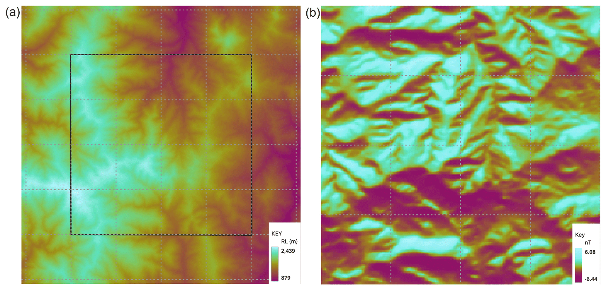
Figure 3 (a) Synthetic400 model topography of the whole model. (b) Forward magnetic response of the model's core from the topography alone. The outline of the core is shown in (a). The dashed lines are a 2500 m × 2500 m graticule.

2.1 Topography

The impact of topography on gravity data is well known. Less well understood is the effect of topography on magnetic data. However, as clearly demonstrated by Frankcombe (2020), it is important to include topography in magnetic modelling. In modern volcanic terrains where moderately magnetic andesitic basalt makes up a large proportion of the sub-crop and topography is often severe, the magnetic signal from topography alone can be tens to hundreds of nanoteslas. This may be greater than what might be a relatively subtle response from a deeply buried body. Failing to account for topography not only risks missing subtle targets, but it will also lead to erroneous interpretations if the magnetic data is interpreted or inverted on the assumption that the ground is flat.

There are several approaches used to include topography in the model, the most simple being to ensure that the model space is a rectangular prism extending into air above the highest point in the topography. A more advanced approach is to use a tetrahedral mesh to smoothly model the topography. Intermediate approaches and that used by this code are to drape a rectilinear mesh below the topography. This required that the topography is discretised into steps the size of the mesh cells but does not require that the air be included in the model. As each vertical pillar of cells in the model is independent, there is no need for each layer of cells to have a fixed top and bottom. This enables the topography to be discretised into locally thin layers without requiring that all points in the model at that elevation have the same fine discretisation. In areas of severe topography, draping the mesh below the topography and treating each vertical pillar of the mesh independently significantly reduces the size of the mesh, and thus the run time, relative to regular rectangular prism meshes. Figure 2 shows an example of a model grid with topography.

The forward magnetic problem in Tomofast-x 1.0 was calculated using Bhattacharyya's formulation (Bhattacharyya, 1964). It has the limitation that all data locations must be above the highest point of the model. Modern aeromagnetic data are acquired at heights of less than 40 m above ground. There are very few project areas which have less than 40 m difference in elevation across them, limiting the utility of Bhattacharyya's algorithm. In order to allow for arbitrary topography and readings below the Earth's surface, the forward magnetic problem was re-implemented using Sharma's formulation (Vallabh Sharma, 1966). Additionally, distance-based weighting of the sensitivity kernel, which is a generalised version of a simple depth weighting, was included (Li and Oldenburg, 1996b). Weighting by distance rather than depth allows for observations beside or even below points in the model.

2.2 Non-uniform model grid

The size of a regularised inversion is (N_data+1) × N_model, where N_data is the number of observations being modelled and N_model is the number of cells in the model mesh. When stored as 8 byte reals this leads to around 7.5 Gb being required for a 100 × 100 × 10 model block with a 100 × 100 array of observation points. Such a tiny model size would only be used for test work. For an ordinary exploration sized problem tens of petabytes might be required while for government-style regional work exabytes or zettabytes of storage would be needed. While large problems can be broken up into smaller panels and then re-joined (Goodwin and Lane, 2021), care needs to be taken to avoid edge artefacts, and the overall time to run the inversion is considerably longer because of the need to run coarse inversions followed by forward models to minimise these edge effects. In addition, large problems require more computational cycles placing an effective limit on the size of problems that can be handled. In order to reduce the size of the problem, the voxel size can be increased for voxels distant from the observations. In practice it has been found that increasing the size of model voxels in a horizontal sense away from the core area containing the data and in a vertical sense below the ground surface reduces the size of the model array by about 40 times without degrading from the inversion result.

Care needs to be taken not to change the voxel size too quickly, as rapid changes in the volume sensitivity will result in material being moved from a smaller, lower-sensitivity cell to its larger neighbour, introducing artificial stratification to the inversion model. A multiplier of around 1.15 with a hyperbolic tangent smoothing into the core of the inversion area has been found to work well. Figure 2 shows an example of such a non-uniform model grid.

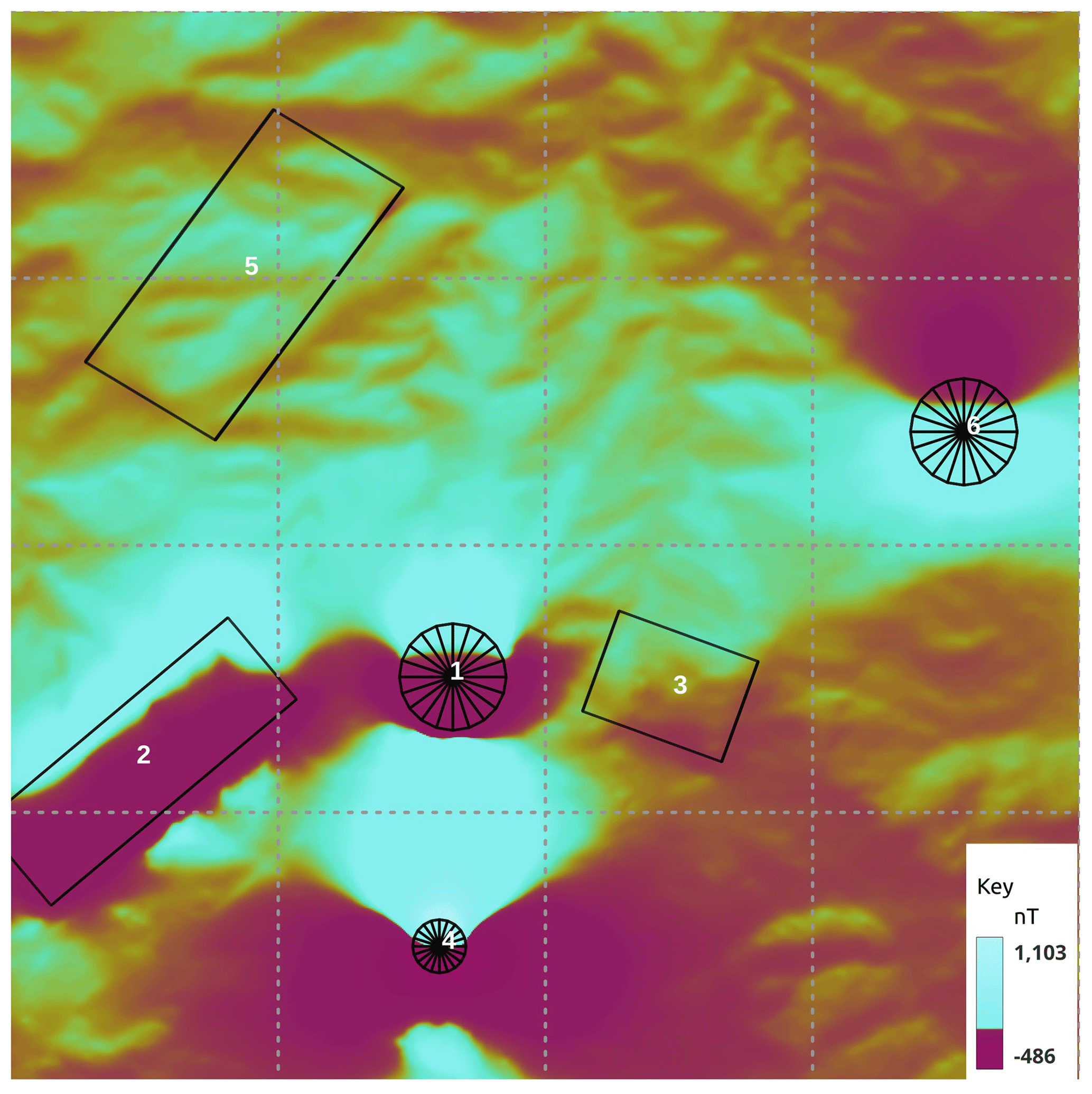
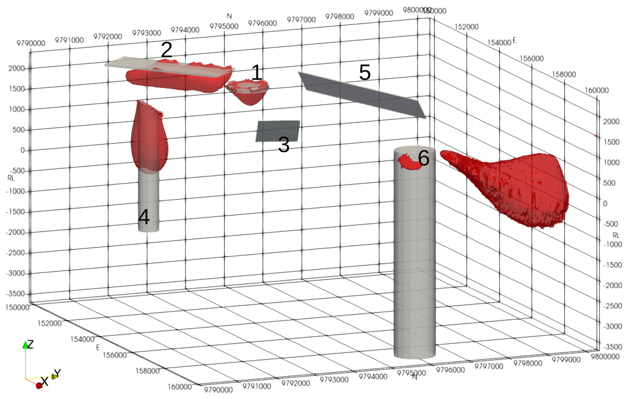
Figure 4 The Synthetic400 model's total magnetic response with magnetic body projections. The dashed lines are a 2500 m × 2500 m graticule.

2.3 Wavelet compression

Another tool to reduce the size of the inversion problem is to compress the matrices. Li and Oldenburg (2003) proposed using wavelet transforms to compress the sensitivity matrix by nulling all wavelet coefficients with amplitudes below a user-defined threshold. This approach can be used to reduce the size of the problem by up to 3 orders of magnitude without seriously impacting on the solution. Tomofast-x users have the option to choose between the commonly used wavelet, i.e. Harr and Daubechies D4 (Martin et al., 2013). The wavelet transform is implemented using multilevel lifting scheme, which reduces the number of arithmetic operations by nearly a factor of 2. The transform is performed in place, requiring only a constant memory overhead. The wavelet transform is applied to each row of the weighted sensitivity kernel independently, which are then compressed and stored using sparse matrix format (i.e. only non-zero values are stored). The resulting model perturbation vector after each inversion is transformed back from the wavelet domain using the inverse wavelet transform. As discussed in Sect. 2.1 the model grid is implemented by draping the mesh below topography. This allows the model grid to be defined as a 3D array of dimensions N_x × N_y × N_z for any topography without introducing additional “air” cells. The 3D wavelet transform can therefore be applied efficiently due to the coherency of the sensitivity values along the spatial dimensions. Unit tests were also added to verify that the wavelet transforms preserve a vector norm.

The non-compressed sensitivity kernel is a dense matrix of size N_data × N_model, with N_model = N_x × N_y × N_z. A user-selected compression rate R_c defines the fraction of sensitivity values to keep from the original kernel. Thus, the memory to store the compressed sensitivity kernel (using CSR format) nearly linearly scales with the compression rate and can be calculated as follows:

$$\begin{array}{}\text{(1)}& M_{\text{sensit}}=(\mathrm{4}+f)R_{\mathrm{c}}{N}_{\text{model}}{N}_{\text{data}}+\mathrm{8}{N}_{\text{data}}\mathrm{bytes},\end{array}$$

where f=4 for single-precision floating values and f=8 for double-precision floating values. Comparative tests showed that storing sensitivity values using single precision is sufficient and has no noticeable impact on inversion results, while it is important to use double-precision values during the sensitivity calculation and wavelet transformation. The first term corresponds to two arrays of the CSR format: column indexes (4 byte integers) and matrix values (floats). The second term in Eq. (1) corresponds to the array of indexes in the values array corresponding to each matrix row. It is stored using long integer type (8 bytes) to avoid integer overflow. An estimation of the total memory requirement is given in Appendix A.

An additional memory optimisation for the parallel matrix storage is discussed in Sect. 2.6, and examples of the inverted models using various compression rates are given in Sect. 3.3.

Figure 5 Inverted Synthetic400 susceptibility model. The contours are shown at k = 0.01 SI.

2.4 Magnetisation

Nearly all magnetic rocks will have a component of remanent magnetisation storing the magnetic field direction from the time of crystallisation of the magnetic mineral. The strength of this remanent field is often very weak and can be ignored; however, in a significant number of cases of interest to mineral explorers, the remanent field is strong enough to alter the shape of the observed field. Remanence can affect the host and the target. The existence of remanence is often evident from looking at the shape of the anomaly which should alert the interpreter to the potential for error. It may however be cryptic and if not allowed for, will result in a flawed interpretation.

In addition, all magnetic bodies are affected by self-demagnetisation. This is a property that produces a magnetic field within the body that is aligned to the shape of the body rather than to the Earth's field or any stored remanent direction. For bodies with susceptibilities less than 0.1 SI, the effects of self-demagnetisation are negligible; however, above this point the observed response can be distorted to such a degree that exploration programmes fail (Gidley, 1988). A solution to both problems is to invert on magnetisation rather than susceptibility (Elllis et al., 2012). The code was therefore extended to allow for magnetisation inversion.

It must be noted that magnetisation inversion needs three sensitivity kernels defined for each magnetic vector component (Liu et al., 2017). Thus, the computational and memory requirements grow by nearly a factor of 3. Therefore, using optimisations described previously (i.e. wavelet compression and non-uniform grid) becomes even more important for this type of inversion. Examples of magnetisation inversion are shown in Sect. 3.4.

2.5 Multiple data components

Historically only a single component of the magnetic field was measured. Initially the local declination or inclination were measured using optical dip meters; subsequently, the field strength in the vertical direction, Hz, was measured using a fluxgate. Fluxgates were replaced by proton precession and then optically pumped magnetometers that measured the field strength in the direction of the Earth's field, i.e. the total magnetic intensity (TMI). However, fluxgates can be used to also measure the horizontal components, as is routinely done within magnetic downhole survey tools. SQUID magnetometers are now being developed which will enable a tensor measurement. Multi-component data provide a more diagnostic dataset with regard to the body location, particularly when remanence is involved. It is therefore useful to be able to model and invert data acquired in any direction and from any location.

Inversion of three magnetic data components was included in the code. As with magnetisation inversion discussed in previous section, this also increases the computation and memory requirements. Specifically, when three data components are used for magnetisation inversion, the number of the sensitivity kernels grows to nine. Thus, these inversions strongly benefit from wavelet compression and non-uniform grid optimisations. These modifications allow for inversion of three-component downhole magnetic data, which typically improves drill targeting compared to single-component or multi-component above-surface datasets. This improvement is particularly noticeable when magnetic remanence is present.

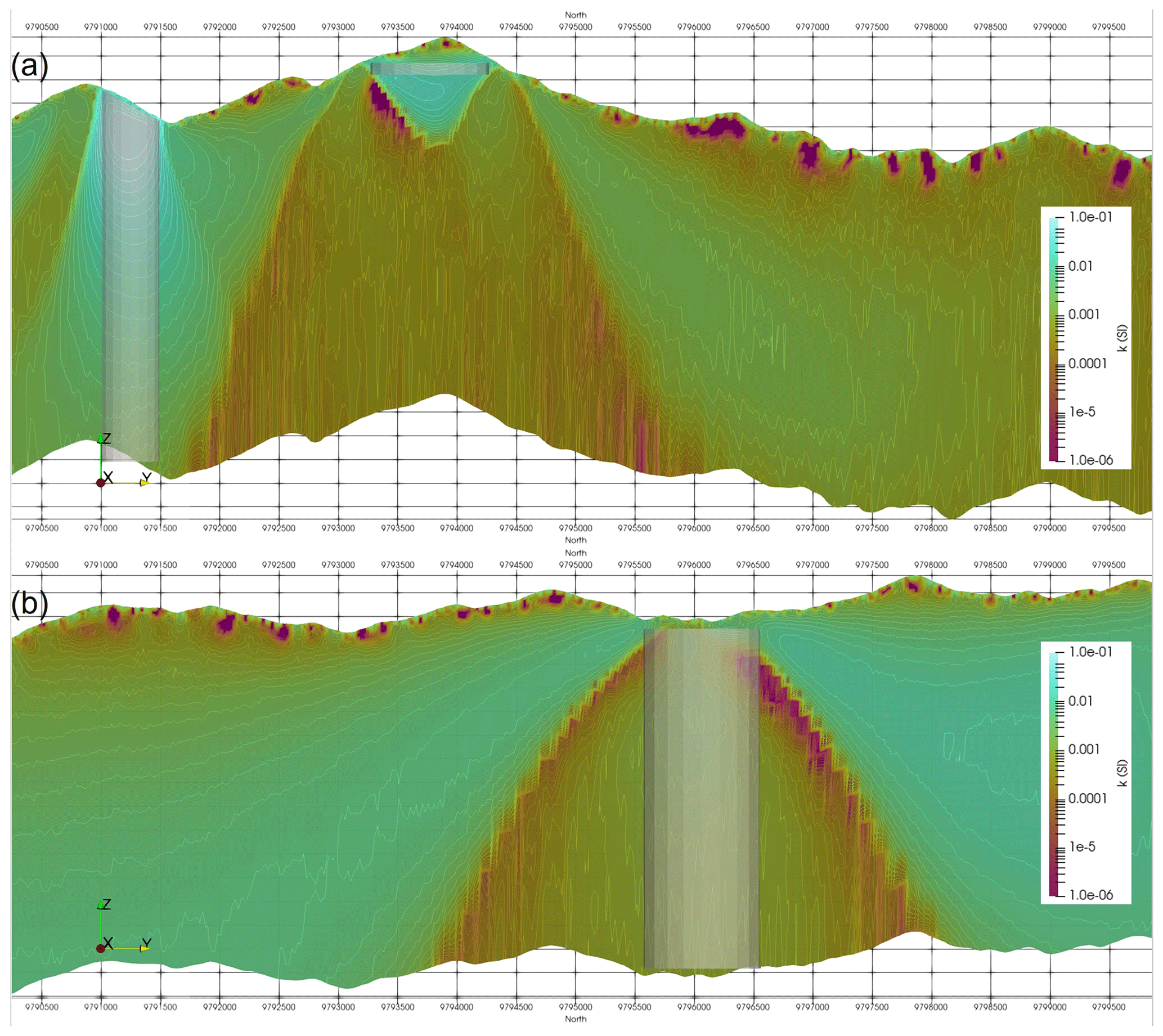
Figure 6 Vertical sections of the inverted Synthetic400 model through (a) a high-susceptibility cylinder and disc and (b) a low-susceptibility cylinder.

2.6 Efficient parallelisation scheme

The parallelisation of the inversion problem can be approached in several ways: by partitioning the model or partitioning the data. These two approaches correspond to splitting the least-squares system matrix by column (model) or by row (data). As both approaches have their advantages, an efficient parallelisation scheme that combines the two approaches was designed. The parallelisation scheme is comprised of the following elements.

The forward problem is parallelised by data. This avoids the need to parallelise the wavelet compression, as the full row of the sensitivity kernel (corresponding to the whole model) is available at each processor. This in turn allows for saving costs in terms of the MPI communication required to parallelise the wavelet compression. This can be significant as the wavelet transform calculations are non-local and span over the whole model space.

The inverse problem is parallelised by model. In the compressed sparse row (CSR) matrix storage the model vector is accessed in the inner loop in both matrix vector and transposed matrix vector products. This limits the performance due to memory traffic (Sect. 4.3.2 in Barrett et al., 1994). In order to minimise the memory traffic in these operations it is better to partition the model vector. Both versions with the inversion problem parallelised by data and by model were implemented and compared, confirming that parallelising by model is faster and leads to better scalability. This was also confirmed by profiling the code using Intel VTune Microarchitecture Exploration tool, which showed an increase in L3 cache misses relative to partitioning by model, resulting in an overall slowdown of the code. Machines with larger L3 caches performed better than those with smaller caches even though they had older-generation CPUs.

Load balancing is performed in the following way. When wavelet compression is applied to the sensitivity kernel, the distribution of the non-zero values is not uniform. When the model partitioning is performed using equal size chunks, the number of non-zero kernel elements can vary by a factor of 100 on different processors. This leads to non-efficient usage of CPU resources and slows down the calculations. To mitigate this, load balancing was implemented by partitioning the matrix columns into non-equal chunks such that the total number of non-zeros is nearly the same on each CPU.

Doubly compressed matrix storage is performed in the following way. In the CSR matrix storage format, the outer loop in the matrix vector and transposed matrix vector products iterates over the matrix rows. When parallelising the inversion by model (i.e. parallelising the inner loop), the outer loop spans over all matrix rows N_rows. This limits the parallelism, defined as the maximum possible speedup on any number of processors, to at most O(nnz$/N_{\mathrm{rows}}$) (Buluç et al., 2009), where nnz is the total number of non-zero values. The typical number of least-squares matrix rows in inversions is N_rows = N_data + N_c N_model, where the N_data-rows corresponds to the sensitivity kernel and N_model-rows corresponds to the N_c constraint terms (such as model damping term). The typical N_model value is much greater than the N_data, and thus adding constraints significantly limits the scalability. Note that the rows corresponding to constraint terms are usually extremely sparse, for example one non-zero element per row in the model damping term (i.e. a diagonal matrix). Thus, in the parallel runs there will be many empty rows in the local matrices, meaning that the redundant information will be stored. Therefore, the double compressed sparse row (DCSR) format, which improves the compression efficiency by storing only non-empty rows, was implemented (Buluc and Gilbert, 2008). The DCSR format adds one additional array to the CSR format, which stores the indexes of non-empty rows. This improves the scalability and reduces memory traffic. Additionally, this reduces the memory requirements for storing the matrix on several CPUs.

Efficient memory allocation is performed in the following way.In the LSQR inversion solver, the parallel bidiagonalisation operations (consisting of matrix vector and transposed matrix vector products) were re-implemented to overwrite the existing vectors, thus avoiding memory allocation for the intermediate products (for details, see Sect. 7.7 in Paige and Saunders, 1982). The corresponding parallelism was implemented using the same input and output buffer of the collective communication routine MPI_Allreduce via MPI_IN_PLACE.

In Sect. 3.5 the proposed parallelisation scheme is applied to several representative models, and the resulting parallelisation efficiency is also discussed.

Figure 7 Field TMI data for the Callisto model.

2.7 Sensitivity kernel import and export

The ability to import and export the sensitivity kernel has been implemented. The compressed sensitivity kernel is stored as a binary file, which allows for previously computed sensitivity kernels to be reused. This saves computational time (up to ∼ 95 %) when exploring the effect of different types of constraints and different hyperparameter values (i.e. when varying weights in the cost function), as well as different starting and prior models. The sensitivity kernel can also be reused when a different background field needs to be subtracted from the data, as the kernel values depend only on the model grid and data locations. Additionally, the calculated kernel can be imported into other codes to perform sensitivity analysis, null-space navigation, or level set inversions (Giraud et al., 2023a). Finally, it is possible to import the external kernel corresponding to a different geophysics or another optimisation problem (e.g. geological modelling) and use the Tomofast-x as a high-performance parallel inversion (or optimisation) solver. External to Tomofast-x, a Python script to import and export the sensitivity kernel from and to Python has also been implemented, and it is available at https://github.com/TOMOFAST/Tomofast-tools (last access: 11 March 2024).

Table 2 Model dimensions. In brackets the dimensions of horizontal padding are specified. Length values are given in metres.

Table 3 Description of the Synthetic400 model bodies.

3 Inversion examples

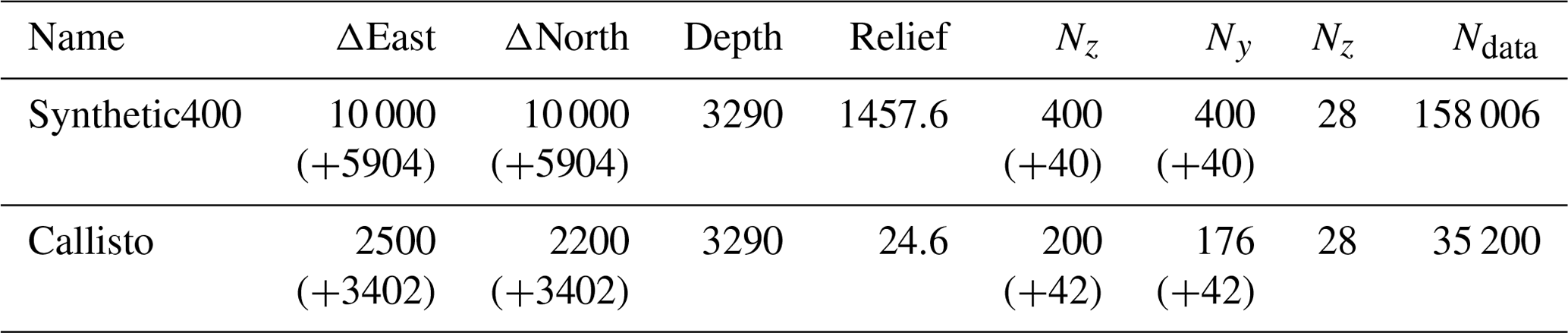
The datasets and models used for the inversion and the results of those inversions will now be discussed. Different compression rates were tested, and parallel performance was benchmarked. The Table 2 shows the physical model dimensions and corresponding model grid size and number of data for the test models, which are then described in detail below.

In all susceptibility inversions a positivity constraint was applied to reduce the model non-uniqueness (Li and Oldenburg, 1996a). The positivity constraint was added via the alternating direction method of multipliers (ADMM)-bound constraints (Ogarko et al., 2021). The number of major inversion iterations used was N_iter = 30 for Callisto model and N_iter = 50 for Synthetic400 model. The number of minor iterations (in the LSQR inversion solver) used was 100 in all tests.

3.1 Synthetic400 model

While it is important to use real datasets in testing inversion codes it is also important to use datasets where the answer is known. In real exploration datasets the true answer is never known, at least not throughout the model space. A drill hole here or there may constrain the depth to a particular magnetic body, and susceptibility measurements on core or chips or from in-hole tools may constrain the likely range of susceptibilities for that body. In general, however, the properties of the vast majority of the model space is unknown. Synthetic models are therefore required in order to calibrate the inversion algorithm and understand its target resolution. Although synthetic models can never achieve the level of complexity that a real dataset contains, this paper attempts to make the model as realistic as possible.

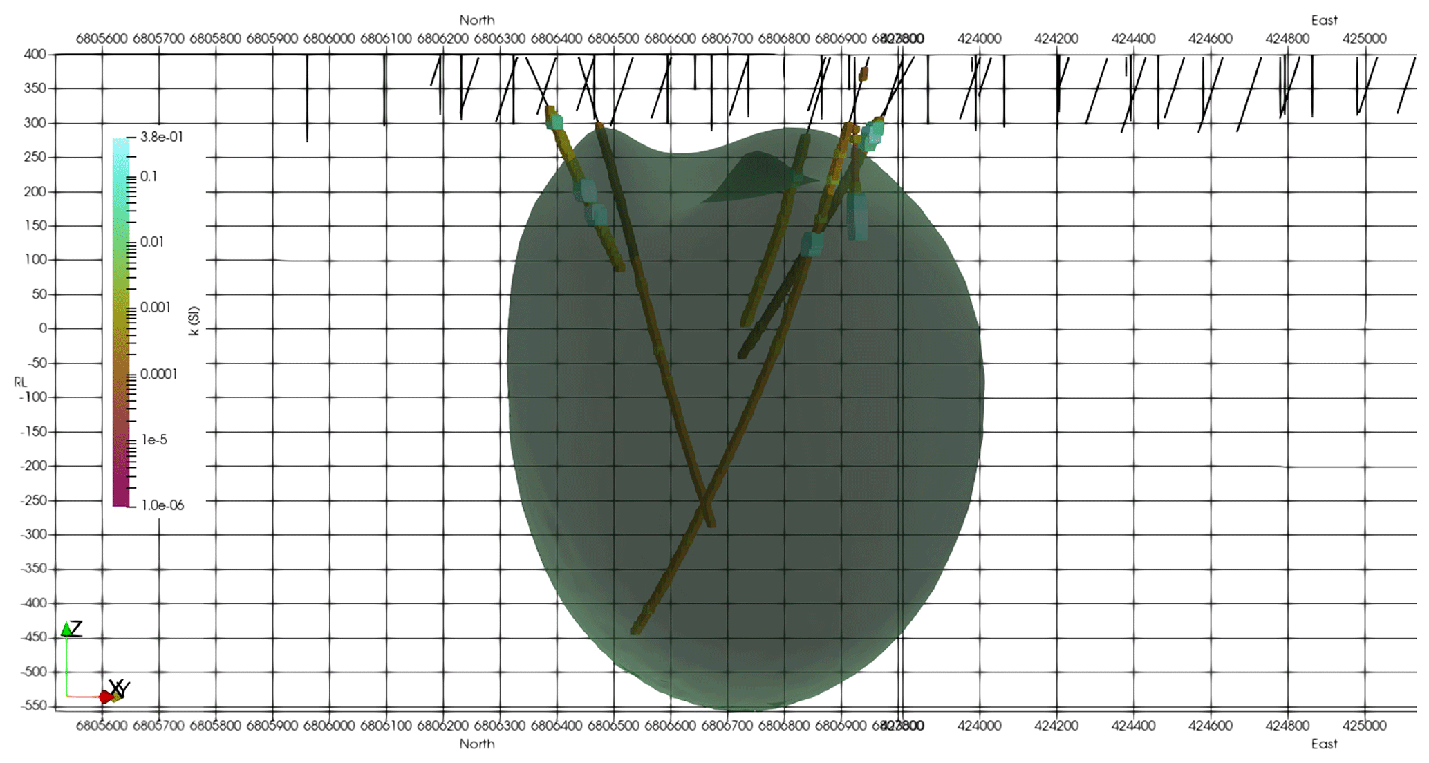
Figure 8 The inverted Callisto model with drill holes coloured and scaled by susceptibility. The model contour is shown for susceptibility k = 0.0126 SI.

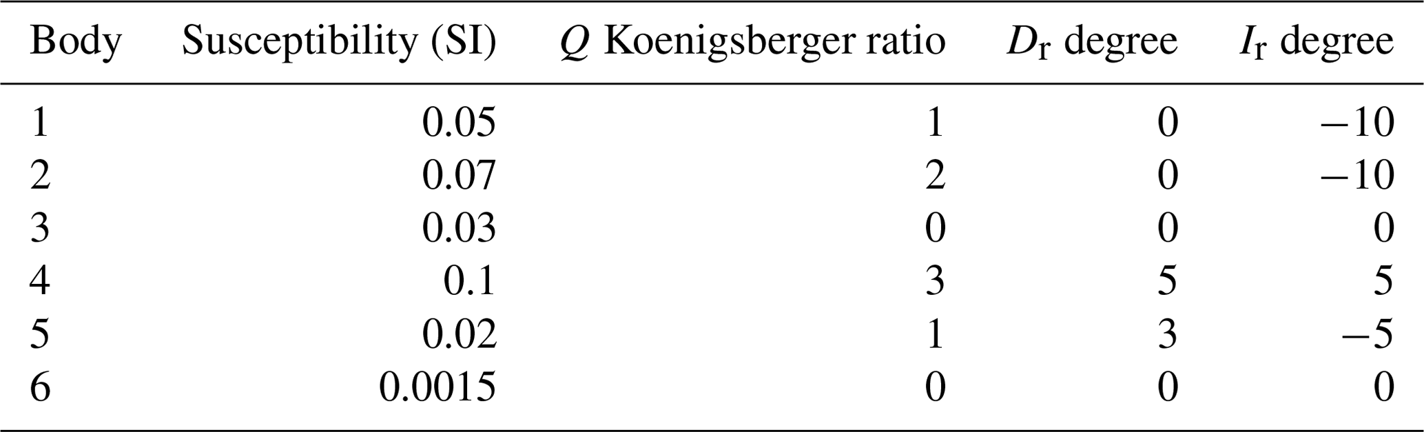
Table 4 Parameters used in the Synthetic400 model for magnetisation tests.

Topography, extracted from a 12.5 × 12.5 m ALOS DEM, for an active exploration prospect in Indonesia was used as the base layer, and the ground was ascribed a homogeneous susceptibility of 0.01 SI, which would be at the lower end of expected susceptibilities for this area. The elevation has a range of 1400 m over the 10 km × 10 km extent of the central core of the model space, increasing to 1600 m if one includes the horizontal padding. The magnetic response for a simulated survey flown with a perfect 60 m drape height over this topography was modelled using Tomofast-x, and the results are shown in Fig. 3 along with the topography that produced it. The field range shown in the key has been clipped to flatten the outer 2 % of the actual range, which was closer to 12 nT. As shown in Frankcombe (2020), typical topographically induced variations in these areas are an order of magnitude higher than this, implying a ground susceptibility closer to 0.1 SI. However, as we are looking at susceptibility contrasts, the use of a low background value in the synthetic model does not detract from its results. A parametric potential field modelling package (Potent – https://geoss.com.au/potent.html, last access: 11 March 2024) was then used to compute the magnetic response of several geologically plausible bodies buried in this topography. In order to provide a challenge for the inversion algorithm, the bodies were placed where their magnetic response might best be masked by topography. Potent uses line and surface integrals to model the response of bodies. Modelling the response of the host is only practical in 2D. Topography was used to control the sensor position, which was defined as a constant drape above topography. The susceptibility of the half-space is only used by the parametric modelling to compute a contrast to use when computing the response of the model body. The computed response therefore becomes the response from bodies in air. The susceptibility of bodies is their contrast relative to the host, which may be negative. These responses were then added to the computed response of the topography alone from Tomofast-x to generate a synthetic dataset. The Potent program was used in preference to a generalised voxel-based program because the regularisation of the mesh would have required very small voxels in order to accurately reflect the desired shape and thickness of the bodies. We have used a parametric model to better test the algorithm by approximating real-world structures that are hard to describe with a mesh of rectangular prisms.

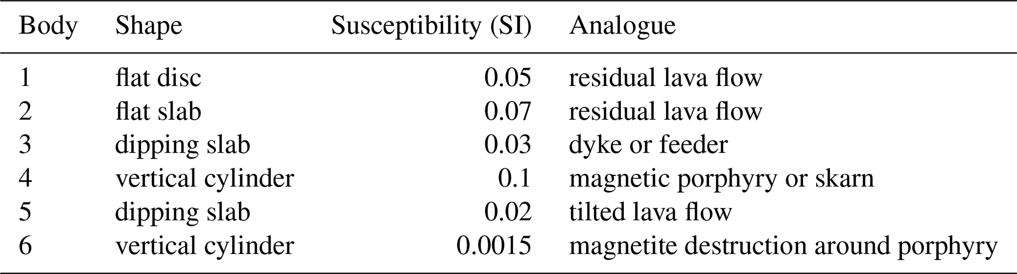
It is worthwhile saying a few words about the geological relevance of the synthetic model. In modern volcanic environments in the western Pacific and elsewhere, the underlying geology often consists of a series of volcanic flows. These range from relatively nonmagnetic crystal tuffs through to andesitic basalt and local lahar debris flows. Where the lahar carries andesite boulders it can become very magnetic and very heterogeneous. The layered package of volcanics may be interspersed with sediments deposited during periods of quiescence. These sediments are generally mudstones or limestones, but in deeper-water environments they may include greywackes. Typically, the package is only lightly tilted, meaning that dips are relatively flat. For the area to become of interest to explorers, an intrusion of some sort is required. These are typically pipe-like bodies and may have a positive susceptibility contrast with the host in the case of skarns and potassically altered porphyry-style mineralisation or, in the case of epithermal mineralisation or for the alteration halo around a porphyry system, a negative contrast through magnetite destruction. These elements have been incorporated into the synthetic model and are labelled in Fig. 4. Body 1 is a 100 m thick magnetic disc reflecting a more magnetic basalt flow that has been eroded away, except at the peak near the centre of the model space. Body 2 is a large, flat, 50 m thick, magnetic sheet similarly reflecting an erosional residual from broader magnetic lava flow. Body 3 is a 10 m thick dipping slab reflecting either a magnetically mineralised fault or a dyke-like feeder to the lava flows. Body 4 is a pipe-like magnetic body with a radius of 250 m and a relatively high susceptibility, reflecting a strongly potassically altered porphyry intrusion or skarn around a finger porphyry. Body 5 is a 20 m thick dipping sheet, reflecting a tilted magnetic lava flow. Body 6 is a 500 m radius pipe with a susceptibility lower than the host. This reflects a zone of magnetite destruction around and above a porphyry system. The bodies are described in Table 3.

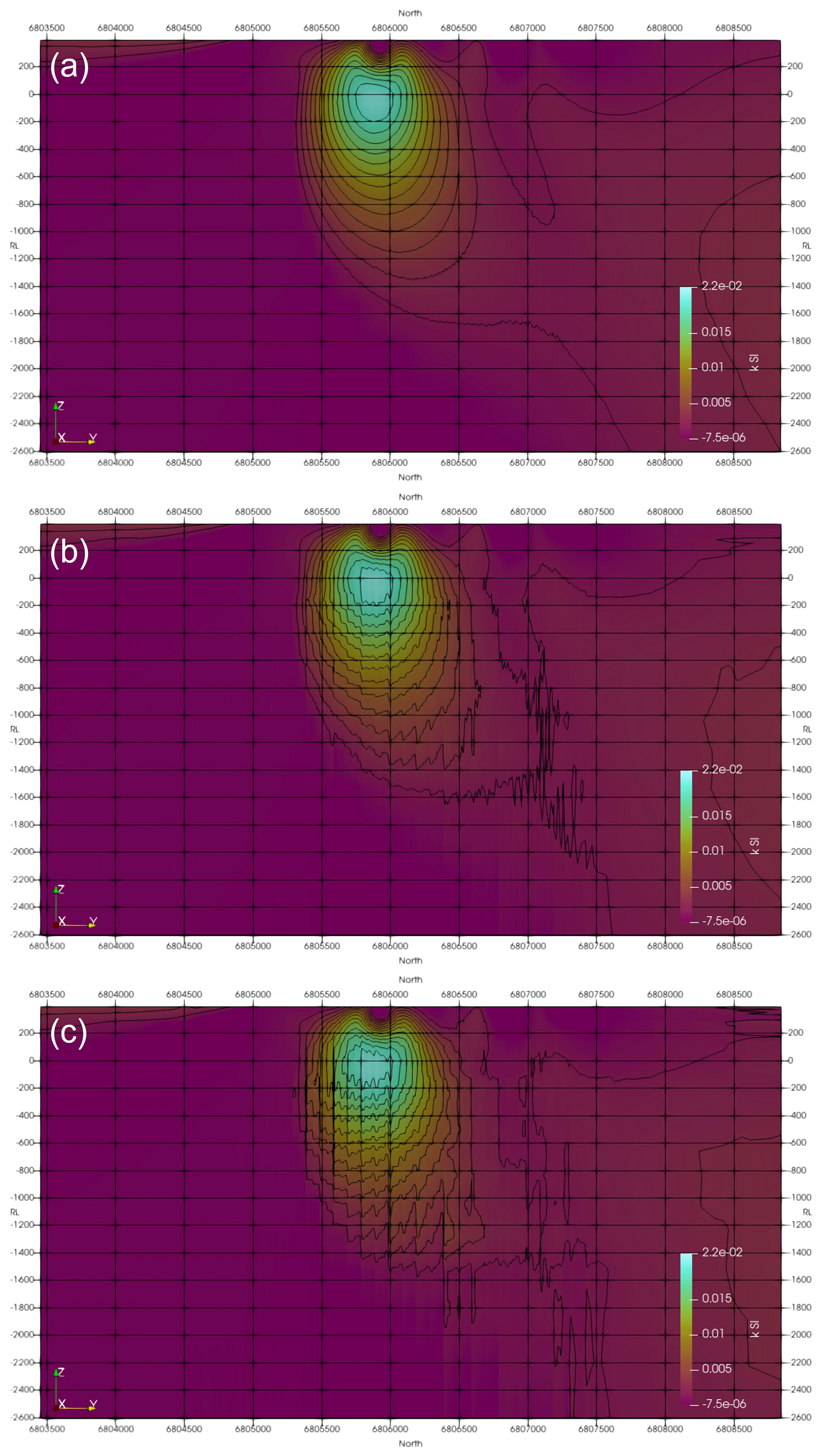
Figure 9 Inversion results for the Callisto model using different compression rates: (a) R_c = 5 %, (b) R_c = 1 %, and (c) R_c = 0.5 %.

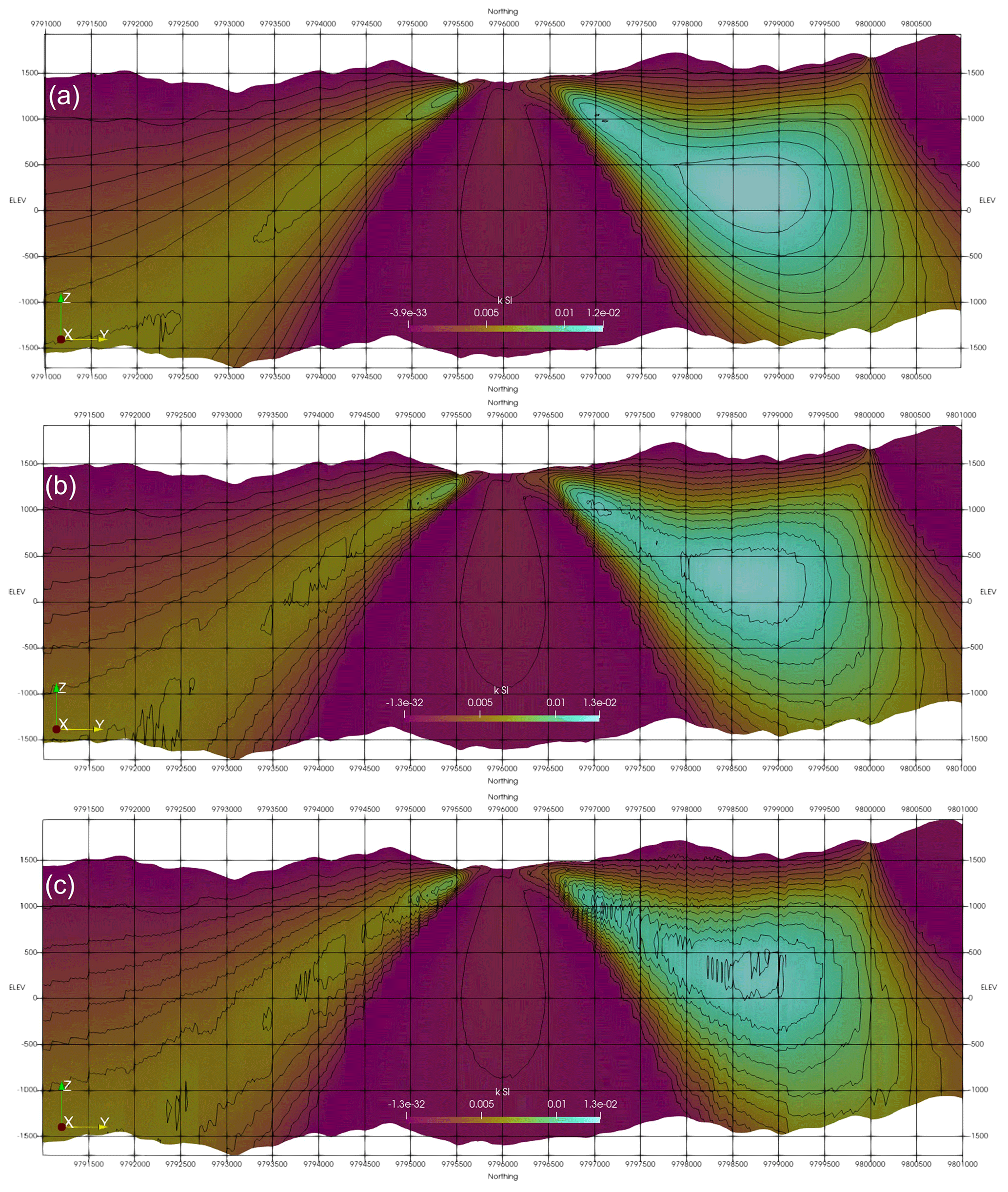
Figure 10 Inversion results for the Synthetic400 model using different compression rates: (a) R_c = 5 %, (b) R_c = 1 %, and (c) R_c = 0.5 %.

The synthetic data had various levels of noise added to it prior to inversion. Noise was added on the basis of a rescaled percentage of the observed value. Noise levels ranging from 1 % up to 10 % of the computed synthetic response were rescaled by a random number between −0.5 and +0.5. Where the amplitude of the rescaled noise fell below a noise floor, the noise floor multiplied by the sign of the rescaled noise replaced it. Noise floors of 1 and 5 nT were employed. That noise was then added to the computed synthetic response.

As this synthetic model contained no remanence, a susceptibility inversion was undertaken. A mesh with a central 400 × 400 voxel core of 25 m × 25 m voxels with a first layer thickness of 10 m was created. This was padded on each side with 20 cells increasing in size away from the core to add around 3500 m to each edge of the horizontal extent of the core, and 28 cells were used vertically to take the mesh down around 3200 m below the ground surface. In total the mesh was 440 × 440 × 28 cells (N_model = 5 420 800), and there were magnetic observations above the centre of each surface cell in the central core (N_data = 160 000). This would be considered a small- to moderate-sized exploration problem.

Regardless of the noise level, the inversion does recover the shape and depth to the top of the three most magnetic bodies (Fig. 5). The inversion favours the top of the vertical cylinder but focuses higher susceptibilities right to the bottom of the model as shown in Fig. 6a. It also places magnetic material beside the low-susceptibility body to compensate for what the inversion perceives as a negative susceptibility (Fig. 6b). This is a common artefact in unconstrained susceptibility inversions. For the thin slabs the inversion has overestimated the depth to the bottom of the body. This is also a common artefact and is driven by the smoothness of the L2 norm used to compute convergence.

The bowl-shaped overestimate of the thickness of body 1 has been compensated for by a “cape” of low susceptibility draped around the body. The noise added to the data is flowing through to the model as variations at the surface. Although the two thin dipping slabs with small susceptibility contrasts coincide with gradients in the model values, there is not enough contrast to be able to resolve these with any confidence. The bodies have susceptibility contrasts of 0.01 and 0.02 SI and are only 10 and 20 m thick, respectively. At the depth of the thin plates the model voxels are significantly thicker than the plates, and this means that not being able to resolve them is not particularly surprising.

The eastern body with a negative susceptibility contrast is poorly imaged, but as noted above this is typical for unconstrained susceptibility inversions. The inversion sees the body as having a negative susceptibility, but the positivity constraints will not allow this, meaning that magnetic material is artificially stacked around it to produce the response we see in Fig. 6b.

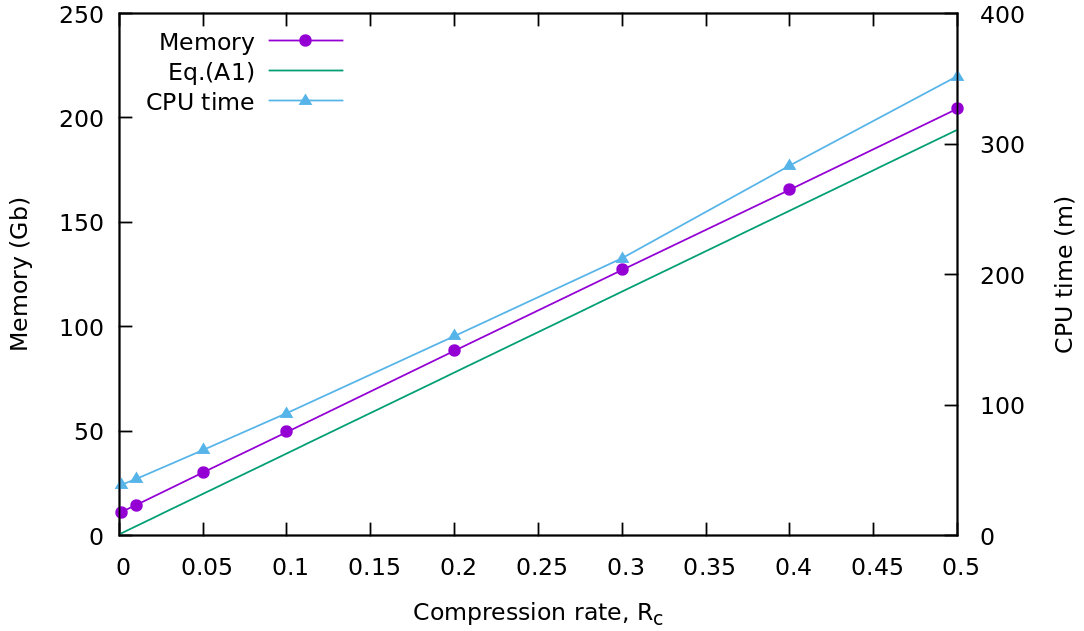
Figure 11 Memory usage and CPU time for different compression rates for the Callisto model using N_cpu = 40.

3.2 Callisto model

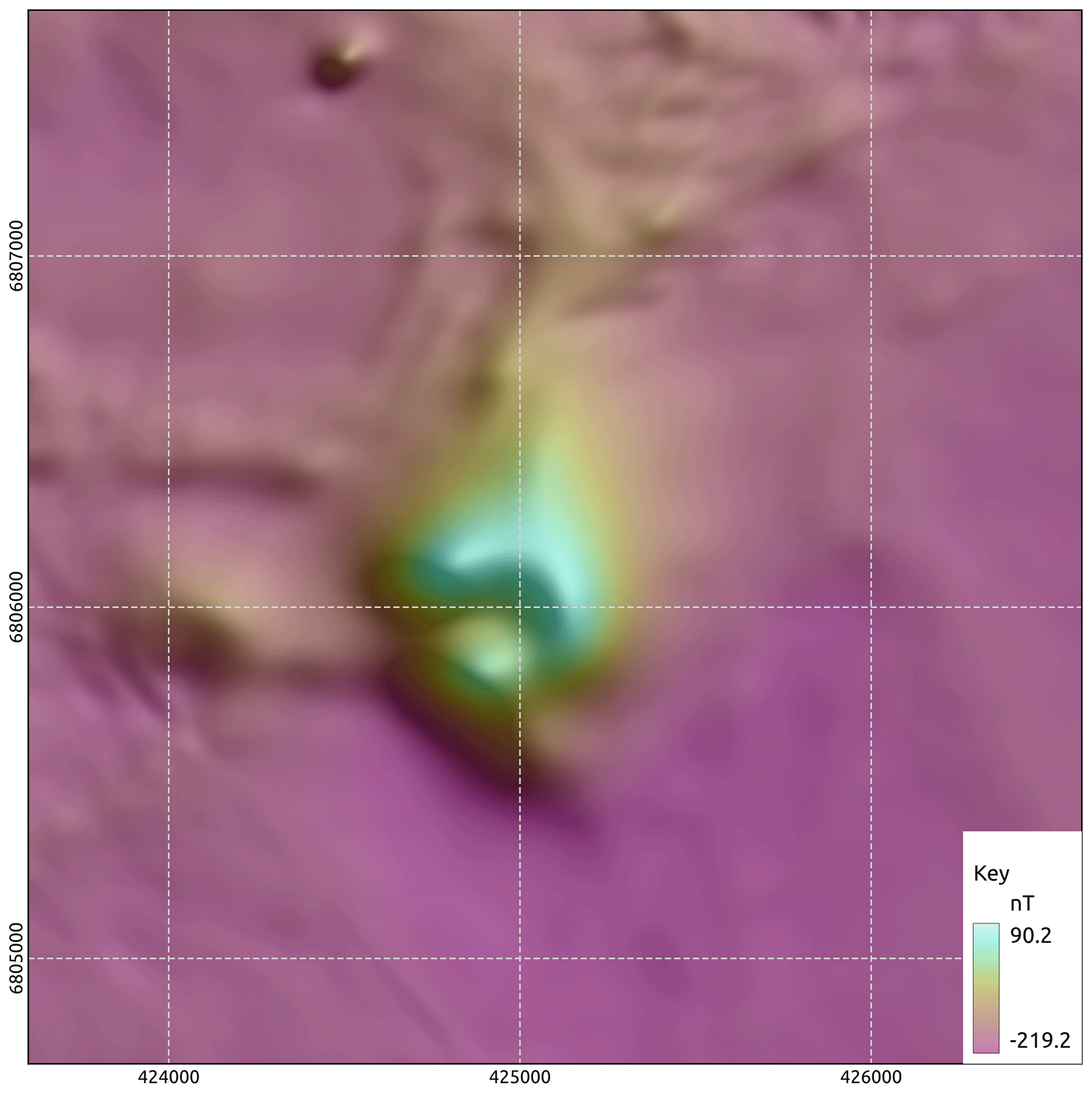
The Callisto anomaly is a discrete magnetic anomaly on the edge of Lake Carey in the Eastern Goldfields of Western Australia. Superficially it has many similarities with the neighbouring Wallaby and Jupiter magnetic anomalies, which are both magnetically mineralised syenite intrusions carrying significant quantities of gold (Wallaby > 7 MOz, Jupiter > 0.5 MOz). The area was flown in 1998 by its then owners, Homestake Gold of Australia, using 50 m line spacing and 40 m terrain clearance. The survey data are available from the Western Australian Department of Mines (https://geodownloads.dmp.wa.gov.au/downloads/geophysics/60251.zip, last access: 11 March 2024). The magnetic response of Wallaby has been studied in detail (Coggon, 2003; Banaszczyk et al., 2015), and although good fits to the observed data were obtained from modelling dipping cylinders, these models deviated from the geological model. Using susceptibility data from many drill holes, Coggon (2003) showed that the response could be modelled using a hollow pipe that reflected the geological model of a near-vertical zone of multiple syenite intrusions that had undergone a strong magnetite enrichment event followed by a strong magnetite destruction event associated with the gold mineralisation. This had created a residual annulus of high susceptibility around the altered gold-rich core. Figure 7 shows an image of the total magnetic intensity for Callisto that suggests that it too may be a hollow pipe-like body. It is thus a compelling exploration target.

Figure 8 shows the inverted model with drill holes coloured and scaled by susceptibility that has been measured on core using a handheld meter. There is a good match between increases in measured susceptibility and the edge of the magnetic model but a poor match inside of the inverted body, reinforcing the suggestion that the magnetite distribution has a hollow pipe-like shape. Although the shallow parts of the inverted model show fingers around a central low-susceptibility core, the smoothness in the objective function and a lack of constraining data causes the inversion to fill the pipe at depth. The same shape was recovered from an inversion of these data using the UBC MagInv3D package.

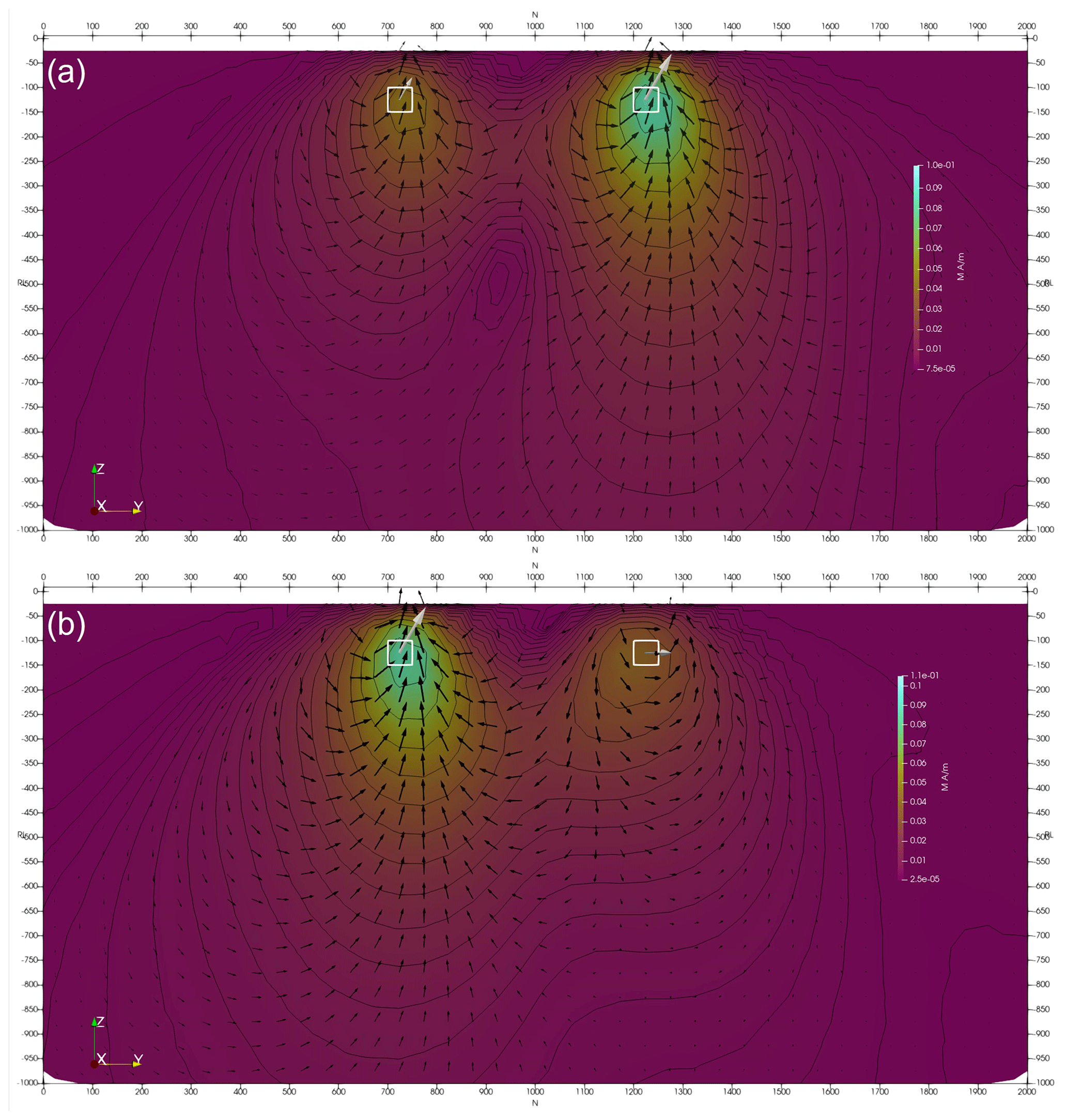
Figure 12 Inverted two-body magnetisation model where (a) both bodies are induced and (b) both bodies are remanent. The true model is shown with white vectors, and inverted model is shown with black vectors. The true and inverted models are not scaled the same, and they are both shown for the purpose of gauging fit to direction only. Images have a linear colour stretch, contours are drawn at logarithmic spacing, and vectors are scaled with the log of magnitude.

3.3 Different compression rates

To test the effect of differing compression rates, rates of R_c = 5 %, 1 %, and 0.5 %, corresponding to a reduction of the sensitivity kernel storage by factors of 20, 100, and 200, respectively, were applied. Figures 9 and 10 show a representative section through the inverted models. The effect of increasing degree of compression (i.e. decreasing compression rate) can be seen in the model contours. The weak compression, with R_c = 5 %, has nearly no influence on the structure of the resulting model. Stronger compressions, with R_c = 1 % and 0.5 %, result in noise in the contours, while the main model structures remain at the same location with the same shape and model values. As can be seen, the larger Synthetic400 model is less affected by compression than a smaller Callisto model. Generally, the larger the model, the greater the compression that can be used without significantly degenerating the model structure. This is due to the usage of multilevel wavelets, where larger models allow more levels to be used. For example, for the large model with dimensions of N_x = 812, N_y = 848, and N_z = 26, a compressed rate of R_c = 0.0086 was successfully used. The optimum compression rate can be either obtained experimentally or calculated from the available memory using Appendix A.

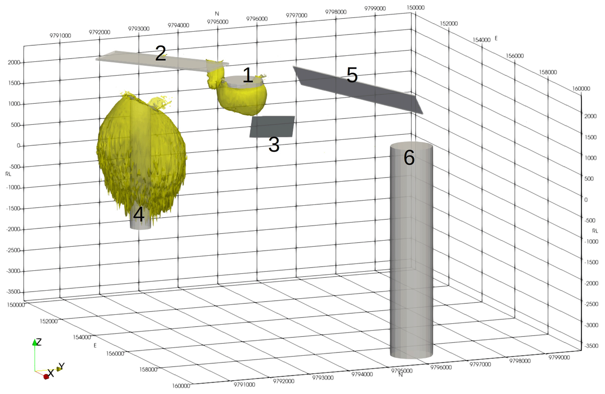
Figure 13 Inverted Synthetic400 magnetisation model. The contours are shown at M = 0.2 A m⁻¹.

Figure 11 shows the memory usage and CPU time (wall time) for compression rates from R_c = 0.1 % to R_c = 50 % for the Callisto model, using N_cpu = 40 cores on a machine with shared memory system. The memory was recorded by the value of “VmHWM” saved in the “/proc/self/status” file. This corresponds to the peak resident set size (“high water mark”) memory. The total memory is calculated by summing up this value across all processors. The memory reported in Fig. 11 is measured at the end of the run to calculate the maximum RAM memory used. Both the memory used and CPU time scale nearly linearly with the compression rate. The theoretical memory prediction Eq.(A1) has a constant offset from the measured memory. This can be explained by the memory internally allocated by the MPI library. The offset also scales nearly linearly with N_cpu, and this is explained by the shared memory allocated by the MPI. Thus, the actual amount of the allocated “offset memory” is smaller than reported using this approach by a factor of ∼ N_cpu.

3.4 Magnetisation inversion example

In this subsection we show a series of two models to test the magnetisation inversion. In the first example we demonstrate the capability of the inversion to recover anomalies. In the second example, we propose a challenging case to evaluate the limits of our code.

3.4.1 Two-body model

In order to test the new magnetisation code, first a simple two-body model was constructed. Each body was only a single model voxel in size. Two cases are considered with (1) both bodies induced and (2) both bodies remanently magnetised with a Koenigsberger ratio of 1. The northern (right-hand) body had its remanence directed almost orthogonal to the inducing field (I_r = 60, D_r = 90 vs. I_i = −60, D_i = 2), and it has a susceptibility of 0.1 SI. The southern (left-hand) body had a susceptibility of 0.05 SI, but its remanent field was parallel to the induced field, which doubled the effective susceptibility. The host had no remanence and a susceptibility of 10⁻⁵ SI. The forward response was computed using both Tomofast-x and UBC's MVIFWD, and good agreement was found for both the TMI and three-component responses. Three-component data were inverted, and the results are shown in Fig. 12. The inverted and true models are in good agreement with respect to anomaly location, magnetisation vector direction, and the relative anomaly magnitude.

3.4.2 Synthetic400 magnetisation model

In order to test the magnetisation code with a more challenging example, the synthetic model described in Sect. 3.1 was revisited, and four of the six bodies had remanence applied to them within the parametric model. Table 4 shows the values used.

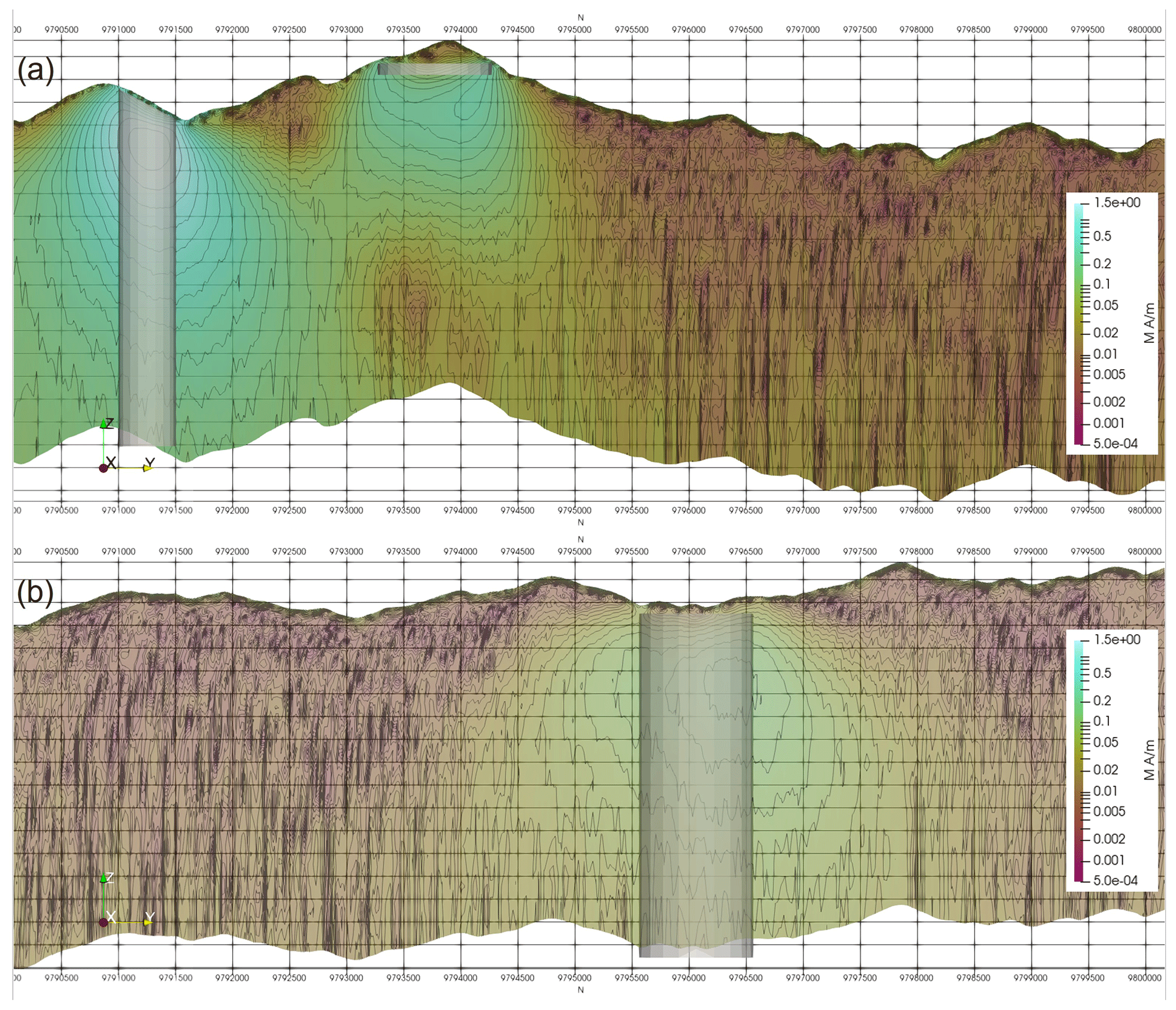
Figure 14 Vertical sections of the inverted Synthetic400 magnetisation model through (a) a high-susceptibility cylinder and disc and (b) a low-susceptibility cylinder.

As before, the computed response from the bodies was added to the response computed for a magnetic half-space with topography, and noise was then added. This was then inverted. Despite moving from solving for one unknown (susceptibility) to three unknowns (magnetisation vector) the inversion has done a good job of identifying the bodies also identified previously, as shown in Fig. 13. The model is smoother than the susceptibility inversion and in the case of the thin sheets and disc the depth is overestimated away from the edges of the sheet or disc. Figure 14a shows a section through the 3D magnetisation model at 154 000E which is through the centre of bodies 4 and 1. When compared with the same section for the susceptibility inversion (Fig. 6a), we note a smoother model and a greater level of sagging below the disc. The low-susceptibility cloak below the disc (body 1) is no longer present, and the background is more homogeneous than was the case for the susceptibility inversion. Looking at the response of the low-susceptibility body (body 6) on section 159 000E (Fig. 14b), we see that the low-susceptibility cylinder is resolved to a local magnetisation high and that the background is more homogeneous than the susceptibility inversion (Fig. 6b).

3.5 Parallel performance tests

We analyse the code parallel performance using two types of machines targeted at different types of users: (1) a single multi-core machine with shared memory system and (2) a large supercomputer with distributed memory across the computational nodes. Most commercial users of the software are likely to use the first type of machine, while academic users are more likely to use the second machine type.

3.5.1 Shared memory tests

The machine used for shared memory tests is an IBM System x3850 X5 server with four Xeon E7-4860 decacore processors running at 2.27 GHz. The machine has 512 Gb of DDR3 (1066) RAM and an Ubuntu 20.04 desktop operating system.

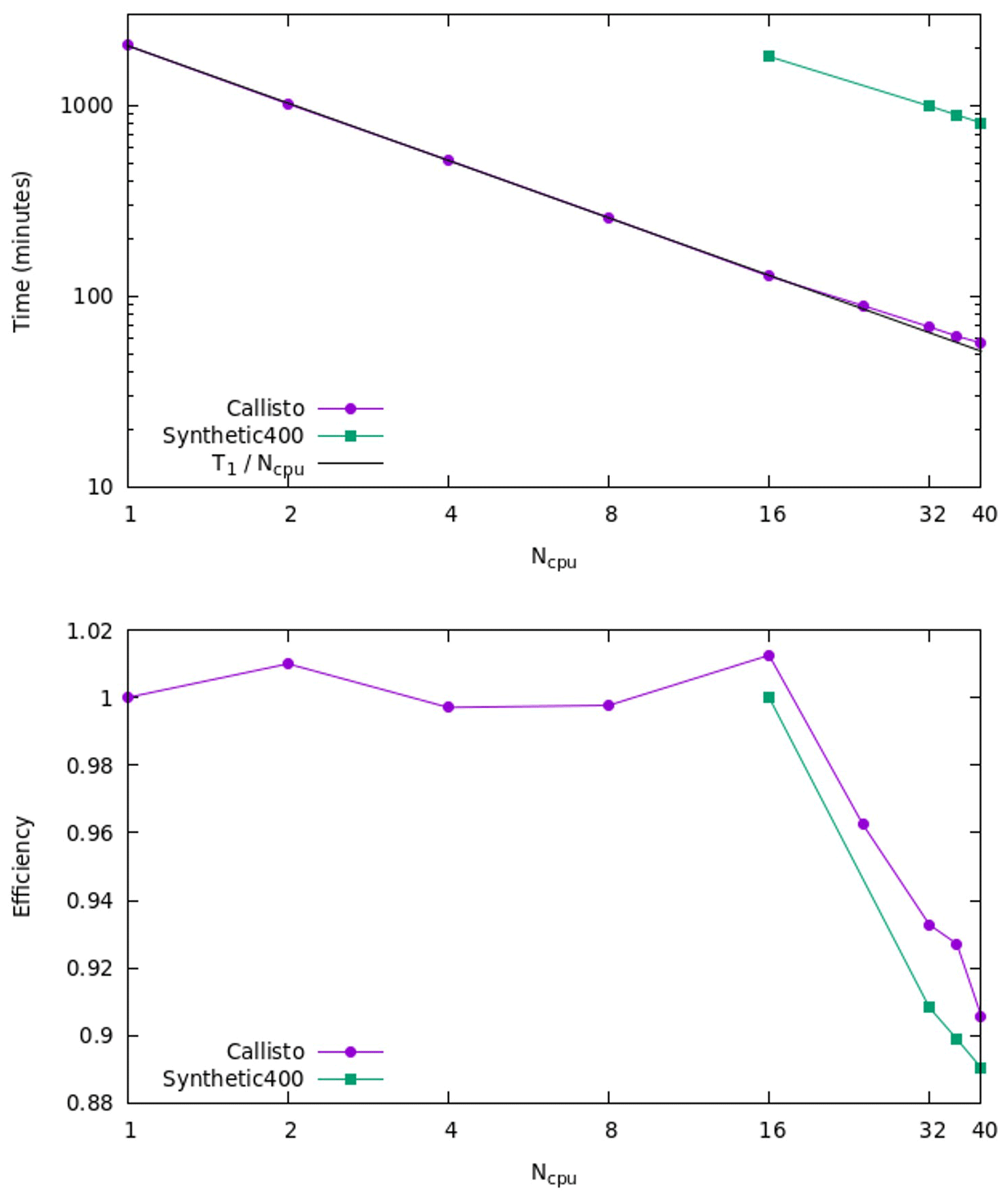
Figure 15 CPU time and parallel efficiency for Callisto and Synthetic400 models for shared memory tests.

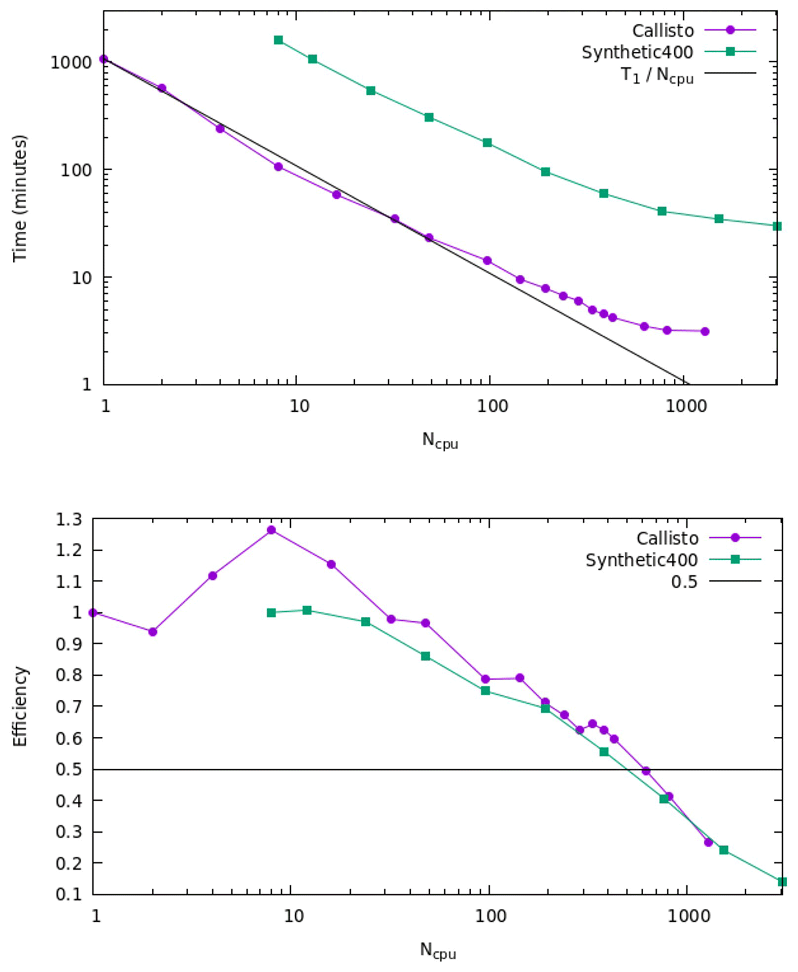
Figure 16 CPU time and parallel efficiency for Callisto and Synthetic400 models for distributed memory tests.

Figure 15 shows the CPU time (wall time) and parallel efficiency for different numbers of MPI processors for the Callisto and Synthetic400 models. The parallelisation efficiency is defined as the ratio of the speedup factor and the number of processors. Note that for the Synthetic400 model the data starting from N_cpu = 16 are shown, as it would take very long time to run it on smaller number of cores; the corresponding parallel efficiency is calculated with respect to N_cpu = 16 for this model. For both models, the CPU time scales nearly linearly with the number of processors up to the maximum number of cores used N_cpu = 40. This is confirmed by high parallel efficiency of greater than ∼ 90 % for all numbers of processors. The nearly linear speed-up with number of processors indicates an efficient use of memory and no sign of bandwidth bottlenecking or I/O limiting performance barriers. It is expected that this would scale to an even higher number of threads, particularly on optically linked distributed memory systems.

To analyse performance, we also measured the MPI time using the Integrated Performance Monitoring tool (IPM). The IPM has an extremely low overhead and is easy to use, requiring no source code modification. Various configurations of MPI settings were tested, and it was found that the strongest impact on the performance has the parameter I_MPI_ADJUST_ALLREDUCE. This controls the algorithm used for the collective MPI communications in the inversion solver. For example, by setting I_MPI_ADJUST_ALLREDUCE = 3, corresponding to “Reduce + Bcast” algorithm, the MPI time for Synthetic400 model was decreased by 25 % on 40 cores. The optimal parameter depends on the machine settings, model size, and the number of cores, and it must be determined experimentally.

3.5.2 Distributed memory tests

For distributed memory tests we use the Gadi supercomputer of the National Computational Infrastructure (NCI), which is Australia's largest research supercomputing facility. Gadi contains more than 250 000 CPU cores, 930 TB of memory, and 640 GPUs. This includes 3074 nodes each containing two 24-core Intel Xeon Scalable “Cascade Lake” processors and 192 GB of memory.

Figure 16 shows the CPU time (wall time) and parallel efficiency for different numbers of MPI processors for the Callisto and Synthetic400 models. Note that for the Synthetic400 model, the data starting from N_cpu = 8 are shown, and the corresponding parallel efficiency is calculated with respect to N_cpu = 8. We observe linear speedup up to N_cpu = 48, as confirmed by parallel efficiency greater than ∼ 95 %. For a higher number of processors, the efficiency is starting to decline, reaching ∼ 80 % at N_cpu = 96 and dropping below 50 % for N_cpu > 624. Overall, through parallelisation, we were able to reduce the total computational time by more than 2 orders of magnitude, achieving maximum speedup of approximately 340 and 420 times for the Callisto and Synthetic400 models, respectively.

4 Discussion and conclusions

Since its initial release in 2021, the Tomofast-x code base has undergone a significant overhaul in terms of both its versatility and performance. Solving for magnetisation rather than susceptibility alone better reflects the real world, where magnetic remanence is much more common than many would like to admit. In addition, allowing input data to have multiple components improves the inverted model relative to a single component inversion of synthetic data, where the answer is known.

Meshes with expanding vertical thickness with depth and matrix wavelet compression have allowed larger problems to be solved in real time. Improvements to the parallelisation scheme have allowed for better performance on both shared and distributed memory systems, with speedups of ∼ 40 and ∼ 400 times, respectively, for moderate-sized models. Memory reduction of up to 100 times is achieved due to wavelet compression of the sensitivity kernel.

Following the changes to the code documented here, Tomofast-x 2.0 produces results very similar to those obtained from the UBC suite of potential field inversion codes. It does so in a similar run time and uses a comparable amount of system resources. However, unlike the commercial version of the UBC suite, it runs on Linux platforms which, because of memory and CPU slot limitations imposed on common versions of the Windows operating system, will allow it to be used on more powerful systems than those typically running Windows. In modern Windows systems it can run on the Windows Subsystem for Linux (WSL) rather than as a Windows application. As maintenance is planned for the foreseeable future, we argue that Tomofast-x can be used for commercial projects and demanding large-scale inversions.

The optimisation work described in this paper is fundamental to allowing more complete descriptions of the controls on magnetisation, including remanence, which require 3 to 9 times the computer resources of the scalar description.

Whilst the modifications described above address many of the challenges of industry and government agencies, further developments are planned, including a closer integration with level set inversions (Giraud et al., 2023a). To extend the gravity to plate-scale problems we would need to reframe the calculations with a spherical coordinate scheme. Increasing use of airborne gravity gradiometry data suggests that including this type of data directly in the inversion scheme also warrants some attention. Finally, and over the longer term, the addition of other types of physics to the platform will have obvious benefits.

Appendix A: Total memory estimation

The total memory requirements for an inverse problem with model damping constraints running in parallel on N_cpu cores has been estimated. The matrix is partitioned by columns (i.e. parallelisation is by model parameters), and single precision floats are used for storing matrix vales. For comparison, both formats (CSR and DCSR) of sparse matrix storage are shown. Note that DCSR format requires less memory on multiple cores due to not having to store the indexes of empty rows. Table A1 shows memory requirement for different types of data structure used in the code.

Table A1 Memory requirements for data structures used in the code.

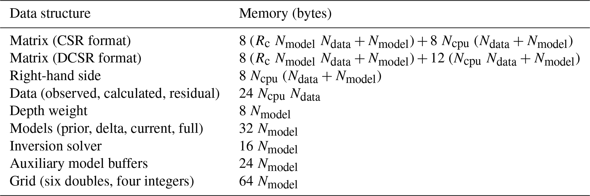
It must be noted that the solver memory is independent of the number of CPUs. To achieve this, the right-hand side vector is used as a buffer for internal solver calculations, and memory allocation for the intermediate products is avoided by using existing memory buffers (for details, see Sect. 2.6). The depth–weight and model arrays are split between the processes, meaning that their memory is independent of the number of cores. Here, the grid memory is allocated only on the master rank to write the final models. The total memory (for the DCSR matrix format) can be estimated as the sum of arrays in Table A1 as follows:

$$\begin{array}{}\text{(A1)}& \begin{array}{rl}{M}_{\text{tot}}=& \mathrm{8}{R}_{\mathrm{c}}{N}_{\text{model}}{N}_{\text{data}}+\mathrm{8}{N}_{\text{cpu}}{N}_{\text{model}}\\ & +\mathrm{44}{N}_{\text{cpu}}{N}_{\text{data}}+\mathrm{164}{N}_{\text{model}}.\end{array}\end{array}$$

This equation can be used to estimate the compression rate, R_c, from the total amount of available memory. It must be noted that the MPI library can allocate additional memory, which is implementation dependent and can vary between different machines.