Structural, petrophysical, and geological constraints in potential field inversion using the Tomofast-x v1.0 open-source code

The quantitative integration of geophysical measurements with data and information from other disciplines is becoming increasingly important in answering the challenges of undercover imaging and of the modelling of complex areas. We propose a review of the different techniques for the utilisation of structural, petrophysical, and geological information in single physics and joint inversion as implemented in the Tomofast-x open-source inversion platform. We detail the range of constraints that can be applied to the inversion of potential field data. The inversion examples we show illustrate a selection of scenarios using a realistic synthetic data set inspired by real-world geological measurements and petrophysical data from the Hamersley region (Western Australia). Using Tomofast-x's flexibility, we investigate inversions combining the utilisation of petrophysical, structural, and/or geological constraints while illustrating the utilisation of the L-curve principle to determine regularisation weights. Our results suggest that the utilisation of geological information to derive disjoint interval bound constraints is the most effective method to recover the true model. It is followed by model smoothness and smallness conditioned by geological uncertainty and cross-gradient minimisation.

1 Introduction

Geophysical data provide detailed information about the structure and composition of the Earth's interior otherwise not accessible by direct observation methods, and thus these data play a central role in every major Earth imaging initiative. Applications of geophysical modelling range from deep Earth imaging to study the crust and the mantle to shallow investigations of the subsurface for the exploration of natural resources. Recent integration of different geophysical methods has been recognised as a means to reduce interpretation ambiguity and uncertainty. Further developments introduce uncertainty estimates from other geoscientific disciplines such as geology and petrophysics to produce more reliable and plausible models. Various techniques integrating different geophysical techniques have been developed with the aim to produce more geologically meaningful models, as reviewed by Parsekian et al. (2015), Lelièvre and Farquharson (2016), Moorkamp et al. (2016), Ren and Kalscheuer (2019), and Meju and Gallardo (2016), and several kinds of optimisation for such problems exist (Bijani et al., 2017). In the natural resource exploration sector, the calls of Wegener (1923), Eckhardt (1940), and Nettleton (1949) for the development of comprehensive, thorough multi-disciplinary and multi-physical integrated modelling have been acknowledged by the scientific community, and data integration is now an area of active research, to quote André Revil's preface of the compilation of reviews proposed by Moorkamp et al. (2016): “The joint inversion of geophysical data with different sensitivities [...] is also a new frontier”. The integration of multiple physical fields (both geophysical and geological) is particularly relevant for techniques relying on potential field gravity and magnetic data, as these constitute the most commonly acquired and widely available geophysical data types worldwide. The need for integrated techniques is partly due to the interpretation ambiguity of geophysical data and resulting effects of non-uniqueness on inversion. Therefore, effective inversion of potential field data necessitates the utilisation of constraints derived from prior information extracted from geological and petrophysical measurements or other geophysical techniques whenever available.

A number of methods for the introduction of geological and petrophysical prior information into potential field inversion have been developed. For example, when limited geological information is available, the assumption is that spatial variation of density and magnetic susceptibility are co-located. This can be enforced through simple structural constraints encouraging structural correlation between the two models using Gramian constraints (Zhdanov et al., 2012) or the cross-gradient technique introduced in Gallardo and Meju (2003). When petrophysical information is available, petrophysical constraints can be applied during inversion to obtain inverted properties that match certain statistics (see techniques introduced by Paasche and Tronicke, 2007; De Stefano et al., 2011; Sun and Li, 2011, 2015, 2016; Lelièvre et al., 2012; Carter-McAuslan et al., 2015; Zhang and Revil, 2015; Giraud et al., 2016, 2017, 2019c; Heincke et al., 2017). Furthermore, when geological data are available, geological models can be derived, and their statistics can be used to derive a candidate model for forward modelling (Guillen et al., 2008; Lindsay et al., 2013; de La Varga et al., 2019), to derive statistical petrophysical constraints for inversion (Giraud et al., 2017, 2019c, d), and to restrict the range of accepted values using spatially varying disjoint bound constraints (Ogarko et al., 2021a) or multinary transformation (Zhdanov and Lin, 2017).

In this paper, we present a versatile inversion platform designed to integrate geological and petrophysical constraints to the inversion of gravity and magnetic data at different scales. We present Tomofast-x (“x” for “extendable”) as an open-source inversion platform capable of dealing with varying amounts and qualities of input data. Tomofast-x is designed to conduct constrained single physics and joint physics inversions. The need for reproducible research (Peng, 2011) is facilitated by open-source code (Gil et al., 2016), and thus we introduce and detail the different constraints implemented in Tomofast-x before providing a realistic synthetic application example using selected functionalities. We illustrate the use of Tomofast-x by performing a realistic synthetic study investigating several modelling scenarios typically encountered by practitioners and provide information to get free access to the source code and to run it using the synthetic data shown in this paper. We perform single physics inversion of gravity data and study the influence of prior information using several amounts and types of constraints, and run joint inversion of gravity and magnetic data. The flexibility of Tomofast-x is exploited to test the effect of structural constraints combined with petrophysical and geological prior information that are yet to be demonstrated in the published literature. A challenging geological setting is used to examine the capability of cross-gradient constraints within the joint inversion method. The mathematical formulations of geophysical problems and solutions are detailed throughout the paper, and sufficient information is provided to allow the reproducibility of this work using Tomofast-x.

The remainder of the contribution revolves around two main aspects. We first review the theory behind the inversion algorithm and the different techniques used, with an emphasis on the mathematical formulation of the problem. We then present a synthetic example inspired from a geological model in the Hamersley province (Western Australia), where we investigate two case scenarios. In the first case, we apply structural constraints to an area where geology contradicts the assumption of co-located and correlated density and magnetic susceptibility variations. In the second case, we investigate a novel combination of petrophysical and structural information to constrain a single physics inversion. Finally, we place Tomofast-x in the general context of research in geophysical inverse modelling and conclude this article.

2 Inverse modelling platform Tomofast-x

2.1 Purpose of Tomofast-x

Tomofast-x can be used in a wide range of geoscientific scenarios as it can integrate multiple forms of prior information to constrain inversion and follow appropriate inversion strategies. Constraints can be applied through Tikhonov-style regularisation of the inverse problem (Tikhonov and Arsenin, 1977, 1978). In single physics inversion, these comprise model smallness (also called “model damping”, minimising the norm of the model; see Hoerl and Kennard, 1970) and model smoothness (also called “gradient damping”, minimising the norm of the spatial gradient of the model; see Li and Oldenburg, 1996). For more detailed imaging, petrophysical constraints using Gaussian mixture models (Giraud et al., 2019c), as well as structural constraints (Giraud et al., 2019d; Martin et al., 2020) and multiple interval bound constraints (Ogarko et al., 2021a), can be used depending on the requirements of the study and the information available. In the case of single physics inversion with structural constraints, structural similarity between a selected reference model and the inverted models can be maximised using structural constraints based on cross-gradients (Gallardo and Meju, 2003) and locally weighted gradients in the same philosophy as Brown et al. (2012), Wiik et al. (2015), Yan et al. (2017), and Giraud et al. (2019d). Generally speaking, in the joint inversion case, the two models inverted for are linked using the structural constraints just mentioned or petrophysical clustering constraints in the same spirit as Carter-McAuslan et al. (2015), Kamm et al. (2015), Sun and Li (2015, 2017), Zhang and Revil (2015), and Bijani et al. (2017). In addition to the underlying assumptions defining the relationship between the properties that have been jointly inverted, prior information from previous modelling or geological information can be incorporated in inversion using model and structural covariance matrices by assigning weights that vary spatially. In such cases, Tomofast-x allows for utilising prior information extensively. Furthermore, Tomofast-x allows the use of an arbitrary number of prior and starting models, enabling the investigation of the subsurface in a detailed and stochastically oriented fashion. Tomofast-x was initially developed for application to regional or crustal studies (areas covering hundreds of kilometres) and retains this capability. The current version of Tomofast-x is now more versatile as development is now directed toward use for exploration targeting and the monitoring of natural resources (kilometric scale).

Lastly, in addition to inversion, Tomofast-x offers the possibility to assess uncertainty in the recovered models. The uncertainty assessments include statistical measures gathered from the petrophysical constraints, posterior least-squares variance matrices of the recovered model (in the least squares with QR-factorisation algorithm – LSQR – sensu Paige and Saunders, 1982; see Sect. 2.5), and the degree of structural similarity between the models (for joint inversion or structurally constrained inversion). From a practical point of view, associated with the inversion algorithm is a user manual covering most functionalities and a reduced 2D Python notebook illustrating concepts (see Sect. 7 for more information) that can be used for testing or educational purposes. A summary of the inverse modelling workflow of Tomofast-x is shown in Fig. 1.

Figure 1 Modelling workflow summary (modified from Jérémie Giraud, Loop Workshop, March 2020).

2.2 General design

The implementation we present extends the original inversion platform “Tomofast” (Martin et al., 2013, 2018). Tomofast-x is an extended implementation proposed and modified by Martin et al. (2018), Giraud et al. (2019c, d), Martin et al. (2020), and Ogarko et al. (2021a). Tomofast-x follows the object-oriented Fortran 2008 standard and utilises classes designed to account for the mathematics of the problem. This introduces enhanced modularity based on the implementation of specific modules that can be called depending on the type of inversion required. The utilisation of classes in Tomofast-x also eases the addition of new functionalities and permits the reduction of software complexity while maintaining flexibility. Our implementation uses an indexed hexahedral solid body mesh, giving the possibility to adapt the problem geometry, allowing the regularisation of the problem in the same fashion as Wiik et al. (2015) or to perform overburden stripping. By default, the sensitivity matrix to geophysical measurements is stored in a sparse format (using the compressed sparse row format) to reduce memory consumption and for fast matrix vector multiplication.

Attention has also been given to computational aspects. The only dependency of Tomofast-x is the message passing interface (MPI) libraries, which eases installation and usage. This allows optimal usage of multi-CPU systems regardless of the number of CPUs. Parallelisation is made on the model cells using a domain decomposition approach in space; i.e. the model is divided into nearly equal, non-overlapping contiguous parts distributed among the CPUs, hence enforcing minimum load imbalance. Consequently, the code is fully scalable as the maximum number of CPUs is not limited by the number of receivers or measured data points. For large 3D models, Tomofast-x can run on hundreds of CPUs for a typical problem with 10⁵–10⁶ model cells and 10³–10⁴ data points. Parallel efficiency tests reveal excellent scalability and speed performance provided that the portions of the model sent to the CPUs are of sufficient size. In the current implementation, the optimum number of elements per CPU is 512. Interested readers can refer to Appendix D for more information.

2.3 Cost function

2.3.1 General formulation

Tomofast-x inversions rely on optimisation of a least-squares cost function and are optimised iteratively. The choice of a least-squares framework was motivated by flexibility in the number of constraints and forms of prior information used in the optimisation process.

The objective function θ is derived from the log likelihood of a probabilistic density function Θ (see Tarantola, 2005, chaps. 1 and 3, for details). In the case of geophysical inversion, it is representative of the “degree of knowledge that we have about the values of the parameters of our system” (Tarantola and Valette, 1982), as summarised below. Let us first define Θ as follows:

$$\begin{array}{}\text{(1)}& \mathrm{\Theta }(\mathit{d},\mathit{m})={\mathrm{\Theta }}_{\mathrm{d}}(\mathit{d},\mathit{m})\prod _{i\in \text{constraints}}{\mathrm{\Theta }}_i\left(\mathit{m}\right),\end{array}$$

where Θ_d(d,m) is the density function over the geophysical data d that model m represents, and Θ_i(m) is the density function for the ith type of prior information available (the “constraints” set).

On the premise that Gaussian probability densities approximate the problem appropriately, Θ_d(d,m) can be expressed as follows:

$$\begin{array}{}\text{(2)}& {\mathrm{\Theta }}_{\mathrm{d}}(\mathit{d},\mathit{m})=A\exp (-\Vert {\mathbf{W}}_{\mathrm{d}}(\mathit{d}-g\left(\mathit{m}\right)\left){\Vert }_{\mathrm{2}}^{\mathrm{2}}\right),\mathrm{A}\in {\mathbb{R}}^{+}\backslash \mathit{\left\{}\mathrm{0}\mathit{\right\}},\end{array}$$

where g(m) is the forward data set calculated by the forward operator g and the matrix W_d weights the data points. Similarly, we formulate the different Θ_{i∈constraints} as follows:

$$\begin{array}{}\text{(3)}& {\mathrm{\Theta }}_i\left(\mathit{m}\right)=C_i\exp (-{\mathit{\alpha }}_i^{\mathrm{2}}\Vert {\mathbf{W}}_i\mathrm{f}(\mathit{m}\left){\Vert }_{\mathrm{2}}^{\mathrm{2}}\right),C_i\in {\mathbb{R}}^{+}\backslash \mathit{\left\{}\mathrm{0}\mathit{\right\}},\end{array}$$

where f is a function of the model and prior information. W_i is a covariance matrix weighting of f(m), and α_i contains positive scalars that are introduced to adjust the relative importance of the ith constraint term. W_i and α_i are derived from prior information or set according to study objectives.

From Eq. (3), it is clear that maximising Θ(d,m) is equivalent to minimising its negative logarithm, θ(d,m), defined as follows:

$$\begin{array}{ll}{\displaystyle }\mathit{\theta }(\mathit{d},\mathit{m})=& {\displaystyle }-\log \mathrm{\Theta }(\mathit{d},\mathit{m})={\mathit{\alpha }}_{\mathrm{d}}^{\mathrm{2}}\Vert {\mathbf{W}}_{\mathrm{d}}(\mathit{d}-g(\mathit{m}\left)\right){\Vert }_{L_{\mathrm{2}}}^{\mathrm{2}}\\ \text{(4)}& {\displaystyle }& {\displaystyle }+\sum _{i\in \text{constraints}}{\mathit{\alpha }}_i^{\mathrm{2}}\Vert {\mathbf{W}}_i\mathrm{f}\left(\mathit{m}\right){\Vert }_{L_{\mathrm{2}}}^{\mathrm{2}},\end{array}$$

which corresponds to the general formulation of a cost function as formalised in the least-squares framework; α_d is a weight controlling the importance of the corresponding data term (i.e. gravity or magnetic) in the overall cost function.

2.3.2 Definition of regularisation constraints

Adapting the formulation of the second term of Eq. (4) to the different types of prior information that we can accommodate leads to the following aggregate cost function:

$$\begin{array}{}\text{(5)}& \begin{array}{rl}& \mathit{\theta }(\mathit{d},\mathit{m})\\ & =\Vert {\mathbf{W}}_{\mathrm{d}}(\mathit{d}-g(\mathit{m}\left)\right){\Vert }_{\mathrm{2}}^{\mathrm{2}}+{\mathit{\alpha }}_{\mathrm{m}}^{\mathrm{2}}\Vert {\mathbf{W}}_{\mathrm{m}}(\mathit{m}-{\mathit{m}}_{\mathrm{pr}}){\Vert }_{\mathrm{p}}^{\mathrm{2}}\\ & +{\mathit{\alpha }}_{\mathrm{g}}^{\mathrm{2}}\Vert {\mathbf{W}}_{\mathrm{g}}\mathrm{\nabla }\mathit{m}{\Vert }_{\mathrm{2}}^{\mathrm{2}}+{\mathit{\alpha }}_{\mathrm{x}}^{\mathrm{2}}\Vert {\mathbf{W}}_{\mathrm{x}}(\mathrm{\nabla }{\mathit{m}}^{\left(\mathrm{1}\right)}\times \mathrm{\nabla }{\mathit{m}}^{\left(\mathrm{2}\right)}){\Vert }_{\mathrm{2}}^{\mathrm{2}}\\ & +{\mathit{\alpha }}_{\text{pe}}^{\mathrm{2}}\Vert {\mathbf{W}}_{\text{pe}}\mathrm{P}\left(\mathit{m}\right){\Vert }_{\mathrm{2}}^{\mathrm{2}}+{\mathit{\alpha }}_{\mathrm{a}}^{\mathrm{2}}\Vert {\mathbf{W}}_{\mathrm{a}}(\mathit{m}-\mathit{z}+\mathit{u}){\Vert }_{\mathrm{2}}^{\mathrm{2}},\end{array}\end{array}$$

where the different terms following the data misfit term $\Vert {\mathbf{W}}_{\mathrm{d}}(\mathit{d}-g(\mathit{m}\left)\right){\Vert }_{\mathrm{2}}^{\mathrm{2}}$ constitute constraints for the inversion of geophysical data acting as regularisation in the fashion of Tikhonov regularisation (Tikhonov and Arsenin, 1977). In Eqs. (2)–(5), W_d represents geophysical data weighting. Generally, W_d should be the data covariance. It is calculated by Tomofast-x as follows:

$$\begin{array}{}\text{(6)}& {\mathbf{W}}_{\mathrm{d}}={\left(\sum _{i=\mathrm{1}}^{n_{\text{data}}}(d_i{)}^{\mathrm{2}}\right)}^{-\mathrm{1}}{\mathbf{I}}_{\mathrm{w}},\end{array}$$

where I_w is a diagonal matrix equal to the identity matrix in single domain inversion or giving the weight of one data misfit term (i.e. gravity data) against the other (i.e. magnetic data) in joint inversion; d_i is the ith datum. By convention, we fix I_w to the identity matrix I for gravity inversion and use I_w=Iα_mag in joint inversion. In such cases, α_mag is a strictly positive scalar.

The main terms of the cost function are defined below. The other individual terms are defined in the next subsection and summarised in Appendix B:

• m_pr refers to the prior model;

• $\Vert {\mathbf{W}}_{\mathrm{m}}(\mathit{m}-{\mathit{m}}_{\mathrm{pr}}){\Vert }_p^{\mathrm{2}}$ represents the smallness term (detailed in Sect. 2.4.1);

• subscript p refers to the L_p norm (here taken such that $\mathrm{1}<p\le \mathrm{2}$);

• ∇ is the operator calculating the spatial gradient of the model;

• $\Vert {\mathbf{W}}_{\mathrm{g}}\mathrm{\nabla }\mathit{m}{\Vert }_{\mathrm{2}}^{\mathrm{2}}$ represents the smoothness constraint on the model (detailed in Sect. 2.4.2);

• $\Vert {\mathbf{W}}_{\mathrm{x}}(\mathrm{\nabla }{\mathit{m}}^{\left(\mathrm{1}\right)}\times \mathrm{\nabla }{\mathit{m}}^{\left(\mathrm{2}\right)}){\Vert }_{\mathrm{2}}^{\mathrm{2}}$ represents cross-gradient constraints between the models m⁽¹⁾ and m⁽²⁾ (detailed in Sect. 2.4.3);

• $\Vert {\mathbf{W}}_{\text{pe}}\mathrm{P}\left(\mathit{m}\right){\Vert }_{\mathrm{2}}^{\mathrm{2}}$ represents petrophysics term (clustering constraint), into which P(m) represents petrophysical distributions used to impose petrophysical constraints (detailed in Sect. 2.4.4);

• $\Vert {\mathbf{W}}_{\mathrm{a}}(\mathit{m}-\mathit{z}+\mathit{u}){\Vert }_{\mathrm{2}}^{\mathrm{2}}$ is the formulation of the multiple bound constraints using the alternating direction of multipliers method (ADMM, detailed in Sect. 2.4.5).

In the case of joint inversion, the vectors defined above are concatenated and the matrices are expanded as follows:

$$\begin{array}{}\text{(7)}& \begin{array}{rl}& g\left(\mathit{m}\right)=\left[\begin{array}{c}{g}_{\mathrm{G}}\left({\mathit{m}}^{\mathrm{G}}\right)\\ g_{\mathrm{M}}\left({\mathit{m}}^{\mathrm{M}}\right)\end{array}\right],\mathit{m}=\left[\begin{array}{c}{\mathit{m}}^{\left(\mathrm{1}\right)}\\ {\mathit{m}}^{\left(\mathrm{2}\right)}\end{array}\right]=\left[\begin{array}{c}{\mathit{m}}^{\mathrm{G}}\\ {\mathit{m}}^{\mathrm{M}}\end{array}\right],\\ & \mathit{d}=\left[\begin{array}{c}{\mathit{d}}_{\mathrm{G}}\\ {\mathit{d}}_{\mathrm{M}}\end{array}\right],\\ & {\mathit{\alpha }}_{i\in \text{[d,m,g,x,pe,a]}}=\left[\begin{array}{cc}{\mathit{\alpha }}_{i\in [\mathrm{d},\mathrm{m},\mathrm{g},\mathrm{x},\mathrm{pe},\mathrm{a}]}^{\mathrm{G}}& \mathrm{0}\\ \mathrm{0}& {\mathit{\alpha }}_{i\in [\mathrm{d},\mathrm{m},\mathrm{g},\mathrm{x},\mathrm{pe},\mathrm{a}]}^{\mathrm{M}}\end{array}\right],\\ & {\mathbf{W}}_{i\in [\mathrm{d},\mathrm{m},\mathrm{g},\mathrm{x},\mathrm{pe},\mathrm{a}]}\\ & =\left[\begin{array}{cc}{\mathbf{W}}_{i\in [\mathrm{d},\mathrm{m},\mathrm{g},\mathrm{x},\mathrm{pe},\mathrm{a}]}^{\mathrm{G}}& \mathbf{0}\\ \mathbf{0}& {\mathbf{W}}_{i\in [\mathrm{d},\mathrm{m},\mathrm{g},\mathrm{x},\mathrm{pe},\mathrm{a}]}^{\mathrm{M}}\end{array}\right],\end{array}\end{array}$$

where T denotes the transpose operator. For the more illustrative purposes of the joint inversion, here we take the gravity and magnetic joint inversion example, where G and M refer to gravity and magnetic problems, respectively.

In the case of single domain inversion, m⁽¹⁾ is the model inverted for and is equal to m^G or m^M depending on the type of geophysical data inverted, and m⁽²⁾ is a reference model that can be used to constrain inversion from a structural point of view (see Sect. 2.4.3, and 4.3 for the theory and an example of utilisation, respectively).

In Eqs. (5)–(7), subscript m, g, x, pe, and a refer to model, gradient, cross-gradient, petrophysics, and ADMM bound constraints, respectively. The different α terms are trade-off parameters that control the importance given to the different terms during the inversion. These terms therefore play an important role in inversion and need to be determined carefully (see Sect. 4.1 and 4.2 for more details).

As mentioned above, the cross-gradient constraints can be applied either to joint or single domain inversion. In the case of ADMM constraints, single or multiple bounds can be applied to define bounds for inverted model values. Such bound constraints can vary in space and be made of an arbitrary number of intervals, regardless of whether they are disjointed or not (see Sects. 2.4.5 and 4.5). Qualitatively, the case with multiple disjoint intervals can be interpreted as applying a dynamic smallness constraint term.

In Tomofast-x, we introduce prior information in the diagonal variance matrices W_i such that they are no longer homogenous and can vary in space. Note that in the implementation of gravity and magnetic inversion, g(m)=Sm, with S the sensitivity matrix relating to measured geophysical data and corresponding recovered physical property (see Appendix C for details about their calculation). Introducing the sensitivity matrix S_G and S_M for gravity and magnetic data, respectively, we obtain the following equation:

$$\begin{array}{}\text{(8)}& g\left(\mathit{m}\right)=\mathbf{S}\mathit{m}=\left[\begin{array}{cc}{\mathbf{S}}_{\mathrm{G}}& \mathrm{0}\\ \mathrm{0}& {\mathbf{S}}_{\mathrm{M}}\end{array}\right]\left[\begin{array}{c}{\mathit{m}}^{\mathrm{G}}\\ {\mathit{m}}^{\mathrm{M}}\end{array}\right]=\left[\begin{array}{c}{g}_{\mathrm{G}}\left({\mathit{m}}^{\mathrm{G}}\right)\\ g_{\mathrm{M}}\left({\mathit{m}}^{\mathrm{M}}\right)\end{array}\right]\end{array}$$

For reference, the terms defined or used here are summarised in Appendix B. Tomofast-x uses the least squares with QR-factorisation (LSQR) algorithm (Paige and Saunders, 1982) to solve the least-squares problem. The full matrix formulation of the problem and the related system of equations are provided in Appendix E.

Generally, not all of the terms in Eq. (5) are used during a single inversion. The activation of selected terms from the cost function (setting α_i>0 and non-null W_i) depends on the information available or on the requirements of the modelling to be performed. For example, a term not used during inversion has the corresponding weighting simply set to 0 (the corresponding matrix W_i is set to 0). Conversely, setting a specific weight to a relatively large value leads to the corresponding constraint to dominate the other terms. Such practice is typically used in sensitivity analysis to examine the effect of incorrectly assigned extreme weighting values on the inversion by providing an example to aid detection of this unintended situation.

In the following subsection, we detail the implementation of the different terms. The terms are introduced and detailed following the order they appear in Eq. (5).

2.4 Detailed formulation of constraints for inversion

In this section, we introduce the mathematical formulation of constraints applied during inversion. Throughout this paper, “geological information” relates to information extracted from probabilistic geological structural modelling. Petrophysical information relates to the statistics of the values inverted for (density contrast and magnetic susceptibility).

2.4.1 Smallness term

We repeat the smallness term as follows:

$$\begin{array}{}\text{(9)}& \Vert {\mathbf{W}}_{\mathrm{m}}(\mathit{m}-{\mathit{m}}_{\mathrm{pr}}){\Vert }_p^{\mathrm{2}}.\end{array}$$

The smallness term corresponds to the ridge regression constraint, i.e. the smallness term of Hoerl and Kennard (1970). To simplify the problem, the covariance matrix W_m is assumed to be a diagonal matrix. In Tomofast-x, it is used to adjust the strength of the constraint either globally (i.e W_m=I) or locally (i.e. the elements of W_m may vary from one cell to another). In the second case, W_m can be determined using prior information such as uncertainty from geological modelling or models and structural or statistical information derived from other geophysical techniques (e.g. seismic attributes and probabilistic results from magnetotellurics).

2.4.2 Smoothness term

The smoothness model term (Li and Oldenburg, 1996) is a total variation (TV)-like regularisation term based on an original idea of Rudin et al. (1992). It constrains the degree of structural complexity allowed in the inverted model. We repeat the term as follows:

$$\begin{array}{}\text{(10)}& \Vert {\mathbf{W}}_{\mathrm{g}}\mathrm{\nabla }\mathit{m}{\Vert }_{\mathrm{2}}^{\mathrm{2}}.\end{array}$$

The covariance matrix W_g modulates the importance of the term by assigning the weights to each cell. For the sake of simplicity, the matrix W_g is commonly assumed to be a diagonal matrix. It is commonly set as the identity matrix (W_g=I), but several works vary the values in space accordingly with prior information. For instance, Brown et al. (2012) and Yan et al. (2017) use seismic models to calculate such weights for the inversion of electromagnetic data, and Giraud et al. (2019a), who present an application case using Tomofast-x, invert gravity data using geological uncertainty information to calculate W_g. In Tomofast-x, it can be set either globally (i.e. W_g=I) or locally (i.e. the elements of W_g may vary from one cell to another).

2.4.3 Cross-gradient

The cross-gradient constraints were introduced as a means to link two models that are inverted jointly by encouraging structural correlation between them (Gallardo and Meju, 2004). We refer the reader to Meju and Gallardo (2016) for a review of applications using this technique. We repeat the term below:

$$\begin{array}{}\text{(11)}& \Vert {\mathbf{W}}_{\text{x}}(\mathrm{\nabla }{\mathit{m}}^{\left(\mathrm{1}\right)}\times \mathrm{\nabla }{\mathit{m}}^{\left(\mathrm{2}\right)}){\Vert }_{\mathrm{2}}^{\mathrm{2}}.\end{array}$$

The matrix W_x modulates the importance of the term by assigning the weights to each cell. In previous works, it is always (to the best our knowledge) set as the identity matrix (W_x=I), with the exception of Rashidifard et al. (2020), who define such weights using seismic reflectivity and apply this approach to single physics inversion of gravity data constrained by fixed seismic velocity. In Tomofast-x, three finite-difference numerical schemes can be chosen to calculate the cross-gradient derivatives: forward, centred, and mixed. In what follows, we use a “mixed” finite-difference scheme, where inversion iterations with an odd number use a forward scheme and those with even numbers use a backward scheme (e.g. iteration 3 will use a forward scheme and iteration 4 a backward scheme). This scheme was chosen as it reduces the influence of the border effects of both the forward and backward schemes on the inverted model.

2.4.4 Statistical petrophysical constraints

One strategy to enforce the petrophysical constraints using statistics from petrophysical measurements is performed by encouraging the statistics of the recovered model to match that of a statistical model derived either from measurements made from the study area or literature values. In the current implementation of Tomofast-x, a mixture model representing the expected statistics of the modelled rock units is used. We use a Gaussian mixture model to approximate the petrophysical properties of the lithologies in the studied area. In the mixture model, the weight of each Gaussian can be set in the input. We suggest using the probability of the corresponding rock unit when this information is available. The mismatch between the statistics of the recovered model and the mixture model is minimised in the optimisation framework following the same procedure described in Giraud et al. (2018, 2019b).

In the ith model cell, the likelihood term P(m_i) of model cell m_i is calculated as follows for the kth lithology:

$$\begin{array}{}\text{(12)}& {\displaystyle }{\mathcal{N}}_k& {\displaystyle }={\mathit{\omega }}_k\mathcal{N}(m_i\mathrm{|}{\mathit{\mu }}_k,{\mathit{\sigma }}_k)\text{(13)}& {\displaystyle }\mathrm{P}\left(m_i\right)& {\displaystyle }=-\log \left(\sum _{k=\mathrm{1}}^{n_{\mathrm{f}}}{\mathcal{N}}_k\right)+\log (max{\mathcal{N}}_{k=\mathrm{1}\mathrm{\dots }{n}_{\mathrm{f}}}),\end{array}$$

where

$$\begin{array}{}\text{(14)}& \left\{\begin{array}{ll}{\mathit{\omega }}_k=\frac{\mathrm{1}}{n_{\mathrm{f}}}& \text{everywhere in the absence of spatially-}\\ & \text{varying prior information (a)}\\ {\mathit{\omega }}_k={\mathit{\psi }}_{k,i}& \text{in the }i\text{th cell using prior information (b)},\end{array}\right.\end{array}$$

𝒩 symbolises the normal distribution, and n_f is the total number of rock formations observed in the modelled area.

In practice, an expectation maximisation algorithm (McLachlan and Peel, 2000) can be used to estimate the mean μ_k and standard deviation σ_k of the petrophysical measurements.

In Eqs. (12)–(14), ω_k is the weight assigned to the Gaussian distribution representative of the petrophysics of the kth lithology in the mixture. In Eq. (14a), the weight ω_k assigned to each lithology is constant across the model, while in Eq. (14b) the weight ψ_k,i is derived from information derived from another modelling technique (geology, seismic, electromagnetic methods, etc.) and varies spatially.

We note that a small number of Gaussian distributions might not be suitable to approximate certain types of distributions like bimodal (magnetic susceptibility) or lognormal (electrical resistivity) distributions. However, we point out that increasing the quality of such an approximation depends on the number of Gaussian distributions used for approximation (McLachlan and Peel, 2000).

2.4.5 Disjoint bound constraints using the ADMM algorithm

The objective of the disjoint bound constraints is to optimise Eq. (5) while ensuring that in every model cell $m_{\mathrm{1}\le i\le n_{\mathrm{m}}}$ the inverted value lies within the prescribed bounds such that m_i∈B_i, defined as follows (Ogarko et al., 2021a):

$$\begin{array}{}\text{(15)}& B_i=\bigcup _{l=\mathrm{1}}^{L_i}[a_{i,l},b_{i,l}],\text{with}{b}_{i,l}>a_{i,l},\forall l\in [\mathrm{1},L_i],\end{array}$$

where a_i,l and b_i,l are the lower and upper bounds for the ith model cell and l is the lithology index; L_i≤n_f is the total number of bounds allowed for the considered cell, corresponding to the number of distinct rock units allowed by such constraints. During inversion, such multiple bound constraints on the physical property values inverted for are gradually enforced using the ADMM algorithm. Implementation details are beyond the scope of this paper, but more information is provided in Appendix E, and we refer the reader to Ogarko et al. (2021a) for details. Details about the general mathematical formulation of the ADMM algorithm can be found in Dykstra (1983), chap. 7 in Bertsekas (2016), and in Boyd et al. (2011).

Note that the application of the ADMM bound constraints can be interpreted as being analogous to clustering constraints where (taking the example of the kth model-cell) the following conditions are met:

1. the centre values depend on both the current model m at any given integration and petrophysical information defining a and b;

2. the weight assigned to each centre value changes from one iteration to the next as a function of the distance between m_k and the closest bound, and the number of iterations m_k has remained outside B_k.

2.4.6 Depth weighting and data weighting

To balance the decreasing sensitivity of potential field data with the depth of the considered model cell, Tomofast-x offers the possibility for the calculation of the depth-weighting operator. The first one, which we use in this paper, utilises the integrated sensitivities technique following Portniaguine and Zhdanov (2002). For each model cell i, a weight D_ii is introduced:

$$\begin{array}{}\text{(16)}& D_{ii}={\left(\sum _{k=\mathrm{1}}^{n_{\text{data}}}(S_{ki}{)}^{\mathrm{2}}\right)}^{\frac{\mathrm{1}}{\mathrm{4}}}.\end{array}$$

The second option relies on the application of an inverse depth-weighting power law function following Li and Oldenburg (1998) and Li and Chouteau (1998) for gravity and Li and Oldenburg (1996) for magnetic data:

$$\begin{array}{}\text{(17)}& D_{ii}={\left({\displaystyle \frac{\mathrm{1}}{z_i+\mathit{\epsilon }}}\right)}^{\mathit{\beta }},\end{array}$$

where z_i is the depth of the ith model cell and ε is introduced to ensure numerical stability, such that z≫ε; the value of β depends on the type of data considered (gravity or magnetic). For more details about the use of depth weighting and selection of values of β, the reader is referred to the references provided in this subsection. The application of depth weighting as a preconditioner to the matrix system of equation solved for during inversion is shown in Appendix E.

2.5 Posterior uncertainty metrics

Uncertainty information is an important building block of modelling and a critical aspect of decision making (Scheidt et al., 2018). When available, uncertainty information can be communicated and used in subsequent modelling or for decision making (see examples of Ogarko et al., 2021a, who use uncertainty information in the model recovered by another method as input to their modelling using Tomofast-x). Tomofast-x allows the calculation of metrics reflecting the degree of uncertainty in the models before and after inversion. It allows monitoring the evolution of the different terms of the cost function during inversion. Tomofast-x also calculates uncertainty metrics that are specific to the kind of constraints used in inversion:

• the posterior covariance matrix of model m as estimated by the LSQR algorithm (Paige and Saunders, 1982, p. 53, for details and Sect. A1.1 for a brief introduction),

• the value of the cross-gradient in each cell,

• the individual 𝒩_k values (Eq. 12) of the different Gaussians making up the Gaussian mixture used to define the petrophysical constraints.

The implementation of this series of indicators was performed with the intent to provide metrics for posterior analysis in detailed case studies. More information about these posterior uncertainty indicators is provided in Appendix A, which details functionalities of Tomofast-x not explored here.

3 Synthetic model and data

In this section, we introduce how the data used for synthetic modelling were derived, and we present examples of using prior information derived from geological modelling. The process of simulating a realistic field case study is described with the design of the numerical experiment.

3.1 Geological framework

The original geological model is based on a region in the Hamersley province (Western Australia). It was built using the map2loop algorithm (Jessell et al., 2021b) to parse the raw data and the Geomodeller^® implicit modelling engine for geological interpolation (Calcagno et al., 2008; Guillen et al., 2008) to model the contacts, stratigraphy, and orientation data measurement in the area (see the geographical location in Fig. 2). Data used to generate the model comprise the 2016 1:500 000 Interpreted Bedrock Geology map of Western Australia (https://catalogue.data.wa.gov.au/dataset/1-500-000-state-interpreted-bedrock-geology-dmirs-016, last access: 2 December 2020) and the WAROX outcrop database (https://catalogue.nla.gov.au/Record/7429427, last access: 2 December 2020). Geological modelling was assisted by interpretation of the magnetic anomaly grid compilations at 80 m and the 400 m gravity anomaly grid from the Geological Survey of Western Australia (https://www.dmp.wa.gov.au/Geological-Survey/Regional-geophysical-suvey-data-1392.aspx, last access: 2 December 2020). More information about data availability is provided in Sect. 7.

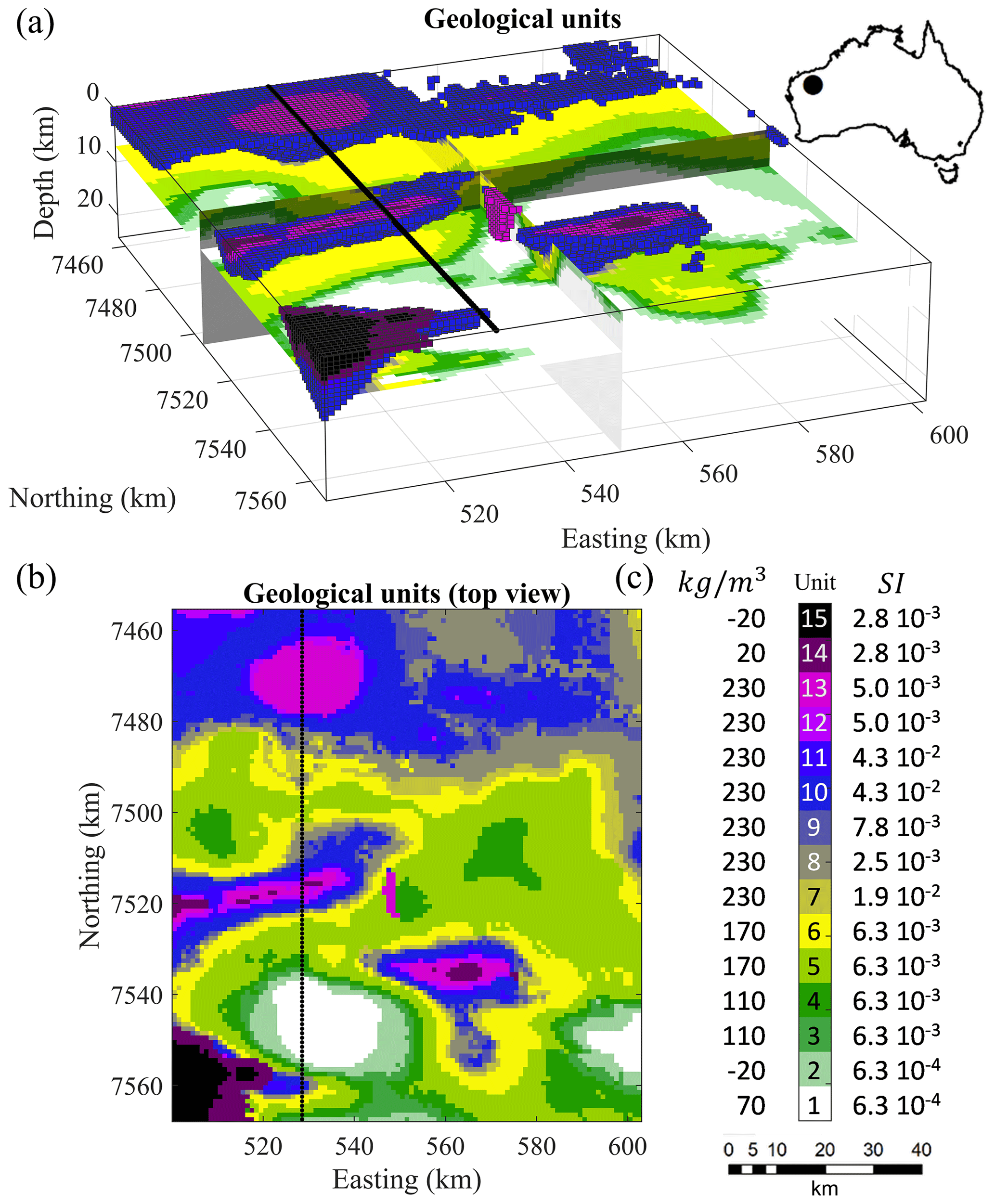
Figure 2 True model used for geologic modelling and geophysical inversion. The top panel shows the map view. The black line represents the surface coordinates of the 2D profile considered here for illustration of Tomofast-x's utilisation. The values given on either side of the colour bar indicate the density contrast and magnetic susceptibility attached to each rock unit. Note that several rock units present similar density contrast or magnetic susceptibilities, making them undistinguishable using either gravity or magnetic inversion.

In what follows, we use an adapted version of the original structural geological framework of the selected region by increasing the vertical dimensions of the model cells and assuming a flat topography. The resulting reference geological model used to generate the physical properties for geophysical modelling measurements is shown in Fig. 2 in terms of its geological units.

In addition to the modification of the structural model, we make adjustments to the original density values derived from field petrophysical measurements by reducing the differences between the density contrasts of different rock units. By doing so, we increase the interpretation ambiguity of inversion results and decrease the differentiability of the different rock units. The same procedure is applied to magnetic susceptibility to make accurate imaging using inversion more challenging. The three-dimensional (3D) density contrast and magnetic susceptibility models used to generate the gravity and magnetic data are shown in Fig. 3.

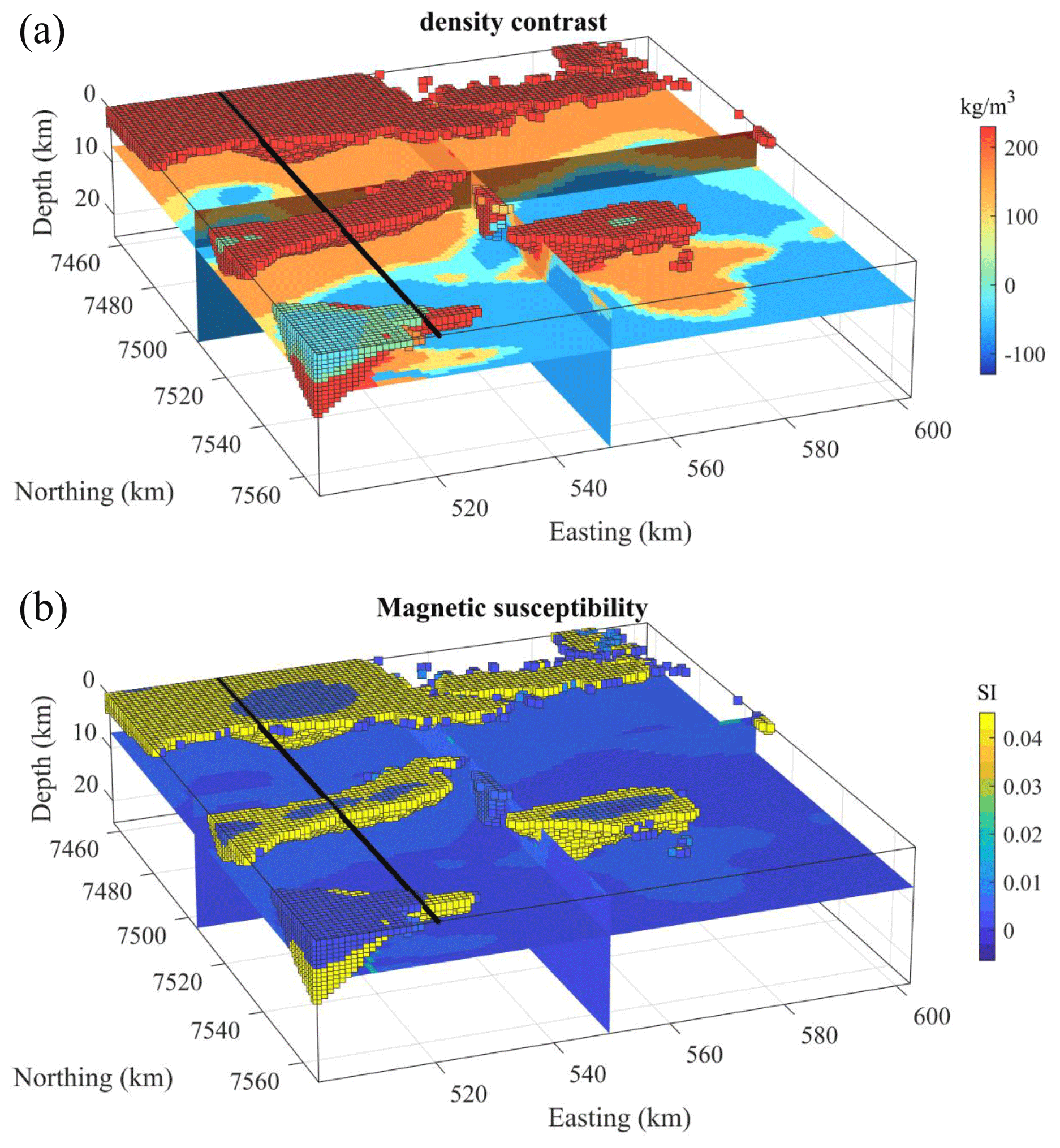
Figure 3 True synthetic density contrast (a) and magnetic susceptibility (b) model used for the simulation of geophysical data. The black line represents the surface coordinates of the 2D profile considered here. The voxels represent lithologies 10 through 15, colour-coded with their respective density contrast and magnetic susceptibility values.

3.2 Geophysical simulations and model discretisation

The core 3D model is discretised into $N_{\mathrm{x}}\times N_y\times N_z=\mathrm{103}\times \mathrm{113}\times \mathrm{33}$ cells of dimensions equal to $\mathrm{999}\times \mathrm{996}\times \mathrm{745}$ m³. For both gravity and magnetics, we generate one geophysical measurement per cell along the horizontal axis, leading to $N_{\mathrm{x}}\times N_y=\mathrm{11}\mathrm{639}$ data points for each method, and add 10 padding cells in each horizontal direction to limit numerical border effects in the forward calculation, leading to a total of $\mathrm{123}\times \mathrm{133}\times \mathrm{33}=\mathrm{539}\mathrm{847}$ model cells. We simulate a ground gravity survey by locating the measurements 1 m above ground level, and aeromagnetic data acquired by a fixed-wing aircraft flying 100 m above surface. To test the robustness of our inversion code to noise content in the data, the geophysical data inverted here are contaminated by noise.

The noise component was generated as follows. For each gravity measurement, we first add a perturbation value randomly sampled from the standard normal distribution of the whole data set multiplied by 9 % of the measurement's amplitude. We then add a second perturbation value randomly sampled from the standard normal distribution with an amplitude of 3 mGal (2 % of the dynamical range). These values were derived manually to obtain a realistic noise contamination. To simulate small-scale spatial coherence in the noise generated in this fashion, we then apply a two-dimensional Gaussian filter to the 2D noise map obtained from the previous step. We then apply a two-dimensional median filter to the resulting noise-contaminated gravity data to simulate de-noising. For magnetic data, we apply the same procedure, using 12.5 % of the measurement's amplitude for the first step and 15 nT (1 % of the dynamical range) for the second step. Similarly to gravity data, these values were derived manually; no levelling noise was simulated. For comparison, the noise-free and contaminated synthetic measurements are shown in Fig. 4. The resulting noise standard deviation σ_noise for gravity and magnetic data are equal to 1.2 mGal and 8.5 nT, respectively.

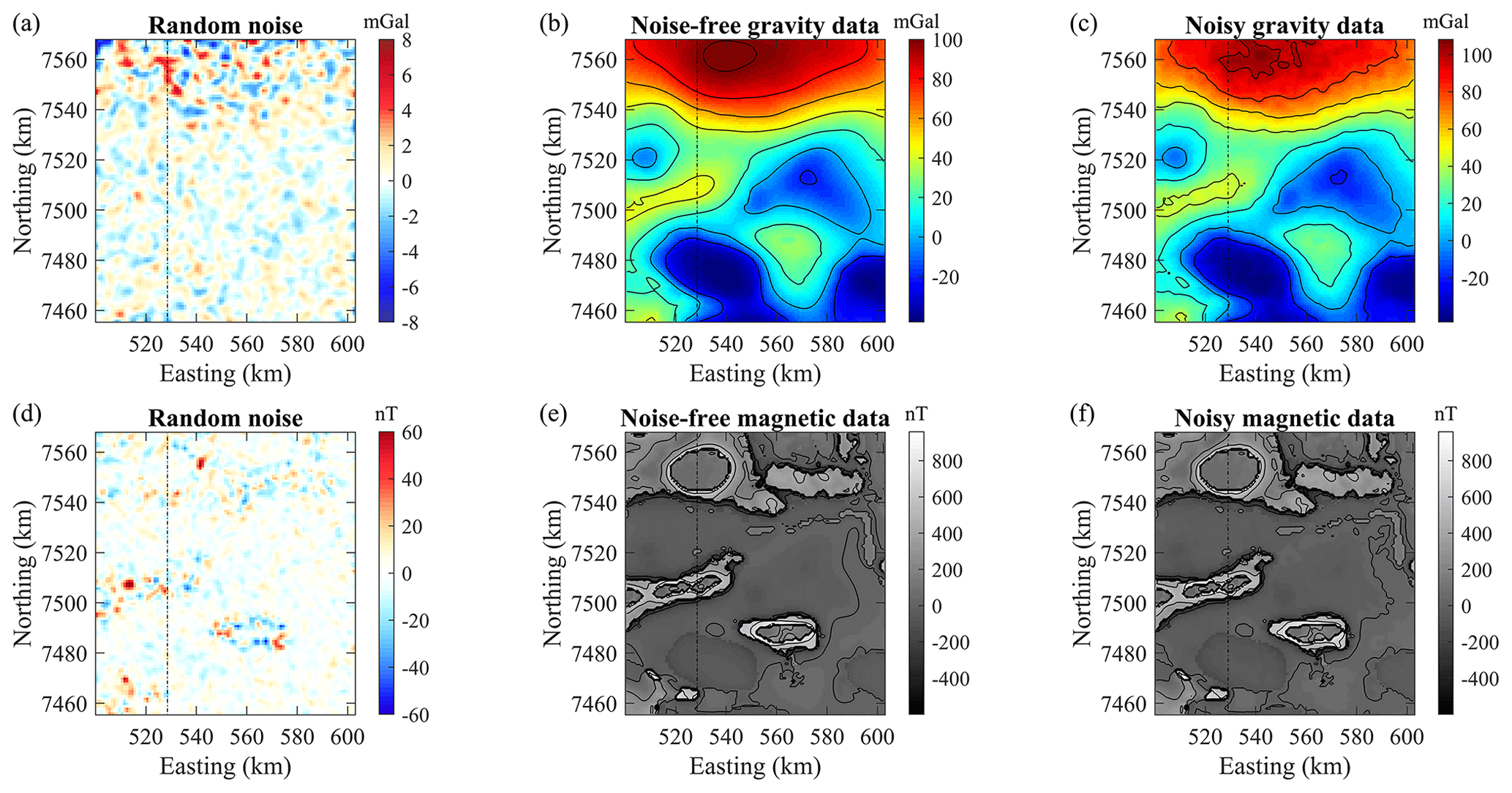
Figure 4 Noise (a, d) added to the data calculated from the true model (b, e) and resulting noisy data (c, f) for the gravity (a–c) and magnetic (d–f) data sets. The contour lines shown correspond to the ticks shown in the palette's colour bar. The black line represents the location profile we use for the inversions performed here.

The gravity data modelled here correspond to the complete Bouguer anomaly. Magnetic data are simulated using the magnetic strength of the Hamersley province (53 011 nT, which approximates the International Geomagnetic Reference Field in the area) reduced to the pole.

To complete the 3D modelling procedure, a series of 100 structural geological models are generated using Monte Carlo perturbations of the geological measurements (foliation and contact points between geological units) constraining the geological structures. This was performed using the Monte Carlo Uncertainty Estimator (MCUE) technique of Pakyuz-Charrier et al. (2018, 2019). The result is an ensemble of models that all fit the geological measurements within a given set of prior uncertainty parameters. The ensemble is thus assumed to represent the geological model space, rather than just a single “best-guess” model. Probabilities for the occurrence of different rock units can be calculated from the ensemble and used to constrain geophysical inversion (see examples of Giraud et al., 2017, 2019a; Ogarko et al., 2021a). More specifically, MCUE is useful to obtain the probability ψ_i,l of occurrence of the different lithologies l for every ith model cell and to calculate the related uncertainty indicators (Sect. 3.3). Detailing the probabilistic geological modelling procedure and analysing the results in 3D is beyond the scope of this paper and interested readers are referred to Lindsay et al. (2012), Pakyuz-Charrier et al. (2018), Wellmann and Caumon (2018), and references therein.

In this contribution, we simulate a case study where modelling is carried out along the 2D profile materialised by the black line in Figs. 3 and 4, extracted from the 3D modelling framework as detailed in the next subsection.

3.3 2D model simulation in a 3D world

As mentioned above, we perform the inversion of geophysical data along a 2D profile for simplicity and to simulate the challenging case of 2D data acquired in a 3D geological setting, in a part of the model where subhorizontal or gently dipping features can be observed. The philosophy of the numerical study presented here is summarised in Fig. 5.

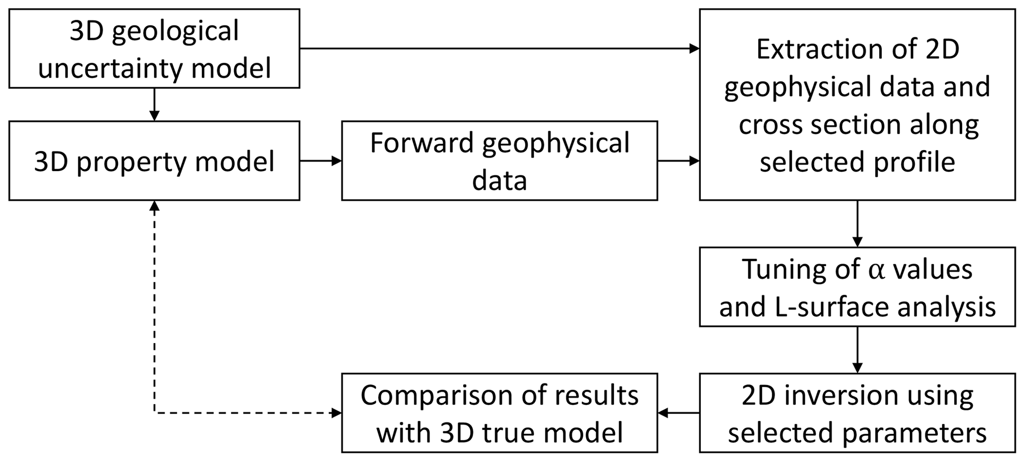
Figure 5 Summary of experimental protocol for synthetic study and testing of different functionalities of Tomofast-x.

The 2D geological Sect. considered is shown in Fig. 6 (the black line marked in Figs. 3 and 4). Geological certainty is estimated using a measure of the dispersion away from the perfectly uninformed case where the all rock units are equiprobable. In each model cell, this measure, which we write as ${\mathit{\sigma }}_{\mathit{\psi }}^{\prime }$, is calculated as a function of the standard deviation σ_ψ of the probability ψ of observing the different rock units as follows:

$$\begin{array}{}\text{(18)}& {\mathit{\sigma }}_{\mathit{\psi }}^{\prime }=\sqrt{\mathrm{1}/\text{card}}-{\mathit{\sigma }}_{\mathit{\psi }},\end{array}$$

where card is the geological cardinality of the model. It is equal to the number of possible rock units observed in one location across the entire ensemble. From Eq. (18), ${\mathit{\sigma }}_{\mathit{\psi }}^{\prime }$ is maximum where rock units are well constrained and minimum where the model is the most uncertain. This geological certainty metric is shown in Fig. 6 for the 2D section considered in this example.

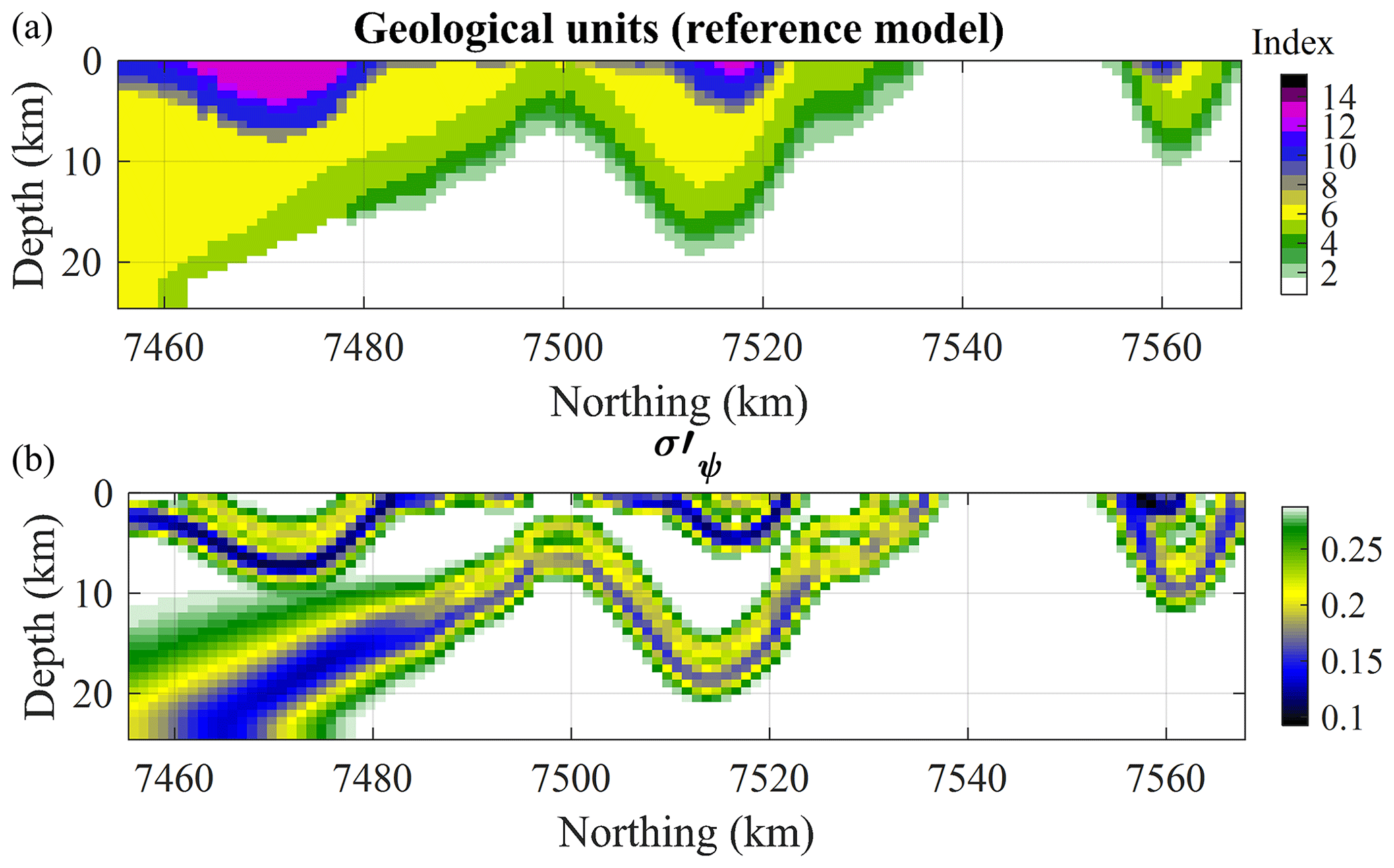
Figure 6 Two-dimensional slice extracted from the 3D model along the profile: geological reference model (a) and the ${\mathit{\sigma }}_{\mathit{\psi }}^{\prime }$ metric (b). Here, the geological uncertainty metric considered is the standard deviation of the probability of the different lithologies as per Eq. (18).

The probabilities of observation of the different lithologies are shown in Fig. 7. Note that for the purpose of the tests we perform on gravity data inversion, we reduce the set of probabilities by grouping rock units into fictitious units with the same density contrasts as single rock units. This reduces the number of rock units to six units that can be distinguished by gravity inversion, as several units may be assigned the same density contrast.

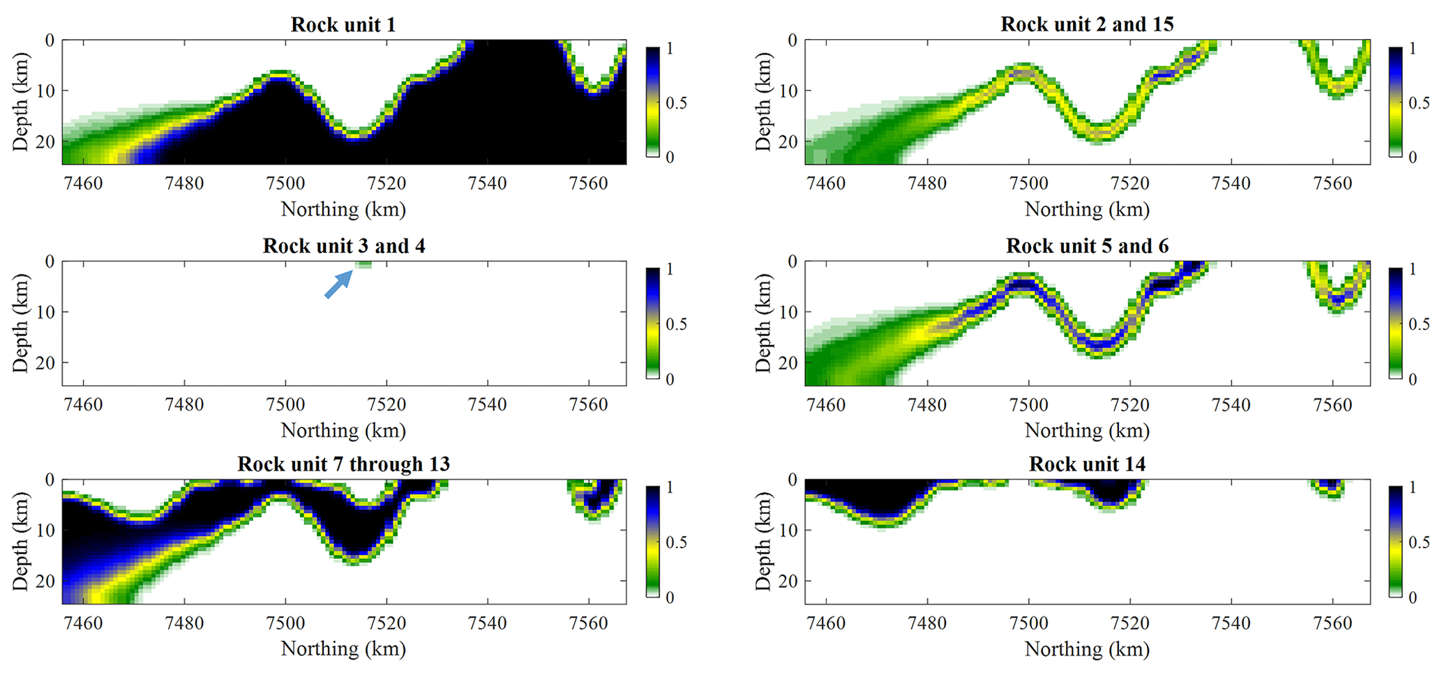
Figure 7 Observation probabilities for the rock units that present differencing density contrasts. Units 3 and 4 are nearly absent from the section (see maximum probability area marked by the arrow).

The geophysical data we use for inversion are extracted along the line marked in Figs. 3 and 4. The geophysical data and reference (true) petrophysical model extracted in this fashion are shown in Fig. 8. Care was taken not to use the same mesh for both generating the synthetic data set and its inverse modelling.

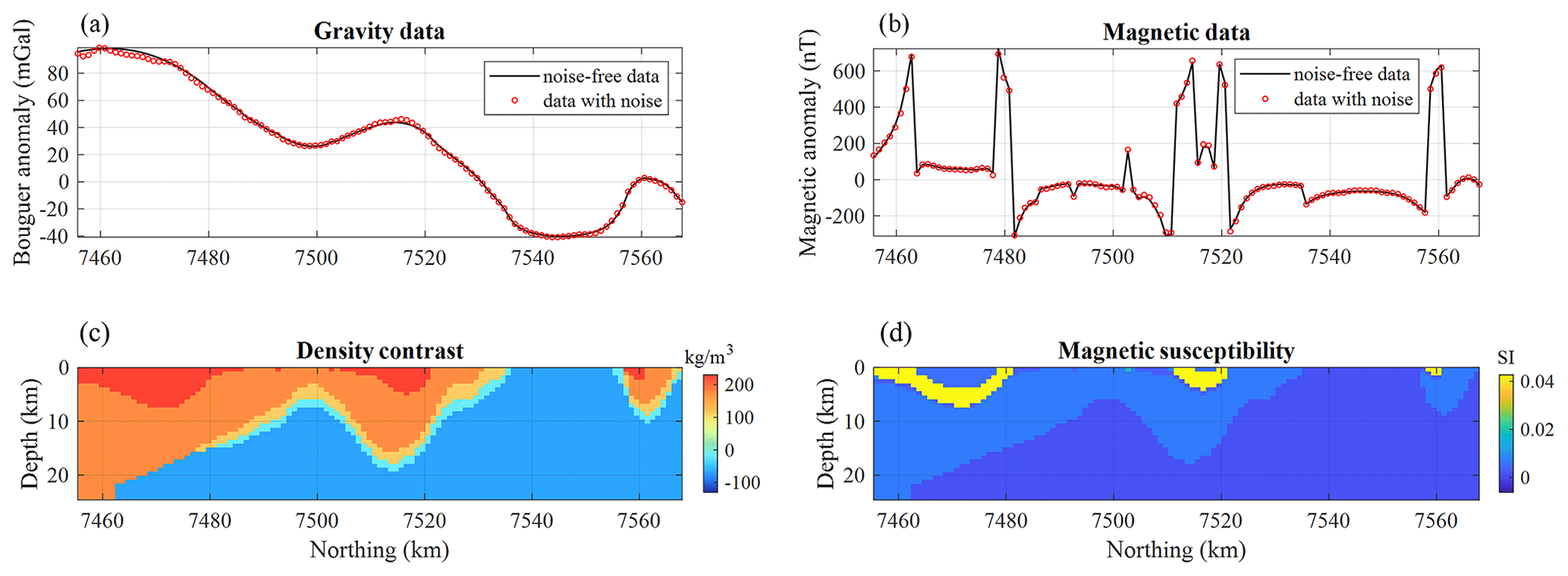
Figure 8 Two-dimensional slice extracted from the 3D model: gravity data and density contrast (a) and magnetic data and magnetic susceptibility (b).

To inverse model the data shown in Fig. 8, we generate a mesh centred on the profile (oriented along the y direction) and add padding to either side and the northern and southern extremities. The resulting model comprises $n_{\mathrm{x}}\times n_y\times n_z=\mathrm{13}\times \mathrm{133}\times \mathrm{33}$ cells of dimensions equal to $\mathrm{2998}\times \mathrm{996}\times \mathrm{745}$ m³. Note that we increased the model cell size in the direction perpendicular to the profile. The gravity and magnetic data sets along the profile each comprise 113 data points evenly distributed along the line.

While we focus on a 2D section extracted from a 3D model presented here (see location in Figs. 3 and 4), the 3D model and the associated gravity and magnetic data sets shown here are made publicly available (see Sect. 7).

4 Application example: sensitivity analysis to constraints and prior information

In the examples shown below, we first perform single domain and joint (multiple domain) inversion (using the cross-gradient constraint) assuming identity matrices for W_m, W_g, and W_x. We then investigate the influence of prior information on single domain inversion by combining structural and petrophysical information in the case of gravity inversion. The combination of petrophysical and structural constraints derived from geology is tested. The intention is to address knowledge gaps in the literature that describe the effects of parameterisation of such constraints.

4.1 Experimental protocol

It is necessary to determine the appropriate weights α assigned to the terms defining the constraints applied during inversion to optimise the cost function in Eq. (5). The α values that define the weights of the different terms in the cost function constitute hyperparameters of the inverse problem. Appropriate estimation of these hyperparameters is necessary to approximate the optimum value of the global misfit function. To this end, we use the L-curve principle (Hansen and O'Leary, 1993; Hansen and Johnston, 2001; Santos and Bassrei, 2007) for each of the cases presented below. We perform series of inversions, sampling α values spanning the plausible range of potential choices using a heuristic approach.

When two constraint terms are used in inversion (i.e. with α>0), we extend the L-curve approach to the two-parameter cases. In such cases, the optimum values for the α weights are determined by applying the L-curve criterion using L-surfaces (or elbow surface) instead of L-curves (Belge et al., 2002) (we note that the L-curves as plotted here can also be referred to as “Tikhonov curves” in the case where data misfit is plotted as a function of regularisation value). The optimum value for the α weight of the two constraint terms is therefore obtained by identification of the inflection point of the surface made up of the variations of the data misfit as a function of the weights under consideration. We chose this approach for its simplicity and note that there exist other techniques that use an automated process, such as the generalised cross-validation technique (Craven and Wahba, 1978). We refer the reader to Farquharson and Oldenburg (2004) for a general introduction and Giraud et al. (2019b) and Martin et al. (2020) for an application of this principle to inversions using Tomofast-x. The role the L-surface analysis plays in the synthetic case presented here is reminded in the workflow shown in Fig. 5. In our analysis, we set the objective value for the data misfit $\Vert {\mathbf{W}}_{\mathrm{d}}(\mathit{d}-g(\mathit{m}\left)\right){\Vert }_{\mathrm{2}}^{\mathrm{2}}$ to be equal to the objective data misfit ${\mathrm{\Theta }}_{\mathrm{d}}^{\text{obj}}(\mathit{d},\mathit{m})$, defined as follows:

$$\begin{array}{}\text{(19)}& {\mathrm{\Theta }}_{\mathrm{d}}^{\text{obj}}(\mathit{d},\mathit{m})\ge {\displaystyle \frac{n_{\text{data}}{\mathit{\sigma }}_{\text{noise}}}{{\sum }_{i=\mathrm{1}}^{n_{\text{data}}}(d_i{)}^{\mathrm{2}}}},\end{array}$$

so that the data is reproduced with a level of error superior or equal to the estimated noise level of the data. Here, this leads to ${\mathrm{\Theta }}_{\mathrm{d}}^{\text{obj}}=\mathrm{5.01}\times {\mathrm{10}}^{-\mathrm{4}}$ for gravity inversion and to ${\mathrm{\Theta }}_{\mathrm{d}}^{\text{obj}}=\mathrm{1.55}\times {\mathrm{10}}^{-\mathrm{4}}$ for magnetic data inversion.

For the sake of consistency in our study of the influence of constraints on inversion, we set m_pr=0 kg m⁻³ for gravity data inversion and m_pr=0 SI for magnetic data inversion.

4.2 Homogenously constrained potential field inversions

We first perform single physics inversion following the common strategy of constraining the model using smallness and smoothness constraints. Obtaining a good approximation of the optimum values of these parameters gives insights into the numerical structure of the problem. It constitutes valuable knowledge when using other kinds of constraints, and we consider it good practice to run such inversion prior to using more advanced constraints. Here, the first α parameters to determine are α_m and α_g, for both gravity and magnetic data inversion, assuming identity W_m and W_g matrices so that the constraints are applied homogenously over the entire model.

We generate grids in the (α_m,α_g) plane using ${\mathit{\alpha }}_{\mathrm{m}}\in [{\mathrm{10}}^{-\mathrm{8}},{\mathrm{10}}^{-\mathrm{6}}]$ and ${\mathit{\alpha }}_{\mathrm{g}}\in [{\mathrm{10}}^{-\mathrm{6}},{\mathrm{10}}^{-\mathrm{3}}]$ for gravity inversion, and ${\mathit{\alpha }}_{\mathrm{m}}\in [{\mathrm{10}}^{\mathrm{3}},{\mathrm{10}}^{\mathrm{5}}]$ and ${\mathit{\alpha }}_{\mathrm{g}}\in [{\mathrm{10}}^{\mathrm{3}},{\mathrm{10}}^{\mathrm{8}}]$ for magnetic data inversion. These ranges were determined empirically and assumed to comprise the optimums. In this subsection, all matrices W in Eq. (5) are set as the identity matrix.

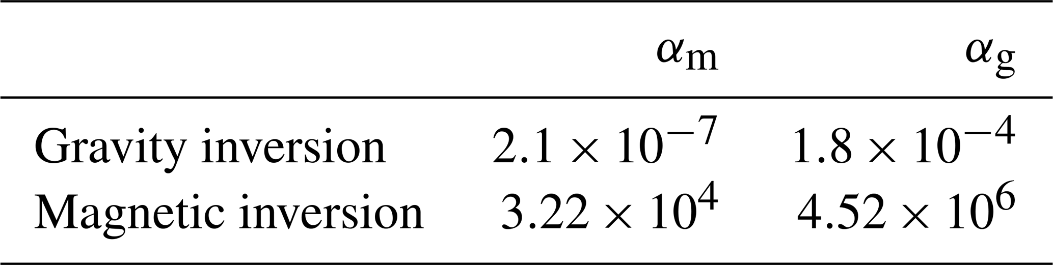
For accurate estimation, the (α_m, α_g) values are sampled more finely closer to the estimated optimum values. The resulting L-surfaces are shown in Fig. 9, where the vicinity of the optimum value of (α_m, α_g) is shown with a green dot. From these values, we estimate the optimum values of (α_m, α_g) reported in Table 1.

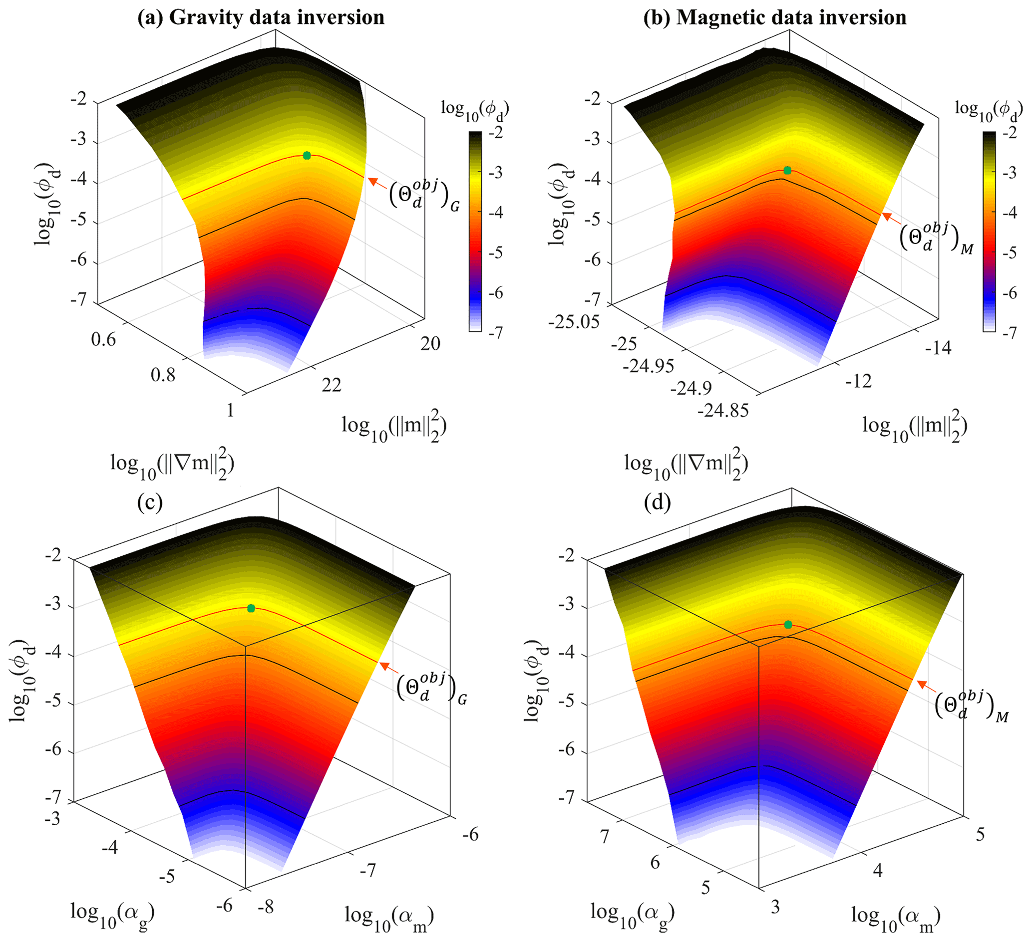
Figure 9 Elbow surfaces for gravity and magnetic inversions (top row) and a plot of the data misfit term as a function of the α weights (bottom row). Each plot uses a total of 1260 points sampling the (α_m,α_g) plane. The black lines show the contour values corresponding to the ticks shown in the palette's colour bar, which shows the value of the data misfit term. The red line materialises the contour value of ${\mathrm{\Theta }}_{\mathrm{d}}^{\text{obj}}$, guiding the selection of the optimum (α_m, α_g) values, and the green dot materialises the vicinity of the curve's inflection point.

Table 1 Optimum values of (α_m, α_g) estimated from L-surface analysis.

The models corresponding to values in Table 1 are shown in Fig. 10.

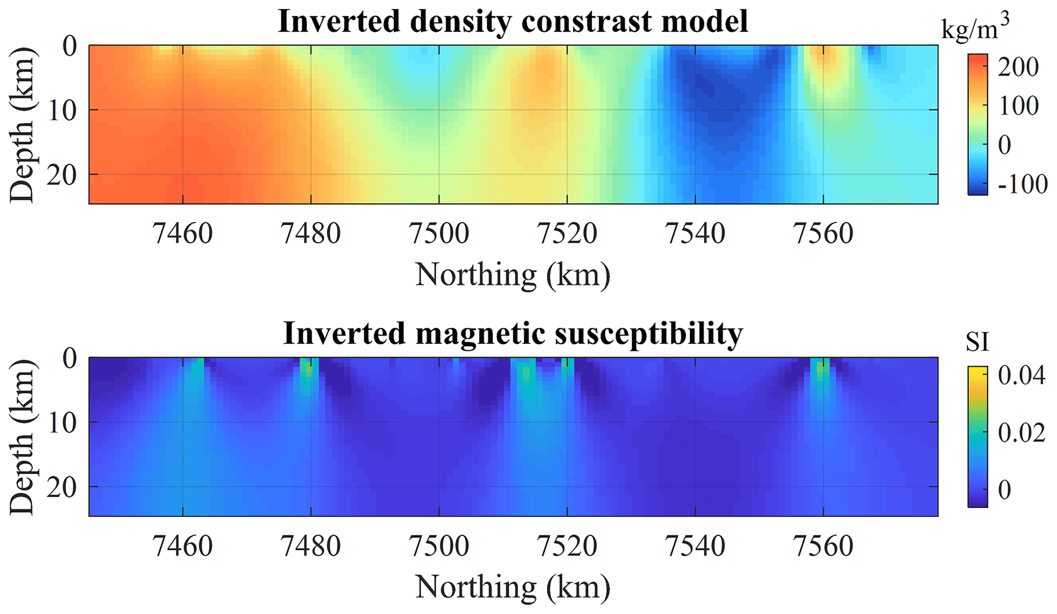
Figure 10 Results from separate inversions using smallness and smoothness constraints. The starting and prior models are equal to zero everywhere, and the smoothness constraint is applied homogeneously.

The values of α_m and α_g obtained for such constraints can be used as a starting point in subsequent inversions to understand the influence of prior information when varying amounts and types of prior information are available about the structure of the subsurface or its petrophysics. For instance, in what follows we will investigate the utilisation of geological information to define W_m and W_g (Eqs. 9 and 10, respectively) and see how it can combined with petrophysical data to define B (Eq. 15) (see the following subsection where we use global and structural and/or petrophysical information). In the case of structural constraints relying on the spatial derivatives of model values (cross-gradient values or local smoothness), the value of α_m may be kept constant and while the other α parameters (α_g or α_x) are adjusted. Conversely, α_g may be kept and α_m set to 0 for the utilisation of petrophysical constraints acting on the model values themselves instead of the spatial derivatives (ADMM or statistical petrophysical constraints). Here, we restrict our analysis to two α values being strictly superior to zero, thereby accounting for prior information in up to two constraints terms in the definition of the regularisation term in Eq. (5).

4.3 Joint inversion using the cross-gradient constraint

We start from the previous step to perform joint inversion using the cross-gradient constraint. Keeping the α_m weight constant and equal to the values determined from single domain inversion, it remains necessary to estimate the optimum values of the cross-gradient constraint weight, α_x, and the relative importance given to the gravity and magnetic data misfit terms (setting α^G=1, it remains to determine α^M). We therefore investigate values in the (α_x,α^M) plane, which we sample in the same fashion as in the previous subsection. The resulting surfaces are shown in Fig. 11.

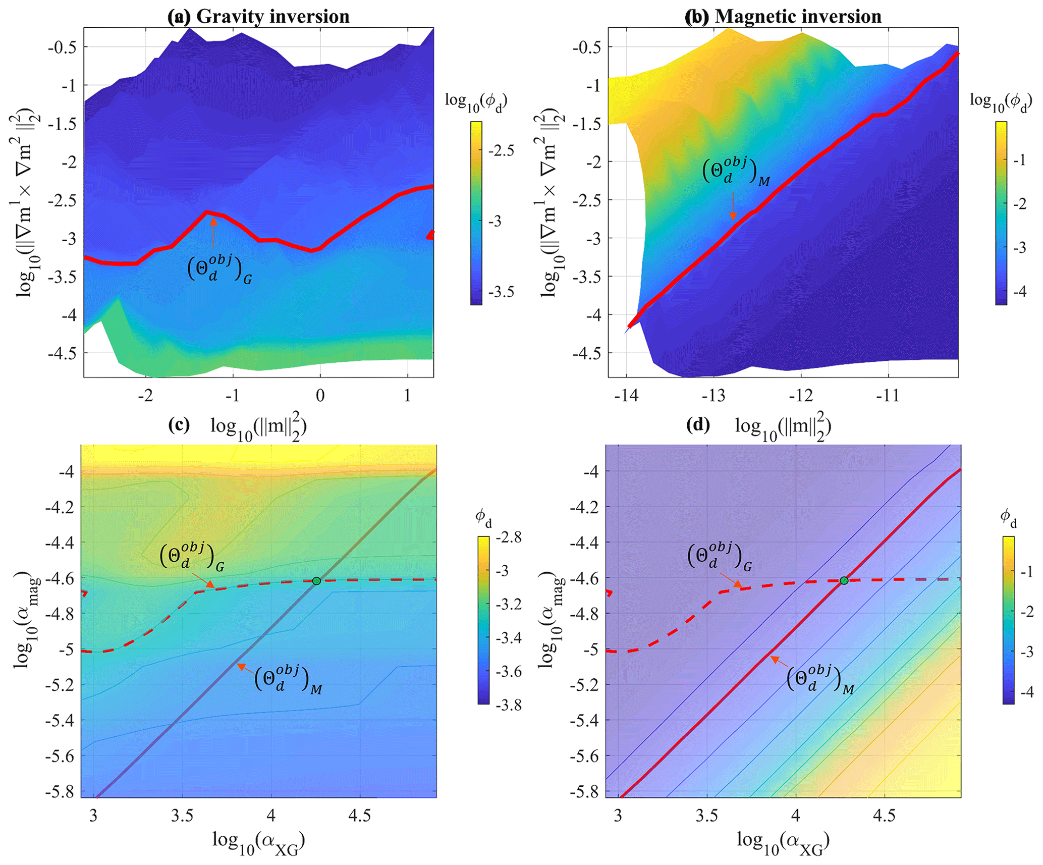
Figure 11 Determination of the optimum (α_x,α^M) parameters in the case of the joint inversion using the cross-gradient constraint. Top view of the elbow surfaces for gravity (a) and magnetic (b) inversions (top row) and a plot of the data misfit term as a function the α weights (bottom row). The solid lines show the contour values of the data misfit; values are given by the colour bar on the side. The solid red line shows the contour level of ${\mathrm{\Theta }}_{\mathrm{d}}^{\text{obj}}$ for the corresponding data set (gravity or magnetic), while the dashed line shows the same quantity for the other data set. The green dot marks their intersection, indicating the optimum (α_x,α^M) values.

In contrast to the single physics inversion shown in Fig. 9, it appears from Fig. 11 that the two hyperparameters to be determined here, α_x and α^M, influence the inversion differently. While the contour levels of the magnetic data misfit show a linear trend in the (α_x,α^M) plane, it is clearly non-linear in the case of gravity data misfit. This difference might be explained by the fact that the cross-gradient is a second-order regularisation (product of two spatial derivatives of model values) linking two models that are otherwise decoupled. In addition, this suggests that in cases differing from this one, the hyperparameter selection may be non-unique. Nevertheless, the value of the optimum value is unambiguous in our case and can be determined easily. From Fig. 11 we obtain $({\mathit{\alpha }}_{\text{x}},{\mathit{\alpha }}_{\text{mag}})=(\mathrm{1.995}\times {\mathrm{10}}^{\mathrm{4}}$, $\mathrm{2.57}\times {\mathrm{10}}^{-\mathrm{5}}$). The corresponding inversion results are shown in Fig. 12.

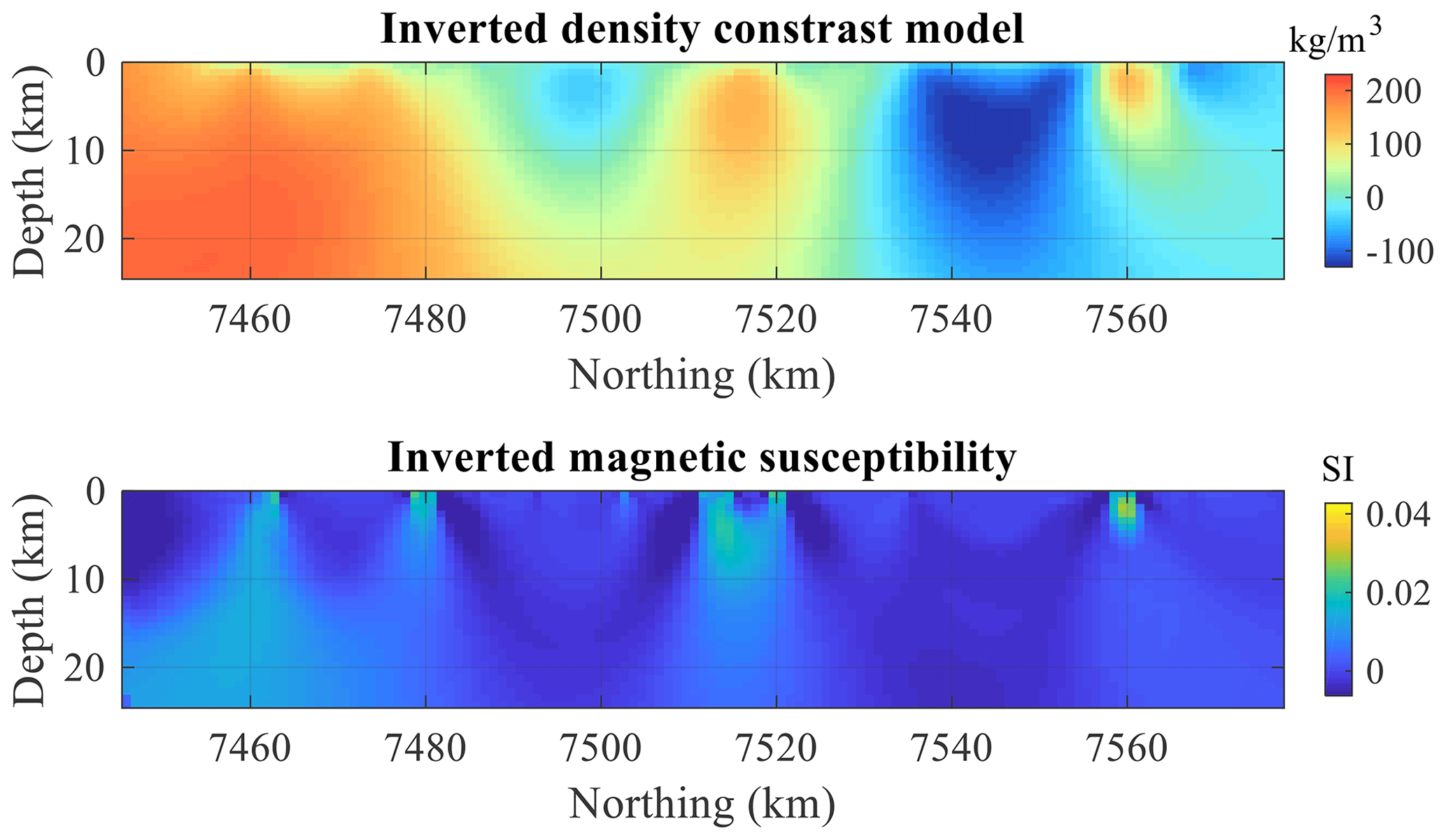
Figure 12 Joint inversion results obtained from utilisation of the cross-gradient constraint.

Compared to Fig. 12, we observe that the application of the cross-gradient constraint leads to adjustments of the model ensuring more structural consistency between density contrast and magnetic susceptibility, illustrating the applicability of the approach presented here. Also note that the model is also visually closer to the true model from approximately 7520 km northing and above. However, despite the increased structural consistency between the density contrast and magnetic susceptibility models, some of the structures of the model are not recovered accurately. For instance, the basin-shape structure around 7500 km northing mirrors the actual geological structure (see Fig. 8) and is an effect of non-uniqueness on inversion. In this case, this illustrates the need for prior information in our inversion. While joint inversion of gravity and magnetic data using the cross-gradient constraint improves imaging comparatively with an inversion constrained only using smallness and smoothness constraints, prior geological information or petrophysical information may be necessary to alleviate the remaining uncertainty.

4.4 Smallness and smoothness constraints using geological information

In this subsection, a sensitivity analysis to prior information in inversion is performed through a series of scenarios where geological structural information is introduced to adjust the smallness and smoothness constraints through W_m and W_g, respectively. In what follows, we apply this approach to gravity inversion.

The influence of geological information in defining the smallness and smoothness terms (detailed in Sects. 2.4.1 and 2.4.2) is analysed by investigating three additional scenarios allowed by the utilisation of either homogenous or geologically derived W_m and W_g matrices. In each case, we start from the (α_m, α_g) weights estimated in Sect. 4.2 from the analysis of the L surface, which we adjust to obtain the geophysical misfit sufficiently close to objective values. We restate that α_m and α_g weight the overall contribution of the model smallness and smoothness, respectively, in the cost function (Eq. 5).

In the first scenario we investigate (scenario b in Table 2), geological uncertainty information is used to define W_m while keeping W_g homogenous. This allows us to test the influence of geological prior information on the smallness term. The values of the diagonal variance matrix W_m are calculated using the geological certainty metric ${\mathit{\sigma }}_{\mathit{\psi }}^{\prime }$ (Eq. 18, shown in Fig. 6b for the 2D section modelled here) and keep W_g homogenous.

Contrary to the previous tests (see Sect. 4.2) where ${\mathbf{W}}_{\mathrm{m}}={\mathbf{I}}_{n_{\mathrm{m}}}$, we find the following result for the kth model cell:

$$\begin{array}{}\text{(20)}& ({\mathbf{W}}_{\mathrm{m}}{)}_{kk}=({\mathit{\sigma }}_{\mathit{\psi }}^{\prime }{)}_k.\end{array}$$

Because $\mathrm{0}\le ({\mathit{\sigma }}_{\mathit{\psi }}^{\prime }{)}_k\le \mathrm{1}\forall k$, we have the following result:

$$\begin{array}{}\text{(21)}& \text{tr}\left({\mathbf{W}}_{\mathrm{m}}\right)=\sum _{i=\mathrm{1}}^{n_{\mathrm{m}}}({\mathit{\sigma }}_{\mathit{\psi }}^{\prime }{)}_i\le \text{tr}({\mathbf{I}}_{n_{\mathrm{m}}})=n_{\mathrm{m}}.\end{array}$$

Consequently, setting W_m in this fashion and keeping α_m constant translates to a lower overall relative importance of the smoothness term in the least-squares cost function (Eq. 5), thereby moving away from the trade-off inferred from the L-curve principle (Sect. 4.2). To mitigate this, we adjust α_m to a value ${\mathit{\alpha }}_{\mathrm{m}}^{\prime }$ such that

$$\begin{array}{}\text{(22)}& {\mathit{\alpha }}_{\mathrm{m}}^{\prime }={\mathit{\alpha }}_{\mathrm{m}}\sqrt{{\displaystyle \frac{n_{\mathrm{m}}}{{\sum }_{i=\mathrm{1}}^{n_{\mathrm{m}}}({\mathit{\sigma }}_{\mathit{\psi }}^{\prime }{)}_i}}},\end{array}$$

which equates $\left({\mathit{\alpha }}_{\mathrm{m}}^{\prime }{)}^{\mathrm{2}}\text{tr}\right({\mathbf{W}}_{\mathrm{m}})$ with (α_m)²n_m so that the overall weight assigned to the smallness term remains the same with and without geological structural information (left-hand side and right-hand side of inequality in Eq. 20, respectively). Because the values of $\Vert {\mathbf{W}}_{\mathrm{m}}\mathit{m}\Vert$ depend on both W_m and m, which vary in space and also depend on the other terms of the cost function, minor adjustments of the value of ${\mathit{\alpha }}_{\mathrm{m}}^{\prime }$ are necessary to reach the objective value of data misfit. In this example, this leads to tune the suggested ${\mathit{\alpha }}_{\mathrm{m}}^{\prime }=\mathrm{8.4}\times {\mathrm{10}}^{-\mathrm{7}}$ to ${\mathit{\alpha }}_{\mathrm{m}}^{\prime }=\mathrm{8.85}\times {\mathrm{10}}^{-\mathrm{7}}$ (keeping α_g constant). The corresponding inverted model is shown in Fig. 13b. The corresponding α weights are repeated in Table 2.

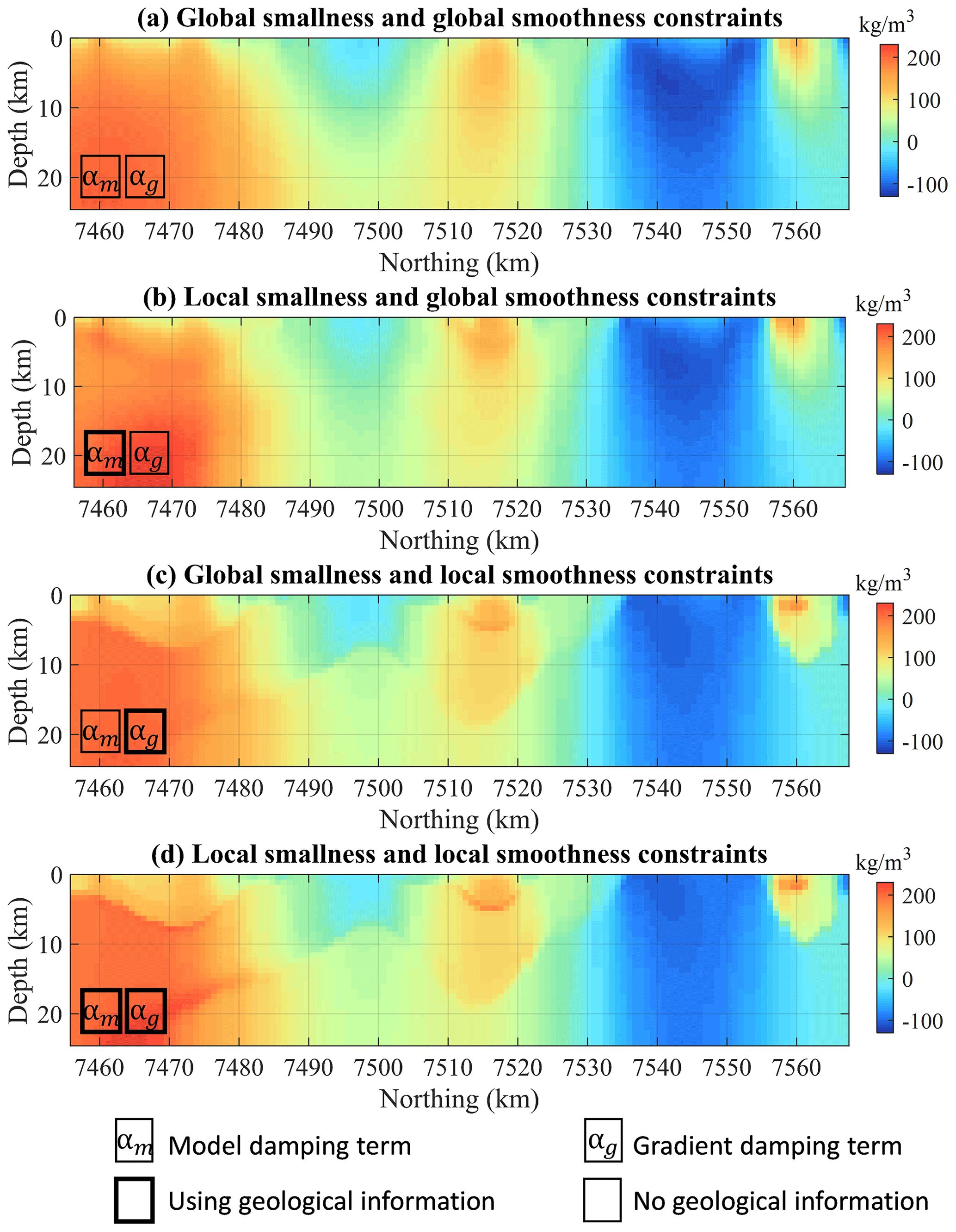
Figure 13 Results from gravity inversion constrained by: (a) homogenous smallness and homogenous smoothness constraints, (b) geologically-derived smallness and homogenous smoothness constraints (c) homogenous smallness and geologically-derived smoothness constraints, (d) geologically-derived smallness and geologically-derived smoothness constraints.

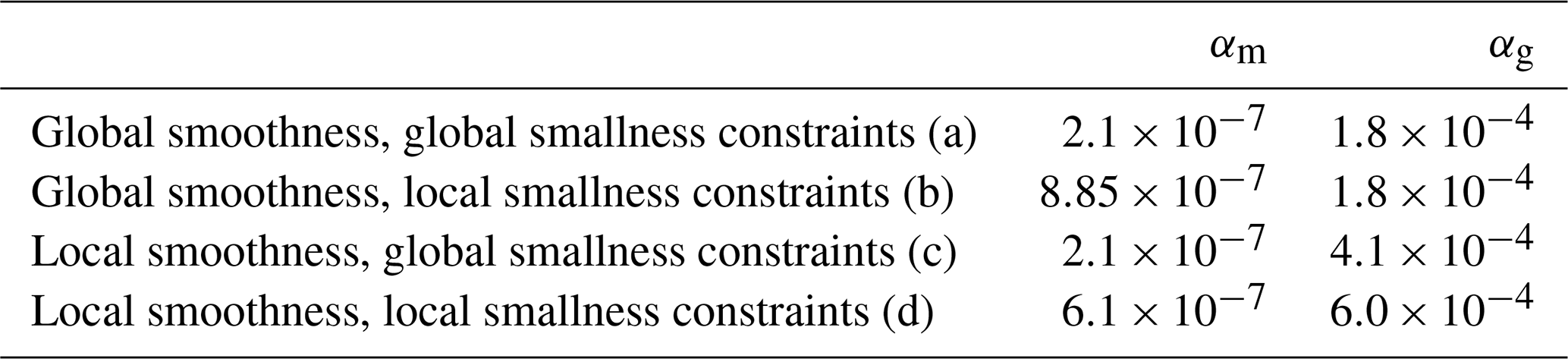
In the second scenario we test (scenario c in Table 2), geological uncertainty information is then used to define W_g while keeping W_m homogenous. This allows us to test the influence of geological prior information on the smoothness term. Following the same procedure as for the smallness term, we adjust the suggested ${\mathit{\alpha }}_{\mathrm{g}}^{\prime }=\mathrm{3.6}\times {\mathrm{10}}^{-\mathrm{4}}$ to ${\mathit{\alpha }}_{\mathrm{g}}^{\prime }=\mathrm{4.1}\times {\mathrm{10}}^{-\mathrm{4}}$. The corresponding inverted model is shown in Fig. 13c. Finally, we test the case where both W_m and W_g are defined using geological information in the form of ${\mathit{\sigma }}_{\mathit{\psi }}^{\prime }$. Starting from values of ${\mathit{\alpha }}_{\mathrm{m}}^{\prime }$ and ${\mathit{\alpha }}_{\mathrm{g}}^{\prime }$ used in the previous tests, minor tuning is performed, leading to ${\mathit{\alpha }}_{\mathrm{m}}^{\prime }=\mathrm{6.1}\times {\mathrm{10}}^{-\mathrm{7}}$ and ${\mathit{\alpha }}_{\mathrm{g}}^{\prime }=\mathrm{6.0}\times {\mathrm{10}}^{-\mathrm{4}}$ inversion results in the model shown in Fig. 13d.

Table 2 The α values derived for simultaneous usage of local and global smallness and smoothness constraints. Scenario (a) is a reminder of the values obtained in Sect. 4.2 when only global constraints are used.

As can be seen in Fig. 13 by comparing Fig. 13a–b with Fig. 13c–d, the utilisation of geological structural information to adjust the smoothness regularisation strength spatially has more impact on inversion than adjusting the smallness term. While incorporating prior geological information in W_m constrains the model to a certain extent, using C_v to derive W_g has more influence on the inverted model than for W_m, with resulting models that are closer to the reference model.

Comparing Fig. 13c and d indicates that the use of geological uncertainty information to adjust the smallness regularisation strength spatially (through W_m) in addition to the model smoothness term (through W_g) modifies inversion results further towards the reference model. Figure 13d, which results from inversion using prior information in both constraint terms, provides the model closest to the reference. While most interfaces are well-recovered when using geological information to define both W_g and W_m, the recovered density contrasts remain affected by the ambiguity inherent to gravity data in the presence of subhorizontal geological units (around 7460 km northing). This suggests that in this example, more prior information might be useful in recovering the causative model more truthfully, especially in cases where potential field inversion is ambiguous (e.g. subhorizontal interfaces for gravity inversion). This is the object of the next subsection, which describes a new single physics inversion scenario where petrophysical constraints are combined with structural constraints and geological information.

4.5 Structural and petrophysical constraints

In addition to the definition of matrices W_m and W_g, geological information can be combined with petrophysical knowledge to define the range of density values allowed in inversion. This is achieved with spatially varying bound constraints on the property inverted for density contrast in this case (see Sect. 2.4.5). Here, such bounds are defined using multiple intervals, each one corresponding to the range of density contrast values expected for a geological unit. Such bounds can be defined globally (homogenously) where all intervals are allowed everywhere in the model or locally when prior information about the presence of the rock units is available. In this work, we use the probability of occurrence of the different rock units to derive bounds that vary in space accordingly with the probability of observation of each of the rock units. In a given cell, only the bound values corresponding to rock units with a probability Ψ>0 are considered. Starting from Eq. (15), such spatially varying bounds B_k of the kth model cell are obtained as follows:

$$\begin{array}{}\text{(23)}& B_k=\underset{{\mathrm{\Psi }}_{k,l}>\mathrm{0}}{\bigcup _{l=\mathrm{1}}^{n_{\mathrm{f}}}}[a_{k,l},b_{k,l}],\end{array}$$

where a and b correspond to lower and upper bounds. We consider narrow bounds such that $b_{k,l}=a_{k,l}+\mathit{\epsilon }$, with $\mathit{\epsilon }\ll a_{k,l}$, to encourage inversion to use density contrasts that closely resemble values defined a priori. Equation (23) corresponds to the application of a Boolean operator to the probabilities ${\mathrm{\Psi }}_{k=\mathrm{1}\mathrm{\dots }{n}_{\mathrm{f}}}$ in every cell to divide the studied area into domains defined by rock units with a probability Ψ>Ψ_th. In such cases, the ADMM bound constraints act as a proxy for a prior models that have been dynamically constrained by petrophysical information.

Four additional scenarios are tested to determine the influence of prior information on inversion to accommodate the addition of both the damping gradient and ADMM bound constraint term. The use of prior information is illustrated in Fig. 14.

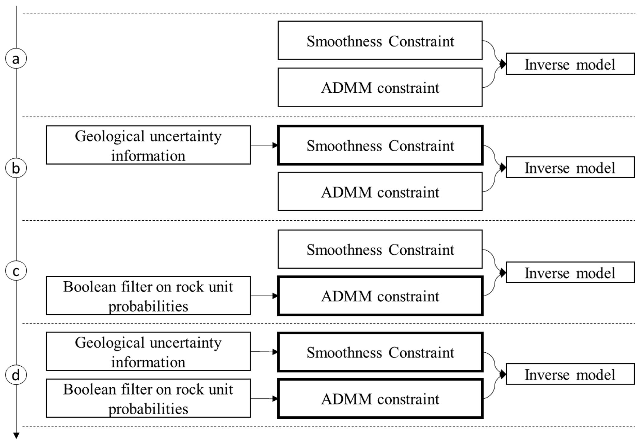
Figure 14 Tested combinations for the utilisation of prior information into inversion. Bold frames indicate the utilisation of geological information to define the constraints.

At a given iteration, the ADMM bound constraint encourages inverted values to evolve inside one of the prescribed intervals depending on the current model m. As mentioned above, we can then make the analogy with a smallness term that is dynamically updated. For this reason, we treat the ADMM bound constraints in the same fashion as the smallness term, which we apply simultaneously to the model smoothness term.

Following the same protocol as Sect. 4.1 to determine α_g and α_a, we first perform inversion without the use of geological information in the form of the probabilities for the occurrence of different rock units or metrics that can be derived from them (Fig. 14a, i.e. with W_g and W_a equal to the identity matrix and the corresponding regularisation term weighted by α_g and α_a, respectively). It is therefore necessary to determine the value of α_g and α_a (Eq. 5). We perform an L-surface analysis and sample values in the (α_g,α_a) plane to estimate the optimum values for these hyperparameters (see Fig. 15). Values of α_g vary from $\mathrm{1.585}\times {\mathrm{10}}^{-\mathrm{7}}$ and $\mathrm{1.585}\times {\mathrm{10}}^{-\mathrm{5}}$, and values of α_a vary from $\mathrm{2.484}\times {\mathrm{10}}^{-\mathrm{5}}$ and $\mathrm{2.484}\times {\mathrm{10}}^{-\mathrm{7}}$. The resulting L-surface is shown in Fig. 15.

Figure 15 Elbow surfaces for gravity inversions. A total of 840 points sampling the (α_g,α_a) plane were used. The black lines show the contour values corresponding to the ticks shown in the palette's colour bar, which shows the value of the data misfit term. The red line indicates the contour value of ${\mathrm{\Theta }}_{\mathrm{d}}^{\text{obj}}=\mathrm{5.008}\times {\mathrm{10}}^{-\mathrm{4}}$, guiding the selection of the optimum (α_g,α_g) values, and the green point indicates the curve inflection point.

From Fig. 15, we estimate the hyper-parameters (α_g,α_a) to be $({\mathit{\alpha }}_{\mathrm{g}},{\mathit{\alpha }}_{\mathrm{a}})=(\mathrm{2.2}\times {\mathrm{10}}^{-\mathrm{5}},\mathrm{1.3}\times {\mathrm{10}}^{-\mathrm{7}})$ in the case no geological information is used, meaning that both constraints are applied homogenously across the model.

From there, we follow the same procedure as described above (Sect. 4.1 and 4.2) to obtain an estimate for the values of α_a and α_g in the different configurations shown in Fig. 14b–d. The resulting inverted models are shown in Fig. 16, and the estimates of (α_g,α_a) are provided in Table 3.

Table 3 The α values derived for simultaneous usage of global and local smoothness and ADMM bound constraints. Cases (a) through (d) correspond to cases (a) through (d) in Fig. 14.

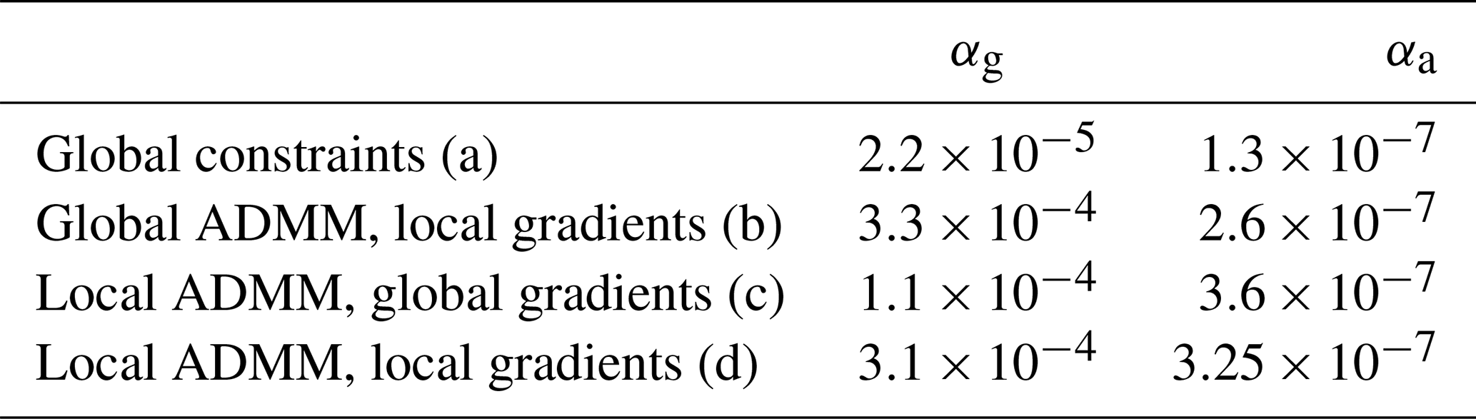
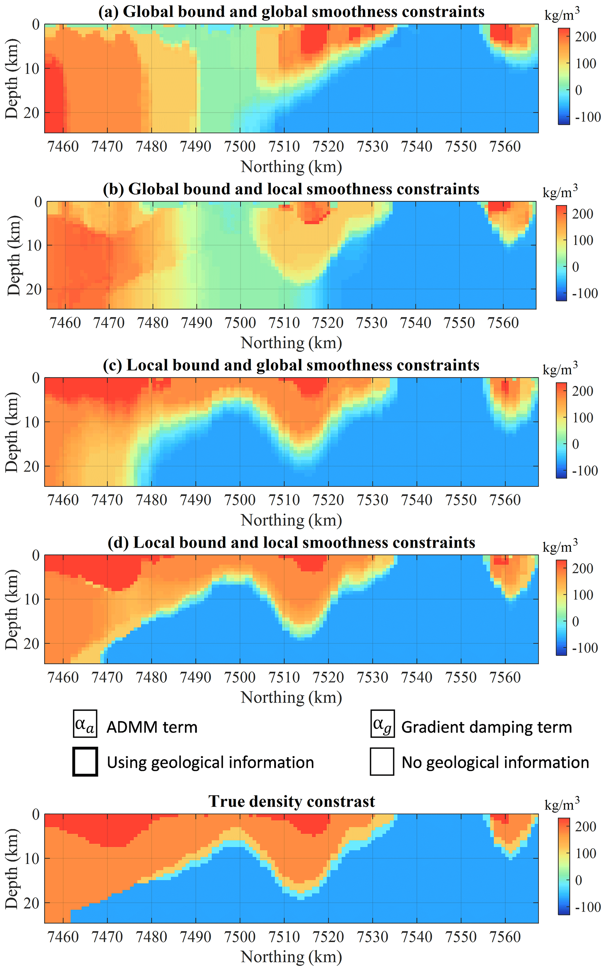
Figure 16 Results from gravity inversion using (a) global ADMM clustering and homogenous smoothness constraints, (b) global ADMM clustering and geologically derived smoothness constraints, (c) ADMM clustering and geologically derived smoothness constraints, and (d) geologically derived ADMM clustering and geologically derived smoothness constraints. For visual comparison, the true model is repeated at the bottom.

Figure 16 shows that the use of ADMM facilitates recovery of better-defined interfaces between rock units than in previous inversions (Figs. 10, 12, and 13), and decreases the misfit with the causative model (shown in Fig. 6). Unsurprisingly, without the use of geological information (Fig. 16a) inversion results remain inconsistent with geology in several parts of the model, especially around the position 7500 km northing. The inconsistent results can be partly mitigated by using geologically derived smoothness constraints (Fig. 16b). In comparison, however, Fig. 16c shows that use of geological information to determine the bounds recovers features much closer to the causative model.

While Fig. 16d shows the more robust results overall, Fig. 16c and d present generally similar features. This indicates that in this case geological uncertainty information in structural constraints only allows the refining of features largely controlled by the utilisation of the ADMM constraints. This statement is supported by Fig. 16, where the comparison cases (a and b) and (c and d) reveal that the effect of using geological information to define bounds dominates over the effect of using uncertainty to define structural constraints.

The comparison of cases (a and b) and (c and d) in Fig. 16 can be extrapolated to Figs. 13 and 16 to compare constraints more broadly. This is discussed in Sect. 5.1, which presents a short comparative analysis of all gravity inversion results.

5 Discussion

5.1 Sensitivity analysis summary: comparison of constrained inversions

Tomofast-x was developed with the intent of providing practitioners with an inversion platform accounting for various forms of prior information and geophysical data sets. We have tested a series of constraints involving joint inversion and geological and petrophysical information. The inverted density contrast models for inversion using global smallness and smoothness constraints, joint inversion using the cross-gradient technique, geologically derived smallness and smoothness constraints, and ADMM bound constraints (both global and using geological information) are shown in Fig. 17. We remind that all models shown here produce a similar data misfit ${\mathrm{\Theta }}_{\mathrm{d}}^{\text{obj}}$ accordingly with Eq. (19).

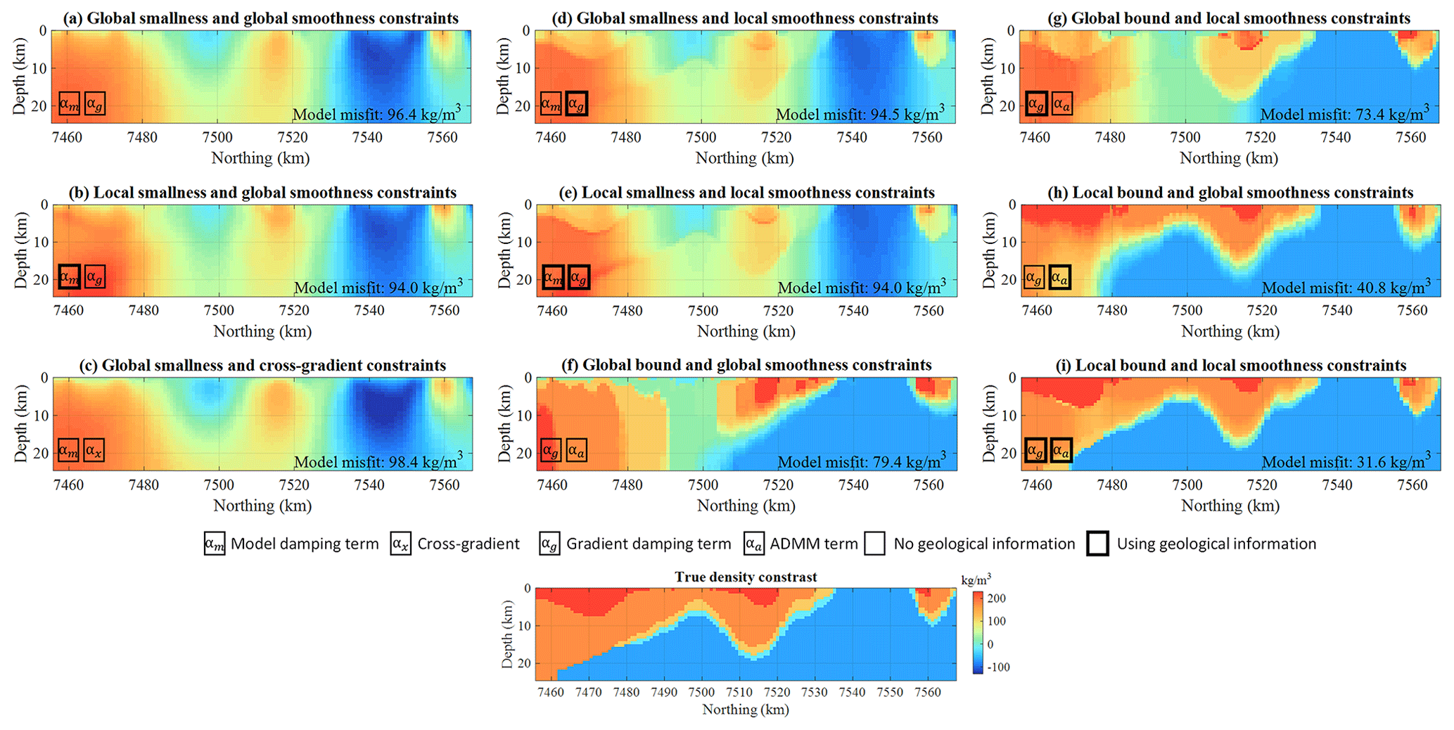
Figure 17 General comparison of all inversion results obtained from gravity inversion. The legend identifies the different types of inversion shown. We repeat the true model at the bottom. The model misfit indicated on each panel is calculated as the root mean square of the difference between the inverted and true models.

Firstly, it appears from Fig. 17 that regardless of the type of constraints considered, the utilisation of geological information (cases b, d, e, g–i) to derive spatially varying constraints for the W matrix of both terms used provides the models that are visually closest to the true model. In this category, the utilisation of petrophysical information in the ADMM bound constraints provides (cases h–i) models that are closest to the true model (the lowest model misfit values are indicated in the titles of the panels in Fig. 17). Secondly, the comparison of cases (a) and (d), (b) and (e), (f) and (g), and (h) and (i) indicates that while it has a less significant influence on the results, incorporating geological information in the definition of the smoothness term also influences inversion results significantly. Lastly, comparison of cases (a) and (b) and (d) and (e) suggests that the utilisation of geological information to adjust the smallness strength spatially has an effect on inversion that is the lowest with the cross-gradient constraints (where structural information is passed on from another geophysical data set).

From the results shown in Sect. 4.2 through 4.5 and compared in Fig. 17, it is possible to make a qualitative ranking of the constraints according to their influence on the resulting model (from the most important influence to the least important influence): ADMM bound constraints > smoothness constraints > smallness constraints > cross-gradient constraints. This observation is also corroborated by the values of the root-mean-square misfit between the true and inverted model. We note that this ranking remains speculative as it might apply only to models sharing similarities with the case we investigated.

From these observations we also deduce that when geological uncertainty information is added to the definition of constraints (i.e. ${\mathit{\sigma }}_{\mathit{\psi }}^{\prime }$ for defining W_m and W_g and probabilities for defining B), the term of the cost function with the highest influence on the process will determine the main features of the model, which will be adjusted by the other term.

Tomofast-x was developed with the intent of providing practitioners with an inversion platform allowing various forms of prior information and geophysical data. Constraints that represent uncertainty and our level of epistemic knowledge provide useful constraint to inversion. This is encouraging as the Tomofast-x platform addresses a gap in inversion schemes that rely on a single model, with the model being as similar as possible to the target region, an often impossible requirement to meet. Thus, Tomofast-x opens additional research avenues to the community that are widely acknowledged but remain largely unaddressed. Conceptual uncertainty relating the prior assumptions made about tectonic event history of the region, and thus the structure under study, can be analysed. Different event histories and topologies can be considered, giving a wider scope to the model space, and allowing the geophysics to invalidate implausible histories, while giving us pause to consider other histories that may be less likely but that are nonetheless possible.

5.2 Outlook for future developments

Another research avenue under consideration is the integration of results from probabilistic modelling of seismic and electrical data into Tomofast-x. As stated in the introduction, one of the goals born in mind during the design of Tomofast-x is interoperability. Current work involves the integration of Tomofast-x into the Loop¹ open-source 3D probabilistic geological and geophysical modelling platform (Ailleres et al., 2019), in an effort to unify geological and geophysical modelling at a more fundamental level than the more common cooperative approaches. Ongoing developments include the possibility to adjust weight assigned to the ADMM bound constraints accordingly with uncertainty levels in prior information used to define spatially varying intervals.

Future research includes the utilisation of implicit geological modelling (in the sense of Calcagno et al., 2008) with Tomofast-x to define geological structures and rules that inversion will be encouraged to follow. It also comprises the incorporation of topological laws previously used a posteriori (Giraud et al., 2020) directly into inversion. The electrical capacitance tomography component of Tomofast-x (Martin et al., 2018), which we have not detailed here, can be extended to acoustic (seismic) or electromagnetic data inversions that rely on the resolution of similar non-linear inversion problems. It opens the door to more versatility in the code and can be applied to joint inversion in similar ways but on more than two physical domains.

In addition, future developments comprise the collaborative and joint inversion of seismic and potential field data. It is planned to develop an interface between Tomofast-x and Unisolver (not yet released as open source by its authors), which is an extension of Seimic_Cpml code (Komatitsch and Martin, 2007; Martin et al., 2010, 2019), where integrated seismic imaging solvers are implemented. Unisolver is a multi-purpose 2D and 3D seismic imaging platform based on high-order finite-difference and finite-volume discretisation and non-linear seismic data inversion procedures. Such an interface would allow performing collaborative or joint inversion of seismic and gravity or magnetic data and could obtain the resulting models on the same mesh while benefitting from Tomofast-x's various functionalities. This will be an easy way to provide Tomofast-x with separate seismic information on the fly like sensitivity kernels as another physical domain.

In the implementation presented here, only the truncation of the matrix system based on maximum distance thresholding was discussed. It is planned to reduce memory requirements using the wavelet compression of the matrix system of the inverse problem in the same fashion as Martin et al. (2013).

We have shown a number of tests using a selected set of functionalities of Tomofast-x. However, more or different tests could be done. For instance, an interesting research avenue is to exploit Tomofast-x's capability to read an arbitrary number of prior and starting models to test the geological archetypes that can be identified by clustering of the set of geological models probabilistic geological modelling can produce (Pakyuz-Charrier et al., 2019). Additional features of Tomofast-x, the testing of which lies beyond the scope of this paper, are Jacobian matrix truncating and different kinds of depth weighting and their effects on the different types of inversion. Finally, we have not used posterior uncertainty indicators listed in Sects. 2.5 and A1 as the paper focusses on the inversion capabilities of Tomofast. However, the output results of Tomofast-x allow us to study uncertainty in the same fashion as Giraud et al. (2017, 2019c) where some of them are used.

Results obtained using the cross-gradient technique for joint inversion of gravity and magnetic data showed that it can improve imaging of geological structures. However, our study also revealed some of the limitations of this method. In the synthetic example, structurally coherent features of the resulting model contradict the geology of the true model. In addition, our L-curve (or L-surface) analysis suggests that the determination of the optimum α weights of the cost function using the cross-gradient technique may be affected by non-uniqueness and that multiple sets of weights could equally satisfy the L-curve criterion. One interpretation is that this method remains affected by uncertainty and could be producing several families of models fitting geophysical data equally well. This observation differs from similar analysis performed in the case of joint inversion using petrophysical constraints, where such potential ambiguity was not suggested by the L-surfaces (Giraud et al., 2019c). These impressions, however, require a more detailed investigation and constitute a new research avenue.

In our sensitivity analysis, we have produced a series of models that can be considered geophysically equivalent because they fit the geophysical data equally well. These models are the result of deterministic inversion, where prior information guides inversion towards one of the modes of the probability density function describing the problem (Eq. 1) or modifies them. It is therefore safe to assume that each mode is representative of an archetype of models from the geophysical data's null space. This highlights the interest of using “null-space shuttles”, allowing navigation of the null space (Deal and Nolet, 1996; Muñoz and Rath, 2006; Vasco, 2007; Fichtner and Zunino, 2019) to explore the space of possible models without extensive sampling and to assess the robustness of the result. In addition, the plots of the L-curves corresponding to the problem we presented suggest the presence of multiple optima in the hyperparameter space (weights α), which it might be interesting to investigate in future research, especially in the joint inversion case.

6 Conclusions

We have introduced the open-source joint inversion platform Tomofast-x and demonstrated its capabilities with a realistic data set taken from the Hamersley region in central Western Australia. The geophysical theoretical background of Tomofast-x was explained in depth to guide users in understanding and using the modelling approach implemented in the source code.

We leveraged the modularity of Tomofast-x to study the sensitivity of inversion to prior structural, geological, and petrophysical information; joint inversion; and the code's scalability. We tested a new combination of constraints incorporating geological structural information in the smoothness term and dynamic prior model definition using petrophysical knowledge (ADMM bound constraints), a feature usually not available to most inversion software. Our sensitivity analyses on prior information and different constraints reveal that constraints using petrophysics (ADMM bound constraints) dominate over gradient-based constraints (smoothness and cross-gradient constraints), which in turn exert more influence on inversion than smallness constraints. This shows the importance of prior information in inversion and illustrates the need to study the space of geophysically equivalent models.

The examples described here were designed to replicate a typical, rigorous approach to the development of a geoscientific model and be relevant to real-world application. The aim to ensure rigour and reproducibility of the result presented is facilitated by the release of the source code, data sets, and a reduced modified Python version of the algorithm that accompany this paper.

Appendix A: Other functionalities of Tomofast-x

A1 Posterior uncertainty indicators

A1.1 Posterior LSQR variance matrix

At the first and last iteration of the inversion, the diagonal elements of the posterior covariance matrix of the recovered model are calculated in Tomofast-x (see Sect. 2.5). The variances are part of the outputs of Tomofast-x for further analysis by the user, such as the estimation of uncertainty in the recovered property model.

A1.2 Jacobian of the cost function

Tomofast-x offers the possibility to examine the Jacobian matrix of the cost function (Eq. 5), which encapsulates the contribution of several constraint terms (see for example Eq. 5), by calculating its derivative with respect to the model m, $\partial \mathit{\theta }(d,m)/\partial m$. This feature takes advantage of the LSQR solver. In the LSQR algorithm, $\partial \mathit{\theta }(d,m)/\partial m$ is calculated at the beginning of each iteration when approximating a solution to the system of equations (Appendix E). The value of $\partial \mathit{\theta }(d,m)/\partial m$ can then be calculated before or after application of the depth-weighting operator. It is computed as the product of the transpose of the matrix representing the left-hand side of the system of equations to be solved by the vector of the corresponding quantities to minimise data misfit, cross-gradients, damping terms, etc. (constituting the right-hand side of the corresponding equation, as shown in Appendix E). Importantly, its dimension is equal to the number of model parameters. It is therefore possible to store it on disk to provide a measure of the sensitivity of the data and the different terms of the misfit function to model variations at depth or in any part of the computational domain. By computing $\Vert \partial \mathit{\theta }(d,m)/\partial m\Vert$, it is possible to study the convergence of the algorithm, with small values indicating convergence. In addition, it is a metric that measures the stability of the algorithm and which is useful to determine whether the system of equations is well conditioned.

A1.3 Identification of rock units

Membership analysis of the inverted model can be performed when statistical petrophysical constraints were applied to inversion from the values of 𝒩_k reached after inversion converged. Membership values can be used to assess inverted models by reconstructing a rock unit model from the recovered inverted physical properties (Doetsch et al., 2010; Sun et al., 2012; Giraud et al., 2019c). Rock units labels can also be assigned to model cells when the ADMM bound constraints have converged. It allows attaching a petrophysical property interval to each model cell, allowing direct identification of rock types.

A1.4 Cross-product of gradients

The cross-product of model gradients in 3D can be stored after inversion and its L₂ norm is given after each inversion cycle. It allows us to assess the degree of structural similarity between the models and to delineate areas showing specific structural similarities or dissimilarities.

A2 Jacobian matrix truncation

Tomofast-x offers the possibility to use a moving sensitivity domain approach (Čuma et al., 2012; Čuma and Zhdanov 2014), limiting the sensitivity domain to a cylinder, the radius of which is chosen by the user, to reduce computational requirements (the option for a sphere is also present in the source code but commented in the current version). The underlying assumption is that cells beyond a given distance exert a negligible influence on the measurement. Generally speaking, this radius is provided by the users and should be chosen carefully.

A3 L_p norm

Tomofast-x also offers the possibility of performing data inversion using a L_p norm ($\mathrm{1}<p\le \mathrm{2}$) to define the smallness term, as it has been proposed for electrical capacitance tomography (ECT) in Martin et al. (2018) in the framework of Tomofast-x. The L_p norm inverse problem is non-linear and can be solved iteratively using L₂ minimisation. In the L_p norm case, the regularisation parameter can be approximated by a p-power law of the model at each point of the computational domain and must also be recomputed at each new inversion cycle. When the L_p norm is introduced for p<2, this procedure allows us to obtain sharper models with better interface definition and determine stronger contrasts for the specific cases under study. If p=2, the smallness term is reduced to L₂ norm minimisation (the commonly used Tykhonov-like regularisation) as used in this work. The choice of other values such that $\mathrm{1}<p\le \mathrm{2}$ is at the discretion of the user or depending on prior information.

A4 Electrical capacitance tomography

Detailing electrical capacitance tomography (ECT) is beyond the scope of this paper, but we can apply to joint gravity and magnetic inversion the functionalities that have been introduced to solve the ECT inverse problem based on L₂ data misfit norm and L_p ($\mathrm{1}<p\le \mathrm{2}$) damping term minimisation (see Sect. A3). In Tomofast-x, ECT is based on the finite-volume method for the forward problem and on a non-linear and iterative LSQR method to solve the inverse problem. As in propagative and diffusive geophysical inverse problems in frequency domain, the sensitivity matrix and the damping term depend on the current model and must be recomputed at each new iteration. We refer the reader to Martin et al. (2018) for more details on this technique. Note that algorithms developed in relation to this method can easily be extended to propagative and diffusive geophysical inverse problems.

Appendix B: Summary of the notation and terms used in the paper

Symbol	Definition
Subscripts and superscripts
d	refers to “data”, i.e. “mag” or “grav”
m	model
pr	refers to “prior”
g	gradient
x	cross-gradient
pe	refers to “petrophysics”
a	ADMM
G	gravity
M	magnetics
Model and physical quantities
m	property model inverted for
z	ADMM variable
u	ADMM variable
ω	membership value in Gaussian mixture
ψ	membership value in Gaussian mixture (from geology)
μ	mean value of petrophysical properties
σ	standard deviation of petrophysical properties
ε	positive threshold real number such that z≫ε
ndata	number of geophysical data points
nf	number of rock formations
d	geophysical data
β	exponent for depth-weighted power law
Mathematical operators or notations
g(.)	geophysical forward operator
P(⋅)	petrophysical distribution operator
∇⋅	gradient operator
Lp	Lp norm
L2	L2 norm (sum-of-squares)
S	geophysical data sensitivity matrix
diagonal matrices W
Wd	diagonal matrix where all elements are equal to the inverse of the sum of squares of the data
Wm	smallness term covariance matrix
Wg	smoothness term covariance matrix
Wx	cross-gradient term covariance matrix
Wpe	petrophysical term covariance matrix
Wa	ADMM term covariance matrix
D	depth-weighting operator
weighting terms α
αm	model
αg	gradient
αx	cross-gradient
αpe	petrophysics
αa	multiple bound constraints
αG	weight assigned to the gravity inverse problem (used only in joint inversion)
αM	weight assigned to the magnetic inverse problem (used only in joint inversion)

Appendix C: Forward gravity and magnetic data calculation

In this Appendix we summarise the forward calculation of gravity and magnetic data as performed in Tomofast-x. In practice, Tomofast-x calculates forward data using input data expressed in units from Système International (SI), expressed in kilograms, metres, and seconds. The gravity field f of a distribution of density anomalies Δρ over a volume of rock V at a location ${\mathit{r}}^{\prime }=[x^{\prime },y^{\prime },z^{\prime }]$ can be expressed as follows:

$$\begin{array}{}\text{(C1)}& f\left(\mathit{r}\right)=G\underset{V}{\iiint }\mathrm{\Delta }\mathit{\rho }\left(\mathit{r}\right){\displaystyle \frac{\mathit{r}-{\mathit{r}}^{\prime }}{|\mathit{r}-{\mathit{r}}^{\prime }{|}^{\mathrm{3}}}}\mathrm{d}V,\end{array}$$

where $\mathit{r}=[x,y,z]$ defines the location of mass density anomaly Δρ(r) and G is the universal gravity constant. While Tomofast-x is implemented in such a way that the three spatial components of f can be obtained, we consider only the vertical direction here, which we simply write as f for sake of clarity (note that here, when taken for the whole model, f=g_G). In our implementation, the volume V is discretised in N_m rectangular prisms (model cells) of constant density. Discretised, Eq. (C3) then rewrites as follows:

$$\begin{array}{ll}{\displaystyle }f(x,y,z)=& {\displaystyle }G{\sum }_{k=\mathrm{1}}^{N_{\mathrm{m}}}\mathrm{\Delta }{\mathit{\rho }}_k\\ {\displaystyle }& {\displaystyle }\times {\displaystyle \frac{z_k-z^{\prime }}{\left(\right(x-x_k{)}^{\mathrm{2}}+(y-y_k{)}^{\mathrm{2}}+(z-z_k{)}^{\mathrm{2}}{)}^{\frac{\mathrm{3}}{\mathrm{2}}}}}\\ \text{(C2)}& {\displaystyle }& {\displaystyle }\times \mathrm{\Delta }{x}_k\mathrm{\Delta }{y}_k\mathrm{\Delta }{z}_k,\end{array}$$

where Δx_k, Δy_k, and Δz_k define the dimensions of the kth rectangular prism. In our discretisation, we assume a model constituted of $n_x\times n_y\times n_z$ cells, with n_x, n_y, and n_z representing the number of cells in each direction. This leads to the computation of f using the following formulation of Eq. (C1):

$$\begin{array}{}\text{(C3)}& f(x,y,z)=\sum _{i=\mathrm{1}}^{n_x}\sum _{j=\mathrm{1}}^{n_y}\sum _{k=\mathrm{1}}^{n_z}\mathrm{\Delta }{\mathit{\rho }}_{i,j,k}{\mathbf{S}}_{i,j,k},\end{array}$$

where, using the formulation of Blakely (1995), the elements of the sensitivity matrix S are given as follows:

$$\begin{array}{ll}{\displaystyle }{\mathbf{S}}_{i,j,k}=& {\displaystyle }G\sum _{m=\mathrm{1}}^{\mathrm{2}}\sum _{q=\mathrm{1}}^{\mathrm{2}}\sum _{t=\mathrm{1}}^{\mathrm{2}}(-\mathrm{1}{)}^{m+q+t}\\ {\displaystyle }& {\displaystyle }\times \left[{\mathit{\zeta }}_t\text{atan}\right({\displaystyle \frac{{\mathit{\xi }}_m{\mathit{\eta }}_q}{{\mathit{\zeta }}_t{R}_{m,q,t}}})\\ \text{(C4)}& {\displaystyle }& {\displaystyle }-{\mathit{\xi }}_m\log (R_{m,q,t}+{\mathit{\eta }}_q)-{\mathit{\eta }}_q\log (R_{m,q,t}+{\mathit{\xi }}_m)],\end{array}$$

where ξ_m, η_q, and ζ_t are the coordinates of the vertices of the prism and

$$\begin{array}{}\text{(C5)}& R_{m,q,t}=\left[\right(x-{\mathit{\xi }}_m{)}^{\mathrm{2}}+(y-{\mathit{\eta }}_q{)}^{\mathrm{2}}+(z-{\mathit{\zeta }}_t{)}^{\mathrm{2}}{]}^{\frac{\mathrm{1}}{\mathrm{2}}}.\end{array}$$

In Tomofast-x, the total magnetic field anomaly is calculated by summing the responses of the prisms making up the model, following Bhattacharyya (1964, 1980). The regional magnetic field is denoted $\mathit{F}=(F_x,F_y,F_z)$, and the magnetisation is denoted $\mathit{M}=(M_x,M_y,M_z)$. We write $F=\Vert \mathit{F}\Vert$ and $M=\Vert \mathit{M}\Vert$. Note that remnant magnetisation is not accounted for.

Using the formalism of Blakely (1995), we denote ΔT the magnitude of the total magnetic field anomaly generated by a prism oriented parallel to the x, y, and z axes of the mesh similarly to the gravity case. We have the following equation:

$$\begin{array}{}\text{(C6)}& \mathrm{\Delta }T(x,y,z)=\sum _{i=\mathrm{1}}^{n_x}\sum _{j=\mathrm{1}}^{n_y}\sum _{k=\mathrm{1}}^{n_z}{\mathit{\chi }}_{i,j,k}{\mathbf{S}}_{i,j,k},\end{array}$$

where χ is the magnetic susceptibility. The sensitivity S is given as follows:

$$\begin{array}{ll}{\displaystyle }{\mathbf{S}}_{i,j,k}=& {\displaystyle }{\mathit{\mu }}_{\mathrm{0}}F\sum _{m=\mathrm{1}}^{\mathrm{2}}\sum _{q=\mathrm{1}}^{\mathrm{2}}\sum _{t=\mathrm{1}}^{\mathrm{2}}(-\mathrm{1}{)}^{t+\mathrm{1}}\\ {\displaystyle }& {\displaystyle }\times \left[{\displaystyle \frac{{\mathit{\alpha }}_{yz}}{\mathrm{2}}}\log \right({\displaystyle \frac{R_{m,q,t}-{\mathit{\xi }}_m}{R_{m,q,t}+{\mathit{\xi }}_m}})\\ {\displaystyle }& {\displaystyle }+{\displaystyle \frac{{\mathit{\alpha }}_{xz}}{\mathrm{2}}}\log \left({\displaystyle \frac{R_{m,q,t}-{\mathit{\eta }}_q}{R_{m,q,t}+{\mathit{\eta }}_{q_m}}}\right)\\ {\displaystyle }& {\displaystyle }-{\mathit{\alpha }}_{xy}\log (R_{m,q,t}+{\mathit{\zeta }}_t)\\ {\displaystyle }& {\displaystyle }-M_x{F}_x\text{atan}\left({\displaystyle \frac{{\mathit{\xi }}_m{\mathit{\eta }}_q}{{\mathit{\xi }}_m^{\mathrm{2}}+R_{m,q,t}{\mathit{\zeta }}_t+{\mathit{\zeta }}_t^{\mathrm{2}}}}\right)\\ {\displaystyle }& {\displaystyle }-M_y{F}_y\text{atan}\left({\displaystyle \frac{{\mathit{\xi }}_m{\mathit{\eta }}_q}{R_{m,q,t}^{\mathrm{2}}+R_{m,q,t}{\mathit{\zeta }}_t-{\mathit{\xi }}_m^{\mathrm{2}}}}\right)\\ \text{(C7)}& {\displaystyle }& {\displaystyle }+M_z{F}_z\text{atan}\left({\displaystyle \frac{{\mathit{\xi }}_m{\mathit{\eta }}_q}{R_{m,q,t}{\mathit{\zeta }}_t}}\right)],\end{array}$$

where, ${\mathit{\xi }}_{m=\mathrm{1},\mathrm{2}}$, ${\mathit{\eta }}_{q=\mathrm{1},\mathrm{2}}$, and ${\mathit{\zeta }}_{t=\mathrm{1},\mathrm{2}}$ are the coordinates of the vertices of the prism along the x, y, and z directions, respectively. The other terms of Eq. (C7) are defined below:

$$\begin{array}{}\text{(C8)}& {\displaystyle }{\mathit{\alpha }}_{xz}& {\displaystyle }=F_x{M}_z+F_z{M}_x,\text{(C9)}& {\displaystyle }{\mathit{\alpha }}_{xy}& {\displaystyle }=F_x{M}_y+F_y{M}_x,\text{(C10)}& {\displaystyle }{\mathit{\alpha }}_{yz}& {\displaystyle }=F_y{M}_z+F_z{M}_y.\end{array}$$

Appendix D: Scaling tests

Although Tomofast-x can run on personal computers in a few seconds or minutes for 2D inversions and small 3D volumes (typically a few minutes on a laptop for models smaller than approx. 100 000 model cells), it necessitates a supercomputer for realistically sized 3D case studies (e.g. models exceeding 500 000 model cells and 10 000 geophysical data points).

We assess Tomofast-x's parallel efficiency using the strong scaling as an indicator. The strong scaling curve is given by plotting the number of CPUs as a function of user time. It is complemented by the relative speedup curve $t_{\mathrm{1}}/t_{n_{\text{cpu}}}$, where t₁ and $t_{n_{\text{cpu}}}$ are the user times to complete inversion using the number of CPUs n_cpu=1 and a given number of CPU n_cpu, respectively. We performed the scaling tests on the EOS machine from the CALMIP supercomputing centre (https://www.top500.org/site/50539/, https://www.calmip.univ-toulouse.fr/spip.php?article388 – the latter being in French only, both last accessed on 10 November 2020).

The full-sized model we used is made of $N_{\mathrm{x}}{N}_y{N}_z=\mathrm{128}\times \mathrm{128}\times \mathrm{32}=\mathrm{524}\mathrm{288}$ cells (i.e. 2¹⁹ cells), which we reduce by a factor of 2 by reducing the physical domain incrementally to $N_{\mathrm{x}}{N}_y{N}_z=\mathrm{32}\times \mathrm{32}\times \mathrm{32}=\mathrm{32}\mathrm{768}$ cells (i.e. 2¹⁵ cells) to be able to use it on a single CPU for the purpose of parallelisation efficiency analysis. In the configuration we use, the number of data points modelled is equal to N_data=N_xN_y.

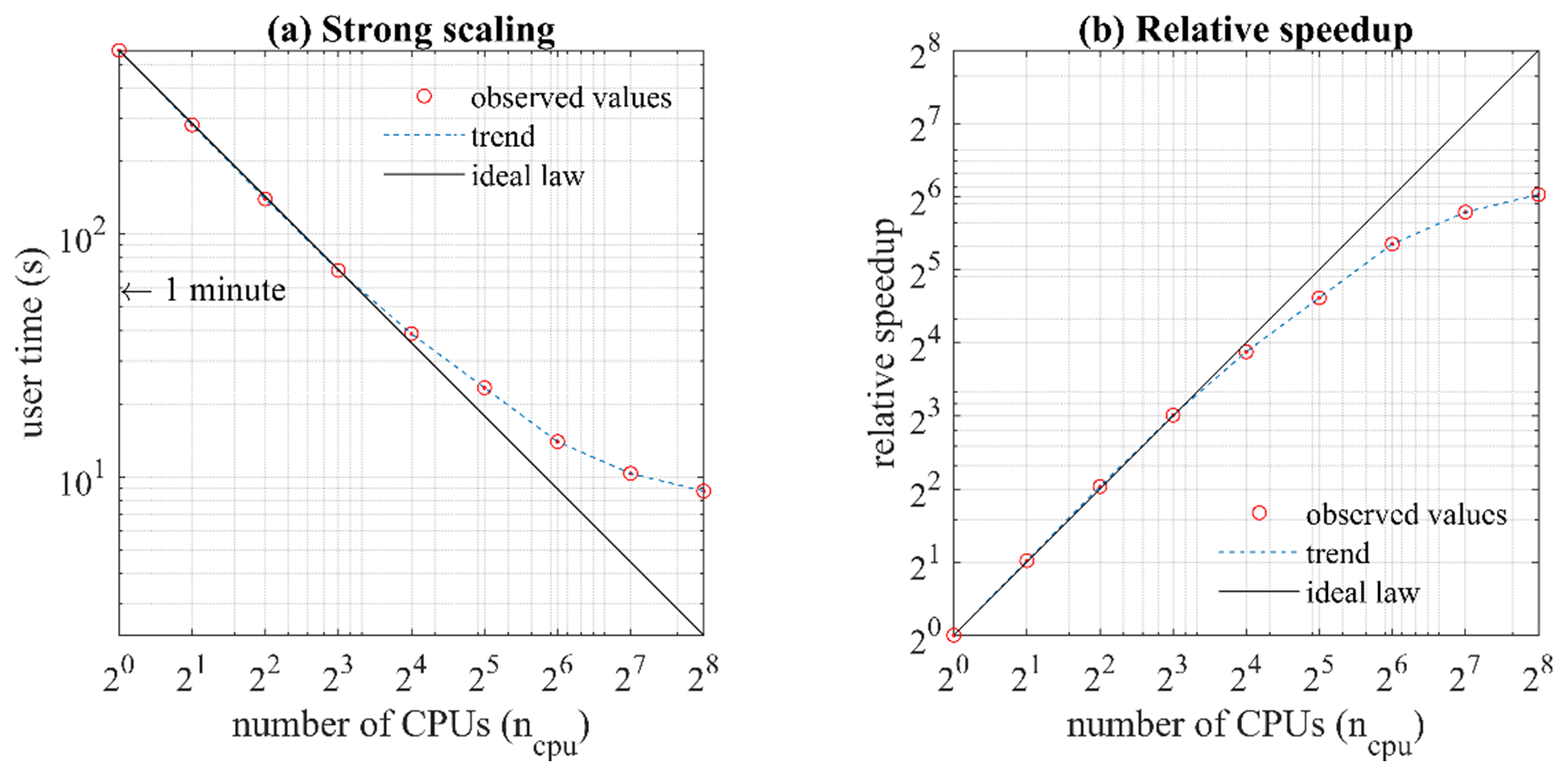
Figure D1 Strong scaling (a), relative speedup (b), and number of elements per CPU plots for a number of CPUs equal to 1, 2, 4, 8, 16, 32, 64, 128, 256, and 512. The line marked “ideal law” indicates perfect scalability for the tests that were performed.

Figure D1a shows the parallelisation efficiency. It reveals that the scaling is nearly perfect for up to 16 CPUs, that it is very good for 32 CPUs, and that it deteriorates above 64 CPUs. This corresponds to relative speedups (ratio between run time for a single CPU and a given number of CPUs) of about 14.5, 25, and 40 (Fig. D1b), respectively. For the cases using 64, 128, and 256 CPUs, speedup increases from 40 to 65, indicating that overhead inter-processor communication time for n_cpu≥64 increasingly impacts the total computation time for this (small) problem size. This is noticeable in Fig. D1a and b, as both curves seem to adopt an asymptotic behaviour for the largest numbers of CPUs. This illustrates the deterioration of performances due to inter-processor communications (Kumar et al., 1994). The deterioration of performances due to inter-processor communications is due to the number of elements (or model cells) processed by each CPU becoming smaller, while the number of elements involved in communications increases; ultimately, the time spent in pure computations in each core becomes smaller than the time spent in inter-processor communications.

The efficiency curves (e.g. Fig. D1a and b) allow us to determine the minimum number of elements per CPU that run efficiently (Hammond and Lichtner, 2010). The case of n_cpu=64 marks an inflection point in Fig. D1b, corresponding to point of diminishing return equal to a number of element per CPUs of 512. This indicates that for this particular configuration, it is preferable to run inversions with n_cpu≤64 to maximise parallel efficiency. For better understanding and interpretation of scaling and speedup, we repeat that the number of elements n_el per CPU as a function of n_cpu is as follows:

$$\begin{array}{}\text{(D1)}& n_{\text{el}}={\displaystyle \frac{N_{\mathrm{x}}{N}_y{N}_z}{n_{\text{cpu}}}}.\end{array}$$

As a general rule, we recommend respecting the condition of n_el≥512. For a smaller number of elements, the allocated resources are used in a suboptimum manner. Note that the memory requirements vary proportionally with N_xN_yN_zN_data=n_mn_d, and thus no Jacobian matrix compression is used.

Appendix E: Matrix formulation of least-squares problem and resolution of the inverse problem

This Appendix introduces the matrix formulation of Eq. (5) and its resolution.

We can write the system of equations to be solved in the least-squares sense as follows.

$$\begin{array}{}\text{(E1)}& \left[\begin{array}{c}\mathbf{S}\mathit{m}\\ {\mathit{\alpha }}_{\mathrm{m}}{\mathbf{W}}_{\mathrm{m}}\mathit{m}\\ {\mathit{\alpha }}_{\mathrm{g}}{\mathbf{W}}_{\mathrm{g}}\mathrm{\nabla }\mathit{m}\\ {\mathit{\alpha }}_{\text{pe}}{\mathbf{W}}_{\text{pe}}P\left(\mathit{m}\right)\\ {\mathit{\alpha }}_{\mathrm{x}}{\mathbf{W}}_{\mathrm{x}}(\mathrm{\nabla }{\mathit{m}}^{\left(\mathrm{1}\right)}\times \mathrm{\nabla }{\mathit{m}}^{\left(\mathrm{2}\right)})\\ {\mathit{\alpha }}_{\mathrm{a}}{\mathbf{W}}_{\mathrm{a}}\mathit{m}\end{array}\right]=\left[\begin{array}{c}\mathit{d}\\ {\mathit{\alpha }}_{\mathrm{m}}{\mathbf{W}}_{\mathrm{m}}{\mathit{m}}_{\text{pr}}\\ \mathrm{0}\\ {\mathit{\alpha }}_{\text{pe}}{\mathbf{W}}_{\text{pe}}{\mathit{P}}_{\max }\\ \mathrm{0}\\ {\mathit{\alpha }}_{\mathrm{a}}{\mathbf{W}}_{\mathrm{a}}(\mathit{z}-\mathit{u})\end{array}\right]\end{array}$$

At iteration k, the system of the equation is linearised around the current model. It is solved for the optimum update of the current model m_k model update as described below. Models ${\mathit{m}}_k^{\left(\mathrm{1}\right)}$ and ${\mathit{m}}_k^{\left(\mathrm{2}\right)}$ are set accordingly with the type of inversion considered.

In Tomofast-x, depth-weighting D is applied as a sensitivity matrix preconditioner. The resulting system is solved using the LSQR algorithm (Paige and Saunders, 1982) as follows.

$$\begin{array}{}\text{(E2)}& \begin{array}{rl}& \left[\begin{array}{c}{\mathit{D}}^{-\mathrm{1}}\mathbf{S}\\ {\mathit{\alpha }}_{\mathrm{m}}{\mathit{D}}^{-\mathrm{1}}{\mathbf{W}}_{\mathrm{m}}\\ {\mathit{\alpha }}_{\mathrm{g}}{\mathit{D}}^{-\mathrm{1}}{\mathbf{W}}_{\mathrm{g}}\frac{\partial \mathrm{\nabla }{\mathit{m}}_k}{\partial \mathit{m}}\\ {\mathit{\alpha }}_{\text{pe}}{\mathit{D}}^{-\mathrm{1}}{\mathbf{W}}_{\text{pe}}{P}^{\prime }\left({\mathit{m}}_k\right)\\ {\mathit{\alpha }}_{\mathrm{x}}{\mathit{D}}^{-\mathrm{1}}{\mathbf{W}}_{\mathrm{x}}\frac{\partial }{\partial \mathit{m}}(\mathrm{\nabla }{\mathit{m}}_k^{\left(\mathrm{1}\right)}\times \mathrm{\nabla }{\mathit{m}}_k^{\left(\mathrm{2}\right)})\\ {\mathit{\alpha }}_{\mathrm{a}}{\mathit{D}}^{-\mathrm{1}}{\mathbf{W}}_{\mathrm{a}}\end{array}\right]\mathrm{\Delta }{\stackrel{\mathrm{‾}}{\mathit{m}}}_{k+\mathrm{1}}\\ & =-\left[\begin{array}{c}g\left({\mathit{m}}_k\right)-\mathit{d}\\ {\mathit{\alpha }}_{\mathrm{m}}{\mathbf{W}}_{\mathrm{m}}({\mathit{m}}_k-{\mathit{m}}_{\mathrm{pr}})\\ {\mathit{\alpha }}_{\mathrm{g}}{\mathbf{W}}_{\mathrm{g}}\mathrm{\nabla }{\mathit{m}}_k\\ {\mathit{\alpha }}_{\text{pe}}{\mathbf{W}}_{\text{pe}}\left(P\right({\mathit{m}}_k)-{\mathit{P}}_{\text{max}})\\ {\mathit{\alpha }}_{\mathrm{x}}{\mathbf{W}}_{\mathrm{x}}(\mathrm{\nabla }{\mathit{m}}_k^{\left(\mathrm{1}\right)}\times \mathrm{\nabla }{\mathit{m}}_k^{\left(\mathrm{2}\right)})\\ {\mathit{\alpha }}_{\mathrm{a}}{\mathbf{W}}_{\mathrm{a}}({\mathit{m}}_k-{\mathit{z}}^k+{\mathit{u}}^k)\end{array}\right]\end{array}\end{array}$$

At each kth inversion cycle, we solve this system of equations and calculate the model update the model as follows:

$$\begin{array}{}\text{(E3)}& \mathrm{\Delta }{\mathit{m}}_{k+\mathrm{1}}={\mathit{D}}^{-\mathrm{1}}\mathrm{\Delta }{\stackrel{\mathrm{‾}}{\mathit{m}}}_{k+\mathrm{1}}.\end{array}$$

The model m_k can then be updated to obtain m_k+1.

$$\begin{array}{}\text{(E4)}& {\mathit{m}}_{k+\mathrm{1}}={\mathit{m}}_k+\mathrm{\Delta }{\mathit{m}}_{k+\mathrm{1}}\end{array}$$

Following Ogarko et al. (2021a), u⁰=0 and z⁰=0. The updated ADMM variables z^k+1 and u^k+1 are calculated using the ADMM algorithm introduced by Boyd (2010):

$$\begin{array}{}\text{(E5)}& {\displaystyle }{\mathit{z}}^{k+\mathrm{1}}& {\displaystyle }={\mathit{\pi }}_B({\mathit{m}}_{k+\mathrm{1}}+{\mathit{u}}^k),\text{(E6)}& {\displaystyle }{\mathit{u}}^{k+\mathrm{1}}& {\displaystyle }={\mathit{u}}^k+{\mathit{m}}_{k+\mathrm{1}}-{\mathit{z}}^{k+\mathrm{1}},\end{array}$$

where π_B is a projection onto the bounds B such that

$$\begin{array}{}\text{(E7)}& {\displaystyle }{\mathit{\pi }}_B\left(x\right)& {\displaystyle }=\left[{\mathit{\pi }}_{B_{\mathrm{1}}}\right(x_{\mathrm{1}}),{\mathit{\pi }}_{B_{\mathrm{2}}}(x_{\mathrm{2}}),\mathrm{\dots },{\mathit{\pi }}_{B_n}(x_n\left)\right]\text{, with}\text{(E8)}& {\displaystyle }{\mathit{\pi }}_{B_i}\left(x_i\right)& {\displaystyle }=\arg \underset{y\in B_i}{min}\Vert x_i-y{\Vert }_{\mathrm{2}},\end{array}$$

The value of the starting model m⁰ is provided by the user.