An overview of the Western United States Dynamically Downscaled Dataset (WUS-D3)

Predicting future climate change over a region of complex terrain, such as the western United States (US), remains challenging due to the low resolution of global climate models (GCMs). Yet the climate extremes of recent years in this region, such as floods, wildfires, and drought, are likely to intensify further as climate warms, underscoring the need for high-quality and high-resolution predictions. Here, we present an ensemble of dynamically downscaled simulations over the western US from 1980–2100 at 9 km grid spacing, driven by 16 latest-generation GCMs. This dataset is titled the Western US Dynamically Downscaled Dataset (WUS-D3).

We describe the challenges of producing WUS-D3, including GCM selection and technical issues, and we evaluate the simulations' realism by comparing historical results to temperature and precipitation observations. The future downscaled climate change signals are shaped in physically credible ways by the regional model's more realistic coastlines and topography. (1) The mean warming signals are heavily influenced by more realistic snowpack. (2) Mean precipitation changes are often consistent with wetting on the windward side of mountain complexes, as warmer, moister air masses are uplifted orographically during precipitation events. (3) There are large fractional precipitation increases on the lee side of mountain complexes, leading to potentially significant changes in water resources and ecology in these arid landscapes. (4) Increases in precipitation extremes are generally larger than in the GCMs, driven by locally intensified atmospheric updrafts tied to sharper, more realistic gradients in topography. (5) Changes in temperature extremes are different from what is expected by a shift in mean temperature and are shaped by local atmospheric dynamics and land surface feedbacks. Because of its high resolution, comprehensiveness, and representation of relevant physical processes, this dataset presents a unique opportunity to evaluate societally relevant future changes in western US climate.

1 Introduction

Predicting climate change on a regional level is critical for assessing its societal impacts, such as changes to water resources, flooding, drought, heat waves, wildfire, and windstorms. Current-generation global climate models (GCMs) are ill-equipped for this task due to their coarse grid spacing (on the order of 1° longitude and latitude). This prevents GCMs from representing complex terrain and from resolving small-scale meteorological phenomena that define the local hydroclimate. To counter this limitation, a regional climate model (RCM) may be used to dynamically downscale the GCM projections over a limited area. The resulting high-resolution output allows us to study future weather- and climate-relevant processes that may unfold across a region of complex terrain and gain physical insights into the land–atmosphere drivers of regional climate change. Moreover, the output can be used to drive land surface, hydrological, and fire models under future climate conditions.

The western United States (WUS) is a particularly complex natural laboratory for studying the heterogeneous patterns of historical climate and future climate change. It consists of major mountain ranges, deserts, shrublands, temperate forests, plains, and a complex coastline. It is affected by diverse atmospheric phenomena, such as extratropical cyclones, atmospheric rivers, persistent blocking highs, the North American Monsoon, summertime convective storms, wildfire-related downslope winds, and cooling coastal breezes. The complex interplay of these phenomena with local topography makes it impossible for GCMs to represent the diversity of microclimates within the WUS and how they may uniquely respond to larger-scale climate change. In general, GCMs project midlatitude wetting to the north of the region and subtropical drying to the south but with disagreement on where within the WUS the transition occurs (Meehl et al., 2007; Neelin et al., 2013). Moreover, intensified interannual swings between extremely wet and extremely dry years (i.e., “whiplash”) are projected in parts of the region (Swain et al., 2018; Chen et al., 2022). In recent years the WUS has experienced catastrophic weather and climate events, such as the southwestern US drought (Mankin et al., 2021; White et al., 2023), record-breaking floods in California in 2017 (White et al., 2019) and 2023, and the unprecedented 2021 heat wave in the Pacific Northwest (White et al., 2023). In a warming climate, all these extreme events are likely to be intensified. Thus, dynamical downscaling of future GCM projections over the WUS can provide a unique insight into how large-scale climate change may interact with its complex terrain and diverse meteorological phenomena.

Direct dynamical downscaling of GCMs is far less common than that driven by historical reanalyses (Liu et al., 2017, 2011; Rahimi et al., 2022; Rasmussen et al., 2011, 2014; Norris et al., 2019, and many, many others) due to the fact that historical reanalyses tend to more reliably contain the requisite data to drive RCMs (Bruyère et al., 2014; Coppola et al., 2020, 2021; Huang et al., 2020, 2021; Komurcu et al., 2018; Wang and Kotamarthi, 2015, 2013; Zobel et al., 2018, 2017; Bukovsky and Karoly, 2011; Bukovsky et al., 2021; Mearns et al., 2012; Scalzitti et al., 2016). Further, since dynamical downscaling uses the laws of physics to arrive at the high-resolution end product, it can be superior to other purely statistical-based downscaling methods. For example, dynamical downscaling does not explicitly assume stationarity (Lanzante et al., 2018) in the creation of future projections, as with other forms of downscaling (e.g., statistical); the parameterization choices within RCMs do contain empirically derived assumptions that are not completely free of time stationarity. Dynamical downscaling can however be used to tie explicitly simulated extreme weather events to the governing large-scale dynamics simulated within their driving GCMs. Additionally, RCMs can solve for the full complement of physical quantities relevant to climate that are otherwise not available in statistical downscaling, which typically focuses on a small set of variables. For example, statistically downscaled precipitation and temperature data products, even when obtained using multivariate relationships, may contain no information about water vapor content, surface pressure, cloud depth, etc. Finally, the use of physics to arrive at the downscaled result means that feedbacks between the landscape and the overlying atmosphere, as well as other land and atmosphere processes, may be effectively simulated (e.g., the snow albedo feedback).

There are three significant barriers to using RCMs to dynamically downscale GCMs: (1) RCMs require sub-daily 3-D variables as initial and boundary conditions, which are not typically sufficiently archived in GCM databases; (2) RCM configurations may not be designed to ingest GCM data as boundary conditions; and (3) it is extremely computationally expensive. Because of these barriers, dynamical downscaling of full GCM ensembles (e.g., the Coupled Model Intercomparison Project Phase 6; CMIP6) at landscape-resolving (∼ 10 km) grid spacings generally remains out of reach.

Despite these barriers, we present results from 16 new dynamically downscaled CMIP6 simulations over 11 WUS states, including the whole of the Western Electricity Coordinating Council (WECC) region, comprising the Western US Dynamically Downscaled Dataset (WUS-D3). These simulations span 1980–2100, combining the historical and Shared Socioeconomic Pathway (SSP) output for each GCM. Downscaling a wide variety of CMIP6 models yields a diverse suite of possible future climates over the WUS at a landscape-resolving scale (9 km grid spacing). In the following sections, we present our methodology and technical challenges encountered, as well as a characterization of the historical performance and future change signals from our dataset.

2 Methodology

2.1 WRF setup

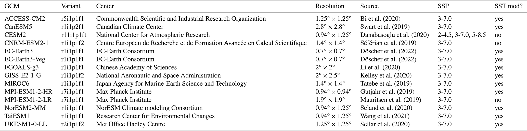
We use the Weather Research and Forecasting (WRF) model version 4.1.3 (Skamarock et al., 2019) to dynamically downscale the simulations of 14 CMIP6 GCMs (Table 1) from 1980–2100. In each simulation, historical forcings were applied up to 2014 and then the forcings associated with the SSP3-7.0 scenario thereafter. SSP3-7.0 is a high-emissions scenario in which greenhouse gas emissions double by end of century (O'Neill et al., 2016). We also downscale one GCM's (CESM2) SSP2-4.5 and SSP5-8.5 projections. In these scenarios, emissions remain roughly constant until 2050 before falling thereafter and triple by end of century, respectively.

Table 1 List of GCMs dynamically downscaled in this study. Approximate near-equatorial latitude–longitude resolutions are given. The rightmost column titled “SST mod” indicates whether or not our GoC entrance-region-based SST extrapolation is utilized.

WRF is configured as was documented for a related downscaling of the ECMWF Fifth Generation Reanalysis (ERA5; Hersbach et al., 2020) in Rahimi et al. (2022; WRF-ERA5). We downscale each GCM year separately and in parallel; at the beginning of each downscaling period (on 1 August ), the RCM is initialized to the driving GCM state. In this way, an N-year simulation can be completed in the same wall clock time as a 1-year experiment. For each year of integration, we choose the beginning of the retained WRF output for analysis to coincide with minimum snowpack across the WUS (1 September). This approach produces 1 month of spin-up for the land surface. Thus, WRF is initialized on 1 August to surface and 3-D data from each GCM and integrated through 1 September of the following year (13 months, including the spin-up month) on 39 atmospheric levels. This approach is similar to that of Zobel et al. (2018, 2017), who also initialized WRF experiments at yearly intervals but only included 1 d of model spin-up. Despite our 1-month spin-up, soil moisture, land surface fluxes, and streamflow may still suffer from biases due to imperfect soil texture categories and their associated hydrophysical properties (Dennis and Berbery, 2021). However, because soil texture is a necessary component of the land surface model and these underlying datasets are imperfect, these effects are somewhat unavoidable without massive regional calibration. WRF's parallelization procedure, which is advantageous for executing simulations in weeks instead of years, is performed to the detriment of time continuity in simulating the surface and subsurface runoff, as well as energy fluxes, with high precision. The consequences of this choice will be expanded upon in Sect. 2.6.

Atmospheric carbon dioxide and methane concentrations vary yearly in our simulations based on northern hemispheric mean values from input4MIPs (Durack et al., 2017). Prior to 2015, CMIP6 historical values are prescribed. From 2015 onward, these values are taken from the SSP3-7.0 scenario, except for the alternate SSP CESM2 experiments. WRF's radiative code is modified to enable concentrations to be manually inputted; this modification is no longer needed as of WRF version 4.4.2. Because coupling WRF to an atmospheric chemistry model is 6–20 times more computationally expensive, interactive aerosol forcings were not explicitly considered in our study. Further, historical-era 21-category land-use and land-coverage (LULC) information from the Moderate Resolution Imaging Spectroradiometer is used in all experiments. Since CMIP-projected LULC changes were not implemented in WUS-D3, the anthropogenic forcings considered in this study stem directly from carbon dioxide and methane concentrations and indirectly from all greenhouse gas, aerosol, and LULC forcings in the forcing GCMs at the lateral boundaries.

We dynamically downscale all GCMs to two grids of 45 and 9 km grid spacing (Fig. 1). On the parent 45 km grid, the horizontal winds, temperature, and geopotential height are relaxed (relaxation coefficient of 0.0003 s⁻¹) to their respective GCM-simulated fields above the planetary boundary layer via spectral nudging for wavelengths greater than 1500 km. Smaller waveforms are allowed to evolve freely on the WRF grid (Spero et al., 2014). This approach is designed to reduce internal model drift away from the GCM state. One-way nesting is then used to dynamically downscale the 45 km result to the 9 km grid, on which spectral nudging is not implemented. The 9 km grid encompasses the entirety of the WECC's US coverage area. For all nests, a sponge layer of five grid points is used.

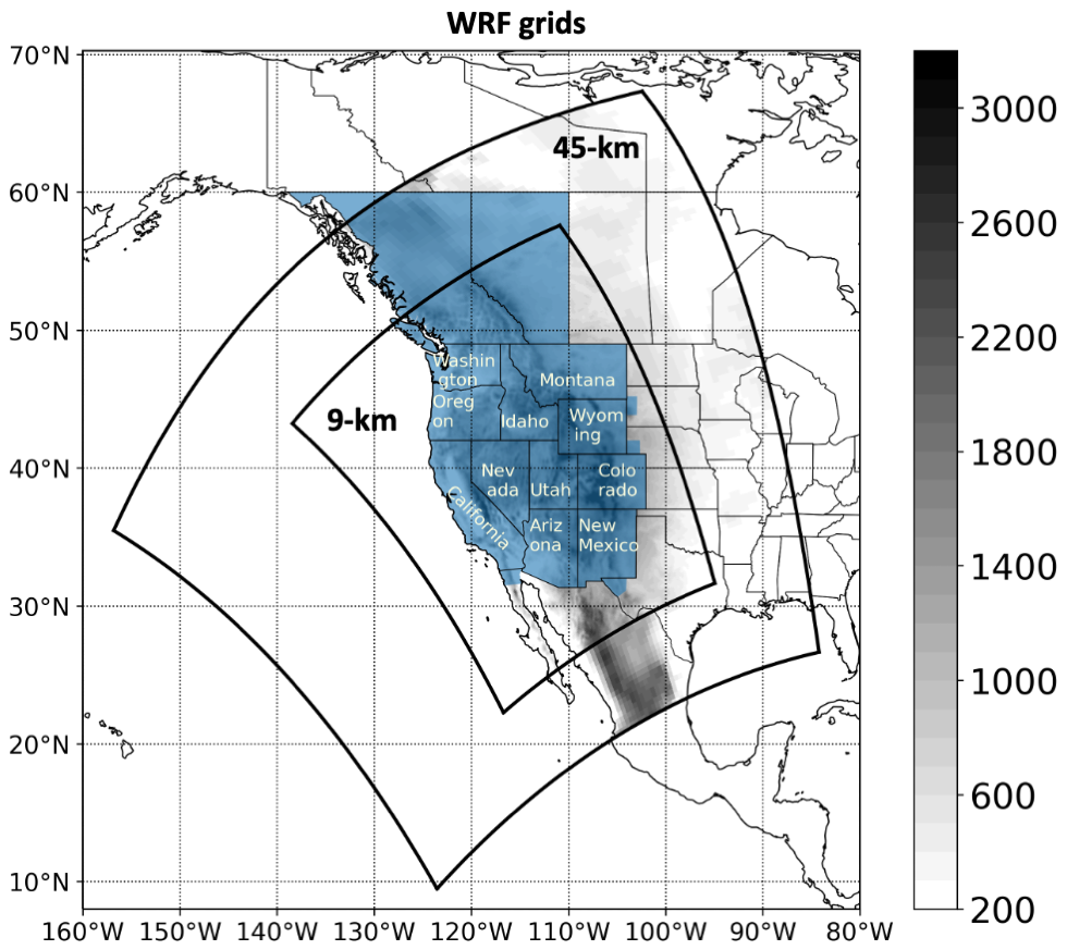
Figure 1 WRF grids used in this study. Topography [m] is shaded to its highest resolution, and the blue shading indicates the Western Electricity Coordinating Council (WECC) coverage area.

The lateral boundary conditions are updated at 6-hourly intervals, and adaptive time stepping is used. Convective precipitation is parameterized following Tiedtke (1989) and Zhang et al. (2011). P3 microphysics is used (Morrison and Milbrandt, 2015), shortwave and longwave radiation schemes of Iacono et al. (2008) are implemented, and the Noah land surface model with multi-parameterizations (Noah-MP) is used (Niu et al., 2011).

2.2 GCM selection

Prioritizing SSP3-7.0 with an end-of-century radiative forcing of 7 W m⁻², we selected 14 GCMs (Table 1) based on three criteria: (i) their skill in simulating important processes that govern western North American climate over the historical (1980–2010) period, (ii) their collective representativeness of the broader CMIP6 ensemble spread in future temperature and precipitation responses, and (iii) data availability. Aspects considered in the GCM evaluation included the following.

1. Large-scale meteorology associated with Santa Ana and Diablo winds. This is important for extreme wind and fire risk across the southwestern US. We use this metric to minimize the usage of GCMs which simulate a distorted portrayal of the Pacific High.

2. The El Niño–Southern Oscillation (ENSO). ENSO is well-known to modulate the interannual variability in precipitation and temperature across the western US. We use this metric to prioritize GCMs which adequately capture the ENSO–western US teleconnection.

3. Northern Hemisphere blocking and circulation (Simpson et al., 2020). Wave characteristics, both over climate and synoptic timescales, are directly related to the variability in precipitation across the WUS. We use this metric, for instance, to ensure that GCMs are not down-selected if they are too progressive in their simulation of midlatitude waves.

4. Landfalling jet characteristics. Atmospheric rivers are responsible for most of the west-coast precipitation. As such, we only select GCMs that demonstrate superior performance in their landfalling position and tilt.

5. GCM-simulated surface air temperature and precipitation. While these variables can be incorrectly simulated in GCMs despite the more-or-less correct treatment of their local driving processes, which may be more important for driving a regional climate model, we include these variables to account for the relationships between the GCM-simulated processes and GCM-simulated surface temperature and precipitation profiles.

6. Extreme precipitation across California. Generally, extreme precipitation events in California are driven by large-scale synoptic events (described by column water vapor, 500 hPa geopotential, and upper-tropospheric wind speeds). These large-scale patterns can have ramifications for weather and climate as they propagate downstream; hence we include an evaluation of bias in these fields for our GCM selection.

7. Regional wind shear. Wind shear helps to modulate the lifetime of precipitation systems through storm-scale organization and is a measure for the larger-scale background baroclinicity, which is important for storm tracks. We thus evaluate its bias.

The ranking system is described in Krantz et al. (2021), and the process of choosing GCMs to downscale based on climate-data-user needs and locally relevant atmospheric processes is described in Goldenson et al. (2023). To emphasize, being subject to these selection processes, the GCMs downscaled in this study span the range of future changes in temperature and precipitation from CMIP6 across the WUS.

For more details on the GCM selection process, we refer readers to Krantz et al. (2021). However, we highlight that temporal and spatial variability was considered in ranking a preferred set of GCMs to downscale. Specifically, the time variability of ENSO and high-frequency synoptic variability of landfalling waves are considered, while the spatial variability of the California precipitation mode (Chen et al, 2021) was factored into our analyses via the identification of where the geopotential anomalies exist upstream of the WUS on extreme precipitation days. Additionally, our metrics per Simpson et al. (2020) consider jet stream landfall position bias. Finally, Krantz et al. (2021) performed a variance decomposition using empirical orthogonal functions to reduce the effects of metric redundancy, weighting them accordingly in the final rankings of GCMs.

We only dynamically downscale GCMs with the following outputs archived on the Earth System Grid Federation system: 3-D atmospheric temperature (ta), horizontal winds (ua and va), specific humidity (hus), surface pressure (ps), soil layer specific temperature and water content (tsl and mrsol, respectively), and sea surface temperature (SST; tos). Furthermore, we only dynamically downscale GCMs with 6-hourly instantaneous atmospheric outputs defined on native model levels (“6hrLev”) rather than on isobaric surfaces (“6hrPlevPt”). Generally, 6hrPlevPt GCM outputs are only defined on 3–10 pressure surfaces, which may be problematic for atmospheric phenomena characterized by more granular vertical structures. In testing, we found that this vertical resolution can have a large impact on the downscaled solution in cases where 6 versus 23 isobaric levels were used.

Additionally, we require that the full time series of SSTs be available in GCM outputs. These SSTs are then prescribed in WRF to update daily, which may be problematic for atmospheric processes subject to a strong atmospheric–ocean coupling evolving on sub-daily timescales. To bypass this issue, we tested using a slab ocean model in WRF. With time, strange artifacts in the SST and outgoing longwave radiation fields gradually developed, so slab ocean physics were not enabled, and its use is discouraged for simulations on regional climate timescales (Ming Chen, personal communication, https://forum.mmm.ucar.edu/threads/weird-pixilated-skin-temperatures-when-using-sf_ocean_physics-1.12693 (last access: April 2023), 2023). Daily SSTs are available for most GCMs, except for FGOALS-g3 and GISS-E2-1-G, which only made monthly SST outputs available. Thus, in the cases of FGOALS-g3 and GISS-E2-1-G, linear interpolation is used to upsample monthly mean SSTs (assumed to be valid at the midpoint of each month) to daily values.

2.3 Sea surface temperatures in the Gulf of California

SSTs in the Gulf of California (GoC) are known to modulate the North American Monsoon, which provides roughly a third of Arizona and New Mexico's annual precipitation (Mitchell et al., 2002). However, the GoC is poorly resolved in CMIP6 GCMs; in the best case, the GoC is expressed as a subtle bay that barely intrudes into the North American continent. As a result, there is generally no SST information from GCMs across the GoC that can be used to directly prescribe SSTs in the WRF-resolved GoC. An additional problem is that the adjacent open Pacific SSTs are on average about 10 K lower and undergo less seasonal variability than in the GoC (Fig. 2). Hence, linearly extrapolating from the adjacent open Pacific to the GoC would produce a representation of GoC SSTs that is clearly unphysical. Fortunately, there are predictable relationships in ERA5 between the climatological GoC entrance region temperature (Fig. 2c), which can be taken directly from GCMs, and the along-axis GoC SST gradient (Fig. 2d), which can be used to produce reasonable SSTs within the GoC. Thus, in most GCMs, we apply the following linear extrapolation to estimate GoC SSTs based on the entrance region SSTs:

$$\begin{array}{}\text{(1)}& T_{\mathrm{GoC}}=-{\left.{\displaystyle \frac{\partial T}{\partial n}}\right]}_{\mathrm{ERA}\mathrm{5}}\left(n\right)+T_{\mathrm{entry},\mathrm{GCM}},\end{array}$$

where ${\left.\frac{\partial T}{\partial n}\right]}_{\mathrm{ERA}\mathrm{5}}$ is the monthly varying climatological GoC temperature gradient from ERA5 and is always positive, n is the along-axis GoC coordinate (pointing towards the northwest), and T_entry,GCM is the GoC entrance temperature which is resolved in GCMs. The relevant regions are outlined in Fig. 2a. To our knowledge, the difficulty in dealing with SSTs in coastal estuaries and gulfs has not been generally addressed in regional climate modeling efforts, and this is the first time that a physically based mathematical relationship has been used to address this issue across this region.

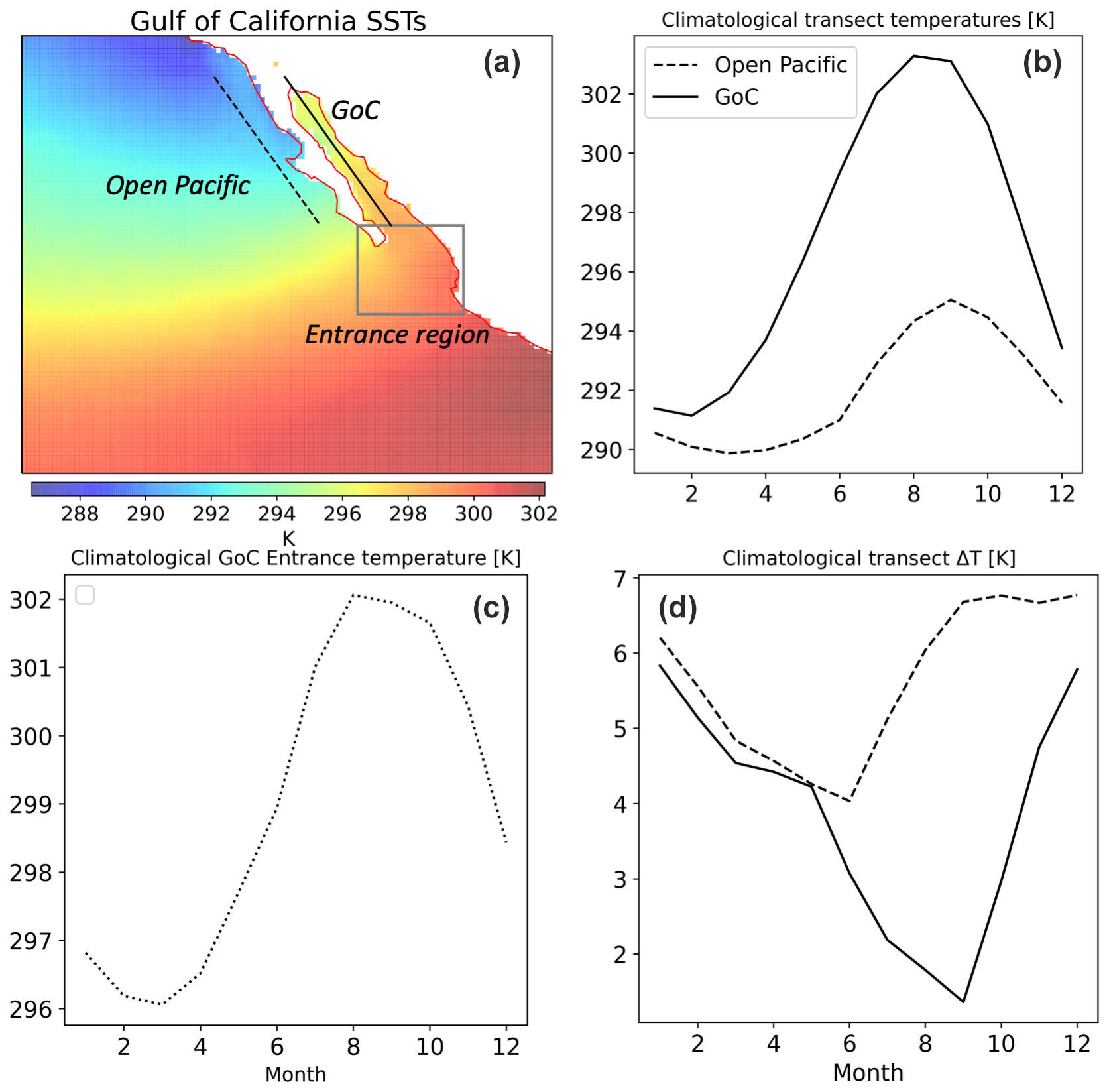
Figure 2 (a) Climatological (1980–2014) mean SSTs from ERA5 along with transects across the Gulf of California (GoC; solid black curve) and open Pacific (dashed black curve). The gray bounded zone is our GoC entrance region. Panel (b) shows the latitudinally weighted transect mean temperatures from the open Pacific and GoC. Panel (c) shows the area-weighted GoC entrance region temperature, while panel (d) depicts the temperature gradient along the open Pacific and GoC transects from northwest to southeast.

We apply the above linear extrapolation to all GCMs, except CESM2, CNRM-ESM2-1, and MPI-ESM1-2-LR, which were all downscaled prior to the implementation of this improvement. Consequently, for CESM2 and MPI-ESM1-2-LR, there is a spurious SST discontinuity (Fig. S1 in the Supplement). This is due to the default extrapolation routine used in WRF, which uses a nearest weighted grid point averaging approach to prescribe GoC SSTs. Thus, in the southern GoC, the default extrapolation uses the nearest GCM grid points from the warm GoC entrance region, whereas further north the closest GCM ocean grid cells are (inappropriately) taken from the open Pacific. We list the GCMs with the SST modification in the rightmost column of Table 1. The discontinuity and unrealistically low SSTs in the northern GoC in these simulations may affect the simulation of the North American Monsoon but are unlikely to affect other WUS phenomena documented in this paper. For CNRM-ESM2-1, we masked out the southern GoC to remove this discontinuity in extrapolation, leading to its SSTs being homogeneously populated by open Pacific SSTs. Despite the absence of a SST discontinuity (Fig. S1), this approximation is less physical than the improvement described above (Fig. 2).

2.4 Interpolation strategy

WRF requires all atmospheric, land, and ocean GCM inputs to be defined on a single rectilinear grid with atmospheric variables defined on isobaric surfaces. However, some GCMs' outputs are given on irregular atmospheric grids, whose latitude coordinates are not equally spaced from pole to pole. FGOALS-g3 for instance is characterized by ∼ 5° latitudinal grid spacing near the poles and ∼ 2° grid spacing near the Equator. Thus, for the GCMs without a native rectilinear grid, we bilinearly interpolate the output to rectilinear grids with grid lengths defined by their respective absolute minimum latitude or longitude grid spacing. This technique preserves the smallest-scale features resolved on the native GCM grid.

Since GCMs use different land surface models (LSMs) containing differently defined vertical coordinates, we generally interpolate volumetric soil moisture and soil temperature from the native LSM levels to 3.5, 14, 64, and 195 cm. In instances where vertical interpolation was not used, we used the GCM's native grid soil information. We computed volumetric soil moisture by dividing layer total water content (CMIP6 variable mrsol) by the layer thickness and the density of liquid water. GCM soil fields were generally available daily.

2.5 Other technical challenges

In this section, we present additional technical challenges and known issues in the downscaled data. First, WRF is not designed to ingest GCM inputs that are, depending on the modeling center, defined on different vertical coordinates. For instance, CESM2 uses a hybrid-pressure, FGOALS-g3 a sigma, and UKESM1-0-LL a hybrid-height vertical coordinate system. As a result, unique routines had to be developed for each GCM to convert their model level output to WRF-usable inputs on isobaric pressure surfaces. Further, MPI-ESM1-2 simulations had to be converted from NetCDF-4 to NetCDF-4 Classic in order for input-output processing times to be tractable in binary processing. These issues alone prevented the development of a one-size-fits all routine to preprocess GCM outputs for ingestion by WRF. These issues were compounded by the fact that some GCMs, such as UKESM1-0-LL and ACCESS-CM2, contain staggered outputs on their native Arakawa C-grids.

Second, 6hrLev GCM atmospheric fields are generally provided at 00:00, 06:00, 12:00, and 18:00 UTC. However, for the entire FGOALS-g3 and historical (1980–2014) component of the NorESM2-MM experiments, data were provided at 03:00, 09:00, 15:00, and 21:00 UTC. For FGOALS-g3, we simply integrated all experiments from 1 August 1980 at 03:00 UTC through 1 September 2100 at 03:00 UTC. For NorESM2-MM, however, we linearly interpolated the historical GCM data to 00:00, 06:00, 12:00, and 18:00 UTC before downscaling. As a further aside, since UKESM1-0-LL uses a 360 d calendar, we had to modify WRF's source code accordingly. WRF is designed by default to function with proleptic Gregorian calendars (e.g., ERA5, MPI-ESM1-2-LR, EC-Earth3-Veg), but we compiled the model with no-leap calendars for other GCM experiments (e.g., CESM2, GISS-E2-1-G, TaiESM1).

2.6 Spin-up strategy consequences

Despite 1 month of spin-up in parallelized yearly WRF experiments, our adopted spin-up strategy neglects high-resolution soil memory on timescales greater than 1 month. This assumption may be particularly problematic across regions where a transient simulation is necessary to equilibrate the soil conditions to a state which properly resolves the local-scale land–atmosphere coupling. For instance, some grid points do not see complete meltout of snow by 31 August 1993, but since data are retained from 1 September 1993 onwards, there are instances where discontinuities in surface snow coverage exist. This leads to discontinuities in surface energy variables (e.g., sensible heating; not shown). We encourage users of WUS-D3 to be wary of this pitfall. To alleviate this discontinuity, we propose that the atmospheric temperature, precipitation, surface radiative fluxes, winds, and specific humidity from WRF be used to drive offline calibrated hydrology models that are time continuous and can be integrated much more rapidly (e.g., Bass et al., 2023). We acknowledge that this approach is inadequate across regions with a strong land–atmosphere coupling.

3 Simulation of the historical climate

Next, we present a review of simulated historical (1981–2010) precipitation and surface air temperature across the WUS. Figure 3 shows the added value introduced by dynamical downscaling in simulating these patterns, as well as the relative fidelity of the GCMs when downscaled with WRF. We compare the downscaled ensemble mean against the native-resolution GCM ensemble mean, in addition to 9 km WRF-ERA5 and observational estimates from the 4 km Parameter-elevation Regressions on Independent Slopes Model (PRISM; Daly et al., 1994). The inability of the raw GCMs to capture the complex terrain of the WUS is illustrated by major warm and cold biases over mountains and valleys, respectively. In particular, California's Central Valley is 5–7 K too cool, while the Sierra Nevada is warm biased by the same magnitude. By contrast, the dynamically downscaled simulations, whether GCM- or ERA5-driven, better resemble the regional temperature and precipitation patterns shown by PRISM. Despite this improvement, the downscaled GCM experiments are generally colder than PRISM, by as much as 5 K during part of the year in some states (Fig. 4). The annual mean spatial patterns in Fig. 3 reveal the cold biases to be predominantly over mountains. The cold bias is generally most prominent in the winter months (shown by spatial patterns in Fig. S2) but persists year-round. Additionally, dynamical downscaling generally reduces the simulated temperature spread from that of the parent GCMs, as indicated by the red circles (Fig. 4). Exceptions are noted across western states, especially in winter; we speculate that dynamical downscaling is increasing the spread proportional to the magnitude of GCM biases in temperature, winds, and SSTs, leading, when inherited by WRF, to varying magnitudes of downscaled precipitation and temperature bias. GCM bias impacts on the dynamically downscaled solution are a current core focus by our research team.

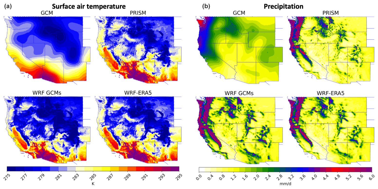
Figure 3 The 1981–2010 annual mean (a) surface air temperature [K] and (b) precipitation rate [mm d⁻¹] from the native GCMs (GCM; 14-GCM ensemble mean), dynamically downscaled ERA5 (WRF-ERA5), dynamically downscaled GCMs (WRF GCMs; 14-member ensemble mean), and PRISM. All GCM and PRISM data are interpolated from their native grids to the 9 km WRF grid.

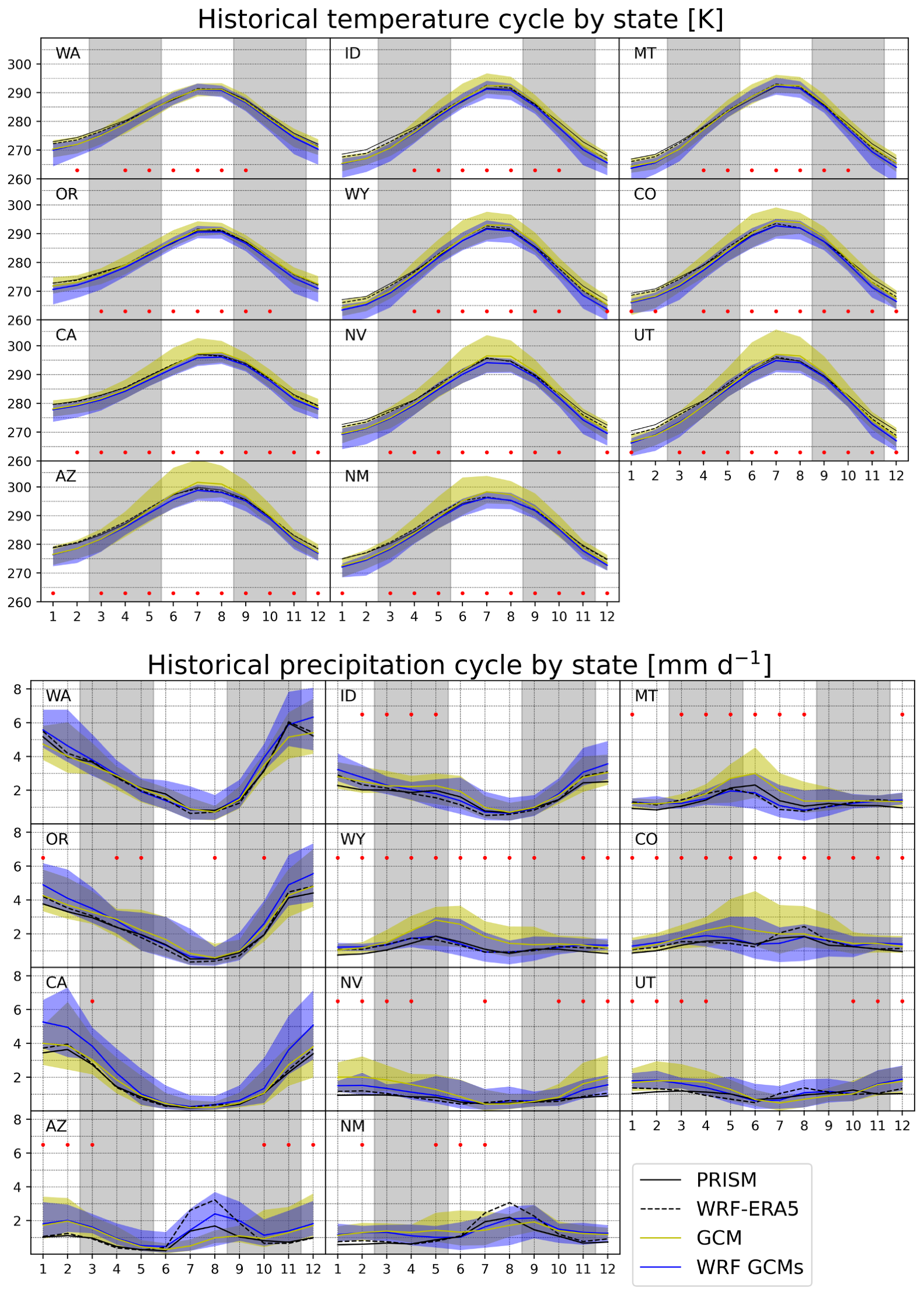
Figure 4 The 1981–2010 seasonal cycles of state mean surface air temperature [K] and precipitation [mm d⁻¹] from native GCMs (GCM), dynamically downscaled ERA5 (WRF-ERA5), dynamically downscaled GCMs (WRF GCMs; 14-member ensemble mean), and PRISM. The parent and downscaled GCM ensemble spreads are presented in yellow and blue shading, respectively. Red circles indicate months where the dynamically downscaled spread is smaller than the parental GCM spread.

The dynamically downscaled ensemble mean is generally too wet across the states of Washington, Oregon, and California (Figs. 3, 4). A preexisting wet bias in the parent GCMs is increased by downscaling, an impact seen primarily over mountains during winter (Fig. S3). These biases vary substantially within the ensemble, with individual downscaled GCMs exhibiting meaningful state-wide biases of hundreds of percent (e.g., California in May for CNRM-ESM2-1; not shown). However, the downscaled results greatly improve on large wet biases across Nevada, Colorado, Wyoming, and Montana in the parent GCMs, which are as much as 50 % in the ensemble mean across Wyoming and hundreds of percent in some GCMs. Also, across Arizona, the summertime monsoonal precipitation maximum is completely missed in all GCMs. Meanwhile, the downscaled results capture it well, albeit with some simulations that are far too wet (∼ 100 % bias) compared to PRISM. Difficulties in simulating summertime precipitation across the southwestern US have been noted in previous studies (Liu et al., 2017; Rahimi et al., 2022). To summarize, dynamical downscaling generally increases the simulated precipitation spread across Arizona, California, Oregon, and Washington whilst decreasing the spread across interior states.

In general, overly wet and cold dynamically downscaled GCMs have previously been noted across the region with a different RCM (Rastogi et al., 2022), indicating that biases in the GCM forcing data may be to blame. The effects of GCM bias propagation are being explored in Rahimi et al. (2024) and Risser et al. (2024). The absence of such large biases in WRF-ERA5 (Figs. 3, 4, and 5), which is equivalent to the downscaled GCMs except driven by ERA5, lends further evidence in support of this hypothesis.

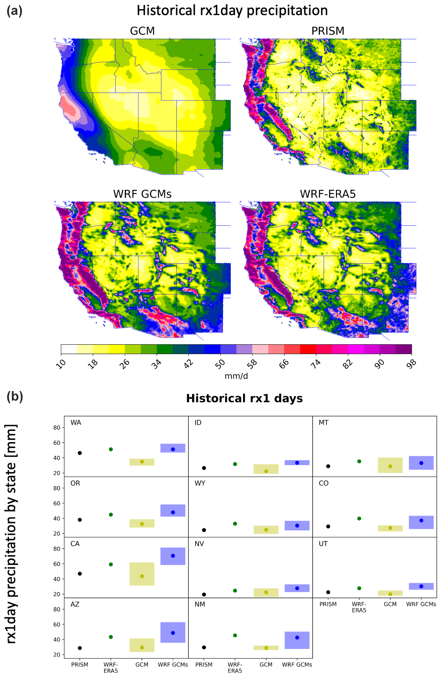
Figure 5 Historical (1981–2010) mean rx1day (annual maximum daily precipitation) precipitation amounts [mm] from native GCMs (14-GCM ensemble mean), dynamically downscaled ERA5 (WRF-ERA5), dynamically downscaled GCMs (WRF GCMs; 14-member ensemble mean), and PRISM. Panel (a) presents the spatial distribution of rx1day precipitation, while (b) presents rx1day precipitation amounts averaged across each western US state. Ensemble mean values are presented as colored circles, while the GCM spread in rx1day values is shaded. GCM data were interpolated to a 1° rectilinear grid before computations.

Finally, we evaluate historical extreme precipitation (rx1day) in WUS-D3. Dynamical downscaling markedly improves the spatial distribution of rx1day across the region compared to the parent GCMs (Fig. 5, top), as with mean precipitation (Fig. 3). Across individual states, dynamical downscaling produces rx1day magnitudes that are in many cases about double their parent GCM values, particularly across Arizona, California, Oregon, and Washington. While generally too wet compared to PRISM, downscaled simulations are much closer to the downscaled reanalysis (WRF-ERA5). We attribute the greater rx1day values in the downscaled simulations to the much better representation of topography and orographic precipitation in WRF compared to the parent GCMs. As such, the wetter behavior of WRF solutions is generally localized to the highest elevations across each state. These locations are precisely where observational uncertainties are also maximized (Lundquist et al., 2019). Thus, we characterize downscaled rx1day simulations as being wetter than PRISM rather than clearly being wet biased. Because of the rareness of rx1day events, the computation of rx1day is also sensitive to the phasing of internal climate variability, which is different in GCMs relative to PRISM and WRF-ERA5. Hence, differences between downscaled GCMs and PRISM rx1day precipitation may be partially explainable by these phasing differences.

As indicated by the shaded bars in Fig. 5, downscaling may alter the original GCM spread in simulated rx1day magnitudes. Specifically, WRF significantly increases the GCM spread in Oregon, Arizona, New Mexico, and Colorado but significantly decreases the spread in California, Nevada, Idaho, and Montana. The states with large increases in spread are generally where rx1day is more likely to occur during summer, indicating disagreements in monsoon-related extreme precipitation across downscaled results. The amplification of model uncertainty in precipitation extremes by dynamical downscaling is yet to be addressed by the regional modeling community and is a current focus of our research efforts.

4 Climate response across the western US

Next, we provide an overview of the WUS-D3's climate response to anthropogenic forcing (following SSP3-7.0). Figure 6 shows the mid-century (2030–2060; MC) and end-century (2070–2100; EC) projected changes in annual mean precipitation scattered against warming, averaged across 11 WUS states in each GCM. The native GCM projections (indicated by letters) are connected to their downscaled counterparts (indicated by circles) by thick arrows. The purpose of Fig. 6 is to illustrate the degree to which downscaling can modify the original GCM projections on regional scales.

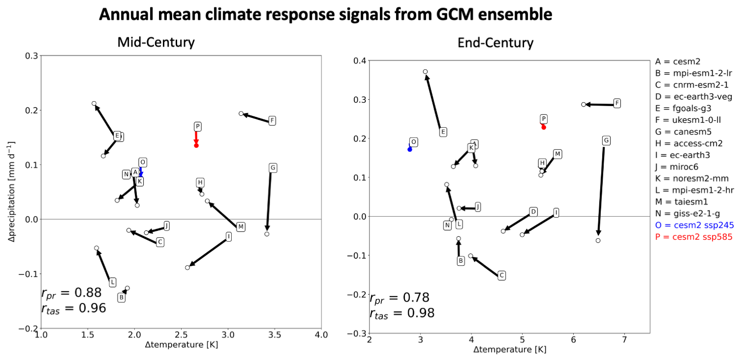
Figure 6 Future climate response for parent GCMs (indicated by lettering) and their downscaled counterparts (indicated by open circles) on the 9 km WRF grid averaged across 11 western US states. Non-colored circles are for SSP3-7.0 projections only, while blue (red) circles represent the SSP2-4.5 (SSP5-8.5) projections. Arrows point away from parent GCMs towards downscaled counterparts.

According to the downscaled ensemble, the WUS will experience 2.25 ± 0.58 K of warming by MC and 4.65 ± 14 K by EC (relative to 1980–2010). A considerably more uncertain but generally wetter future is also predicted, with an ensemble mean precipitation change of 0.039 ± 0.93 mm d⁻¹ by MC and 0.083 ± 0.13 mm d⁻¹ by EC. Despite a positive mean change, a handful of simulations suggest drying across the region (Fig. 6, right). Downscaling generally preserves the intermodel variation among the parent GCMs in the 11-state mean. For temperature change, there are correlation coefficients of 0.96 and 0.98 for MC and EC, respectively, between the raw GCM and downscaled ensembles. Correlation coefficients are lower for precipitation change but remain high: 0.88 and 0.78 for MC and EC, respectively. Regional mean GCM warming is typically modified by no more than 0.5 K. Interestingly, downscaling generally reduces warming (leftward pointing arrows). This effect is most prominent during winter and spring (Fig. S4), indicating that the much better resolution of topography and hence climatological snowpack improvements (e.g., Walton et al., 2017) in the downscaling may be reducing the overall snow albedo feedback intensity and hence the surface's temperature sensitivity to anthropogenic forcing. Summer will see the largest mean temperature increases across the WUS by EC: 5.2 ± 1.2 K in the WRF simulations compared to 5.3 ± 1.2 K in the GCMs. In contrast to temperature, downscaling does alter the regional precipitation signals significantly but not in any systematic or obviously predictable way; downscaling can either wet or dry the GCM precipitation projection. These modifications are generally no more than 0.05 mm d⁻¹, but notably CanESM5 and FGOALS-g3's projections are altered by −0.2 and +0.15 mm d⁻¹, respectively, by EC. In the case of CanESM5, this transforms strong wetting to weak drying.

4.1 Spatial patterns of temperature and precipitation change in WRF versus GCMs

Although domain mean changes are minimally unaffected by downscaling, the spatial patterns of temperature and precipitation change in the downscaled solutions are significantly different from those of the raw GCM projections (Fig. 7; individual downscaled GCM annual changes are shown in Figs. S5, S6). To account for large intermodel spread in climate sensitivity, the local warming is normalized by EC changes in global warming. A value of 2 K K⁻¹ indicates that a grid cell warms at twice the rate of the global average. Examining the upper panels of Fig. 7, large-scale spatial patterns of warming are preserved in the downscaling, but there are seasonal and local differences. Notably, we see enhanced (and likely more realistic) warming adjacent to mountainous areas of the Rockies during winter and spring and at the highest elevations of the Sierra Nevada during summer. This is primarily tied to the improved representation of topography and thus more expansive historical snow cover. We expect simulations with greater snow cover to exhibit more warming across these areas because they would be able to lose more snow under warming (Fig. S7) and therefore have a stronger snow albedo feedback (SAF; Hall, 2004; Qu and Hall, 2006; Thackeray and Fletcher, 2016). The addition of value is clear in terms of the granularity of future snow loss and subsequent impact on warming in winter and spring and is comparable to previous studies (e.g., Walton et al., 2017). However, enhanced summertime high-elevation warming may be somewhat overestimated due to large cold-season wet biases (Figs. 4, S3); excessive snow survives into the warm season and creates an unrealistically large snow albedo feedback effect under climate change. We also hypothesize that the lapse rate feedback (Hansen et al., 1984; Colman and Soden, 2021) may be contributing to the enhanced warming at high elevations during summertime. For example, in the GCMs, 850 hPa temperatures warm by 3.75 K across the WUS, while 300 hPa temperatures warm by 4.75 K (not shown). This enhanced warming at high altitudes likely contributes to enhanced surface warming at high elevations as well. Lastly, the downscaled ensemble exhibits enhanced warming across the interior during fall, perhaps associated with drying and a reduction in evaporative damping of surface temperature (Zhou et al., 2019).

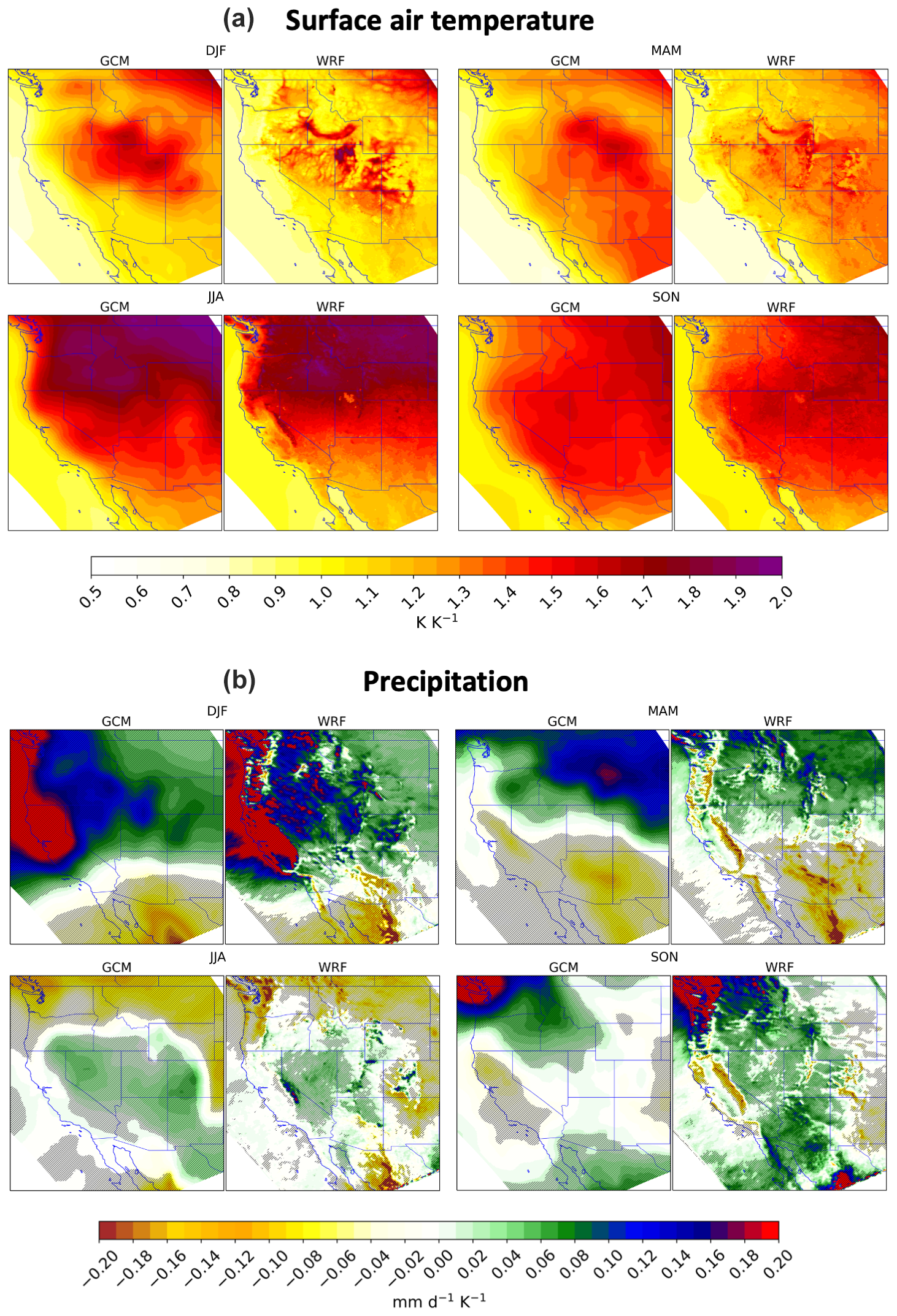
Figure 7 Ensemble mean future changes in (a) seasonal surface air temperature [K K⁻¹] and (b) precipitation per degree of global warming [mm d⁻¹ K⁻¹] from 16 downscaled GCMs. Hatching indicates statistical significance to the 95 % confidence interval when grid point distributions are subjected to a two-sided Student's t test. Stippling is not included for temperature because every grid point returns a p value smaller than 0.05.

Spatial patterns of precipitation change illustrate greater contrasts between the downscaling and GCMs across seasons (Fig. 7, lower panels). EC changes are normalized by global mean warming here to take into account the large spread in climate sensitivity among CMIP6 models and to focus attention on the components of the hydrologic response that do not simply scale with temperature. The large-scale precipitation response is generally preserved in downscaling, with statistically significant wetting (drying) in the northwestern (southwestern) US during winter and spring. The lack of statistical significance along a transition region, extending from southern California through northern Arizona and New Mexico, is symptomatic of GCM disagreement on the location of the transition of subtropical drying to midlatitude wetting (Meehl et al., 2007; Neelin et al., 2013). Consistent with other studies (e.g., Mahoney et al., 2021; Rupp et al., 2022), the downscaled ensemble appears to produce greater wetting across major WUS mountain ranges during spring and winter. The locally more intense change signal is tied to increased water vapor within atmospheric rivers and other synoptic disturbances, which interacts with WRF's more realistically simulated terrain to produce more realistic orographic uplift relative to native-resolution GCMs (Huang et al., 2020; see mean changes in vertical velocities in Fig. S8). There are also instances where WRF simulates a locally more intense drying signal compared to the native GCMs, which is also clearly linked to topography, e.g., the Sierra Nevada in autumn and spring, the upslope of the Cascades in summer, and northwestern Mexico in winter and summer.

We also examine ensemble mean fractional precipitation changes (again normalized by warming) to focus attention on where the largest changes are relative to the climatology (Fig. 8). Here, a value of −20 % K⁻¹ indicates that EC-era precipitation has decreased by 20 % relative to the historical era, while the global temperature has warmed by 1 K. One of the most notable and robust signals seen during all seasons and almost entirely missed in the parent GCMs (Fig. S9) is significant wetting in the lee of major WUS mountain ranges. This effect was explored in an idealized context in Siler and Roe (2014). They concluded that higher cloud bases associated with decreased surface relative humidity values in a warmer world will lead to enhanced hydrometeor fallout further upslope and downwind of mountain ranges. In our simulations, these lee-side changes are large in magnitude. For example, in winter, precipitation increases by 7 % K⁻¹–10 % K⁻¹ in the lee of the Cascades, 10 % K⁻¹–20 % K⁻¹ in the lee of the Sierra Nevada, and 6 % K⁻¹–20 % K⁻¹ over California's Central Valley (i.e., the lee of the coastal ranges) and otherwise 5 % K⁻¹–20 % K⁻¹ in lee-side watersheds of the intermountain west, including the entire western Great Plains. In spring, this lee-side wetting response is limited to northern mountain ranges such as the Cascades, Wyoming ranges, and the northern Great Plains. During summer, the downscaling also shows a dipole of drying (wetting) over the windward (leeward) side of the Sierra Nevada. This could be related to the mechanism identified by Siler and Roe (2014), although given the importance of mountain-top convection to summertime precipitation here, it may also result from changes in other mechanisms. In general, because the lee sides of WUS mountain ranges are typically arid, these large and robust fractional increases in lee-side precipitation will likely have a significant impact on local water resources and ecology.

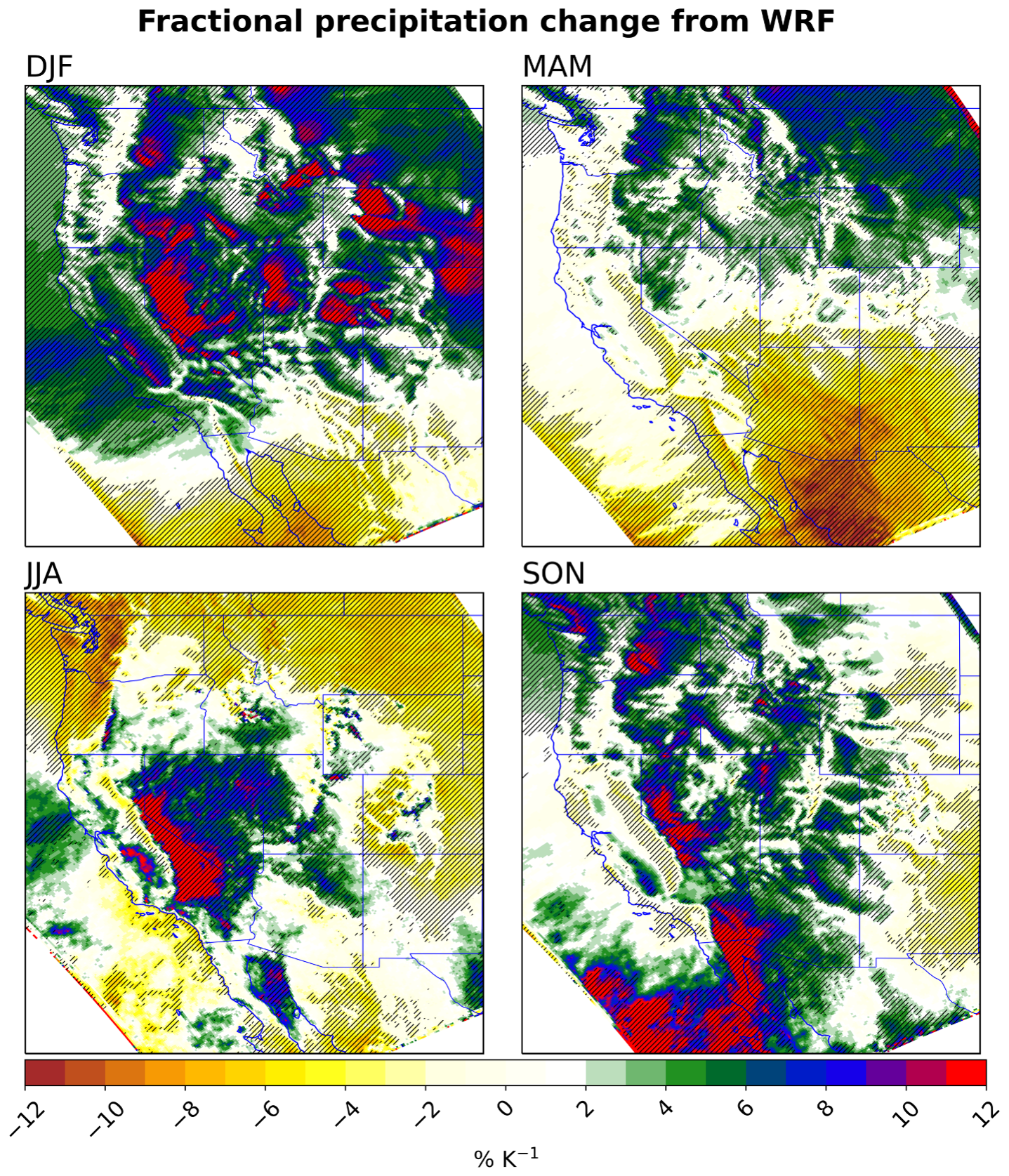
Figure 8 The mean future changes of the 16 GCMs in dynamically downscaled fractional precipitation normalized by the amount of global warming [% K⁻¹]. Hatching indicates statistical significance to the 95 % confidence interval when grid point distributions are subjected to a two-sided Student's t test. Stippling is not included for temperature because every grid point returns a p value smaller than 0.05.

4.2 Changes in extremes

The future fractional change in extreme (rx1day) precipitation is much more consistent across the WUS than for the mean, with intensified extremes occurring over most of the domain in both the parent and dynamically downscaled GCMs (Fig. 9, left column; Fig. S10 for individual GCMs). These changes in rx1day vary from roughly 0 % K⁻¹–12 % K⁻¹ across the domain in the downscaled ensemble mean. In both the GCM and downscaling cases, the spatial variations in the changes in rx1day can be traced in part to vertical velocity (defined by the pressure velocity) changes: spatial correlations of −0.7 (−0.3) are found between rx1day precipitation and vertical velocity changes in GCM (downscaling) experiments. Here, a negative correlation coefficient implies a positive relationship between upward vertical velocities and positive rx1day changes. However, the patterns of vertical velocity change are very different in the two cases. In the downscaling experiments, the largest intensification of rx1day occurs via upward vertical velocity increases on the lee side of latitudinally oriented mountain chains that are not resolved in the parent GCMs (Fig. 9 right column). Over large parts of these areas, the increases are super-Clausius–Clapeyron (> 7 % K⁻¹). This indicates that extreme precipitation intensifies at a greater rate than saturation specific humidity, commonly termed the thermodynamic component of extreme-precipitation scaling. Thus, WRF simulates greater dynamical intensification of extreme precipitation (e.g., Norris et al., 2019) than the GCMs and in a distinct topographically modulated pattern.

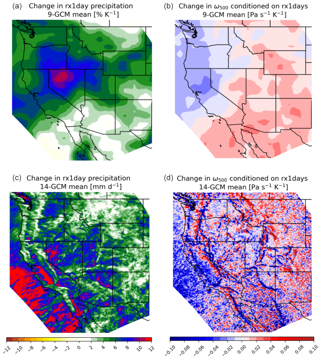
Figure 9 Future response in (a, c) rx1day precipitation [% K⁻¹] and (b, d) 500 hPa pressure velocity [Pa s⁻¹ K⁻¹] conditioned on rx1day occurrence for the (a, b) GCM and (c, d) WRF ensembles per degree of global warming [% K⁻¹]. Due to the lack of GCM data with daily vertical velocity outputs, we use a 14-GCM (9-GCM) mean for rx1day (pressure velocity); the WRF patterns of rx1day generally are similar for a 9-GCM mean (Fig. S11).

Next, we examine future changes in extreme heat, defined by the number of days exceeding the 99th percentile of the historical daily maximum surface air temperature (Tmax99). Consistent with extreme precipitation, these changes are normalized by global warming to account for the large intermodel spread in climate sensitivity (Fig. 10, left). Averaged across the WUS, Tmax99 exceedances increase by 11.9 ± 2.1 d yr⁻¹ K⁻¹. California, Oregon, and Washington see increases of 4–7 d yr⁻¹ K⁻¹, with coastal areas seeing increases of less than 5 d yr⁻¹ K⁻¹. The power of dynamical downscaling is particularly evident, as the GCMs (Fig. 10, top row) cannot simulate (i) the correct coastline geometry, leading to an unphysical intrusion of maximized ocean-influenced Tmax99 exceedances and (ii) the complex terrain of the WUS, which strongly modulates the snow coverage and subsequently the land surface sensitivity to warming. Additional examination reveals that the GCMs with the greatest regional mean warming are not necessarily the GCMs with the largest increase in exceedances (Figs. S5, S12). This discrepancy may be due to GCM differences in the simulation of synoptic-scale events that produce heat waves. Anthropogenic changes in such events may occur independently of mean temperature shifts (Fig. 7).

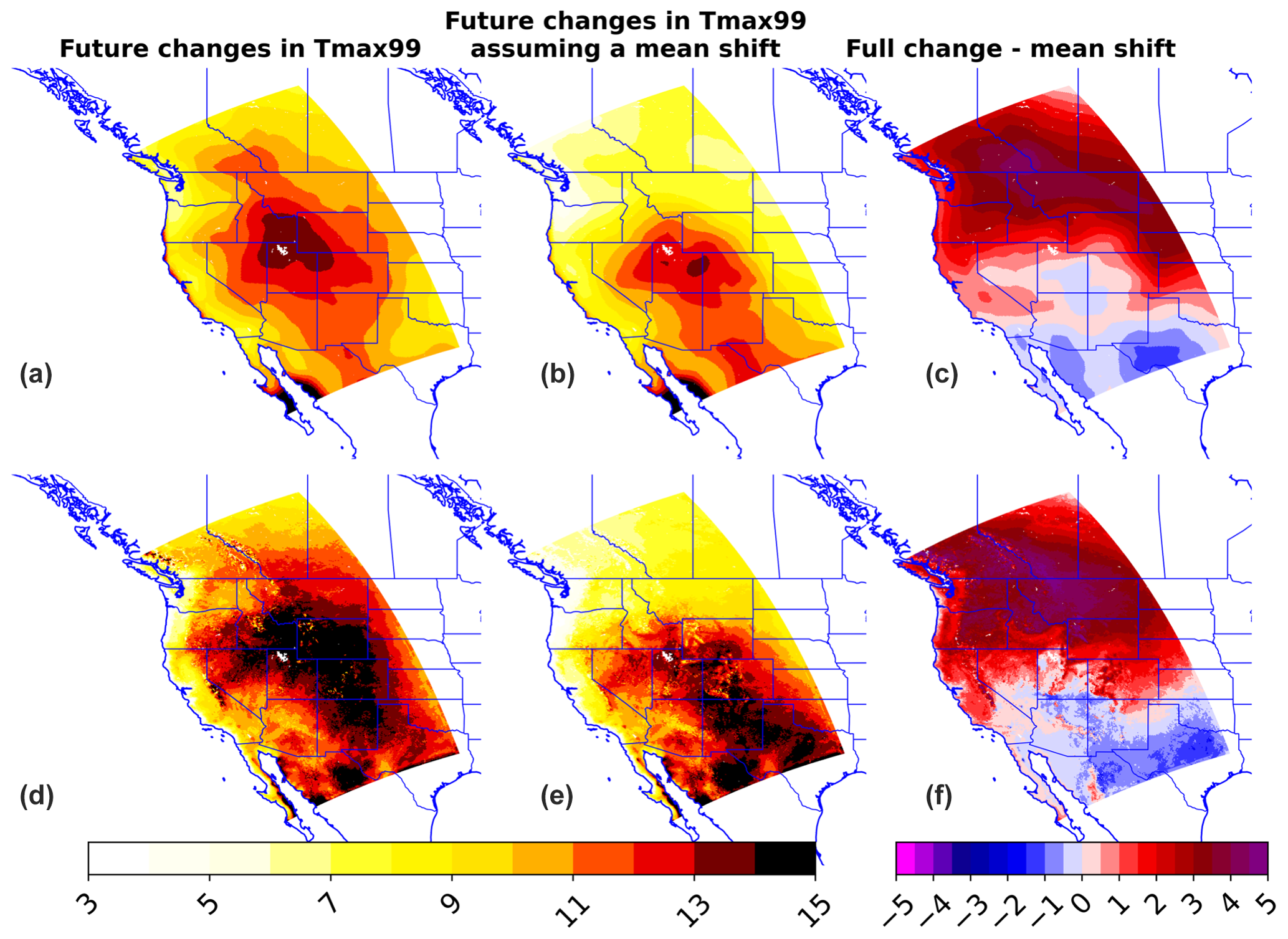
Figure 10 Future changes in the 99th percentile of surface daily maximum air temperature (Tmax99) per degree of global warming [d yr⁻¹ K⁻¹] considering the full change (a, d) and assuming a mean shift in the temperature distribution (b, e) for (a, b, c) GCMs and (d, e, f) WRF GCMs. The right panel presents the difference between the left and center panels. Parent GCM (WRF GCM) calculations utilize an 11-member (16-member) ensemble. When using the same 11-member ensemble, the WRF panels look similar (Fig. S13).

Next, we explore whether changes in Tmax99 exceedances are explainable by mean shifts in the temperature distribution. As shown in Fig. 10 (right column), the number of actual future Tmax99 exceedances from parent and dynamically downscaled GCMs can be quite different compared to the case where all quantiles in the temperature distribution are shifted equally based on the amount of local mean warming in Tmax99 (Fig. 10, middle column). Red (blue) pixels indicate regions where the tails of the temperature distribution are warming more (less) than can be explained by mean warming in Tmax99. Assuming a mean shift in Tmax99 significantly underpredicts the increase in exceedances by 3–4 d yr⁻¹ K⁻¹ across portions of California, Oregon, and Washington. Still greater underpredictions of future exceedances assuming a mean shift are seen across western Montana, Idaho, and portions of western Wyoming, particularly at higher elevations. Further south, however, the number of exceedances in Tmax99 can be explained mostly by mean shifts in Tmax99. Assuming a mean shift, exceedances are slightly overpredicted across portions of New Mexico and western Texas relative to GCM and WRF simulations. This analysis highlights that the intensification of extreme temperature events may not be entirely explainable by mean shifts in the temperature distribution alone, and parent and downscaled GCMs are broadly similar in this respect. However, there is also significant spatial structure in the downscaling patterns not seen in the GCMs, indicating that local atmospheric dynamics and local land–atmosphere feedbacks play a role in shaping change in the right tail of the temperature distribution.

5 Summary and conclusions

Future regional climate change remains difficult to project, given the low resolution of GCMs, particularly over a region of complex terrain such as the western US. In this study, we present a dataset containing 16 CMIP6 models dynamically downscaled with WRF over the region from 1980 to 2100 at 9 km grid spacing: the Western US Dynamically Downscaled Dataset (WUS-D3). The future projections are primarily based on the SSP3-7.0 high-emissions scenario, but we include two additional downscaled experiments with CESM2 of the SSP2-4.5 and SSP5-8.5 scenarios. An extensive evaluation of CMIP6 models' historical simulations over the western US has been conducted (Krantz et al., 2021; Goldenson et al., 2023) to identify the most suitable candidates for downscaling over this region. However, GCM selection was also based on the availability of data required to provide initial and boundary conditions to WRF. The optimal configuration of WRF over the western US was established via an extensive evaluation of an ERA5-driven WRF run (Rahimi et al., 2022). Numerous other challenges of using the CMIP6 data to force WRF are outlined in the methods.

Aside from the obvious improved representation of spatial patterns of meteorological variables, there are many notable improvements of the downscaling over raw GCMs when compared to observations over the historical period. For example, the WRF simulations largely correct for major wet biases (∼ 100 %) in the raw GCMs over Nevada, Wyoming, Montana, and Colorado. These bias reductions apply to both winter and summer, depending on the state. Moreover, the GCMs completely fail to represent the summertime precipitation maximum over Arizona and New Mexico, which is corrected in the downscaled experiments, albeit with some large wet biases therein. The WRF simulations also correct large summertime warm biases over much of the domain, particularly the interior states, due to the improved representation of terrain and resulting snowpack improvements. Finally, extreme precipitation (measured by rx1day) is greatly increased (generally about doubled) from the GCM values. In some cases, this amounts to wet biases from WRF, according to PRISM, but these apparent biases are mostly at high elevations where observational uncertainties are maximized (Lundquist et al., 2019).

There are, however, extensive and systematic biases that remain from the parent GCMs and in some cases are exacerbated. For example, the GCMs generally overestimate winter precipitation along the west coast, which likely results from unrealistically high moisture contained within atmospheric rivers (Norris et al., 2021) and other GCM biases transmitted to WRF. In the WRF simulations, these wet biases are amplified, likely as excessive moisture is forced up steeper orographic gradients than in the GCMs. Also, unlike the GCMs, the downscaled experiments are generally too cold compared to PRISM, particularly in winter, with some states exhibiting as much as a 5 K bias. These results are comparable to Rastogi et al. (2022), who used a different regional climate model, implying that inherited GCM biases may be to blame. The dynamical downscaling community should be frank about such biases, particularly in lieu of the fact that these biases are often artificially removed post-downscaling using bias correction. This practice is ubiquitous in hydrology and demand forecast modeling, as well as in statistical downscaling. Users of WUS-D3 should be open-eyed and wary about the possibility that these large historical biases may compromise the trustworthiness of its climate change signals.

The future downscaled climate change signals are shaped in physically credible ways by the regional model's more realistic coastlines and topography. Large-scale warming patterns are generally preserved from the parent GCMs but with enhanced warming adjacent to high terrain during winter and spring and over high elevations during summer. This locally enhanced warming occurs where relative snow losses are maximized in the future, a feature that cannot be captured at the GCMs' coarse resolution. Meanwhile, precipitation patterns undergo much greater transformation with downscaling. Although WRF preserves the broad pattern of subtropical drying and midlatitude wetting, WRF simulates additional local precipitation changes. In particular, mean precipitation changes are often consistent with wetting on the windward side of mountain complexes, as warmer, moister air masses are uplifted orographically during precipitation events, similar to Huang et al. (2020). There are large fractional precipitation increases on the lee side of mountain complexes, consistent with the theoretical work of Siler and Roe (2014). This could lead to significant changes in water resources and ecology across these arid landscapes. The intensification of precipitation and temperature extremes is also modified in significant ways by dynamical downscaling. Over complex terrain, precipitation extremes scale at much greater rates, on the order of 12 % K⁻¹. This greater scaling in WRF is likely due to greater dynamical enhancement of extreme precipitation over mountain ranges, as evidenced by the intensification of upward vertical velocity changes conditioned on extremes. Temperature extremes also intensify, as measured by future exceedances of historical 99th-percentile surface air temperature per degree of global warming. These are on the order of +5 d yr⁻¹ K⁻¹ along the west coast and approaching 15 d yr⁻¹ K⁻¹ in the interior west. The simulated changes are mostly greater than that predicted by a simple mean shift in the temperature distribution, indicating the effect of an extension of the right tail. The imprint of topography is evident in this change in the temperature distribution's shape, indicating the importance of local atmospheric dynamics and land surface feedbacks.

Despite the care taken in creating WUS-D3, this paper provides a forum to scrutinize the dynamical downscaling technique. For instance, here we assume that the ocean–atmosphere coupling is adequately preserved in downscaling since SSTs are prescribed to update regularly, and large-scale winds and temperatures are preserved in downscaling via spectral nudging. But is this a good assumption given that half of our 45 km grid covers the open Pacific, and so should a version of WRF with coupled ocean capabilities be used in future downscaling across the region? Also, as discussed previously, unrealistically large surface air temperature and precipitation biases in the parent GCMs were in some cases replaced by equally egregious biases in the downscaled solution. Despite a careful GCM selection process employed in this study, does this result motivate the consideration of a pre-downscaling bias correction procedure of GCM fields in future studies?

WUS-D3 constitutes the first comprehensive dataset of landscape-resolving climate projections over the western US. Although only temperature and precipitation projections have been evaluated here, the dataset includes all 2-D and 3-D meteorological and land surface variables at 6-hourly intervals with an auxiliary datastream of more than 20 land surface variables needed to drive downstream models (e.g., hydrology) offline. Thus, it represents a unique opportunity to explore potential future changes to a wide diversity of weather and climate phenomena over the region. These include but are not limited to atmospheric rivers, the North American monsoon, summer convective storms, intense heat waves, wildfire-related downslope winds, and ventilation by sea breezes. Moreover, these data may be used to drive offline and calibrated hydrology and fire-weather models to obtain more detailed projections of water resources and flooding and wildfire. Nevertheless, there are biases in the downscaled simulations, briefly documented here, which should be understood and appreciated when using the data for future projections. We strongly encourage the community to use these results with other dynamically and statistically downscaled products to develop risk assessments and bound uncertainty. Such intercomparisons of different downscaled products are critical to assessing a product's usefulness and applicability. Finally, for the express purpose of dynamical downscaling, we implore the CMIP7 protocol development team to mandate that new GCM outputs for ta, ua, va, and hus be reported on 20–30 isobaric pressure levels and at 6-hourly intervals (along with ps), as increasingly powerful computing platforms are beginning to enable the community to consider dynamically downscaling large ensembles of GCMs.