the Creative Commons Attribution 4.0 License.
the Creative Commons Attribution 4.0 License.
 | 15 Mar 2024
Validation of a new global irrigation scheme in the land surface model ORCHIDEE v2.2
Pedro Felipe Arboleda-Obando
Agnès Ducharne
Philippe Ciais
Irrigation activities are important for sustaining food production and account for 70 % of total global water withdrawals. In addition, due to increased evapotranspiration (ET) and changes in the leaf area index (LAI), these activities have an impact on hydrology and climate. In this paper, we present a new irrigation scheme within the land surface model ORCHIDEE (ORganising Carbon and Hydrology in Dynamic EcosystEms)). It restrains actual irrigation according to available freshwater by including a simple environmental limit and using allocation rules that depend on local infrastructure. We perform a simple sensitivity analysis and parameter tuning to set the parameter values and match the observed irrigation amounts against reported values, assuming uniform parameter values over land. Our scheme matches irrigation withdrawals amounts at global scale, but we identify some areas in India, China, and the USA (some of the most intensively irrigated regions worldwide), where irrigation is underestimated. In all irrigated areas, the scheme reduces the negative bias of ET. It also exacerbates the positive bias of the leaf area index (LAI), except for the very intensively irrigated areas, where irrigation reduces a negative LAI bias. The increase in the ET decreases river discharge values, in some cases significantly, although this does not necessarily lead to a better representation of discharge dynamics. Irrigation, however, does not have a large impact on the simulated total water storage anomalies (TWSAs) and its trends. This may be partly explained by the absence of nonrenewable groundwater use, and its inclusion could increase irrigation estimates in arid and semiarid regions by increasing the supply. Correlation of irrigation biases with landscape descriptors suggests that the inclusion of irrigated rice and dam management could improve the irrigation estimates as well. Regardless of this complexity, our results show that the new irrigation scheme helps simulate acceptable land surface conditions and fluxes in irrigated areas, which is important to explore the joint evolution of climate, water resources, and irrigation activities.
- Article
(6922 KB) - Full-text XML
-
Supplement
(4527 KB) - BibTeX
- EndNote


Irrigation seeks to increase crop yields by reducing plant water stress (Siebert and Döll, 2010; Klein Goldewijk et al., 2017) and supports about 43 % of the world's food production on about 20 % of the arable land (Siebert and Döll, 2010; Grafton et al., 2017). The beneficial effects of irrigation on food production, population, and economic growth have dramatically pushed the increase in irrigated areas during the 20th century from 28 Mha in 1850 to 276 Mha in 2000 (Klein Goldewijk et al., 2017; Siebert et al., 2015). As a consequence, by the year 2000, irrigation accounted for 70 % of the total water withdrawn (between 2657 and 3594 km3 yr−1). The consumptive water use, i.e., the part of the withdrawn water that actually becomes evapotranspiration (ET) and does not flow to surface supplies and groundwater, represents half of that volume (between 1021–1598 km3 yr−1, which is around 1.7 % of total continental ET of 75.6×10³ km3 yr−1, according to Jung et al., 2019) and represents around 90 % of the total consumptive water use by human activities (Pokhrel et al., 2016; Döll et al., 2012; Hoogeveen et al., 2015).
Water abstraction and corresponding ET increase have a direct impact on the water and energy balances and on surface and subsurface hydrology (Döll et al., 2012; Taylor et al., 2013; Vicente‐Serrano et al., 2019). The atmosphere also reacts to these changes in land surface fluxes, for instance, with regional increases or decreases in rainfall rate or decreases in temperature extremes (Lo and Famiglietti, 2013; Guimberteau et al., 2012b; Cook et al., 2015; Al-Yaari et al., 2019; Thiery et al., 2020). Thus, it was recently shown that climate models better capture historical trends in evapotranspiration if they account for irrigation and its expansion, although the resulting cooling effect is too strong if irrigation is not limited by water availability (Al‐Yaari et al., 2022). Finally, with the acceleration of climate change, the irrigation water demand is likely to increase, not only by expansion of the irrigated area but also by increasing temperature and changing precipitation variability (Wada et al., 2013). All of these impacts and effects have promoted the inclusion of irrigation inside land surface models (LSMs), which represent the continental branch of the hydrologic cycle in the Earth system models (Pokhrel et al., 2016).
Besides LSMs, global hydrology models (GHMs) also represent irrigation at a global scale. Originally, GHMs were developed to assess water resource availability and water use. In GHMs, irrigation demand is equal to the increase in the ET due to irrigation (i.e., water that becomes evapotranspiration). This ET increase is estimated as the differences between crop-specific potential ET and actual ET with no irrigation (Siebert and Döll, 2010; Mekonnen and Hoekstra, 2011; Wada and Bierkens, 2014; Chiarelli et al., 2020). Following Allen et al. (2006), the crop-specific potential ET is defined as , where parameter kc depends on the crop type and growing stage, and ET0 is the reference crop ET, corresponding to the atmospheric evaporative demand. Some models also consider conveyance losses and return flows to rivers and aquifers; i.e., they consider the total water withdrawal (water demand plus losses), using empirical ratios of irrigation efficiency (ratio of ET increase to water withdrawal) or specific rules according to the irrigation technique (Rost et al., 2008; Jägermeyr et al., 2015). The advantage of calculating the withdrawn volume is that it allows comparison and validation with datasets of reported values, for example, the Food and Agriculture Organization (FAO) AQUASTAT dataset (Frenken and Gillet, 2012). GHMs explicitly represent water supply sources (Döll et al., 2012) and allow the estimation of non-sustainable groundwater used for irrigation (Wada et al., 2012). Some GHMs also simulate water allocation (use of water by type of source), based on rules that use information of local infrastructure and environmental flow estimations (Siebert et al., 2010; Hanasaki et al., 2008a).
LSMs do not generally use potential evapotranspiration (PET) to estimate irrigation demand. The reason is that LSMs do not deduce ET from daily PET input data but from the surface energy balance at hourly and subhourly time steps. This difference raises consistency issues between empirical PET formulas and potential ET rates in LSMs (Barella-Ortiz et al., 2013). Some LSMs prescribe irrigation rates estimated offline (Lo and Famiglietti, 2013; Cook et al., 2015), but most of the LSMs and some GHMs estimate irrigation demand by calculating a deficit such as a soil moisture deficit between actual and a target soil moisture (Haddeland et al., 2006; Hanasaki et al., 2008a; Leng et al., 2014; Pokhrel et al., 2015; Jägermeyr et al., 2015). Some LSMs, which benefit from a physically based description of surface runoff and drainage, can explicitly calculate return flow, but conveyance losses are not explicitly included (Yin et al., 2020; Leng et al., 2017). In addition, irrigation shortage due to water availability is not always well represented in those LSMs (and GHMs) that include this feature, as some of them include a virtual infinite reservoir to fulfill irrigation demand (Ozdogan et al., 2010; Leng et al., 2014; Pokhrel et al., 2012). This virtual reservoir may represent fossil groundwater use and water table depletion, which is important in some areas like the High Plains (in the USA) and India (Pokhrel et al., 2015; Leng et al., 2017; Felfelani et al., 2021). Water allocation is commonly based on a stream water supply first rule (Guimberteau et al., 2012b), with some exceptions that use the global groundwater inventory from Siebert et al. (2010) (Leng et al., 2017; Felfelani et al., 2021). These rather simple irrigation schemes are used in land surface–atmosphere simulations to assess irrigation effects on climate (Puma and Cook, 2010; Lo and Famiglietti, 2013; Guimberteau et al., 2012b; Lo et al., 2021) but not on water resources assessment.
ORCHIDEE (ORganising Carbon and Hydrology in Dynamic EcosystEms), the LSM of the IPSL (Institut Pierre-Simon Laplace) Earth system model (Krinner et al., 2005; Boucher et al., 2020), has been used to assess irrigation effects on climate. First attempts to crudely represent irrigation were based on potential evaporation and potential transpiration for a generic crop type (de Rosnay et al., 2003; Guimberteau et al., 2012b). This irrigation scheme restrains irrigation according to available water and includes simple allocation rules. Recently, ORCHIDEE-CROP, a version of the model that includes a crop phenology module, improved the irrigation scheme by representing flood and paddy irrigation techniques and was tested in an offline mode in China (Yin et al., 2020). These improvements open the possibility for assessing irrigation effects on water resources. This is important, as there is evidence that some modeling biases within ORCHIDEE in offline and coupled modes are correlated to the surface equipped for irrigation (Mizuochi et al., 2021).
Here, we present evidence on the effect of irrigation on the reduction in the modeling biases in some key variables, like ET and leaf area index (LAI), and on river discharge and total water storage anomalies (TWSAs). After describing the ORCHIDEE model and the global irrigation scheme, we set the parameter values using short simulations. We perform a sensitivity analysis and a simple parameter tuning to fit observed irrigation rates. We then perform long simulations, and we compare irrigation estimates to observations and corresponding variability due to parameter values and input maps. We validate irrigation estimates by reported values, and we assess the spatial variability in the modeling bias. Then we assess the modeling bias against observed datasets using a factor analysis, with and without irrigation, for ET and LAI. In large basins with extensive irrigation activities, we compare simulated and observed values of discharge and total water storage anomalies (TWSAs). We also show some results on the correlation between the irrigation bias and some landscape descriptors as a first step to improve the realism of the scheme. Finally, we discuss the results, and we present the main conclusions and perspectives.
2.1 ORCHIDEE v2.2
ORCHIDEE describes the fluxes of mass, momentum, and heat between the surface and the atmosphere (Krinner et al., 2005). Here we use version 2.2, which is close to the version used for CMIP6 (corresponding to 2.0). Version 2.0 has been described in many papers (Cheruy et al., 2020; Boucher et al., 2020; Tafasca et al., 2020), and version 2.2 only adds a few minor bug corrections. We summarize the main characteristics of the model that mediate in the simulation of irrigation.
In each grid cell, vegetation is represented by a mosaic of up to 15 plant functional types (PFTs), including generic C3 and C4 crops, as well as generic C4 grasses, and tropical, boreal, and temperate C3 grasses. The PFTs fractions are described by the LUHv2 dataset (Lurton et al., 2020), and each PFT is characterized by a specific set of parameters applied to the same set of equations (Boucher et al., 2020; Mizuochi et al., 2021). Plant phenology is controlled by the STOMATE module, which couples photosynthesis and the carbon cycle and computes the evolution of the leaf area index (LAI), and all of these processes depend on the CO2 atmospheric concentration (Krinner et al., 2005).
A specialized version of ORCHIDEE has been proposed by Wu et al. (2016) and evaluated by Müller et al. (2017) to better describe temperate crops, with phenology thresholds based on accumulated degree days after the sowing date, improved carbon allocation to reconcile the calculations for leaf and root biomass and grain yield, and nitrogen limitation related to fertilization. It was not used in this work owing to a lack of ubiquitous parameters at the global scale, so C3 and C4 crops are simply assumed to have the same phenology as natural grasslands but with higher carboxylation rates and adapted maximum possible LAI (Krinner et al., 2005). The crop growing season depends on mean annual air temperature, as detailed in Krinner et al. (2005). In cool regions, it starts after a predefined number of growing degree days, while in warm regions, it starts a predefined number of days after soil moisture has reached its minimum during the dry season. In intermediate zones, the two criteria have to be fulfilled. The end of the growing season also depends on temperature and water stress and on leaf age.
Roots constitute an important link between the carbon and the water balance. In each PFT, root density decreases exponentially with depth, and the parameter that controls the decay is PFT-dependent. It is worth noting that the root density profile is constant in time and goes down to the bottom of the soil column, set at 2 m, but forest PFTs have much denser roots than crop and grass PFTs, especially in the bottom part of the soil (Wang et al., 2018). The resulting root density profile is combined with the soil moisture profile and a water stress function to define the water stress factor of each PFT on transpiration (Tafasca et al., 2020) and to estimate the water uptake for transpiration (de Rosnay et al., 2002).
Evapotranspiration is represented by a classical aerodynamic approach and is composed of snow sublimation, interception loss, bare soil evaporation (E), and transpiration (T). The first two proceed at a potential rate, while bare soil evaporation is limited by the upward diffusion of water through the soil, and transpiration is controlled by a stomatal resistance, which depends on soil moisture and vegetation parameters. The vegetation types are grouped into three soil columns according to their physiological behavior: high vegetation (eight forest PFTs); low vegetation (six PFTs for grasses and crops); and bare soil. While the energy balance is calculated for the whole grid cell (Boucher et al., 2020), a separate water budget is calculated independently for each soil column in order to prevent forest PFTs from depriving the other PFTs of soil moisture.
Vertical soil water flow is represented by a 1-D Richards equation coupled to a mass balance, and lateral flow between cells and soil columns is neglected (de Rosnay et al., 2002; Campoy et al., 2013). Here, soil depth is set at 2 m and discretized into 22 layers to finely model the lower layers implicated in drainage. Infiltration is simulated as a sharp wetting front, based on the Green and Ampt model (Tafasca et al., 2020; D'Orgeval et al., 2008). The resulting increase in top soil moisture is redistributed by the Richards equation. The bottom boundary condition assumes free drainage, equal to the hydraulic conductivity of the deepest node. The saturated hydraulic conductivity decreases with depth, but roots increase the hydraulic conductivity near the surface (D'Orgeval et al., 2008). Soil parameters are a function of soil texture (Tafasca et al., 2020), and the spatial distribution is taken from the Zobler (1986) map.
A routing scheme transfers surface runoff and drainage from land to the ocean through a cascade of linear reservoirs (Ngo-Duc et al., 2007; Guimberteau et al., 2012a). Each grid cell is split into subbasins, according to a 0.5° flow direction map. Three reservoirs are considered inside every subbasin, representing groundwater, overland, and river reservoir, and each one presents a distinct residence time (Ngo-Duc et al., 2007). The groundwater reservoir collects drainage from the soil column, while the overland reservoir collects surface runoff. Both reservoirs are internal to each subbasin and flow to the stream reservoir, which also collects streamflow from the upstream basins and contributes to large-scale routing across subbasins and grid cells. Note that there are two surface reservoirs, overland representing the headwater streams, and a river reservoir representing large rivers.
The water and energy budgets and the routing scheme are computed at the same 30 min time step, while the carbon and plant phenology processes in STOMATE are solved with a daily time step.
2.2 Irrigation scheme
The irrigation scheme (Fig. 1) is based on the flood irrigation representation from Yin et al. (2020), but it includes some changes in the parameterization to run at a global scale. The flood irrigation technique (which consists of adding water to the soil surface to achieve a certain soil moisture content) is chosen for global simulations, as it is the most used technique (Jägermeyr et al., 2015; Sacks et al., 2009).
First, the scheme defines a root zone depth in the crop and grass soil column, based on the cumulative root density (CRD), ranging from 0 at the soil surface to 1 at the soil bottom; the root zone comprises all soil layers with a CRD below a user-defined threshold, Rootlim. When the threshold is set to 0.9, the root zone includes 90 % of the root system. For a 2 m soil column with 22 layers, and an exponential root density decay of 4 (default value for crops and grasses in ORCHIDEE), this threshold defines a root zone depth of 0.65 m, encompassing 11 soil layers.
We can then define a soil moisture deficit D (mm) in the root zone as the sum of the difference between actual soil moisture and a soil moisture target in all layers of the root zone, as follows:
where Wi and (both in mm) are the actual and field capacity soil moisture in soil layer i, respectively, and β is a user-dependent parameter that controls the target value with respect to field capacity (shown in Fig. S10 with soil texture). When soil moisture drops below the target, irrigation is triggered. To prevent irrigation when there is no plant development, for example, during winter, we set the deficit D to zero if all crops and grasses are below a certain LAI threshold, LAIlim. By doing so, we overlook irrigation used to enhance germination and tend to underestimate irrigation amounts.
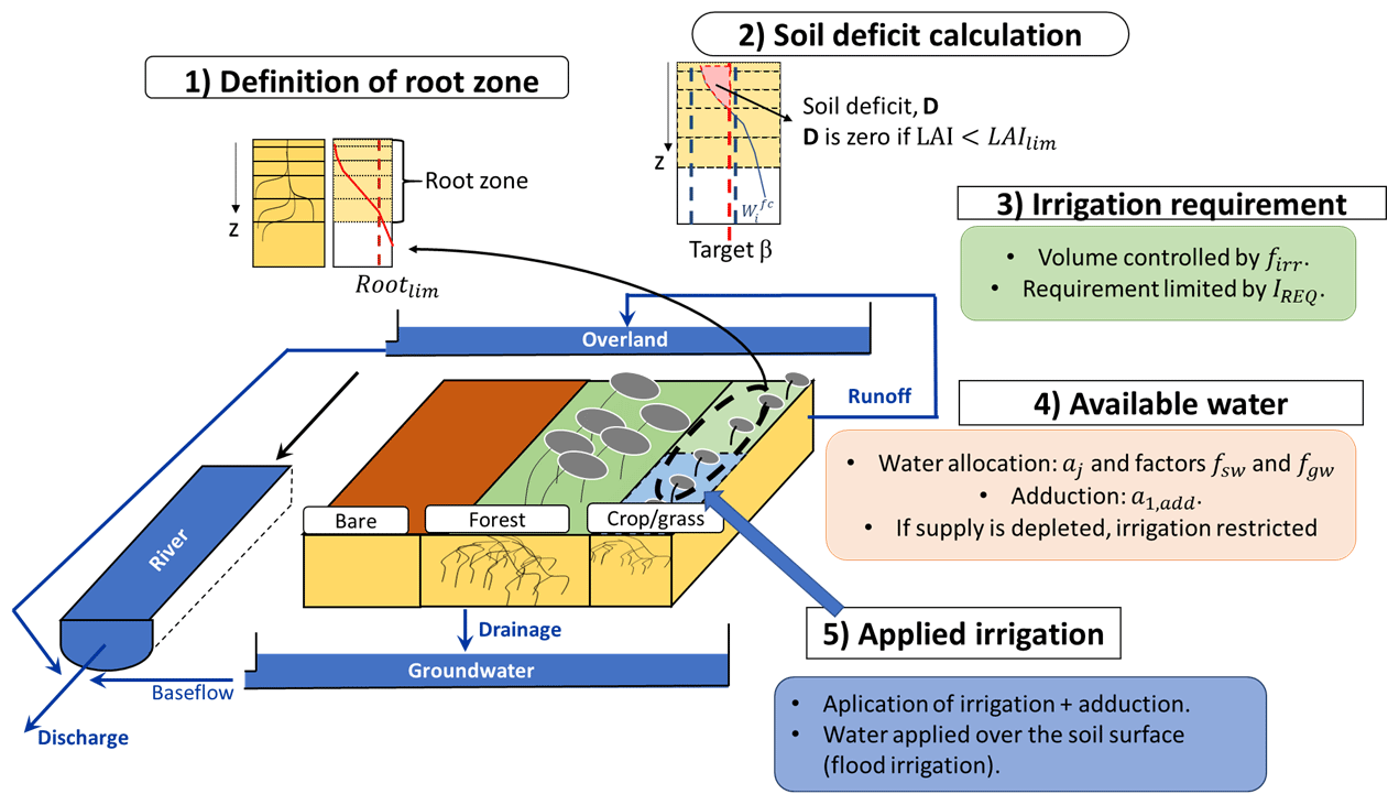
Figure 1ORCHIDEE model and new irrigation scheme. See the text for an explanation of the parameters.
The irrigation requirement Ireq (mm s−1) is calculated as
where firr is the fraction of irrigated surface (–) in the grid cell, defined by a map of irrigated fractions. The map that prescribes the irrigated fraction may change every year, but note that we do not separate the irrigated area into a separate soil column; i.e., the soil column includes crops (both irrigated and rainfed) and grasses. Imax is a user-defined maximum hourly irrigation rate (mm h−1). This third threshold is used to avoid excessive runoff production when the deficit is larger than the infiltration capacity of the soil. Therefore, the deficit is fulfilled progressively over the subsequent time step. The effective irrigation (I; see below) is uniformly applied over the crop and grass soil column. Therefore, care must be taken by the model that the irrigated fraction is not greater than the soil column. If the fraction of the irrigated surface is much smaller than the crop and grass soil column, then irrigation will eventually be spread over a larger area than the actual irrigated surface. This particular case (an important difference between irrigated fraction and soil column fraction) could likely result in an overestimation of the amount of irrigation (mainly because the water put on the surface will not be sufficient to reach the soil moisture target; see Fig. S9). Besides, the fraction of irrigation water that actually evaporates could be larger than in reality. The latter could lead to an overestimation of the evapotranspiration increase, especially in areas that are energy-controlled (Puma and Cook, 2010), and an overestimation of irrigation efficiency.
Irrigation can be withdrawn from three routing reservoirs, but the effective water availability, Aw (mm), also depends on the facility to access surface water and groundwater, and it can be reduced to preserve environmental flows as follows:
In this equation, Sj (mm) is the volume storage in each routing reservoir, with index j equal to 1, 2, and 3 for the stream, overland, and renewable groundwater (i.e., shallow aquifers that are recharged by drainage at the soil bottom) reservoirs, respectively. To prevent the complete depletion of these reservoirs, which all feed streamflow and support aquatic ecosystems, we mimic an environmental flow regulation by reducing the available volume, owing to a user-defined parameter aj, to between 0 and 1. It is set here at 0.9 for all three reservoirs, so as to keep at least 10 % of the available water at each time step. The facility to irrigate from surface water reservoirs (S1 and S2) and groundwater reservoir (S3) is accounted for by factors fsw and fgw, also ranging between 0 if the reservoirs cannot be used and 1 if they are fully accessible. In the present application, these factors represent the fraction of irrigated areas that are equipped for irrigation with surface and groundwater, respectively, following the global map of Siebert et al. (2010). We do not consider irrigation from nonconventional sources (e.g., wastewater and water from desalination plants). This map assumes that a grid cell is either equipped for groundwater irrigation or for surface water irrigation, so .
Eventually, the actual irrigation I (mm s−1) is estimated at each time step by comparing Ireq, i.e., the demand, to water availability Aw (mm), i.e., the supply, as follows:
If we assumed that water abstraction Qj from each natural reservoir due to irrigation withdrawal is simply proportional to the available water in each of them, then it would be given by the following equations, with the sum of the three right-hand side terms being equal to I:
But we chose to implement an additional constraint for surface water withdrawals, which are withdrawn from the stream reservoir (corresponding to large rivers) at a higher priority. This new constraint leads to the definition of the revised set of equations, where the total surface water availability is . as follows:
The sum of Q1, Q2, and Q3 still equals I.
When , i.e., there is a deficit and the water supply cannot satisfy the irrigation demand, then the scheme may adduct water from the neighboring grid cell with the largest streamflow volume. The choice of water adduction was introduced in Guimberteau et al. (2012b) but was disabled due to the coarse modeling resolution (grid cell larger than 100×100 km in size). Here we use a similar parameterization, but we add a user-defined parameter to take into account the facility to access distant river reservoirs:
In this equation, water adduction Q1,add from the largest river reservoir in the neighboring grid cell S1,add, will depend on the facility of access represented by the factor a1,add. This factor can range between 0 if there is no adduction and 1 if the distant river reservoir is fully accessible for water adduction.
The irrigation water, I+Q1,add, is finally added at the soil surface for infiltration, thus resembling a flood or drip irrigation technique. We note that irrigation is not restricted to an optimal period during the day but may be triggered at any moment. It may lead to an overestimation of evapotranspiration (Ozdogan et al., 2010). We do not represent dams operation in this simulation, even if they play an important role in modulating the temporal dynamics of surface water and ensure water supply for irrigation in many large river basins (Pokhrel et al., 2016; Hanasaki et al., 2008a).
3.1 Input data for ORCHIDEE
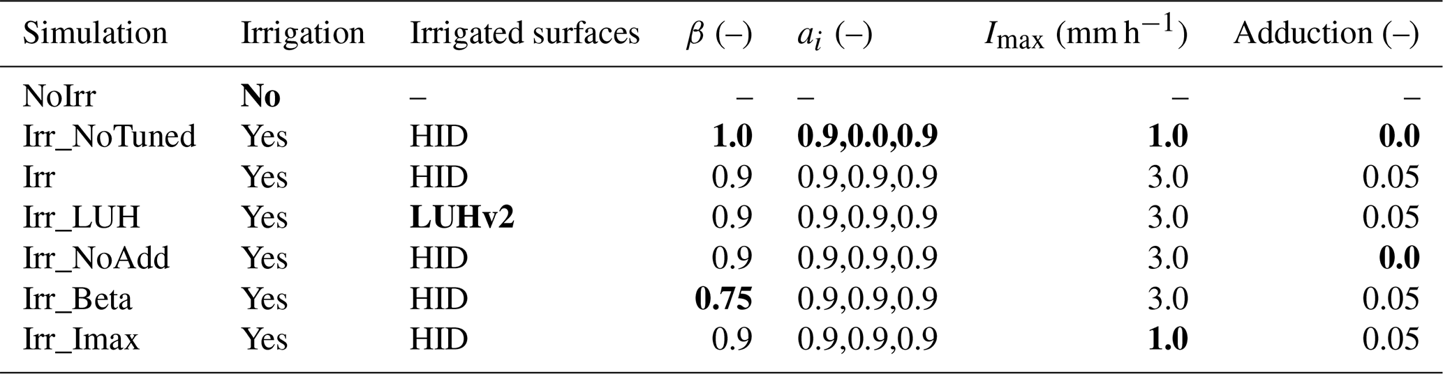
First, ORCHIDEE is run at global scale in offline mode. We run the model for the period 1970–2013, but we leave the first 10 years as warm-up, and we focus our analysis on the period 1980–2013. We use GSWP3 (van den Hurk et al., 2016) as meteorological forcing (http://hydro.iis.u-tokyo.ac.jp/GSWP3/, last access: 28 February 2024), with a resolution of 0.5°. We also run short simulations for the sensitivity analysis and parameter tuning (see Sect. 4). We prescribe the irrigated surfaces in transient mode; i.e., irrigated surfaces may change every year, based on the Historical Irrigation Dataset (HID) from Siebert et al. (2015) and on Land Use Harmonization 2 (LUHv2) dataset from Hurtt et al. (2020).
HID presents a map every 10 years before 1980 and every 5 years after at 5 arcmin resolution, and for each year, we use the nearest map in time to avoid data interpolation; LUHv2 presents a map every year with a 0.25° resolution. The main difference between the HID and LUHv2 maps is that HID prescribes the area that is equipped for irrigation (AEI), while LUHv2 prescribes the area that is actually irrigated (AAI). As a result, the HID dataset has a greater irrigated surface (3.0×10⁶ km2 for HID; 2.5×10⁶ km2 for LUHv2 at a global scale around the year 2000). It also means that AAI should be included in the AEI if the two datasets share a similar spatial distribution. But this is not the case, as the two datasets rely on different information sources that are processed with different methods (de Oliveira, 2022). The performed simulations use uniform parameters over irrigated areas, and the main changes between simulations are summarized in Table 1. As a reference, we use a simulation with no irrigation, called NoIrr, while simulation Irr, with irrigation activated, uses parameter values according to results from the sensitivity and tuning analysis (Sect. 4) and the HID maps. The simulation Irr_NoTuned also activates irrigation and uses the HID dataset as input, but it uses a priori parameter values. This latter simulation does not consider the conclusions from the sensitivity analysis and, for instance, does not activate irrigation withdrawal from the overland reservoir or adduction.
We run additional simulations to assess the uncertainty in the simulated irrigation amount and the influence of the most sensitive parameters, according to the sensitivity analysis. The impact of the deactivation of adduction in our scheme is considered in simulation Irr_NoAdd, the effects of changes in the β value are considered in simulations Irr_NoTuned, Irr, and Irr_Beta, and finally the effect of changes in the Imax value is considered in simulation Irr_Imax. All of these simulations use HID to prescribe irrigated areas. We analyze the effect of the large differences in prescribed irrigated areas on irrigation amounts using the LUHv2 dataset as input (simulation Irr_LUH) and using the same parameter values as the Irr simulation.
Table 1Simulations with inputs and parameter values. The units of the parameter are given in parentheses. The “–” symbol means that the parameter corresponds to a fraction and does not have a unit. The change in parameter values with respect to the Irr simulation is shown in bold typeface.
3.2 Validation datasets and landscape descriptors
The validation of the new irrigation scheme and its effect on the model bias is focused on five variables: evapotranspiration, leaf area index, discharge, irrigation withdrawal, and total water storage anomalies. We also use two landscape descriptors datasets (see below).
-
Irrigation water withdrawals. We use two datasets. First, we compare the simulated irrigation rates with values from the FAO AQUASTAT database (https://www.fao.org/aquastat/en/, last access: 28 February 2024) reported in Frenken and Gillet (2012) for irrigation volumes around the year 2000. AQUASTAT is based on reported values at the country scale, so it does not inform on seasonal values or their spatial distribution. In countries with a lack of information, data are completed using modeling outputs to estimate the plant requirement and country level ratios of irrigation efficiency to calculate the irrigation water withdrawal (Hoogeveen et al., 2015). While the plant requirement corresponds to the increase in the evapotranspiration, the irrigation water withdrawal is the volume that is abstracted from the natural reservoirs and includes the losses and return flows.
We also use the spatially explicit information of irrigation water withdrawal around the year 2000 from Sacks et al. (2009). This reconstruction uses national level census data, primarily from AQUASTAT, with maps of croplands by crop type, areas equipped for irrigation, and climatic water deficit. The result is a gridded map with a resolution of 0.5°.
-
Evapotranspiration. We use two datasets. The first product is GLEAM v3.3a, which combines satellite-observed values of soil moisture, vegetation optical depth, and snow water equivalent, reanalysis of air temperature and radiation, and a multisource precipitation product at 0.25° resolution (Martens et al., 2017). The second dataset is FLUXCOM (Jung et al., 2019), which merges Fluxnet eddy covariance towers with remote sensing (RS) and meteorological (METEO) data, using machine learning algorithms at 0.5° resolution. Here we use RS+METEO products, specifically the averages of RS+METEOWFDEI and RS+METEOCRUNCEP v8, to cover the analysis period.
-
Leaf area index. We use the LAI3g dataset (Zhu et al., 2013) climatological values for the period 1983–2015. This dataset applies a neural network algorithm on satellite observations of the normalized difference vegetation index (NDVI) 3g to estimate LAI at 5 arcmin resolution.
-
River discharge. We use monthly data from the Global Runoff Data Centre (GRDC; https://www.bafg.de/GRDC-/EN/Home/homepage_node.html, last access: 28 February 2024) in 14 large basins with strong irrigation activities. We choose the station nearest to the river mouth that also has data available for the study period (Fig. S4 shows the basins and its corresponding discharge station). Basin boundaries were delineated with the flow directions map used by ORCHIDEE (Sect. 2.1).
-
Total water storage anomalies. We compare the total water storage anomalies (TWSAs) from our simulations with three different monthly products of TWSAs, based on GRACE (Gravity Recovery and Climate Experiment) observations that are based on global mascon solutions that are suitable for hydrologic applications (Scanlon et al., 2016), including CSR (Save et al., 2016); GRC Tellus, hereafter called TELLUS (Watkins et al., 2015); and NASA GSFC (Loomis et al., 2019). CSR has a spatial resolution of 0.25°, while TELLUS and NASA GSFC have a resolution of 0.5°. As the differences between products at the large river basin scale are small, we use the average value of the three products. All of the products cover the period from April 2002 to the end of the simulation in 2014.
-
Landscape descriptors. We compare the simulation results with two landscape descriptors which are linked to irrigation and may contribute to the irrigation bias. We use the fraction of irrigated rice around the year 2000 from MIRCA2000 (Portmann et al., 2010a) (see the spatial distribution and focus on Southeast Asia in Fig. S5) and the location and volume of major dams based on the Global Reservoir and Dams database, GRanD (Lehner et al., 2011). GRanD contains information on the maximum storage capacity and main use of dams with reservoirs larger than 0.1 ha. Here we consider dams that have irrigation as their main purpose.
3.3 Data processing and analysis
We aggregate and interpolate all the observed data to the 0.5° spatial resolution of the ORCHIDEE simulations. For ET, we mask GLEAM and the simulated data according to FLUXCOM, which does not cover all the continents, so all the comparisons are made over the same grid cells with available information. For LAI, we exclude grid cells with no data in LAI3g from the analysis. We compare grid cell values and zonal average values. The statistical significance of the mean difference between observed and simulated time series is assessed with a Student's t test at the 5 % significance level.
We use the simulated discharge from the grid cell that best matches the watershed area upstream of the discharge station. In addition, we only use time steps with data available from observations so that both time series agree. For TWSAs, we compare observed and simulated basin averages. As ORCHIDEE gives the total water storage (TWS) value, we normalize the time series with the mean value of the NoIrr simulation for the period 2002–2008, which is the same as the observed products. In this way, the effect of irrigation over TWS is observed in the simulated time series.
In addition to direct comparison at the grid cell, zonal, or basin scale, we perform a factor analysis to reveal relationships between modeling bias and landscape descriptors. We use the fraction of irrigated areas around 2000 from HID, as well as the fraction of irrigated rice from MIRCA2000, both interpolated to the ORCHIDEE resolution. We categorized grid cells into six classes by irrigation fraction levels based on the two datasets, following Mizuochi et al. (2021): class 1 0 %; class 2 0 % to 5 %; class 3 5 % to 10 %; class 4 10 % to 20 %; class 5 20 % to 50 %; and class 6 50 % to 100 %.
We also performed a comparison between the average basin-scale irrigation bias and the volume capacity of dams used for irrigation within the basin, according to GRanD. We use Pearson's correlation coefficient (r) as a metric for the correlation analysis.
4.1 Sensitivity analysis
Short simulations were run to assess the sensitivity of the irrigation amount at the global scale to different parameter values, which are assumed to be uniform in all irrigated areas. We used GSWP3 as meteorological forcing and the LUHv2 from Hurtt et al. (2020) to prescribe the irrigated surfaces (see Sect. 3.1). We ran a total of 23 simulations with varying parameters, plus a reference simulation with no irrigation. All of them were run with the same initial conditions for 3 years (1998–2000), and a comparison of the irrigation amount and ET increase was performed for the year 2000. Using the last simulation year, we reduce the effect of the common initial conditions on the simulation results, and the year 2000 corresponds to the values given in AQUASTAT and Sacks et al. (2009). Note that we use a single meteorological forcing dataset and compare our estimates to a single set of observed AQUASTAT data for the period around the year 2000. We choose to compare our estimates for the year 2000 because this year is commonly used as the reference period in the literature concerning the estimation of the amount of irrigation on a global scale (see, e.g., Pokhrel et al., 2016; Table 2). The choice of the year 2000 is mainly due to the existence of more complete reported or observed values for that year, as well as simulated estimates. We use the same reference period to compare our results with independent data. A brief description of each parameter, as well as the unit, range, and values used in the sensitivity analysis, is shown in Table 2.
Table 2Parameters of the irrigation module, brief description, range, and values used in the sensitivity analysis. Values in bold correspond to the reference value. Note that, for parameter ai, the three reservoirs share the same value.
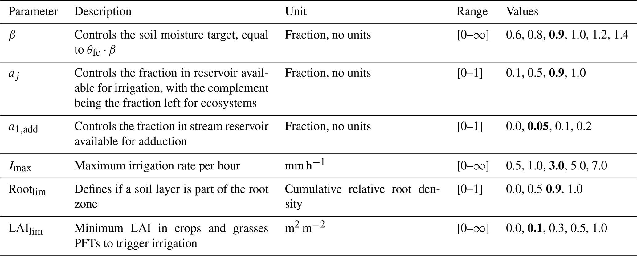
We change the value of one parameter at a time (one-at-a-time screening; see Mishra, 2009; Song et al., 2015), and then we observe its effect on the irrigation rate and on the increase in evapotranspiration. We tried to include the full range of parameters, but it is worth noting that in some cases, values were restricted to ensure an expected behavior. In the case of β, we set values around 1.0 (target equal to the field capacity soil moisture), as it seems a plausible target for flood irrigation, but note that values higher than 1.4 or lower than 0.6 are possible. Theoretically the upper limit is infinite, but values above 1.5 may exceed the saturated soil moisture for some soil textures, and the lower limit is zero (see Table S4). For adduction, we set parameter values under 0.2 (20 % of streamflow available for adduction at every time step), which seems high enough to represent water adduction in large river basins (Leng et al., 2015). In the case of the LAIlim and Imax, upper values were selected a priori. Those values shown in bold in Table 2 are called reference values afterwards. The reference parameter values are intended to maximize the irrigation amount, as preliminary tests (not shown) performed with a priori values exhibited an underestimation of irrigation rates at global scale. The reference values do not change if not explicitly required by the one-at-a-time screening method.
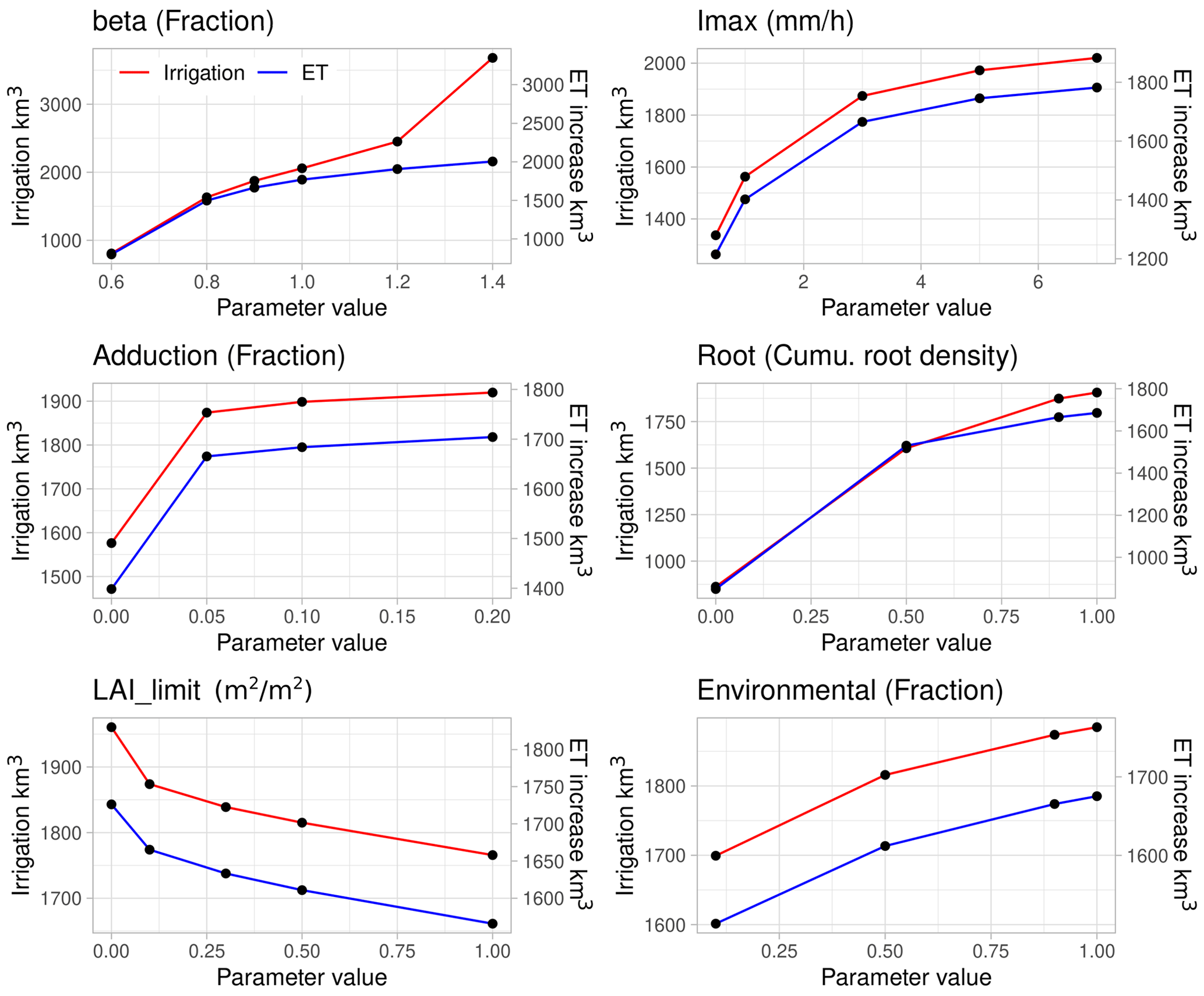
Figure 2Sensitivity of global irrigation volumes and increase in the evapotranspiration (km3) to changes in parameter values for the year 2000, using short simulations. Secondary y axis correspond to ET increase values compared to the simulation with no irrigation. Note that the y axis scales differ between parameters.
Figure 2 shows that β is the parameter with the strongest effect on the global mean irrigation rate, followed by the cumulative root density threshold Rootlim, Imax and the fraction of stream storage available for adduction a1,add. The fraction of water storage left for the ecosystems (called “Environmental” in Fig. 2; aj) has a more limited effect, suggesting that in many irrigated areas, there is enough water from surface and groundwater to fulfill the irrigation requirements. Finally, the LAI limit, LAIlim, to trigger irrigation has a weaker effect than the other parameters. In the case of ET increase (Fig. 2; blue line), the sensitivity to the different parameters is similarly hierarchized, although the magnitude is not necessarily the same. Also note that the effect on irrigation efficiency (i.e., ratio of ET increase to irrigation amount) is different for β values higher than 1.0 and for Rootlim values higher than 0.5. This implies that the fraction of irrigation water that becomes runoff or deep drainage is more important.
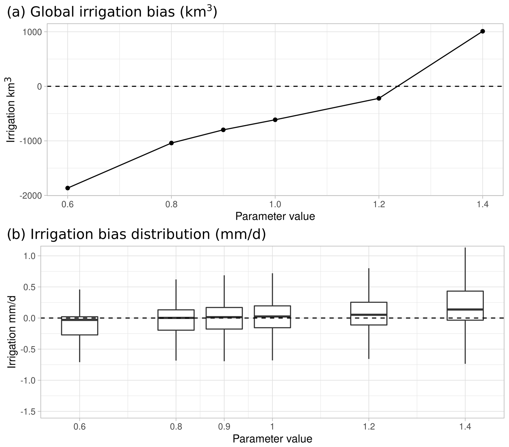
Figure 3Calibration of β value with the Sacks et al. (2009) dataset as the observed value, using outputs from the short simulations. Bias in the total irrigation volume (in km3) by β value (a). Box plot of the bias of irrigation rates in grid cells (in mm d−1) by β value (b).
4.2 Parameter tuning
The sensitivity analysis showed that β has the strongest effect on the simulated irrigation amount and that these effects can induce changes in the irrigation efficiency. Therefore, we explored its behavior in more detail to set a value. Note that we used the chosen reference values for the other parameters. We compared the irrigation rate estimated by ORCHIDEE for the year 2000 in the short tests with the observed irrigation from Sacks et al. (2009) (Fig. 3), using total irrigation volume at global scale and irrigation difference at grid cell scale. When comparing the irrigation water amount at a global scale (in km3 for the year 2000; Fig. 3a), we observe that a value of 1.2 maximizes the irrigation and minimizes the irrigation bias. When we assess the distribution of bias using grid cell values (in mm d−1; Fig. 3b), we observe that for β equal to 0.8, 0.9, or 1, the bias distribution is centered around 0, while it starts to move up for values of 1.2 and 1.4. This behavior can be slightly different, depending on the irrigated fraction (see Fig. S9). For simplicity here, and as a tradeoff between the underestimation of irrigation volume and the spatial distribution of bias, we choose to set β to 0.9 in all irrigated areas. We decided to use the reference values for the other parameters, as they play a minor role according to the sensitivity analysis, and the reference values does not minimize the irrigation amount.
After this analysis, we underline four points. First, this process does not correspond to a proper calibration, as we assumed the uniform parameter values, the number of simulations is low, and the observed data are sparse. The objective of the sensitivity analysis and parameter tuning was to identify key parameters and reduce the underestimation of irrigation by tuning the uniform parameter values. Second, our scheme does not include conveyance losses, although application losses and return flows are represented. As ORCHIDEE determines the water partitioning, some model flaws in hydrologic processes like infiltration or bare soil evaporation could bias the effect in the return flows, in the increase in the ET, and ultimately in the irrigation efficiency. Third, although the one-at-a-time method is suitable, given the computational cost of running an ORCHIDEE simulation, it also has drawbacks and limitations in its analysis (Song et al., 2015); this includes, for instance, its qualitative nature and the lack of the quantification of individual interaction between parameters. Fourth, we use the LUHv2 map, which represents the areas actually irrigated, AAI (a lower value than the areas equipped for irrigation, AEI, which is used in other datasets). We do not consider the effect of prescribed data uncertainty or the effect of meteorological forcing in this analysis.
5.1 Validation of irrigation water withdrawals
Irrigation from the Irr simulation is estimated at 0.049 mm d−1 (2452.5 km3 yr−1) around the year 2000 (Fig. 4a). This estimation is in the lower part of other studies, which range between 2465 and 3755 km3 yr−1 (Pokhrel et al., 2016), and is lower than AQUASTAT estimation of 2735.1 km3 yr−1 around the year 2000 (Frenken and Gillet, 2012). The results suggest that the proposed scheme is adequate to simulate the reported estimations of irrigation, despite the underestimation (−10 % than the 2735.1 km3 yr−1 from AQUASTAT around the year 2000). We note that this estimate is also higher than that of the old irrigation scheme of Guimberteau et al. (2012b), but the scheme proposed here can still benefit from a more robust parameter tuning.
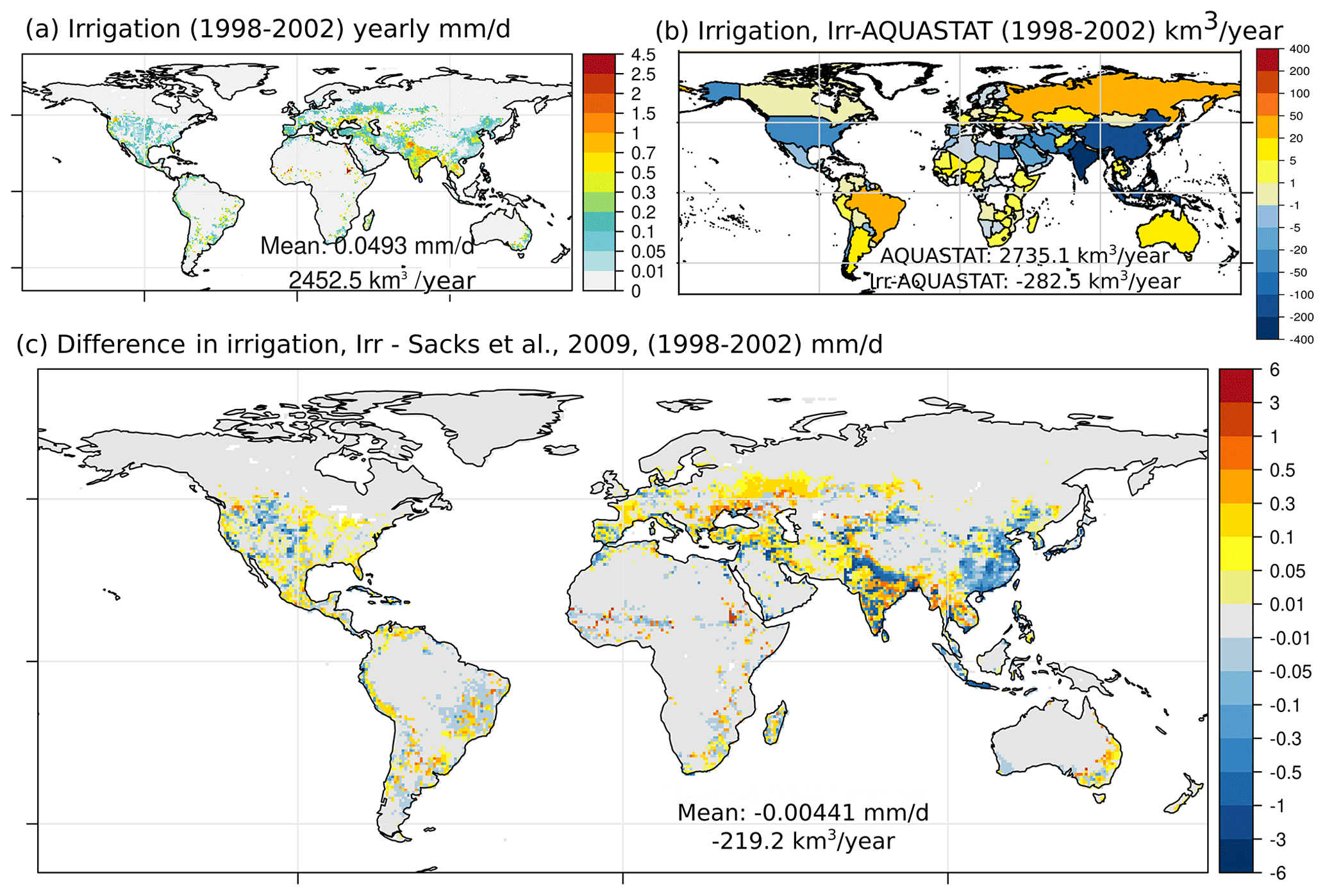
Figure 4Total water withdrawal for irrigation in the Irr simulation with the yearly average for 1998–2002 (a). Difference in water withdrawn for irrigation between Irr (yearly average, 1998–2002) and AQUASTAT value (Frenken and Gillet, 2012) at country level (b). Difference in water withdrawn for irrigation between Irr (yearly average, 1998–2002) and the dataset from Sacks et al. (2009) (c).
At the country scale, Fig. 4b shows that the irrigation module underestimates water withdrawals in the main hotspots of irrigation, i.e., India, China, and the USA, while it overestimates irrigation rates in Africa, Eastern Europe, and Latin America (see also Fig. S1). Such reduced contrasts between highly and weakly irrigated countries could indicate a limitation of the irrigation scheme to represent local irrigation strategies, as our scheme uses global uniform values for all of the parameters. Comparison with the estimation from Sacks et al. (2009) (see Fig. S1) supports this result (−0.004 mm d−1, −219.2 km3 yr−1; Fig. 4c) and allows us to identify the areas where the irrigation bias is the strongest. In India, the Indus Basin presents a strong underestimation, as well as in the northern part of the Ganges–Brahmaputra basin. In China, there is a more widespread underestimation. That is also the case in the western part of the Great Plains in the USA. The other regions present, in general, an overestimation of irrigation withdrawals, which is especially important in some small areas in Africa, in Eastern Europe and north of the Caspian Sea, and in some areas of central Asia. Finally, we note that within a country, it is possible to observe areas with positive and negative bias, for instance in the USA or India. This could also be partially explained by the use of globally uniform values, as there could be important local differences on irrigation strategies within the same country, and it points out the need to assess the irrigation bias at different scales (see Fig. S11).
5.2 Variability in the irrigation rates due to parameter values and input data
The global annual irrigation volumes (Fig. 5a) show a large uncertainty across the simulations due to changes in the parameter values (for instance, −24.7 % between Irr_NoTuned and Irr), but note that the change in irrigation rates at the grid cell scale can have a strong spatial heterogeneity within a country (Fig. 5c), for instance, in India or the USA. The parameter set used in the Irr simulation manages to increase the irrigation rate and to markedly reduce the irrigation bias when compared to the Irr_NoTuned simulation at global scale, even if we may observe both an increase or a decrease on the irrigation rate in the same country locally, for instance, in China (with a marked north–south difference; Fig. 5c; Irr_NoTuned–Irr) or the Indus river basin in Pakistan and India (see Fig. 5c; Irr_NoTuned–Irr). Also, a positive trend in the annual irrigation volume is observed in all simulations. It is caused by the increase in irrigated area and observed in both HID and LUHv2 datasets (see simulations Irr and Irr_LUH). The irrigated area has been identified by Puy et al. (2021) as the main driver of irrigation water withdrawal, and the increase in the prescribed irrigated area in the simulations partly explains the positive trend in the irrigation rate (see Fig. S6).
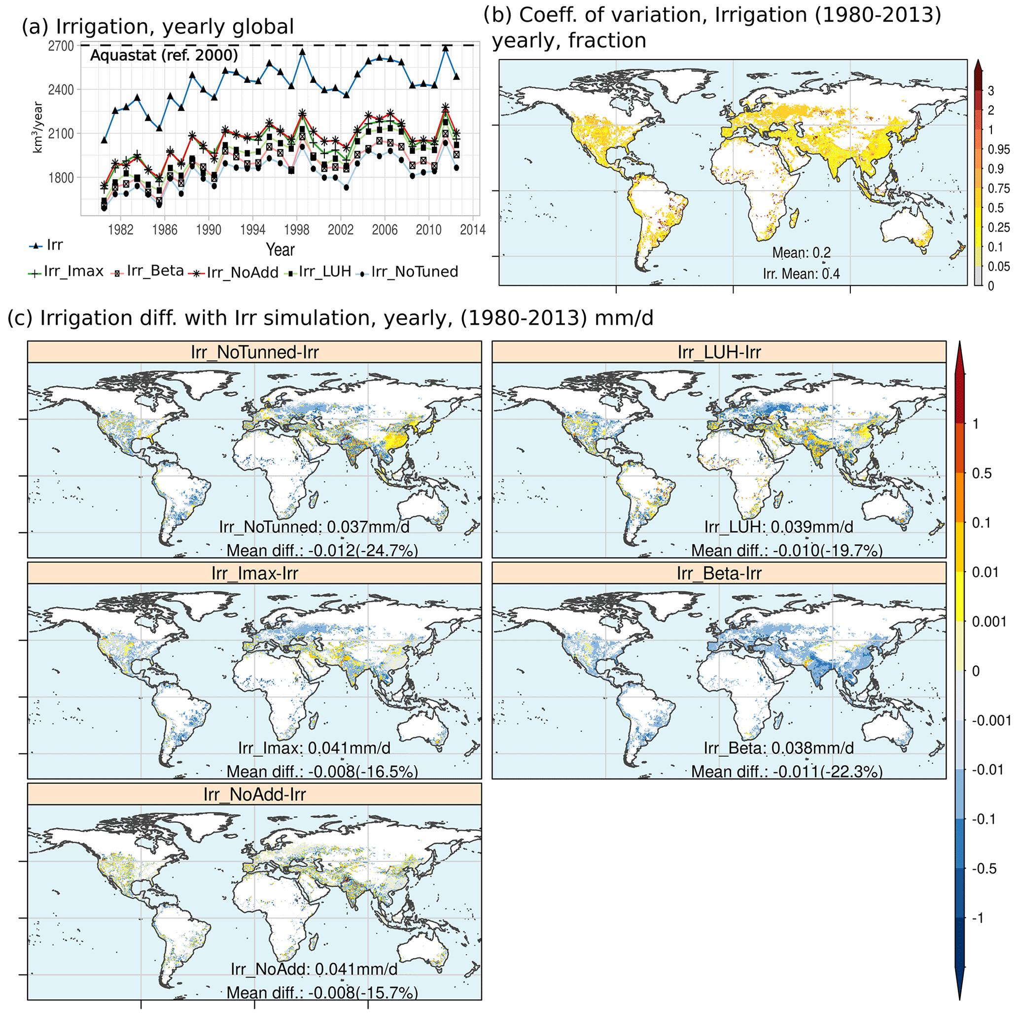
Figure 5Time series of globally averaged irrigation rates simulated by ORCHIDEE (a). Map of the standard deviation of mean irrigation rates from all simulations (in mm d−1) (b). Maps of mean difference between Irr simulation and others for the period 1980–2013 (in mm d−1) (c). Blank areas correspond to grid cells with no irrigated areas.
Based on the mean annual values (Fig. 5c), the β parameter has the largest effect on the mean irrigation rate (−22.3 % when β decreases from 0.9 to 0.75), followed by the change in the input map from HID to LUHv2 (−19.7 %), a lower Imax (−16.5 %), and, finally, no adduction (−15.7 %). From a spatial point of view, the overall reduction in irrigation due to the above changes is not homogeneous, and large areas may even display an increased irrigation rate. The exception is the β parameter, which shows an overall reduction in the irrigation with a lower parameter value, except in the Indus Basin. The Indus River basin is a region that depends on both surface and groundwater for irrigation, and the irrigation demand is one of the most important worldwide (Laghari et al., 2012). In Irr_Beta, a lower β induces a reduction in the water demand in the upper areas of the Indus River basin, increasing the river discharge downstream. More surface water supply in the middle and lower parts of the basin can increase irrigation in these areas, even if the water demand also decreases, because the irrigation deficit; i.e., the difference between demand and supply is still high, despite the demand reduction. We suggest here that the propagation of water supply through the river system can explain part of the heterogeneity in response to other parameter changes.
To estimate the interannual irrigation rate variability, we calculate the coefficient of variation (ratio of standard deviation to the mean; Fig. 5b). We use the pluriannual mean irrigation rate from all simulations with irrigation activated from Table 1. Results highlight a certain homogeneity, but we can identify at least two situations, namely an area of low variability (around 0.25) in Southern Asia, some areas in the Mediterranean and North and South America, and an area of high variability (around 0.75) in northern Europe, North America, Africa, and Australia, with some points where the coefficient of variation is the highest (over 2.0), especially in Africa. The use of global parameter values could explain the relative homogeneity of the coefficient of variation, while regional differences like climate variability and irrigation water demand could explain the existence of these two variability classes.
5.3 Factor analysis: correlation of modeling biases and irrigation classes
Figure 6a shows the bias of ET by class of irrigated fraction at grid cell scale when we compare ORCHIDEE simulations with the FLUXCOM dataset. It shows that the activation of irrigation reduces the ET bias in those areas with high irrigation fractions (also see Fig. S7 for the spatial distribution). For the comparison with GLEAM in Fig. 6b, it shows that the activation of irrigation induces a positive bias in those areas with irrigation. When comparing absolute ET values by irrigation class (Fig. 6c), we observe that NoIrr and GLEAM are similar in all the classes, except for 0 and All (i.e., no irrigated fraction and all grid cells). It means that the differences between NoIrr and GLEAM come from non-irrigated areas. This could suggest a limitation in GLEAM in terms of representing the effects of irrigation on ET rates, as this product does not respond to the presence of irrigated areas. On the other hand, Irr and FLUXCOM box plots are similar for classes 10–20, 20–50, and 50–100. A seasonal assessment on the zonal average values for irrigated areas supports this suggestion (Fig. S7). Thus, from now on, we prioritize FLUXCOM for our analysis regarding the ET bias.
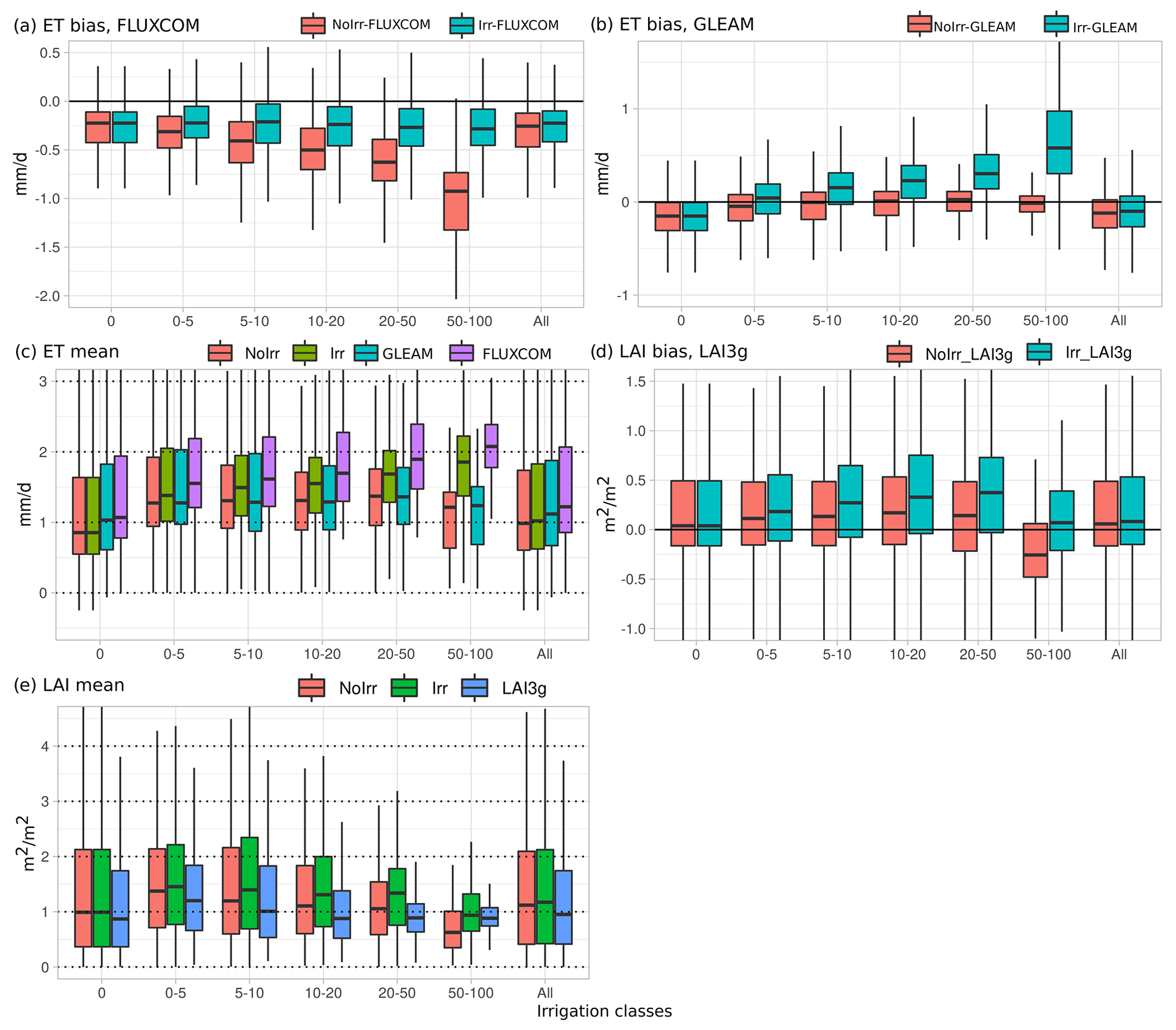
Figure 6Factor analysis of ET bias with FLUXCOM against irrigated fraction classes (a) and with GLEAM (b). Mean ET values of simulations and observed products against irrigated fraction classes (c). LAI bias with LAI3g against irrigated fraction classes (d) and mean LAI values of simulations and observed product against irrigated fraction classes (e).
A similar analysis for the LAI bias and classes of irrigated fraction (Fig. 6d) shows an increase in the LAI difference between ORCHIDEE and LAI3g in the Irr simulation. Also, for all classes, the positive bias in the NoIrr simulation is exacerbated in the Irr simulation, except for the most intensive class (class 50–100), which reduces the negative bias when comparing NoIrr and Irr simulations. It is worth noting that class 50–100, where irrigation is more important, is the only one with a negative bias in NoIrr, and this negative bias is partially reduced when irrigation activities are included (see Fig. S8 for spatial distribution and zonal average values). This is due to less water stress and thus more photosynthesis and biomass production, which is consistent with the decrease in the ET bias for this class. When comparing absolute values between the simulations and the observed product (Fig. 6e), we observe that irrigation activation within ORCHIDEE does not significantly change the distribution of LAI values at a global scale. These results are consistent with the changes that irrigation induce on water fluxes and reservoirs, as well as on water and energy budget (see Figs. S2 and S3).
5.4 Effect of irrigation on TWSAs and river discharge
We now focus on the average TWSA value at the basin scale (Fig. 7). Activation of irrigation induces small changes in TWSAs, which are consistent with changes in TWS between both simulations (Fig. S2). For instance, we observe higher peaks in Huang He when irrigation is activated. Low values also become lower for the Irr simulation in the Huang He basin. In the Ganges Basin, low values are lower as well in the Irr simulation compared to NoIrr. The changes in water pathways and related residence times that explain the changes in TWS between Irr and NoIrr (transfer of water from a reservoir with rapid flows like the streamflow to the soil with a slow flow) could also explain these changes in the TWSA dynamics at a large basin scale. Other basins, like the Nile river basin or the Amu-Darya, show little effect between both simulations, even if extreme peaks values can be overestimated (during 2007 in the Nile) or underestimated (during 2005 and 2006 in Amu-Darya). But note that the model is unable to follow the GRACE trends in basins with negative trends (for instance, Huang He, Indus, or Ganges) or positive trends (Murray River between 2011 and 2014).
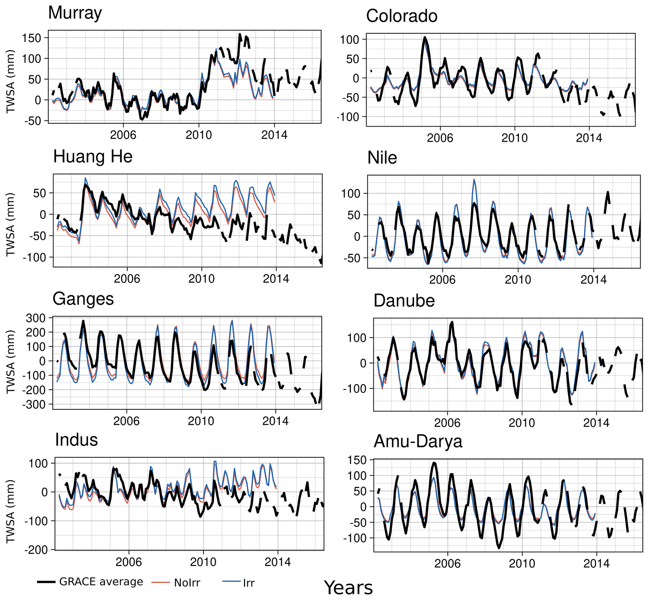
Figure 7Comparison of TWSAs between ORCHIDEE simulations and GRACE datasets in large basins with strong irrigation activities.
The correct simulation of river discharge (Fig. 8) is another challenge in ORCHIDEE and other LSMs (Oki et al., 1999; Ducharne et al., 2003; Guimberteau et al., 2012a; Koirala et al., 2014; Cheruy et al., 2020). Irrigation plays an important role in reducing the average values when we compare NoIrr and Irr simulations (see, for example, the Nile or the Indus rivers, as these results are consistent with those from de Graaf et al., 2014). The main effect of irrigation over the seasonal variations is that peak discharge can occur before in the Irr simulation (for instance, Missouri River or Huang He) or that the decrease after the peak is more rapid, and low values are lower in Irr than in NoIrr (for instance, Colorado River or the Danube). These changes are due to the triggering of irrigation during spring and summer and the corresponding ET increase. It is worth noting that the Irr simulation does not necessarily reduce the discharge bias against GRDC data compared to the NoIrr simulation, with the exception of the Danube (see Table S1 for some goodness-of-fit metrics for the observed and simulated discharge values).
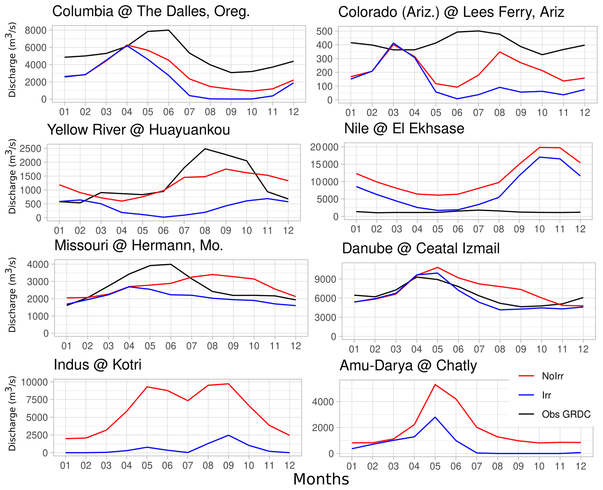
Figure 8Comparison of observed and simulated river discharge in large basins with strong irrigation activities.
5.5 Factor analysis: correlation of irrigation biases and landscape descriptors
We compare biases and errors in irrigation estimates with landscape descriptors that could help explain these modeling errors. We also seek a perspective to increase the realism of the irrigation scheme and reduce the error in irrigation estimation. For the irrigation bias, classes with a high fraction of irrigated paddy rice (for instance, classes 20–50 or 50–100) exhibit a higher bias than classes with small fractions (Fig. 9a). The spatial distribution of irrigated paddy rice is concentrated in Southeast Asia and includes the most irrigated river basins worldwide (see Fig. S5). At the large basin scale (see values in Table S2), the irrigation bias also correlates well with the capacity of dams used for irrigation (Fig. 9b) if we retire a single outlier corresponding to the Nile river basin (r value without the outlier is −0.55).
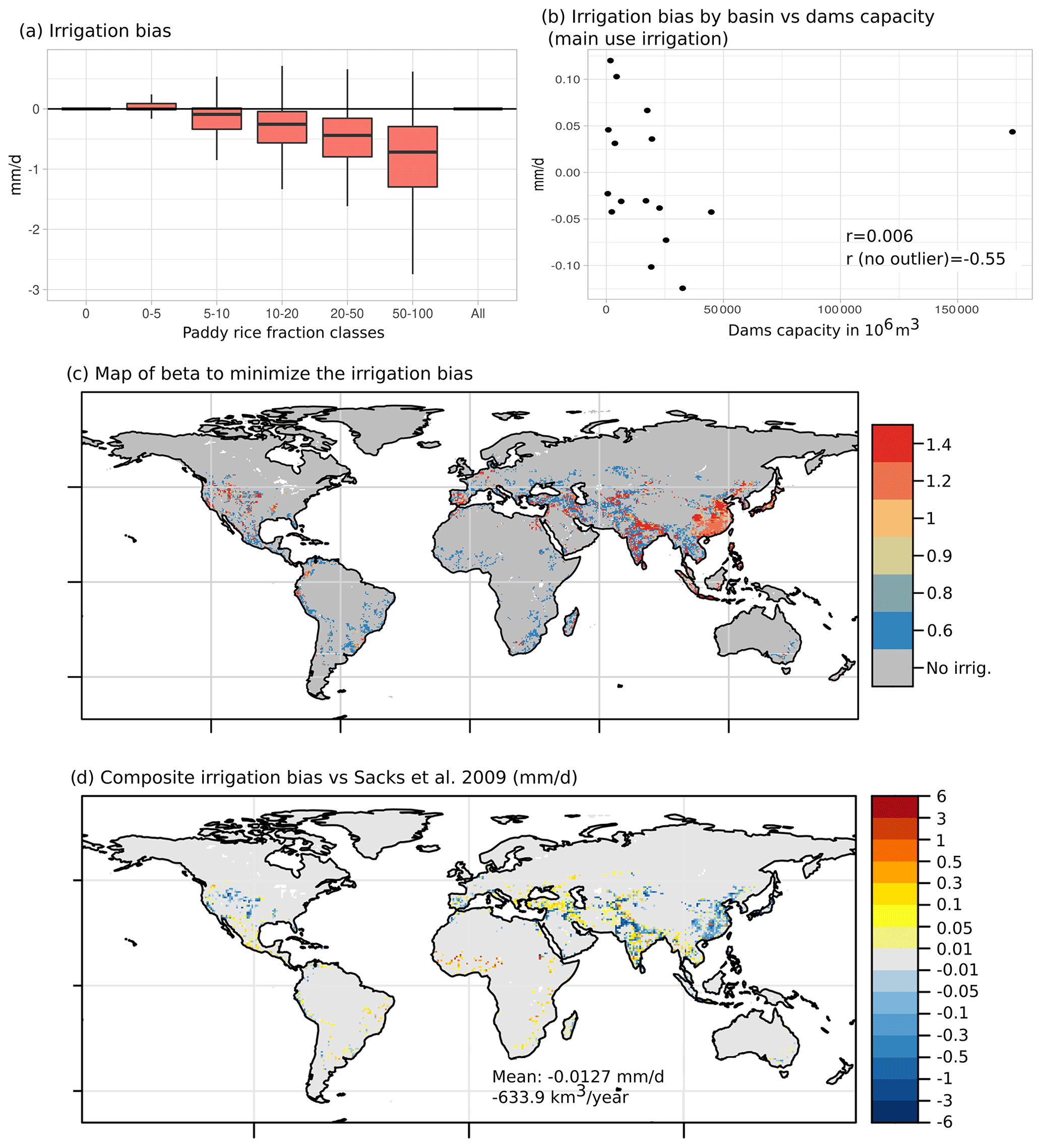
Figure 9Factor analysis of irrigation rate bias with data from Sacks et al. (2009) against irrigated paddy rice classes (a). Basin average value of irrigation bias against dam capacity (b). Map of β that minimizes the irrigation bias, according to the short simulations (c), and corresponding map of minimum irrigation bias, according to the β value in panel (c) (in mm d−1) (d).
The correlation between paddy rice and irrigation bias suggests the need to explicitly represent paddy irrigation at global scale. Thus, we add an assessment of the β value and irrigation bias, using the short simulations used on the parameter tuning (see Sect. 4). We use all simulations with changes in the β parameter from Table 2. Then, we build a composite map of the β value that minimizes the irrigation bias at a grid cell scale (Fig. 9c) and then we show the corresponding irrigation bias as compared to the Sacks et al. (2009) dataset. The results roughly show at least two classes for β, with the first with values of 1.2 and 1.4 (for instance, China and north India) and the second with values of 0.6. Using at least two β values is not enough to reduce the irrigation bias at a global scale, but it has an important effect on the spatial distribution of the irrigation bias in Southern Asia, the region with the largest paddy rice area. These results suggest that the β parameter should have at least two values, namely 1.3 in areas with paddy rice and 0.6 in the rest of the irrigated areas. But note that the data used for this analysis correspond to a single year, i.e., the year 2000. Also, regional characteristics, like more than one harvest of paddy rice due to optimal climate conditions, are not taken into account in this analysis but could also help to explain the irrigation underestimation in our estimations (Yin et al., 2020).
In this study, we implemented a new global irrigation scheme inside the ORCHIDEE land surface model, based on previous work from Yin et al. (2020), in China. While we found a reduction in some modeling biases when irrigation is activated, we also identified at least four types of limitations in our modeling framework that can affect the estimates of irrigation or the effects of irrigation on other variables inside the land surface model.
-
The irrigation scheme exhibits some shortcomings that may bias the estimated irrigation amount, namely the use of a single irrigation technique, simplified rules to trigger irrigation and allocate the available water, the joint representation of rainfed and irrigated crops within the same soil column, and the non-representation of conveyance losses, although losses due to return flows are represented.
-
The parameter tuning is overly simplistic. As a first step, we considered globally uniform parameters, which is overly simplistic, although spatially distributed values would allow us to better describe the local features of irrigation systems, as shown by the spatial variations in an optimized β map, and the dependence of the local irrigation bias on the fraction of paddy rice.
-
We also use a single meteorological forcing dataset and a single year to characterize the observed irrigation values. This contributes to biasing the parameter adjustment process by taking uncertain data (meteorological forcing and reference irrigation) as certain.
-
The ORCHIDEE model exhibits many uncertainties that are not related to the irrigation scheme but ultimately impact the irrigation withdrawals and efficiency (defined here as the ratio of additional ET due to irrigation to water withdrawal) and the temporal dynamics of irrigation. One particular uncertainty comes from the overestimation of bare soil evaporation (Cheruy et al., 2020) that we are presently trying to correct in ORCHIDEE. Other uncertainties result from the inherent simplifications of any model. In ORCHIDEE, they include the use of a single soil texture in each grid cell of only two kinds of crops, with simplified phenology and crop calendars, and the choices made to simulate infiltration and evaporative processes.
These shortcomings and limitations could induce positive or negative biases in the simulated regional irrigation amounts; this as a result of differences in regional landscape, hydroclimatic conditions, and local irrigation practices not well represented or absent in our scheme. For example, the missing representation of paddy irrigation induces under-irrigation in paddy rice areas, the joint representation of rainfed and irrigated crops induces over-irrigation in areas with other crop types and irrigation techniques, and the simplistic parameter tuning could tend to minimize the overall net bias while increasing the regional biases. These limitations (some shared with other global LSMs) call for further model developments that aim at a better representation of the water supply (fossil groundwater and water adduction, to list two examples mentioned in the results) and the water demand (a separate water budget for irrigated areas, the inclusion of other irrigation techniques, and new irrigation rules, such as irrigation before sowing or interruption of irrigation before harvest). In addition to the improvements noted here that focus on model developments, the irrigation representation can be improved using new input datasets and regional parameter values to include local practices (if these datasets exist at the coarse model resolution in the global domain and for historical period or future scenarios), for instance, to prescribe regional β values or to prescribe the start and end of the growing season.
The model estimates the irrigation water demand by calculating a soil moisture deficit according to a user-defined soil moisture target. Besides, it constrains the actual irrigation rate using the available water supply. The water supply takes into account the facility to access surface or underground water sources according to local infrastructure and environmental restrictions. Note that this environmental restriction is a simplification compared to the complex methods used in the real world to estimate environmental flow requirements, and other more robust approaches exist (for instance, in Hanasaki et al., 2008a, providing monthly environmental flow requirements). Strict environmental requirements could reduce the surface water supply and thus the irrigation rate (Hanasaki et al., 2008b).
For the facility to access the water sources, we use two static factors based on local infrastructure, while water allocation is dynamic and can change according to water availability (de Graaf et al., 2014) as well as economic and societal aspects (D'Odorico et al., 2020). The irrigation scheme also allows the adduction of water from neighboring grid cells, which can be important in areas of China and India (Laghari et al., 2012; Yin et al., 2021), where surface water is intensively used. This representation of water adduction, however, is very simple, and could be improved by including human water management and dams operation, as in Zhou et al. (2021), where the supply and demand network is operated as a system, taking into account some constraints like topography and environmental flow (Hanasaki et al., 2018).
Regarding the water demand, we observed that the conditions to trigger and stop irrigation, although controlled by four parameters, may seem too simple in our scheme, especially when compared to specialized irrigation models like the new irrigation scheme in LSM CLM5 (Yao et al., 2022), which includes multiple irrigation techniques, or the ISBA LSM (Druel et al., 2022), which implements complex sets of rules to represent different irrigation strategies. Some rules could change the moment when irrigation is triggered and increase the amount (for instance, allowing irrigation some days before the crop emergence) or decrease it (for instance, preventing irrigation during the maturity of the crop, shortening the growing season, or preventing continuous irrigation during more than a certain number of days). Implementing these sets of rules for irrigation strategies in ORCHIDEE is feasible; for instance, the definition of the growing season (with the trigger of irrigation before sowing and stopping before harvesting) could be based on the prescription of the start and end dates, as done by Yin et al. (2020), or could use the phenology information simulated by the model (as in the version used here or using a crop-specific module as in Wu et al., 2016). But defining the set of rules and parameter values would need a careful tuning and evaluation process with local data at a sub-yearly scale.
Despite these limitations, the evaluated irrigation scheme produces acceptable estimations of yearly irrigation withdrawals on a global mean basis, but it underestimates irrigation volumes in areas of China, India, and the USA (the most irrigated areas). Our estimations are affected by the uncertainty about global parameter values that are assumed to be uniform and on the map of irrigated fractions (Puy et al., 2021). We show that the lack of paddy rice irrigation could contribute to the underestimation of irrigation in southern Asia, as the paddy technique needs the inundation of the field and maintains a saturated soil during at least 80 % of the crop growth (de Vrese and Hagemann, 2018). The irrigation module of MATSIRO LSM, called MAT-HI and HiWG-MAT (Pokhrel et al., 2012, 2015), already implemented an explicit representation of paddy rice irrigation by setting a higher soil moisture target for rice than for other crops. An explicit paddy representation was also implemented in ORCHIDEE-CROP (Yin et al., 2020) at a regional scale by implementing a pond for paddy rice and using a water level target, but it uses detailed crop information that is not easy to access at a global scale. A surrogate approach in our simpler irrigation scheme could be to use at least two β values, one for paddy rice and another one for other crops, as suggested by the composite map of β values to minimize the irrigation bias.
An outcome of our study is to reveal that the GLEAM values do not exhibit a significant sensitivity of ET to the presence of irrigated areas. This suggests that GLEAM is not suitable for estimating ET rates in irrigated areas. For instance, coupled simulations using CLM4 in northern India showed a strong modeling underestimation of ET rates, even with no irrigation (Fowler et al., 2018). When we compare the simulations with the FLUXCOM product, the activation of irrigation leads to a reduction in the negative evapotranspiration bias, but the use of a single soil column in ORCHIDEE for both rainfed and irrigated crops could induce an overestimation of the ET increase (see Fig. S11; in some cases, the irrigation efficiency by country is too high). The ET bias improvement is particularly substantial in heavily irrigated areas, where the simulated LAI is also improved by irrigation (which reduces the negative LAI bias there). These results show the benefits of including an irrigation scheme to partially reduce some modeling biases, especially in intensively irrigated areas, and are consistent with the multivariate evaluation of ORCHIDEE done in Mizuochi et al. (2021).
ET and LAI are two important drivers of land–atmosphere coupling via water, energy, and momentum transfer (Seneviratne et al., 2010; Greve et al., 2019), but there is evidence that the effects on ET and LAI due to human land cover change and landscape management are not monotonic (Sterling et al., 2013). The sensitivity of these drivers to irrigation calls for further studies in coupled mode to explore the joint evolution of climate, land surface fluxes, and the use of water resources. Some studies focuses on the effects of irrigation on climate and land surface fluxes for the historical climate (Boucher et al., 2004; Sacks et al., 2009; Puma and Cook, 2010; Guimberteau et al., 2012b; Cook et al., 2015; Thiery et al., 2017; Al‐Yaari et al., 2022), but to the best of our knowledge, that is not the case for the future climate under different scenarios.
In contrast to the effects on ET and LAI, the effect of irrigation on land surface hydrology is rather weak. For discharge, the activation of irrigation logically reduces river discharge because of the surface and groundwater withdrawal for irrigation. This reduction does not necessarily improve the model performance to fit observed values, with the exception of the Danube river basin. Multiple causes could explain the incorrect simulation of discharge dynamics in ORCHIDEE, even when irrigation is activated. For instance, uncertainties resulting from the atmospheric forcing are not assessed here, while they are known to affect the yearly and seasonal values of discharge (Guimberteau et al., 2012a; Decharme et al., 2019). Also, a wrong ET estimation, errors in snow dynamics, and the lack of permafrost representation contribute to the mismatches (Cheruy et al., 2020). Finally, a lack of representation of other anthropogenic processes, like dam management (Fig. 9) and water withdrawal for other economic sectors and other uses, could explain the differences in the seasonal discharge dynamics between ORCHIDEE and observed data in some basins (Pokhrel et al., 2016).
The effect of irrigation on simulated TWSAs is weak. In some large river basins, we observed increases in low values in areas with significant surface water supply. But even when irrigation is activated, ORCHIDEE is not able to follow the trends exhibited by GRACE datasets, for instance in Huang He and Indus River basin, two heavily irrigated areas where water depletion has been related to groundwater pumping for irrigation (Rodell et al., 2018; Yin et al., 2020). There are probably multiple causes for the inability of LSMs to capture large negative decadal water storage trends (Scanlon et al., 2018), starting with the underestimation of irrigation rates at country level and grid cell scale (Fig. 4). Glacier loss misrepresentation in ORCHIDEE could also explain part of the differences to observed negative trends in some basins, for instance in the Indus and Ganges basins that depend on water flow from the Himalaya mountains (Rodell et al., 2018). And of course, errors in the partitioning between the different water fluxes in ORCHIDEE (Cheruy et al., 2020; Mizuochi et al., 2021) contribute to the problems in both simulations (NoIrr and Irr).
We also underline the lack of fossil groundwater abstraction in ORCHIDEE as a very likely cause for the underestimation of irrigation rates and TWSA trend mismatch. Fossil groundwater, also called nonrenewable groundwater, is important in semiarid areas like Pakistan and the Middle East and contributes nearly 20 % to the gross irrigation water demand for the year 2000 (Wada et al., 2012). As the irrigation scheme represents abstractions from shallow aquifers but not from fossil sources, it probably restrains irrigation too often due to a supply shortage and thus could have problems fitting the negative trend in those areas with heavy groundwater use, as already reported by Yin et al. (2020) for China. But we must add that the estimation of fossil groundwater use is challenging. For instance, an assessment of the TWSA trends of residuals between our simulation and GRACE shows differences with the estimates of groundwater depletion from Wada et al. (2012) in some countries (see Table S3). Underestimation of irrigation rates and uncertainties arising from flux partitioning and from meteorological data would also affect the estimations of fossil groundwater abstraction. So far, we cannot explain to which extent each one of these possible causes participates in the misrepresentation of GRACE TWSA trends by ORCHIDEE.
Our results show that the new irrigation scheme helps simulate acceptable land surface conditions and fluxes in irrigated areas for ET and LAI, but they also show that inclusion of irrigation alone is not necessarily sufficient for a good fit between the simulated values of TWSAs and discharge and observed products. Including additional anthropogenic processes could help to reduce some of these biases. For instance, dam management and fossil irrigation withdrawal could increase the water supply in some basins during dry months or years, thus increasing the irrigation amount in areas with high irrigation demand and water supply shortage. At the same time, these processes may have an impact on river discharge dynamics and could help to represent the misrepresentation of TWSA trends in some areas.
We implemented a global irrigation scheme within ORCHIDEE LSM with a simple representation of the environmental restriction, water allocation rules based on local infrastructure, and water adduction from nonlocal water reservoirs. We compared the irrigation estimates to reported values of irrigation withdrawal, and then we compared the outputs with and without irrigation to observed products of ET, LAI, TWSAs and discharge. Our results highlight how the inclusion of irrigation can reduce some modeling biases, especially for ET and LAI, but they also underline the difficulties in representing irrigation on a large scale using a simple scheme and limited information.
The model could still benefit from improvements in parameter tuning by explicitly representing paddy rice irrigation. Paddy irrigation could decrease the irrigation bias in areas of southern Asia by increasing the irrigation demand. Dam management representation and the inclusion of nonrenewable groundwater use could also reduce negative biases in some heavily regulated basins by increasing the water supply. These three aspects could change the spatial distribution of the ET and LAI increases within the model. For TWSAs and discharge, the inclusion of processes like dam management or fossil groundwater use could help to represent observed seasonal dynamics and trends that the model is not currently able to represent.
Finally, we remember that LSMs are commonly used in a coupled mode with climate models, and irrigation can have an impact on some atmospheric variables via changes in the latent heat flux and leaf area index. Thus, the results obtained here encourage the use of coupled simulations to explore the joint evolution of climate under the ongoing climate change (for historical and especially for future periods), water resources, and irrigation activities. While there is an increasing body of literature that explores the coupling of irrigation and climate for the historical period, to the best of our knowledge, that is not the case for future scenarios. Coupled climate simulations for future scenarios could help to foresee potential changes in the joint long-term evolution of water resources use and climate and might help to identify possible social consequences.
The version of the ORCHIDEE LSM used for this study corresponds to tag 2.2, revision 7709 and is freely available from https://forge.ipsl.jussieu.fr/orchidee/log/branches/ORCHIDEE_2_2/ (last access: 16 June 2023, Arboleda et al., 2023). It is provided under a CeCILL-C license (French equivalent to the LGPL license).
The data from the ORCHIDEE simulations used for this study are freely accessible at https://doi.org/10.5281/zenodo.8014430 (Arboleda-Obando et al., 2023). FLUXCOM is available at https://www.bgc-jena.mpg.de/geodb/projects/Home.php (Jung et al., 2019) after registration. GLEAM is available at https://www.gleam.eu/ (Martens et al., 2017) after registration. LAI3g is available at https://doi.org/10.3334/ORNLDAAC/1653 (Mao and Yan, 2019). Monthly discharge data from the GRDC are available at https://www.bafg.de/GRDC/EN/Home/homepage_node.html (GRDC, 2024). For TWSAs, the CSR dataset is available at https://www2.csr.utexas.edu/grace/RL06_mascons.html (Save et al., 2016), Tellus is available at https://doi.org/10.5067/TEMSC-3JC63 (Wiese et al., 2023), and GSFC is available at https://earth.gsfc.nasa.gov/geo/data/grace-mascons (Loomis et al., 2019). HID dataset is available at https://mygeohub.org/publications/8/2 (Siebert et al., 2015), and LUHv2 is available at https://luh.umd.edu/ (Hurtt et al., 2020). MIRCA2000 is available at https://doi.org/10.5281/zenodo.7422506 (Portmann et al., 2010b). GRanD dataset is available at https://sedac.ciesin.columbia.edu/data/set/grand-v1-dams-rev01 (Lehner et al., 2011). For analysis, we used standard packages from R v.4.0.4 (R Core Team, 2016), https://www.R-project.org/ (last access: 3 December 2022).
The supplement related to this article is available online at: https://doi.org/10.5194/gmd-17-2141-2024-supplement.
All the authors participated in the initial development of the irrigation scheme. PFAO and AD implemented the scheme in ORCHIDEE's code, ran the simulations, and evaluated the model. PFAO wrote the first draft. All the authors contributed to interpreting the results, discussing the findings, and improving the final version of the paper.
The contact author has declared that none of the authors has any competing interests.
Publisher's note: Copernicus Publications remains neutral with regard to jurisdictional claims made in the text, published maps, institutional affiliations, or any other geographical representation in this paper. While Copernicus Publications makes every effort to include appropriate place names, the final responsibility lies with the authors.
We would like to thank the editor and two anonymous reviewers for their helpful comments and observations, which contributed to improve the paper. This research was part of the doctoral project of Pedro F. Arboleda-Obando, funded by EUR IPSL-CGS (ANR Investissements d'Avenir; grant no. ANR-11-IDEX-0004-17-EURE-0006). This work has also received support from project BLUEGEM (grant no. ANR-21-SOIL-0001). The simulations were done using the IDRIS computational facilities (Institut du Développement et des Ressources en Informatique Scientifique, CNRS, France), under the allocation 2022-[AD010113599R1]. We thank William Sacks for sharing the gridded maps on irrigation withdrawal for the year 2000.
This research has been supported by the Agence Nationale de la Recherche (grant nos. ANR-11-IDEX-0004-17-EURE-0006 and ANR-21-SOIL-0001).
This paper was edited by Sam Rabin and reviewed by two anonymous referees.
Allen, G. R., Pereira, L. S., Raes, D., and Smith, M.: Evapotranspiración del cultivo: Guias para la determinación de los requerimientos de agua de los cultivos., FAO: Estudios FAO Riego y Drenaje, 56, 297, https://doi.org/10.1590/1983-40632015v4529143, 2006. a
Al-Yaari, A., Ducharne, A., Cheruy, F., Crow, W. T., and Wigneron, J. P.: Satellite-based soil moisture provides missing link between summertime precipitation and surface temperature biases in CMIP5 simulations over conterminous United States, Sci. Rep., 9, 1–12, https://doi.org/10.1038/s41598-018-38309-5, 2019. a
Al‐Yaari, A., Ducharne, A., Thiery, W., Cheruy, F., and Lawrence, D.: The Role of Irrigation Expansion on Historical Climate Change: Insights From CMIP6, Earth's Future, 10, 1–29, https://doi.org/10.1029/2022EF002859, 2022. a, b
Arboleda, P., Ducharne, A., Yin, Z., and Ciais, P.: ORCHIDEE_2_2 revision 7709/, Zenodo [code], https://doi.org/10.5281/zenodo.8136558, 2023. a
Arboleda-Obando, P. F., Ducharne, A., Yin, Z., and Ciais, P.: Validation of a new global irrigation scheme in the ORCHIDEE land surface model – Dataset, Zenodo [data set], https://doi.org/10.5281/zenodo.8014430, 2023. a
Barella-Ortiz, A., Polcher, J., Tuzet, A., and Laval, K.: Potential evaporation estimation through an unstressed surface-energy balance and its sensitivity to climate change, Hydrol. Earth Syst. Sci., 17, 4625–4639, https://doi.org/10.5194/hess-17-4625-2013, 2013. a
Boucher, O., Myhre, G., and Myhre, A.: Direct human influence of irrigation on atmospheric water vapour and climate, Clim. Dynam., 22, 597–603, https://doi.org/10.1007/s00382-004-0402-4, 2004. a
Boucher, O., Servonnat, J., Albright, A. L., Aumont, O., Balkanski, Y., Bastrikov, V., Bekki, S., Bonnet, R., Bony, S., Bopp, L., Braconnot, P., Brockmann, P., Cadule, P., Caubel, A., Cheruy, F., Codron, F., Cozic, A., Cugnet, D., D'Andrea, F., Davini, P., Lavergne, C., Denvil, S., Deshayes, J., Devilliers, M., Ducharne, A., Dufresne, J., Dupont, E., Éthé, C., Fairhead, L., Falletti, L., Flavoni, S., Foujols, M., Gardoll, S., Gastineau, G., Ghattas, J., Grandpeix, J., Guenet, B., Guez, Lionel, E., Guilyardi, E., Guimberteau, M., Hauglustaine, D., Hourdin, F., Idelkadi, A., Joussaume, S., Kageyama, M., Khodri, M., Krinner, G., Lebas, N., Levavasseur, G., Lévy, C., Li, L., Lott, F., Lurton, T., Luyssaert, S., Madec, G., Madeleine, J., Maignan, F., Marchand, M., Marti, O., Mellul, L., Meurdesoif, Y., Mignot, J., Musat, I., Ottlé, C., Peylin, P., Planton, Y., Polcher, J., Rio, C., Rochetin, N., Rousset, C., Sepulchre, P., Sima, A., Swingedouw, D., Thiéblemont, R., Traore, A. K., Vancoppenolle, M., Vial, J., Vialard, J., Viovy, N., and Vuichard, N.: Presentation and Evaluation of the IPSL‐CM6A‐LR Climate Model, J. Adv. Model. Earth Sy., 12, 1–52, https://doi.org/10.1029/2019MS002010, 2020. a, b, c, d
Campoy, A., Ducharne, A., Cheruy, F., Hourdin, F., Polcher, J., and Dupont, J. C.: Response of land surface fluxes and precipitation to different soil bottom hydrological conditions in a general circulation model, J. Geophys. Res.-Atmos., 118, 10725–10739, https://doi.org/10.1002/jgrd.50627, 2013. a
Cheruy, F., Ducharne, A., Hourdin, F., Musat, I., Vignon, E., Gastineau, G., Bastrikov, V., Vuichard, N., Diallo, B., Dufresne, J., Ghattas, J., Grandpeix, J., Idelkadi, A., Mellul, L., Maignan, F., Menegoz, M., Ottlé, C., Peylin, P., Servonnat, J., Wang, F., and Zhao, Y.: Improved near surface continental climate in IPSL‐CM6A‐LR by combined evolutions of atmospheric and land surface physics, J. Adv. Model. Earth Sy., 12, e2019MS002005, https://doi.org/10.1029/2019MS002005, 2020. a, b, c, d, e
Chiarelli, D. D., Passera, C., Rosa, L., Davis, K. F., D'Odorico, P., and Rulli, M. C.: The green and blue crop water requirement WATNEEDS model and its global gridded outputs, Sci. Data, 7, 1–9, https://doi.org/10.1038/s41597-020-00612-0, 2020. a
Cook, B. I., Shukla, S. P., Puma, M. J., and Nazarenko, L. S.: Irrigation as an historical climate forcing, Clim. Dynam., 44, 1715–1730, https://doi.org/10.1007/s00382-014-2204-7, 2015. a, b, c
Decharme, B., Delire, C., Minvielle, M., Colin, J., Vergnes, J., Alias, A., Saint‐Martin, D., Séférian, R., Sénési, S., and Voldoire, A.: Recent Changes in the ISBA‐CTRIP Land Surface System for Use in the CNRM‐CM6 Climate Model and in Global Off‐Line Hydrological Applications, J. Adv. Model. Earth Sy., 11, 1207–1252, https://doi.org/10.1029/2018MS001545, 2019. a
de Graaf, I., van Beek, L., Wada, Y., and Bierkens, M.: Dynamic attribution of global water demand to surface water and groundwater resources: Effects of abstractions and return flows on river discharges, Adv. Water Resour., 64, 21–33, https://doi.org/10.1016/j.advwatres.2013.12.002, 2014. a, b
de Oliveira, L. V.: Irrigation in the ORCHIDEE model : Evaluating inputs and results in metropolitan France, Internship report, Ecole Normale Superieure, 2022. a
de Rosnay, P., Polcher, J., Bruen, M., and Laval, K.: Impact of a physically based soil water flow and soil-plant interaction representation for modeling large-scale land surface processes, J. Geophys. Res.-Atmos., 107, ACL 3–1–ACL 3–19, https://doi.org/10.1029/2001JD000634, 2002. a, b
de Rosnay, P., Polcher, J., Laval, K., and Sabre, M.: Integrated parameterization of irrigation in the land surface model ORCHIDEE. Validation over Indian Peninsula, Geophys. Res. Lett., 30, 1986, https://doi.org/10.1029/2003GL018024, 2003. a
de Vrese, P. and Hagemann, S.: Uncertainties in modelling the climate impact of irrigation, Clim. Dynam., 51, 2023–2038, https://doi.org/10.1007/s00382-017-3996-z, 2018. a
Döll, P., Hoffmann-Dobrev, H., Portmann, F. T., Siebert, S., Eicker, A., Rodell, M., Strassberg, G., and Scanlon, B. R.: Impact of water withdrawals from groundwater and surface water on continental water storage variations, J. Geodynam., 59-60, 143–156, https://doi.org/10.1016/j.jog.2011.05.001, 2012. a, b, c
D'Odorico, P., Chiarelli, D. D., Rosa, L., Bini, A., Zilberman, D., and Rulli, M. C.: The global value of water in agriculture, P. Natl. Acad. Sci. USA, 117, 21985–21993, https://doi.org/10.1073/pnas.2005835117, 2020. a
d'Orgeval, T., Polcher, J., and de Rosnay, P.: Sensitivity of the West African hydrological cycle in ORCHIDEE to infiltration processes, Hydrol. Earth Syst. Sci., 12, 1387–1401, https://doi.org/10.5194/hess-12-1387-2008, 2008. a, b
Druel, A., Munier, S., Mucia, A., Albergel, C., and Calvet, J.-C.: Implementation of a new crop phenology and irrigation scheme in the ISBA land surface model using SURFEX_v8.1, Geosci. Model Dev., 15, 8453–8471, https://doi.org/10.5194/gmd-15-8453-2022, 2022. a
Ducharne, A., Golaz, C., Leblois, E., Laval, K., Polcher, J., Ledoux, E., and De Marsily, G.: Development of a high resolution runoff routing model, calibration and application to assess runoff from the LMD GCM, J. Hydrol., 280, 207–228, https://doi.org/10.1016/S0022-1694(03)00230-0, 2003. a
Felfelani, F., Lawrence, D. M., and Pokhrel, Y.: Representing Intercell Lateral Groundwater Flow and Aquifer Pumping in the Community Land Model, Water Resour. Res., 57, 1–24, https://doi.org/10.1029/2020WR027531, 2021. a, b
Fowler, M. D., Pritchard, M. S., and Kooperman, G. J.: Assessing the impact of Indian irrigation on precipitation in the irrigation-enabled community earth system model, J. Hydrometeorol., 19, 427–443, https://doi.org/10.1175/JHM-D-17-0038.1, 2018. a
Frenken, K. and Gillet, V.: Irrigation water requirement and water withdrawal by country, Tech. rep., Food and Agriculture Organization, Rome, http://www.fao.org/aquastat/en/data-analysis/irrig-water-use/ (last access: 28 February 2024), 2012. a, b, c, d
Grafton, R. Q., Williams, J., and Jiang, Q.: Possible pathways and tensions in the food and water nexus, Earth's Future, 5, 449–462, https://doi.org/10.1002/2016EF000506, 2017. a
GRDC: Homepage, Global Runoff Data Centre [data set], https://grdc.bafg.de/GRDC/EN/Home/homepage_node.html, last access: 6 March 2024. a
Greve, P., Roderick, M. L., Ukkola, A. M., and Wada, Y.: The aridity Index under global warming, Environ. Res. Lett., 14, 124006, https://doi.org/10.1088/1748-9326/ab5046, 2019. a
Guimberteau, M., Drapeau, G., Ronchail, J., Sultan, B., Polcher, J., Martinez, J.-M., Prigent, C., Guyot, J.-L., Cochonneau, G., Espinoza, J. C., Filizola, N., Fraizy, P., Lavado, W., De Oliveira, E., Pombosa, R., Noriega, L., and Vauchel, P.: Discharge simulation in the sub-basins of the Amazon using ORCHIDEE forced by new datasets, Hydrol. Earth Syst. Sci., 16, 911–935, https://doi.org/10.5194/hess-16-911-2012, 2012a. a, b, c
Guimberteau, M., Laval, K., Perrier, A., and Polcher, J.: Global effect of irrigation and its impact on the onset of the Indian summer monsoon, Clim. Dynam., 39, 1329–1348, https://doi.org/10.1007/s00382-011-1252-5, 2012b. a, b, c, d, e, f, g
Haddeland, I., Lettenmaier, D. P., and Skaugen, T.: Effects of irrigation on the water and energy balances of the Colorado and Mekong river basins, J. Hydrol., 324, 210–223, https://doi.org/10.1016/j.jhydrol.2005.09.028, 2006. a
Hanasaki, N., Kanae, S., Oki, T., Masuda, K., Motoya, K., Shirakawa, N., Shen, Y., and Tanaka, K.: An integrated model for the assessment of global water resources – Part 1: Model description and input meteorological forcing, Hydrol. Earth Syst. Sci., 12, 1007–1025, https://doi.org/10.5194/hess-12-1007-2008, 2008a. a, b, c, d
Hanasaki, N., Kanae, S., Oki, T., Masuda, K., Motoya, K., Shirakawa, N., Shen, Y., and Tanaka, K.: An integrated model for the assessment of global water resources – Part 2: Applications and assessments, Hydrol. Earth Syst. Sci., 12, 1027–1037, https://doi.org/10.5194/hess-12-1027-2008, 2008b. a
Hanasaki, N., Yoshikawa, S., Pokhrel, Y., and Kanae, S.: A global hydrological simulation to specify the sources of water used by humans, Hydrol. Earth Syst. Sci., 22, 789–817, https://doi.org/10.5194/hess-22-789-2018, 2018. a
Hoogeveen, J., Faurès, J.-M., Peiser, L., Burke, J., and van de Giesen, N.: GlobWat – a global water balance model to assess water use in irrigated agriculture, Hydrol. Earth Syst. Sci., 19, 3829–3844, https://doi.org/10.5194/hess-19-3829-2015, 2015. a, b
Hurtt, G. C., Chini, L., Sahajpal, R., Frolking, S., Bodirsky, B. L., Calvin, K., Doelman, J. C., Fisk, J., Fujimori, S., Klein Goldewijk, K., Hasegawa, T., Havlik, P., Heinimann, A., Humpenöder, F., Jungclaus, J., Kaplan, J. O., Kennedy, J., Krisztin, T., Lawrence, D., Lawrence, P., Ma, L., Mertz, O., Pongratz, J., Popp, A., Poulter, B., Riahi, K., Shevliakova, E., Stehfest, E., Thornton, P., Tubiello, F. N., van Vuuren, D. P., and Zhang, X.: Harmonization of global land use change and management for the period 850–2100 (LUH2) for CMIP6, Geosci. Model Dev., 13, 5425–5464, https://doi.org/10.5194/gmd-13-5425-2020, 2020 (data available at: https://luh.umd.edu/, last access: 6 March 2024). a, b, c
Jägermeyr, J., Gerten, D., Heinke, J., Schaphoff, S., Kummu, M., and Lucht, W.: Water savings potentials of irrigation systems: global simulation of processes and linkages, Hydrol. Earth Syst. Sci., 19, 3073–3091, https://doi.org/10.5194/hess-19-3073-2015, 2015. a, b, c
Jung, M., Koirala, S., Weber, U., Ichii, K., Gans, F., Camps-Valls, G., Papale, D., Schwalm, C., Tramontana, G., and Reichstein, M.: The FLUXCOM ensemble of global land-atmosphere energy fluxes, Sci. Data, 6, 74, https://doi.org/10.1038/s41597-019-0076-8, 2019 (data available at: https://www.bgc-jena.mpg.de/geodb/projects/Home.php, last access: 28 February 2024). a, b, c
Klein Goldewijk, K., Beusen, A., Doelman, J., and Stehfest, E.: Anthropogenic land use estimates for the Holocene – HYDE 3.2, Earth Syst. Sci. Data, 9, 927–953, https://doi.org/10.5194/essd-9-927-2017, 2017. a, b
Koirala, S., Yeh, P. J., Hirabayashi, Y., Kanae, S., and Oki, T.: Global‐scale land surface hydrologic modeling with the representation of water table dynamics, J. Geophys. Res.-Atmos., 119, 75–89, https://doi.org/10.1002/2013JD020398, 2014. a
Krinner, G., Viovy, N., de Noblet-Ducoudré, N., Ogée, J., Polcher, J., Friedlingstein, P., Ciais, P., Sitch, S., and Prentice, I. C.: A dynamic global vegetation model for studies of the coupled atmosphere-biosphere system, Global Biogeochem. Cycles, 19, 1–33, https://doi.org/10.1029/2003GB002199, 2005. a, b, c, d, e
Laghari, A. N., Vanham, D., and Rauch, W.: The Indus basin in the framework of current and future water resources management, Hydrol. Earth Syst. Sci., 16, 1063–1083, https://doi.org/10.5194/hess-16-1063-2012, 2012. a, b
Lehner, B., Liermann, C. R., Revenga, C., Vörösmarty, C., Fekete, B., Crouzet, P., Döll, P., Endejan, M., Frenken, K., Magome, J., Nilsson, C., Robertson, J. C., Rödel, R., Sindorf, N., and Wisser, D.: High‐resolution mapping of the world's reservoirs and dams for sustainable river‐flow management, Front. Ecol. Environ., 9, 494–502, https://doi.org/10.1890/100125, 2011 (data available at: https://sedac.ciesin.columbia.edu/data/set/grand-v1-dams-rev01, last access: 6 March 2024). a, b
Leng, G., Huang, M., Tang, Q., Gao, H., and Leung, L. R.: Modeling the Effects of Groundwater-Fed Irrigation on Terrestrial Hydrology over the Conterminous United States, J. Hydrometeorol., 15, 957–972, https://doi.org/10.1175/JHM-D-13-049.1, 2014. a, b
Leng, G., Huang, M., Tang, Q., and Leung, L. R.: A modeling study of irrigation effects on global surface water and groundwater resources under a changing climate, J. Adv. Model. Earth Sy., 7, 1285–1304, https://doi.org/10.1002/2015MS000437, 2015. a
Leng, G., Leung, L. R., and Huang, M.: Significant impacts of irrigation water sources and methods on modeling irrigation effects in the ACME Land Model, J. Adv. Model. Earth Sy., 9, 1665–1683, https://doi.org/10.1002/2016MS000885, 2017. a, b, c
Lo, M.-H. and Famiglietti, J. S.: Irrigation in California's Central Valley strengthens the southwestern U.S. water cycle, Geophys. Res. Lett., 40, 301–306, https://doi.org/10.1002/grl.50108, 2013. a, b, c
Lo, M. H., Wey, H. W., Im, E. S., Tang, L. I., Anderson, R. G., Wu, R. J., Chien, R. Y., Wei, J., Kouchak, A. A., and Wada, Y.: Intense agricultural irrigation induced contrasting precipitation changes in Saudi Arabia, Environ. Res. Lett., 16, 064049, https://doi.org/10.1088/1748-9326/ac002e, 2021. a
Loomis, B. D., Luthcke, S. B., and Sabaka, T. J.: Regularization and error characterization of GRACE mascons, J. Geodesy, 93, 1381–1398, https://doi.org/10.1007/s00190-019-01252-y, 2019 (data available at: https://earth.gsfc.nasa.gov/geo/data/grace-mascons, last access: 6 March 2024). a, b
Lurton, T., Balkanski, Y., Bastrikov, V., Bekki, S., Bopp, L., Braconnot, P., Brockmann, P., Cadule, P., Contoux, C., Cozic, A., Cugnet, D., Dufresne, J., Éthé, C., Foujols, M., Ghattas, J., Hauglustaine, D., Hu, R., Kageyama, M., Khodri, M., Lebas, N., Levavasseur, G., Marchand, M., Ottlé, C., Peylin, P., Sima, A., Szopa, S., Thiéblemont, R., Vuichard, N., and Boucher, O.: Implementation of the CMIP6 Forcing Data in the IPSL‐CM6A‐LR Model, J. Adv. Model. Earth Sy., 12, 1–22, https://doi.org/10.1029/2019MS001940, 2020. a
Mao, J. and Yan, B.: Global Monthly Mean Leaf Area Index Climatology, 1981–2015, ORNL DAAC, Oak Ridge, Tennessee, USA [data set], https://doi.org/10.3334/ORNLDAAC/1653, 2019. a
Martens, B., Miralles, D. G., Lievens, H., van der Schalie, R., de Jeu, R. A. M., Fernández-Prieto, D., Beck, H. E., Dorigo, W. A., and Verhoest, N. E. C.: GLEAM v3: satellite-based land evaporation and root-zone soil moisture, Geosci. Model Dev., 10, 1903–1925, https://doi.org/10.5194/gmd-10-1903-2017, 2017 (data available at: https://www.gleam.eu/, last access: 27 February 2024). a, b
Mekonnen, M. M. and Hoekstra, A. Y.: The green, blue and grey water footprint of crops and derived crop products, Hydrol. Earth Syst. Sci., 15, 1577–1600, https://doi.org/10.5194/hess-15-1577-2011, 2011. a
Mishra, S.: Uncertainty and sensitivity analysis techniques for hydrologic modeling, J. Hydroinformatics, 11, 282–296, https://doi.org/10.2166/hydro.2009.048, 2009. a
Mizuochi, H., Ducharne, A., Cheruy, F., Ghattas, J., Al-Yaari, A., Wigneron, J.-P., Bastrikov, V., Peylin, P., Maignan, F., and Vuichard, N.: Multivariable evaluation of land surface processes in forced and coupled modes reveals new error sources to the simulated water cycle in the IPSL (Institute Pierre Simon Laplace) climate model, Hydrol. Earth Syst. Sci., 25, 2199–2221, https://doi.org/10.5194/hess-25-2199-2021, 2021. a, b, c, d, e
Müller, C., Elliott, J., Chryssanthacopoulos, J., Arneth, A., Balkovic, J., Ciais, P., Deryng, D., Folberth, C., Glotter, M., Hoek, S., Iizumi, T., Izaurralde, R. C., Jones, C., Khabarov, N., Lawrence, P., Liu, W., Olin, S., Pugh, T. A. M., Ray, D. K., Reddy, A., Rosenzweig, C., Ruane, A. C., Sakurai, G., Schmid, E., Skalsky, R., Song, C. X., Wang, X., de Wit, A., and Yang, H.: Global gridded crop model evaluation: benchmarking, skills, deficiencies and implications, Geosci. Model Dev., 10, 1403–1422, https://doi.org/10.5194/gmd-10-1403-2017, 2017. a
Ngo-Duc, T., Laval, K., Ramillien, G., Polcher, J., and Cazenave, A.: Validation of the land water storage simulated by Organising Carbon and Hydrology in Dynamic Ecosystems (ORCHIDEE) with Gravity Recovery and Climate Experiment (GRACE) data, Water Resour. Res., 43, W04427, https://doi.org/10.1029/2006WR004941, 2007. a, b
Oki, T., Nishimura, T., and Dirmeyer, P.: Assessment of Annual Runoff from Land Surface Models Using Total Runoff Integrating Pathways (TRIP), J. Meteorol. Soc. Japan. Ser. II, 77, 235–255, https://doi.org/10.2151/jmsj1965.77.1B_235, 1999. a
Ozdogan, M., Rodell, M., Beaudoing, H. K., and Toll, D. L.: Simulating the effects of irrigation over the united states in a land surface model based on satellite-derived agricultural data, J. Hydrometeorol., 11, 171–184, https://doi.org/10.1175/2009JHM1116.1, 2010. a, b
Pokhrel, Y., Hanasaki, N., Koirala, S., Cho, J., Yeh, P. J., Kim, H., Kanae, S., and Oki, T.: Incorporating Anthropogenic Water Regulation Modules into a Land Surface Model, J. Hydrometeorol., 13, 255–269, https://doi.org/10.1175/JHM-D-11-013.1, 2012. a, b
Pokhrel, Y. N., Koirala, S., Yeh, P. J.-F., Hanasaki, N., Longuevergne, L., Kanae, S., and Oki, T.: Incorporation of groundwater pumping in a global Land Surface Model with the representation of human impacts, Water Resour. Res., 51, 78–96, https://doi.org/10.1002/2014WR015602, 2015. a, b, c
Pokhrel, Y. N., Hanasaki, N., Wada, Y., and Kim, H.: Recent progresses in incorporating human land-water management into global land surface models toward their integration into Earth system models, Wiley Interdisciplinary Reviews: Water, 3, 548–574, https://doi.org/10.1002/wat2.1150, 2016. a, b, c, d, e, f
Portmann, F. T., Siebert, S., and Döll, P.: MIRCA2000-Global monthly irrigated and rainfed crop areas around the year 2000: A new high-resolution data set for agricultural and hydrological modeling, Global Biogeochem. Cycles, 24, GB1011, https://doi.org/10.1029/2008GB003435, 2010a. a
Portmann, F. T., Siebert, S., and Döll, P.: MIRCA2000 (1.1), Zenodo [data set], https://doi.org/10.5281/zenodo.7422506, 2010b. a
Puma, M. J. and Cook, B. I.: Effects of irrigation on global climate during the 20th century, J. Geophys. Res., 115, D16120, https://doi.org/10.1029/2010JD014122, 2010. a, b, c
Puy, A., Borgonovo, E., Lo Piano, S., Levin, S. A., and Saltelli, A.: Irrigated areas drive irrigation water withdrawals, Nat. Commun., 12, 1–12, https://doi.org/10.1038/s41467-021-24508-8, 2021. a, b
R Core Team: R: A language and environment for statistical computing, https://www.r-project.org/ (last access: 3 December 2022), 2016. a
Rodell, M., Famiglietti, J. S., Wiese, D. N., Reager, J. T., Beaudoing, H. K., Landerer, F. W., and Lo, M.-H.: Emerging trends in global freshwater availability, Nature, 557, 651–659, https://doi.org/10.1038/s41586-018-0123-1, 2018. a, b
Rost, S., Gerten, D., Bondeau, A., Lucht, W., Rohwer, J., and Schaphoff, S.: Agricultural green and blue water consumption and its influence on the global water system, Water Resour. Res., 44, 1–17, https://doi.org/10.1029/2007WR006331, 2008. a
Sacks, W. J., Cook, B. I., Buenning, N., Levis, S., and Helkowski, J. H.: Effects of global irrigation on the near-surface climate, Clim. Dynam., 33, 159–175, https://doi.org/10.1007/s00382-008-0445-z, 2009. a, b, c, d, e, f, g, h, i, j
Save, H., Bettadpur, S., and Tapley, B. D.: High-resolution CSR GRACE RL05 mascons, J. Geophys. Res.-Sol. Ea., 121, 7547–7569, https://doi.org/10.1002/2016JB013007, 2016 (data available at: https://www2.csr.utexas.edu/grace/RL06_mascons.html, last access: 6 March 2024). a, b
Scanlon, B. R., Zhang, Z., Save, H., Wiese, D. N., Landerer, F. W., Long, D., Longuevergne, L., and Chen, J.: Global evaluation of new GRACE mascon products for hydrologic applications, Water Resour. Res., 52, 9412–9429, https://doi.org/10.1002/2016WR019494, 2016. a
Scanlon, B. R., Zhang, Z., Save, H., Sun, A. Y., Müller Schmied, H., van Beek, L. P. H., Wiese, D. N., Wada, Y., Long, D., Reedy, R. C., Longuevergne, L., Döll, P., and Bierkens, M. F. P.: Global models underestimate large decadal declining and rising water storage trends relative to GRACE satellite data, P. Natl. Acad. Sci. USA, 115, E1080–E1089, https://doi.org/10.1073/pnas.1704665115, 2018. a
Seneviratne, S. I., Corti, T., Davin, E. L., Hirschi, M., Jaeger, E. B., Lehner, I., Orlowsky, B., and Teuling, A. J.: Investigating soil moisture-climate interactions in a changing climate: A review, Earth-Sci. Rev., 99, 125–161, https://doi.org/10.1016/j.earscirev.2010.02.004, 2010. a
Siebert, S. and Döll, P.: Quantifying blue and green virtual water contents in global crop production as well as potential production losses without irrigation, J. Hydrol., 384, 198–217, https://doi.org/10.1016/j.jhydrol.2009.07.031, 2010. a, b, c
Siebert, S., Burke, J., Faures, J. M., Frenken, K., Hoogeveen, J., Döll, P., and Portmann, F. T.: Groundwater use for irrigation – a global inventory, Hydrol. Earth Syst. Sci., 14, 1863–1880, https://doi.org/10.5194/hess-14-1863-2010, 2010. a, b, c
Siebert, S., Kummu, M., Porkka, M., Döll, P., Ramankutty, N., and Scanlon, B. R.: A global data set of the extent of irrigated land from 1900 to 2005, Hydrol. Earth Syst. Sci., 19, 1521–1545, https://doi.org/10.5194/hess-19-1521-2015, 2015 (data available at: https://mygeohub.org/publications/8/2, last access: 6 March 2024). a, b, c
Song, X., Zhang, J., Zhan, C., Xuan, Y., Ye, M., and Xu, C.: Global sensitivity analysis in hydrological modeling: Review of concepts, methods, theoretical framework, and applications, J. Hydrol., 523, 739–757, https://doi.org/10.1016/j.jhydrol.2015.02.013, 2015. a, b
Sterling, S. M., Ducharne, A., and Polcher, J.: The impact of global land-cover change on the terrestrial water cycle, Nat. Clim. Change, 3, 385–390, https://doi.org/10.1038/nclimate1690, 2013. a
Tafasca, S., Ducharne, A., and Valentin, C.: Weak sensitivity of the terrestrial water budget to global soil texture maps in the ORCHIDEE land surface model, Hydrol. Earth Syst. Sci., 24, 3753–3774, https://doi.org/10.5194/hess-24-3753-2020, 2020. a, b, c, d
Taylor, R. G., Scanlon, B., Döll, P., Rodell, M., van Beek, R., Wada, Y., Longuevergne, L., Leblanc, M., Famiglietti, J. S., Edmunds, M., Konikow, L., Green, T. R., Chen, J., Taniguchi, M., Bierkens, M. F. P., MacDonald, A., Fan, Y., Maxwell, R. M., Yechieli, Y., Gurdak, J. J., Allen, D. M., Shamsudduha, M., Hiscock, K., Yeh, P. J., Holman, I., and Treidel, H.: Ground water and climate change, Nat. Clim. Change, 3, 322–329, https://doi.org/10.1038/nclimate1744, 2013. a
Thiery, W., Davin, E. L., Lawrence, D. M., Hirsch, A. L., Hauser, M., and Seneviratne, S. I.: Present-day irrigation mitigates heat extremes, J. Geophys. Res., 122, 1403–1422, https://doi.org/10.1002/2016JD025740, 2017. a
Thiery, W., Visser, A. J., Fischer, E. M., Hauser, M., Hirsch, A. L., Lawrence, D. M., Lejeune, Q., Davin, E. L., and Seneviratne, S. I.: Warming of hot extremes alleviated by expanding irrigation, Nat. Commun., 11, 1–7, https://doi.org/10.1038/s41467-019-14075-4, 2020. a
van den Hurk, B., Kim, H., Krinner, G., Seneviratne, S. I., Derksen, C., Oki, T., Douville, H., Colin, J., Ducharne, A., Cheruy, F., Viovy, N., Puma, M. J., Wada, Y., Li, W., Jia, B., Alessandri, A., Lawrence, D. M., Weedon, G. P., Ellis, R., Hagemann, S., Mao, J., Flanner, M. G., Zampieri, M., Materia, S., Law, R. M., and Sheffield, J.: LS3MIP (v1.0) contribution to CMIP6: the Land Surface, Snow and Soil moisture Model Intercomparison Project – aims, setup and expected outcome, Geosci. Model Dev., 9, 2809–2832, https://doi.org/10.5194/gmd-9-2809-2016, 2016. a
Vicente‐Serrano, S. M., Peña‐Gallardo, M., Hannaford, J., Murphy, C., Lorenzo‐Lacruz, J., Dominguez‐Castro, F., López‐Moreno, J. I., Beguería, S., Noguera, I., Harrigan, S., and Vidal, J.: Climate, Irrigation, and Land Cover Change Explain Streamflow Trends in Countries Bordering the Northeast Atlantic, Geophys. Res. Lett., 46, 10821–10833, https://doi.org/10.1029/2019GL084084, 2019. a
Wada, Y. and Bierkens, M. F. P.: Sustainability of global water use: past reconstruction and future projections, Environ. Res. Lett., 9, 104003, https://doi.org/10.1088/1748-9326/9/10/104003, 2014. a
Wada, Y., Van Beek, L. P., and Bierkens, M. F.: Nonsustainable groundwater sustaining irrigation: A global assessment, Water Resour. Res., 48, W00L06,, https://doi.org/10.1029/2011WR010562, 2012. a, b, c
Wada, Y., Wisser, D., Eisner, S., Flörke, M., Gerten, D., Haddeland, I., Hanasaki, N., Masaki, Y., Portmann, F. T., Stacke, T., Tessler, Z., and Schewe, J.: Multimodel projections and uncertainties of irrigation water demand under climate change, Geophys. Res. Lett., 40, 4626–4632, https://doi.org/10.1002/grl.50686, 2013. a
Wang, F., Ducharne, A., Cheruy, F., Lo, M. H., and Grandpeix, J. Y.: Impact of a shallow groundwater table on the global water cycle in the IPSL land–atmosphere coupled model, Clim. Dynam., 50, 3505–3522, https://doi.org/10.1007/s00382-017-3820-9, 2018. a
Watkins, M. M., Wiese, D. N., Yuan, D.-N., Boening, C., and Landerer, F. W.: Improved methods for observing Earth's time variable mass distribution with GRACE using spherical cap mascons, J. Geophys. Res.-Sol. Ea., 120, 2648–2671, https://doi.org/10.1002/2014JB011547, 2015. a
Wiese, D. N., Yuan, D.-N., Boening, C., Landerer, F. W., Watkins, M. M.: JPL GRACE and GRACE-FO Mascon Ocean, Ice, and Hydrology Equivalent Water Height CRI Filtered, Ver. RL06.1Mv03, PO.DAAC, CA, USA [data set], https://doi.org/10.5067/TEMSC-3JC63, 2023. a
Wu, X., Vuichard, N., Ciais, P., Viovy, N., de Noblet-Ducoudré, N., Wang, X., Magliulo, V., Wattenbach, M., Vitale, L., Di Tommasi, P., Moors, E. J., Jans, W., Elbers, J., Ceschia, E., Tallec, T., Bernhofer, C., Grünwald, T., Moureaux, C., Manise, T., Ligne, A., Cellier, P., Loubet, B., Larmanou, E., and Ripoche, D.: ORCHIDEE-CROP (v0), a new process-based agro-land surface model: model description and evaluation over Europe, Geosci. Model Dev., 9, 857–873, https://doi.org/10.5194/gmd-9-857-2016, 2016. a, b
Yao, Y., Vanderkelen, I., Lombardozzi, D., Swenson, S., Lawrence, D., Jägermeyr, J., Grant, L., and Thiery, W.: Implementation and Evaluation of Irrigation Techniques in the Community Land Model, J. Adv. Model. Earth Sy., 14, 1–27, https://doi.org/10.1029/2022MS003074, 2022. a
Yin, Z., Wang, X. H., Ottlé, C., Zhou, F., Guimberteau, M., Polcher, J., Peng, S. S., Piao, S. L., Li, L., Bo, Y., Chen, X. L., Zhou, X. D., Kim, H., and Ciais, P.: Improvement of the Irrigation Scheme in the ORCHIDEE Land Surface Model and Impacts of Irrigation on Regional Water Budgets Over China, J. Adv. Model. Earth Sy., 12, 1–20, https://doi.org/10.1029/2019MS001770, 2020. a, b, c, d, e, f, g, h, i
Yin, Z., Ottlé, C., Ciais, P., Zhou, F., Wang, X., Jan, P., Dumas, P., Peng, S., Li, L., Zhou, X., Bo, Y., Xi, Y., and Piao, S.: Irrigation, damming, and streamflow fluctuations of the Yellow River, Hydrol. Earth Syst. Sci., 25, 1133–1150, https://doi.org/10.5194/hess-25-1133-2021, 2021. a
Zhou, X., Polcher, J., and Dumas, P.: Representing Human Water Management in a Land Surface Model Using a Supply/Demand Approach, Water Resour. Res., 57, 1–33, https://doi.org/10.1029/2020WR028133, 2021. a
Zhu, Z., Bi, J., Pan, Y., Ganguly, S., Anav, A., Xu, L., Samanta, A., Piao, S., Nemani, R., and Myneni, R.: Global Data Sets of Vegetation Leaf Area Index (LAI)3g and Fraction of Photosynthetically Active Radiation (FPAR)3g Derived from Global Inventory Modeling and Mapping Studies (GIMMS) Normalized Difference Vegetation Index (NDVI3g) for the Period 1981 to 2, Remote Sens., 5, 927–948, https://doi.org/10.3390/rs5020927, 2013. a
Zobler, L.: A world soil hydrology file for global climate modeling, Technical Memorandum 87802, National Aeronautics and Space Administration, 1986. a