PyRTlib: an educational Python-based library for non-scattering atmospheric microwave radiative transfer computations

This article introduces PyRTlib, a new standalone Python package for non-scattering line-by-line microwave radiative transfer simulations. PyRTlib is a flexible and user-friendly tool for computing down- and upwelling brightness temperatures and related quantities (e.g., atmospheric absorption, optical depth, opacity, mean radiating temperature) written in Python, a language commonly used nowadays for scientific software development, especially by students and early-career scientists. PyRTlib allows for simulating observations from ground-based, airborne, and satellite microwave sensors in clear-sky and in cloudy conditions (under non-scattering Rayleigh approximation). The intention for PyRTlib is not to be a competitor to state-of-the-art atmospheric radiative transfer codes that excel in speed and/or versatility (e.g., ARTS, Atmospheric Radiative Transfer Simulator; RTTOV, Radiative Transfer for TOVS (Television Infrared Observation Satellite (TIROS) Operational Vertical Sounder)). The intention is to provide an educational tool, completely written in Python, to readily simulate atmospheric microwave radiative transfer from a variety of input profiles, including predefined climatologies, global radiosonde archives, and model reanalysis. The paper presents quick examples for the built-in modules to access popular open data archives. The paper also presents examples for computing the simulated brightness temperature for different platforms (ground-based, airborne, and satellite), using various input profiles, showing how to easily modify other relevant parameters, such as the observing angle (zenith, nadir, slant), surface emissivity, and gas absorption model. PyRTlib can be easily embedded in other Python codes needing atmospheric microwave radiative transfer (e.g., surface emissivity models and retrievals). Despite its simplicity, PyRTlib can be readily used to produce present-day scientific results, as demonstrated by two examples showing (i) an absorption model comparison and validation with ground-based radiometric observations and (ii) uncertainty propagation of spectroscopic parameters through the radiative transfer calculations following a rigorous approach. To our knowledge, the uncertainty estimate is not provided by any other currently available microwave radiative transfer code, making PyRTlib unique for this aspect in the atmospheric microwave radiative transfer code scenario.

1 Introduction

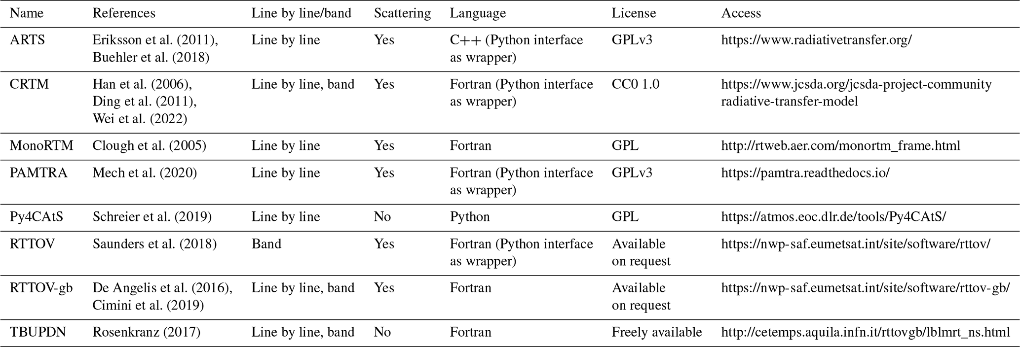
Radiative transfer (RT) models play a fundamental role in atmospheric sciences, as they are broadly used to simulate how electromagnetic radiation travels through the atmosphere as it interacts with atmospheric constituents (such as gases, aerosols, and hydrometeors) through absorption, emission, scattering, and refraction. RT models are commonly used as forward operators to simulate and understand remote sensing observations from any platform, whether ground-based, airborne, or spaceborne. RT calculations depend on the state of the atmosphere (pressure, temperature, composition), the optical properties of the atmospheric constituents (molecules and particles), the simulated observing geometry, and the spectral range. Given a set of specifications on the spectral range, atmospheric conditions, and observing geometry, the RT model is able to compute the atmospheric opacity and the observations simulated accordingly. Simulated observations are then used in a broad range of applications, from atmospheric process understanding and the retrieval of atmospheric variables to data assimilation into numerical weather prediction (NWP) models. Although the theoretical aspects of wave–atmosphere interactions are essentially the same throughout the electromagnetic spectrum, different RT models have been developed to account for the specific features of limited spectral ranges, such as the visible, infrared, and microwave portions of the electromagnetic spectrum. In particular, several microwave (MW) RT models have been developed throughout the years to serve the needs of passive remote sensing from MW radiometers (e.g., Liebe, 1989; Buehler et al., 2005; Rosenkranz, 2017). Many examples are available in the available literature on the use of MW RT models for atmospheric sciences, including but not limited to the following: process understanding (Tripoli et al., 2005; Martinet et al., 2017), atmospheric retrieval development (Eriksson et al., 2005; Boukabara et al., 2013; Sanò et al., 2015; Larosa et al., 2023), MW instrument design and validation (Buehler et al., 2012; Fox et al., 2017), data assimilation into NWP models (Eyre et al., 2020; Martinet et al., 2020), and instrument synergy (Marzano et al., 1999; Turner and Löhnert, 2021; Cimini et al., 2023). A variety of software has been developed throughout the past 3 decades for implementing different flavors of available MW RT models, differing in features, assumptions, and approximations, as well as coding languages. Among the different features, RT codes may be classified as scattering or non-scattering (i.e., considering absorption only). Similarly, RT codes may be classified as line by line, meaning that RT can be modeled at any frequency from the contributions of many gas absorption lines, or parameterized, meaning that RT can be modeled at a limited number of channels for which the optical depth is parameterized considering their spectral response function, initially trained with line-by-line calculations. Other assumptions include the observing geometry, going from one-dimensional (1-D) plane-parallel calculations, considering the atmosphere state changing only in the vertical dimension, to higher-dimensional (2-D or 3-D) geometries, allowing for the consideration of the horizontal spatial inhomogeneity, to spherical geometry, allowing for the proper modeling of the atmospheric shape and its effect on the bending angle of the radiation path. Although RT codes enabling line-by-line, scattering, and spherical geometry computations are much more complex and computationally demanding than the parameterized, non-scattering, and 1-D plane-parallel assumptions, they allow for more accurate modeling of the impact of the spectral resolution, particle size, and 3-D distribution, respectively. Concerning the coding language, most of MW RT software codes are available in compiled programming languages such as C, C$++$, and Fortran. However, the interpreted programming language Python has become increasingly popular for scientific computing in the last decades, thanks to its numerous extension packages, and it is now widely considered the language of choice in many areas, including atmospheric science. Therefore, some of the available RT codes allow users to access their features by running Python modules as wrapper of the core software, although the core software needs to be compiled from source or used in a binary form to access such modules. There are also cases for which the original code has been translated into Python. Table 1 reports a list of most popular MW RT codes, by no means complete, with their key features and access information. In the following, a brief introduction of the most relevant MW RT codes for this paper is given.

Table 1 List of popular codes suitable for atmospheric radiative transfer in the microwave spectral region. CC: Creative Commons, GPL: GNU Public License. Last access: 29 February 2024 (for all links in this table).

ARTS. The Atmospheric Radiative Transfer Simulator (ARTS) is a radiative transfer model suitable for calculations from the microwave to the thermal infrared spectral range (Buehler et al., 2005, 2018; Eriksson et al., 2011). ARTS is implemented in C$++$ with a modular design, allowing for the flexibility to perform many different applications concerning radiative transfer calculations in all viewing geometries from inside or outside the atmosphere: up-looking, down-looking, and limb-looking. ARTS allows for the choice of different state-of-the-art absorption models, including line-by-line calculations from HITRAN (high-resolution transmission molecular absorption database) or other catalogues plus various absorption continuum parameterizations. It is fully polarized, allowing for RT calculations of one to four Stokes components. It allows for scattering computations from spherical and non-spherical atmospheric particles. It also provides analytical or semi-analytical Jacobians for a large set of state parameters. It supports XML and NetCDF (Network Common Data Format) file format for data import and export. ARTS can be run standalone or through external tools, such as PyARTS, a Python package that serves as wrapper for the main ARTS core library. PyARTS is part of the ARTS source repository. PyARTS provides an interactive interface to the ARTS engine for running radiative transfer simulations and has many built-in ARTS types for the manipulation of input data and the evaluation of simulation results. However, PyARTS cannot be run as a standalone Python package as it needs ARTS to be built before.

CRTM. The Community Radiative Transfer Model (CRTM; Han et al., 2006; Ding et al., 2011; Wei et al., 2022) is a fast radiative transfer model developed to efficiently simulate specific spaceborne Earth-observing sensors. CRTM was developed by the US Joint Center for Satellite Data Assimilation (JCSDA) to be a library for users to link to from other models. However, CRTM can be run in standalone mode. CRTM is a sensor-based RT model, supporting more than 100 sensors on meteorological and other remote sensing satellites, covering wavelengths ranging from the visible through the microwave. The source code is written in standard Fortran 95 and makes extensive use of modules and derived data structures. CRTM includes both the forward model and its Jacobian with respect to the input atmospheric-state variables, accounting for the absorption of atmospheric gases as well as the multiple scattering of water and ice clouds composed of a variety of spherical and nonspherical particles, working under all atmospheric and surface conditions. CRTM is extensively used in several applications, such as the NOAA Microwave Integrated Retrieval System (MiRS), the National Centers for Environmental Prediction (NCEP) data assimilation system, and the NOAA STAR (Center for Satellite Applications and Research) Integrated Calibration and Validation System Long-Term Monitoring System. CRTM can be called from Python scripts using pyCRTM, which embeds CRTM Fortran data structures and procedures directly into Python, taking advantage of both the simplicity and ease of use of Python syntax and the flexibility that comes from the extensive Python ecosystem (Karpowicz et al., 2022).

MonoRTM. MonoRTM represents an atmospheric radiative transfer model widely used in the scientific community to generate simulated spectral radiance ranging from the ultraviolet to the microwave region (Clough et al., 2005). It has been produced by Atmospheric and Environmental Research (AER) and is based on the same physical properties and continuum absorption model as the Line-By-Line Radiative Transfer Model (LBLRTM), which is also developed and maintained by AER. These are both Fortran 90 codes; however MonoRTM is particularly suitable to simulate a single or a set of a few monochromatic wavelengths. Atmospheric molecular absorption covers all spectral regions, with molecular optical depths computed within the Monochromatic Optical Depth Model module; however, the spectral-radiance calculation in the presence of cloud liquid water is only possible in the microwave range and relies on the model developed by Liebe et al. (1991). MonoRTM also accounts for molecular absorption within the spectral line center, using the MT_CKD continuum (Clough et al., 2005). Line-coupling effects, which are crucial for, e.g., oxygen lines in the microwave region, are also dealt with in the code (Rosenkranz, 1988; Tretyakov et al., 2005; Cadeddu et al., 2007).

PAMTRA. This is an atmospheric radiative transfer code, namely Passive and Active Microwave radiative TRAnsfer (PAMTRA; Mech et al., 2020), specifically designed to simulate both passive microwave radiances as well as active remote sensing measurements in the presence of cloudy atmosphere. PAMTRA exploits the passive forward model to compute both up- and down-looking polarized brightness temperatures and radiances for the passive part. The active part can simulate the full radar Doppler spectrum and its higher moments (mean Doppler velocity, skewness, kurtosis). The model is built within a Fortran–Python environment, allowing for the flexibility of different input/output (I/O) formats and instrument characteristics (e.g., observations from ground-based, airborne, or spaceborne platforms and viewing angles), with the assumption of a one-dimensional plane-parallel homogeneous atmosphere over the horizontal direction. The user can select several operational modes among scattering and absorption models, within a variety of spectroscopic parameters and databases. The absorption model by Rosenkranz (1998) is used to simulate the atmospheric gas absorption considering later modifications (e.g., Turner et al., 2009). Moreover, PAMTRA implements the self-similar Rayleigh–Gans approximation (SSRGA) for both active and passive applications (Hogan et al., 2017). Generally, pyPAMTRA is used in the scientific community, which features a Python wrapper built around the Fortran core, allowing for direct access from Python, without using the Fortran I/O routines. The pyPAMTRA interface makes the model user-friendly, simplifying the importing of model data, the output in terms of files or plots, and the parallel running of the code on a multicore processor or cluster machines.

Py4CAtS. Python scripts for Computational ATmospheric Spectroscopy (Py4CAtS; Schreier et al., 2019) is a software designed for computing atmospheric spectroscopy both in the infrared and microwave spectral regions. It was initially conceived to enable Python access to the previous Fortran 90 Generic Atmospheric Radiation Line-by-line Code (GARLIC; Schreier et al., 2014). Later on, it has become a complete self-consistent independent software, based entirely on Python numerical array processing modules, providing line-by-line radiances, as well as absorption cross sections and coefficients, optical depths, transmissions, and weighting functions. Py4CAtS consists of a set of modules and functions, allowing for generating line-by-line cross sections for given pressure(s) and temperature(s), to combine cross sections into absorption coefficients and optical depths and to integrate along the line of sight into transmission and radiance/intensity. Py4CAtS is also user-friendly, since it offers an interactive environment and the possibility for performing batch line-by-line modeling. The software can be started within the console terminal, the Python interpreter, or the Jupyter Notebook; moreover, all intermediate variables can be visualized too. Py4CAtS relies on a plane-parallel atmosphere assumption and considers non-scattering interactions, with the Schwarzschild equation featuring thermal emission as the source only; furthermore, neither continuum- nor collision-induced absorptions are taken into account as contributions to the molecular absorption, which is therefore limited to the Voigt line shape. More a recent version of Py4CAtS incorporates continuum-induced absorption; simple single scattering; and modeling of aerosol optical depth and speed dependence of pressure broadening, including line mixing (Schreier, 2017; Schreier and Hochstaffl, 2021).

RTTOV. Similar to CRTM, the Radiative Transfer for TOVS (RTTOV; Television Infrared Observation Satellite (TIROS) Operational Vertical Sounder) is a fast radiative transfer model for modeling passive visible, infrared, and microwave downward-viewing satellite radiometers, spectrometers, and interferometers (Saunders et al., 2018; Hocking et al., 2021). RTTOV is a Fortran 90 code designed to be incorporated within user applications for simulating satellite radiances. RTTOV is developed and maintained by the NWP Satellite Application Facility of EUMETSAT, and it is probably the most used RT code for satellite data assimilation into NWP models. Given an atmospheric profile of temperature; water vapor; and, optionally, trace gases, aerosols, and hydrometeors, together with surface parameters and a viewing geometry, RTTOV computes the top-of-atmosphere radiances for a set of spaceborne sensors from past, current, and future satellite Earth-observing missions. The core of RTTOV is a fast parameterization of layer optical depths due to gas and liquid water absorption. Profiles of layer-to-space transmittances computed by the line-by-line code AMSUTRAN (Turner et al., 2019) are the basis for the training of the fast parameterization in the microwave region. RTTOV consists of both the forward model, which simulates the upwelling radiances for a given sensor, and its Jacobian, which calculates the radiance derivatives with respect to the input atmospheric-state variables. RTTOV includes scattering calculations for simulating cloudy and aerosol-affected radiances in the infrared. Scattering at MW frequencies from hydrometeors of different phases and shapes is available through the wrapper code RTTOV-SCAT (Bauer et al., 2010; Geer et al., 2021). RTTOV has a built-in graphical user interface (GUI) which allows the user to modify an atmospheric/surface profile, run RTTOV for a given instrument, produce radiances and brightness temperatures, calculate Jacobians, perform a basic retrieval, and instantaneously display the results. RTTOV is natively in Fortran, but Python wrappers are available to allow for the functionality of RTTOV in Python. These wrappers provide Python bindings for the RTTOV Fortran code, making it easier for Python users to use. A ground-based version of RTTOV for simulating ground-based MW sensors is also available, though limited to version 11 (De Angelis et al., 2016; Cimini et al., 2019).

TBUPDN. The upward–downward T_B (TBUPDN) code is a library of Fortran routines for the non-scattering line-by-line microwave RT simulations (Rosenkranz, 2017). The code has been developed and maintained by Philip W. Rosenkranz for more than 30 years (Rosenkranz, 1993). TBUPDN is intended as an educational tool with limited ranges of applicability, i.e., calculations of upward- and downward-propagating T_B at the top and bottom of the atmosphere, respectively. The main routines can be run in a standalone mode or read as examples for using the subroutines (e.g., the absorption model routines) in other software programs. A major feature of TBUPDN is the continuous update of absorption routines, originally based on the MPM code, with subsequent spectroscopic modifications from most recent findings from laboratory and field campaign experiments (Rosenkranz, 1988, 1998, 2001, 2005; Rosenkranz and Cimini, 2019; Gallucci et al., 2024). User interfaces are provided for handling I/O text files and produce encapsulated PostScript figures.

Table 1 and the list above are meant to provide an overview of open-access codes that are used extensively by the MW community but do not pretend to be complete. Other codes suitable for atmospheric RT in the MW are available, either openly or commercially, e.g., BTRAM (Chapman et al., 2010) and MODTRAN (Berk et al., 2014). Other RT codes that are available in Python or with a Python interface, although not concerning MW in Earth's atmosphere, include the following: PYDOME (Efremenko et al., 2019) for simulating satellite measurements of reflected and scattered solar radiation in the ultraviolet and visible spectral ranges; Py6S (Wilson, 2013), a Python interface to the 6S RTM (Vermote et al., 1997) designed to simulate solar radiation through atmospheres on Earth and other planets; the pySMARTS module (Ayala Pelaez and Deline, 2020), containing functions for calling SMARTS (Simple Model of the Atmospheric Radiative Transfer of Sunshine) to compute clear-sky spectral irradiances (on a tilted or horizontal receiver plane) for specified atmospheric conditions; petitRADTRANS (Mollière et al., 2019); and PYRATE (Tritsis et al., 2018) for simulating RT through atmospheres on exoplanets.

This paper introduces PyRTlib, a new standalone Python package for non-scattering line-by-line microwave RT simulations. Given the premises above, one may ask the following question: is a new RT code really needed? The intention for PyRTlib is not to be considered a competitor to the codes mentioned above, which represent the cutting edge with their own peculiarities, in terms of efficiency, flexibility, modularity, and applicability. Nevertheless, the reasons behind the development of PyRTlib are the following:

1. to develop an educational tool, similar to TBUPDN but in Python, which nowadays represents the most used language for scientific software development, especially by students and younger scientists;

2. to provide user-friendly Python interfaces, similar to those of PyARTS or pyPAMTRA, to compute MW RT simulations using popular datasets as input, such as a radiosonde repository or global reanalysis;

3. to allow for easy comparison of MW calculations using different atmospheric-absorption models, e.g., those proposed throughout the last 3 decades, for any platform (ground-based, airborne, and spaceborne) and observing geometry (zenith, nadir, slant), except for limb-sounding geometry (not currently implemented in PyRTlib);

4. to provide T_B calculations with the associated uncertainty due to the uncertainty in spectroscopic parameters, following a general rigorous approach that has been recently outlined (Cimini et al., 2018; Gallucci et al., 2024).

In particular, to our knowledge the uncertainty estimate is not available by any other MW RT code, making PyRTlib unique to this aspect in the MW RT scenario. Thus, this paper provides a description of PyRTlib version 1.0 and advocates its use through a range of examples demonstrating its value in producing passive MW simulations from notable input datasets (radiosondes, reanalysis) and for ground-based, airborne, and satellite perspectives.

The paper is structured as follows: a brief introduction on the basics of equations of a radiative transfer model, the main absorption model available, and how profiles can be interpolated and extrapolated is provided in Sect. 2. The tools for retrieving and managing input data from open-access repositories (e.g., radiosonde observations and model reanalysis) are discussed in Sect. 3. Usage of the code, as well as some implementation details and a few examples of applications, is presented in Sect. 4. Section 5 summarizes the conclusions and future developments, while Sect. 6 provides instructions for code availability and usage.

2 Radiative transfer model

An atmospheric RT model simulates the propagation of electromagnetic radiation through the atmosphere as it interacts with atmospheric constituents (gases, aerosols, and hydrometers) through absorption, emission, scattering, and refraction. The intensity of radiation I, also called radiance, expresses the power carried by the electromagnetic radiation along the direction of propagation per unit area and at a solid angle at a given frequency f. Considering an ideal blackbody radiator in local thermodynamic equilibrium at physical temperature T, the intensity of radiation I is given by the Planck function:

$$\begin{array}{}\text{(1)}& B_{\mathrm{f}}\left(T\right)=\left({\displaystyle \frac{\mathrm{2}h{f}^{\mathrm{3}}}{c^{\mathrm{2}}}}\right)\left({\displaystyle \frac{\mathrm{1}}{e^{\frac{hf}{kT}}-\mathrm{1}}}\right),\end{array}$$

where h and k are the Planck and Boltzmann constants, respectively, and c is the speed of light. From Eq. (1) directly comes the definition of brightness temperature T_B, as the temperature that a blackbody radiator should have to emit the radiance I, i.e., I=B_f(T_B).

The relevance of radiation scattering by atmospheric particles depends on the ratio between the size of the scattering particle r and the radiation wavelength λ, the so-called size ratio $x=\mathrm{2}\mathit{\pi }r/\mathit{\lambda }=\mathrm{2}\mathit{\pi }rf/c$ (Petty, 2006). If x≪1, then the contribution of scattering can be considered negligible. That is the case at microwave and millimeter-wave frequencies (1 THz) in clear-sky conditions (no clouds). For relatively small hydrometeors (i.e., liquid and ice clouds) the size ratio is still x<1 and the Rayleigh approximation is valid, for which absorption is still dominant with respect to scattering. Thus, a simplifying common assumption at microwave frequencies is to neglect atmospheric scattering, which is commonly assumed valid in the absence of large particles (i.e., liquid and solid precipitation). In such a case, the Schwarzschild equation applies, i.e.,

$$\begin{array}{}\text{(2)}& \begin{array}{rl}{B}_{\mathrm{f}}\left(T_{\mathrm{B}}\right)& =B_{\mathrm{f}}\left(T_{\mathrm{BG}}\right)e^{-{\mathit{\tau }}_f(\mathrm{0},\mathrm{\infty })}+\underset{\mathrm{0}}{\overset{\mathrm{\infty }}{\int }}{B}_{\mathrm{f}}\left(T\right(s\left)\right){\mathit{\alpha }}_f\left(s\right)\\ & e^{-{\mathit{\tau }}_f(\mathrm{0},s)}\mathrm{d}s,\end{array}\end{array}$$

where s indicates the distance from the observations point along the line of sight, α_f indicates the atmospheric-absorption coefficient, τ_f indicates the atmospheric opacity (${\mathit{\tau }}_f\left(ab\right)={\int }_a^b{\mathit{\alpha }}_f\left(s\right)\mathrm{d}s$), and the two extremes of the integral indicate the position where the T_B measurement is taken (0) and the position of a uniform background of temperature T_BG (∞). The first term of Eq. (2) changes depending on the observing geometry. For an up-looking radiometer measuring downwelling radiation, without discrete sources (such as the Sun or Moon) within the antenna field of view, B_f(T_BG) is simply equal to B_f(T_CBG), where T_CBG≃2.7 K is the microwave cosmic background brightness temperature (Rosenkranz, 1993). For a down-looking radiometer measuring upwelling radiation, e.g., from a satellite platform, a typical background is Earth's surface, the spectral emissivity (ε_f) of which must be taken into account to model the complementary contribution of Earth's surface emission and reflection of downwelling radiation. Thus, indicating with SRF the position of Earth's surface and TOA the top of the atmosphere, B_f(T_BG) in Eq. (2) becomes

$$\begin{array}{}\text{(3)}& \begin{array}{rl}{B}_{\mathrm{f}}\left(T_{\mathrm{BG}}\right)& =(\mathrm{1}-{\mathit{\epsilon }}_f)\left[B_{\mathrm{f}}\left(T_{\mathrm{CBG}}\right)e^{-{\mathit{\tau }}_f(\mathrm{SRF},\mathrm{TOA})}\right.\\ & \left.+\underset{\mathrm{SRF}}{\overset{\mathrm{TOA}}{\int }}{B}_{\mathrm{f}}\left(T\right(s\left)\right){\mathit{\alpha }}_f\left(s\right)e^{-{\mathit{\tau }}_f(SRF,s)}\mathrm{d}s\right]\\ & +{\mathit{\epsilon }}_f{B}_{\mathrm{f}}\left(T_{\mathrm{SRF}}\right).\end{array}\end{array}$$

The integral in the atmospheric terms in Eqs. (2) and (3) is divided into the sum of integrals over each of the NL-1 (number of level profiles) layers in between the NL levels in which the atmosphere is discretized (Schroeder and Westwater, 1991). In the case of up-looking simulations of downwelling radiation:

$$\begin{array}{}\text{(4)}& \begin{array}{rl}\underset{\mathrm{0}}{\overset{\mathrm{\infty }}{\int }}& B_{\mathrm{f}}\left(T\right(s\left)\right){\mathit{\alpha }}_f\left(s\right)e^{-{\mathit{\tau }}_f(\mathrm{0},s)}\mathrm{d}s\cong {\sum }_{i=\mathrm{2}}^{\mathrm{NL}}\\ & \underset{s_{i-\mathrm{1}}}{\overset{s_i}{\int }}{B}_{\mathrm{f}}\left(T\right(s\left)\right){\mathit{\alpha }}_f\left(s\right)e^{-{\mathit{\tau }}_f(\mathrm{0},s)}\mathrm{d}s.\end{array}\end{array}$$

The integrals in the second term can be simplified by introducing a mean radiating temperature of a layer T_MR, such as

$$\begin{array}{}\text{(5)}& \begin{array}{rl}\underset{s_{i-\mathrm{1}}}{\int }{s}_i& B_{\mathrm{f}}\left(T\right(s\left)\right){\mathit{\alpha }}_f\left(s\right)e^{-{\mathit{\tau }}_f(\mathrm{0},s)}\mathrm{d}s=B_{\mathrm{f}}\left(T_{\mathrm{MR}}\right)\\ & \underset{s_{i-\mathrm{1}}}{\overset{s_i}{\int }}{\mathit{\alpha }}_f\left(s\right)e^{-{\mathit{\tau }}_f(\mathrm{0},s)}\mathrm{d}s=B_{\mathrm{f}}\left(T_{\mathrm{MR}}\right)e^{-{\mathit{\tau }}_f(\mathrm{0},s_{i-\mathrm{1}})}\\ & \left[\mathrm{1}-e^{-{\mathit{\tau }}_f(s_{i-\mathrm{1}},s_i)}\right],\end{array}\end{array}$$

where B_f(T_MR) for the layer of atmosphere between a and b is defined as

$$\begin{array}{}\text{(6)}& B_{\mathrm{f}}\left(T_{\mathrm{MR}}\right)={\displaystyle \frac{{\int }_a^b{B}_{\mathrm{f}}\left(T\left(s\right)\right){\mathit{\alpha }}_f\left(s\right)e^{-{\mathit{\tau }}_f\left(\mathrm{0},s\right)}\mathrm{d}s}{e^{-{\mathit{\tau }}_f\left(\mathrm{0},a\right)}\left[\mathrm{1}-e^{-{\mathit{\tau }}_f\left(a,b\right)}\right]}},\end{array}$$

where B_f(T_MR) can be approximated as the weighted average of B_f(T(s)) from the two profile levels that form the layer

$$\begin{array}{}\text{(7)}& B_{\mathrm{f}}\left(T_{\mathrm{MR}}\right)\simeq {\displaystyle \frac{B_{\mathrm{f}}\left(T\right(s_{i-\mathrm{1}}\left)\right)+B_{\mathrm{f}}\left(T\right(s_i\left)\right)e^{-{\mathit{\tau }}_f(s_{i-\mathrm{1}},s_i)}}{\mathrm{1}+e^{-{\mathit{\tau }}_f(s_{i-\mathrm{1}},s_i)}}},\end{array}$$

where the exponential weight $e^{-{\mathit{\tau }}_f(s_{i-\mathrm{1}},s_i)}$ represents the attenuation of B_f(T(s_i)) over the layer between levels i and i−1. Note that introducing the layer transmittance $T=e^{-{\mathit{\tau }}_f(s_{i-\mathrm{1}},s_i)}$ in Eq. (7), it becomes

$$\begin{array}{}\text{(8)}& B_{\mathrm{f}}\left(T_{\mathrm{MR}}\right)\simeq {\displaystyle \frac{B_{\mathrm{f}}\left(T\right(s_{i-\mathrm{1}}\left)\right)+B_{\mathrm{f}}\left(T\right(s_i\left)\right)T}{\mathrm{1}+T}}.\end{array}$$

Thus, B_f(T_MR) is the average brightness temperatures at the layer boundaries, weighted by the layer transmittance, going from B_f(T(s_i−1)) to $\frac{B_{\mathrm{f}}\left(T\right(s_{i-\mathrm{1}}\left)\right)+B_{\mathrm{f}}\left(T\right(s_i\left)\right)}{\mathrm{2}}$ as the layer gets from totally opaque (T=0) to totally transparent (T=1). Other weighting options, such as the so-called linear in tau, are used elsewhere (Saunders et al., 2018). The contribution of each layer is then summed up as in Eq. (4) (Schroeder and Westwater, 1991). The case of down-looking observations can be simply derived from the equations above.

2.1 Modeling atmospheric absorption

Modeling atmospheric absorption is a crucial component of RT codes. Absorption models are based on parameterized equations to calculate atmospheric absorption (α_f in Eq. 2) given the constituents' concentration and their thermodynamic conditions (Rosenkranz, 1993). Note that, as introduced earlier, PyRTlib is a non-scattering RT code; i.e., it assumes that attenuation is due entirely to absorption by atmospheric gases and cloud water, while it neglects the extinction due to particle scattering. Concerning atmospheric gases, PyRTlib considers the absorption contribution by nitrogen and oxygen (also called dry-air contribution, α_dry) and water vapor (wet contribution, α_wet). These three species sum up to more than 99 % of the atmospheric gas mixture and account for most of the gas absorption in the MW spectrum. In general, the gas absorption is expressed as the sum of a resonant component (due to absorption lines of individual molecules) and a non-resonant component (due to the interaction between molecules): ${\mathit{\alpha }}_{\mathrm{total}}={\mathit{\alpha }}_{\mathrm{res}}+{\mathit{\alpha }}_{\mathrm{nr}}$. The resonant absorption is modeled by computing the contribution of each significant absorption line (line by line) so that for a specified molecular species with n molecules per unit volume the power absorption coefficient at frequency ν is given by

$$\begin{array}{}\text{(9)}& {\mathit{\alpha }}_{\mathrm{res}}=\sum _i{\mathit{\alpha }}_{\mathrm{line}}(\mathit{\nu },{\mathit{\nu }}_i)=n\sum _i{S}_i\left(T\right)F(\mathit{\nu },{\mathit{\nu }}_i),\end{array}$$

where k is the Boltzmann constant and E_low is the energy of the lower level of

$$\begin{array}{}\text{(10)}& S_i\left(T\right)=S_i\left(T_{\mathrm{0}}\right){\mathit{\theta }}^{n_S}\exp \left({\displaystyle \frac{E_{\mathrm{low}}+h{\mathit{\nu }}_i/\mathrm{2}}{k{T}_{\mathrm{0}}}}\left(\mathrm{1}-\mathit{\theta }\right)\right),\end{array}$$

with the line intensity at temperature T, which, with respect to its value at the reference temperature T₀, depends on the so-called inverse temperature $\mathit{\theta }=\frac{T_{\mathrm{0}}}{T}$ and the temperature exponent n_S, and

$$\begin{array}{}\text{(11)}& \begin{array}{rl}F\left(\mathit{\nu },{\mathit{\nu }}_i\right)& ={\displaystyle \frac{\mathrm{1}}{\mathit{\pi }}}{\left({\displaystyle \frac{\mathit{\nu }}{{\mathit{\nu }}_i}}\right)}^{\mathrm{2}}\left[{\displaystyle \frac{\mathrm{\Delta }{\mathit{\nu }}_i+Y_i\cdot \left(\mathit{\nu }-{\mathit{\nu }}_i\right)}{\mathrm{\Delta }{\mathit{\nu }}_i^{\mathrm{2}}+{\left(\mathit{\nu }-{\mathit{\nu }}_i\right)}^{\mathrm{2}}}}\right.\\ & \left.+{\displaystyle \frac{\mathrm{\Delta }{\mathit{\nu }}_i-Y_i\cdot \left(\mathit{\nu }+{\mathit{\nu }}_i\right)}{\mathrm{\Delta }{\mathit{\nu }}_i^{\mathrm{2}}+{\left(\mathit{\nu }+{\mathit{\nu }}_i\right)}^{\mathrm{2}}}}\right]\end{array}\end{array}$$

is the line-shape function of the ith absorption line at center frequency ν_i, with the half width at half amplitude Δν_i, and mixing parameter Y_i, which all have some dependence on temperature and/or pressure (Rosenkranz, 1993; Cimini et al., 2018). Conversely, the non-resonant absorption is characterized by smooth frequency dependence. The dry-air contribution is modeled through a frequency-dependent factor f(ν) to fit experimental data as ${\mathit{\alpha }}_{\mathrm{nr}\mathrm{\_}\mathrm{dry}}\left(\mathit{\nu },T\right)=C_{\mathrm{d}}f\left(\mathit{\nu }\right){\mathit{\theta }}^{n_{\mathrm{d}}}{P}_{\mathrm{d}}^{\mathrm{2}}{\mathit{\nu }}^{\mathrm{2}}$, where C_d is the intensity coefficient, n_d is the relative temperature-dependence exponent, and P_d is the partial pressures of dry air. Similarly, the non-resonant water vapor absorption is modeled through the contribution of two terms corresponding to the interaction of water molecules with each other (self component) and between water molecules and air molecules (foreign component): ${\mathit{\alpha }}_{\mathrm{nr}\mathrm{\_}\mathrm{wv}}\left(\mathit{\nu },T\right)=\left(C_{\mathrm{s}}{\mathit{\theta }}^{n_{\mathrm{cs}}+\mathrm{3}}{P}_{\mathrm{w}}^{\mathrm{2}}+C_{\mathrm{f}}{\mathit{\theta }}^{n_{\mathrm{cf}}+\mathrm{3}}{P}_{\mathrm{d}}{P}_{\mathrm{w}}\right)\cdot {\mathit{\nu }}^{\mathrm{2}}$, where P_w is the partial pressures of water vapor, while C_s and C_f are empirical intensity coefficients for self- and foreign-induced absorption with their respective temperature-dependence exponents (n_cs, n_cf), respectively. PyRTlib also offers the option to add the contribution of ozone (${\mathit{\alpha }}_{{\mathrm{O}}_{\mathrm{3}}}$); this causes a relatively small absorption increase in very narrow spectral ranges due to many nearly monochromatic spectral lines at the expense of slower computations. Concerning hydrometeors, the absorption of cloud liquid (α_liq) and ice (α_ice) particles are considered, assuming the Rayleigh absorption approximation of Mie forward-scattering theory. This allows for expressing the cloud absorption as a simple function of the complex dielectric constant of liquid (ε_liq) and ice (ε_ice) water, e.g.,

$$\begin{array}{}\text{(12)}& {\displaystyle }{\mathit{\alpha }}_{\mathrm{liq}}=C_{\mathrm{liq}}L\mathit{\nu }I\left(\right({\mathit{\epsilon }}_{\mathrm{liq}}-\mathrm{1})/({\mathit{\epsilon }}_{\mathrm{liq}}+\mathrm{2}\left)\right),\text{(13)}& {\displaystyle }{\mathit{\alpha }}_{\mathrm{ice}}=C_{\mathrm{ice}}I\mathit{\nu }I\left(\right({\mathit{\epsilon }}_{\mathrm{ice}}-\mathrm{1})/({\mathit{\epsilon }}_{\mathrm{ice}}+\mathrm{2}\left)\right),\end{array}$$

where I indicates the imaginary part and C_liq and C_liq are constants, while L and I are the liquid and ice water mass content per unit of air volume, respectively. Note that α_dry, α_wet, ${\mathit{\alpha }}_{{\mathrm{O}}_{\mathrm{3}}}$, α_liq, and α_ice all depend on the frequency and location in space, although these are not shown for simplicity. In fact, the sum of ${\mathit{\alpha }}_{\mathrm{dry}}+{\mathit{\alpha }}_{\mathrm{wet}}+{\mathit{\alpha }}_{{\mathrm{O}}_{\mathrm{3}}}+{\mathit{\alpha }}_{\mathrm{liq}}+{\mathit{\alpha }}_{\mathrm{ice}}$ represents α_f(s) in Eqs. (2) and (3). Of course, the terms α_liq and α_ice are 0 in clear-sky conditions, while ${\mathit{\alpha }}_{{\mathrm{O}}_{\mathrm{3}}}$ is 0 if the ozone contribution is neglected. Absorption models for computing α_dry, α_wet, ${\mathit{\alpha }}_{{\mathrm{O}}_{\mathrm{3}}}$, α_liq, and α_ice from the constituents' concentration and the thermodynamic conditions are available in the available literature (e.g., Rosenkranz, 1993). These models rely on parameterized equations and spectroscopic parameters, valid up to 1 THz, determined through theoretical calculations and/or laboratory and field measurements. These settings are continuously updated and improved (Liebe et al., 1989; Rosenkranz, 1998; Liljegren et al., 2005; Turner et al., 2009; Mlawer et al., 2012; Koshelev et al., 2018). The proposed changes are occasionally summarized in review articles (e.g., Rothman et al., 2005; Gordon et al., 2017; Rosenkranz, 1998; 2017; Tretyakov, 2016). In particular, PyRTlib implements absorption routines originally based on the MPM code (Liebe, 1989), with subsequent spectroscopic modifications from laboratory and field campaign experiments (Rosenkranz, 1988, 1998, 2005, 2015, 2017; Rosenkranz and Cimini, 2019; Koshelev et al., 2021, 2022). These changes have been summarized in two papers (Cimini et al., 2018; Gallucci et al., 2024). PyRTlib provides the possibility for easily comparing different absorption model configurations, as discussed in one of the examples in Sect. 4. In the case that the input profile contains non-zero cloud liquid and/or ice water, the relative absorption is computed and added to the total absorption. The cloud absorption model used here assumes the Rayleigh approximation, under which scattering is negligible relative to absorption and absorption is independent of cloud particle size distribution. These assumptions restrict the model to non-precipitating clouds with particle radii less than about 100 µm for a frequency less than 100 GHz. Therefore, in its current version, PyRTlib is not adequate for modeling extinction by rain or large cloud droplets or ice particles. Absorption by cloud ice (α_ice) particles is implemented following the algorithms described in Schroeder and Westwater (1991). More than one model are implemented for the absorption by cloud liquid (α_liq) particles, i.e., the one from Liebe et al. (1991) and later improvements (i.e., Liebe et al., 1993). Another model, as in Rosenkranz (2015), is also implemented. This model was developed to be applicable up to 60 °C, but it is specifically recommended for temperatures as low as −25 °C for modeling the absorption of supercooled liquid water particles. Therefore, three models for liquid cloud absorption are currently available within PyRTlib and can be alternatively selected by the user.

2.2 Modeling a continuous atmosphere

To compute absorption throughout the atmosphere, the gas concentrations and thermodynamic profiles are to be provided as input. While O₂ concentration is assumed constant with altitude, the concentration of H₂O (and O₃ if considered) is usually variable with altitude, and this is similar for air pressure and temperature. These inputs may come from atmospheric measurements (e.g., balloon-borne radiosoundings) or atmospheric model output (e.g., NWP model) and are typically available at discrete levels. To compute realistic simulated observations from ground-based or satellite platforms, the profiles must cover the vertical range from Earth's surface to a reasonable top of the atmosphere (TOA), where the atmosphere is so limited that it negligibly affects MW radiation. In practice, the TOA is assumed to approximate the infinite limits on the integral in Eq. (2). For simulations of downwelling radiation, the vertical range could be reduced at the bottom to the height of the simulated receiving antenna (e.g., for the simulations of airborne or elevated instruments). PyRTlib provides functions to extend the input profile to a TOA at 0.1 mbar (following Schroeder and Westwater, 1991), a pressure well below the minimum pressure (i.e., maximum altitude) reached by radiosoundings. This profile extension follows a recommendation (ITU-R P.835-6, 2017) by the International Telecommunication Union – Radiocommunication Sector (ITU-R), providing expressions and data for reference standard atmospheres required for the calculation of gaseous attenuation on Earth–space paths. In particular, PyRTlib currently implements the data in Annex 1, i.e., standard atmospheres to be used to determine temperature, pressure, and water vapor pressure as a function of altitude, when more reliable local data are not available. Data in Annex 3, i.e., providing vertical profiles capturing diurnal, monthly, and seasonal variations from ECMWF 15-year dataset reanalysis (ERA-15) will be implemented in future PyRTlib releases. Another option is to increase the level density by adding levels through interpolation. This option allows for a maximum pressure difference between a pair of adjacent profile levels. If the pressure difference in the input profile exceeds the specified maximum value, PyRTlib divides the layer between the two levels into the smallest number of equally spaced pressure levels that differ by less than the specified maximum value, using linear interpolation in a natural logarithm of pressure.

2.3 Modeling observation geometry

The input height profile h is assumed to represent the vertical line-of-sight ray path coordinate. This corresponds to s in Eq. (2) for up-looking zenith-pointing simulations and to h_TOA−s for down-looking nadir-pointing simulations. For observing angles different from zenith or nadir, the ray path increases due to the slant path through the atmosphere. Considering a plane-parallel atmosphere, the increase effectively corresponds to the multiplicative factor secantϕ, where ϕ is angle with respect to zenith/nadir (or cosecantθ if the elevation angle θ is considered). This approximation only requires the elevation angle θ and the profile of the atmospheric thermodynamical status (pressure, temperature, relative humidity, cloud water content) as a function of altitude over Earth's surface (h), and it is the default option in PyRTlib. A one-dimensional spherical atmosphere can also be considered, which assumes the atmosphere as uniform concentric layers around a smooth spherical Earth. Following Schroeder and Westwater (1991), the ray path for a spherically stratified atmosphere is modeled through Snell's law for polar coordinates:

$$\begin{array}{}\text{(14)}& nr\cos \mathit{\theta }=\mathrm{constant},\end{array}$$

where n is the atmospheric refractive index and r is the radial distance from the center of Earth to a point on the ray path. All these qualities depend only on height above the surface. The radiance distance r is assumed to be Earth's geoid radius (R_E) plus the height above the surface. Note that the constant in Eq. (14) must be set in one point of the ray path. This is currently set at the lowest available atmospheric level, which imposes the limitation that PyRTlib version 1.0 cannot simulate limb-sounding observations. The refractive index n is computed from the dry and wet refractivity (N_d and N_w, respectively) and the inverse compressibility of dry air and water vapor ($Z_{\mathrm{d}}^{-\mathrm{1}}$ and $Z_{\mathrm{w}}^{-\mathrm{1}}$, respectively) through the following non-dispersive model:

$$\begin{array}{}\text{(15)}& {\displaystyle }n=\mathrm{1}+\left(N_{\mathrm{d}}+N_{\mathrm{w}}\right)\cdot {\mathrm{10}}^{-\mathrm{6}},\text{(16)}& {\displaystyle }{N}_{\mathrm{d}}=k_{\mathrm{1}}\left({\displaystyle \frac{P_{\mathrm{d}}}{T}}\right)Z_{\mathrm{d}}^{-\mathrm{1}},\text{(17)}& {\displaystyle }{N}_{\mathrm{w}}=\left(k_{\mathrm{2}}{\displaystyle \frac{e}{T}}+k_{\mathrm{3}}{\displaystyle \frac{e}{T^{\mathrm{2}}}}\right)Z_{\mathrm{w}}^{-\mathrm{1}},\text{(18)}& {\displaystyle }\begin{array}{rl}{Z}_{\mathrm{d}}^{-\mathrm{1}}& =\mathrm{1}+P_{\mathrm{d}}\left(\mathrm{57.90}\cdot {\mathrm{10}}^{-\mathrm{8}}\left(\mathrm{1}+{\displaystyle \frac{\mathrm{0.52}}{T}}\right)-\mathrm{9.4611}\right.\\ & \left.\times {\mathrm{10}}^{-\mathrm{4}}{\displaystyle \frac{T-\mathrm{273.16}}{T^{\mathrm{2}}}}\right),\end{array}\text{(19)}& {\displaystyle }\begin{array}{rl}{Z}_{\mathrm{w}}^{-\mathrm{1}}& =\mathrm{1}+\mathrm{1650}{\displaystyle \frac{e}{T^{\mathrm{3}}}}\left(\mathrm{1}-\mathrm{0.01317}{T}_{\mathrm{C}}+\mathrm{1.75}\times {\mathrm{10}}^{-\mathrm{4}}\right.\\ & \left.T_{\mathrm{C}}^{\mathrm{2}}+\mathrm{1.44}\cdot {\mathrm{10}}^{-\mathrm{6}}{T}_{\mathrm{C}}^{\mathrm{3}}\right),\end{array}\end{array}$$

where T, e, and P_d are the air temperature (K), water vapor partial pressure, and dry-air partial pressure (hPa), respectively, while T_C is the air temperature (°C; $T_{\mathrm{C}}=T-\mathrm{273.16}$). The three k coefficients ($k_{\mathrm{1}}=\mathrm{77.604},k_{\mathrm{2}}=\mathrm{64.79},k_{\mathrm{3}}=\mathrm{3.776}\times {\mathrm{10}}^{\mathrm{5}}$) are given by Saastamoinen (1972) and references therein. PyRTlib optionally provides a slightly modified definition for computing the dry and wet refractivity terms, while leaving the total refractivity and the refractive index unaffected, which is commonly used in geodesy (ESA TN, 2019). Finally, for each specified observing angle a ray-tracing algorithm based on Eq. (14) is used to compute the refracted path length between each pair of adjacent profile levels. The integrals along the ray path are computed assuming that the integrand variable decays exponentially with height within the layer defined by a pair of adjacent levels. With this assumption, the integral along one layer of a general integrand variable X is given by (Schroeder and Westwater, 1991)

$$\begin{array}{}\text{(20)}& \begin{array}{rl}\underset{i-\mathrm{1}}{\overset{i}{\int }}X\left(s\right)\mathrm{d}s& =(s_i-s_{i-\mathrm{1}})\left[\left(X\left(s_i\right)-X\left(s_{i-\mathrm{1}}\right)\right)/\right.\\ & \left.\ln \left(X\left(s_i\right)/X\left(s_{i-\mathrm{1}}\right)\right)\right].\end{array}\end{array}$$

This is used to compute path-integrated quantities, such as layer-integrated absorption profiles for RT calculations as well as total integrals along the entire path, such as the precipitable water vapor; path delay (excess path length) due to dry air and water vapor; and total absorption due to water vapor, dry air, and cloud liquid/ice.

3 Tools for retrieving input data

PyRTlib comes with a built-in module to easily retrieve meteorological data that can be used as input for the RT calculations. These modules allow for easy access to data repositories of radiosonde observations (RAOBs) and model reanalysis. The RAOBs currently considered in PyRTlib are the University of Wyoming Upper Air Data archive and the US National Center for Environmental Information (NCEI) Integrated Global Radiosonde Archive (IGRA) version 2 (Durre et al., 2016). These datasets are retrieved using part of the Siphon (https://github.com/Unidata/siphon, last access: 29 February 2024) library from Unidata. Concerning model reanalysis, PyRTlib currently considers the fifth-generation ECMWF reanalysis (ERA5) as accessible from the Climate Data Store application program interface (CDS API) (https://github.com/ecmwf/cdsapi, last access: 29 February 2024) service. The following subsections describe how the above datasets can be accessed through PyRTlib.

3.1 Radiosondes

Balloon-borne measurements from radiosondes provide accurate, high-resolution profiles of temperature, humidity, and wind from the altitude of the launching site up to the altitude where the balloon bursts (∼30 km for a successful launch). This information is an important piece of the global observing system, and it is widely used in atmospheric research and related services, such as operational meteorology, air quality forecast, climatology, NWP validation and data assimilation, and finally the calibration and validation of remote sensing observations. The University of Wyoming Upper Air Data archive consists of radiosonde balloons from more than 628 globally distributed stations. The data are available at synoptic hours (00, 06, 12, 18 UTC) starting from 1973. The available variables are the latitude, longitude, and elevation of each launching station and the atmospheric profiles of pressure, geopotential height, temperature, dew point temperature, frost point temperature, relative humidity, relative humidity with respect to ice, water vapor mixing ratio, wind direction, wind speed, potential temperature, equivalent potential temperature, and virtual potential temperature. The vertical resolution varies from tens of meters in the lower layers to hundreds of meters near the tropopause, changing according to the site and weather conditions. Listing 1 shows the code to retrieve and plot data measured by one radiosonde launched at 12:00 UTC on 22 April 2021 from the LIRE station (Pratica di Mare Airport, Italy), leading to the graphic output in Fig. 1. Data from any other station available on the University of Wyoming Upper Air Data archive can be accessed knowing the station name or number that can be found through their web interface (https://weather.uwyo.edu/upperair/sounding.html, last access: 29 February 2024).

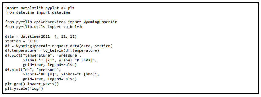
Listing 1 Example code using the PyRTlib module to retrieve radiosonde data from the University of Wyoming Upper Air Data archive.

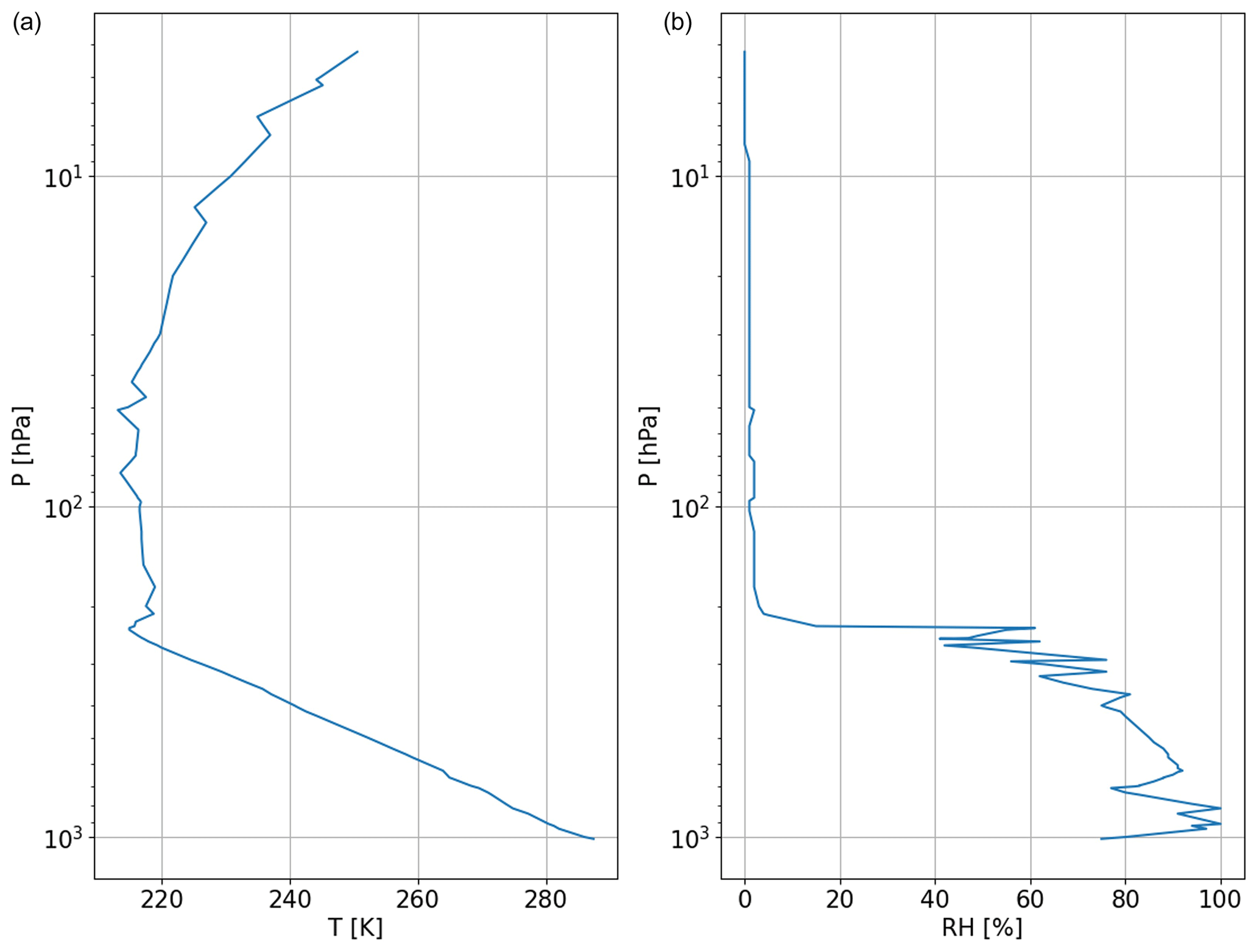
Figure 1 Graphical output of Listing 1, showing atmospheric profiles measured by the radiosonde launched at 12:00 UTC on 22 April 2021 from the LIRE station (Pratica di Mare, Italy). (a) Temperature profile (K). (b) Relative humidity (%).

Another well-known repository for radiosonde data is the Integrated Global Radiosonde Archive (IGRA), consisting of radiosonde and pilot balloon observations from more than 2800 stations distributed globally. The earliest data date back to 1905, and recent data become available in near real time from around 800 stations all over the world. The recording period and temporal and vertical resolution for each station vary over time. Observations are available at standard and variable pressure levels and fixed and variable height wind levels for the surface and tropopause. Variables include time since launch and profiles of atmospheric pressure, temperature, geopotential height, dew point depression, and wind direction and speed at a variable number of levels, including surface, tropopause, and mandatory standard and optional significant levels. The data are released after a quality assurance algorithm performed by the archiving system, checking for format problems, physically implausible values, internal inconsistencies among variables, climatological outliers, and temporal and vertical inconsistencies (Durre et al., 2016, 2018). The IGRA is accessible through NCEI, which also provides access to IGRA station metadata, including information about changes in the station's location, instrumentation, and observation practices over time, which may be useful for interpreting the data. Listing 2 shows the code to retrieve and plot data measured by one radiosonde launched at 12:00 UTC on 22 June 2022 from the station with the network ID of SPM00060018 (Tenerife, Spain), leading to the graphic output in Fig. 2. Data from any other station available on the IGRA can be accessed knowing the station network ID that can be found through their web interface (https://www.ncei.noaa.gov/data/integrated-global-radiosonde-archive/doc/igra2-station-list.txt, last access: 29 February 2024). Note that PyRTlib provides tools to convert atmospheric moisture variables to the standard input relative humidity (e.g., in the given example, the function dewpoint2rh computes relative humidity from dew point depression and physical temperature). PyRTlib then internally computes water vapor pressure and density from temperature and relative humidity using the Goff–Gratch formulas for saturation vapor pressure over liquid and ice water, according to a user-specified switch that determines whether the saturation vapor pressure is calculated over water throughout the profile or over ice when the temperature is below a given threshold.

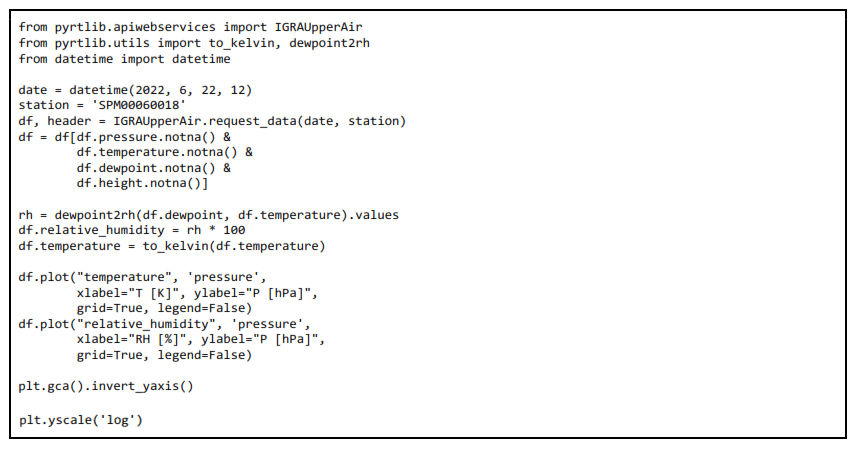
Listing 2 Example code using the PyRTlib module to retrieve radiosonde data from the IGRA 2 archive.

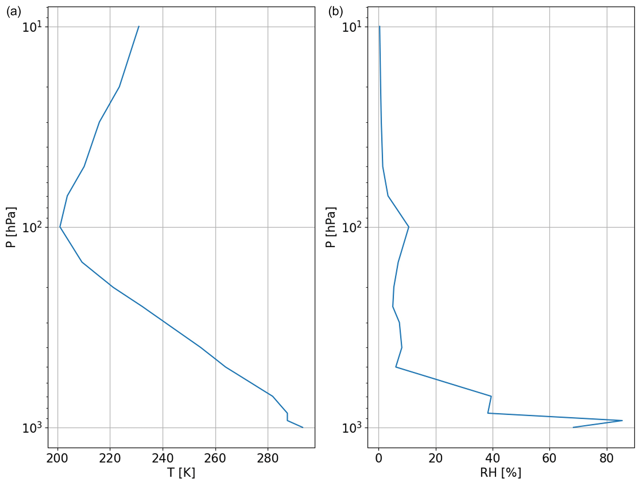
Figure 2 Graphical output of Listing 2, showing atmospheric profiles measured by the radiosonde launched at 12:00 UTC on 22 June 2022 from station SPM00060018 (Tenerife, Spain). (a) Temperature profile (K). (b) Relative humidity (%).

3.2 Model reanalysis

Model reanalysis is an optimal combination of past observations with atmospheric models to provide the most accurate representation of the status of the atmosphere at sub-daily intervals on a regular 3-D spatial grid. In short, forecast models and 4-D data assimilation systems are used periodically to “reanalyze” archived observations based on the variational optimal estimation method. Model reanalysis has substantially evolved during recent decades in generating a consistent time series of multiple climate variables and is nowadays among the most-used datasets in geophysical sciences. ERA5 is the fifth and latest generation of global climate reanalysis produced by ECMWF, providing hourly data of many atmospheric, land-surface, and sea-state parameters together with estimates of uncertainty. ERA5 is based on the most recent and advanced version of the ECMWF Integrated Forecasting System (IFS) model and significantly improved compared to its predecessors (Hersbach et al., 2020). ERA5 is produced and continuously updated by the Copernicus Climate Change Service (C3S) and made available through the Climate Data Store (CDS). ERA5 data are archived on a reduced Gaussian grid, which has quasi-uniform spacing over the globe, at a native resolution of 0.28125° (31 km), from the surface up to about 80 km height. Data can be accessed as either GRIB (GRidded BInary; native) or NetCDF files. PyRTlib implements data retrieval in NetCDF, which is automatically converted and interpolated from the native grids to a regular latitude–longitude grid (0.125°×0.125° grid, i.e., ∼16 km at the Equator) at 37 pressure levels. Hourly estimates of a large number of gridded atmospheric, land, and oceanic climate variables are included from 1979 onwards, with a 5 d delay from real time. Among the available variables the following are selected as input for PyRTlib: temperature, relative humidity, specific cloud ice water content, specific cloud liquid water content, and ozone mass mixing ratio. Listing 3 shows the code to retrieve ERA5 data from the Copernicus CDS for the nearest grid point to a location in southern Italy (lat 39.44°, long 16.04°) on 16 May 2023 at 18:00 UTC. Listing 3 also shows tools to convert the native units for cloud water variables (mass mixing ratios, kg kg⁻¹) in liquid and ice water density (g m⁻³) and plots the cloud liquid water content (CLWC), cloud ice water content (CIWC), and ozone mass mixing ratio (Fig. 3). Data from any other location worldwide from 1979 onwards with a 5 d delay from real time can be accessed by simply providing the longitude, latitude, date, and hour. Note that to access the ERA5 dataset requires configuring an API key. Step-by-step instructions on creating an API key are available at https://cds.climate.copernicus.eu/api-how-to (last access: 29 February 2024).

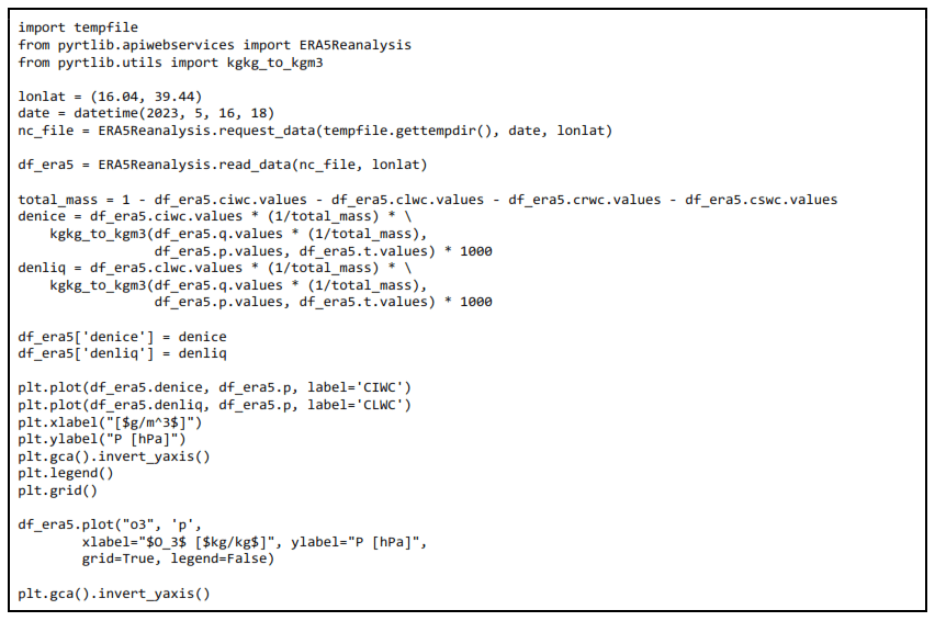
Listing 3 Example code using the PyRTlib module to retrieve atmospheric profiles from the ERA5 reanalysis.

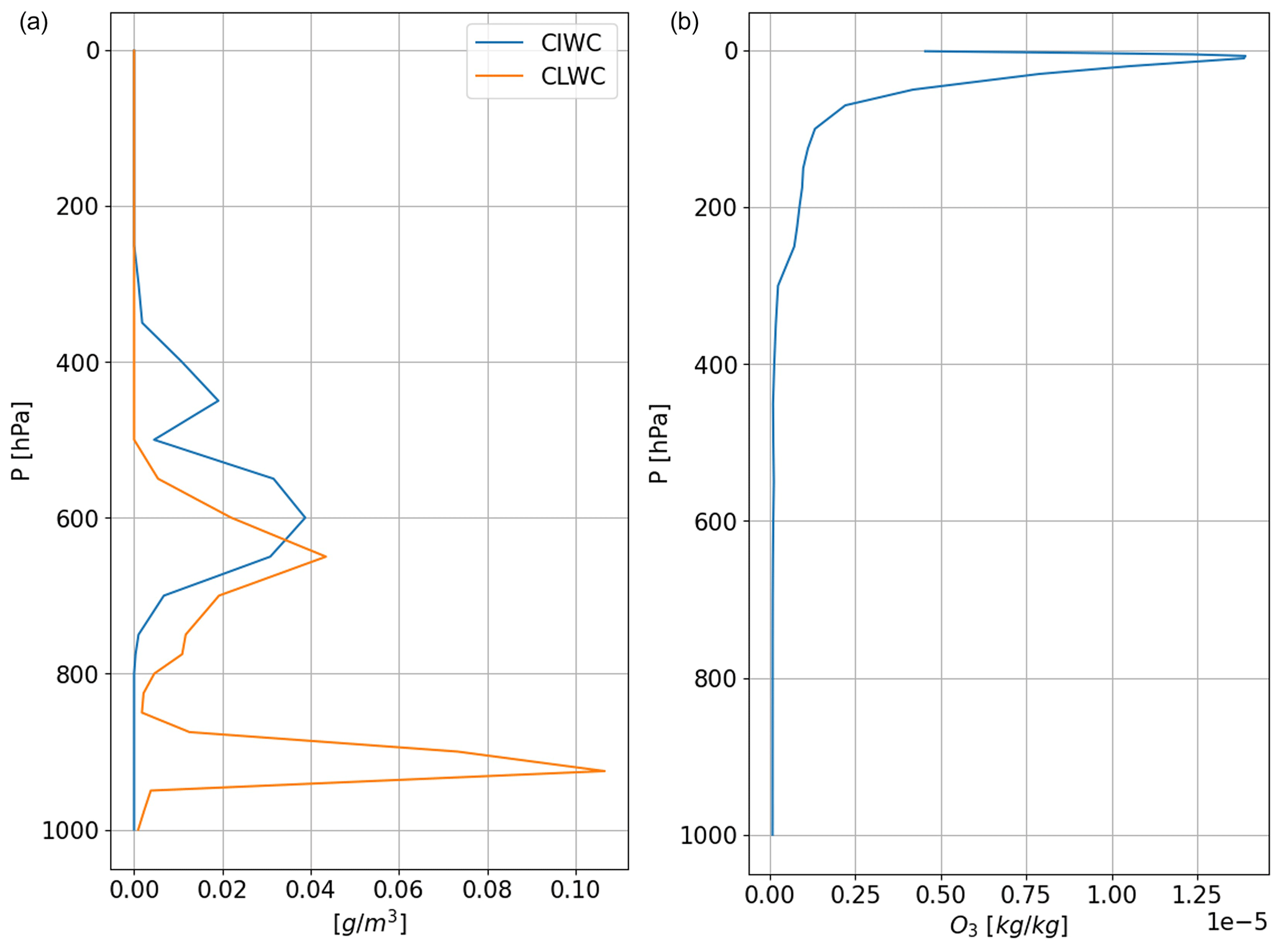
Figure 3 Graphical output of Listing 3, showing atmospheric profiles from the ERA5 reanalysis for the nearest grid point to a location in southern Italy (lat 39.44°, long 16.04°) on 16 May 2023 at 18:00 UTC. (a) Cloud liquid water content (CLWC) and cloud ice water content (CIWC). (b) Ozone mass mixing ratio.

4 Examples of applications

PyRTlib was developed to provide educational RT software in Python, specifically targeting students and younger scientists that mostly use this language for scientific-code development. For this reason, PyRTlib was built with additional modules for facilitating the retrieval and management of popular datasets as input, such as a radiosonde repository or global reanalysis, as shown in Sect. 3. This makes PyRTlib a useful end-to-end RT tool for pedagogical purposes, being flexible and interactive with easy access to all kinds of intermediate variables (e.g., absorption, optical depth, opacity, mean radiating temperature) (Tables 2 and 3). In addition, PyRTlib was designed to allow for easy comparison of MW RT calculations using a set of atmospheric-absorption models proposed throughout the last 3 decades, for any platform (ground-based, airborne, and spaceborne) and observing geometry (zenith, nadir, slant). Finally, PyRTlib implements a general rigorous approach to estimating the uncertainty related to the absorption model (Cimini et al., 2018; Gallucci et al., 2024), and thus it provides T_B calculations with the associated uncertainty estimate, which is to our knowledge a unique feature in the MW RT scenario. In the following, a few examples of applications are given, together with the output figure and the simple code for obtaining it. The code corresponding to these as well as other examples is available through the PyRTlib repository (https://satclop.github.io/pyrtlib/en/main/examples/index.html, last access: 29 February 2024).

Table 2 Output variables from PyRTlib.

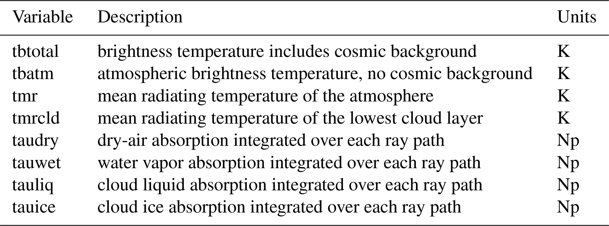
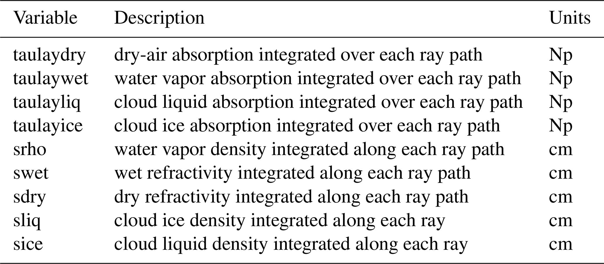
Table 3 List of all the intermediate variables accessible from PyRTlib.

4.1 Simulation of downwelling T_B

As a first example, we propose the simulation of downwelling T_B spectra in a typical MW spectral range. This simple example may become useful in simulating the measurements from a multi-channel ground-based microwave radiometer, e.g., those widely deployed in atmospheric-profiling observatories (Rüfenacht et al., 2021; Shrestha et al., 2022). As input, the user can opt for one of the six climatological atmospheric profiles predefined in PyRTlib (TROPICAL, MIDLAT WINTER, MIDLAT SUMMER, ARCTIC WINTER, ARCTIC SUMMER, US STANDARD; Anderson et al., 1986) or any of the radiosonde/reanalysis profiles retrieved from the repositories introduced in Sect. 3. Listing 4 shows the code to compute and plot downwelling T_B spectra at a frequency resolution of 1 GHz for two typical climatology conditions (tropical and subarctic winter), each at two pointing angles (90 and 30° elevation angle). The graphic output, reported in Fig. 4, shows the typical peaks corresponding to a resonant absorption of atmospheric gases (O₂ at 50–70 and 118 GHz, H₂O at 22.2 and 183 GHz) as well as the non-resonant continuum absorption due to H₂O (monotonically increasing with frequency). The peaks and the continuum show the emission added by the atmospheric gases with respect to the relatively cold emission coming from the outer boundary of the atmosphere (the so-called cosmic background). T_B spectra are generally higher for tropical conditions, due to higher atmospheric temperature and humidity with respect to subarctic winter, and for lower elevation angles, due to the slant longer path traveled by radiation throughout the atmosphere.

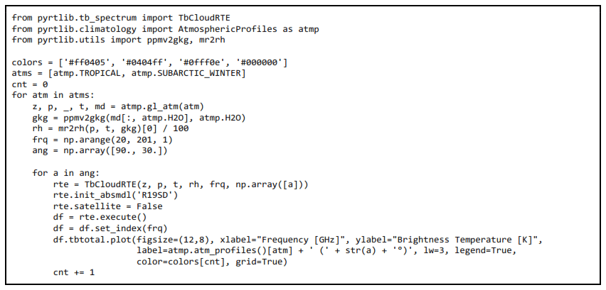
Listing 4 Example code using the PyRTlib module to calculate downwelling T_B in the 20 to 200 GHz spectral range (1 GHz resolution) using two predefined climatological profiles (tropical and subarctic winter) at 90 and 30° elevation angles.

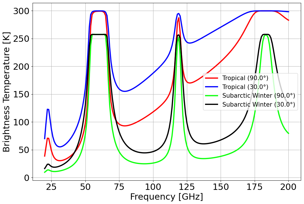
Figure 4 Graphical output of Listing 4, showing downwelling T_B spectra computed for two typical climatologies (tropical and subarctic winter) at two elevation angles (90 and 30°).

4.2 Simulation of upwelling T_B

The second example shows the simulation of upwelling T_B spectra, as those typically sampled by satellite-based MW radiometers (e.g., Moradi et al., 2015). Listing 5 shows the code to compute and plot upwelling T_B spectra at a frequency resolution of 1 GHz for typical midlatitude summer climatology conditions. The graphic output is reported in Fig. 5, where the impact of the pointing angle and surface emissivity is shown by varying their values. In particular, a 90° pointing angle indicates nadir observations, while one at 37° indicates a typical observing angle of MW imagers (53° from nadir), while 0.9 and 0.45 represent typical high and low emissivity values in the MW spectral region. Figure 5 shows that if the emissivity is relatively high (e.g., 0.9), the spectrum resembles that of a warm blackbody emission at ∼270 K (except where strong atmospheric absorption occurs, e.g., 60, 118, and 183 GHz). Conversely, if the emissivity is relatively low (e.g., 0.45), the background is relatively cold and the atmospheric emission features stick out, similarly to Fig. 4. However, near the center of strong emission features (e.g., 60, 118, and 183 GHz) T_B appears flipped with respect to Fig. 4, indicating gas absorption that removes radiation from the emission coming from the relatively warm background. It is notable that in those regions T_B nearly overlaps for the three emissivity and angle conditions; this is because the atmospheric opacity is so high as to make T_B saturate within a short distance, thus becoming insensitive to the surface emission and observing angle (i.e., path length). PyRTlib also allows for frequency-dependent surface emissivity to be provided as input.

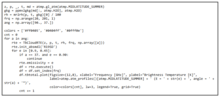
Listing 5 Example code using the PyRTlib module to calculate upwelling T_B in the 20 to 200 GHz spectral range (1 GHz resolution) using a predefined climatological profile (midlatitude summer) at 90 and 37° elevation angles with constant surface emissivity values of 0.9 and 0.45.

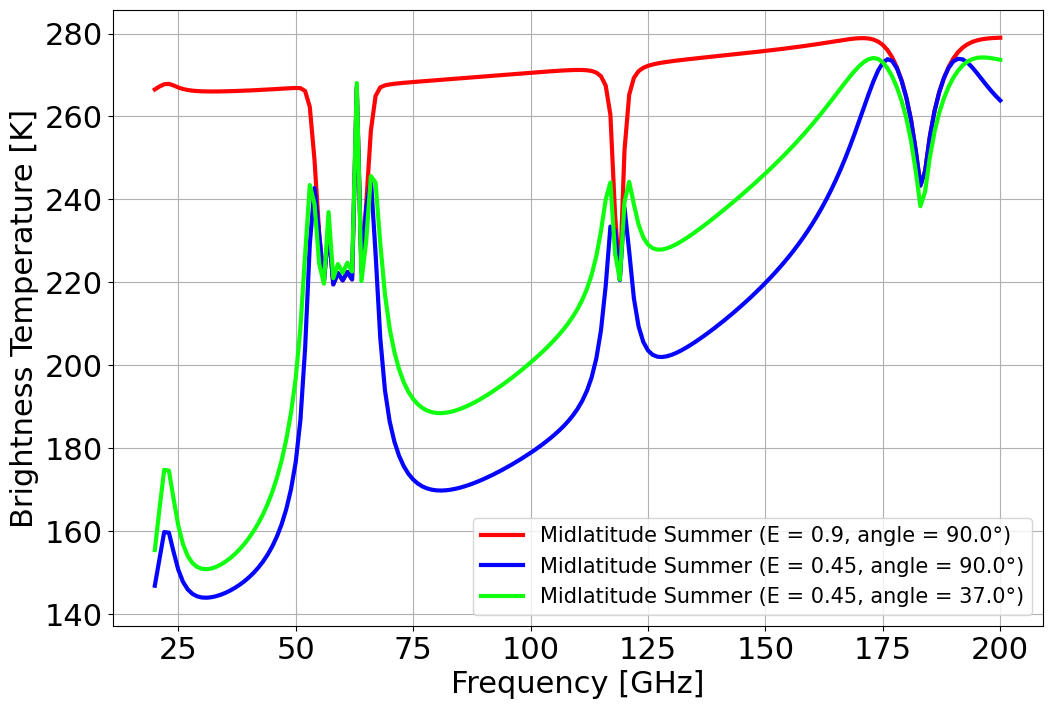
Figure 5 Graphical output of Listing 5, showing upwelling T_B spectra computed for a predefined climatological profile (midlatitude summer) at 90 and 37° elevation angles with constant surface emissivity values of 0.9 and 0.45.

4.3 Simulation of simultaneous downwelling and upwelling T_B

Simultaneous observations of downwelling and upwelling T_B are typically performed from airborne scanning instruments that can alternate between up-looking and down-looking views (e.g., Fox et al., 2017; Wang et al., 2017). Both views can be simulated by PyRTlib using the same atmospheric profile as input and specifying the altitude of the aircraft and the observing angle. Figure 6 shows the downwelling and upwelling T_B simulated assuming the aircraft at 5 km altitude looking down at nadir and up at zenith. The input profile comes from a radiosonde launched from Camborne (UK) at 12:00 UTC on 22 July 2021 and retrieved from the University of Wyoming Upper Air Data archive, corresponding to the location and period of experimental flights by the Facility for Airborne Atmospheric Measurements (FAAM) BAe 146 aircraft mounting the International Submillimetre Airborne Radiometer (ISMAR; Fox et al., 2017). ISMAR has 17 channels spanning the 118 to 874 GHz range, being developed as an airborne demonstrator for the Ice Cloud Imager (ICI), planned for the second generation of European polar-orbiting satellites (Metop-SG; Meteorological Operational satellite) to be launched from 2024. Note that PyRTlib functions allow for displaying and investigating not only T_B but also all the intermediate RT variables, such as absorption, optical depth, and opacity. For example, Fig. 6 shows the atmospheric opacity above and below the aircraft as computed for the up-looking and down-looking views. Atmospheric-absorption spectra from PyRTlib were compared with those computed with ARTS using the equivalent absorption model, resulting in differences within 0.05 %, which are attributed to different assumptions in the variation in the absorption coefficient across an atmospheric layer (Fox et al., 2023).

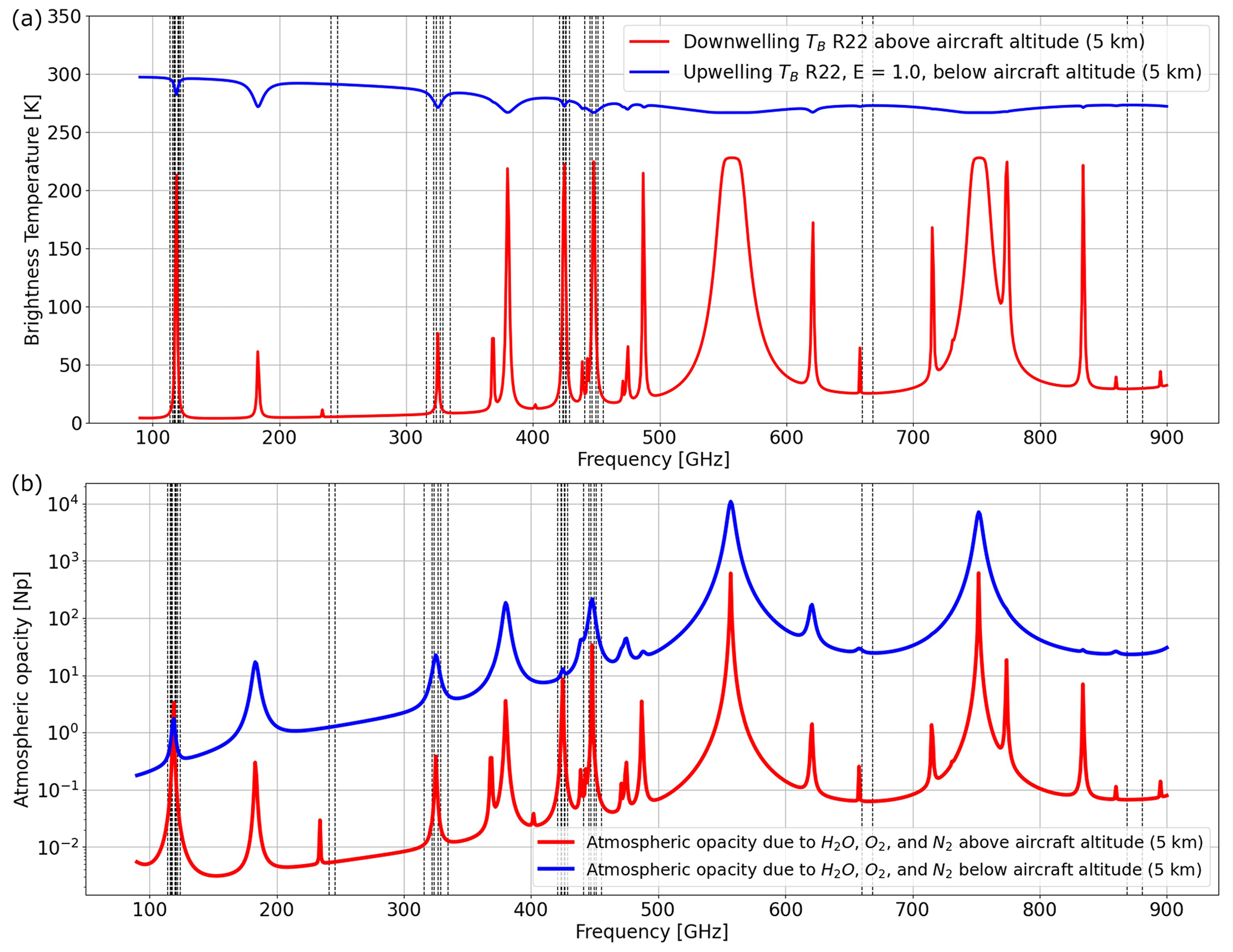
Figure 6 (a) Downwelling and upwelling T_B simulating aircraft observations at zenith and nadir from 5 km altitude, respectively (gas absorption model: R22; surface emissivity equal to 1). (b) Atmospheric opacity (τ) corresponding to dominant gases (H₂O, O₂, and N₂) computed for the up-looking and down-looking views. All the features correspond to H₂O absorption except the following, due to O₂: 118, 368, 424, 487, 715, 773, and 834 GHz. Input profile from the radiosonde launched from Camborne (UK) on 22 July 2021 at 12:00 UTC and retrieved from the University of Wyoming Upper Air Data archive. Vertical black lines indicate the ISMAR channel frequencies.

4.4 Comparison of absorption models

The PyRTlib package allows for T_B simulations with different versions of atmospheric gas absorption models. As mentioned earlier, the spectroscopy underlying absorption models is continuously updated, following the latest findings from laboratory and field campaign experiments. Currently, PyRTlib implements absorption routines originally based on the MPM code (Liebe, 1989) with spectroscopy modified throughout the last decades. Specifically, the following versions are readily callable in PyRTlib (with reference to the paper that motivated the update, where available): R98 (Rosenkranz, 1998), R03 (Tretyakov et al., 2003), R16, R17 (Rosenkranz, 2017), R19, R19SD (Rosenkranz and Cimini, 2019), R20, R20SD (Makarov et al., 2020), R21SD (Koshelev et al., 2021), and R22SD (Koshelev et al., 2022). The original Fortran code for most of these absorption routines by Philip W. Rosenkranz are freely accessible through a repository (http://cetemps.aquila.infn.it/mwrnet/lblmrt_ns.html, last access: 29 February 2024). In the following, we present an example in which the latest version at the time of writing, R22SD, is compared with R98, which still represents a widely used model (e.g., Picard et al., 2009). Modifications in R22SD with respect to R98 include an updated line width at 22 GHz (Payne et al., 2008), updated water vapor continuum coefficients scaled after Turner et al. (2009), revised O₂ mixing coefficients for the 50–70 and 118 GHz lines (Makarov et al., 2020), a speed-dependent line shape for the water vapor absorption lines at 22 (Rosenkranz and Cimini, 2019) and 183 GHz (Koshelev et al., 2021), the addition of four submillimeter-wave water vapor lines (860, 970, 987, 1097 GHz), and other updated line parameters taken from the most recent release of the HITRAN database (HITRAN2020). To test two gas absorption versions, a simple observation-minus-simulation (O-S) approach can be used, exploiting MW ground-based remote sensing and balloon-borne sounding measurements from the US Department of Energy (DOE) Atmospheric Radiation Measurement (ARM) program (https://arm.gov, last access: 29 February 2024), which can be freely accessed from the ARM data center (https://adc.arm.gov, last access: 29 February 2024). In fact, ARM deploys a network of ground-based MW radiometers (MWRs) across its observatory sites (Cadeddu et al., 2013; Cadeddu and Liljegren, 2018). These instruments measure downwelling T_B at selected frequency channels under all-sky conditions. From the same sites, ARM regularly launches radiosondes; the ARM balloon-borne sounding system (BBSS) products provide profiles of in situ measurements of atmospheric pressure, temperature, humidity, and wind speed and direction (Holdridge, 2020), which can be given as input to PyRTlib to simulate zenith downwelling T_B. A dataset of colocated and nearly simultaneous MWR observations and RT simulations can be then used to test and validate simulations from different absorption models. Such a dataset was retrieved from the deployment of the ARM mobile facility in Highland Center, Cape Cod (MA, USA), during the Two-Column Aerosol Project (TCAP) in 2012 (Titos et al., 2014). The observations are the T_B measured by an MWR profiler (MWRP). The MWRP product provides measurements of T_B at 12 frequency channels in the range from 22 to 58 GHz. Frequencies between 22 and 52 GHz are mostly sensitive to atmospheric water vapor and cloud liquid, while frequencies between 51 and 60 GHz are sensitive to atmospheric temperature through the absorption of atmospheric oxygen. Simulations at the same frequency channels are computed from the 4-daily radiosondes (at 05:30, 11:30, 17:30, and 23:30 UTC) launched during TCAP and processed by PyRTlib. To avoid spatiotemporal uncertainty in clouds, the comparison is made in clear-sky conditions, applying a cloud screening to both radiosonde and MWRP data. Clear-sky conditions were selected using a relative humidity threshold, specifically rejecting radiosondes with at least four pressure levels with relative humidity higher than 95 % (Clain et al., 2015). Furthermore, an observation-based screening was applied, removing data for which 1 h standard deviation of the T_B at 30 GHz was larger than 0.5 K, indicating possible obstructions or cloud contamination (De Angelis et al., 2017). From a total of 592 radiosondes, these two screenings leave 149 matchups for the analysis. Simulated and observed datasets were compared by selecting and averaging MWRP observations falling within −45 min to +1 h of each radiosonde launch time, so as to reduce the temporal–spatial mismatch with respect to the radiosonde measurements. The result of the comparison of R98 and R22 models versus the observed dataset is shown in Figs. 7 and 8.

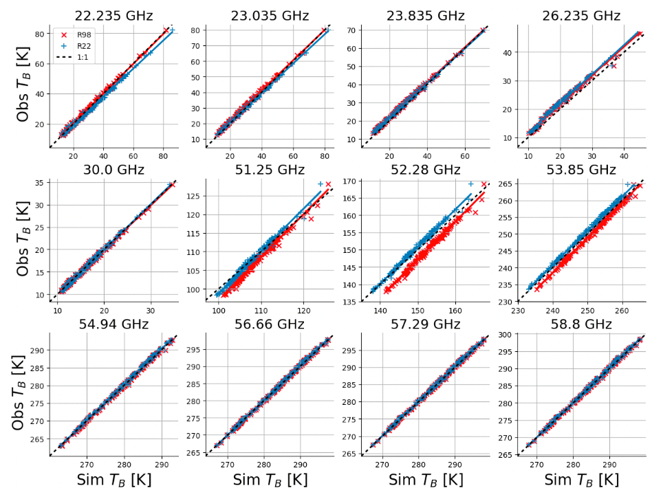
Figure 7 Scatterplots of downwelling T_B as observed by an MWRP (y axis) and simulated with PyRTlib (x axis) using two versions of the gas absorption model (R98 as a red × and R22 as a blue +). Each panel shows one MWRP channel. Markers show 149 MWRP–radiosonde matchups in clear-sky conditions selected from a 6-month period during the TCAP campaign. MWRP and radiosonde data were retrieved from the ARM data center (Cadeddu and Gibler, 2012; Keeler and Burk, 2012).

Figure 7 shows that RT simulations with both absorption models tend to align with observed T_B values over the whole range of variations for all MWRP channels, although larger differences are evident at 51–54 GHz for R98. Bias of the same order of magnitude for the 51–54 GHz channels was previously reported for the R98 model employing MWRs of different types and manufacturers (e.g., Löhnert and Maier, 2012; De Angelis et al., 2017). De Angelis et al. (2017) attribute these to a combination of systematic uncertainties stemming from inaccurate instrument bandpass characterization, instrument calibration, and absorption model. Since then, two major updates have been proposed for the O₂ spectroscopic parameters in this range (mainly mixing coefficients) from laboratory experiments (Tretyakov et al., 2005; Makarov et al., 2020), the latest of which is implemented in R22. Figure 8 reports mean and standard deviation of the simulation-minus-observation differences, which indicate better performances for R22 with respect to R98 in modeling T_B for channels along the low-frequency wing of the O₂ absorption complex, confirming recent independent results (Belikovich et al., 2021, 2022). Unexpectedly, Fig. 8 also indicates differences of ∼2 K for R22 at the 22.2 and 26.235 GHz channels, which will be discussed in next section. PyRTlib also allows for quantifying the impact on T_B of the most recent set of O₂ spectroscopic parameters (Makarov et al., 2020) with respect to the previous one (Tretyakov et al., 2005). In fact, two absorption model versions implemented in PyRTlib, namely R19 and R22, only differ by this aspect in the 50–70 GHz range, and thus the T_B impact is simply evaluated by computing T_B with these two versions and taking the difference. To generalize this, we evaluate the impact by processing the set of 83 diverse atmospheric profiles commonly used to train RTTOV (Saunders et al., 2018). This profile set was carefully chosen from more than 100 million profiles to represent a realistic range of possible diverse atmospheric conditions (Matricardi, 2008), and it is openly available through the Numerical Weather Prediction Satellite Application Facility (NWP SAF) (https://nwp-saf.eumetsat.int/site/software/atmospheric-profile-data/, last access: 29 February 2024). Figure 9 shows the differences between the two models for the downwelling and upwelling T_B simulated at 50 MHz resolution from the 83 diverse profiles, together with the mean difference and standard deviation (SD). For downwelling T_B, the updated O₂ mixing coefficients proposed by Makarov et al. (2020) decrease T_B with respect to the previous ones (Tretyakov et al., 2005) by up to 4–5 K on average, peaking at 53 and 66 GHz, with an estimated global variability of ∼1 K (1σ). For upwelling T_B, the situation is opposite, with a decrease of up to −0.6 K with a 0.2 K SD, although it depends on the assumed surface emissivity (set to 1 in this example).

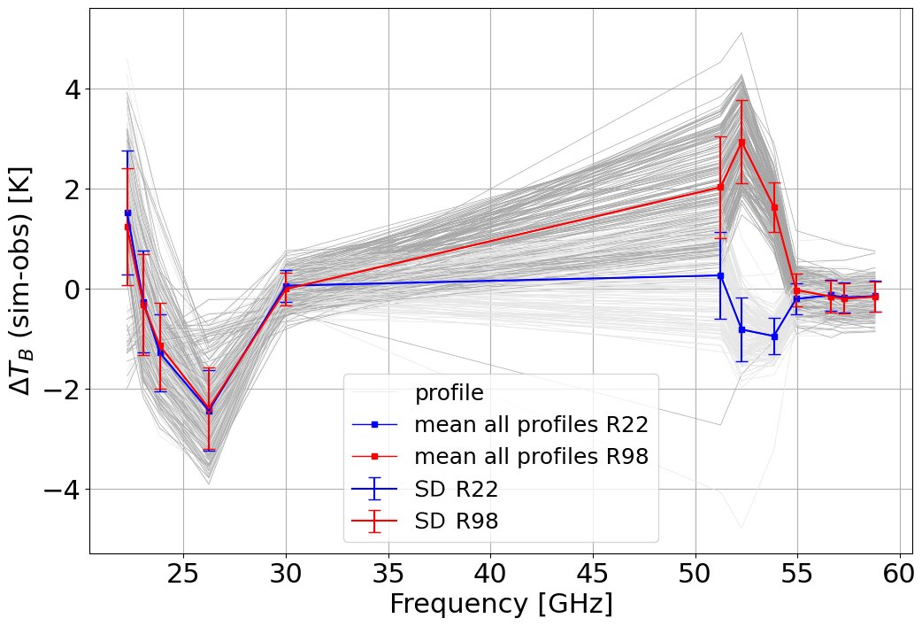
Figure 8 Spectrum of simulation-minus-observation statistics from the 149 MWRP–radiosonde matchups in the clear-sky dataset in Fig. 7. Simulations computed using R98 are shown in red, while those computed using R22 are in blue. Dots and bars indicate the mean value and the standard deviation over the whole dataset, respectively.

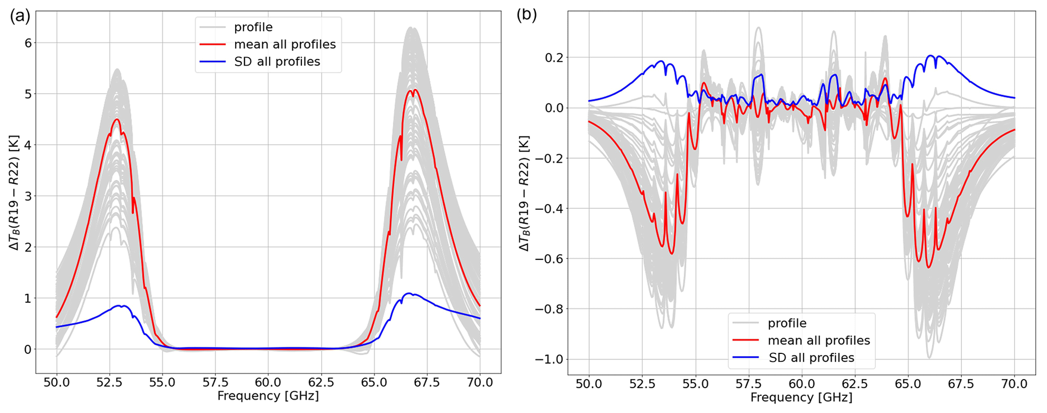
Figure 9 Differences in (a) downwelling and (b) upwelling T_B computed with R19 and R22 absorption models at 50 MHz resolution for the set of 83 diverse NWP SAF profiles. Red and blue lines indicate the mean difference and standard deviation of the dataset. Upwelling simulations assume constant surface emissivity equal to 1.

4.5 Absorption model uncertainty

RT calculations depend on absorption models and the underlying spectroscopic parameters. The values of these parameters are determined through theoretical assumptions or analysis of laboratory or field data and thus are inherently affected by uncertainty. The uncertainty affecting the spectroscopic parameters contributes to the uncertainty in the absorption, which affects the RT calculations and in turn the retrieval of atmospheric variables from remotely sensed observations (Cimini et al., 2018). PyRTlib allows for computing the sensitivity of RT calculations to the uncertainty in various spectroscopic parameters, defined as the T_B difference (ΔT_B) obtained by perturbing the value of the spectroscopic parameter by its uncertainty. Figure 10 reports the sensitivity of zenith downwelling T_B to two water vapor absorption spectroscopic parameters, namely the line intensity (S) at 22.2 GHz and the foreign continuum coefficient (C_f), showing similar results as in the original study (Fig. 2 of Cimini et al., 2018). In addition to the uncertainty in individual parameters, the correlation between the uncertainty in various parameters must also be taken into account, and therefore it is necessary to calculate the complete uncertainty covariance matrix (Rosenkranz, 2005). A general and rigorous approach to estimating the uncertainty covariance matrix for MW absorption models has been outlined (Rosenkranz et al., 2018) and applied to the simulations of downwelling (Cimini et al., 2018) and upwelling (Gallucci et al., 2024) radiation. The full uncertainty covariance matrix from Cimini et al. (2018) is accessible through the PyRTlib code, as well as the Supplement of the original paper (https://acp.copernicus.org/articles/18/15231/2018/acp-18-15231-2018-supplement.zip, last access: 29 February 2024). PyRTlib inherits this development and provides tools to compute T_B together with the associated uncertainty estimate. One example is shown in Fig. 11. It shows ground-based zenith radiometric measurements from the MWRP with its typical calibration uncertainty (Cadeddu and Liljegren, 2018) compared with zenith downwelling T_B computed by processing one radiosonde from the TCAP dataset, together with the associated uncertainty estimate σ(T_B). σ(T_B) is computed within PyRTlib by propagating the spectroscopic parameter uncertainty through the radiative transfer. Calling Cov(p) the parameter uncertainty covariance matrix (as in Cimini et al., 2018) and K_p the sensitivity of T_B to spectroscopic parameter (Jacobian), σ(T_B) is computed as

$${\mathit{\sigma }}^{\mathrm{2}}\left(T_{\mathrm{B}}\right)=\mathrm{diag}\left(\mathbf{Cov}\left(T_{\mathrm{B}}\right)\right)=\mathrm{diag}({\mathbf{K}}_{\mathrm{p}}\cdot \mathbf{Cov}(\mathit{p})\cdot {\mathbf{K}}_{\mathrm{p}}^{\mathrm{T}}),$$

where ^T indicates the matrix transpose. PyRTlib computes the Jacobians K_p by the brute-force method and provides the full covariance matrix of T_B uncertainty Cov(T_B) as output. Figure 11 reports the square root of the diagonal terms (i.e., σ(T_B)), showing that for this single case the observation-minus-simulation differences fit within the overlap of instrumental calibration uncertainty and absorption model uncertainty at the 3σ level and for some channels at the 1σ level. The only channel that is nearly off is 26.235 GHz. This also happens for other radiosondes and absorption models, as is evident in Fig. 8, suggesting that the calibration of this particular channel is questionable and may need a recalibration service.

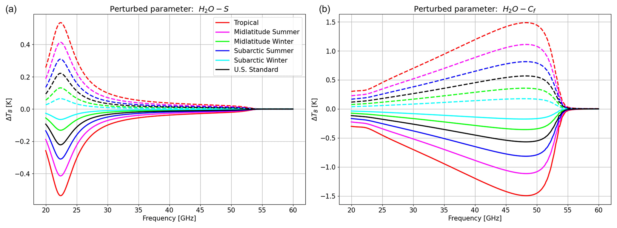
Figure 10 Sensitivity of zenith downwelling T_B to water vapor absorption parameters, computed at 0.1 GHz spectral resolution. (a) Line intensity (S) at 22 GHz. (b) Foreign continuum coefficient (C_f). Solid lines correspond to negative perturbation (value − uncertainty), while dashed lines correspond to positive perturbation (value + uncertainty). Different colors indicate six typical climatological conditions. Adapted from Cimini et al. (2018).

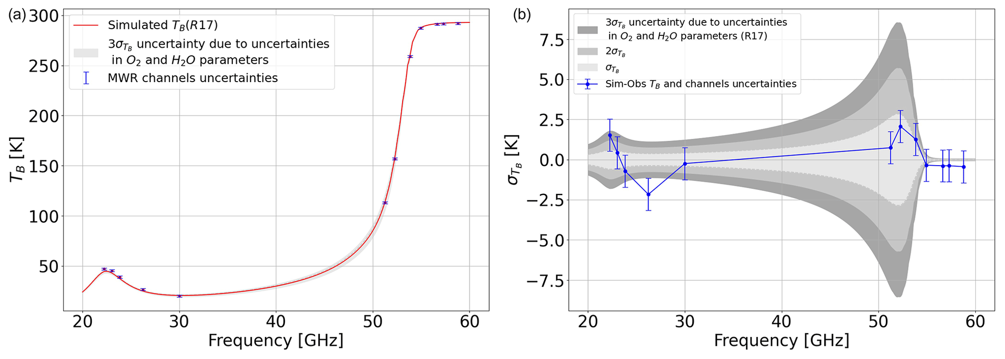
Figure 11 (a) Zenith downwelling T_B spectrum (red line) computed from one radiosonde launched from the ARM mobile facility during TCAP in Cape Cod, MA, USA (26 August 2012, 16:58 UTC). Blue points and bars indicate the nearly simultaneous measurements from the colocated MWRP at 12 frequency channels and their calibration uncertainty. (b) Simulations minus observations at the 12 channels (blue points) with the instrumental calibration uncertainty (blue bars), together with the estimated uncertainty for zenith downwelling T_B (σ(T_B)) due to the uncertainty in absorption model spectroscopic parameters (at 1σ, 2σ, and 3σ levels).

4.6 Radiative forcing versus water vapor concentration

The last example presents an interesting feature of the radiative forcing (i.e., radiance change at the top of the atmosphere) caused by greenhouse gases. It has been demonstrated that such a radiative forcing has a logarithmic dependency on the concentration of some greenhouse gases (e.g., CO₂ and H₂O), and thus the logarithmic scaling of, e.g., CO₂ radiative forcing is often used (IPCC, 2021). This feature is partially attributed to spectrally averaged absorption that saturates logarithmically with the absorber amount (Huang and Bani Shahabadi, 2014), but it was found to also be valid for infrared monochromatic radiance calculations (Bani Shahabadi and Huang, 2014). To explain that, Huang and Bani Shahabadi (2014) proposed the emission layer displacement (ELD) model, based on the vertical displacement of the most contributing layers, which effectively resolves the radiance change as proportional to the logarithm of the gas concentration. However, assumptions underlying the ELD model do not hold for low-opacity frequencies (e.g., window region). In particular, Bani Shahabadi and Huang (2014) indicate that the logarithmic scaling is valid for relatively opaque frequencies (optical depth of >1), while linear scaling is more appropriate for relatively transparent frequencies (optical depth of ≤1). To our knowledge, this has not been verified at microwave frequencies yet, though it can be easily tested with PyRTlib as follows. Considering the standard tropical atmosphere and nadir viewing, brightness temperatures are computed at two frequencies corresponding to relatively weak and strong H₂O absorption lines (i.e., 22.235 and 183.0 GHz). For each frequency, T_B values are computed seven times by multiplying the water vapor mixing ratio by the following scaling factors (SF${}_{q_{{\mathrm{H}}_{\mathrm{2}}\mathrm{O}}}$): $\mathrm{1}/\mathrm{8}$, $\mathrm{1}/\mathrm{4}$, $\mathrm{1}/\mathrm{2}$, 1, 2, 4, and 8. Figure 12 shows the brightness temperatures difference (ΔT_B) with respect to the unperturbed tropical profile plotted against the binary logarithm of the scaling factor. The logarithmic relationship between ΔT_B and water vapor concentration is evident for high atmospheric absorption at 183 GHz (opacity of ∼6 to 262). Conversely, for the relative weak absorption at 22.2 GHz, the relationship changes from linear to logarithmic as the opacity increases from 0.05 to 1.86, showing a dip at ∼1 Np.

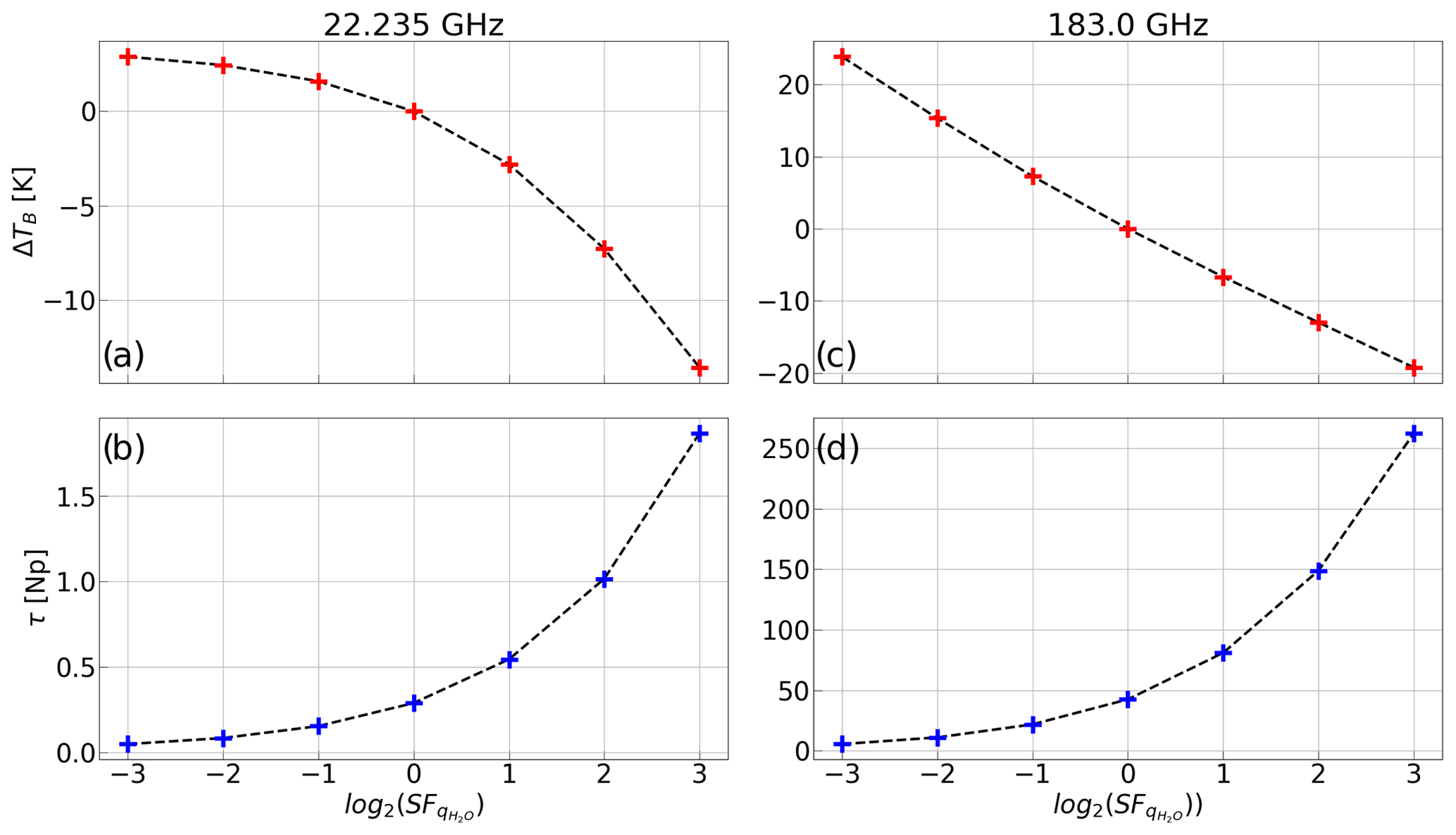
Figure 12 (b, d) Atmospheric opacity τ at (b) 22.235 and (d) 183.0 GHz versus log₂ of the water vapor concentration scaling factor (SF${}_{q_{{\mathrm{H}}_{\mathrm{2}}\mathrm{O}}})$. (a, b) Corresponding change in zenith upwelling monochromatic T_B (ΔT_B) for relatively (a) low opacity at 22.235 GHz and (c) high opacity at 183.0 GHz.

5 Summary and future developments

This paper presents PyRTlib version 1.0, a Python library for non-scattering atmospheric microwave radiative transfer computations. The intention for PyRTlib is to provide a user-friendly tool for computing down- and upwelling brightness temperatures and related quantities (e.g., atmospheric absorption, optical depth, opacity) in Python, a flexible language that is nowadays the most used one for scientific software development, especially by students and early-career scientists. Within its limits, mainly non-scattering and 1-D geometry, PyRTlib allows for simulating observations from ground-based, airborne, and satellite microwave sensors in clear-sky and in cloudy conditions (under Rayleigh approximation). Clearly, the intention for PyRTlib is not to be a competitor to other radiative transfer codes that excel in computational efficiency (RTTOV, CRTM), flexibility (ARTS), modularity (ARTS, Py4CAtS), and applicability (ARTS, PAMTRA). Nevertheless, despite the speed limitations and the omission of important aspects of RT (e.g., spherical geometry and particle scattering), we believe PyRTlib is attractive as an educational tool because of its flexibility and ease of use, providing a quick interface to popular repositories of atmospheric profiles from radiosondes and model reanalysis. PyRTlib also allows for specific investigations such as absorption model comparison and validation against observations (e.g., Sect. 4.4) and the estimation of brightness temperature uncertainty due to an atmospheric-absorption model (e.g., Sect. 4.5). In addition, PyRTlib could be used as a module for other Python codes that need atmospheric radiative transfer, e.g., the Snow Microwave Radiative Transfer model (SMRT; Picard et al., 2018). Future developments include the implementation of (i) new absorption models (e.g., R23 came out at the time of submission); (ii) sensor-oriented calculations considering channels' spectral response functions; (iii) uncertainty estimates for higher-frequency brightness temperature calculations, as was recently investigated (Gallucci et al., 2024); (iv) additional tools for extrapolating the input profiles (e.g., Annex 3 of ITU-R P.835-6, 2017); (v) calculation of weighting functions; and (vi) additional tools for accessing other open atmospheric-data repositories to be used as RT calculation input, e.g., the ARM data center and the Global Climate Observing System Reference Upper-Air Network (GRUAN; Bodeker et al., 2016).