the Creative Commons Attribution 4.0 License.
the Creative Commons Attribution 4.0 License.
 | 28 Feb 2024
MQGeometry-1.0: a multi-layer quasi-geostrophic solver on non-rectangular geometries
Louis Thiry
Guillaume Roullet
Etienne Mémin
This paper presents MQGeometry, a multi-layer quasi-geostrophic (QG) equation solver for non-rectangular geometries. We advect the potential vorticity (PV) with finite volumes to ensure global PV conservation using a staggered discretization of the PV and stream function (SF). Thanks to this staggering, the PV is defined inside the domain, removing the need to define the PV on the domain boundary. We compute PV fluxes with upwind-biased interpolations whose implicit dissipation replaces the usual explicit (hyper-)viscous dissipation. The discretization presented here does not require tuning of any additional parameter, e.g., additional eddy viscosity. We solve the QG elliptic equation with a fast discrete sine transform spectral solver on rectangular geometry. We extend this fast solver to non-rectangular geometries using the capacitance matrix method. Subsequently, we validate our solver on a vortex-shear instability test case in a circular domain, on a vortex–wall interaction test case, and on an idealized wind-driven double-gyre configuration in an octagonal domain at an eddy-permitting resolution. Finally, we release a concise, efficient, and auto-differentiable PyTorch implementation of our method to facilitate future developments on this new discretization, e.g., machine-learning parameterization or data-assimilation techniques.
- Article
(3980 KB) - Full-text XML
- BibTeX
- EndNote


Ocean fluid dynamics offers a hierarchy of models with a trade-off between the richness of the physical phenomena and the dimensionality of the system. On the one end of this hierarchy are the Boussinesq non-hydrostatic equations. These equations describe the evolution of the stratification via temperature and salinity; they model explicitly convective phenomena but they require the evolution of six prognostic variables: the three components of the velocity ; temperature T and salinity s; and the free surface η.
On the other end of this hierarchy are the multi-layer quasi-geostrophic equations. These equations are based on strong hypotheses: static background stratification as well as hydrostatic and geostrophic balances. In a multi-layer quasi-geostrophic (QG) model, the stream function (SF) ψ and potential vorticity (PV) q are stacked in N isopycnal layers with density ρi and reference thickness Hi:
The governing equations read
stands for the horizontal orthogonal gradient, and denotes the horizontal Laplacian. is the Coriolis parameter under beta-plane approximation with the meridional axis center; y0, is the gravitational acceleration; and denotes the reduced gravities. One can include bottom topography as a constant term on the r.h.s. of the QG elliptic Eq. (1b) (Hogg et al., 2014).
QG equations hence involve a single prognostic variable, the potential vorticity (PV) q, which is advected (Eq. 1a). Despite strong hypotheses, the multi-layer QG equations are a robust approximation of ocean meso-scale non-linear dynamics. They offer a computationally efficient playground to study the meso-scale ocean dynamics and to develop physical parameterizations of the unresolved eddy dynamics (e.g., Marshall et al., 2012; Fox-Kemper et al., 2014; Zanna et al., 2017; Ryzhov et al., 2020; Uchida et al., 2022).
Solving the QG equations requires solving an elliptic equation (Eq. 1b) which relates the SF ψ and the potential vorticity q. On a rectangular domain, it can be easily achieved using a fast spectral solver based on discrete Fourier transform (DFT) for periodic boundary conditions or discrete sine transform (DST) for no-flow boundary conditions. Most of the available open-source QG solvers such as GeophysicalFlows (Constantinou et al., 2021), PyQG, or Q-GCM (Hogg et al., 2014) use such spectral solvers and are therefore limited to rectangular geometries.
There are two major issues when implementing QG models on non-rectangular geometries. The first issue is the fact that spectral elliptic solvers do not apply to non-rectangular domains. In ocean models, one typically uses conjugate gradient (CG) iterative solvers such as BiCGSTAB (Van der Vorst, 1992) to solve elliptic equations on non-rectangular domains, for example, when solving the Poisson equations associated with a rigid-lid constraint (Häfner et al., 2021) or for implicit free-surface computations (Kevlahan and Lemarié, 2022) in primitive equation solvers. These CG iterative solvers are significantly slower than spectral solvers for solving Poisson or Helmholtz equations on evenly spaced rectangular grids (Brown, 2020). Using them in a QG solver would reduce significantly the computational efficiency that makes QG appealing compared to shallow-water (SW) models.
The second issue is the definition of the potential vorticity (PV) on the boundaries. If we discretize the PV q on the same locations as the SF ψ, we have to define the PV on the boundaries. This requires using a partial free-slip/no-slip condition (see, e.g., Hogg et al., 2014) to define ghost points in order to compute the Laplacian of the SF.
In this paper, we present MQGeometry, a new multi-layer QG equation solver that addresses these two issues. This solver uses a new discretization of the multi-layer QG equations based on two main choices. The first choice is to discretize the potential vorticity (PV) and the stream function (SF) on two staggered grids. When doing so, the PV is not defined on the boundary of the domain but in its interior. This solves the issue of defining the PV on the domain boundaries. Moreover, this choice makes it possible to use a finite-volume scheme for the PV advection. It guarantees the global conservation of the PV and leverages a fine control on the PV fluxes. The second choice is to solve the elliptic equation using a fast spectral DST solver combined with the capacitance matrix method (Proskurowski and Widlund, 1976) to handle non-rectangular geometries.
In addition to these two choices, we decide to compute PV fluxes with upwind-biased stencil interpolation to remove the additional (hyper-)viscosity used in most discrete QG models. Doing so, we explore a different approach that is complementary to physical parameterizations of the horizontal momentum closure: a careful choice of the numerical schemes used to discretize the continuous equations. This idea has been initially developed by Boris et al. (1992) in the context of large eddy simulation (LES) models and made popular as implicit LES by Grinstein et al. (2007). It has been successfully tested by Von Hardenberg et al. (2000) to study vortex merging in a single-layer QG model and by Roullet et al. (2012) to study the forced-dissipated three-dimensional QG turbulence in a channel configuration. While Von Hardenberg et al. (2000) and Roullet et al. (2012) used only linear upwind-biased reconstruction, we implement here linear and non-linear weighted essentially non-oscillatory (WENO) reconstructions (Jiang and Shu, 1996; Borges et al., 2008) that are tailored to remove spurious numerical oscillations created by linear reconstructions (Liu et al., 1994).
We implement the proposed discretizations in a concise Python PyTorch code that enables seamless GPU acceleration. It benefits from built-in automatic differentiation to facilitate future development in machine learning or data assimilation. We validate our solver on a vortex-shear instability test case in a closed squared domain, an inviscid vortex–wall interaction, and an idealized wind-driven double-gyre configuration in a non-rectangular configuration.
This paper is organized as follows. In Sect. 2, we describe the resolution of the PV advection equation with finite volume. In Sect. 3, we present our elliptic solver based on discrete sine transform and the capacitance matrix method (Proskurowski and Widlund, 1976). In Sect. 4, we detail the solver implementation. In Sect. 5, we describe the experimental settings to validate our discretization. We conclude and evoke further perspectives in Sect. 6.
2.1 Staggered discretization of PV and SF
The first ingredient of our method is to use finite volumes to solve PV advection (Eq. 1a). This leads naturally to a staggered discretization for the PV and the SF (see right panel of Fig. 1). With this choice, the PV advection (1a) can be integrated over the whole domain as a transported tracer with a finite-volume formulation. Indeed, if ψ is discretized at the cell vertices, the orthogonal gradient of ψ computed with the standard second-order discretization
lies in the middle of the cell edges. The horizontal velocity u lives in the middle of the vertical edges while the vertical velocity v lives in the middle of the vertical edges. We thus have to discretize the PV q at the cell centers to solve its advection with finite volumes.
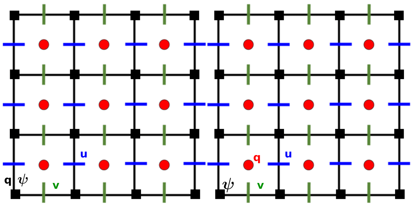
Figure 1Usual (left) and proposed (right) staggered discretization (bottom) of the prognostic variables (q, ψ, u, v) for the QG system (1).
At the boundary which passes along the cell edges, the condition is simply the non-flux of PV across the walls. This staggering clearly separates the boundary condition associated with the transport of PV from the boundary condition associated with optional friction (partial free-slip or no-slip). The global conservation of PV during advection is ensured up to numerical precision with finite volumes.
In the usual discretization (see Appendix A), the PV must be defined on the boundary, which requires definition of the Laplacian operator Δh there. This is problematic since it forces blending of the slip boundary conditions into the definition of the Laplacian, rather than having a slip boundary condition clearly separated from the definition of PV. Moreover, depending on this choice, the material conservation of the PV might not be ensured even though the advection scheme, e.g., Arakawa–Lamb (Arakawa and Lamb, 1981), conserves the PV inside the domain.
2.2 Upwinding of PV fluxes
In a finite-volume formulation, we rewrite the PV advection (1a) as the divergence of a flux:
The divergence is discretized with the usual second-order finite-difference operator
We hence need to interpolate q on the u and v grid points to compute these PV fluxes. In the context of finite-volume methods, we call these interpolations reconstructions.
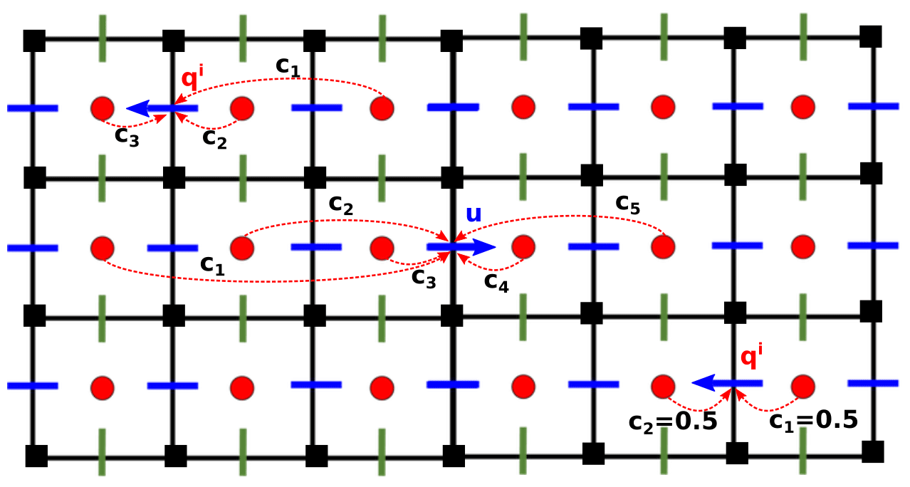
Figure 2Illustration of the upwind-biased reconstruction. Away from boundaries we use a five-point stencil for reconstruction, while close to boundaries, we use a three-point stencil when possible (top-left). At distance 1 from the boundary when the velocity moves away from the boundary (bottom-right), we use a second-order reconstruction with a two-point centered stencil rather than upwind-1 reconstruction to have a reconstruction of the order of 2 at least. For linear reconstructions, the weights ci are fixed. For non-linear reconstruction, the weights ci depend on the solution.
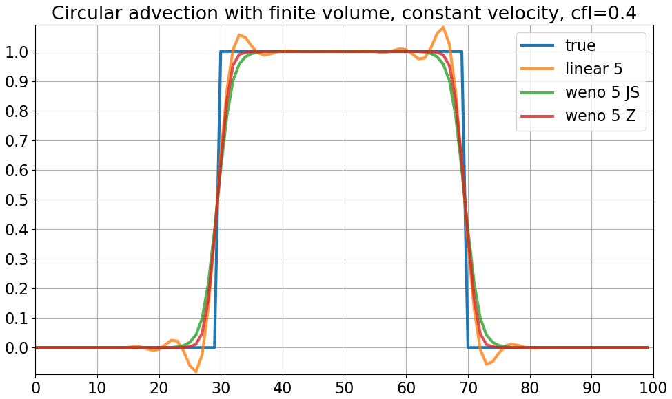
Figure 3One-dimensional advection with constant velocity on a periodic domain over one period. We compare three finite-volume methods using linear, WENO-JS (Jiang and Shu, 1996), and WENO-Z (Borges et al., 2008) five-point upwind reconstructions.
For a good trade-off between stability and accuracy, we use a five-point upwind-biased stencil for reconstruction. Near the boundary we use a three-point upwind-biased stencil or a two-point centered stencil as illustrated in Fig. 2. The ordering of the stencil is given by the sign of the velocity. For instance, when the velocity is positive, and we have the reverse order when the velocity is negative. Using upwind-biased stencils for reconstruction allows us to remove additional ad hoc (hyper-)viscosity, which is necessary when using centered reconstructions (Lemarié et al., 2015). We decide here to rely solely on the upwinding to handle the potential enstrophy dissipation, which is done implicitly.
We offer two possibilities for reconstructions: linear reconstructions or weighted essentially non-oscillatory (WENO) reconstructions (Liu et al., 1994). The weights cs are fixed for the linear reconstruction. However, flux computed with linear reconstructions tends to produce spurious numerical oscillations when the field q is not smooth (see Fig. 3).
WENO reconstructions benefit from the essentially non-oscillatory property (Harten, 1984): they are designed to prevent spurious numerical oscillations that occur with linear reconstructions (see Fig. 3). With a WENO scheme, the weights cs are not fixed: they depend on the value of q on the five-point stencil via smoothness indicators, e.g., first- and second-order derivatives computed with finite difference (Jiang and Shu, 1996). The smoother the q on the stencil, the closer the weights cs are to the linear weights. One can find a detailed explanation of these non-linear weight computations in Borges et al. (2008).
2.3 Time integration
The convergence and stability properties of WENO schemes derived in Jiang and Shu (1996) require the use of a total variation diminishing (TVD) Runge–Kutta scheme of the order of 3 at least (Shu and Osher, 1988). Here we use a TVD Runge–Kutta scheme of the order of 3 (TVD RK3) for time integration with finite time step δt.
Given the time ordinary differential equation
one can write the TVD RK3 scheme with the following three stages:
This low-memory version requires only the storage of the intermediate time derivatives Lf(i).
3.1 Staggering of PV and SF
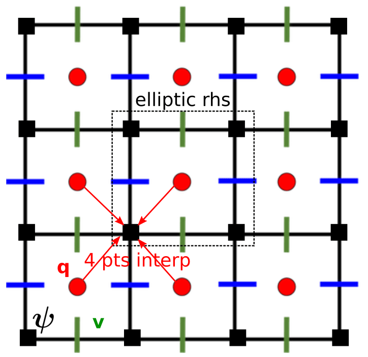
After having solved PV advection equation (Eq. 1a), one has to solve the elliptic Eq. (1b) to compute the SF. The SF ψ satisfies the homogeneous Dirichlet boundary condition; hence we have to compute the r.h.s. terms inside the domain. Due to the staggered discretization, we need to interpolate them between the two grids. A natural way to proceed is to use a four-point linear interpolation to interpolate q on the ψ grid (see Fig. 4).
3.2 DST solver on rectangular geometry
To solve the elliptic Eq. (1b), we use a vertical transform and a fast spectral solver with discrete sine transform (DST). One can diagonalize the matrix A (defined in Eq. 1c) as follows:
where the layer-to-mode matrix Cl2m is the inverse of the mode-to-layer matrix Cm2l, and Λ is a diagonal matrix containing A eigenvalues. One can then perform the following layer-to-mode transform:
With this transform, the elliptic Eq. (1b) becomes a stack of N two-dimensional Helmholtz equations
with homogeneous Dirichlet boundary conditions. To solve these N two-dimensional Helmholtz equations, we use fast diagonalization with type-I discrete sine transform (DST-I) since the usual five-point Laplacian operator
becomes a diagonal operator in the type-I sine basis (Press and Teukolsky, 2007, Chap. 20.4, p. 1055). After having solved these N Helmholtz equations, we transform back ψ from mode to layers:
3.3 Capacitance matrix method for non-rectangular geometry
To handle non-rectangular domains, we use the capacitance matrix method (Proskurowski and Widlund, 1976). We have a non-rectangular domain , where ∂Ω is the domain boundary and is the interior of the domain. Our non-rectangular domain Ω is embedded in a rectangular domain . We denote by the set of non-rectangular boundary indices (see Fig. 5). We assume that we have K non-rectangular boundary points Ik∈ℐ.
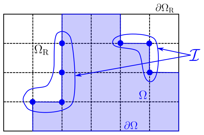
Figure 5Domain Ω included in a rectangular domain ΩR and the set of non-rectangular boundary indices.
We now explain how to solve the following non-rectangular Helmholtz equation:
One can find a more detailed explanation in Blayo and LeProvost (1993), as this is our inspiration for using the capacitance matrix method.
3.3.1 Precomputations
For each non-rectangular boundary point Ik∈ℐ, a Green function gk is defined as the solution of the following rectangular Helmholtz equation:
solved using DST-I fast diagonalization. With these Green functions, we compute the square matrix M with coefficients
We compute this matrix inverse to get the so-called capacitance matrix .
3.3.2 First step
In the first step, we solve the following rectangular Helmholtz equation:
using DST-I fast diagonalization. We then compute the vector s coefficients
and we deduce the vector
3.3.3 Second step
In the second step, we solve the following rectangular Helmholtz equation:
using DST-I fast diagonalization. This function f(2) is such that
The restriction of f(2) over our non-rectangular domain Ω is therefore the solution of the Helmholtz Eq. (4).
3.3.4 Numerical cost
The capacitance matrix method involves solving a dense linear problem with K unknowns, K being the number of boundary irregular points ℐ. The capacitance matrix is hence a K×K matrix, and its inversions require 𝒪(K3) computations.
In practice, the inversion is the most computationally expensive operation, but it is precomputed a single time. The major limitation of this method is in terms of memory, i.e., to store the K×K matrix especially on GPUs whose memory capacity is usually smaller than CPUs. On the laptop utilized, we were able to use up to K=10 000, allowing us to run simulations akin to the North Atlantic at a resolution of 6 km. At this resolution, the ageostrophic effects become significant, and the QG hypothesis might no longer be relevant.
4.1 Programming language and library
One can implement the above discretization using any programming language. To anticipate later applications in data assimilation and machine learning, and to benefit easily from GPU acceleration, we have decided to use the PyTorch library (Paszke et al., 2019). This library contains the usual linear algebra routines, and the computations can be easily vectorized. It offers a built-in automatic differentiation to compute gradients or adjoints. This can be beneficial for future machine-learning and data-assimilation developments.
4.2 Upwind flux computation
Upwind flux computations require splitting the velocity into a positive and a negative part. This can be achieved very efficiently using the ReLU function
whose PyTorch implementation is highly optimized since this function is widely use in neural networks. The positive part u+ and negative part u− of the velocity are given by
4.3 WENO reconstructions
Weighted essentially non-oscillatory (WENO; Liu et al., 1994) is a large class of reconstruction methods. We implement two of the most widely used WENO reconstructions: WENO-JS (Jiang and Shu, 1996) and WENO-Z (Borges et al., 2008). Implementing these methods requires only a few lines of Python code (shown in Listing B1 in Appendix B).
4.4 Masks
For the non-rectangular domain, one has to provide a binary mask for the PV grid with ones inside the domain and zeros outside. Given this mask, we automatically compute the masks for the other variable, i.e., the SF ψ and the two components of the velocity u and v, and we deduce the non-rectangular boundary set ℐ involved in the capacitance matrix computations. We also compute specific masks that specify the stencil for PV reconstruction on u and v points for PV fluxes computations. This is illustrated in Fig. 6.
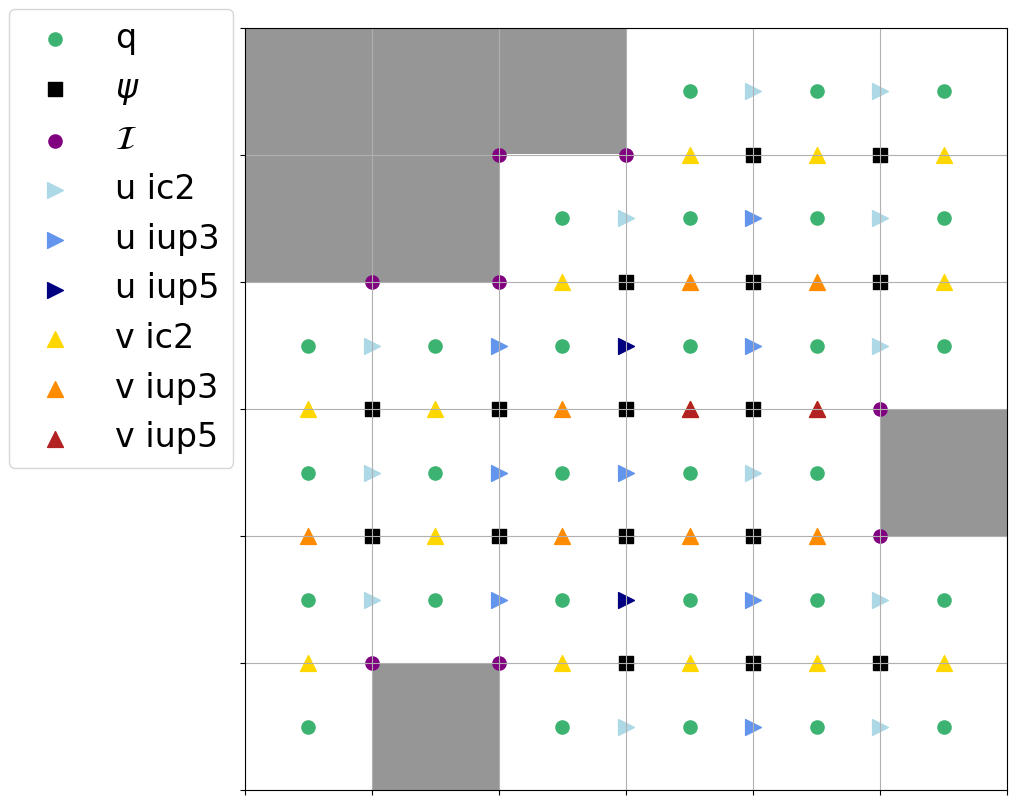
Figure 6Illustration of the different masks. The label “u ic2” means that one uses two-point centered stencils to reconstruct q on these u points for computations of PV fluxes. The label “v iup5” means that one uses five-point upwind-biased stencils to reconstruct q on these v points for computations of vertical PV fluxes.
4.5 Elliptic solver
Our elliptic solver is based on fast diagonalization using discrete sine transform. Since PyTorch implements FFT but not DST, we implement DST-I using FFTs with specific pre- and post-processing operations. Notably, our DST-I implementation is faster than SciPy's implementation on Intel CPUs thanks to PyTorch bindings to MKL FFT.
The capacitance matrix method implementation is straightforward following the equations in Sect. 3. Capacitance matrices are precomputed given the set of non-rectangular boundary indices ℐ. The method solves the Helmholtz equation with machine precision accuracy. Figure 7 illustrates this point on a circular domain at resolution 2562. From a prescribed stream function f, taken as Gaussian white noise and vanishing along the boundary, we apply the Helmholtz operator to get a r.h.s. We then solve the Helmholtz equation with this r.h.s. to get finv. Figure 7 shows that finv−f is of the order of machine precision. The method is independent of the domain shape. The numerical experiments below explore various domain shapes.
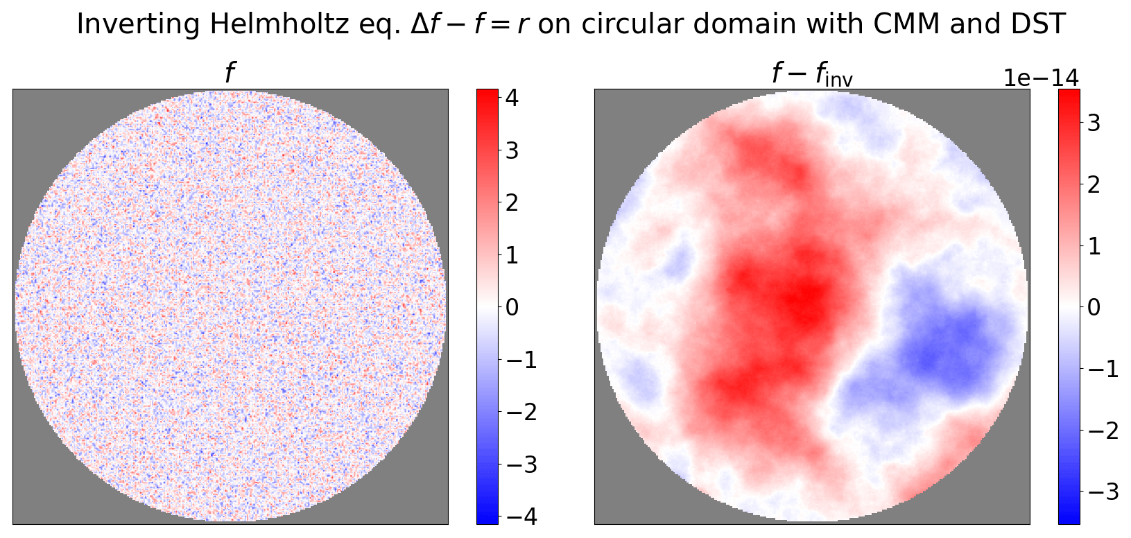
Figure 7Example of Helmholtz equation solved with our solver on a circular domain embedded in a 2562 square domain. The true function f is initialized with spatially uncorrelated Gaussian white noise. The inverted function finv is computed using our solver. The difference between f and finv is of the order of machine precision. CMM stands for capacitance matrix method.
Our spectral solver cannot handle curvilinear coordinates or non-constant metric terms. Solving the QG equations on a grid with non-constant metric terms requires an iterative elliptic solver, e.g., a multigrid solver (Fulton et al., 1986). Iterative solvers can be sped up with a good initial guess. One can still use the solver presented here to provide an initial guess assuming that the metric terms dx and dy are constant, e.g., equal to the mean dx and dy.
4.6 Compilation
PyTorch embeds a compiler which enables a significant speed-up for computationally intense routines. We compile the flux computations and finite-difference routines. We get a 2.2× speed-up thanks to this compilation with torch.compile.
4.7 Ensemble simulations
Thanks to PyTorch vectorized operations, our implementation allows us to run ensemble simulations, i.e., parallel simulations starting from different initial conditions. This is a promising possibility for later developments of ensemble-based data assimilation or for stochastic extensions such as Li et al. (2023).
4.8 Architecture
The code is divided into six Python scripts:
-
helmholtz.py, which contains the Helmholtz solvers based on DST-I and the capacitance matrix method -
fd.py, which contains the finite-difference functions -
reconstruction.py, which contains the reconstruction (i.e., interpolations in the context of finite volumes) routines -
masks.py, which contains the mask utility module -
flux.py, which contains the flux computation routines -
qgm.py, which contains the Python class implementing the multi-layer QG model.
We end up with a concise PyTorch implementation (∼ 750 lines of code) which is as close as possible to the equations. It can run seamlessly on CPUs and GPUs with CUDA compatibility.
4.9 Performance
To assess the performance of our solver, we ran the double-gyre experiment (see below) on a Dell Precision 7560 laptop equipped with an Intel Core i9-11950H CPU and an NVIDIA RTX A3000 laptop GPU. We measure the number of seconds per grid point per time step as well as the power consumption of the devices using the commands nvidia-smi for GPU and turbostat for CPU.
Using the GPU, we get an execution time of s per grid point per time step with a power consumption of 75 W. Using the CPU with a single core, we get an execution time of s per grid point per time step with a power consumption of 22 W. Using the full CPU with 16 cores, we get an execution time of s per grid point per time step with a power consumption of 67 W.
As expected, the GPU has a better power efficiency than the CPU (Häfner et al., 2021). There is still room for improvement for CPU parallelization in our code, as the native parallelism of PyTorch is not fully efficient in our case.
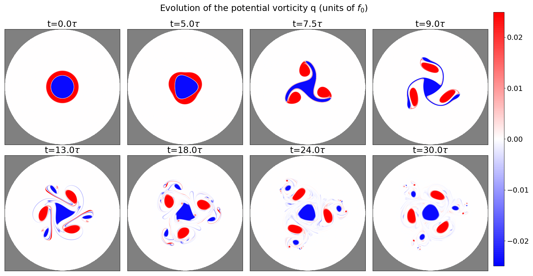
Figure 8Vortex-shear instability experiment. Evolution of potential vorticity q at initial time t=0; at intermediate times , and 24τ; and at final simulation time 30τ.
4.10 Accuracy
Despite the high-order WENO reconstruction used to solve the PV transport, our solver is formally second-order accurate due to the staggering and the use of a second-order perpendicular and divergence operator. This calls for a discussion.
The perpendicular gradient operator is applied to the SF, which is the smoothest field that we resolve. The benefits of using higher-order schemes for this operator are less obvious. The second-order divergence operator used in finite-volume advection ensures the global conservation of PV up to numerical precision. Higher-order schemes might discard this conservation property. For the PV advection, low-order reconstruction schemes suffer from higher numerical diffusion (Lemarié et al., 2015) while linear reconstructions tend to create more oscillations for non-smooth fields. These two considerations motivate the use of high-order non-linear reconstruction on the PV field, which is non-smooth since QG flows contain boundary currents, eddies, and filaments.
We run three numerical experiments involving meso-scale vortices (20–200 km diameters) to validate our solver. The first one is a vortex-shear instability, the second is a vortex–wall interaction, and the third is an idealized double-gyre experiment, which is a usual toy model for western boundary currents. With our solver, multi-layer QG equations deliver on their promise of a computationally efficient playground to study meso-scale non-linear dynamics. Indeed, the three experiments presented here ran on a laptop and took a few to 50 min to run. We provide the Python scripts to reproduce these experiments and the figures.
5.1 Vortex-shear instability
The first validation of our method consists of a vortex-shear instability. We consider a rotating fluid in a circular domain with diameter D=100 km embedded in a square domain of size 100 km× 100 km on an f plane with a Coriolis parameter f0, whose value is deduced from the Burger number below. There is a single layer of fluid with reference thickness H=1 km. We assume no-flow and free-slip boundary conditions. The gravity constant is set to g=10 m s−2.
We study the shear instability of a meso-scale shielded Rankine vortex, which has piece-wise constant PV. In the initial state, the vortex is composed of a core vortex surrounded by a ring of opposite-sign PV to the core such that the total sum of the PV is 0. This system is shear unstable and generates multipoles (Morel and Carton, 1994). We focus here on the tripole formation regime.
The core of the vortex has a radius r0=10 km and positive vorticity. The surrounding ring has an inner radius r0=10 km and r1=14 km. The remaining parameters of the simulation are set via the Rossby and Burger numbers defined as follows:
where umax is the maximum velocity of the initial condition. Given the Burger number, we compute the Coriolis parameter using . Then given the Rossby number, we rescale the velocity field of the initial condition such that the maximum velocity is umax=Rof0r0. The quasi-geostrophic equations are valid for Bu≤1 and Ro≪1. We perform the experiment with Ro=0.01 and Bu=1. The equations are integrated over a period of 30 τ, with the eddy-turnover time and qinit the initial condition, shown at the top left of Fig. 8. At initial time the PV contours of the core and the ring r=ri are slightly perturbed by means of a mode-3 azimuthal perturbation defined in polar coordinates (r,θ) by
where ϵ≪1 is a small parameter, typically ϵ=0.001. This perturbation favors the growth of the most unstable mode which, given the ratio , evolves non-linearly into a tripole (Morel and Carton, 1994).
We use WENO-Z reconstructions for this experiment. This experiment can be reproduced with script vortex_shear.py. We run the reference experiment at a resolution of 10242.
We see in Fig. 8 the evolution of the vortex PV q at different times between the beginning and the end of the simulation at time t=30 τ. At time t=5 τ the result of the instability is visible and the core vortex which was initially circular has a triangular shape. At time t=7.5 τ the outer positive PV ring has become the expected tripole (Morel and Carton, 1994). At time t=9 τ the core vortex recovers a triangular shape with negative PV filaments ranging from the triangle vertices to the three positive vortices. At time t=13 τ, the core vortex keeps a triangular shape and the vorticity filaments become thinner. At time t=18 τ, the filament thickness reaches the grid scale and the filaments start being dissipated by WENO-Z implicit dissipation. At time t=24 τ, the filaments are progressively dissipated and have a smaller amplitude. The core vortex shape becomes more circular, and the three positive vortices are surrounded by a smaller negative vortex. At final time t=30 τ, the filament amplitude has lowered, and small vorticity dipoles appear. The order-3 symmetry, which was injected by the initial perturbation, starts to be lost only at time t=30 τ. For later times (not shown), the system evolves into a chaotic system. This chaotic evolution is expected as the system is sensitive to initial conditions.
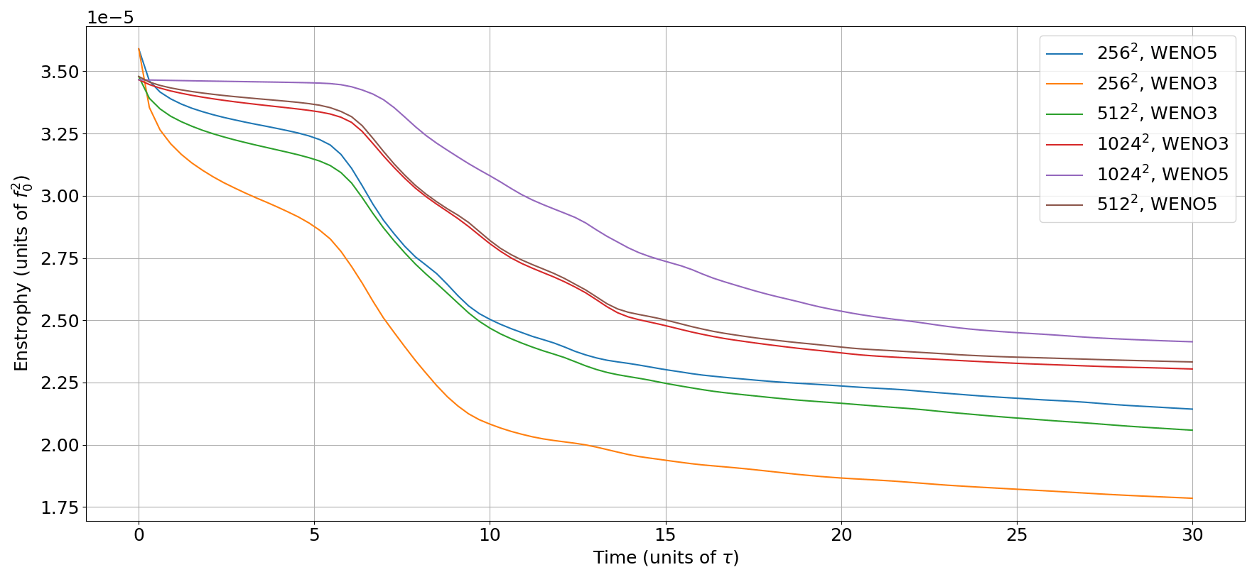
Figure 9Evolution of the total enstrophy for the vortex-shear at resolutions 10242, 5122, and 2562 using WENO-3 or WENO-5 for PV reconstruction.
To measure the sensitivity of our solver to the resolution and the order of the reconstruction scheme (3 or 5), we compare the solutions produced by our solver at resolutions 10242, 5122, and 2562 using third-order WENO (WENO-3) and fifth-order WENO (WENO-5) reconstructions. In Fig. 9 we plot the evolution of the total enstrophy at the three different resolutions. The results show that the enstrophy dissipation decreases as the resolution increases, indicating that a higher resolution better preserves the PV variance, and that low-resolution simulations suffer from an excessive dissipation.
We also note that WENO-3 leads to excessive numerical dissipation compared to WENO-5. Moreover, the enstrophy is better preserved with WENO-5 at resolution 5122 than with WENO-3 at resolution 10242. We plot in Fig. C1 in the Appendix the final state of the simulation at resolutions 5122 and 10242 with WENO-3 and WENO-5. This indicates that WENO-5 increases the effective resolution. In terms of computation cost, the simulation runtime is 1 min 2 s with WENO-5 at resolution 5122 and 5 min 52 s with WENO-3 at resolution 10242 with the NVIDIA RTX A3000 laptop GPU. This illustrates the benefits of using high-order reconstructions despite the fact that our code is globally second-order accurate.
5.2 Vortex–wall interaction
To challenge the numerics we now study the propagation of a single meso-scale vortex along a solid boundary, with a free-slip boundary condition. The domain is square with a thin-wall obstacle. Because the flow is inviscid, up to numerical errors, the vortex is expected to follow the boundary according to the mirror effect. In particular the vortex should slip around the obstacle and circumvent it, without detaching from it and without producing filaments (Deremble et al., 2016). The challenge is thus to have a solution that is as inviscid as possible and to enforce as much as possible both the no-flow and the free-slip boundary conditions.
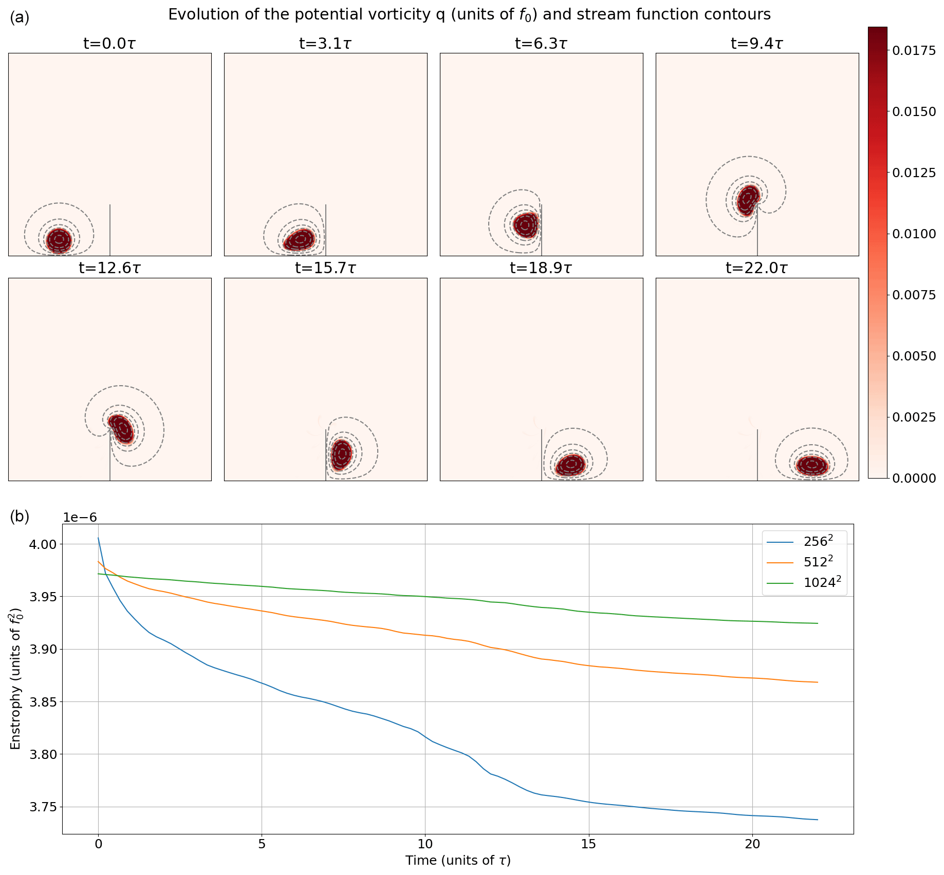
Figure 10Vortex–wall interaction experiment. (a) Vortex potential vorticity q and stream function ψ contours at initial time t=0; at intermediate times , and 18.9τ; and at final simulation time 22τ. (b) Evolution of the total enstrophy at resolutions 10242, 5122, and 2562.
The setup is as follows. The domain size is 100 km × 100 km on an f plane with a Coriolis parameter f0. The thin-wall obstacle is vertical, starting from the middle of the domain south boundary, and of length (see Fig. 10) and has a two-cell width. There is a single layer of fluid with reference thickness H=1 km. We assume no-flow and free-slip boundary conditions. The gravity constant is set to g=10 m s−2. In the initial state, the vortex is a circle of radius r0=10 km with constant PV and is at the bottom of the domain and at the left of the wall. The circular shape differs from the oval shape a vortex has when moving along a rectilinear wall. The remaining parameters of the simulation are set via the Rossby and Burger numbers with Ro=0.01, and Bu=1.
Figure 10 shows PV snapshots at various times, superimposed with the SF. The vortex behaves according to the inviscid regime. It clearly follows the wall and the obstacle elastically, without any sign of dissipative process such as filament detachment. The vortex at t=22 τ has recovered the characteristic oval shape. Between t=9.4 τ and t=12.6 τ, the vortex circumvents the edge, which causes it to experience its maximal deformation, but the solution remains smooth. The SF is clearly constant along the boundary, as a direct consequence of the capacitance matrix method. During the circumvention, it remains so, despite the thin wall imposing a strong curvature at the edge.
This experiment shows that the numerics has very good conservation properties on inviscid flows. This may come as a surprise since the upwinding does induce a numerical dissipation. In practice, the dissipation seems to self-adjust to the minimum required to prevent noise at the grid scale. This way of discretizing, in line with the ILES approach, turns out to be a viable alternative to conservative discretization combined with an explicit dissipation term.
At the bottom of Fig. 10 we plot the evolution of the total enstrophy at the three different resolutions. Once again, we note that the enstrophy dissipation decreases as the resolution increases: higher resolutions better preserve the PV variance, while low-resolution simulations suffer from more dissipation.
5.3 Double-gyre configuration
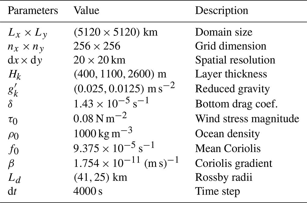
Our third numerical experiment to validate our solver is an idealized double-gyre configuration. Double-gyre configurations are a natural test for QG implementation or parameterization (e.g., Zanna et al., 2017; Ryzhov et al., 2020; Uchida et al., 2022). We consider here an octagonal ocean basin to illustrate the ability of our solver to handle non-square geometries. This octagon has maximal dimensions Lx×Ly. We assume free-slip boundary conditions on the boundaries. We consider N=3 layers on the vertical. We use an idealized stationary and symmetric wind stress (τx,τy) with and τy=0 on the top and linear drag at the bottom drag coefficient δ. The parameter values are given in Table 1.
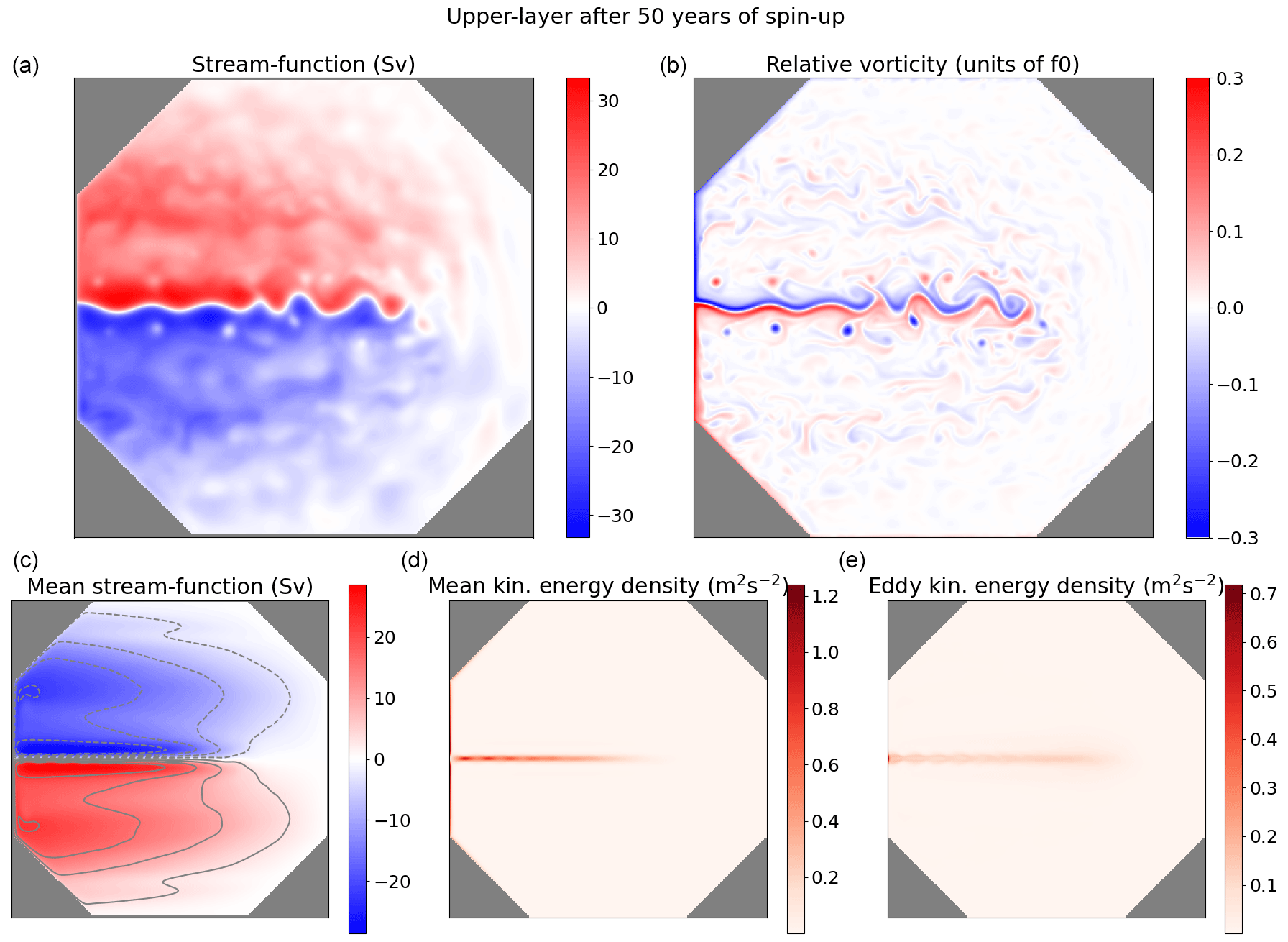
Figure 11(a, b) Upper-layer stream function ψ and relative vorticity (i.e., Δψ) after 50 years of spin-up. (c, d, e) Upper-layer mean stream function, mean kinetic energy density, and eddy kinetic energy density computed over 40 years after 10 years of spin-up.
We study this configuration in an eddy-permitting resolution of 20 km; the eddy-resolving meaning that the spatial resolution (20 km) is half of the larger baroclinic Rossby radius (41 km). Already at such eddy-permitting resolution, multi-layer QG solvers do not necessarily produce a well-pronounced eastward jet and usually require additional eddy parameterization (Uchida et al., 2022).
We plot at the top of Fig. 11 a snapshot of upper-layer SF and relative vorticity (i.e., Δψ) after 30 years of spin-up. As expected, our solver produces a strong western boundary current on the vertical and non-vertical boundaries. In the middle of this boundary starts a well-extended eastward jet whose length is qualitatively comparable with the Gulf Stream length in the North Atlantic basin. This jet is surrounded by a recirculation zone with several meso-scale eddies, which appears coherent with eddy-resolving-resolution simulations. We notice large-scale Rossby waves that are emerging near the eastern boundary and that propagate westward.
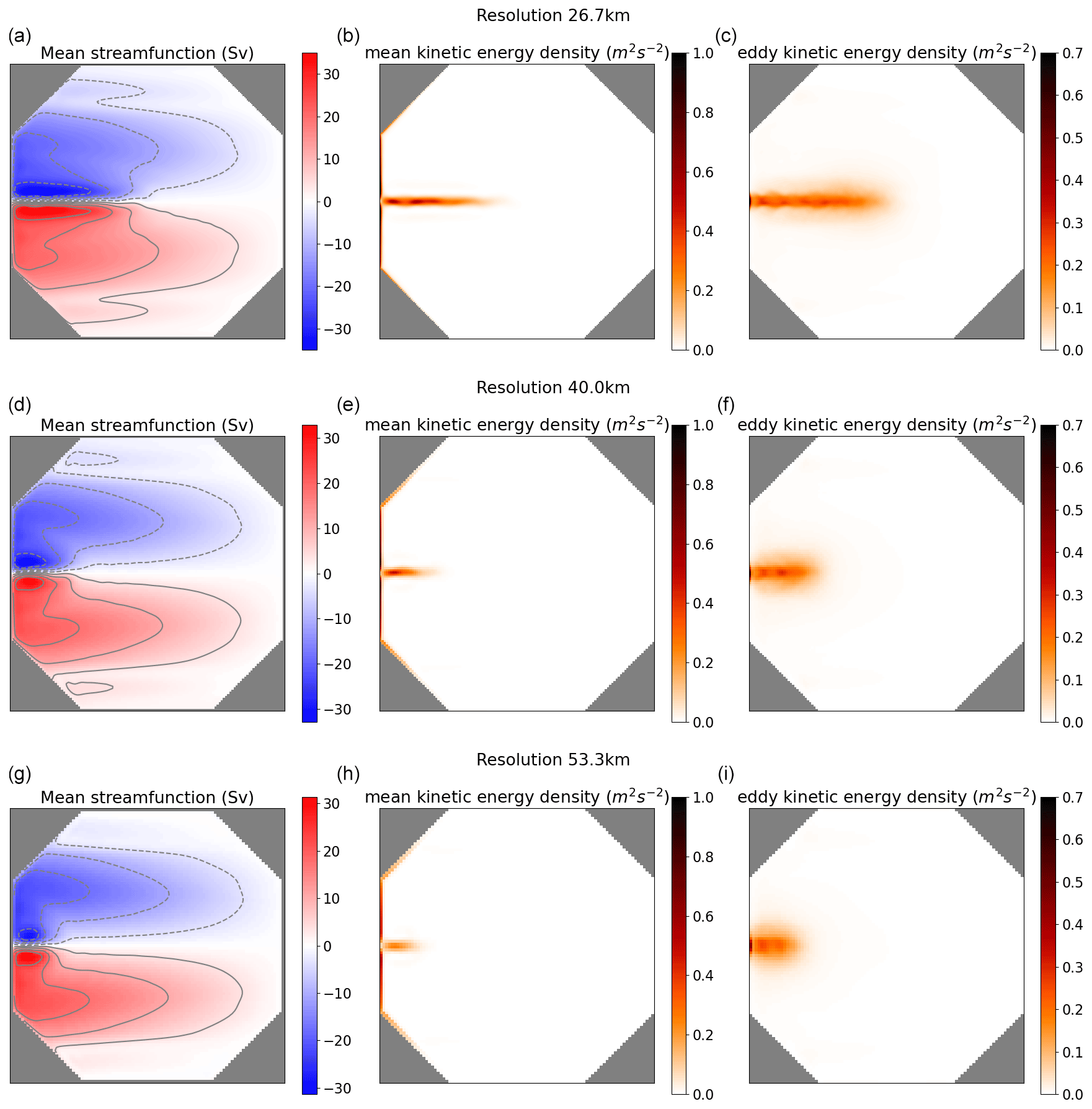
Figure 12Upper-layer mean stream function, mean kinetic energy density, and eddy kinetic energy density computed over 40 years after 10 years of spin-up at resolutions (top to bottom) 27, 40, and 53 km.
Since this system is chaotic, showing a snapshot is not very representative of the dynamical behavior of the system. We plot statistics of our solution at the bottom of Fig. 11: the mean SF, the mean kinetic energy (i.e., the kinetic energy of the mean velocity), and the eddy kinetic energy (i.e., the kinetic energy of the velocity standard deviation). These statistics were computed over 40 years after 10 years of spin-up, saving one snapshot every 15 years. These statistics are symmetric, which is expected since the domain shape and the wind forcing are symmetric. They confirm the presence of a strong western boundary current and fluctuating eastward jet whose length is roughly three-quarters of the domain. These results seem to confirm the relevance of implicit dissipation provided by upwinding, since usual multi-layer QG solvers require additional eddy parameterization (Uchida et al., 2022) to produce a well-pronounced eastward jet.
To assess the influence of the resolution on the solution produced by our solver, we run the same double-gyre experiment at lower resolutions: 27, 40, and 53 km. We plot the mean SF as well as the mean and eddy kinetic energy statistics in Fig. 12. We note that the eastward jet progressively diminishes as the resolution decreases: at resolution 27 km, it barely reaches the middle of the domain, while at resolutions 40 and 53 km, it almost disappears. At these two coarsest resolutions that are comparable to the largest baroclinic Rossby radius, 41 km in our configuration, meso-scale eddies cannot be resolved properly by our solver, and one would require an additional eddy parameterization to produce the eastward jet (Zanna et al., 2017).
We presented MQGeometry, a multi-layer quasi-geostrophic equation solver for non-rectangular geometries. This solver has three original aspects compared to usual solvers such as Q-GCM, PyQG, or PEQUOD: the use of finite volume for advection via staggering of the PV and SF, the non-linear WENO upwind-biased reconstructions with implicit dissipation, and the ability to handle non-square geometry with a fast spectral DST solver combined with the capacitance matrix method. Running a simulation with this solver does not require the tuning of any additional parameter, e.g., additional hyper-viscosity.
This multi-layer QG solver delivers a computationally efficient playground for studying meso-scale non-linear dynamics. It opens the way to study QG dynamics in basins with a realistic coastline, e.g., Mediterranean or North Atlantic basins. Moreover, with PyTorch automatic differentiation, one can easily build upon this implementation to develop new machine-learning parameterizations of the QG sub-grid scales or new data-assimilation techniques using QG.
We believe that more complex modeling systems can be implemented in high-level languages like Python without sacrificing performance, as demonstrated by Häfner et al. (2021). The QG system that we implemented in this solver is fairly simple, and the present solver should be seen as a proof of concept. Our plan is to extend the presented approach to shallow-water equations and subsequently to primitive equations. Major advantages are the seamless parallelism offered by GPUs, enabling us to write code that closely aligns with the continuous equations, and the automatic differentiation, allowing us to learn vertical parameterization in an end-to-end fashion (Kochkov et al., 2023).
One typically solves multi-layer QG equations using the strategy that follows (e.g., Hogg et al., 2014).
-
Use an evenly spaced Arakawa-C grid with the PV and the SF discretized on the same location, namely, the cell vertices (see left panel of Fig. 1).
-
Solve the PV advection Eq. (1a) using the energy–enstrophy-conservative Arakawa–Lamb scheme (Arakawa and Lamb, 1981) in the interior domain (i.e., not on the boundaries).
-
Since the scheme is energy conserving, use an additional (hyper-)viscosity scheme to dissipate the energy fueled by the wind forcing.
-
Given the matrix A diagonalization
where the layer-to-mode matrix Cl2m is the inverse of the mode-to-layer matrix Cm2l, and Λ is a diagonal matrix containing A eigenvalues, perform the following layer-to-mode transform:
With this transform, the elliptic Eq. (1b) becomes a stack of N two-dimensional Helmholtz equations
with homogeneous Dirichlet boundary conditions.
-
Solve these N two-dimensional Helmholtz equations, using, e.g., fast diagonalization with type-I discrete sine transform (DST-I):
-
Transform back from mode to layers
-
Update the PV boundary values using the elliptic Eq. (1b). This requires definition of the Laplacian on the boundaries and possibly involves partial free-slip/no-slip boundary conditions.
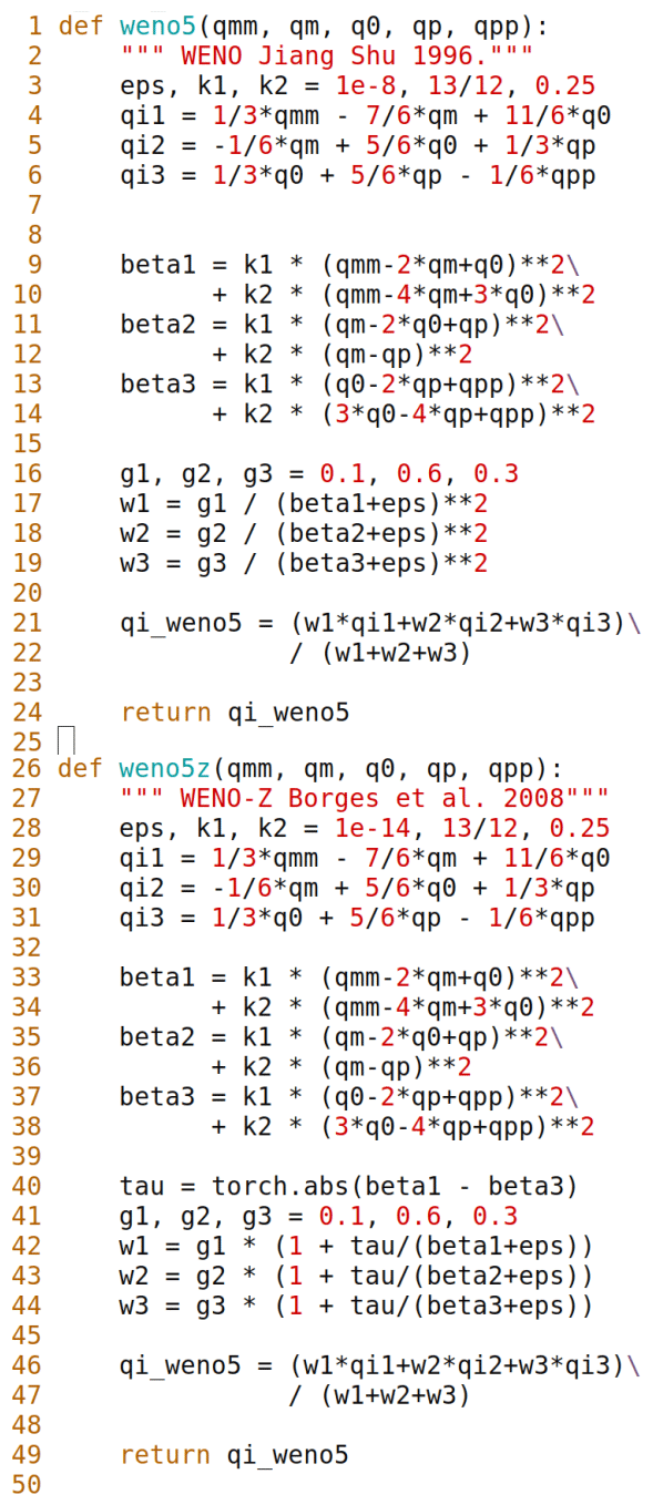
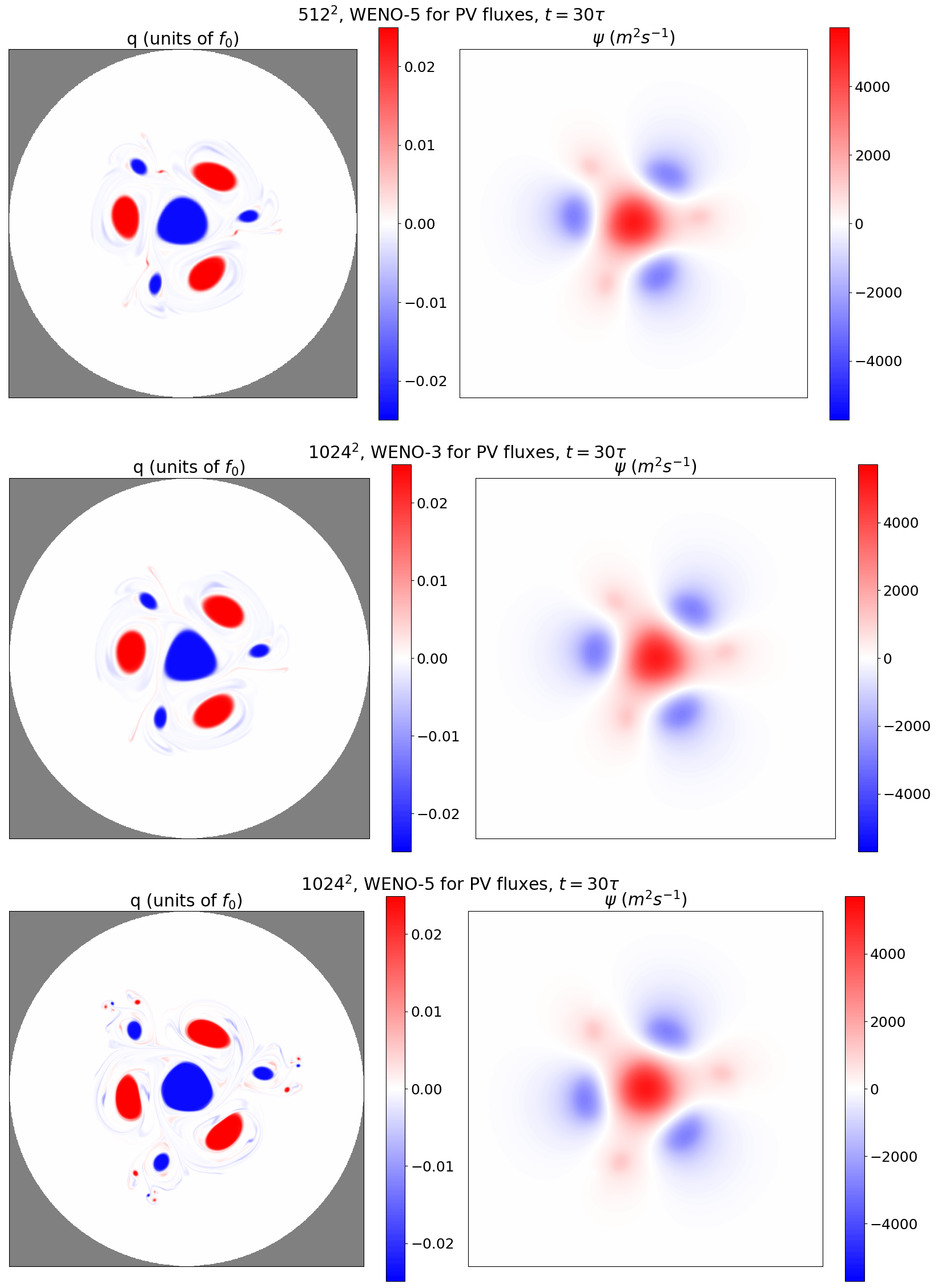
Figure C1Vortex-shear instability final state (t=30τ) with resolution 5122 and WENO-5 and with resolution 10242 and WENO-3/WENO-5.
The Python source code to reproduce the results is accessible on-line at https://github.com/louity/MQGeometry (last access: 26 February 2024) and https://doi.org/10.5281/zenodo.8364234 (Thiry, 2023). It contains a readme file with the instructions to run the code and a script to compute statistics and reproduce the figures. No data sets were used in this article.
LT implemented the PyTorch software, conducted the numerical experiments, and wrote the paper. GR gave the original idea of the staggering and the use of WENO, supervised the numerical experiments, and corrected the paper. LL helped with numerical experiments and paper revision. EM supervised the project.
The contact author has declared that none of the authors has any competing interests.
Publisher's note: Copernicus Publications remains neutral with regard to jurisdictional claims made in the text, published maps, institutional affiliations, or any other geographical representation in this paper. While Copernicus Publications makes every effort to include appropriate place names, the final responsibility lies with the authors.
The authors acknowledge the support of the ERC EU project 856408-STUOD. We would like to express our warm thanks to Laurent Debreu for pointing us to the capacitance matrix method. We also thank Nicolas Crouseilles, Pierre Navaro, Erwan Faou, and Georges-Henri Cottet for the amicable exchanges and interesting discussions.
This research has been supported by the European Research Council, H2020 European Research Council (grant no. 856408-STUOD).
This paper was edited by Deepak Subramani and reviewed by two anonymous referees.
Arakawa, A. and Lamb, V. R.: A potential enstrophy and energy conserving scheme for the shallow water equations, Mon. Weather Rev., 109, 18–36, 1981. a, b
Blayo, E. and LeProvost, C.: Performance of the Capacitance Matrix Method for Solving Helmhotz-Type Equations in Ocean Modelling, J. Comput. Phys., 104, 347–360, 1993. a
Borges, R., Carmona, M., Costa, B., and Don, W. S.: An improved weighted essentially non-oscillatory scheme for hyperbolic conservation laws, J. Comput. Phys., 227, 3191–3211, 2008. a, b, c, d
Boris, J. P., Grinstein, F. F., Oran, E. S., and Kolbe, R. L.: New insights into large eddy simulation, Fluid Dynam. Res., 10, 199, https://doi.org/10.1016/0169-5983(92)90023-P, 1992. a
Brown, N.: A comparison of techniques for solving the Poisson equation in CFD, arXiv [preprint], https://doi.org/10.48550/arXiv.2010.14132, 2020. a
Constantinou, N. C., Wagner, G. L., Siegelman, L., Pearson, B. C., and Palóczy, A.: GeophysicalFlows.jl: Solvers for geophysical fluid dynamics problems in periodic domains on CPUs & GPUs, J. Open Source Softw., 6, 3053, https://doi.org/10.21105/joss.03053, 2021. a
Deremble, B., Dewar, W. K., and Chassignet, E. P.: Vorticity dynamics near sharp topographic features, J. Mar. Res., 74, 249–276, 2016. a
Fox-Kemper, B., Bachman, S., Pearson, B., and Reckinger, S.: Principles and advances in subgrid modelling for eddy-rich simulations, Clivar Exchanges, 19, 42–46, 2014. a
Fulton, S. R., Ciesielski, P. E., and Schubert, W. H.: Multigrid methods for elliptic problems: A review, Mon. Weather Rev., 114, 943–959, 1986. a
Grinstein, F. F., Margolin, L. G., and Rider, W. J.: Implicit large eddy simulation, vol. 10, Cambridge university press Cambridge, https://doi.org/10.1017/CBO9780511618604. 2007. a
Häfner, D., Nuterman, R., and Jochum, M.: Fast, cheap, and turbulent – Global ocean modeling with GPU acceleration in python, J. Adv. Model. Earth Sy., 13, e2021MS002717, https://doi.org/10.1029/2021MS002717, 2021. a, b, c
Harten, A.: On a class of high resolution total-variation-stable finite-difference schemes, SIAM J. Numer. Anal., 21, 1–23, 1984. a
Hogg, A. M. C., Dewar, W. K., Killworth, P. D., and Blundell, J. R.: Formulation and users’ guide for Q-GCM, Mon. Weather Rev., 131, 2261–2278, https://doi.org/10.1175/1520-0493(2003)131<2261:AQCMQ>2.0.CO;2, 2014. a, b, c, d
Jiang, G.-S. and Shu, C.-W.: Efficient implementation of weighted ENO schemes, J. Comput. Phys., 126, 202–228, 1996. a, b, c, d, e
Kevlahan, N. K.-R. and Lemarié, F.: wavetrisk-2.1: an adaptive dynamical core for ocean modelling, Geosci. Model Dev., 15, 6521–6539, https://doi.org/10.5194/gmd-15-6521-2022, 2022. a
Kochkov, D., Yuval, J., Langmore, I., Norgaard, P., Smith, J., Mooers, G., Lottes, J., Rasp, S., Düben, P., Klöwer, M., Hatfield, S., Battaglia, P., Sanchez-Gonzalez, A., Willson, M., Brenner, M. P.,and Hoyer, S.: Neural General Circulation Models, arXiv [preprint], https://doi.org/10.48550/arXiv.2311.07222, 2023. a
Lemarié, F., Debreu, L., Madec, G., Demange, J., Molines, J.-M., and Honnorat, M.: Stability constraints for oceanic numerical models: implications for the formulation of time and space discretizations, Ocean Model., 92, 124–148, 2015. a, b
Li, L., Deremble, B., Lahaye, N., and Mémin, E.: Stochastic Data-Driven Parameterization of Unresolved Eddy Effects in a Baroclinic Quasi-Geostrophic Model, J. Adv. Model. Earth Sy., 15, e2022MS003297, https://doi.org/10.1029/2022MS003297, 2023. a
Liu, X.-D., Osher, S., and Chan, T.: Weighted essentially non-oscillatory schemes, J. Comput. Phys., 115, 200–212, 1994. a, b, c
Marshall, D. P., Maddison, J. R., and Berloff, P. S.: A framework for parameterizing eddy potential vorticity fluxes, J. Phys. Oceanogr., 42, 539–557, 2012. a
Morel, Y. G. and Carton, X. J.: Multipolar vortices in two-dimensional incompressible flows, J. Fluid Mech., 267, 23–51, 1994. a, b, c
Paszke, A., Gross, S., Massa, F., Lerer, A., Bradbury, J., Chanan, G., Killeen, T., Lin, Z., Gimelshein, N., Antiga, L., Desmaison, A., Kopf, A., Yang, E., DeVito, Z., Raison, M., Tejani, A., Chilamkurthy, S., Steiner, B., Fang, L., Bai, J., and Chintala, S.: Pytorch: An imperative style, high-performance deep learning library, arXiv [preprint], https://doi.org/10.48550/arXiv.1912.01703, 2019. a
Press, W. H. and Teukolsky, S. A.: Numerical recipes 3rd edition: The art of scientific computing, Cambridge university press, ISBN 9780521880688, 2007. a
Proskurowski, W. and Widlund, O.: On the numerical solution of Helmholtz’s equation by the capacitance matrix method, Math. Comput., 30, 433–468, 1976. a, b, c
Roullet, G., Mcwilliams, J. C., Capet, X., and Molemaker, M. J.: Properties of steady geostrophic turbulence with isopycnal outcropping, J. Phys. Oceanogr., 42, 18–38, 2012. a, b
Ryzhov, E., Kondrashov, D., Agarwal, N., McWilliams, J., and Berloff, P.: On data-driven induction of the low-frequency variability in a coarse-resolution ocean model, Ocean Model., 153, 101664, https://doi.org/10.1016/j.ocemod.2020.101664, 2020. a, b
Shu, C.-W. and Osher, S.: Efficient implementation of essentially non-oscillatory shock-capturing schemes, J. Comput. Phys., 77, 439–471, 1988. a
Thiry, L.: MQGeometry-1.0: a multi-layer quasi-geostrophic solver on non-rectangular geometries, Zenodo [code], https://doi.org/10.5281/zenodo.8364235, 2023. a
Uchida, T., Deremble, B., and Popinet, S.: Deterministic model of the eddy dynamics for a midlatitude ocean model, J. Phys. Oceanogr., 52, 1133–1154, 2022. a, b, c, d
Van der Vorst, H. A.: Bi-CGSTAB: A fast and smoothly converging variant of Bi-CG for the solution of nonsymmetric linear systems, SIAM J. Sci. Stat. Comput., 13, 631–644, 1992. a
Von Hardenberg, J., McWilliams, J., Provenzale, A., Shchepetkin, A., and Weiss, J.: Vortex merging in quasi-geostrophic flows, J. Fluid Mech., 412, 331–353, 2000. a, b
Zanna, L., Mana, P. P., Anstey, J., David, T., and Bolton, T.: Scale-aware deterministic and stochastic parametrizations of eddy-mean flow interaction, Ocean Model., 111, 66–80, 2017. a, b, c
- Abstract
- Introduction
- PV advection with finite volumes
- Spectral elliptic solver on non-rectangular domain
- Implementation
- Numerical validation
- Conclusions
- Appendix A: Usual discretization of multi-layer QG equations
- Appendix B: WENO implementation
- Appendix C: Vortex-shear instability
- Code and data availability
- Author contributions
- Competing interests
- Disclaimer
- Acknowledgements
- Financial support
- Review statement
- References