GPEP v1.0: the Geospatial Probabilistic Estimation Package to support Earth science applications

Ensemble geophysical datasets are foundational for research to understand the Earth system in an uncertainty-aware context and to drive applications that require quantification of uncertainties, such as probabilistic hydro-meteorological estimation or prediction. Yet ensemble estimation is more challenging than single-value spatial interpolation, and open-access routines and tools are limited in this area, hindering the generation and application of ensemble geophysical datasets. A notable exception in the last decade has been the Gridded Meteorological Ensemble Tool (GMET), which is implemented in FORTRAN and has typically been configured for ensemble estimation of precipitation, mean air temperature, and daily temperature range, based on station observations. GMET has been used to generate a variety of local, regional, national, and global meteorological datasets, which in turn have driven multiple retrospective and real-time hydrological applications. Motivated by an interest in expanding GMET flexibility, application scope, and range of methods, we have developed the Python-based Geospatial Probabilistic Estimation Package (GPEP) that offers GMET functionality along with additional methodological and usability improvements, including variable independence and flexibility, an efficient alternative cross-validation strategy, internal parallelization, and the availability of the scikit-learn machine learning library for both local and global regression. This paper describes GPEP and illustrates some of its capabilities using several demonstration experiments, including the estimation of precipitation, temperature, and snow water equivalent ensemble analyses on various scales.

1 Introduction

Meteorological datasets are essential for hydrometeorological and climate analysis and a wide range of related applications, from hydrometeorological forecasting to century-scale water security studies. Numerous gridded meteorological datasets exist based on a variety of estimation approaches, including the spatial interpolation of ground stations (Daly et al., 1994; Harris et al., 2020; Livneh et al., 2015; Maurer et al., 2002), remote sensing measurements from satellite sensors and weather radars (Huffman et al., 2007; Joyce et al., 2004; Shen et al., 2018; Zhang et al., 2016), and atmospheric and Earth system modelling (Gelaro et al., 2017; Hersbach et al., 2020; Kobayashi et al., 2015; Muñoz-Sabater et al., 2021). Among these datasets, those based on ground-station observations offer the most accurate meteorological records and are thus often used in the production of high-quality regional, national, and global gridded datasets. Station observations may be the sole input to the datasets, along with geophysical features that aid in a “smart interpolation” to account for terrain and other influences, or they may be used for bias correction of remote sensing and model estimates or as the calibration reference for multi-source merging (Baez-Villanueva et al., 2020; Beck et al., 2019; Sun et al., 2018).

Methods for the spatial interpolation of station observations range in complexity from simpler strategies, such as Thiessen polygons, distance-based weighting, linear interpolation, and nearest neighbour selection, to more complex procedures such as Kriging interpolation, geographically weighted regression (GWR), and machine learning techniques. Many widely used deterministic meteorological datasets are produced using these methods or their variants, such as the Global Precipitation Climatology Centre (GPCC) dataset (Schamm et al., 2014) and the Climatic Research Unit gridded Time Series (CRU TS) dataset (Harris et al., 2020). Yet spatial interpolation is an imperfect process that leads to ubiquitous uncertainties in gridded meteorological datasets. Few meteorological datasets provide explicit analytical uncertainty estimates, and even fewer provide probabilistic or ensemble estimates, members of which can be advantageous in quantifying uncertainties and characterizing extreme events (Tang et al., 2023). To address this problem, several recent studies have developed station-based ensemble meteorological datasets, including the Hadley Centre/Climate Research Unit Temperature version 4 (HadCRUT4) global temperature dataset (Morice et al., 2012), the Spatially COherent Probabilistic Extended Climate dataset (SCOPE Climate) in France (Caillouet et al., 2019), the ensemble precipitation and temperature datasets in the United States and parts of Canada (Newman et al., 2015, 2019, 2020), the Ensemble Meteorological Dataset for North America (EMDNA; Tang et al., 2021a), and the Ensemble Meteorological Dataset for Planet Earth (EM-Earth; Tang et al., 2022). Several deterministic datasets such as the Europe-wide E-OBS (Haylock et al., 2008; Cornes et al., 2018) and Canadian Precipitation Analysis (CaPA; Mahfouf et al., 2007; Fortin et al., 2015; Khedhaouiria et al., 2020) also offer probabilistic realizations. In addition to these station-based datasets, there are also reanalysis ensembles such as ERA5 Ensemble of Data Assimilations (Hersbach et al., 2020) and satellite-based ensemble generation methods such as the satellite rainfall error model (Hossain and Anagnostou, 2006; Hartke et al., 2022), which are beyond the scope of this study.

However, the rise of ensemble meteorological datasets also brings new challenges or amplifies existing ones. First, like many other historical datasets, ensemble datasets are often built on open-access station collections, with fixed periods and resolutions and limited variables, which may not be updated routinely once the production is finished. Second, ensemble datasets often have large data sizes increasing with the number of members, posing challenges in downloading, storage, and processing. Third, ensemble estimation methods generally have much higher complexity compared to single-value spatial interpolation methods, making it difficult for researchers and practitioners to produce their datasets following dataset and method description publications. Therefore, open-access tools for creating ensemble meteorological datasets are equally important and sometimes more useful to the community compared to public datasets. Several such spatial interpolation tools are available in various stages of development, such as the Topographically InformEd Regression (TIER; Newman and Clark, 2020), GStatSim (MacKie et al., 2022), TFInterpy (Chen and Zhong, 2022), and multiscale GWR (MGWR; Oshan et al., 2019), but well-tested tools for meteorological ensemble estimation remain rare. A notable exception is the Gridded Meteorological Ensemble Tool (GMET: https://github.com/NCAR/GMET, last access: 7 February 2024) which can be used to generate ensemble meteorological analyses (i.e., gridded surface forcings) using the locally weighted spatial regression method outlined in Clark and Slater (2006). After an initial FORTRAN development effort (Newman et al., 2015), GMET has been further refined and expanded in the course of sequential application projects, producing a number of regional to continental datasets (Bunn et al., 2022; Liu et al., 2022; Longman et al., 2019; Newman et al., 2015, 2019, 2020; Wood et al., 2021a).

Successful GMET applications to date motivated interest in enhancements to allow for a broader range of uses and available methods. GMET's FORTRAN basis enables it to be computationally efficient and fast but is more cumbersome for adding or linking to new methodological modules than the widely used scripting and programming language Python, for which many relevant method libraries exist, particularly including machine learning (ML) techniques. In addition, GMET's development to date has only afforded a subset of the potential user control over implementation choices, and some settings that would be required for more flexible implementation are currently hardwired. For instance, the most common application is to generate ensembles of precipitation, mean air temperature, and air temperature range; and certain assumptions, functions, and settings specific to precipitation and temperature must be changed in the code if other variables are of interest. Future development to enhance the FORTRAN GMET toward greater flexibility and user control is a viable option, but we view Python as providing a more convenient and extensible development environment and one that can engage a potentially larger community of contributors. The major downside of pursuing future development in Python relative to FORTRAN is its relatively slower computational speed, a tradeoff that we view as being acceptable given the benefits.

We have thus developed the Python-based Geospatial Probabilistic Estimation Package (GPEP). GPEP includes and expands upon most of the current functionalities of FORTRAN GMET, bringing new methodological and usability enhancements. These include (1) a flexible and configurable user control for input/output variables, run parameters, predictors, and weight functions; (2) options for using basic ML techniques for local and global regression; (3) an alternative, efficient approach for cross-validation; and (4) more flexible input formatting, especially for dynamic gridded predictor inputs. GPEP draws from and formalizes some functions that were previously applied in the production of the continental EMDNA (Tang et al., 2021a) and the global EM-Earth (Tang et al., 2022) datasets, while mimicking GMET functionality (such as cross-validation and usage of both static and time-variant predictor information) from Bunn et al. (2022).

GPEP is a powerful tool for both research and applications of deterministic and ensemble distributed geophysical analysis estimation, including the production of meteorological datasets to support retrospective and real-time modelling on various scales. This paper summarizes the GMET methodology and GPEP enhancements and illustrates some of its capabilities using several experimental applications.

2 Probabilistic estimation methodology

2.1 The theory of GMET

The core GMET methodology for probabilistic meteorological ensemble analyses assumes that the estimate of a meteorological variable at a specific time and location can be described by a parametric probability distribution. For mean air temperature and daily temperature range (i.e., the difference between maximum and minimum daily temperature), the normal distribution is used by GMET in the form of $X\sim N(\mathit{\mu },{\mathit{\sigma }}^{\mathrm{2}})$, where μ and σ are the mean value and standard deviation, respectively. μ represents the deterministic estimation of a variable, and σ represents the uncertainty of the μ estimation. Ensemble estimates can be obtained by sampling from the normal distribution. For variables such as precipitation with skewed distributions, transformation methods such as Box–Cox are applied to convert variables into normal (Gaussian) space. Although the GMET methodology was originally developed for precipitation and temperature estimation, it can also be applied to any variable that can be described using the normal distribution, either directly or through transformation.

2.2 Deterministic estimation

The premise of probabilistic estimation is obtaining μ and σ parameters. GMET adopts the locally weighted linear regression (LWLR) to obtain deterministic gridded estimates of μ. Let x_o be the raw or transformed station observation, then the LWLR estimate $\widehat{x}$ for the target point and time step is obtained as below:

$$\begin{array}{}\text{(1)}& x_{\mathrm{o}}=\widehat{x}+\mathit{\epsilon }={\mathit{\beta }}_{\mathrm{0}}+\sum _{i=\mathrm{1}}^n{A}_i{\mathit{\beta }}_i+\mathit{\epsilon },\end{array}$$

where A_i is the ith predictor, β₀ and β_i are regression coefficients, and ε is the residual (or error term). The initial implementation uses static terrain-related predictors such as latitude, longitude, elevation, topographic slope, and aspect (as in Clark and Slater, 2006, and Newman et al., 2015). GMET version 2.0 added the ability to use time-varying dynamic predictors such as precipitation and temperature from atmospheric models to further improve the accuracy of gridded estimates (Bunn et al., 2022).

To estimate σ, GMET version 2.0 also implemented k-fold cross-validation (including leave-one-out, LOO, as a particular case), which enables the use of predictive rather than calibration uncertainty in ensemble generation and provides an invaluable method for predictor screening and selection. σ is the uncertainty of gridded regression estimates μ based either on the standard error of the regression or the prediction error (e.g., root mean squared error from cross-validation).

In addition to μ and σ, for intermittent variables like precipitation, the probability of an event is required to determine whether an event occurs or not. GMET uses a locally weighted logistic regression to estimate the probability of precipitation (POP) to enable its probabilistic estimation: that is, the binary probability of the event (0 or 1) is regressed against the static and/or dynamic predictors (Eq. 2), which are also used in a precipitation amount regression. This method can be applied to other intermittent geospatial variables.

$$\begin{array}{}\text{(2)}& \text{POP}={\displaystyle \frac{\mathrm{1}}{\mathrm{1}+\exp (-{\mathit{\beta }}_{\mathrm{0}}+{\sum }_{i=\mathrm{1}}^n{A}_i{\mathit{\beta }}_i)}}\end{array}$$

While GMET employs locally weighted linear/logistic regression for its deterministic estimation, this component within the probabilistic estimation framework is method agnostic. It is designed to be compatible with a variety of geospatial estimation methods, a versatility that has been realized in GPEP.

2.3 Probabilistic estimation

GMET generates distributed, spatiotemporally correlated random fields (SCRFs) that are used to sample the distributed regression models, generating ensembles that each maintain the spatial and temporal correlation structures of the input variables (Newman et al., 2015). For SCRF, the spatial correlation length (C_len) is used to represent the spatial correlation structure over the entire domain:

$$\begin{array}{}\text{(3)}& c_{i,j}=\exp \left(-{\displaystyle \frac{d_{i,j}}{C_{\text{len}}}}\right),\end{array}$$

where d_i,j is the distance between grids i and j, and C_len is the spatial correlation length determined for each variable using station data. The random number for a given target grid point is conditioned based on previously generated points, utilizing a nested simulation strategy to enhance calculation efficiency. Please refer to Clark and Slater (2006) for more details.

The temporal correlation structure is represented using the lag-1 auto-correlation of a variable to link the SCRF at two consecutive time steps. In addition, if a variable shows a dependent relation with another variable, the cross-correlation between the two variables can be used to correlate their SCRFs. For GMET, the lag-1 auto-correlation of temperature and the cross-correlation between precipitation and daily temperature range are used to represent the temporal correlation structure and intervariable relationship (Eq. 4).

$$\begin{array}{}\text{(4)}& \left\{\begin{array}{l}{R}_{t,\text{T}}={\mathit{\rho }}_{\text{lag-1}}{R}_{t-\mathrm{1},\text{T}}+\sqrt{\mathrm{1}-{\mathit{\rho }}_{\text{lag-1}}^{\mathrm{2}}}{R}_{t-\mathrm{1},\text{T}},\\ R_{t,\text{P}}={\mathit{\rho }}_{\text{cross}}{R}_{t,\text{TR}}+\sqrt{\mathrm{1}-{\mathit{\rho }}_{\text{cross}}^{\mathrm{2}}}{R}_{t-\mathrm{1},\text{P}},\end{array}\right.\end{array}$$

where t and t−1 are the current and previous time steps, respectively. R_T, R_TR, and R_P are two-dimensional SCRFs of mean air temperature, and precipitation, respectively. ρ_lag-1 is the lag-1 auto-correlation of temperature. ρ_cross is the cross-correlation between precipitation and daily temperature range. For t=0, the SCRF is generated for each variable based only on the spatial correlation structure. The spatial correlation length, ρ_lag-1, and ρ_cross can be estimated from station observations.

After obtaining μ, σ, the POP, and SCRF, GMET can generate any number of ensemble members. Let R be the random number from the SCRF for a specific location and time step, the probabilistic estimate (x_T) for temperature variables can be obtained using the temperature uncertainty σ_T to perturb the deterministic temperature estimation μ_T (Eq. 5). The number of R or SCRFs is the number of ensemble members.

$$\begin{array}{}\text{(5)}& x_{\mathrm{T}}={\mathit{\mu }}_{\mathrm{T}}+R\cdot {\mathit{\sigma }}_{\mathrm{T}}\end{array}$$

For precipitation, non-zero values are generated in proportion to the POP. Let F_N(y) be the cumulative density function (CDF) of the standard normal distribution, and F_N(R) is the cumulative probability corresponding to the random number R. Note that y is precipitation undergoing the Box–Cox transformation (Sect. 2.1). Let p₀ be the POP for a specific location and time step; for an ensemble member, a precipitation event occurs only when F_N(R) is larger than p₀. If an event occurs, we need to calculate the scaled cumulative probability of precipitation (p_cs):

$$\begin{array}{}\text{(6)}& p_{\text{cs}}={\displaystyle \frac{F_{\mathrm{N}}\left(R\right)-p_{\mathrm{0}}}{\mathrm{1}-p_{\mathrm{0}}}}.\end{array}$$

The probabilistic estimate of precipitation is expressed similarly to Eq. (5) using the precipitation uncertainty σ_P to perturb the deterministic precipitation estimation μ_P:

$$\begin{array}{}\text{(7)}& y=\left\{\begin{array}{ll}\mathrm{0}& \text{if }{F}_{\mathrm{N}}\left(R\right)\le p_{\mathrm{0}},\\ {\mathit{\mu }}_{\mathrm{P}}+F_{\mathrm{N}}^{-\mathrm{1}}\left(p_{\text{cs}}\right)\cdot {\mathit{\sigma }}_{\mathrm{P}}& \text{if }{F}_{\mathrm{N}}\left(R\right)>p_{\mathrm{0}},\end{array}\right.\end{array}$$

where y is the precipitation in the normal space and $F_{\mathrm{N}}^{-\mathrm{1}}\left(p_{\text{cs}}\right)$ is the random value corresponding to p_cs. y is back-transformed to obtain the final precipitation values (x_P).

Details of the GMET methodology are introduced in previous development and dataset studies (e.g., Clark and Slater, 2006; Newman et al., 2015; Tang et al., 2021a; Bunn et al., 2022). Although Eqs. (5)–(7) are implemented for precipitation and temperature in GMET, the probabilistic estimation theory is generic and applicable to other variables.

3 GPEP

GPEP offers both methodological (Table 1) and usability (Table 2) features that expand on GMET, and these are described in Sect. 3.1 and 3.2, respectively. Like many software tools, GMET was first written for a specific application, and a key motivation for GPEP was to generalize a number of the hard-coded options to enable broader usage. Figure 1 shows the schematic of GPEP. A GPEP case is controlled by configuration files, with several templates available in the package. Once set up, GPEP engages in two key processes: (1) probabilistic estimation model fitting, corresponding to outputs from Sect. 2.2, and (2) ensemble generation, corresponding to outputs form Sect. 2.3.

Table 1 Comparison of GPEP and GMET methodological features.

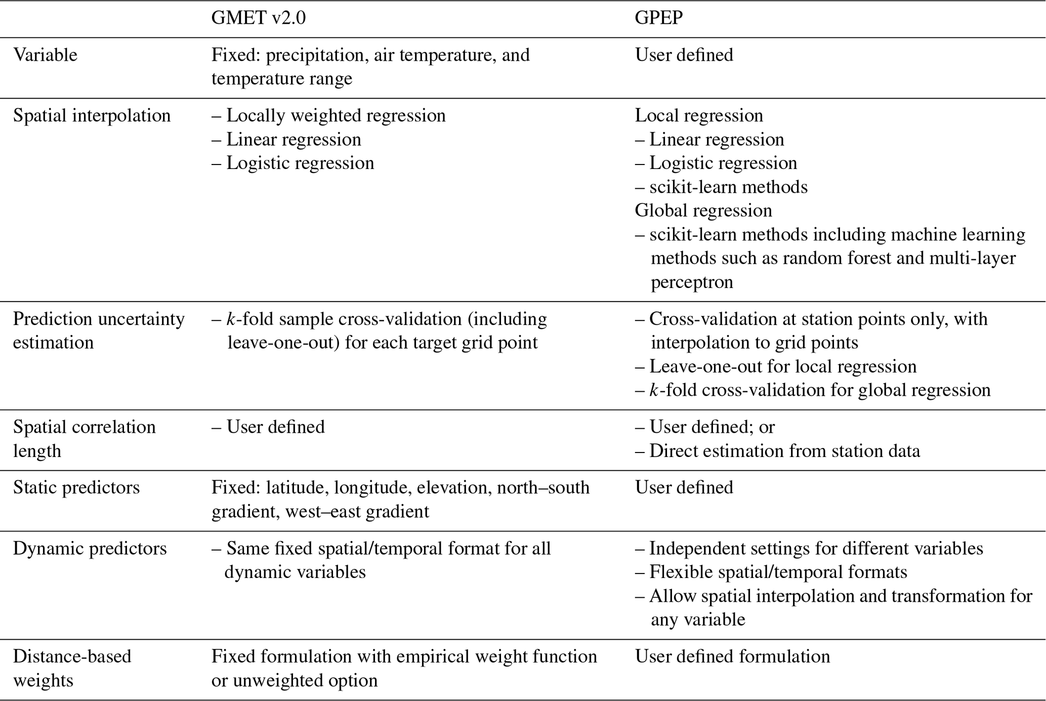
Table 2 Comparison of GPEP and GMET usability and technical features.

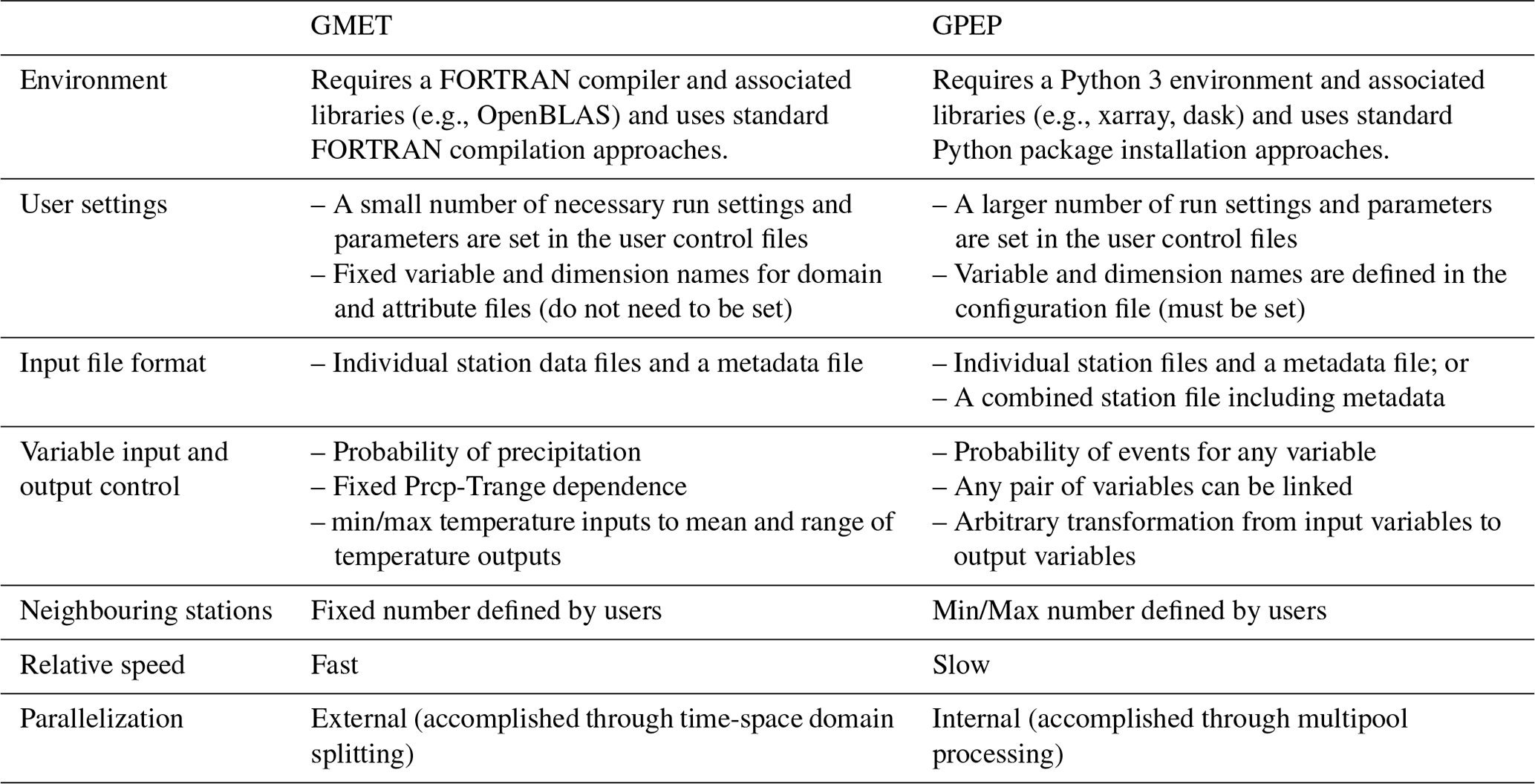
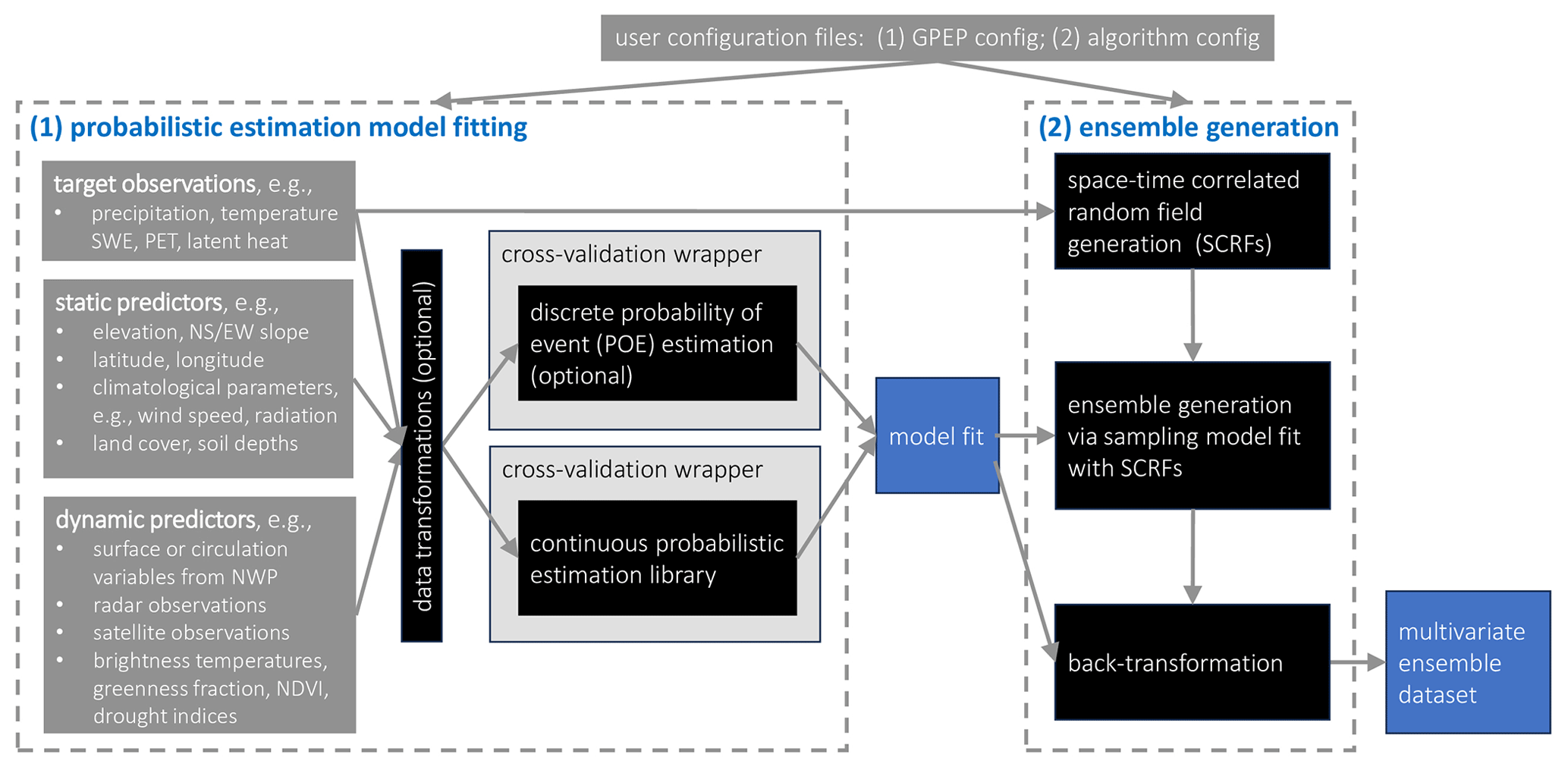
Figure 1 The schematic of GPEP. To set up a GPEP case, users first need to prepare configuration files based on the templates provided in the package. The GPEP will then implement (1) probabilistic estimation model fitting, which can also output deterministic geospatial estimates, and (2) ensemble generation of any number of members.

3.1 Methodological improvements

Here we introduce some major methodological improvements of GPEP compared to GMET. These changes enhance GPEP's flexibility as a tool not only for dataset production but also for scientific research aimed at achieving higher estimation accuracy or comparing the performance of different methodological strategies.

Variable selection flexibility

The original GMET code was implemented to estimate precipitation, mean daily air temperature (Tmean), and daily temperature range (Trange), although it has also been used to estimate only precipitation. The spatial regression method and design, however, are applicable to arbitrary spatiotemporal variables; thus, GPEP brings the variable selection and associated details into the user control (“configuration”) file. This versatility enables GPEP to generate ensemble analyses for other variables; in the Earth science or geophysical context, these might include other meteorological variables such as radiation, wind speed, humidity, and air pressure, which are commonly required for hydrological models, or even hydrological variables for which observations or other analyses exist, such as snow water equivalent (SWE).

Spatial interpolation

GMET supports only locally weighted linear and logistic regression, whereas GPEP expands the options beyond these two basic capabilities to also support any supervised learning method from the scikit-learn package (Pedregosa et al., 2011) that can use the fit function to train the model and use the predict/predict_proba to predict the output. Such techniques include ridge regression and classification, BayesianRidge regression, Lasso regression, and ElasticNet regression (among others) for locally weighted regression and regressors and classifiers of random forest (RF), multi-layer perceptron, and support vector machine (among others) for global regression. Global regression builds one model for the entire study domain at every time step, which is far more efficient than the local regression methods, whereas users need to caution that global regression may have degraded accuracy compared to local regression which needs in-depth investigation for case studies. Users can define the method for continuous and classification regression and define model parameters following scikit-learn formats in the configuration file.

Uncertainty estimation

GMET has the option to use a standard k-fold cross-validation to obtain the uncertainty of each grid cell specific regression estimate, where the number of folds is specified by the user. The use of k-fold cross-validation increases the computational demand in proportion to the number of folds, which was feasible in GMET but is not in GPEP, due to its slower speed and relatively costlier operation. Consequently, GPEP adopts an alternative cross-validated uncertainty estimation strategy: (1) obtaining regression estimates at all station points, using leave-one-out validation for local regression and N-fold cross-validation for global regression; and (2) interpolating the resulting root mean square error from the station points to each grid cell using a distance weighted (i.e., locally weighted) averaging. The GPEP method achieves generally similar uncertainties with the standard method at less computational cost. The similarity of the two error estimation outcomes, however, will depend on the nature of the station and grid datasets being used.

Spatial correlation length

This parameter is critical for generating SCRFs for ensemble member generation. GMET requires prescribed length values, whereas GPEP supports either user-specified correlation lengths or a data-driven option, in which the length is inferred from raw station inputs. Users can also set various thresholds for the correlation calculation. For example, a positive threshold such as 10 mm d⁻¹ can be used to focus only on heavy precipitation. With the data-driven option, users need to ensure that the input data length is enough for robust estimation of the correlation; the prescribed option is useful for smaller datasets (such as an operational forecast application) that are inadequate to define such correlation lengths.

Static and dynamic predictors

GMET uses a fixed grid for both the static and dynamic predictors, has a hard-coded default list of static predictors, and uses the same predictors for all target variables (with a minor exception of dropping slope from low-relief prediction situations, the threshold for which is also hard-coded). In contrast, GPEP allows users to define the static and dynamic predictors used for different target variables. GPEP supports the regridding and transformation of dynamic input data as well.

Distance-based weight

GMET v2.0 calculates local weights for the regression using a hard-coded exponential function based on the distance between two points, or allows for unweighted regression, and these choices can have a strong influence on regression estimation. GPEP more generally supports any user-defined distance functions based on the two parameters: dist (distance between points) and maxdist (max distance in weight calculation). This feature facilitates research on the impact of weight functions on regression and ensemble generation performance.

3.2 New technical and usability features in GPEP

GPEP has a different code design compared to GMET, leveraging features of Python to facilitate its implementation, debugging, and future improvement. A key consideration in the design of GPEP was providing backward compatibility with most input and run mode configuration features of GMET, to ease user transition and facilitate intercomparison.

Environment

The FORTRAN-based GMET has certain prerequisites in terms of computational environment, such as the availability of a FORTRAN compiler and libraries to support NetCDF file standards and linear algebra libraries (e.g., OpenBLAS). GPEP relies on the installation of at least Python 3, along with Python packages including scikit-learn, scipy, xarray, and dask. Whether GMET or GPEP is more accessible for a user will depend on the user's familiarity and facility with FORTRAN-related or Python-related computational dependencies. In general, both GMET and GPEP are designed with the use of common and/or open-source dependencies. Given the increasing prevalence of Python usage in the Earth science community, however, we believe that shifting future GMET development to a Python foundation will foster broader engagement by users and developers from more varied computational backgrounds.

User control

As is common with all models and software, GMET has a mixture of hard-coded settings or parameters and those that are exposed in configuration files to give the user control over the GMET application. As it has developed, more parameters have been exposed to increase GMET flexibility, and with GPEP we accelerate this trend, either through bringing parameters of interest into the user control file or providing more methodological options. Examples include the spatial correlation length for Tmean and Trange or Box–Cox transformation exponent. The GPEP user can specify (in the configuration file) previously fixed implementation details such as the names of the input dataset dimensions and static predictor variable names (e.g., “elevation”). Although not strictly necessary for GMET and GPEP operation, these settings allow the user to avoid pre-processing inputs to exacting formats and may enhance the tool's usability.

Input station data file format

GMET was coded to read station data time series from individual files, along with a single *.CSV metadata file, whereas GPEP can either use this input file organization or a single netCDF file that combines all stations and their metadata attributes. The latter approach may be more convenient for users who prefer to bundle the station time series into a single file, and the single self-documenting file is faster to read than individual files. It may be less convenient if the station dataset changes frequently (either in the number of stations or length). If used with individual station data files, GPEP will write a merged NetCDF station file to provide the user with both options on subsequent runs.

Input and output variable specifications

GMET is currently coded for its most common application, i.e., reading precipitation and temperature extrema (minimum and maximum) and writing precipitation and temperature mean and range (over the time step), which are estimated as the mean and difference of the extrema, respectively. For many daily meteorological applications, these are the most widely available and used variables. For ensemble member generation, the SCRFs of precipitation and temperature are explicitly linked (via cross-correlation). One of the most important new features of GPEP is to generalize GMET to allow the user to specify arbitrary input and output variables and linkages and transformations between them. In the configuration file, arithmetic expressions can be used to convert input variables to output variables, and the concept of POP is generalized to “probability of event” (POE), which can be estimated for any variable and can also use a user-defined event threshold. Users can also define the interdependence of variables in the ensemble generation step directly in the configuration file.

Neighbouring stations

GMET allows users to define a fixed number of neighbouring stations used in local regression, while GPEP allows users to define the minimum and maximum numbers of neighbouring stations. This feature responds to the reality that for large domains users may want to use different numbers of neighbouring stations for areas with different station densities. For example, it may be optimal to use fewer neighbouring stations in remote areas (e.g., northern Canada) to avoid involving stations without notable correlation to the target point, while more neighbouring stations can be used in densely gauged areas (e.g., the eastern USA).

Reproducibility and random field output

GMET by default uses a random seed when generating ensemble output, whereas GPEP gives users the option to fix (set) the seeds that control the random processes, such as SCRF generation and machine learning initial states. Fixing the random seeds will obtain the same ensemble outcomes from each GPEP run, enabling reproducibility that can be useful in debugging and development. GPEP also provides users with an option to output SCRF values, which may be of interest in development or for certain applications.

Parallelization

Computational efficiency is critical for operational application. Python is inherently slower than FORTRAN for many operations, and GPEP's production of ensemble analyses overall appears to be between 10 and 50 times slower than GMET, based on exploratory benchmarking. For instance, Python is around 10 times slower than FORTRAN for least-square linear regression functions. For complex computations and loops, the speed gap could be larger. Thus, we have parallelized GPEP's most time-consuming parts using the multiprocessing package to improve its speed (future versions may use other packages such as dask). To demonstrate the parallel efficiency, we tested two locally weighted regression methods (LWR: LWR1 and LWR2) and a global regression method (i.e., RF) for the GMET version 2.0 test case of daily meteorological forcing generation for February 2017 in California, USA (Bunn et al., 2022). Figure 2 shows that the default LWR1 functions are faster than LWR2, but both methods are slower than the global regression method RF. LWR2 is slower than LWR1 due to multiple factors, including the complexity and overhead of scikit-learn and the implementation difference (LWR1 is translated from FORTRAN codes using lower–upper decomposition). We observed a significant speedup for LWR1/LWR2 when CPUs increased from 1 to 25 and for RF when CPUs increased from 1 to 15. The speedup for RF diminishes because the compute time is relatively short for lower numbers of CPUs. The number of valid grids for this experiment is 12 419, based on which users may have a rough estimate of local regression time for their own LWR experiments. For generating ensemble members, parallel efficiency remains high with increasing CPU numbers up to 35, as different ensemble members can be generated simultaneously and can fully utilize the available CPUs.

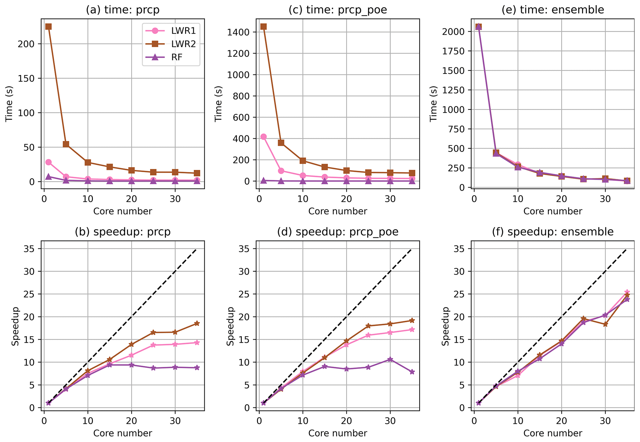
Figure 2 The CPU scaling of the time cost (a, c, e) and speedup (b, d, f) of precipitation (prcp) regression (a, b), the probability of event for precipitation (prcp_poe) regression (c, d), and the generation of 100 ensemble members (e, f). LWR1 represents the default GMET method using locally weighted linear and logistic regression. LWR2 represents scikit-learn's ridge regression and logistic regression, and RF represents the random forest regressor and classifier. Speedup is the ratio between compute time with 1 CPU versus with multiple CPUs.

3.3 GPEP documentation and applicability

GPEP comes with extensive documentation that is available on the GitHub repository and provides detailed information on how to set up the environment and prepare the configuration file and run GPEP. The documentation includes a comprehensive list of all the available parameters and options that can be used to customize the GPEP input and output (i.e., the ./docs/How_to_create_config_files.md). A Jupyter Notebook is provided, demonstrating the downloading and running of test cases (i.e., the ./docs/GPEP_demo.ipynb). The test cases are available at https://doi.org/10.5281/zenodo.8222852 (Tang and Wood, 2023b).

4 Demonstration experiments

We demonstrate a subset of GPEP capabilities through a small number of experiments described in this section. The first (Sect. 4.1) compares GPEP outcomes to those of GMET for the primary GMET test case, a 0.0625^∘ resolution daily meteorological ensemble generation for California, that is included in the GMET version 2.0 repository (Bunn et al., 2022). The second demonstration (Sect. 4.2) is for meteorological ensembles in a higher resolution (0.01^∘ or approximately 1 km) domain including the US Rocky Mountain headwaters of the Colorado Headwaters; the third (Sect. 4.3) illustrates the use of GPEP to generate ensemble analyses of SWE for the same domain.

4.1 GMET and GPEP comparison

In this experiment, we compared the outputs of GPEP and GMET using the GMET version 2.0 test case in California, USA. Figure 3 depicts the agreement between the GMET and GPEP regression model mean estimation of the four primary GMET output variables, focusing on the locally weighted linear and logistic regression method based on static predictors only. For precipitation, Tmean, and Trange, the GPEP and GMET estimates are almost identical for all samples, with the data pairs for all time steps and grid cells in the domain mainly located along the 1–1 line. For Tmean and Trange, some subtle differences within ±0.1 ^∘C are observed in the eastern parts of the domain. The minor discrepancies, especially in the probability of precipitation, come from slight numerical differences in data inputs, attributed to differences in double precision or single precision in GPEP and GMET codes. These minor variations can be magnified during iterative processes of logistic regression. GPEP tends to generate lower precipitation POE than GMET for low precipitation probability, while for high POE GPEP generates higher probabilities. The positive and negative differences do not show observable spatial patterns. In general, GPEP's mean precipitation POE is slightly higher than that of GMET by 0.005 (∼1 %), which is negligible.

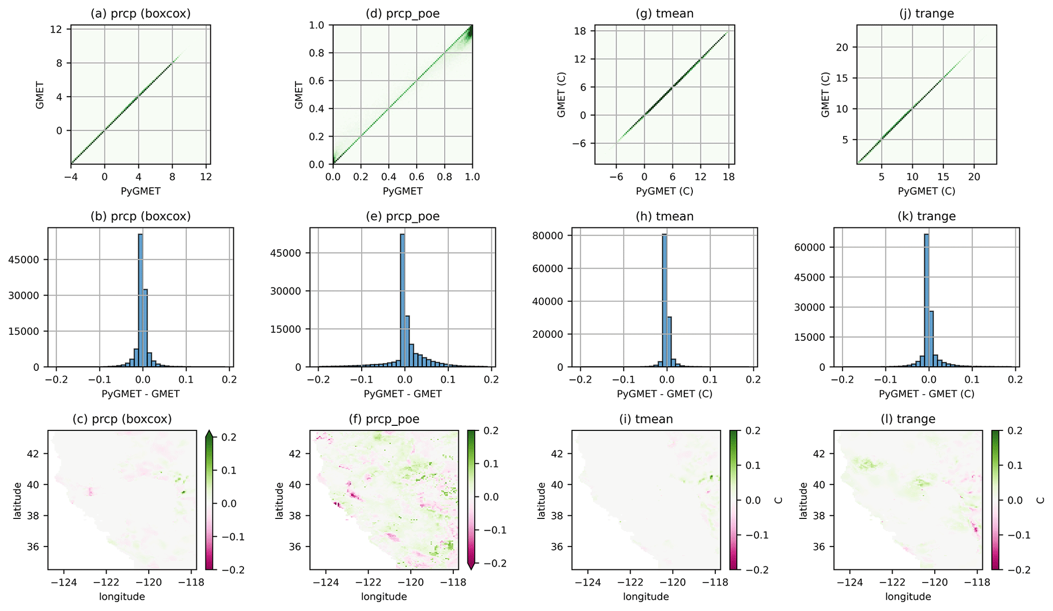
Figure 3 The scatter density plots (first row) between GPEP and GMET estimates of precipitation (prcp) after Box–Cox transformation with a minimum value of −4, precipitation probability of the event (prcp_poe), mean air temperature (tmean) and daily temperature range (trange). Each point represents the estimate for a specific grid on a given day. The second and third rows show the histograms and spatial distributions of the difference between Python and FORTRAN outputs. The first and second rows are based on samples from all time steps and grid cells in the domain.

These results demonstrate that GPEP can reproduce GMET's grid cell regression estimates with the most common configuration used in GMET applications to date. Note that we do not compare the ensemble member outputs here. The random fields generated by GMET are challenging to reproduce exactly in GPEP for a meaningful comparison, and the transformation of the regression models to ensemble members through the application of SCRFs is a straightforward arithmetic operation. Furthermore, the conclusions drawn by Henn et al. (2018), which evaluated the disparities between gridded precipitation datasets such as the GMET-based contiguous United States (CONUS) dataset (Newman et al., 2015) and Daymet (Thornton et al., 2021) in the western CONUS, are also pertinent to GPEP-based estimates employing the identical configuration. Consequently, we do not perform a comparison with other published datasets in this study.

4.2 High-resolution meteorological forcing ensemble generation

4.2.1 Experimental design

Previous GMET-based datasets were all created at mesoscale resolutions, such as 0.0625^∘ (∼6 km) and 0.1^∘ (∼10 km). In this experiment, we demonstrate the production of higher-resolution ensemble meteorological analyses of daily precipitation, Tmean, and Trange, using a resolution of 1 km in the US upper Colorado region, as shown in Fig. 4. The baseline GMET dataset for this domain was developed as part of a number of water resources research projects supporting the US Bureau of Reclamation (e.g., Wood et al., 2021), one of which focuses on the Colorado–Big Thompson Project and hydrologic modelling in the East River and Taylor River basins. The elevation ranges between 1427 and 4241 m. The experiment was performed using meteorological data from 864 precipitation and/or temperature stations for the 2013 calendar year. The station observations were quality-controlled (using checks for range and repeating values) and filled using a four-pass iterative quantile mapping from best-correlated nearby stations (Mendoza et al., 2017; Liu et al., 2022). Locally weighted linear/logistic regression is used in spatial interpolation. The static predictors are latitude, longitude, elevation, and south–north and west–east slopes. The slopes are based on smoothed topography (Fig. 4c and d) to better characterize orographic precipitation on the windward and leeward sides (Newman et al., 2015). In more recent work, the smoothing parameter (a two-dimensional isotropic Gaussian filter with an effective radius of approximately 100 km) was heuristically selected to maximize the correlation between the slopes and precipitation gradients. In addition, we use the 2 m air temperature, 2 m dew-point temperature, and precipitation from the ERA5-Land reanalysis product (Muñoz-Sabater et al., 2021) as dynamic (time-varying) predictors because of their linkage with temperature, humidity, and precipitation. The static and dynamic predictor selection was for demonstration purposes and does not presume to offer optimal performance. In practice, users may choose to test different combinations to achieve the best accuracy, which can be determined through examining cross-validation results.

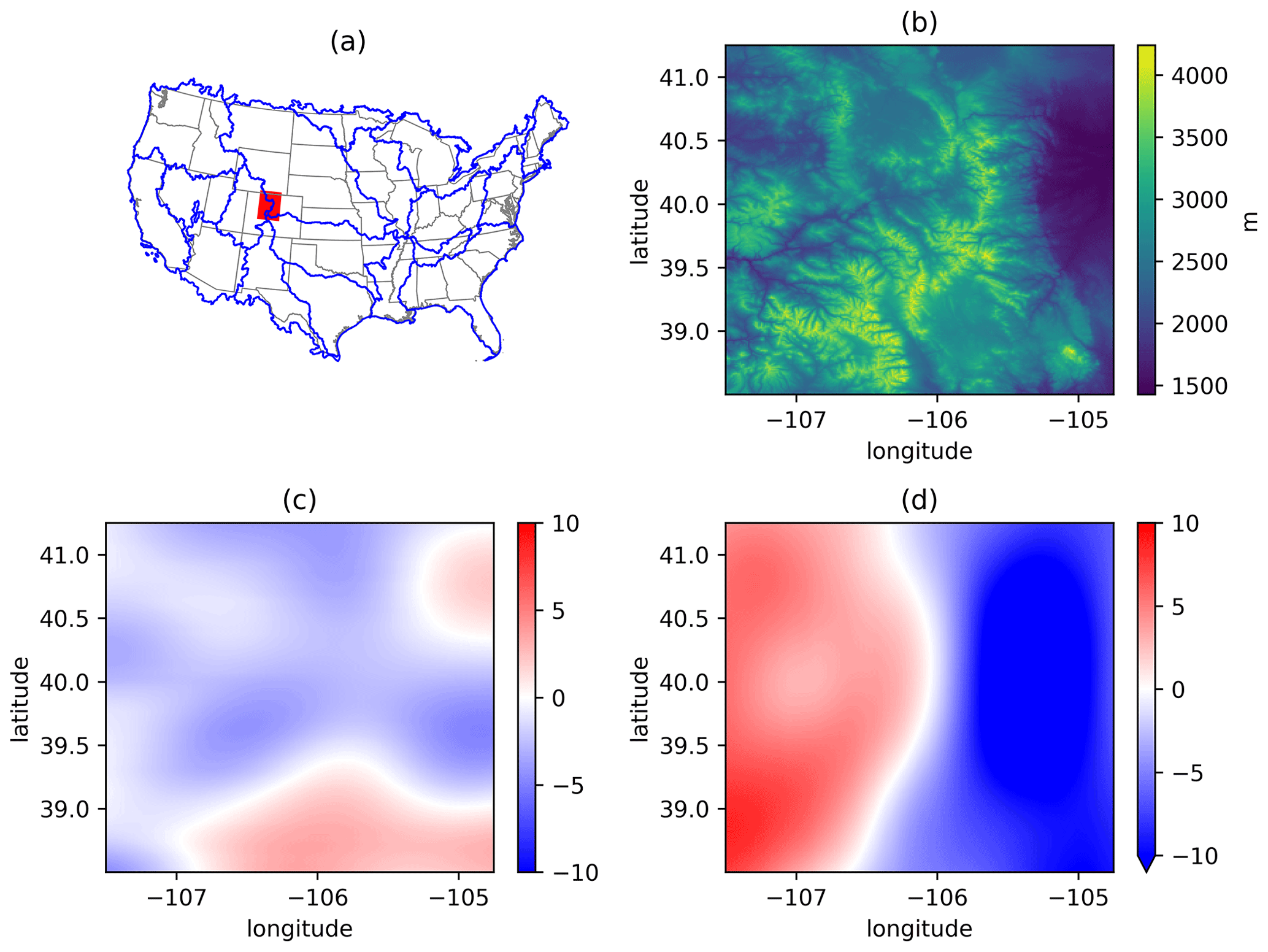
Figure 4 (a) The location of the test case area in the upper Colorado region, USA (red region). Blue lines outline the Hydrologic Unit Code (HUC) level-2 regions. (b) The digital elevation from the Shuttle Radar Topography Mission (SRTM) with an original resolution of 3 arcsec. (c) and (d) are the south–north and west–east slopes, respectively, calculated based on smoothed elevation using a 2D Gaussian low-pass filter.

The high-resolution experiment, having about 73 % of the grid count of the North American Land Data Assimilation System (NLDAS), can also provide a benchmark for large-domain applications. Using 36 CPUs on the Casper high performance computer (HPC) at the National Center for Atmospheric Research, this experiment took 54.4 min to produce regression estimates and 37.3 min to generate 36 ensemble members for the year 2013. Note that this duration does not account for the one-time generation of prior files, such as indices for neighbouring stations and the spatial correlation structure.

4.2.2 Leave-one-out validation

As introduced in Sect. 3, GPEP uses the leave-one-out strategy to estimate the uncertainty of local regression. GPEP also provides 16 evaluation metrics in the output file, facilitating the assessment of the quality of interpolation estimates. For example, Fig. 5 displays three metrics, namely, the correlation coefficients (CC: 0–1), mean absolute error (MAE: 0–∞), and the modified Kling–Gupta efficiency (KGE^′′: −∞–1). KGE^′′ (Tang et al., 2021) uses the standard deviation instead of the mean value to normalize the bias term, making it suitable for temperature variables because it avoids the impact of units (e.g., kelvin vs. degrees Celsius) and the amplified bias around zero temperature (when degrees Celsius is used). Precipitation estimates show higher accuracy in the relatively flat eastern areas, exhibiting high CC and KGE^′′ and low MAE, while the vast western areas have lower accuracy due to the complex terrain and lower station density. Tmean and Trange exhibit different spatial patterns, with Tmean having much better MAE and KGE^′′ than Trange. This indicates the difficulty in capturing diurnal fluctuations between the minimum and maximum temperature.

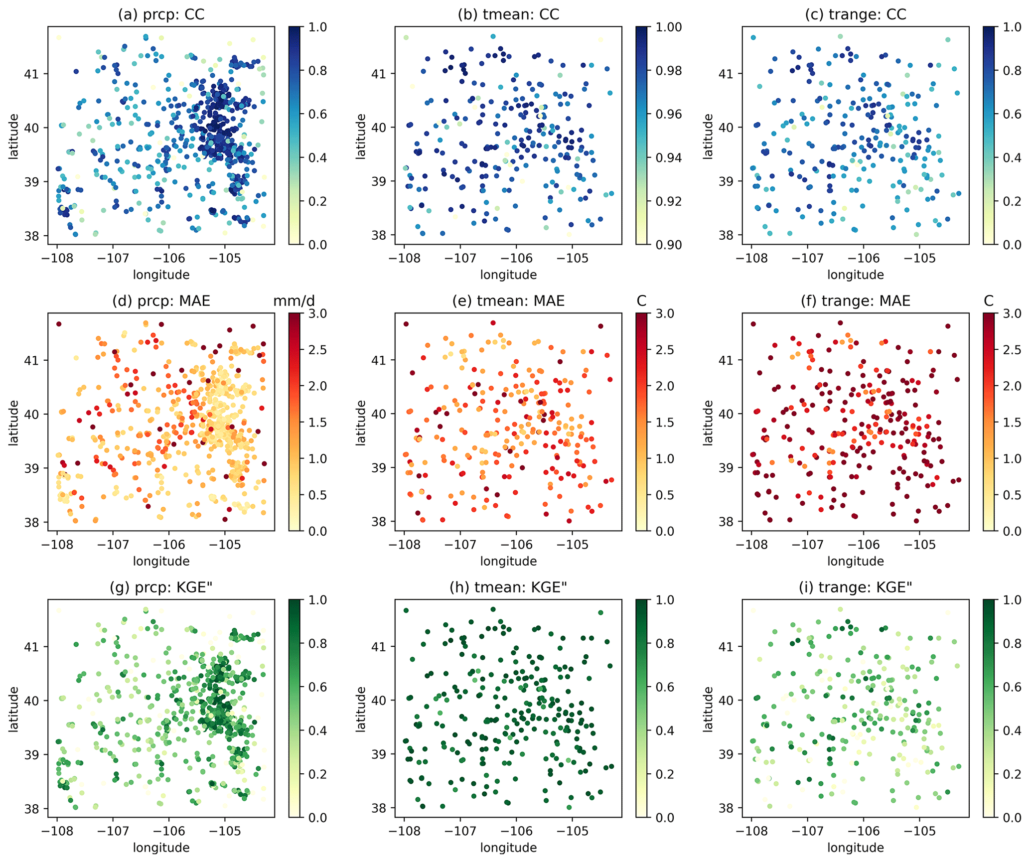
Figure 5 The spatial distributions of CC (a, b, c), MAE (d, e, f), and KGE^′′ (g, h, i) for precipitation (a, d, g), Tmean (b, e, h), and Trange (c, f, i) based on leave-one-out validation.

We compared the performance of RF to locally weighted regression as shown in Fig. 6. Here we only use the default settings of the scikit-learn package. The efficiency of RF is influenced by factors like hyperparameters and feature combinations, but a deep dive into these is beyond the scope of this paper. We used 10-fold cross-validation for RF and leave-one-out for locally weighted regression, making the station density about 10 % lower for RF. Compared to locally weighted regression, RF has better CC for precipitation and Tmean but a higher MAE for all variables. For KGE^′′, the difference between the two methods varies across stations but has a comparable overall performance. This experiment highlights the capability of GPEP to incorporate machine learning in spatial estimation, and refining precision in specific user applications will benefit from the user's expertise.

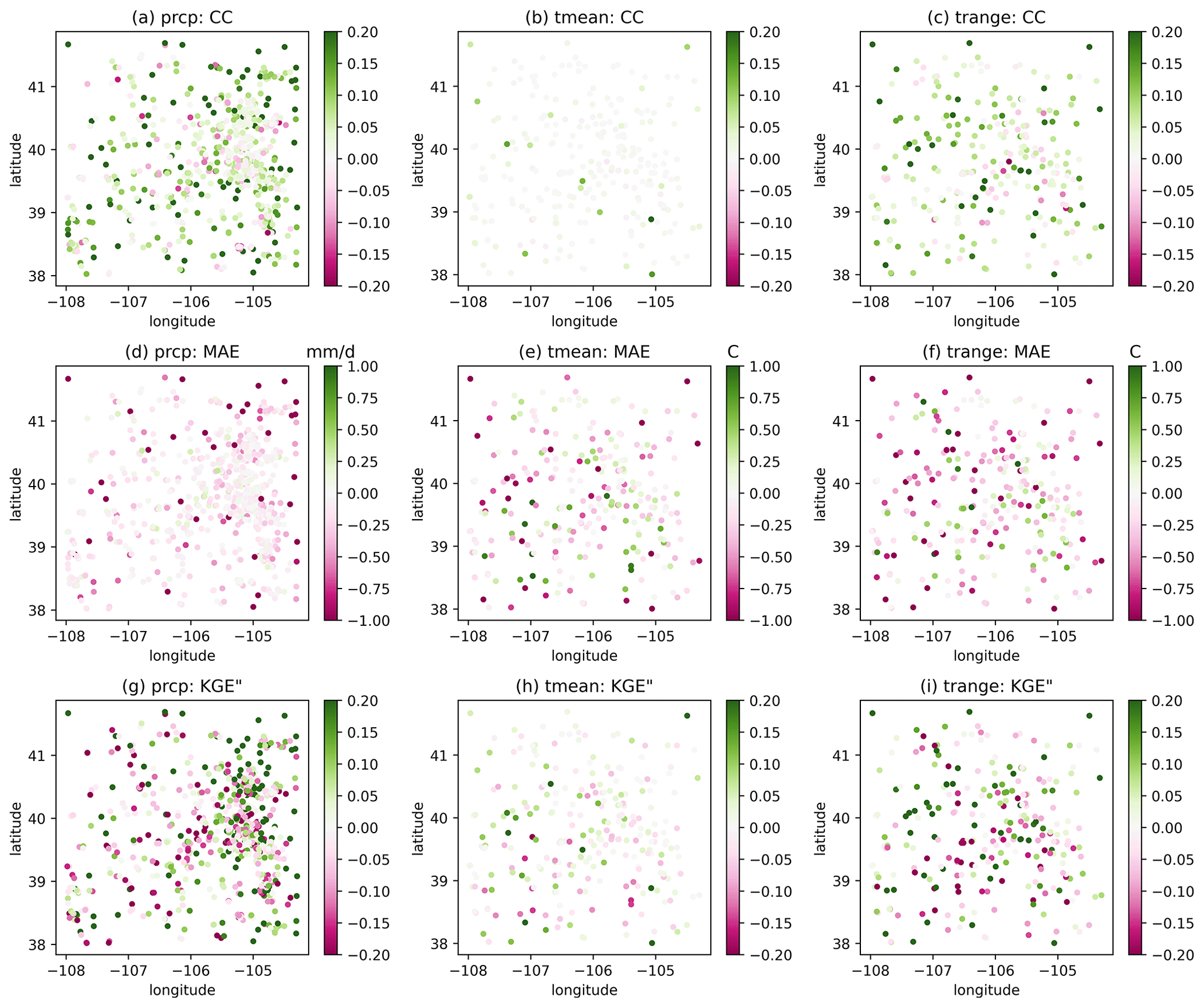
Figure 6 As in Fig. 5 but depicting the difference (random forest minus locally weighted regression) between the two estimation methods. Note that the random forest output is just for demonstration purposes without substantial effort on parameter tuning and feature engineering.

4.2.3 Ensemble estimation

Figure 7 shows the spatial distributions of precipitation, Tmean, and Trange from three ensemble members during the period 9 to 17 September 2013, when heavy precipitation occurred with the accumulated amounts exceeding 500 mm at the precipitation centre. The magnitude is generally comparable to other post-flood analyses (e.g., Gochis et al., 2015). The large differences between members at event centres originate from the interpolation uncertainties which are mainly caused by the degraded capability of the station network and interpolation method to capture extreme events. Tmean shows the lowest ensemble spread among the three variables, and Trange shows the intermediate ensemble spread. The ensemble spread, calculated using weighted spatial averaging, shows a smooth spatial distribution. The distribution of Tmean and Trange demonstrates a distinct patchy pattern, suggesting that the primary source of uncertainty originates from a few stations located in the southern region of the study area.

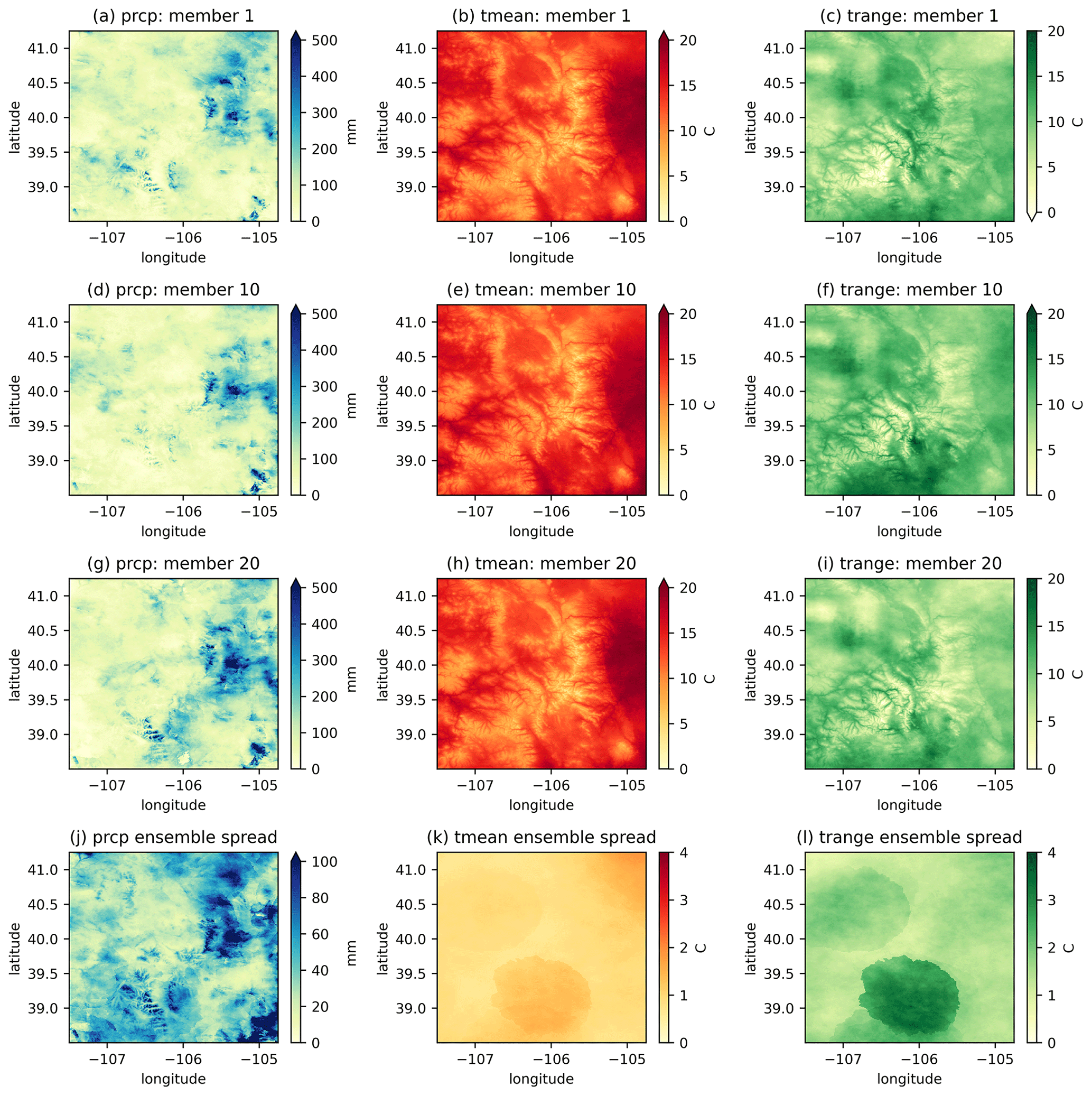
Figure 7 The spatial distribution of total precipitation and mean Tmean/Trange (columns) from three ensemble members (the first three rows) and the ensemble spread (the fourth row) from 9 to 17 September 2013.

Figure 8 shows the time series of ensemble outputs in September 2013 for Boulder County, Colorado, parts of which experienced significant extreme precipitation, causing devastating floods from 11 to 15 September 2013. The return periods of the floods were estimated to be 25 to 100 years. The GPEP ensemble precipitation indicates a major precipitation event (Fig. 8a), with mean or median precipitation going beyond 60 mm d⁻¹ and some members going beyond 100 mm d⁻¹ around 11 September. For precipitation estimation, it is possible that the use of a wind speed and direction dynamic predictor would also contribute to an upslope precipitation enhancement, leading to higher intensities at elevation in the Front Range basins that experienced flooding. The flooding period also suffers from the largest uncertainty in September with the 5 %–95 % bounds ranging between <10 and >150 mm d⁻¹. This illustration highlights the challenge of accurately capturing extreme events with deterministic precipitation estimation and the potential usefulness of ensemble estimation in representing uncertainty and triggering useful alerts for extreme events with their upper bounds. Additionally, Tmean displays a decreasing trend accompanied by continuous precipitation, while Trange shows an inverse trend to Tmean after 8 September.

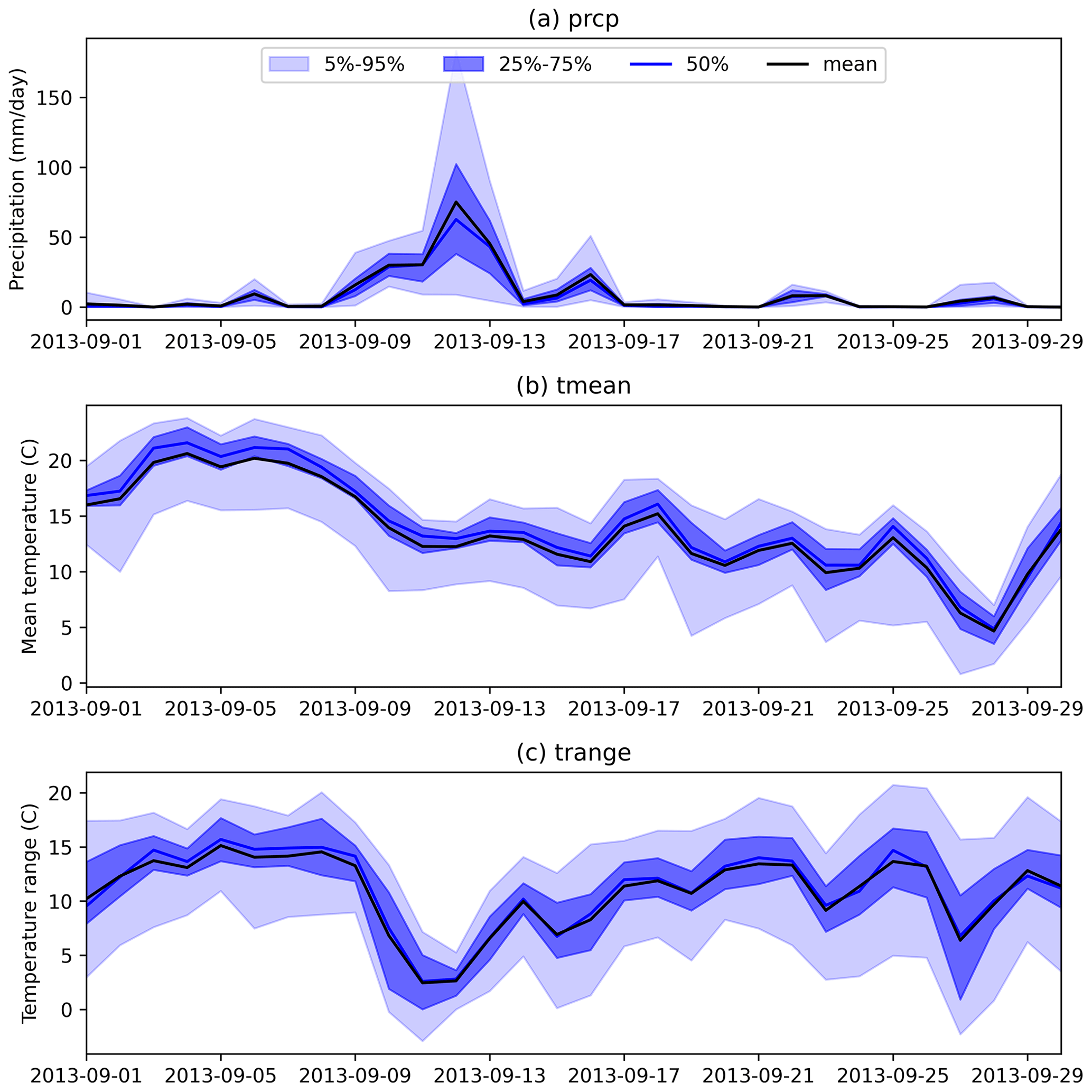
Figure 8 The time series of spatially averaged GPEP ensemble outputs in Boulder County, Colorado (39.91 to 40.26^∘ latitude and −105.7 to −105.05^∘ longitude).

We conducted an additional experiment for an independent evaluation of ensemble estimates. In this experiment, we utilized 70 % of the randomly selected stations to generate the gridded estimates and used the remaining 30 % as a reference for evaluation. The number of ensemble members is 100. As depicted in the rank histogram (Fig. 9), the probabilistic estimates for precipitation, Tmean, and Trange generally capture the range of station observations. Yet, precipitation probabilistic estimates appear to have a slight bias toward overestimation, as shown by the elevated sample number at the lowest rank compared to others, whereas Tmean probabilistic estimates lean toward underestimation. The results depart from uniform reliability across all predicted ranks, though not badly. These biases might stem from inaccuracies in spatial regression estimates and may be improved through a consideration of different predictors or methods available in GPEP. We reiterate that these results serve as a demonstration of the probabilistic evaluation methodology. Users should conduct evaluations tailored to their specific test cases to gauge actual performance.

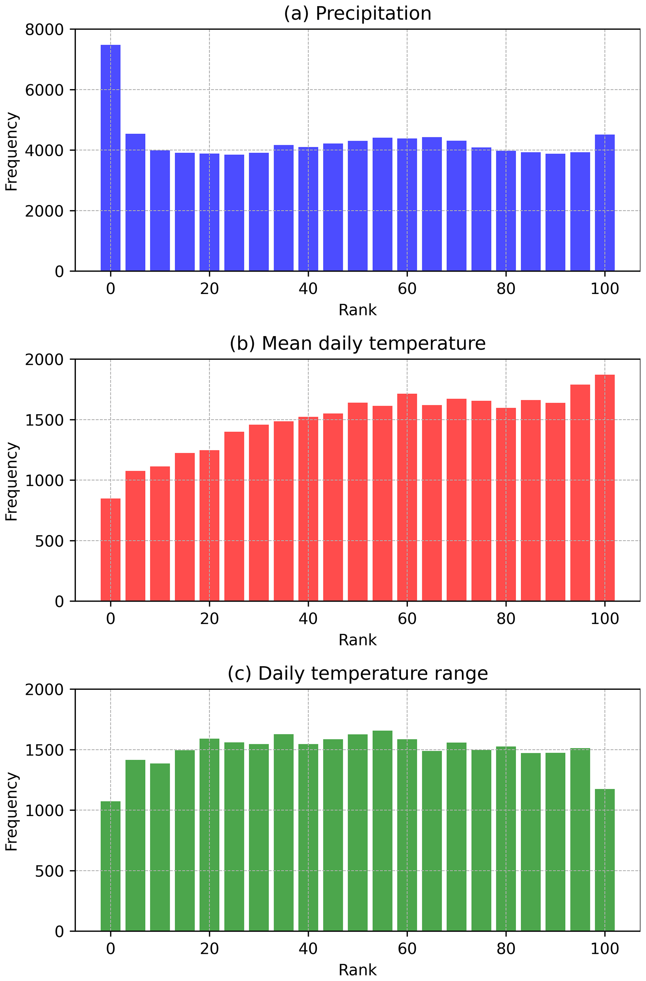
Figure 9 The rank histogram of 100 ensemble members using 70 % of the stations to generate the gridded estimates and the remaining 30 % as the evaluation reference.

4.3 Snow water equivalent (SWE) estimation

GPEP can be applied to a wide range of geophysical variables beyond precipitation and temperature, which has been the common application of GMET. In this test case, snow water equivalent (SWE) is chosen as an example, as it was one of the first applications of the locally weighted terrain regression and ensemble generation methodology that was later developed into GMET (Slater and Clark, 2006). We use the same domain as in the previous test case and a configuration sharing some details: the predictors are latitude, longitude, elevation, and south–north and west–east slopes; the transformation method was Box–Cox; and the locally weighted linear/logistic regression is adopted. In practice, other predictors such as other topographic variables; vegetation types; and dynamic predictors such as radiation, temperature, and SWE from models can be explored for improved performance. We estimate SWE ensembles for the water year from October 2012 to September 2013. The station observations come from the SNOwpack TELemetry Network (SNOTEL). Only serially complete stations (71) in the study period are used, as we did not attempt to quality control and fill the station data for this demonstration.

Figure 10 shows the LOO cross-validation results of SWE. According to station observations, the SWE peak occurs on 25 April 2013, during the 2012–2013 water year. Overall, the spatial distributions of observed and estimated SWE are similar (Fig. 10a and b). However, the estimated SWE is smoother in space, leading to large biases at a few points. For example, SWE is overestimated at two stations (∼39.3^∘ N, 106.6^∘ W and ∼40.2^∘ N, 105.6^∘ W) that show notably lower SWE than surrounding stations. For the mean annual SWE (Fig. 10c), estimates agree well with observations (the relative mean error for the points shown is 2.94 %), except for one outlier corresponding to the station at 40.35^∘ N, 106.38^∘ W. The station has an elevation of 3340 m, where the estimated SWE is 375 mm but the observed SWE is 180 mm. It is possible that the predictors used in this demonstration do not represent the factors affecting SWE distribution well, leading to sub-optimal regression results. Figure 10d shows that the seasonal performance of cross-validated GPEP SWE (averaged across the 71 points) in the upper Colorado region is well captured, except for the underestimation of SWE at the end of the melt period (June 2013). Optimizing this SWE analysis is beyond the purposes of this capability demonstration, and it is likely that different predictor or methodological choices would improve the results shown here.

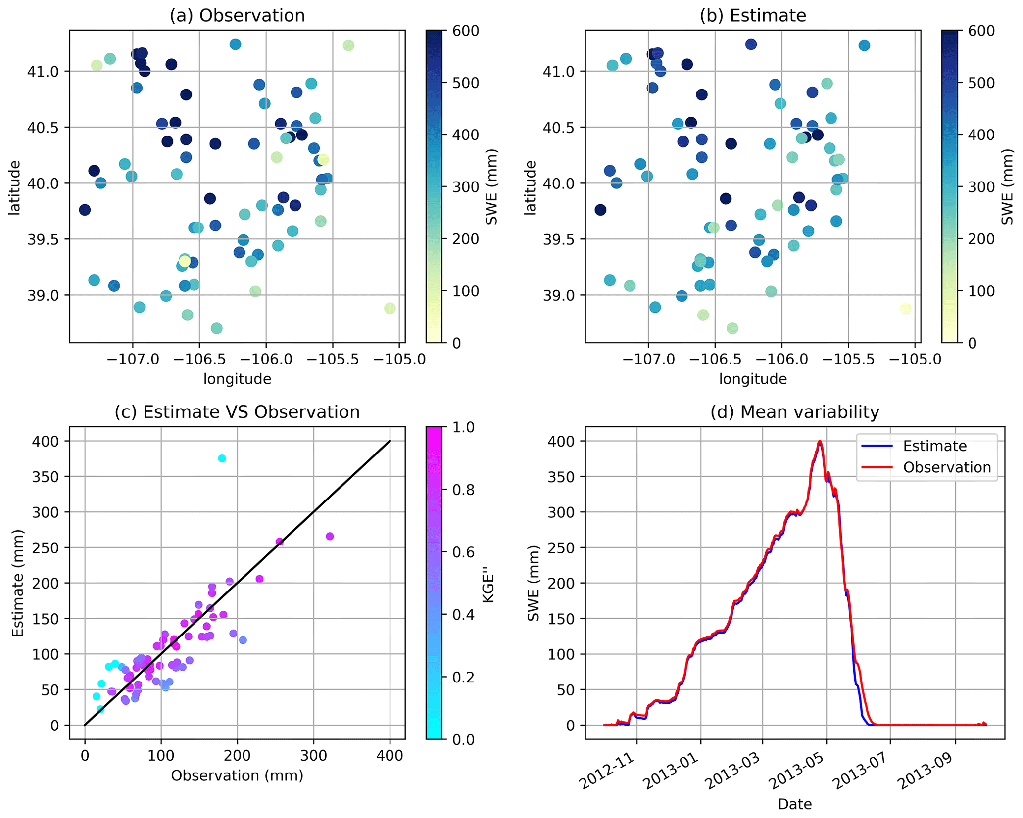
Figure 10 (a) SWE of station observations on 25 April 2013, when the mean SWE reaches the peak, (b) SWE of leave-one-out interpolation estimates on 25 April 2013, (c) scatter plots between observed and estimated mean annual SWE with the colour representing KGE^′′, and (d) the performance of daily domain-average SWE estimation for 1 water year (2013).

SWE and other hydrologic or land surface variables can be strongly auto-correlated, distinguishing their probabilistic estimation from most meteorological fields, e.g., precipitation or temperature. The lag-1 auto-correlation of SWE exceeds 0.99 within the study area, implying that the random field in all time steps will be quite similar to that in the first time step (Eq. 4), and the ensemble spread may be underestimated. This example highlights the importance of generating a realistic initial spatial random field, which significantly depends on the spatial correlation length, for the perturbation of SWE, as well as predictors that represent factors leading to high-frequency space/time variability in SWE. For demonstration purposes, we have used a spatial correlation length of 10 km, but we would encourage future studies to investigate optimal settings for this length. Figure 11 illustrates the 25-member SWE estimates. The uncertainty is lower during the accumulation stage and greater when SWE reaches its peak and melting begins (Fig. 11a). Figure 11b and c display the ensemble mean and spread of SWE on 25 April 2013, respectively. Substantial SWE is observed in high-altitude areas, where the spread is also large. Probabilistic SWE estimates can support the uncertainty quantification of a variety of applications related to water resources management such as forecasting streamflow, including seasonal runoff volumes for managing reservoirs and assessing flood risks.

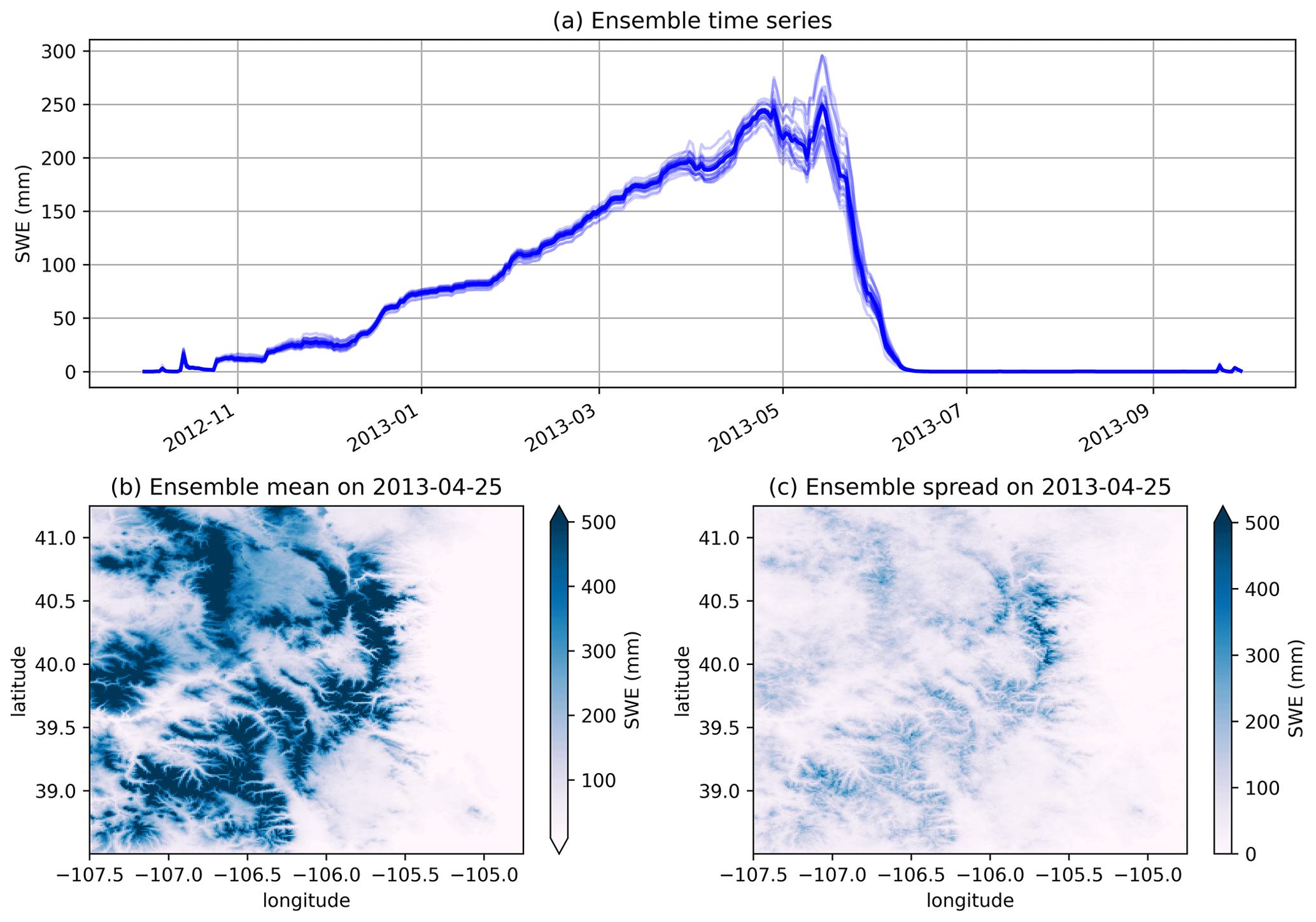
Figure 11 (a) Domain average daily SWE in the study area from 25 members. The dark blue line is the ensemble mean. Panels (b) and (c) are the ensemble mean and ensemble spread of SWE on 25 April 2013, respectively.

5 Discussion

The experiments showcased in this study highlight the flexible use of GPEP for both deterministic and probabilistic geospatial estimation across various variables. We emphasize that GPEP is a tool with a myriad of configuration choices for estimation applications that may differ greatly from the case studies shown. The statistical accuracy of these experiments can be further improved with a deeper dive into predictors, parameters, and methodological alternatives. Users can also investigate the influence of various factors such as station density, topography, and climate on estimation accuracy within their specific applications.

GPEP requires station records as inputs to implement geospatial estimation across temporal scales. For local regression configurations, it is advisable to either fill gaps in station records or utilize serially complete station datasets (e.g., Eischeid et al., 2000; Tang et al., 2020, 2021), while for global regression gaps in station records are permissible. Users also have the flexibility to restructure gridded datasets by considering each grid cell as a distinct station to achieve particular objectives such as downscaling. However, this approach might significantly impact computational efficiency due to the sheer number of points since GPEP is not initially designed to serve such applications.

The initial implementation of GPEP has much room for improvement concerning both methodology and software engineering. A few key aspects are discussed below with the aim to attract a community of collaborators who will help to achieve some of these future developments:

• The probabilistic estimation formulation used by GMET and GPEP is implemented to handle the intercorrelation relationship between two variables, while higher-dimensional multivariate formulations would likely be needed in certain applications of Earth system models. For example, precipitation, humidity, radiation, and temperature variables are correlated to each other in time and space. GPEP only allows the dependencies of one variable on the other one through Eq. (4), although multiple pairs of dependencies can be defined in the configuration file. This formulation can be expanded through code revision to include multivariate correlation and covariance structures, and alternative probabilistic estimation methods can be investigated, such as using Copula functions and reviewing correlation structures obtained from multi-site weather generators.

• The flexibility of the methodological framework can be further enhanced by including more options. For example, myriad options exist for variable transformation (the current Box–Cox transformation may not be ideal) and can be added in the future to address the requirement of specific variables (Papalexiou, 2018). Similarly, the generation of spatiotemporally correlated multivariable analyses can benefit from the addition of a variety of methods, including the Papalexiou and Serinaldi (2020) technique to construct flexible spatiotemporal correlation structures by combining copulas and survival functions, and geostatistical tools such as the Python-based GSTools (Müller et al., 2022) that can be used to generate spatial random fields.

• The current scikit-learn method libraries are just a starting point for expanding the options available for conditional estimation of geophysical fields, and we expect that future development may link to ML and deep learning packages such as PyTorch, TensorFlow, or Keras, as the field evolves. By incorporating these and other potential options, GPEP can become even more versatile in hydrometeorology and Earth science studies.

• A major drawback of the move from the FORTRAN-based GMET to GPEP is the significantly slower outcomes for current meteorological GMET applications (even considering the internal parallel capability of GPEP). Work to understand and optimize this aspect has only begun (e.g., Fig. 2), so the computational demands may pose challenges for GPEP's local regression configurations if applied for large-domain and/or near-real-time operational applications on small computational resources. We expect that this issue can be resolved through further algorithm optimization, hybrid programming for the time-consuming parts of GPEP, additional parallel processing options, and even a shift toward GPU computing.

6 Summary and discussion

GPEP is a flexible Python-based software for ensemble, probabilistic estimation of any geophysical variable. It expands on the capabilities offered by the FORTRAN-based GMET software on which GPEP is based. GMET has been used for almost a decade in numerous hydrology and water resources applications, demonstrating its quality and value through the performance of GMET datasets relative to other widely used options. The central motivations for adapting GMET into a Python framework were to broaden the development community for the probabilistic estimation tool and to facilitate more rapid development with linkages to ML methods through the growing Python-based activities and resources in this area.

GPEP supports various local and global regression methods including ML techniques for spatial interpolation and fusion of multi-sensor datasets, and can generate any number of ensemble members using the predictive uncertainty results obtained from cross-validation. Although GPEP operates more slowly than the original GMET, the tool's internal parallelization capability scales well to improve its computation efficiency, making it suitable for both research and operational applications.

The experiments showcased in this study illustrate examples of GPEP's capabilities without being tailored for optimal application-quality performance. The template configurations available on the associated GitHub repository can emulate GMET configurations and generally deliver commendable results, and users are encouraged to view GPEP as a versatile geospatial estimation tool and extend their configurations beyond those provided in the templates. User expertise and domain knowledge are required for scientific explorations of various configurations (e.g., weight functions, neighbouring stations, static/dynamic predictor combinations, variable transformation, and regression method intercomparison) and diverse scenarios (e.g., station densities, topographic and climatic impacts, and variable choices).