The pseudo-global-warming (PGW) approach: methodology, software package PGW4ERA5 v1.1, validation, and sensitivity analyses

The term “pseudo-global warming” (PGW) refers to a simulation strategy in regional climate modeling. The strategy consists of directly imposing large-scale changes in the climate system on a control regional climate simulation (usually representing current conditions) by modifying the boundary conditions. This differs from the traditional dynamic downscaling technique where output from a global climate model (GCM) is used to drive regional climate models (RCMs). The PGW climate changes are usually derived from a transient global climate model (GCM) simulation. The PGW approach offers several benefits, such as lowering computational requirements, flexibility in the simulation design, and avoiding biases from global climate models. However, implementing a PGW simulation is non-trivial, and care must be taken not to deteriorate the physics of the regional climate model when modifying the boundary conditions. To simplify the preparation of PGW simulations, we present a detailed description of the methodology and provide the companion software PGW4ERA5 facilitating the preparation of PGW simulations. In describing the methodology, particular attention is devoted to the adjustment of the pressure and geopotential fields. Such an adjustment is required when ensuring consistency between thermodynamical (temperature and humidity) changes on the one hand and dynamical changes on the other hand. It is demonstrated that this adjustment is important in the extratropics and highly essential in tropical and subtropical regions. We show that climate projections of PGW simulations prepared using the presented methodology are closely comparable to traditional dynamic downscaling for most climatological variables.

1 Introduction

Climate simulations are an essential tool for studying the expected response of the climate system to greenhouse gas emissions (Flato et al., 2013). Global coupled climate models (GCMs) are used to study the Earth's entire climate system, while regional climate models (RCMs) provide a more detailed description on regional to local scales. These higher-resolution data are crucial for assessing the impact of climate change and for establishing regional mitigation and adaptation strategies (Giorgi et al., 2008; Rummukainen, 2010; Sørland et al., 2020). RCMs are forced by results from GCMs and operate on a finer grid to provide increased detail, a technique that is known as dynamic downscaling (Flato et al., 2013). The standard approach to investigating climate change using RCMs consists of downscaling two time slices from a GCM simulation, one for the future and one for the past, and comparing them or alternatively downscaling a centennial transient simulation (see, e.g., PRUDENCE, Christensen and Christensen, 2007, ENSEMBLES, van der Linden and Mitchell, 2009, and CORDEX, Kotlarski et al., 2014).

While the standard downscaling approach is indispensable for regional climate research, it has several limitations and challenges. For instance, coordinated downscaling efforts require a lot of computing power and data storage. An evaluation run, where the RCM is downscaling a global reanalysis, is required to assess the model performance. Additionally, transient climate simulations are needed to assess the regional climate change. This should be done for multiple RCMs, GCMs, and different emission scenarios to properly represent the full uncertainty range (Hawkins and Sutton, 2009). For several research groups, such applications are beyond the limit of their computational infrastructure (Prein et al., 2015). Another limitation with the traditional downscaling approach is the uncertainty associated with the atmospheric circulation from the GCMs. Even though the RCMs reduce some of the biases from the GCMs (Sørland et al., 2018), the RCMs will not be able to correct for biases in the large-scale circulation from GCMs (Hall, 2014).

1.1 Concept of the PGW approach

In recent years, pseudo-global warming (PGW) simulations have been increasingly used in research as an alternative regional climate modeling strategy. In a PGW simulation, we directly impose selected changes in the climate system on a historical regional climate simulation by modifying the initial and boundary conditions (Schär et al., 1996; Wu and Lynch, 2000; Sato et al., 2007; Rasmussen et al., 2011; Liu et al., 2017; Adachi and Tomita, 2020). In simple mathematical terms, the pseudo-global warming concept can be expressed as

$$\begin{array}{}\text{(1)}& \mathrm{PGW}=\mathrm{CTRL}+\mathrm{\Delta },\end{array}$$

where CTRL and PGW represent the boundary conditions of two RCM simulations of the past and future climates, respectively, and Δ is the future changes often referred to as climate change deltas. Δ must be computed from a separate climate projection as

$$\begin{array}{}\text{(2)}& \mathrm{\Delta }=\mathrm{SCEN}-\mathrm{HIST},\end{array}$$

where SCEN is a future time slice of a climate projection and HIST is the corresponding historical time slice coming from a GCM or RCM simulation. Both SCEN and HIST periods must be chosen to be long enough to reduce the effects of internal variability (average of ∼ 30 years). While the general concept as shown by Eq. (1) is common to most PGW simulations in the literature, the design of both Δ and CTRL varies. In Sect. 2, we will describe in detail how Δ can be derived in practice. We also provide software written in Python to perform this task. Generally, Δ has to be made up of changes in temperature, humidity, wind, and pressure/geopotential. Thereby it is essential to maintain the physical balances in the perturbed boundary conditions of the PGW simulation, in particular the hydrostatic balance. Violations of the hydrostatic balance may occur due to the implied temperature changes but also due to differences in the vertical coordinate and topography between the driving GCM and the RCM boundary conditions. After applying Δ to the thermodynamic variables, it is thus essential to restore this balance using an adequate pressure adjustment (see Sect. 2). Figure 1 shows an example of a PGW-driven RCM simulation along with the corresponding CTRL simulation.

At first glance it is surprising that one can change the driving fields of an RCM simulation in an ad hoc fashion as depicted above without introducing serious inconsistencies in the atmospheric dynamics. Indeed, changes in temperature T will imply changes in pressure and horizontal pressure gradients, thereby affecting the hydrostatic and geostrophic balance of the atmospheric flow. If such changes are enforced inconsistently, the atmosphere will respond with a geostrophic adjustment process. Such an adjustment is potentially important, and indeed it was the root cause behind the failure of the first numerical weather prediction forecast of Lewis F. Richardson (Lynch, 2006). However, the PGW approach rests on a solid theoretical foundation. If ΔT_v is only a function of pressure, i.e., if ΔT_v=ΔT_v(p), where T_v denotes the virtual temperature, the prescribed thermal modification does not modify the horizontal gradient of the geopotential on pressure surfaces, and hence there is no change to the dynamical forcing (Schär et al., 1996). In essence, the balance of forces is unchanged, irrespective of a temperature change ΔT_v(p). When considering the more general case of baroclinic temperature changes, i.e., when $\mathrm{\Delta }{T}_{\mathrm{v}}=\mathrm{\Delta }{T}_{\mathrm{v}}(x,y,p)$, the situation becomes more complex and a simple theoretical argument does not appear to exist. However, a number of numerical studies have demonstrated that undesirable inconsistencies do not occur or are negligibly small. Early studies of this type include those of Kimura and Kitoh (2006) and Sato et al. (2007).

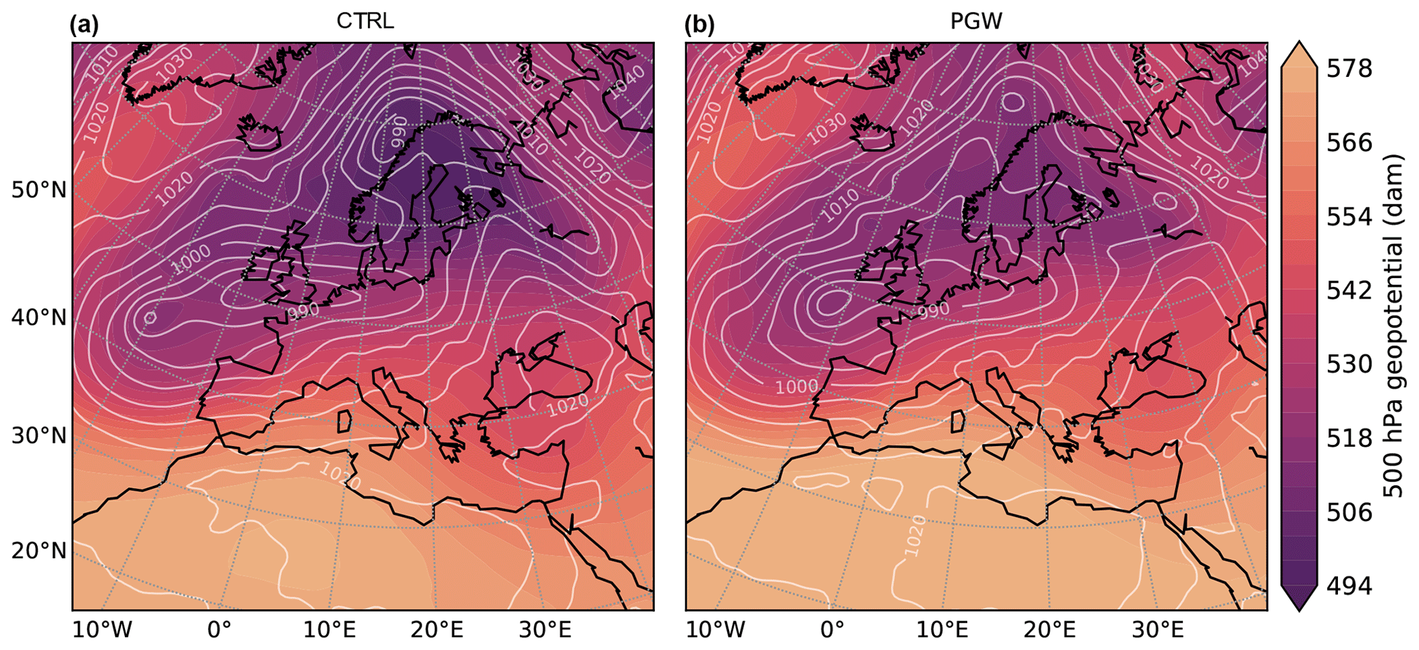
Figure 1 Snapshot of 500 hPa geopotential and mean sea level pressure in a CTRL and PGW-driven simulation representing past and future conditions, respectively. Shading shows the geopotential as indicated by the color bar. White contours show mean sea level pressure (hPa). (a) Evaluation run driven by the ERA-Interim reanalysis. (b) PGW simulation of the same time step. The time of the evaluation run is 30 December 2009 at 00:00 UTC. More details on the model setup can be found in Table A1. Note how the lateral boundary forcing serves to approximately maintain the circulation in the lateral boundary zone, while the system evolves freely in the interior of the domain. Also, the geopotential is generally higher in the PGW simulation shown in panel (b) because of higher atmospheric temperatures.

1.2 Advantages and disadvantages of PGW simulations

Why and when could a PGW simulation be useful? We summarize potential advantages and disadvantages below.

1. The PGW approach makes climate projections with a comparatively short simulation duration possible. Δ is designed to have a seasonal cycle but no interannual variability. Thus, the same Δ is used to modify the boundary conditions of each simulated year. Therefore, there is no change in interannual variability in the future projection. As a result, a period shorter than the typically used 30 years suffices to assess climate change (Yoshikane et al., 2012). This is especially attractive for producing computationally demanding high-resolution climate projections (Schär et al., 2020).

2. PGW simulations can also reduce the computational and storage costs of climate projections if a reanalysis-driven evaluation simulation is pre-existing. Using the PGW approach, this simulation can be modified, and thus only one additional simulation is necessary to assess climate change (no need to dynamically downscale past and future periods from a GCM). The PGW approach is thus attractive when considering a multi-model ensemble of high-resolution simulations (e.g., Pichelli et al., 2021).

3. For the CTRL period, PGW simulations “inherit” the synoptic environment and weather situation from the reanalysis at the lateral boundaries. Thus, the frequency of weather systems entering the domain and the large-scale synoptic situation in the PGW simulation closely matches the reanalysis (Fig. 1). On the one hand, this greatly reduces biases during the CTRL period in comparison to conventional downscaling (where the RCM inherits biases from the driving GCM CTRL). Biases during CTRL are a considerable challenge in impact assessment. For instance, a temperature bias of a few degrees implies biases in the snow line of several hundred meters. The PGW methodology also allows for directly assessing what an observed historical event could look like in a different climate. This approach has recently been recommended as the “storyline” approach to vulnerability assessment (Hazeleger et al., 2015; Shepherd, 2019). On the other hand, using the same synoptic forcing in both CTRL and PGW implies that potential changes in intra-annual and interannual variability might be missed in the PGW approach.

4. To calculate $\mathrm{\Delta }=\mathrm{SCEN}-\mathrm{HIST}$, only data from a few variables of the driving climate projection are needed. This means that the full GCM data do not need to be downloaded and preprocessed to run a RCM simulation. Δ can even be derived from monthly mean data.

5. Δ cannot only represent input from a single GCM or RCM, but an ensemble mean of a set of simulations can also be used to drive a PGW simulation.

PGW simulations are not a standard approach included in regional climate model codes. Thus, preparing PGW simulations needs manual work to produce the initial and lateral boundary conditions. With the software described here, we try to simplify this process.

1.3 Applications

A common application of PGW simulations in research is to investigate a question of the type “How will certain historical or observed events change in a different climate?” Such events can be tropical cyclones (Lynn et al., 2009; Ito et al., 2016; Sørland and Sorteberg, 2016; Gutmann et al., 2018; Patricola and Wehner, 2018; Jung and Lackmann, 2019), mesoscale convective systems (Prein et al., 2017; Haberlie and Ashley, 2019), atmospheric rivers (Dominguez et al., 2018), droughts (Seneviratne et al., 2002; Ullrich et al., 2018), or similar phenomena.

Since they allow for computationally cheap climate projections, PGW simulations can be used to replace standard downscaling, for example, to investigate changes in precipitation (Sato et al., 2007; Kawase et al., 2009; Taniguchi, 2016; Dai et al., 2020; Rasmussen and Liu, 2017; Wang and Wang, 2019), local temperature (Adachi et al., 2012; Expósito et al., 2015), clouds (Hentgen et al., 2019), or snow cover (Hara et al., 2008; Kawase et al., 2013; Ikeda et al., 2021).

Applications beyond the two mentioned above have also been explored. PGW simulations can be used to quantify the role of different drivers of climate change (Rowell and Jones, 2006; Kendon et al., 2010; Kröner et al., 2017; Keller et al., 2018; Brogli et al., 2019a, b).

The PGW approach can also be used to debias a GCM simulation when using it for conventional downscaling with an RCM (similarly to Misra and Kanamitsu, 2004). In this case, one has to use some reanalysis ERA and define the climatological mean Δ as $\mathrm{\Delta }=\mathrm{ERA}-\mathrm{HIST}$ representing the GCM bias. The debiased control simulation is then driven by $\mathrm{CTRL}=\mathrm{HIST}+\mathrm{\Delta }$ (HIST here represents the GCM output at full temporal resolution) and similarly for the scenario simulation. This removes the mean bias of the driving GCM simulation.

1.4 Goal and outline

With this article, we aim to facilitate the future generation of reanalysis-driven PGW simulations by providing the software PGW4ERA5 (Pseudo-Global Warming for ERA5) designed for this purpose along with the article. In Sect. 2 we describe in detail the methodology used in the software package. In Sect. 3, we will present the properties of PGW simulations prepared with our methodology. Even though the PGW approach is often used, such studies on the general simulation properties are sparse (e.g., Yoshikane et al., 2012). Before concluding, we present multiple sensitivity tests regarding the design of PGW simulations in Sect. 4. We omit an extensive review of the literature on the subject as this can be found in Adachi and Tomita (2020).

2 Methodology and software

In this section we describe in detail the PGW methodology and its implementation in our Python software PGW4ERA5. We have performed multiple tests to arrive at the described strategy, many of which will be presented in Sect. 4.

2.1 Reanalysis data

The PGW4ERA5 software is designed to facilitate the derivation of the PGW boundary conditions for a reanalysis-driven CTRL simulation. In principle, the concepts are applicable for any kind of reanalysis, but PGW4ERA5 is designed for the use of the European Centre for Medium-Range Weather Forecasts (ECMWF) ERA5 reanalysis (Hersbach et al., 2020). The standard ERA5 reanalysis output is given on a hybrid sigma-pressure coordinate. While output on pressure levels is also available and can be used to drive RCM simulations, we focus here on the use of ERA5 data on the native hybrid coordinate. Using ERA5 data on the native vertical coordinate has the advantage that the full vertical resolution is used. This is for instance essential in cases with pronounced inversions. Extending the code to the use of ERA5 data on pressure levels may be subject to future code developments and would require updating the pressure adjustment (see Sect. 2.8).

2.2 GCM data

The climate deltas used in the PGW approach should represent differences between two climatological periods. In practice we take the differences of two extended periods (e.g., 30 years) from a transient scenario simulation, representing, for instance, the changes between the recent climate and the end of the century for some greenhouse and aerosol emission scenario. We have been working with three different sources of CMIP GCM data obtained from the Earth System Grid Federation download portal (Cinquini et al., 2014).

1. Complete GCM output. Daily or subdaily three-dimensional data provided on the original GCM grid in terrain-following coordinates. Such data are only available for some GCMs and usually not globally but only over certain domains. The CMIP6 output group CFday is one example of such data that are available for a small number of models.

2. AMON data. Average monthly mean data on 19 pressure levels available from virtually all CMIP simulations. Experience with these data suggests that the vertical resolution is sufficient for applications in the extratropics.

3. EMON data. For a selection of models, a similar data set exists with a higher vertical resolution with 27 pressure levels. In simulations where strong inversions are present (e.g., over the tropical and subtropical oceans), the higher resolution of the EMON data should be beneficial.

While in this paper we show some examples using full GCM output data, the presentation of the procedure does focus on the case where we use pressure-level GCM data. The GCM data used to construct the climate change signal are listed in Table 1. This includes the usual atmospheric three-dimensional fields. As to be demonstrated later (see Sect. 4.3), it is advantageous to use relative humidity (RH) rather than q_v; if only the latter is available, q_v is converted into RH. There are alternative approaches to treat the humidity change, such as the assumption of no change in RH with warming (e.g., Adachi and Tomita, 2020). Such modifications are straightforward to implement through the modification of ΔRH. We note that caution is required for temperatures below 0 ^∘C, where the definition of RH may differ between models. Our software uses the definition of saturation vapor pressure over water and ice following the implementation in the Integrated Forecasting System (IFS) model.

Table 1 Data requirements: pressure-level monthly-mean data from the driving GCM.

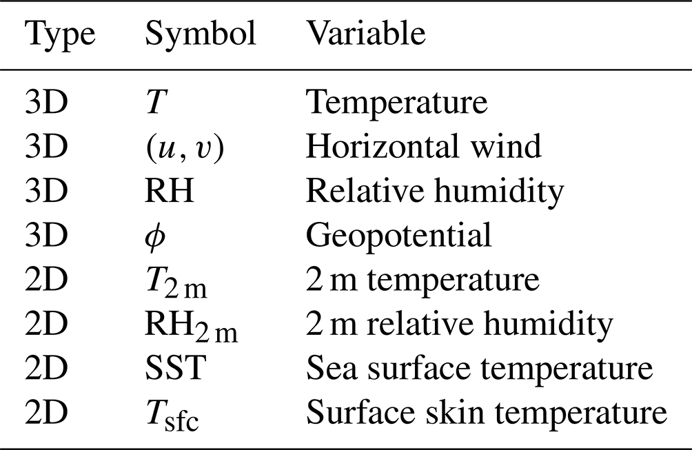
The geopotential ϕ is also available as a three-dimensional field. However, in the simplest case we only require one level, i.e., ϕ_ref at reference pressure level p_ref. This information is sufficient to reconstruct the three-dimensional geopotential field using the hydrostatic equation. The pressure level p_ref must be chosen to be located above the surface throughout the geographical domain considered. In cases with high topography, one may also use different reference pressure levels in different areas of the domain (see Sect. 2.9.2).

The procedure uses 2 mm data for RH_2 m and T_2 m to improve the vertical interpolation of T and RH near the surface. The surface and soil temperature change is derived using T_sfc and sea surface temperature (SST) (see Sect. 2.7). Soil moisture data are not used as different models' soil moisture has different meanings. Initial soil moisture for the RCM simulation must thus be reconstructed by a simulation over an extended spinup period.

The climate change delta for each of the variables χ listed above is computed on the GCM mesh as

$$\begin{array}{}\text{(3)}& \mathrm{\Delta }\mathit{\chi }={\mathit{\chi }}_{\mathrm{SCEN}}-{\mathit{\chi }}_{\mathrm{HIST}}.\end{array}$$

The SCEN−HIST differences represent averages of two climatological periods (e.g., 30 years each), either at monthly (January–December) or daily resolution. In PGW4ERA5, the climate deltas are stored and processed in netCDF format (https://doi.org/10.5065/D6H70CW6, Rew and Davis, 1990). The handling of the netCDF files is done with the xarray Python package (Hoyer and Hamman, 2017).

2.3 Overview of the workflow

The PGW4ERA5 software package uses as input the underlying GCM simulation(s) and the reanalysis (abbreviated as ERA in the following). The package outputs the PGW-modulated reanalysis. The overall workflow of PGW simulations is shown in Fig. 2. The figure uses the convention that the subscripts denote the respective computational mesh (see caption). The RCM simulation under past or current climate conditions (CTRL_RCM) follows the usual procedure of an ERA-driven RCM simulation: ERA is interpolated to the RCM grid with a temporal resolution of a few hours and then drives the RCM simulation at the lateral and lower boundaries. The interpolation step is highly dependent on the domain and type of vertical coordinate of the target RCM. Here we assume that such an interpolation module exists with the RCM considered. In the case of the COSMO-CLM model (Rockel et al., 2008; Sørland et al., 2021), the procedure is able to handle two height-based terrain-following hybrid coordinates (Schär et al., 2002; Baldauf et al., 2011). Boundary and initial condition files typically contain many more variables than those modified by the PGW approach. These variables (e.g., soil type, liquid and solid water species, aerosol concentrations) are left to the interpolation procedure of the RCM, which anyway must be able to provide some information at the lateral boundaries, irrespective of whether this information is provided by the driving model or not. For instance, the concentrations of condensed water species are often not available, and if present, one needs to keep in mind that they strongly depend on the microphysics scheme used.

For the PGW simulation, the ERA fields are modified by the climate change deltas Δ. This step requires the interpolation of the respective fields from the GCM to the ERA computational mesh. The procedure is complicated because of the pressure adjustment that is required (see below).

Alternatively, one could add the deltas directly to the CTRL_LBC. However, it is more consistent to add these to CTRL_ERA in order to ensure that the same interpolation procedures are used for both RCM simulations. Note in particular that the interpolation procedures commonly used to generate the lateral and lower boundary conditions of RCM simulations are complex and far beyond a pure interpolation. For instance, they may invoke nonlinear heuristic procedures to account for differences in topographical height. In addition, as all RCMs are equipped to use reanalyses, the ERA file format is a useful interface between our PGW code and the RCM model.

Greenhouse gas (GHG) concentrations can be raised in the PGW simulation, consistent with those imposed in the GCM. In practice, this procedure depends on the RCM considered. It is important to note, however, that the prime effects of changes in GHG concentrations happen in the GCM, where they drive the large-scale warming and moistening. This signal reaches the RCM via the lateral boundaries, and this is more important than local radiative effects in the RCM (e.g., Seneviratne et al., 2002). Nevertheless, we recommend adjusting the forcing consistent with the driving GCM, also as the CO₂ concentration may affect evapotranspiration, depending on the land surface model considered (e.g., Schwingshackl et al., 2019). The situation is similar regarding changes in aerosol concentrations. While representing changes in regional aerosol concentrations is important (e.g., Boé et al., 2020), we are not aware of PGW simulations that fully represent this effect.

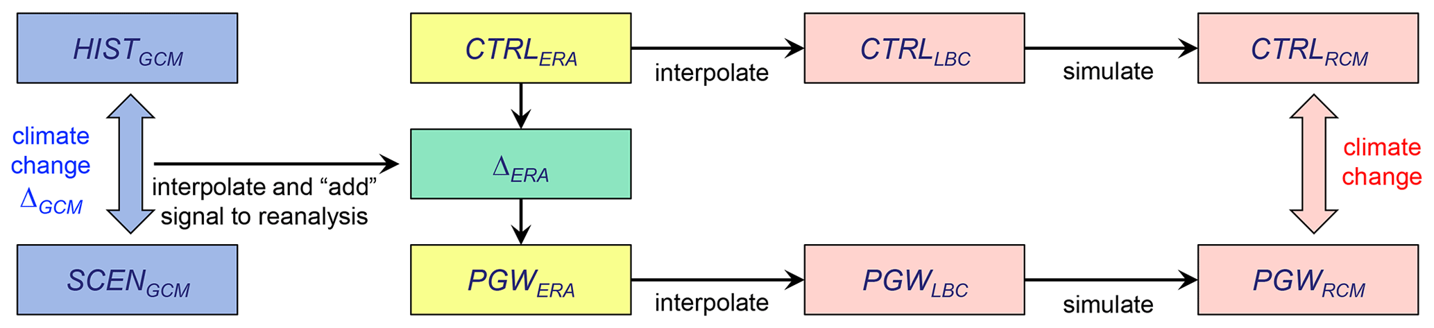
Figure 2 Workflow for PGW simulations. The strategy consists of imposing large-scale changes in thermodynamic structure and circulation on a historical RCM simulation by modifying the lateral and lower boundary conditions correspondingly. The climate change signal is taken from GCM simulations. Here CTRL and PGW represent the historical and pseudo-global-warming simulations, driven by historical and modulated reanalysis, respectively. The subscripts denote the underlying computational mesh, represented by the GCM, the reanalysis ERA, the regional climate model RCM, and the lateral and lower boundary conditions LBC driving the RCM. Note that the LBC and RCM meshes are typically identical.

2.4 Reconstruction of the CTRL ERA geopotential

The standard ERA5 reanalysis files contain all relevant three-dimensional fields but neither the pressure nor the geopotential height field. Rather, the surface pressure p_sfc is provided. It determines the pressure of all computational levels through the definition of the hybrid vertical coordinate as

$$\begin{array}{}\text{(4)}& p_{k+\mathrm{1}/\mathrm{2}}=a_{k+\mathrm{1}/\mathrm{2}}+p_{\text{sfc}}{b}_{k+\mathrm{1}/\mathrm{2}}.\end{array}$$

Here, subscripts k and $k+\mathrm{1}/\mathrm{2}$ denote the layer centers and interfaces, respectively (numbered from top to bottom), and the coefficients a and b define the hybrid coordinate. As p_sfc denotes the surface pressure at the height of the ERA topography, it cannot directly be merged with the Δp_sfc from the GCM, as the latter is located at a different height. To resolve this problem, Δϕ at the GCM pressure level p_ref is used instead. In the simplest case, one chooses one single pressure level p_ref located above the topography for the whole RCM domain.

The reconstruction of the geopotential on the computational mesh of the ERA reanalysis uses the hydrostatic equation in pressure coordinates

$$\begin{array}{}\text{(5)}& {\displaystyle \frac{\partial \mathit{\varphi }}{\partial p}}=-{\displaystyle \frac{R{T}_{\mathrm{v}}}{p}}.\end{array}$$

In numerical terms, this means integrating from the surface ($k=K+\mathrm{1}/\mathrm{2}$) to the top using

$$\begin{array}{}\text{(6)}& \begin{array}{rl}{\mathit{\varphi }}_{k-\mathrm{1}/\mathrm{2}}& ={\mathit{\varphi }}_{k+\mathrm{1}/\mathrm{2}}-(\ln p_{k-\mathrm{1}/\mathrm{2}}-\ln p_{k+\mathrm{1}/\mathrm{2}})R{T}_{v,k}\\ & \mathrm{for}k=K,K-\mathrm{1},\mathrm{\dots },\end{array}\end{array}$$

with the lower boundary condition ${\mathit{\varphi }}_{K+\mathrm{1}/\mathrm{2}}={\mathit{\varphi }}_{\text{sfc}}$. Here $T_{\mathrm{v}}=f(T,q_{\mathrm{v}})$ or $T_{\mathrm{v}}=f(T,\mathrm{RH},p)$ is known from the definition of the virtual temperature. The geopotential at the reference level, i.e., ϕ_ref=ϕ(p_ref), is derived using linear interpolation in ln (p). This yields

$$\begin{array}{}\text{(7)}& {\mathit{\varphi }}_{\mathrm{ref}}={\mathit{\varphi }}_{k^{*}+\mathrm{1}/\mathrm{2}}-(\ln p_{\mathrm{ref}}-\ln p_{k^{*}+\mathrm{1}/\mathrm{2}})R{T}_{v,k^{*}},\end{array}$$

where $k^{*}+\mathrm{1}/\mathrm{2}$ is the grid point immediately below the p_ref level, i.e., $p_{k^{*}+\mathrm{1}/\mathrm{2}}\ge p_{\mathrm{ref}}\ge p_{k^{*}-\mathrm{1}/\mathrm{2}}$. The reference geopotential ϕ_ref(x,y) will later be combined with the respective changes Δϕ_ref(x,y) from the GCM simulation.

2.5 Interpolation of PGW changes in time

Regional climate models operate with a specified boundary update frequency of typically 1 to 6 h. To run a PGW simulation, we require the Δ signal at the same frequency, accounting for the mean seasonal cycle of the signal. We apply two different methodologies. First, if the computations are based on monthly mean data, the continuous function is computed by linear interpolation (Fig. 3, orange line). Second, when using input with daily frequency, the 30-year mean annual cycle (Fig. 3, green line) is subjected to the spectral filtering algorithm described in Bosshard et al. (2011), which returns a smoothed annual cycle with daily frequency (Fig. 3, blue line). Linear interpolation is subsequently used between the daily values to obtain a continuous function for the annual cycle of Δ at the boundary update frequency of the RCM.

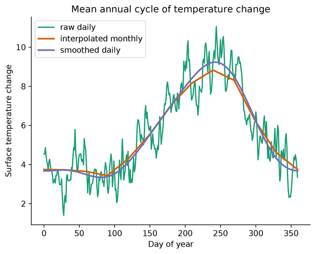
Figure 3 Mean annual cycle of the PGW climate change signal at a specific grid point in Europe for different methods of constructing the annual cycle from GCM data. The green line shows the raw signal from two 30-year periods at daily resolution. It is strongly influenced by daily and interannual variability. The orange and blue lines show different methods of constructing a smooth and continuous annual cycle. The orange line shows the result of linear interpolation between monthly mean values. The blue line is the result of smoothing the daily values using spectral filtering. Both filtering methods are supported by PGW4ERA5.

2.6 Application of PGW changes to ERA fields

For each datum in the lateral boundary forcing fields, we add the Δ_GCM to the ERA reanalysis (see Fig. 2). To this end, Δ needs to be spatially interpolated from the GCM to the ERA grid, i.e., Δ_ERA. In the horizontal, the changes are bilinearly interpolated. For complicated geographical coordinate systems of the input data set, the xESMF Python package is available (Zhuang et al., 2020). For the three-dimensional variables ΔT, Δu, Δv, and ΔRH, we also require an interpolation in the vertical from the GCM pressure levels to the ERA hybrid levels, which again uses linear interpolation in ln p. Ultimately, for three-dimensional ERA fields χ, Δ is applied as

$$\begin{array}{}\text{(8)}& \begin{array}{rl}{\mathit{\chi }}^{\prime }(x,y,p)& =\mathit{\chi }(x,y,p)+\mathrm{\Delta }(x,y,p)\\ & \mathrm{for}\mathit{\chi }=T,u,v,\mathrm{RH}.\end{array}\end{array}$$

Here χ and χ^′ denote the ERA and PGW variables, respectively.

The pressure values for the ERA hybrid vertical levels depend on the surface pressure p_sfc. When doing the vertical interpolation, we make the assumption that the surface pressure does not change, i.e., $p{}_{\text{sfc}}^{\prime }\approx p_{\text{sfc}}$. This is an approximation, but tests demonstrated that relaxing this assumption leads only to minimal changes (see Sect. 2.9.1).

The application of Eq. (8) to the two-dimensional surface fields is straightforward. Similarly, the Δ is also imposed to the geopotential at the reference pressure level p_ref as

$$\begin{array}{}\text{(9)}& \mathit{\varphi }{}_{\mathrm{ref}}^{\prime }:={\mathit{\varphi }}_{\mathrm{ref}}+\mathrm{\Delta }{\mathit{\varphi }}_{\mathrm{ref}},\end{array}$$

where ϕ_ref is defined by Eq. (7).

2.7 Surface fields

Over land, the temperature change in the soil levels is derived based on ΔT_sfc following

$$\begin{array}{}\text{(10)}& \mathrm{\Delta }T\left(z\right)=\stackrel{\mathrm{‾}}{\mathrm{\Delta }{T}_{\text{sfc}}}+e^{z/\mathrm{2.8}\mathrm{m}}(\mathrm{\Delta }{T}_{\text{sfc}}-\stackrel{\mathrm{‾}}{\mathrm{\Delta }{T}_{\text{sfc}}}),\end{array}$$

where ΔT(z) is the soil temperature change at depth z (m) and $\stackrel{\mathrm{‾}}{\mathrm{\Delta }{T}_{\text{sfc}}}$ is the annual mean of ΔT_sfc (i.e., representing the climatological deep soil temperature change). The constant 2.8 m is the penetration depth of the annual cycle for an average thermal conductivity of the soil. A similar procedure is applied when interpolating the driving fields to the mesh of the COSMO models.

Over sea, RCMs typically use prescribed sea surface temperature, which is modified here based on ΔSST. The difficult aspect is that ΔSST is defined on the ocean model grid of the GCM, which typically has a complex grid geometry and is undefined over land. The interpolation of ΔSST to the ERA grid thus requires special attention. The problem is illustrated in Fig. 4. Using naive bilinear interpolation, the missing values (NaN) from land regions are propagated into the ocean ΔSST field, and coastlines are missed (Fig. 4b). A more sophisticated interpolation routine is used instead, which ignores the contribution from NaN values. This is done by removing all grid points of the GCM grid over land and re-casting it to an unstructured grid. A Gaussian kernel-based interpolation method (Maz'yai and Schmidt, 1996) is used to interpolate the ΔSST field onto the ERA ocean grid points. With this approach, a ΔSST value can be obtained for all water grid points in the ERA data set, and no information is lost at the coastlines (Fig. 4c). A user-defined kernel cutoff value (i.e., the maximum distance across which ΔSST values are interpolated) can be set to avoid water basins lacking GCM information getting a far-lying ΔSST value from a remote ocean basin. Instead, for these cases, the method falls back to the ΔT_sfc to derive the local water surface temperature change. However, as the method operates on ΔSST, completely unrealistic values (that would occur when operating on SST instead) do not occur, even with significant extrapolation.

In locations with sea ice, the surface temperature of ice is changed according to ΔT_sfc instead of ΔSST assuming that the temperature change at the ice surface is independent of the SST change below the ice. Changes in the sea ice fraction between CTRL and PGW are not considered in the current version of the code.

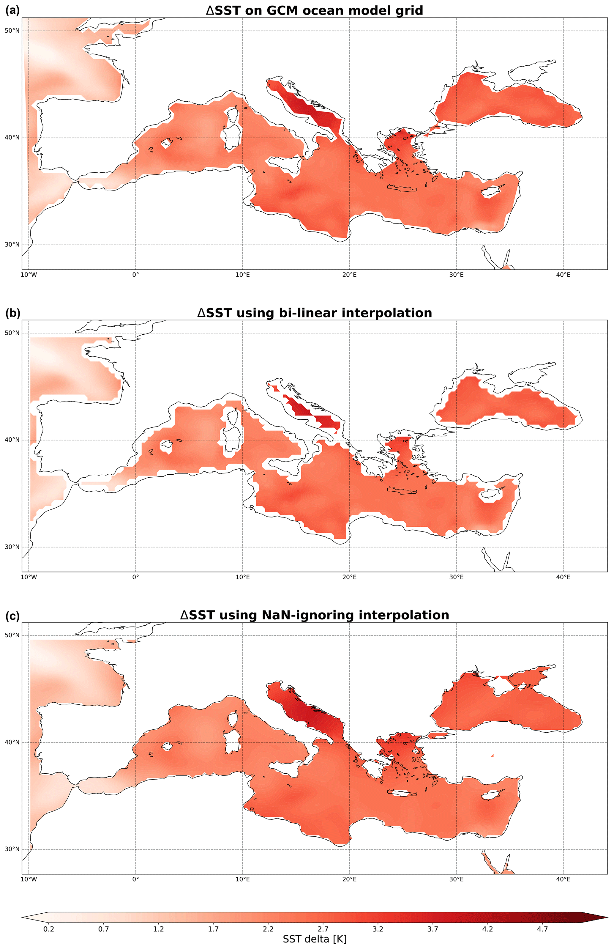
Figure 4 Monthly mean sea surface temperature climate delta (ΔSST) during January obtained from a GCM. (a) ΔSST is shown on the native grid of the GCM ocean model. (b) ΔSST after naive bilinear interpolation onto the reanalysis grid. Information is lost around the coastlines. (c) ΔSST after NaN-ignoring interpolation onto the reanalysis grid. Hereby, additional detail near the reanalysis coastlines is achieved through extrapolation of the original ΔSST. Further information about the data and interpolation used is given in Table A1.

2.8 Pressure adjustment

The most demanding task of the PGW procedure is the pressure adjustment. There are two factors to be considered. First, as the troposphere warms, the air will expand, and tropospheric pressure levels are lifted correspondingly. This effect requires a pressure adjustment in the PGW approach (Schär et al., 1996). The magnitude of this effect can be estimated from the hydrostatic relation (5). For further consideration, let us consider the 500 hPa surface. If the air below is uniformly warmed by ΔT, the altitude of the 500 hPa surface will be lifted according to

$$\begin{array}{}\text{(11)}& {\displaystyle \frac{\mathrm{\Delta }z}{\mathrm{\Delta }T}}={\displaystyle \frac{R}{g}}\ln {\displaystyle \frac{\mathrm{1000}\mathrm{hPa}}{\mathrm{500}\mathrm{hPa}}}\approx \mathrm{20}\mathrm{m}{\mathrm{K}}^{-\mathrm{1}}.\end{array}$$

Thus, for each degree of warming, the 500 hPa surface is lifted by about 20 m.

Second, climate change is associated with circulation and pressure changes. In our PGW approach, these changes are contained in Δϕ_ref=Δϕ(p_ref). These changes include geographical variations which must also be accounted for.

In pressure coordinates the pressure adjustment is rather straightforward. However, in hybrid (sigma/pressure) vertical coordinates as used by ERA, adjusting the pressure consistently is not straightforward. In particular, the pressure of the coordinate levels depends on the surface pressure. The unknown in this process is the change in surface pressure Δp_sfc. An iteration is required with the goal that the resulting change in geopotential height Δϕ_ref at the reference pressure level p_ref agrees with that provided by the GCM.

We start the iteration with $p^{\prime }{{}_{\text{sfc}}}^{n=\mathrm{0}}:=p_{\text{sfc}}$, where n denotes the iteration parameter. The iteration is conducted for each grid column, and each iteration step involves the following computations.

• Step 1. Computation of q_v from temperature and relative humidity in ERA. This is needed as our procedure uses ΔRH rather than Δq_v (see Sect. 4.3). This is followed by the computation of the virtual temperature T_v which appears in the hydrostatic relation.

• Step 2. Reconstruction of the geopotential using the same procedure as described in Sect. 2.4 above. In essence, this is the vertical integration of the hydrostatic equation expressed by Eq. (6).

• Step 3. Computation of ${\mathit{\varphi }}^{\prime }{{}_{\mathrm{ref}}}^n$ at the reference pressure level p_ref using Eq. (7). Note that this requires the computation of k^*, an integer that may change with the iteration.

We may write the iteration step of the pressure adjustment as

$$\begin{array}{}\text{(12)}& {\mathit{\varphi }}^{\prime }{{}_{\mathrm{ref}}}^n=f\left(p^{\prime }{{}_{\text{sfc}}}^n\right).\end{array}$$

There are different ways to advance the iteration. Simple scaling suggests proceeding with

$$\begin{array}{}\text{(13)}& p^{\prime }{{}_{\text{sfc}}}^{n+\mathrm{1}}-p^{\prime }{{}_{\text{sfc}}}^n=-\mathit{\alpha }{\displaystyle \frac{p^{\prime }{{}_{\text{sfc}}}^n}{RT{}_{\text{sfc}}^{\prime }}}\left({\mathit{\varphi }}^{\prime }{{}_{\mathrm{ref}}}^n-{\mathit{\varphi }}^{\prime }{}_{\mathrm{ref}}\right),\end{array}$$

with the target geopotential ${\mathit{\varphi }}_{\mathrm{ref}}^{\prime }$ (obtained from Eq. 9) and a proportionality factor α≤1. Using α=0.95 and ${\mathit{\varphi }}^{\prime }{{}_{\mathrm{ref}}}^n-{\mathit{\varphi }}^{\prime }{}_{\mathrm{ref}}\le \mathrm{0.15}$ m² s⁻² as convergence conditions, the iteration usually requires less than 10 steps to converge. Upon completion of this iteration, the PGW-shifted ERA reanalysis may be used for the computation of the lateral boundary conditions and the execution of the PGW simulation (Fig. 2).

2.9 Refined pressure adjustment

2.9.1 Refined vertical interpolation

In Sect. 2.6 we have simplified the interpolation in the vertical when transforming Δ_GCM to Δ_ERA by assuming that changes in pressure are small. In principle, one can relax this assumption by including the application of the Δ (see Sects. 2.6 and 7) in the iteration loop discussed in Sect. 2.8. We have tested this procedure but did not find significant improvements. Indeed, likely other aspects of the procedure (such as using monthly mean changes or the vertical resolution of the climate deltas) are more important than the details of the vertical interpolation. Moreover, in the lower troposphere the effect of the pressure adjustment is small according to Eq. (11).

2.9.2 Use of multiple geopotential height levels

In the version of the code described above, we use one specific p_ref level to account for the changes in geopotential. This level must be chosen at a height which is above all topographies in the computational domain. If there is high topography within the domain, one might be forced to use an elevated level at the 500 hPa level or even higher. This implies that the vertical integration in step 2 of the iteration (see Sect. 2.8) must cover a deeper layer and might suffer from a larger error (see below). For this reason, the code enables the use of multiple reference levels. In essence, the lowermost pressure level located above the topography in a specific ERA grid column is then used.

The pressure adjustment is affected by the number of pressure levels of the climate deltas. For instance, when using AMON data, there are 19 pressure levels in total, of which there are only 6 levels between 1000 and 500 hPa. This has implications for the accuracy of the pressure adjustment via the integration of the geopotential. While in the GCM Δϕ_ref in Eq. (9) is integrated on the native vertical grid of the GCM (using T and q_v on all GCM levels), the integration of ${\mathit{\varphi }}_{\mathrm{ref}}^{\prime }$ used in Eq. (13) is an approximation and depends on the vertical resolution of ΔT and Δq_v below p_ref. An illustration of this is shown in Fig. 5 for both AMON and EMON data in a marine trade-wind domain. When using the low-resolution AMON data, the poorly represented jump in ΔT and Δq_v across the trade-wind inversion leads to errors in the integration of ${\mathit{\varphi }}_{\mathrm{ref}}^{\prime }$ and in the adjusted surface pressure. Such uncertainties are particularly important in the tropics, where small horizontal gradients in geopotential can drive significant circulations. The problem is further illustrated in Fig. 6, showing the deviation in geopotential height at different pressure levels between two PGW setups with EMON and AMON climate deltas. The pressure adjustment is done with one reference pressure level at 500 hPa. Consequently, the deviation (EMON–AMON) is very small at 700 hPa but increases towards the surface and towards the model top. The error resulting from the trade-wind inversion is clearly visible in Fig. 6a.

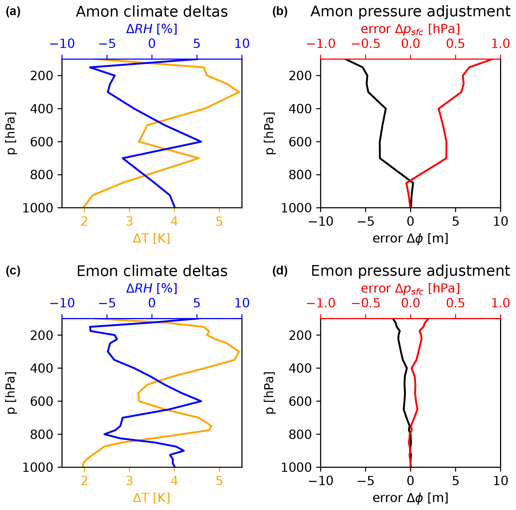
Figure 5 Illustration of the pressure adjustment using AMON (a, b) and EMON (c, d) pressure level data with 19 and 27 pressure levels, respectively. The analysis is done for a $\mathrm{2}{}^{\circ }\times \mathrm{2}{}^{\circ }$ box over the subtropical South Atlantic at a particular point in time. Panels (a) and (a) show ΔT and ΔRH, and panels (a) and (d) show the integration error in Δϕ when integrated from the surface (sfc) to pressure p and the error in Δp_sfc resulting from the pressure adjustment for a given reference pressure level p_ref (y axis). The adjustment based on AMON data has large uncertainties (error in Δp_sfc) for p_ref<850 hPa due to the pronounced trade-wind inversion. Further information about the data used and the error computation is given in Table A1.

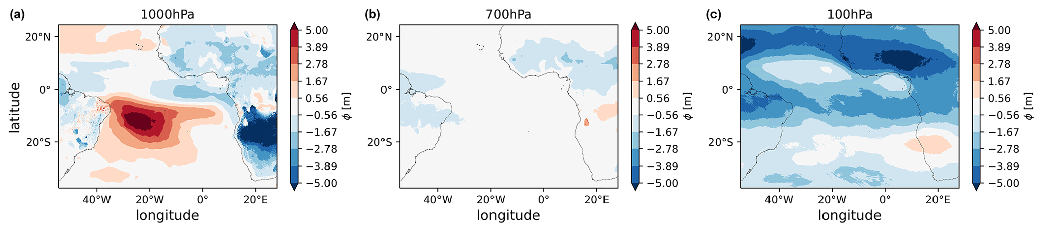
Figure 6 Difference in the geopotential height (m) between PGW boundary conditions derived using EMON and AMON data, respectively, at 1000 hPa (a), 700 hPa (b), and 100 hPa (c) at one specific time. In both cases, the pressure adjustment is done with one fixed reference pressure level at 500 hPa. Further information about the data used is given in Table A1.

3 Comparison with standard dynamic downscaling

The key question is whether the simplifying assumptions made with the PGW methodology are sufficiently valid. To test this question, we present a detailed intercomparison of climate change scenarios derived from both the conventional and PGW methodologies. In the intercomparison, the conventional methodology considers multi-decade-long SCEN and HIST simulations for recent and end-of-century periods driven by a GCM, while the PGW scenario uses the same large-scale forcing but applies it to modify a CTRL simulation. Further details about the simulations, such as information on emission scenarios, the time periods considered, and the driving simulations, can be found in Table A1.

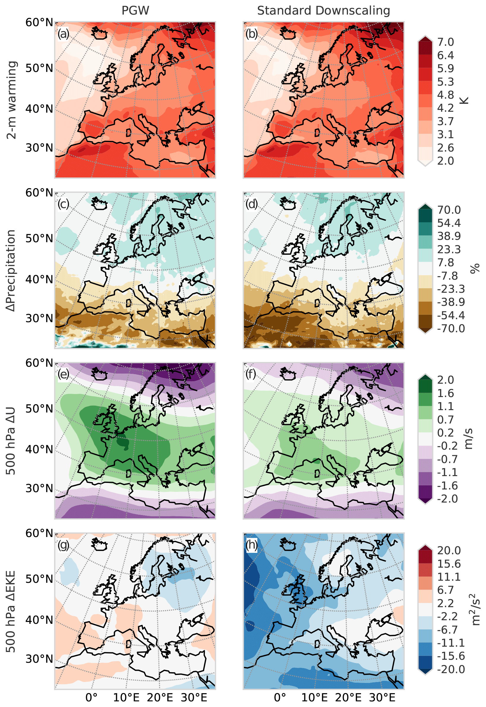
Figure 7 Comparison of annual mean climate change projections derived from (left) PGW and (right) standard downscaling methodologies for the time periods 2070–2099 versus 1971–2000 using an RCP8.5 emission scenario. (a–b) 2 m temperature change, (c–d) mean precipitation change, (e–f) mid-tropospheric zonal wind change, and (g–h) mid-tropospheric change in eddy kinetic energy (calculated as $\mathrm{0.5}\left(\right(u-\stackrel{\mathrm{‾}}{u}{)}^{\mathrm{2}}+(v-\stackrel{\mathrm{‾}}{v}{)}^{\mathrm{2}})$, with (u,v) the instantaneous value of the wind and $(\stackrel{\mathrm{‾}}{u},\stackrel{\mathrm{‾}}{v})$ the 30-year mean thereof). Details on the simulation setup can be found in Table A1.

In Fig. 7, we show a direct comparison of transient RCM simulations with corresponding PGW simulations. We aimed to assess how similar to a transient simulation a PGW simulation can be. Therefore, to derive the PGW simulation, we used the transient simulation to provide Δ with Eq. (2). We also used the historical period (1971–2000) from the transient simulation as a basis for the PGW (CTRL in Eq. 1). This means that, in Fig. 7, the future simulation differs (GCM-driven versus PGW), but the historical simulation is identical in both cases. The details on the models used can be found in Table A1.

We observe that the temperature projections in the transient simulations and the PGW simulations are virtually identical (Fig. 7a–b). Also, the PGW approach leads to similar projections for precipitation (Fig. 7c–d) and mean wind (Fig. 7e–f). The eddy kinetic energy (EKE, defined as $\mathrm{0.5}\left(\right(u-\stackrel{\mathrm{‾}}{u}{)}^{\mathrm{2}}+(v-\stackrel{\mathrm{‾}}{v}{)}^{\mathrm{2}})$ and computed as in Brogli et al., 2019b), a proxy for cyclone activity, clearly decreases in the GCM-driven simulations (Fig. 7h), while in the PGW, EKE does not substantially change (Fig. 7g). As discussed earlier, this is the expected behavior, since a historical simulation is merely modified in the PGW approach and the sequence of cyclones entering the domain does not change. More specifically, the climate change signal exhibits polar amplification and baroclinicity, consistent with a reduction in eddy kinetic energy (Fig. 7h).

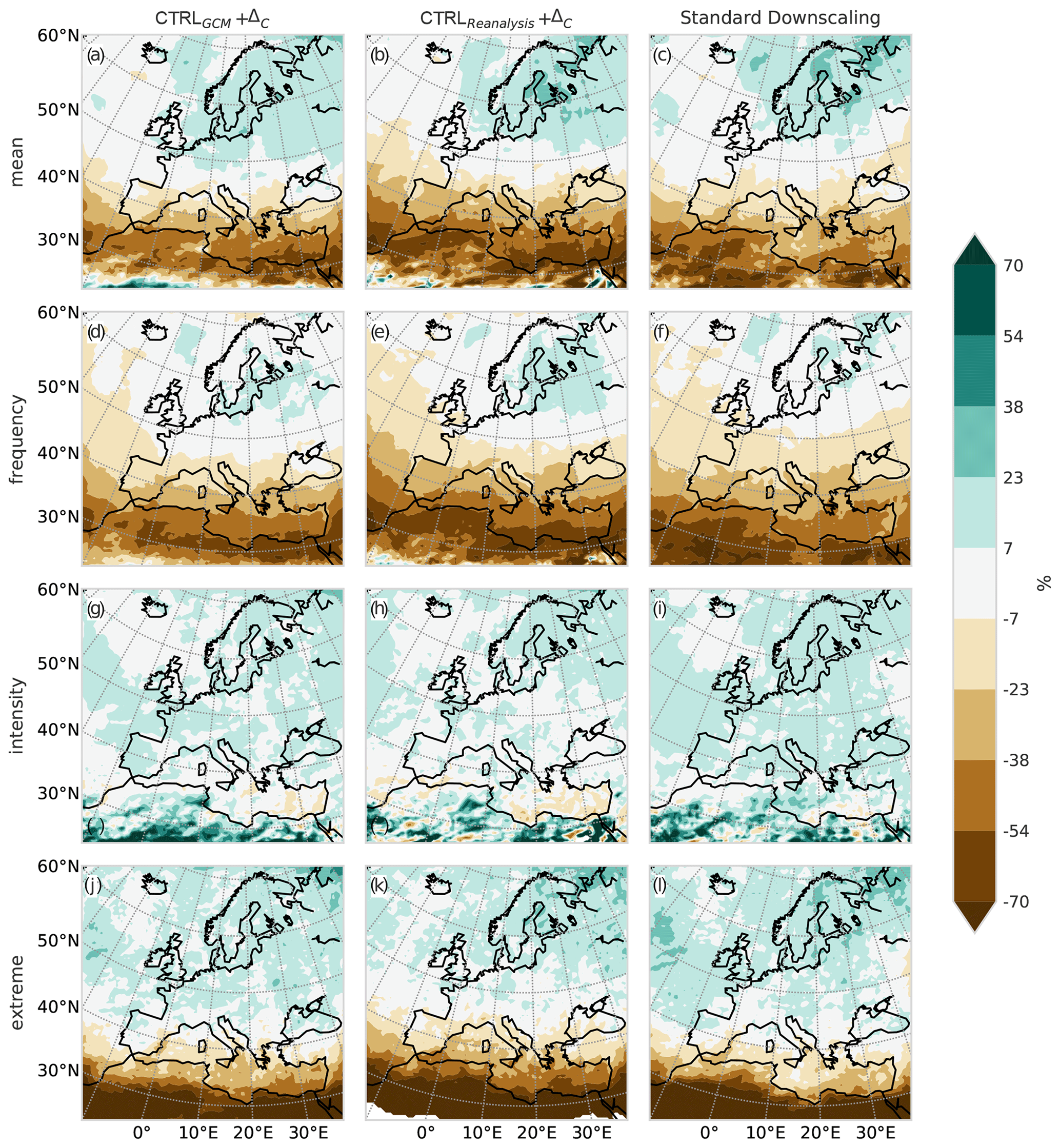
Figure 8 Similar to Fig. 7 but for annual mean changes in (a–c) mean precipitation, (d–f) precipitation frequency (days with precipitation ≥ 1 mm), (g–i) precipitation intensity (precipitation amount on days with ≥ 1 mm), and (j–l) extreme precipitation (99th percentile of all days), for three climate change projections. The first column (a, d, g, j) shows a GCM-driven CTRL simulation modified using the PGW approach. The second column (b, e, h, k) shows an ERA-Interim-driven CTRL simulation modified using the PGW approach. The third column (c, f, i, l) shows the standard GCM-driven transient climate simulation. Details on the models used are in Table A1.

Since the majority of PGW use cases employ a reanalysis-driven historical simulation, we next compare a reanalysis-based PGW simulation to a GCM-based PGW simulation and to standard downscaling. Figure 8 shows changes in precipitation statistics in these three types of simulations (three columns). Independently of the choice of downscaling strategy, the projected changes in precipitation are extremely similar and show a pattern that is consistent with previous analyses of large simulation ensembles (Rajczak and Schär, 2017). This is not only true for mean precipitation changes, but also for changes in the intensity and frequency and extreme indices. The differences between the two PGW versions (columns 1 and 2) are entirely due to the use of another historical simulation, while the Δ used in both PGW simulations shown in Fig. 8 is identical. Although similar, some subtle differences in projected precipitation changes are visible. It is hard to tell which of the scenarios should be closest to reality. On the one hand, the reanalysis-driven historical simulation has the smallest bias. On the other hand, the standard downscaling approach most consistently accounts for large-scale climate changes.

4 Sensitivity tests

During the development of our PGW simulations, we performed multiple sensitivity tests related to the design of the workflow which will be presented in this section.

4.1 Hydrostatic balance

We maintain the hydrostatic balance in our PGW simulations by adjusting the pressure in each boundary condition field according to Sect. 2.8. Figure 9 demonstrates that doing so matters for the simulation result. More specifically, we see that in a historical simulation for November 2004 over the tropical Atlantic the mean sea level pressure is ∼ 1010 hPa. If we raise the temperature in the same simulation and use the same pressure at the lateral boundaries, the mean sea level pressure drops by 10–15 hPa within the domain, which is no longer realistic. Note that this implies a discontinuity at the lateral boundaries, which is visible by close inspection in Fig. 9b. By readjusting the pressure, the mean sea level pressure values remain reasonable even when the temperature is raised (Fig. 9c).

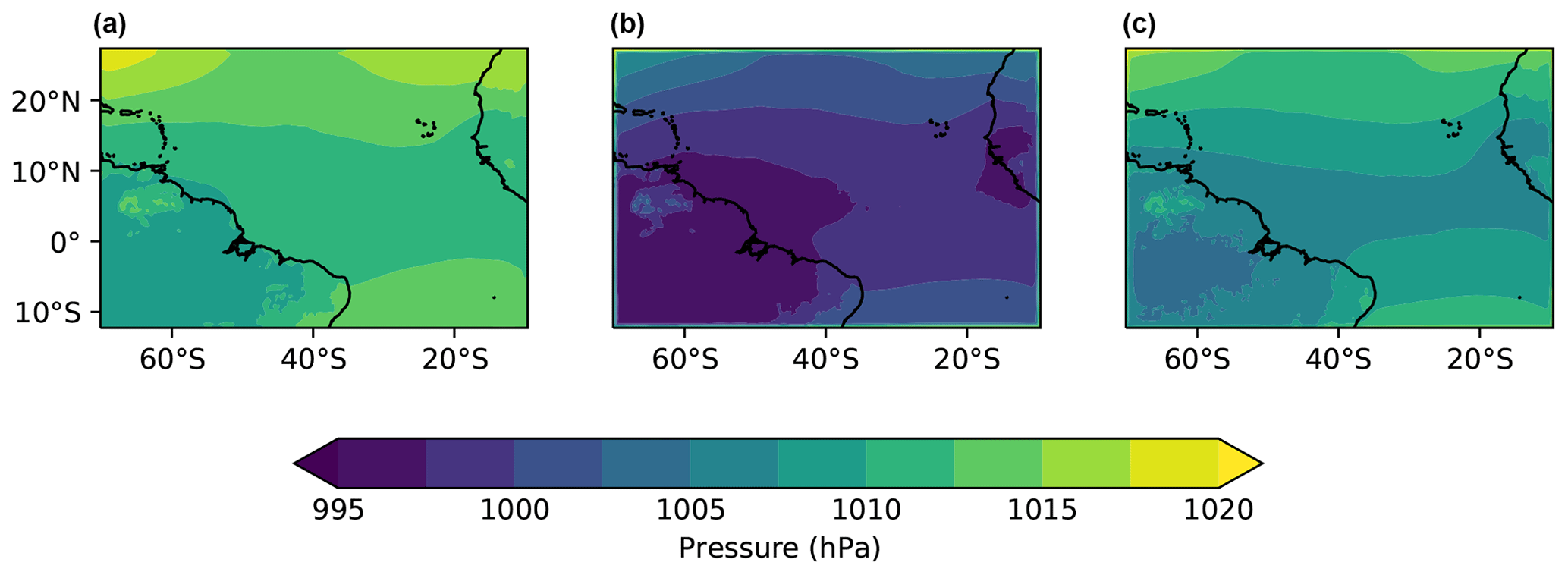
Figure 9 Mean sea level pressure in PGW simulations and the effect of maintaining the hydrostatic balance. (a) Mean sea level pressure in the reanalysis-driven CTRL simulation of the month of November 2004. Panel (c) shows the PGW simulation where the full PGW procedure described in Sect. 2 was followed, including the pressure adjustment. (b) As (c) but using a simplified procedure where the pressure at the lateral boundaries was left unchanged. The computational domain covers the tropical Atlantic. Note the significant differences between panels (b) and (c), highlighting the importance of the pressure adjustment. Technical simulation details are in Table A1.

4.2 Thermal wind balance

Figure 10 presents the effects of prescribing wind changes consistent with the thermal wind balance at the lateral boundaries of PGW simulations. We compare a simulation that includes the full PGW methodology as described in Sect. 2 against one where the three-dimensional temperature changes were applied but not the corresponding changes in mean wind. We compare the two simulations in terms of EKE. It is evident that the response deteriorates when the thermal wind balance at the lateral boundaries is violated by making temperature changes without corresponding wind changes (Fig. 10b). This increase in EKE can physically be interpreted as resulting from a geostrophic adjustment process. Also, when not balancing the wind changes, the resulting strong EKE change has the opposite sign of what is seen in dynamic downscaling (Fig. 10c). Note that wind changes need to be made along with temperature changes as soon as spatial gradients in the temperature change are prescribed. In idealized PGW settings where a spatially uniform temperature change is imposed, the wind can be left unchanged.

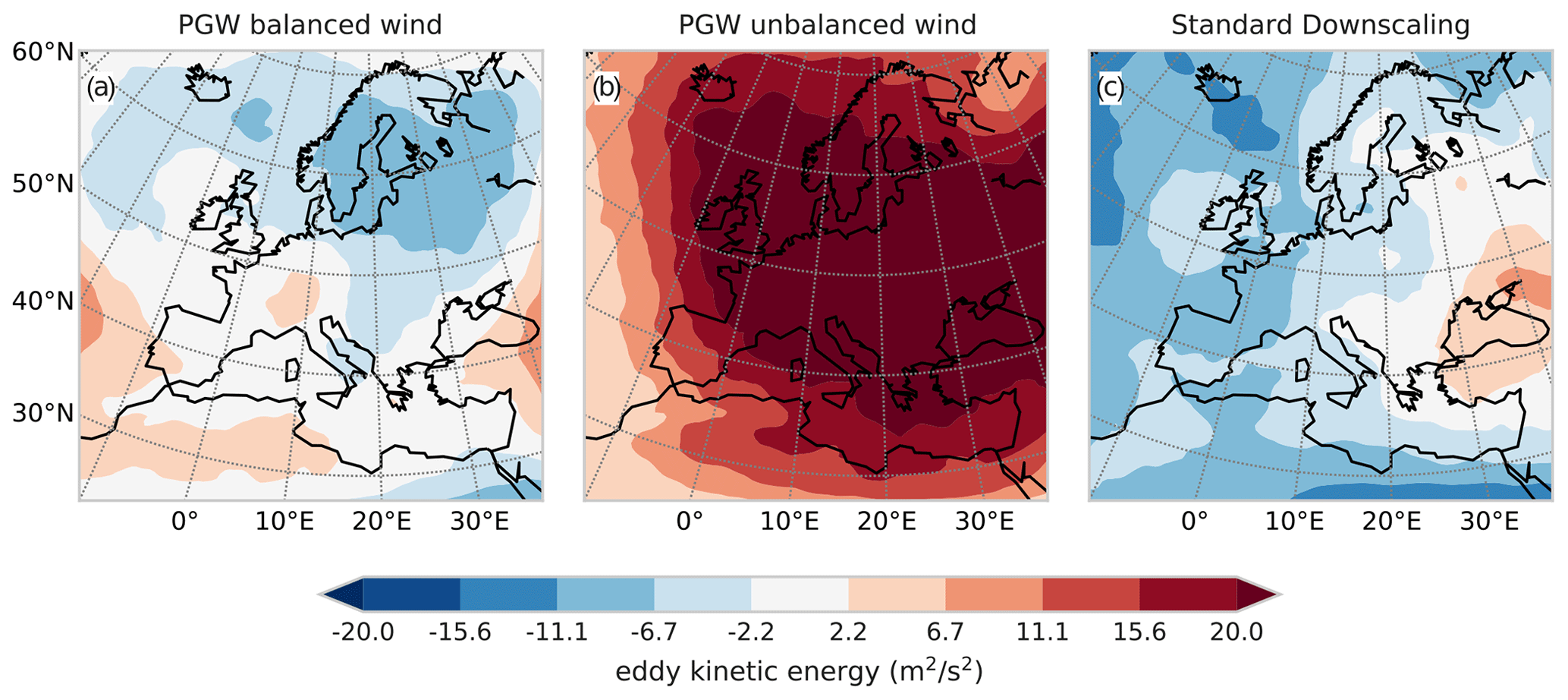
Figure 10 Effect of the thermal wind balance on changes in 500 hPa eddy kinetic energy (EKE) in PGW simulations. (a) PGW simulation where both changes in temperature and wind were made at the lateral boundaries and therefore the thermal wind balance was maintained. (b) PGW simulation where the temperature at the lateral boundaries was changed without corresponding changes in wind. (c) EKE changes from dynamically downscaling the same GCM. Details on the simulations in Table A1.

4.3 Changes in humidity

It may be surprising that PGW4ERA5 relies on changes in RH to modify the moisture in the PGW framework, even though most RCMs use specific humidity (q_v) as a prognostic and output variable. As shown in Fig. 11, a direct modification of the boundary conditions with q_v regionally leads to artificial supersaturation along the model boundary. This supersaturation leads to an unrealistic precipitation band along the model boundary and also affects precipitation in the interior of the domain (Fig. 11b, c). This problem is avoided by using RH to modify the moisture (Fig. 11a).

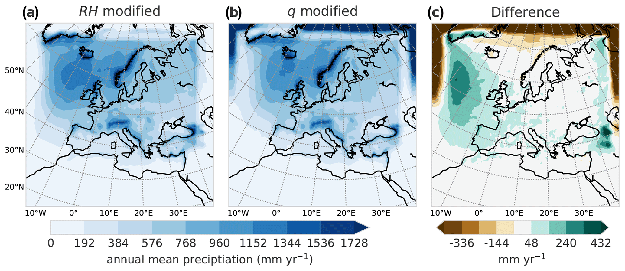
Figure 11 Different modifications of humidity in PGW simulations and their effect on annual mean precipitation between 2070 and 2099. (a) Humidity is changed according to the GCM-projected changes in relative humidity. (b) Humidity is changed according to projected changes in specific humidity. (c) Difference between panels (a) and (b). The panels show the whole computational domain, including the lateral relaxation boundary zone. Details on the models used are given in Table A1.

How can we explain the difference between these approaches? The ΔRH for humidity at a certain time step is representative of the climatological change at the time of the year. Thus, virtually the same change is imposed, for example, during the night (comparably cool and low moisture-holding capacity) and during the day (warmer and higher moisture-holding capacity) and similarly during cold and warm days. During cool periods, it is easy to heavily oversaturate the atmosphere at the lateral boundaries when an absolute change in q_v is imposed. In contrast to q_v, RH changes little under climate change, as it intrinsically contains information on the relative saturation of the air. Thus, the changes in RH in the PGW framework can be understood as deviations from the expectations based on the Clausius–Clapeyron relation, and they are typically small (10 % or less).

4.4 Temporal resolution of input data

The mean annual cycle of Δ can be computed based on monthly mean or daily mean input data in PGW4ERA5 (see Sect. 2.5). Our tests have shown that the choice of the procedure has only a minor effect on the simulation results on climatological timescales. An example of 30-year annual mean temperature is shown in Fig. 12, where we observe that the mean pattern of future temperature is almost indistinguishable when comparing a PGW simulation based on daily and monthly mean input. The small differences between the approaches (<0.1 K) are likely due to chaotic dynamics and associated sensitivities due to small changes (Fig. 12c). These same results also hold for precipitation changes (not shown).

Figure 12 Annual mean temperature distribution for 2070–2099 in a PGW simulation depending on the selected temporal resolution of the input data. (a) PGW simulation where smoothed daily changes have been used to modify the lateral boundaries (blue line in Fig. 3). (b) PGW simulation where a linear interpolation between monthly mean changes was applied (orange line in Fig. 3). (c) Difference between panels (a) and (b).

Based on these tests, using monthly mean input data is the preferable strategy in the majority of PGW applications. That is because it is less data- and computing-intensive to process the monthly mean values for SCEN and HIST. Still, if daily input data (with the same or higher vertical resolution) are readily available, it may make sense to use them.

5 Conclusions

We have shown that the pseudo-global warming (PGW) approach is an alternative method for providing climate scenarios using regional climate models. If adequately designed, PGW simulations provide plausible future climate change projections that agree well with traditional dynamic downscaling. The methodology uses global model output and accounts for large-scale changes in temperature and humidity as well as monthly-mean circulation changes. However, it does not account for changes in large-scale interannual variability (e.g., changes in the frequency of El Niño). In our paper we present a detailed intercomparison against the standard GCM-RCM downscaling approach. For most of the impact-oriented fields, such as surface temperature and precipitation changes as well as precipitation indices relating to heavy and extreme precipitation events, the differences between the two approaches are small and sometimes barely noticeable. As one would expect, there are some minor changes in upper-level synoptic activity, but these do not appear to significantly affect the impact-oriented output parameters.

PGW simulations can be attractive for reducing the computational burden of climate projections, offer flexibility in the design of future projections, and allow future simulations based on reanalysis-driven evaluation runs.

Still, expertise is required to prepare a PGW simulation. With an extended description and evaluation of the methodology and by providing the PGW4ERA5 software, this work intends to support the future use of PGW simulations. The workflow is generalized where possible and completely written using the widely used Python programming language. The interface to the RCM is provided on the level of the ERA5 reanalysis; i.e., the software provides modified ERA5 reanalysis files.

Appendix A

(Leutwyler et al., 2017)(Dee et al., 2011)(Rockel et al., 2008)(Stevens et al., 2013)(Gutjahr et al., 2019)(Meinshausen et al., 2020)(The HadGEM2 Development Team, 2011)

Table A1 Most figures presented in this article show climate simulations. This table contains details on the setup of the simulations shown in the figures. The first column indicates the figure for which the information is shown. The second column shows the panels or parts of the figures for which the information is valid. The description of the simulations is in the third column.