Cell tracking of convective rainfall: sensitivity of climate-change signal to tracking algorithm and cell definition (Cell-TAO v1.0)

Lagrangian analysis of convective precipitation involves identifying convective cells (“objects”) and tracking them through space and time. The Lagrangian approach helps to gain insight into the physical properties and impacts of convective cells and, in particular, how these may respond to climate change. Lagrangian analysis requires both a fixed definition of what constitutes a convective object and a reliable tracking algorithm. Whether the climate-change signals of various object properties are sensitive to the choice of tracking algorithm or to how a convective object is defined has received little attention. Here we perform ensemble pseudo-global-warming experiments at a convection-permitting resolution to test this question. Using two conceptually different tracking algorithms, Lagrangian analysis is systematically repeated with different thresholds for defining a convective object, namely minimum values for object area, intensity and lifetime. It is found that the threshold criteria for identifying a convective object can have a strong and statistically significant impact on the magnitude of the climate-change signal, for all analysed object properties. The tracking method, meanwhile, has no impact on the climate-change signal as long as the precipitation data have a sufficiently high temporal resolution: in general, the lower the minimum permitted object size is, the higher the precipitation data's temporal resolution must be. For the case considered in our study, these insights reveal that irrespective of the tracking method, projected changes in the characteristics of convective rainfall vary considerably between cells of differing intensity, area and lifetime.

1 Introduction

Lagrangian analysis of convective precipitation offers an alternative to the more common Eulerian approach, in which precipitation is considered at a fixed location. In the Lagrangian framework, often referred to as “cell”, “storm”, “feature” or “object-oriented” tracking, convective “objects” are identified and then tracked through space and time. The approach has historically been mostly used in radar-based nowcasting, in which the location of convective cells is forecast based on Lagrangian advection from previous radar scans (Dixon and Wiener, 1993; Golding, 1998; Mandapaka et al., 2012; Novo et al., 2014). The Lagrangian approach furthermore allows for the properties of convective objects to be measured during the object's life cycle. Characterizing these properties – e.g. area, mean or maximum intensity, and distance travelled – has applications in both model evaluation and climate-change and impact studies. In the former, aspects of model-simulated convective precipitation which would not be discernible from Eulerian analysis – e.g. cell areal extent, lifetime and distance travelled – can be compared with radar-based observations (Caine et al., 2013; Brisson et al., 2018; Purr et al., 2019; Caillaud et al., 2021; Raupach et al., 2021), avoiding the double-penalty problem and potentially revealing previously unknown model strengths or weaknesses (Clark et al., 2014; Skinner et al., 2018). For climate-change studies, Lagrangian techniques can identify the relative changes in different storm properties, thus offering additional insight into the physical mechanisms underlying projected future changes in convective precipitation (Purr et al., 2021; Prein et al., 2017; Poujol et al., 2020a). For impact studies, multiple factors such as storm motion, translation speed and spatiotemporal variability affect the drainage response of a catchment (Amengual et al., 2021): object-oriented analysis allows for these factors to be quantified.

The many object-based algorithms used to track convective precipitation employ a number of different approaches, which include (i) pattern-matching-, (ii) overlap- and (iii) advection-based techniques, as well as combinations of the aforementioned. In pattern-matching approaches (Einfalt et al., 1990; Dixon and Wiener, 1993), the precipitation fields at successive time steps are compared and object motions are determined based on spatial correlation or some other optimization method which matches objects with similar characteristics. With overlap-based methods (Morel and Senesi, 2002; Hering et al., 2004; Davis et al., 2006), the aim is to find object footprints which are contiguous in both space and time (i.e. spatial overlap at successive time steps). This approach may, in certain cases, be unsuitable for application with radar data: if the scans are too infrequent, contiguity will be lost; even in models, very small objects may also not overlap at successive time steps. In the advection-based approach, the expected position of the object is estimated based on Lagrangian extrapolation from the previous time step(s). Extrapolation may be based on, for example, mid-tropospheric flow (Purr et al., 2019; Brendel et al., 2014; Moseley et al., 2013), optical flow methods (He et al., 2019; Muñoz et al., 2018; Woo and Wong, 2017) or advection of some otherwise computed velocity field (Stein et al., 2014; Germann and Zawadzki, 2002). The approach may be unsuitable in back-building situations (Parodi et al., 2017), where cold-pool outflows cause the convective system to propagate against the direction of flow.

The desire to track convective objects naturally raises the question of what exactly a convective object is and how it should be defined. For tracking purposes, convective objects are typically defined based on exceedance of three threshold minima: (1) minimum precipitation intensity, (2) minimum area and (3) minimum lifetime. Some tracking algorithms employ a fourth criterion, whereby precipitation must also be identifiable as convective, e.g. based on cloud-top temperatures (Chen et al., 2019), precipitation gradients (Brendel et al., 2014) or mid-tropospheric dynamics (Poujol et al., 2020b). The choices of the aforementioned thresholds vary considerably in the literature: minimum intensities from 0.1 mm h⁻¹ (Li et al., 2020) to 30 mm h⁻¹ (Caillaud et al., 2021); area thresholds as low as 2 or 4 km² (Moseley et al., 2013; Stein et al., 2014) and as high as 32 000 km² (Prein et al., 2017); and time thresholds of 10 min (Moseley et al., 2013), 30 min (Burghardt et al., 2014) or even longer in low-temporal-resolution data (Li et al., 2020). While it seems obvious that the choice of how to define a convective object will impact the climatological statistics of certain object properties (e.g. Müller et al., 2022), what is not clear is if these choices may also impact the climate-change response of convective objects' characteristics. The same question may also be posed of the chosen tracking method.

To investigate these questions, we employ the pseudo-global-warming (PGW) method (Schär et al., 1996) to perform high-resolution ensemble climate-change simulations with a convection-permitting model (CPM). Our PGW ensemble covers a 2-week period of exceptionally high thunderstorm activity over central Europe (Piper et al., 2016). CPMs offer an ideal tool to investigate such questions, as they explicitly represent deep convection. In our study region, CPMs have been shown to add value for the representation of both the diurnal convective cycle (Meredith et al., 2021; Brisson et al., 2016b) and intense convective precipitation (Fosser et al., 2015; Knist et al., 2018). Importantly for the tracking of convective objects, CPMs – here, the COSMO-CLM (Consortium for Small-scale Modeling in CLimate Mode; Rockel et al., 2008) – can realistically represent many aspects of subhourly precipitation from both Eulerian (Meredith et al., 2020) and Lagrangian (Brisson et al., 2018; Purr et al., 2019) perspectives. Using two different tracking methods, based on the overlap and advection approaches, we track all convective objects in the aforementioned (present and future) PGW ensemble. The tracking is repeated using different options for defining a convective object: the thresholds of minimum intensity, area and lifetime discussed above are systematically varied. The aim is to see how sensitive the warming response of different object characteristics is to the chosen tracking method and the manner in which a convective object is defined.

In the main Results section (Sect. 4), our purpose is to pose the following question. In the presence of a climate-change signal, can projected changes in the characteristics of convective cells be sensitive to the choice of tracking algorithm or to how a convective object is defined? We are thus interested in differences in the climate-change signal, rather than precisely determining the magnitude of convective objects' response to climate change in our region. In Sect. 5, we use our PGW simulations to explore how – based on any sensitivities identified in the preceding section – Lagrangian projections might be analysed so that projections are less sensitive to the criteria used for detecting a convective object.

2 Study period

Our study makes use of a 2-week period of unusually high convective activity over Germany, from 26 May to 9 June 2016 and analysed in detail in Piper et al. (2016). The exceptional number of thunderstorms over an extended period led to flash flooding and serious structural damage in many locations (e.g. Bronstert et al., 2018). The study period can be roughly split into two parts: a first part in which convection was caused by a strong synoptic forcing (Fig. 1a) and a second in which weak forcing (Fig. 1b) gave rise to a daily cycle of instability building over large areas, followed by intense convection in the late afternoon and evening (Hirt and Craig, 2021). Owing to its elevated levels of both weakly and strongly forced convection, the period has previously been used as a test case in numerous studies of convection in kilometre-scale models (Baur et al., 2018; Rasp et al., 2018; Keil et al., 2019; Hirt et al., 2019; Hirt and Craig, 2021). The period of strong synoptic forcing included south-easterly advection of warm and moist air into Germany and large-scale uplift from a strong potential vorticity anomaly on 29 May, followed by a number of near-stationary surface lows over central Europe under a 500 hPa cut-off low. The weakly forced convection occurred under an upper-level stationary ridge. Further discussion is available in the aforementioned references.

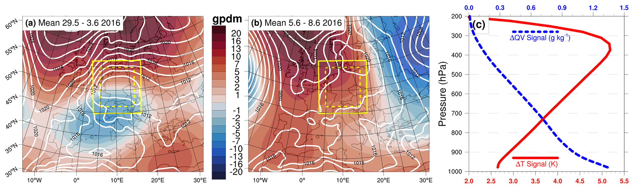
Figure 1 The 500 hPa geopotential height anomaly (gpdm, shading; reference is the 1979–2015 mean) and sea level pressure (hPa, white lines) averaged over the periods (a) 29 May–3 June and (b) 5–8 June 2016. The maps cover the spatial extent of the 0.11^∘ simulation domain, and the solid and dashed yellow lines mark the 0.025^∘ simulation domain and analysis region, respectively. (c) The climate-change signals of temperature (T; red line) and specific humidity (QV; blue line) added to the initial and boundary conditions of the 0.11^∘ PGW simulations. The signal is computed based on an area average over the 0.11^∘ domain; change profiles for winds and pressure, as well as equivalent plots on height levels, are presented in Fig. S1.

3 Methods

3.1 Climate simulations

We perform 18-member ensemble regional climate model (RCM) simulations of our study period using the PGW approach (Schär et al., 1996) at a convection-permitting resolution (0.025^∘, ∼2.8 km). In the PGW approach, an event or period is first dynamically downscaled from a reanalysis under present conditions. The downscaling is then repeated with altered RCM initial and boundary conditions which reflect projected changes in the boundary variables (or a subset thereof). This approach has previously been employed in numerous studies on both climate and event-based timescales (Prein et al., 2017; Lackmann, 2013; Rasmussen et al., 2014; Kröner et al., 2017; Keller et al., 2018; Hibino et al., 2018). All of our simulations are performed with COSMO-CLM (Rockel et al., 2008), version 5.0_clm16.

The first modelling step (present climate) involves multi-reanalysis downscaling of ERA-Interim (Dee et al., 2011) and MERRA-2 (Modern-Era Retrospective analysis for Research and Applications; Gelaro et al., 2017) to 0.11^∘ resolution from 26 May 2016 to 9 June 2016 over a pan-Europe domain (Fig. 1). An ensemble is then created using the domain-shift technique (e.g. Rezacova et al., 2009; Pardowitz et al., 2016; Noyelle et al., 2019). In this approach, a central domain is defined and the domain centre is systematically shifted five grid cells (∼0.55^∘) in the cardinal and ordinal directions N, NE, E, SE, S, SW, W and NW, giving perturbed initial and boundary conditions for each ensemble member (see Rezacova et al., 2009, or Mazza et al., 2017, for illustrative schematics). The shifting is performed for both reanalyses, giving in total 18 members for the present climate.

The second modelling step (PGW) involves repeating the 0.11^∘ downscaling with modified boundary conditions based on projected changes under an end-of-century RCP8.5 scenario (Representative Concentration Pathway; Van Vuuren et al., 2011), as described above. This high-end scenario is chosen in order to ensure a strong warming signal as the basis for our sensitivity tests. We derive an ensemble mean climate-change signal from historical (1970–1999) and future (2070–2099) periods based on three 0.11^∘ COSMO-CLM simulations from the EURO-CORDEX experiment (European branch of the Coordinated Regional Climate Downscaling Experiment; Jacob et al., 2014). The three EURO-CORDEX runs were downscaled from CMIP5 (Coupled Model Intercomparison Project; Taylor et al., 2012) simulations of the MPI-ESM-LR (r1; Max Planck Institute Earth System Model – low resolution; Giorgetta et al., 2013), EC-Earth (r12; European community earth system model; Hazeleger et al., 2012) and CNRM-CM5 (r1; Centre National de Recherches Météorologiques climate model 5; Voldoire et al., 2013) global models. A 31 d running mean of the resulting climate-change signal (Fig. 1c) is added to the initial and lateral boundary conditions of our 0.11^∘ simulations for all variables (e.g. temperature, specific humidity, pressure and winds).

Finally, all present and PGW members are further downscaled to 0.025^∘ resolution over the COSMO-DE domain (Fig. 1), giving an 18-member CPM ensemble from 27 May to 9 June 2016 (14 d); for analysis, the first 4 h are discarded for spin-up. Note that the COSMO-DE domain is fixed in space; i.e. it is not shifted like the 0.11^∘ domain. Deep convection is explicitly resolved by the model, while shallow convection is parameterized based on a modified Tiedtke scheme (Tiedtke, 1989). All model settings are taken from the standard configuration of the German Weather Service, and precipitation output is saved every 5 min. Aside from the added value of COSMO-CLM, and CPMs in general, discussed in the Introduction, shortcomings in COSMO-CLM do still remain. Keil et al. (2014) reported insufficient convective triggering under conditions of weak synoptic forcing, while Purr et al. (2019) reported an underestimation of mean precipitation intensity in long-living, extreme convective objects and a general overestimation of the lifetime of convective objects. The results presented below are all based on the 0.025^∘ CPM ensemble.

3.2 Tracking algorithms

We make use of two tracking algorithms. In the first, convective objects are tracked based on advection by the steering flow; we refer to this algorithm as ADV. In the second, convective objects are tracked based on the overlap method; we refer to this algorithm as OVER. These algorithms are chosen (i) because they are representative of two standard approaches to tracking convective objects (i.e. advection- and overlap-based tracking) and (ii) for their low levels of complexity, facilitating generalizability of the results.

The ADV algorithm is based on the method of Brendel et al. (2014), which was developed for tracking convective objects in radar data and was adapted for convection-permitting models by Brisson et al. (2018). The OVER algorithm, on the other hand, is a simple temporal-overlap procedure. The algorithms have been summarized in a schematic (Fig. 2). For both algorithms, non-convective precipitation is first masked out using the method of Poujol et al. (2020b). All precipitation below a chosen threshold (P_min) is also masked out. Objects are then identified as contiguous precipitation areas exceeding a minimum chosen area (A_min), based on the number of grid boxes within the object. Objects whose lifetime is shorter than a chosen threshold (T_min) are discarded, as are objects which are not fully in the domain.

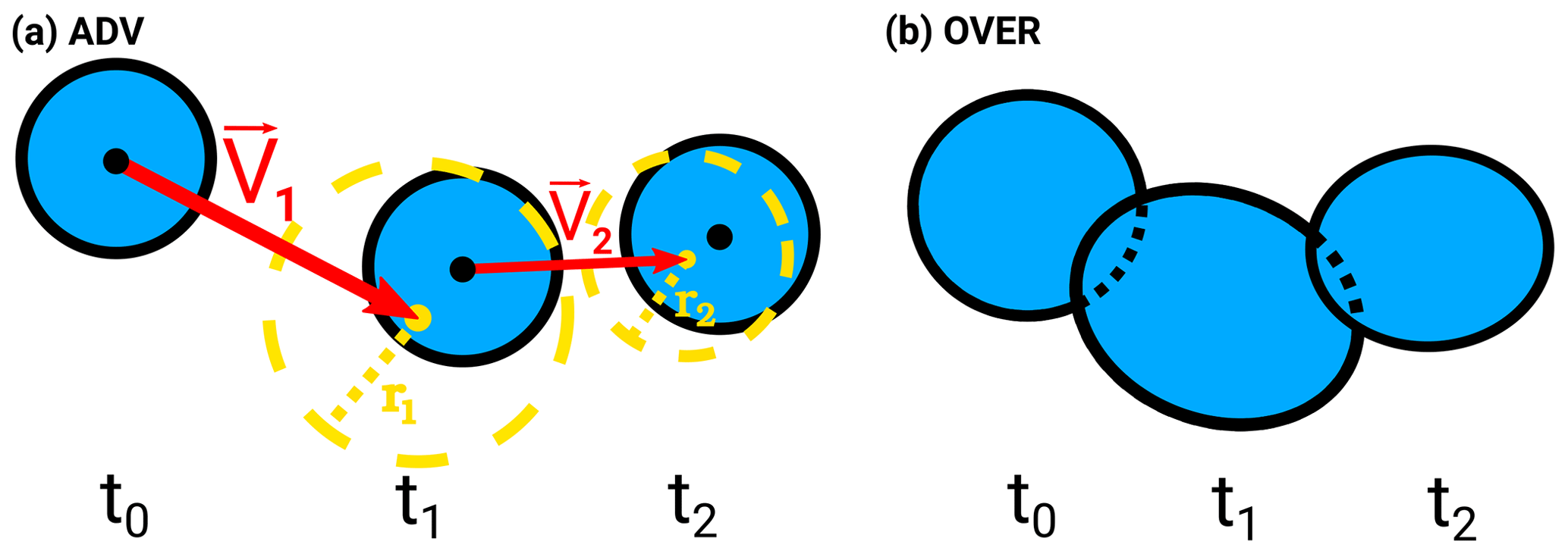
Figure 2 Schematic illustrating the (a) ADV and (b) OVER algorithms. In ADV, the red vectors (emanating from the cell's centre of mass) represent the estimated displacement of the convective cell based on the steering flow. The yellow dashed circle represents the search area, with radius r, in which the displaced cell is sought. The search radius is proportional to the magnitude of the displacement vector. In OVER, the area between the dashed and solid lines marks the cell's area of overlap at consecutive time steps. See also Brisson et al. (2018) for a schematic of the Brendel et al. (2014) algorithm.

In ADV (Fig. 2a), once an object has been identified, its position at the next time step is estimated based on the steering flow, here the wind velocity averaged across the 500, 700 and 850 hPa levels. From the expected location at the next time step, convective objects are searched within a defined search radius whose length is proportional to the wind speed (see Brendel et al., 2014). For the object nearest to the expected location, the procedure is further iterated until no object is found. For object splits, the object nearest to the expected location is chosen, while the remaining object(s) is (are) considered a new object(s). For object mergers, the largest of the original objects is continued, while the other track is ended.

In OVER (Fig. 2b), the spatial footprint of an identified object is first determined and an overlap between this footprint and any footprints at the next time step is sought. The process is further iterated until no overlap is found. For both object splits and mergers, the object with the largest overlap (by precipitation volume) is continued, while the other object is considered new (splits) or to have ended (mergers).

Both algorithms compute the following lifetime diagnostics for each object: mean and maximum areal precipitation intensity (P_avg, P_max), mean and maximum object area (A_avg, A_max), mean and maximum integrated precipitation volume (Vol_avg, Vol_max), lifetime (T), total distance travelled (D) and average speed (S). We use 5 min precipitation totals in our study.

3.3 Analysis

The ensemble setup of 14 d CPM simulations over the COSMO-DE domain provides an ideal platform to test a wide range of options for defining a convective object and comparing two tracking algorithms. The aim is to see whether, in the presence of climate warming, the tracking algorithm or how a convective object is defined may impact the magnitude of any detected changes in the characteristics of convective objects. To this end, we analyse the object characteristics P_avg, P_max, A_avg, A_max, Vol_avg, Vol_max, T, S and D over the lifetime of each object. For each ensemble member, we obtain the median value of these object characteristics. Present and PGW ensemble means are then computed, allowing for the response to warming of each object characteristic to be quantified (similar analysis for the 0.9 quantile is shown in the Supplement). In addition to the characteristics of convective objects, we also consider the total number of convective objects (N_obj) and the total volume of convective precipitation (P_tot). Our analysis region is removed from the boundaries of the 0.025^∘ simulation domain (Figs. 1 and 3) in order to allow for sufficient spin-up of convective features (Brisson et al., 2016a).

Before varying the thresholds for identifying a convective object, we first define a reference setup as follows. (1) The minimum object area (A_min) is eight grid boxes. Each grid box has an area of ∼7.7 km²; thus A_min∼62 km² and is of the same order of magnitude as used in previous Lagrangian studies over Germany (Purr et al., 2019, 2021). (2) The minimum precipitation intensity (P_min) has an equivalent hourly rate of 8.5 mm h⁻¹, chosen based on the work (over Germany) of Brendel et al. (2014) and the German Weather Service's rainfall intensity classification (DWD, 2022). (3) The minimum lifetime (T_min) is 15 min, based on Moseley et al. (2013), who showed that intense convective precipitation over Germany needs at least 10 min after cell formation to reach peak intensity. The object thresholds are then varied around the reference settings A_min and P_min, giving ranges for A_min of 2ⁱ grid boxes, where i=1…6, and for P_min of 4.5, 6.5, 8.5, 10.5 and 12.5 mm h⁻¹. The T_min threshold is increased upwards from the reference, giving values of 15, 30, 45, 60, 90 and 120 min. Results for the reference settings are shown in Table 1. Additionally, the impact of the precipitation data's spatiotemporal resolution is also investigated.

3.4 Uncertainty and significance

To test and conveniently display the statistical significance of any differences in the detected change signals, we employ bootstrap resampling in conjunction with the confidence intervals (CIs) proposed by Goldstein and Healy (1995). All ensemble members are first resampled 10 000 times with replacement, and the change signal is re-computed each time, giving a distribution of 10 000 changes. Under the normal approximation, the bootstrap CIs for the statistic t_i can be constructed as ${\mathit{\theta }}_{i,\mathit{\alpha }/\mathrm{2}}$, ${\mathit{\theta }}_{i,\mathrm{1}-\mathit{\alpha }/\mathrm{2}}=t_i\pm z_{\mathit{\alpha }}\mathit{\sigma }$ (Davison and Hinkley, 1997), where α is the two-tailed probability, z_α is the corresponding positive Gaussian quantile and σ is the standard deviation. In the case of two change statistics t_i and t_j, their differences will be statistically significant at level α if the condition $|t_i-t_j|/\sqrt{{\mathit{\sigma }}_i^{\mathrm{2}}+{\mathit{\sigma }}_j^{\mathrm{2}}}>z_{\mathit{\alpha }}$ is satisfied. Their CIs, meanwhile, will be non-overlapping if $|t_i-t_j|/({\mathit{\sigma }}_i+{\mathit{\sigma }}_j)>z_{\mathit{\alpha }}$. Rewriting the left-hand side of the latter in terms of the former, it can be shown that differences significant at level α will have non-overlapping CIs constructed as

$$\begin{array}{}\text{(1)}& {\mathit{\theta }}_{i|j,\mathit{\beta }/\mathrm{2}}\text{, }{\mathit{\theta }}_{i|j,\mathrm{1}-\mathit{\beta }/\mathrm{2}}=t_{i|j}\pm z_{\mathit{\beta }}{\mathit{\sigma }}_{i|j}\text{,}\end{array}$$

where

$$\begin{array}{}\text{(2)}& z_{\mathit{\beta }}=z_{\mathit{\alpha }}{\displaystyle \frac{\sqrt{{\mathit{\sigma }}_i^{\mathrm{2}}+{\mathit{\sigma }}_j^{\mathrm{2}}}}{{\mathit{\sigma }}_i+{\mathit{\sigma }}_j}}\text{.}\end{array}$$

This can be repeated across multiple categories to compute a single z_β, which is the average taken across all pairs i,j; each category $i\in {\mathbb{Z}}^{+}$ then has CIs t_i±z_βσ_i (Goldstein and Healy, 1995). Statistically significant differences between the different change signals can hence easily be discerned from an absence of overlap between the Goldstein–Healy CIs. In our study, we take α=0.95.

4 Results: sensitivity of the climate-change signal

4.1 Reference setup

We begin with a reference setup for both algorithms (ADV and OVER): a minimum area A_min=8 grid boxes, a minimum-precipitation-intensity threshold P_min=8.5 mm h⁻¹ (0.7 mm/5 min) and a minimum lifetime T_min=15 min. This setup serves as a threshold “base state” at which in the following sections at least one threshold (A_min, P_min, T_min) is held constant, while the remaining threshold(s) vary singularly or jointly. Under this setup (Table 1), we find ensemble medians of about 4500 objects per member, which are concentrated in the western half of the analysis region (Fig. 3). Median lifetimes and distances travelled for the objects are roughly 35 min and 12 km, respectively, for each algorithm. For the lifetime object mean precipitation rates and areas, an equivalent hourly rate of 18 mm h⁻¹ and an area of 96 km² are found. In the PGW ensemble, the total numbers of objects increases by over 45 %. Changes in the object characteristics in response to the PGW signal range from −6 % to +38 % (Table 1), depending on the object characteristic. The greatest increase is seen in distance travelled, with minimal change in object lifetime. Object areas and volumes increase, with areal mean precipitation intensity decreasing. The net effect of the aforementioned changes on total convective precipitation is an increase of roughly 87 % (ADV) to 98 % (OVER), which is the most noticeable difference between the two tracking methods. Amongst all change signals, no statistically significant differences between ADV and OVER are evident.

Table 1 Present, future and relative change values of N_obj and all object properties, for the ADV and OVER tracking algorithms. The results are based on the reference setup (Sect. 4.1): A_min=8 grid boxes, P_min=8.5 mm h⁻¹ and T_min=15 min. For display purposes, the table entries have been rounded, which explains any slight deviations of the relative changes from that expected based on the present and future entries. Square brackets denote confidence intervals, computed as described in Sect. 3.4.

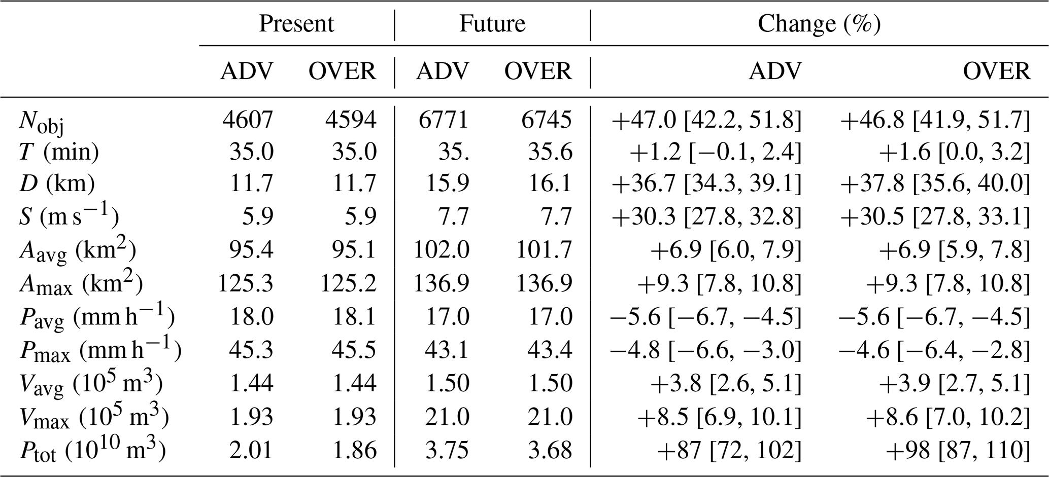
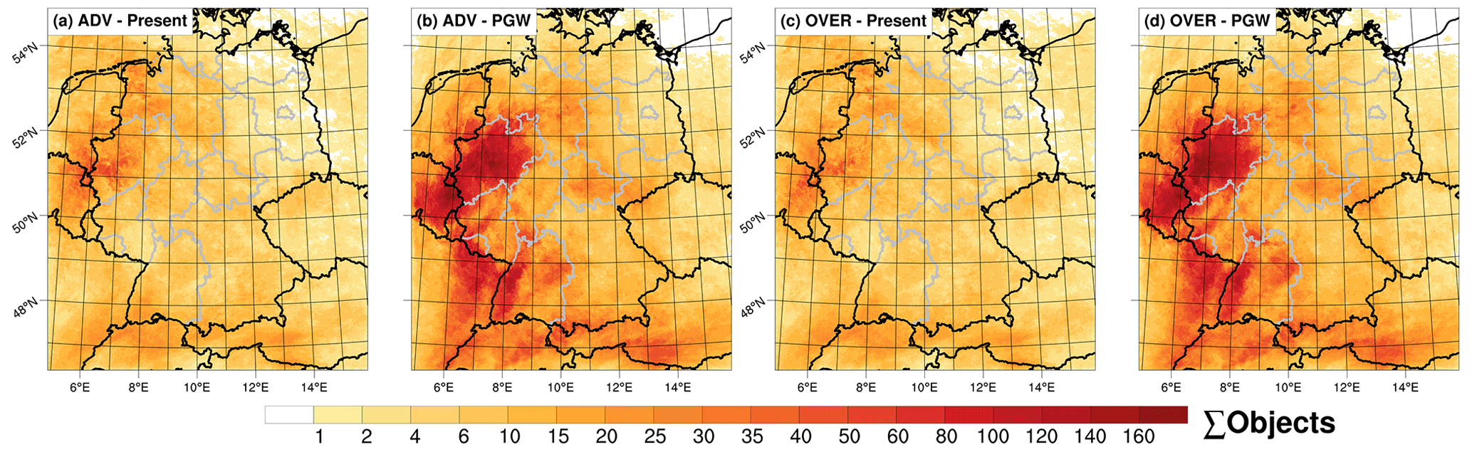
Figure 3 Total number of objects counted at each grid box for ADV in the (a) present and (b) PGW ensembles and OVER in the (c) present and (d) PGW ensembles. Results are based on the algorithms' reference setup. The analysis region is as denoted by the dashed yellow boxes in Fig. 1. Note that a higher number of objects does not necessarily correspond to higher precipitation; e.g. one large system could cause more precipitation than multiple smaller cells.

4.2 Minimum size of object (A_min)

In this subsection, we hold T_min and P_min constant at their reference values. A_min (the minimum-area threshold) is varied, with values of A_min=2ⁱ grid boxes, where i=1…6 (Fig. 4). For P_avg and P_max (the object lifetime mean and maximum precipitation intensity), the minimum object size has no significant impact on the response to warming; this is mostly true for the object lifetime too. For the remaining metrics, however, the A_min threshold has a significant impact on the resulting climate-change signal. For volume (V_avg, V_max), area (A_avg, A_max), distance travelled and average speed of the objects, the strongest climate-change signal is found for the lowest A_min, with the weakest signal for the highest A_min. For the aforementioned object characteristics, the response to warming using the lowest A_min threshold (2 grid boxes) is an order of magnitude greater than with the greatest A_min threshold (64 grid boxes). Right across the different A_min thresholds tested, statistically significant differences in the magnitude of the climate-change signal are found (as evident from the non-overlapping Goldstein–Healy CIs; see Methods). In some cases (e.g. V_avg, V_max), even the sign of the climate-change signal is different. For the number of convective objects (N_obj), the trend is reversed: the higher the A_min threshold, the stronger the climate-change signal, again with statistically significant differences. The different tracking methods are found to have no statistically significant difference in their computed climate-change signals.

An important point to note is that depending on the chosen A_min threshold, the physical interpretation for why total convective precipitation increases in the warmer climate (Fig. 7) could be different. For a small A_min, the increase in convective precipitation would appear to be driven by the area and volume of the objects increasing. For a larger A_min, on the other hand, the increase in total precipitation would appear to be driven by strong growth in the number of convective objects. That is not to say the one choice of A_min is “wrong” or another “correct” but rather to recognize that the role of object characteristics in changing total convective precipitation is conditional on how a convective object is defined and that results should be interpreted in this context. These differences are worth bearing in mind when drawing inferences about future changes in the characteristics of convective precipitation.

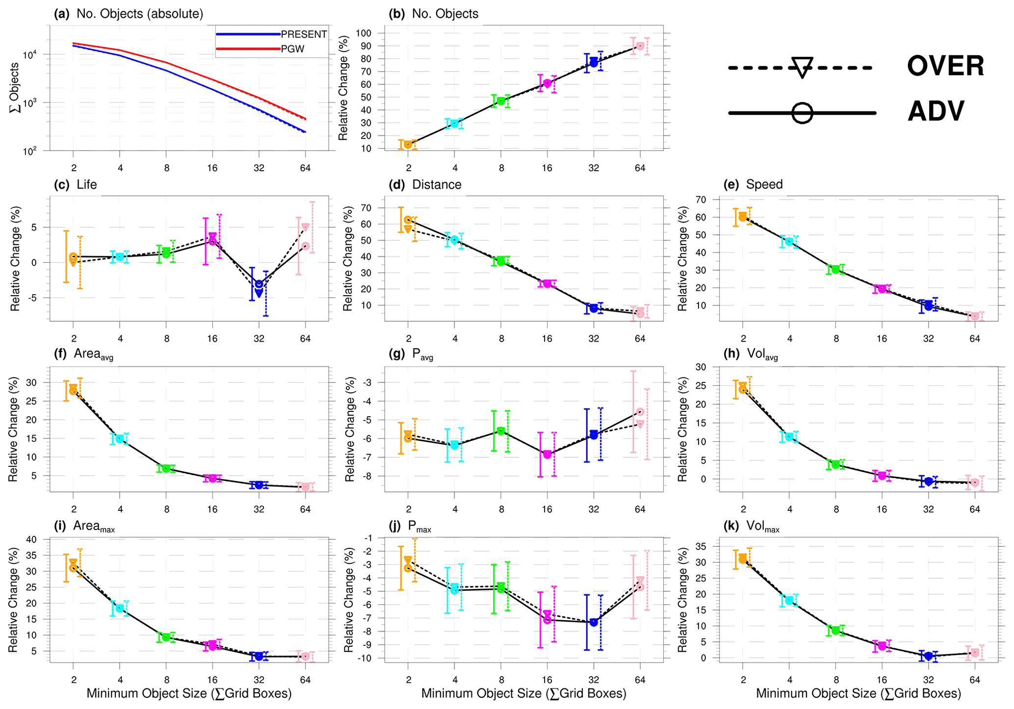
Figure 4 Climate-change signals of different object properties as a function of the object's minimum-area (A_min) criterion, for both algorithms. Change signals which are different with statistical significance at the 0.95 level can be identified based on non-overlapping CIs (Sect. 3.4), seen as vertical solid (advection) or dashed (overlap) lines. In panel (a), the numbers of objects are shown (i.e. the sample sizes). A_min is defined in terms of grid boxes, with each grid box having an area of ∼7.7 km². The A_min range thus spans approximately 15 to 493 km². The values underlying the change signals can be seen in Fig. S2.

4.3 Minimum precipitation intensity of object (P_min)

In this subsection, A_min and T_min are fixed at their reference values, while the precipitation-minimum threshold P_min is varied across values of 4.5, 6.5, 8.5, 10.5 and 12.5 mm h⁻¹ (using the equivalent 5 min rate). The choice of P_min threshold has much less of an impact on the magnitude of the climate-change signal than varying A_min. Across the sampled range of P_min thresholds, clear statistically significant differences (Fig. 5) are most evident for diagnostics which characterize the object's precipitation intensity: P_avg and P_max show a monotonic upward trend in their climate-change signal with increasing P_min; this is in contrast to varying A_min, which was shown to have no effect on the climate-change signals of P_avg and P_max. Some smaller but statistically significant differences are also seen in the object area's response to warming (A_avg, A_max; Fig. S3) and in the total number of objects. For the remaining object characteristics, the range of tested P_min thresholds produces very few significant differences in the response to warming. The speed of the objects does, however, show a clear monotonically decreasing trend (Fig. S3), suggesting that over a wider range of P_min thresholds, significant differences may emerge. As with the A_min threshold, no statistically significant differences between the tracking methods are evident.

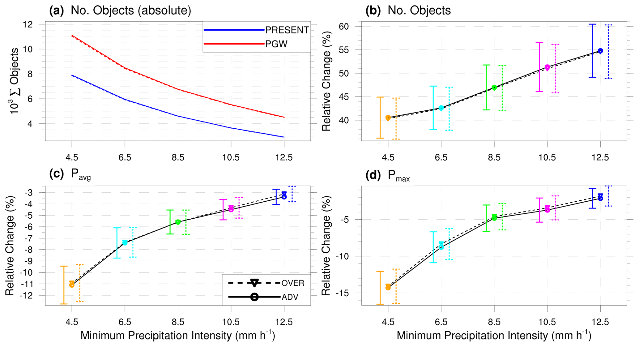
Figure 5 Climate-change signals of P_avg, P_max and N_obj as a function of the object's minimum-precipitation-intensity (P_min) criterion, for both algorithms. Change signals which are different with statistical significance at the 0.95 level can be identified based on non-overlapping CIs (Sect. 3.4), seen as vertical solid (advection) or dashed (overlap) lines. In panel (a), the numbers of objects are shown (i.e. the sample sizes). P_min is shown as the equivalent hourly rate based on 5 min intensities. The climate-change signals of the remaining object properties, as well as the values underlying them, can be seen in Figs. S3 and S4.

4.4 Minimum lifetime of object (T_min)

Here we vary the minimum-lifetime threshold T_min of the objects, while keeping P_min and A_min at their reference values (Fig. 6b and e); this is then additionally shown for the smallest and largest values of A_min (2 and 64 grid boxes; see Fig. S5 for remaining A_min values). Starting with the reference values of P_min and A_min, it is found that varying the minimum-lifetime threshold T_min has a clear and statistically significant impact on the magnitudes of the climate-change signals of the speed, distance travelled and lifetime object characteristics in both algorithms, as well as for the total number of objects. To a lesser extent, significant differences are found for the area metrics.

Looking at the smallest and greatest values of A_min, it is only the speed, distance travelled and lifetime properties which consistently display climate-change signals that are sensitive to how an object's minimum lifetime (T_min) is defined. At the lowest A_min threshold (A_min=2), all diagnostics are found to exhibit a climate-change signal with some degree of sensitivity to the magnitude of T_min, with the strongest sensitivities for the aforementioned properties, as well as the number of objects. As A_min increases, the impact of T_min on the magnitude of the climate-change signal generally decreases and is either eliminated or greatly reduced by the maximum (A_min=64 grid boxes; see also Fig. S5). A likely reason for this is that by removing smaller objects from the sample, the sample distribution of lifetimes shifts upwards, a consequence of larger objects also tending to live longer (Fig. S2b). Successively raising the T_min threshold thus has less impact on the sample statistics because in the upwards-shifted distribution the fraction of objects with lifetimes above the T_min thresholds is higher. Comparing the two tracking methods, no statistically significant differences are found between the algorithms.

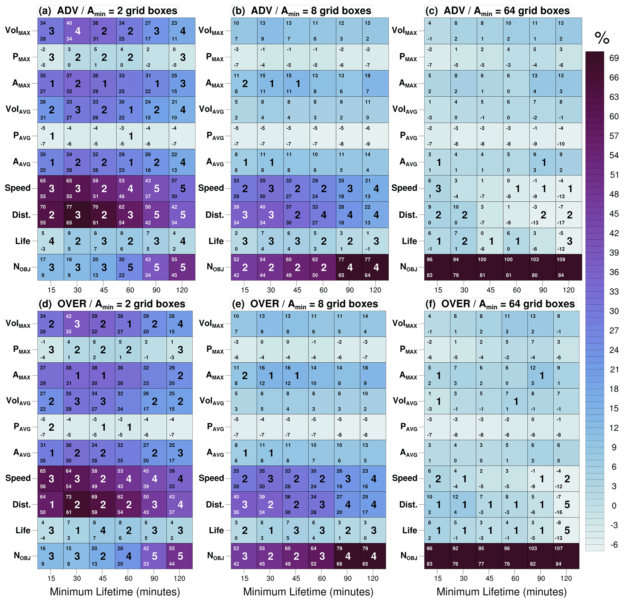
Figure 6 Climate-change signals of all object properties and N_obj, as a function of the object's minimum-lifetime (T_min) criterion, for both algorithms. A statistically significant difference in the climate-change signal against other T_min thresholds is indicated by a number in the box centre. The number denotes how many of the other T_min thresholds have a change signal whose difference is statistically significant compared to the box in question (maximum = 5). For example, for the combination (d) OVER, A_min=2, speed and T_min=15 min, the number 3 is present: this means that the climate-change signal for this combination has a statistically significant difference to three of the remaining five T_min thresholds of OVER, A_min=2 and speed. Confidence intervals, computed as in Sect. 3.4, are given in the left-hand corners of each box. There are no statistically significant differences between the algorithms. The results are shown for three values of A_min, with the remaining values of A_min found in Fig. S5 and the values underlying the change signal in Fig. S6.

4.5 Total convective precipitation

Changes in the characteristics of convective objects do not necessarily inform us about changes in total convective precipitation. An additional metric of interest in object-oriented precipitation analysis may thus be the total amount of convective precipitation attributable to the identified objects (P_tot) and how this responds to warming. By jointly varying (i) T_min and A_min and (ii) T_min and P_min, a large range of P_tot responses is found across 132 setups, with a strong P_tot increase in all cases (Fig. 7), ranging from about +70 % to +120 %, depending on the combination of the three thresholds. As with the reference setup (Sect. 4.1), considerable differences are often evident between the two algorithms, with those for OVER being typically stronger. However, due to the large range of uncertainty in the magnitude of these increases, no statistically significant differences between the tracking methods are found.

A general, though not uniform, pattern of a stronger warming response with higher T_min thresholds and lower P_min thresholds can be discerned, while no clear influence of the A_min threshold on the P_tot climate-change signal is evident. The higher increases in total precipitation with higher T_min thresholds mirror the changes seen for the number of objects as T_min increases (Fig. 6), suggesting that the latter explains differences in the climate-change signal of P_tot as T_min is varied. Higher increases in P_tot as P_min decreases, meanwhile, appear to be explained by differences in the A_avg signal as P_min is varied (Fig. S3f).

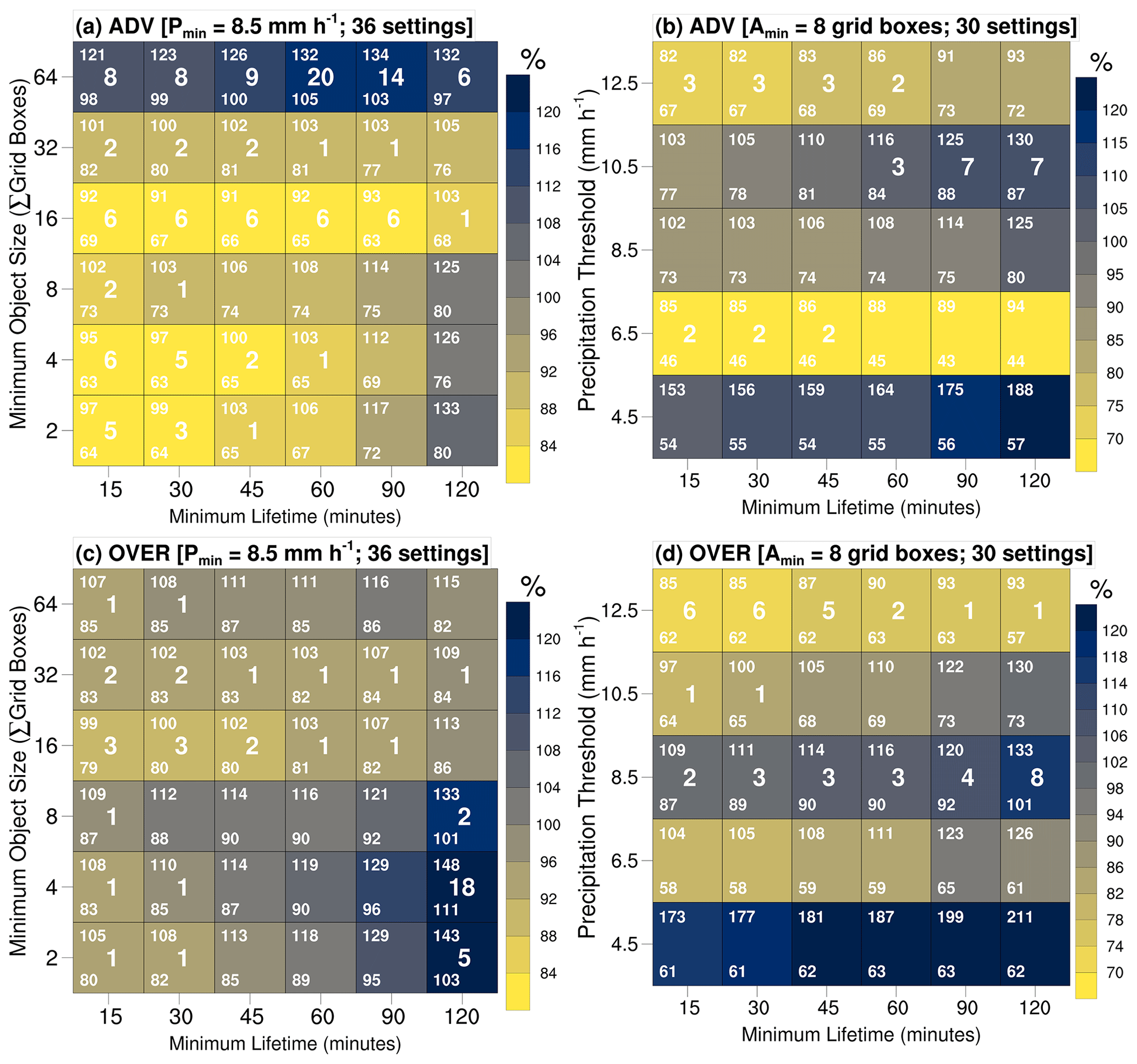
Figure 7 Change (%) in total convective precipitation in response to warming signal, for both algorithms. The change is based on the total precipitation attributable to all identified objects. In panels (a) and (c), A_min and T_min are jointly varied, with P_min at its reference value. In panels (b) and (d), P_min and T_min are jointly varied, with A_min at its reference value. Confidence intervals, computed as in Sect. 3.4, are given in the left-hand corners of each box. Statistically significant differences are denoted by a number in the middle of each square, as in Fig. 6. For example, for the case (c) OVER, A_min=2 grid boxes and T_min=120 min, the number 5 is present: this means that the change signal for this combination has a statistically significant difference to 5 of the remaining 35 configurations in (c). Note different colour-bar minima for panels (a, c) and (b, d).

4.6 Spatiotemporal resolution of precipitation data

The preceding results have shown that user-defined thresholds for identifying a convective object can affect the magnitude of the climate-change signal but that the tracking method appears to have little impact. The latter result, while encouraging, merits deeper investigation. Analysis so far has been based on 5 min precipitation sums. Here we first investigate the impact of the model data's temporal resolution by aggregating the 5 min accumulations to 15, 30, 45 and 60 min totals while keeping the reference object thresholds.

A dependence of the climate-change signal on the chosen thresholds (here, data temporal resolution) is once again found. Significant differences emerge, however, between the climate-change signals of the two tracking algorithms (Fig. 8). They are most pronounced for the distance and speed metrics. Differences tend to grow as data temporal resolution decreases, with a few exceptions. One possibility is that a disconnect between (i) where an object is predicted to advect to and (ii) the largest spatial overlap grows as temporal resolution falls: the wind field, for example, on which the advection is based is simply an hourly instantaneous value. Another factor may be a failure of smaller, fast-moving objects to overlap at successive time steps over longer accumulation periods, thus prematurely terminating tracks. Either way, both of these adverse influences would be exacerbated in a heterogeneous precipitation field, i.e. with lots of small objects rather than fewer but larger convective systems. This is supported by repeating the analysis using the lowest and highest A_min thresholds, namely 2 and 64 grid boxes (Figs. S7 and S8). At the lowest A_min, differences between the tracking algorithms grow sharply; at the highest A_min, differences disappear. This suggests that threshold choices which lead to a greater number of small objects and a more fragmented precipitation field require precipitation data with a higher temporal resolution. If this is the case, one corrective measure may be to apply a smoothing to the precipitation field for the purpose of tracking (and correspondingly reducing P_min) but use the unsmoothed field for computing the object characteristics (e.g. Müller et al., 2022).

Another influencing factor on the climate-change signal may be the spatial resolution of the precipitation data. This was tested by aggregating the model data to coarser grids, with grid boxes of dimension 2×2, 3×3, 4×4 and 5×5 native (0.025^∘) grid cells. Here, significant differences between the tracking methods were uncommon, though did appear in isolated cases (Fig. S10).

.

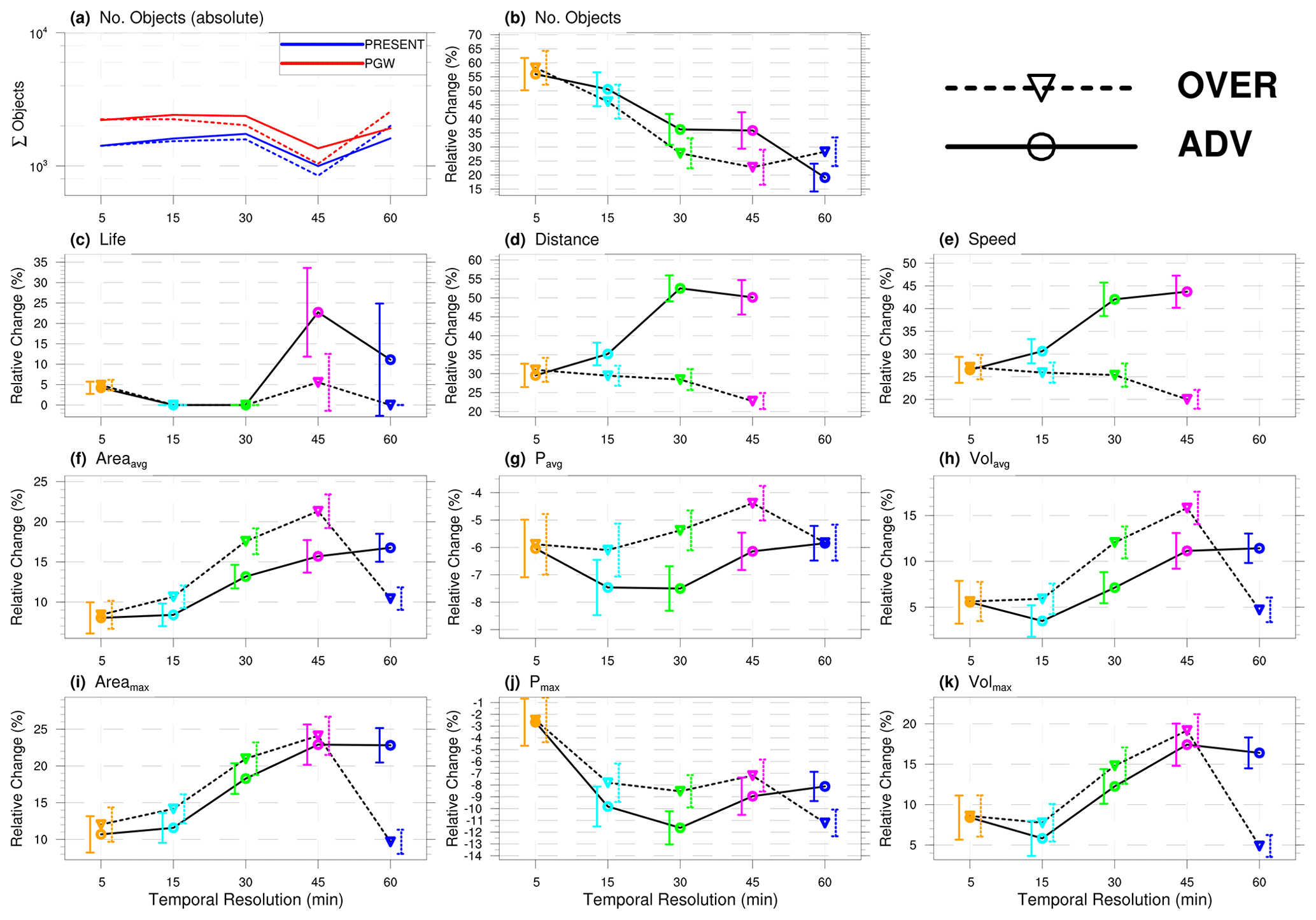
Figure 8 Climate-change signals of different object properties as a function of the precipitation data's temporal resolution, for both algorithms (A_min, P_min and T_min are kept at their reference values). Change signals which are different with statistical significance at the 0.95 level can be identified based on non-overlapping CIs (Sect. 3.4), seen as vertical solid (advection) or dashed (overlap) lines. In panel (a), the numbers of objects are shown (i.e. the sample sizes). For object properties with a median value of zero in the present climate, a percent change signal cannot be defined, hence the missing values for the 60 min distance and speed. Note that to ensure a fair comparison, only objects with a lifetime of at least 60 min are considered. Similar figures using A_min thresholds of 2 and 64 grid boxes are presented in the Supplement (Figs. S7 and S8). The values underlying the percent change are presented in Fig. S9

5 Analysis of future projections

In this section, we use our PGW experiment as a case study for exploring how Lagrangian projections might best be presented based on the lessons of Sect. 4.2 to 4.5. As it has been shown in previous sections that the choice of tracking method has no impact on our results with 5 min data resolution, we will for clarity show results for just the ADV algorithm. It should firstly be noted that our 14 d study period of high convective activity is not representative of climatological conditions: this is further underlined by contrasting our projections with those of Purr et al. (2021). The change signals in our case study are thus illustrative and only indicative for the specific synoptic conditions present during the simulation period.

In Sect. 4.2 to 4.5 it was shown that the choice of thresholds (A_min, P_min, T_min) for defining a convective object can significantly impact the magnitude of the climate-change signal. We therefore propose analysing the output of the tracking algorithm by first partitioning the data into bins delineated by different values of A_avg, P_avg or T, the metrics on which the object thresholds are based. To maximize the range covered by all bins, tracking setups with each of the three lowest thresholds – A_min=2 grid boxes, P_min=4.5 mm h⁻¹ and T_min=15 min – alongside their counterpart reference thresholds are used (Fig. 9).

Partitioning the tracks based on object mean intensity, area or lifetime reveals the potential for a given object property to exhibit quite varied warming responses. Taking mean object intensity (Fig. 9a), the climate-change signal of most object properties responds non-linearly to increasing object intensity in our case study. Maximum increases emerge for moderate-intensity objects, with minimum increases for low and high intensities. Some object properties even exhibit the potential for a change in the sign of the warming response as intensity varies: here, the change in object area flips to negative for the most intense cases. Partitioning based on object mean area (Fig. 9b), meanwhile, shows a completely different response spectrum: climate-change signals which behave asymptotically as object area increases. This behaviour suggests that the spatial homogeneity of the precipitation field is likely an important factor in the sensitivity of Lagrangian projections to object thresholds; i.e. larger area thresholds (A_min) give projections whose magnitude is less sensitive to further increases in the area threshold. Finally, the partitioning based on object lifetime (Fig. 9c) reveals yet another response spectrum of a different character to the previous: object properties which (mostly) display little sensitivity to increasing object lifetime.

The spectrum-based analysis (Fig. 9) offers insights not evident from the analyses in Sect. 4.1 to 4.5, which help to explain the mechanisms by which total precipitation increases in our case study: (1) the total number of objects increases in (almost) all cases; (2) future objects have larger areas and volumes, regardless of how long they live or how intense they are; (3) despite this, objects of all areas and lifetimes have lower mean intensities; (4) it can thus be concluded that the increase in P_tot is driven by the combined effect of more objects and an increase in the area of these objects; and (5) the increase in object volumes despite a decrease in intensity shows that the effects of more objects and higher areas are dominant over the reduction in mean object intensity, which acts in the opposing direction. While a similar interaction of these mechanisms may seem plausible for longer timescales, such a conclusion would require climate-length simulations. Of interest, perhaps, is that in agreement with the observational study of Wasko et al. (2016) and modelling experiments of Armon et al. (2022) and Caldas-Alvarez et al. (2022), the area of the most intense objects is actually found to decrease and their maximum local precipitation intensity found to increase.

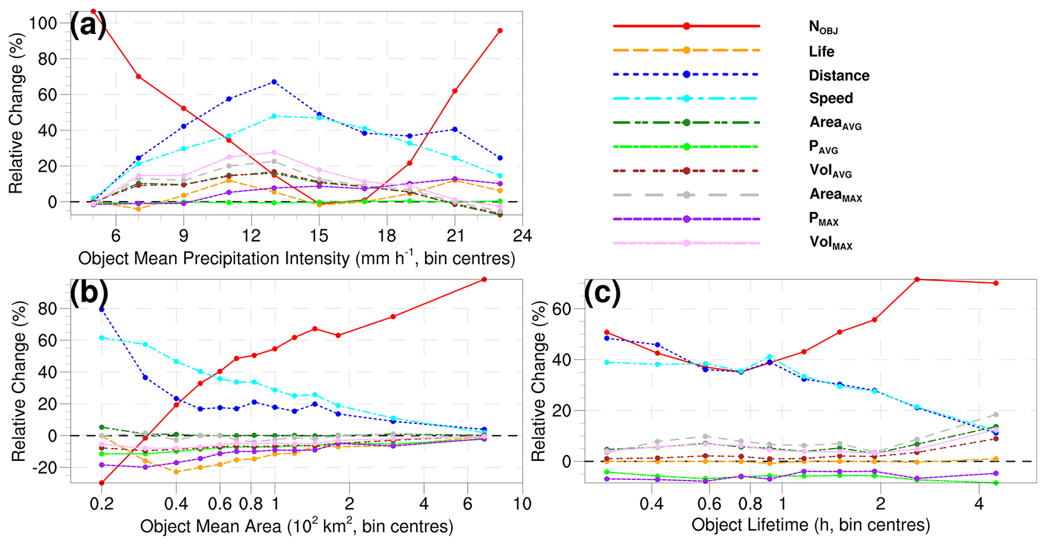
Figure 9 Ensemble mean projected change (%) in object characteristics under the RCP8.5 scenario as a function of (a) object intensity, (b) object area and (c) object lifetime. Note the logarithmic x axes in panels (b) and (c). In panels (a), (b) and (c), P_min, A_min and T_min are set at 4.5 mm h⁻¹, 2 grid boxes and 15 min, respectively, while the remaining thresholds are in each case set to their reference values. For visual clarity, results are based solely on the ADV algorithm. As in the rest of the paper, results are for median values. Each bin has a minimum of 50 data points in at least 15 of the 18 ensemble members; members with less than this total are not considered in the calculation.

6 Summary and conclusions

Aided by the growing use of kilometre-scale climate models (Lucas-Picher et al., 2021), Lagrangian methods for analysing the response of convective precipitation to climate change have become increasingly popular (e.g. Prein et al., 2017; Poujol et al., 2020a; Purr et al., 2021). This object-oriented approach is particularly useful for studying changes in the characteristics of convective cells. In our study, we have tested the sensitivity of Lagrangian projections to the choice of (i) tracking algorithm and (ii) how a convective object is defined. Two simple tracking algorithms, each representative of a common approach to Lagrangian analysis, were employed to track convective objects in convection-permitting PGW ensemble simulations, allowing for their respective climate-change signals to be compared. Furthermore, for each algorithm, the sensitivity of the climate-change signal to how a convective object is defined was examined by systematically varying the threshold criteria for identifying a convective object, namely: minimum size (A_min), intensity (P_min) and lifetime (T_min). In total, 132 configurations were tested. Our PGW simulations encompassed a 14 d period with elevated levels of both strongly and weakly forced convection (Sect. 2), offering a diverse representation of convective objects against which the different algorithms and configurations could be tested.

Our first main result is that – as long as the precipitation data are of sufficiently high temporal resolution – the tracking method appears to have no significant impact on how the properties of convective objects or the total number of convective objects respond to climate change. Area thresholds which permit a higher number of small objects, thus creating a less homogenous precipitation field, were shown to necessitate input data with a higher temporal resolution; otherwise the climate-change signals diverge. Adjusting for this caveat, the representative advection- and overlap-based algorithms which we implemented produce very similar climate-change signals for all object properties, with no statistically significant differences found. Additional tests of this conclusion using a set of climate-length simulations, those used in Meredith et al. (2019), show that the insensitivity of the climate-change signal to the tracking method remains consistent (Fig. S11 and accompanying discussion). This conclusion likely extends to the pattern-matching approach (e.g. Einfalt et al., 1990): a precipitation field with larger objects and, hence, more spatial homogeneity is less likely to see large changes in structure over short temporal scales.

Our second main result is that, unlike the tracking algorithm, the definition of what constitutes a convective object has a potentially large impact on the climate-change signal for all object properties, as well as for changes in the total number of objects. The thresholds of minimum precipitation intensity (P_min), minimum size (A_min) and minimum lifetime (T_min) for identifying a convective object were all found to be relevant. How the climate-change signal responds to varying these thresholds was found to depend on the object property under investigation. For example, the minimum object size had no significant impact on changes in the object's precipitation intensity but did lead to different climate-change signals for changes in the total number of objects, as well as changes in object properties like the integrated precipitation volume and distance travelled. Similarly, the threshold for minimum intensity affected the climate-change signal of object intensity but was not relevant for e.g. changes in the object volume. Changes in total convective precipitation were also sensitive to how an object is defined. As discussed in the Introduction, the definition of what constitutes a convective object shows considerable variance in the literature. An open question in climate-change research is whether the spatial extent of convective storms will increase or decrease with warming (Fowler et al., 2021). Our results suggest that, at least in some regions, the answer may be dependent on how a convective storm is defined.

The results for higher quantiles are generally as expected based on those described above for the median. An exception is for the climate-change signal of precipitation intensity as P_min increases, which sees a levelling off at higher thresholds. Otherwise, the main difference is that, in many cases, the uncertainty in the climate-change signal grows so that the number of statistically significant differences based on different object definitions reduces (Figs. S13–S15 and accompanying discussion). Uncertainty due to the higher quantiles would be expected to decrease with a larger sample of convective objects, e.g. from longer, climate-length simulations.

To reduce the sensitivity of Lagrangian-based projections to how an object is defined, we suggest performing spectrum-based analysis by first e.g. binning the data based on object area, intensity or lifetime before computing the desired statistic within each range of interest. Using this approach, a more comprehensive picture of the physical mechanisms underlying future changes in precipitation can also be obtained (Sect. 5). Results will, however, still be lower-bounded by the object areas, intensities and lifetimes chosen as threshold criteria. Lowering the thresholds will thus expand the range of the results. Here, the lower limits are dictated by computing resources and the thresholds relevant for the experiment.

Our results hint that the sensitivity of the climate-change signal to how an object is defined may, for certain (not all) object properties, decline as object size increases (Figs. 4, 6, 9b, S4). Were this the case, then studies focused on larger precipitation systems (e.g. Nissen and Ulbrich, 2017; Prein et al., 2017) could be expected to lead to higher certainty; as shown in Sect. 4.6, larger objects also eliminate divergence between the tracking methods stemming from the input data's temporal resolution. This finding, however, cannot automatically be extrapolated to other weather situations or studies at climate timescales and, thus, requires further investigation. It is similarly true that the sensitivities found for our test period would not necessarily be the same sensitivities found in other studies, as our experiment encompasses a specific period, region and climate-change profile. What we have demonstrated is the principle that in Lagrangian analyses of convective cells, the climate-change signal of different object properties can be sensitive to the conditions set for identifying an object. This dependency also has consequences for diagnosing the physical mechanisms underlying future changes in total convective precipitation. The relative importance of specific object properties in interpreting changes in total convective precipitation will not remain constant if these properties' climate-change signals respond differently to changes in the criteria for detecting an object. As such, analysing Lagrangian projections by first partitioning the data based on specific object properties (e.g. intensity, area, lifetime) can also clarify the underlying mechanisms by which future precipitation changes.

For researchers studying future changes in convective precipitation using Lagrangian methods, the first message is that, amongst the standard approaches, the choice of tracking algorithm will have little impact on the results as long as the precipitation data are not of too-low temporal resolution (“too-low” being dependent on the area criterion for defining an object). The second message is that the minimum thresholds for what constitutes a convective object should be carefully chosen based on what is most appropriate for (1) the study region and (2) the aims of the study. When making such threshold choices, the performance of the model in the present climate – e.g. by evaluating against radar (Caine et al., 2013; Raupach et al., 2021) – should also be factored in. Alongside this, the change signal across a range of object intensities, areas and lifetimes should be explored (see Fig. 9). To conclude, Lagrangian analysis is an important technique for studying future changes in precipitation. To make the best use of this approach, the uncertainties in the climate-change signal associated with how a convective object is defined should be examined wherever possible.