the Creative Commons Attribution 4.0 License.
the Creative Commons Attribution 4.0 License.
 | 03 Feb 2023
Parallelized domain decomposition for multi-dimensional Lagrangian random walk mass-transfer particle tracking schemes
Lucas Schauer
Michael J. Schmidt
Nicholas B. Engdahl
Stephen D. Pankavich
David A. Benson
Diogo Bolster
Lagrangian particle tracking schemes allow a wide range of flow and transport processes to be simulated accurately, but a major challenge is numerically implementing the inter-particle interactions in an efficient manner. This article develops a multi-dimensional, parallelized domain decomposition (DDC) strategy for mass-transfer particle tracking (MTPT) methods in which particles exchange mass dynamically. We show that this can be efficiently parallelized by employing large numbers of CPU cores to accelerate run times. In order to validate the approach and our theoretical predictions we focus our efforts on a well-known benchmark problem with pure diffusion, where analytical solutions in any number of dimensions are well established. In this work, we investigate different procedures for “tiling” the domain in two and three dimensions (2-D and 3-D), as this type of formal DDC construction is currently limited to 1-D. An optimal tiling is prescribed based on physical problem parameters and the number of available CPU cores, as each tiling provides distinct results in both accuracy and run time. We further extend the most efficient technique to 3-D for comparison, leading to an analytical discussion of the effect of dimensionality on strategies for implementing DDC schemes. Increasing computational resources (cores) within the DDC method produces a trade-off between inter-node communication and on-node work. For an optimally subdivided diffusion problem, the 2-D parallelized algorithm achieves nearly perfect linear speedup in comparison with the serial run-up to around 2700 cores, reducing a 5 h simulation to 8 s, while the 3-D algorithm maintains appreciable speedup up to 1700 cores.
- Article
(5429 KB) - Full-text XML
- BibTeX
- EndNote


Numerical models are used to represent physical problems that may be difficult to observe directly (such as groundwater flow) or that may be tedious, expensive, or even impossible to currently study via other methods. In the context of groundwater flow, for example, these models allow us to portray transport in heterogeneous media and bio-chemical species interaction, which are imperative to understanding a hydrologic system's development (e.g., Dentz et al., 2011; Perzan et al., 2021; Steefel et al., 2015; Scheibe et al., 2015; Tompson et al., 1998; Schmidt et al., 2020b; Li et al., 2017; Valocchi et al., 2019). Since geological problems frequently require attention to many separate, yet simultaneous processes and corresponding physical properties, such as local mean velocity (advection), velocity variability (dispersion), mixing (e.g., dilution), and chemical reaction, we must apply rigorous methods to ensure proper simulation of these processes. Recent studies (e.g., Benson et al., 2017; Bolster et al., 2016; Sole-Mari et al., 2020) have compared classical Eulerian (e.g., finite-difference or finite-element) solvers to newer Lagrangian methods and have shown the relative advantages of the latter. Therefore, in this paper we explore several approaches to parallelize a Lagrangian method that facilitate the simulation of the complex nature of these problems. Given that all of the complex processes noted above must ultimately be incorporated and that this is the first rigorous study of this kind, we focus on well-established and relatively simple benchmark problems with analytical solutions to derive a rigorous approach to this parallelization.
Lagrangian methods for simulating reactive transport continue to evolve, providing both increased accuracy and accelerated efficiency over their Eulerian counterparts by eliminating numerical dispersion (see Salamon et al., 2006) and allowing direct simulation of all subgrid processes (Benson et al., 2017; Ding et al., 2017). Simulation of advection and dispersion (without reaction) in hydrogeological problems began with the Lagrangian random walk particle tracking (RWPT) algorithm that subjects an ensemble of particles to a combination of velocity and diffusion processes (LaBolle et al., 1996; Salamon et al., 2006). Initially, chemical reactions were added in any numerical time step by mapping particle masses to concentrations via averaging over Eulerian volumes, then applying reaction rate equations, and finally mapping concentrations back to particle masses for RWPT (Tompson and Dougherty, 1988). This method clearly assumes perfect mixing within each Eulerian volume because subgrid mass and concentration perturbations are smoothed (averaged) prior to reaction. The subsequent over-mixing was recognized to induce a scale-dependent apparent reaction rate that depended on the Eulerian discretization (Molz and Widdowson, 1988; Dentz et al., 2011), thus eliminating some of the primary benefits of the Lagrangian approach. In response, a method that would allow reactions directly between particles was devised and implemented (Benson and Meerschaert, 2008).
Early efforts to directly simulate bimolecular reactions with RWPT algorithms (Benson and Meerschaert, 2008; Paster et al., 2014) were originally founded on a birth–death process that calculated two probabilities: one for particle-particle collocation and a second for reaction and potential transformation or removal given collocation (i.e., particles that do not collocate cannot react, thus preserving incomplete mixing). The next generation of these methods featured a newer particle-number-conserving reaction scheme. This concept, introduced by Bolster et al. (2016) and later generalized (Benson and Bolster, 2016; Schmidt et al., 2019; Sole-Mari et al., 2019), employs kernel-weighted transfers for moving mass between particles, where the weights are equivalent to the abovementioned collision probabilities under certain modeling choices. These algorithms preserve the total particle count, and we refer to them as mass-transfer particle tracking (MTPT) schemes. These particle-conserving schemes address low-concentration resolution issues that arise spatially when using particle-killing techniques (Paster et al., 2013; Benson et al., 2017). Furthermore, MTPT algorithms provide a realistic representation of solute transport with their ability to separate mixing and spreading processes (Benson et al., 2019). Specifically, spreading processes due to small-scale differential advection may be simulated with standard random walk techniques (LaBolle et al., 1996), and true mixing-type diffusive processes may be simulated by mass transfers between particles. MTPT techniques are also ideally suited to, and provide increased accuracy for, complex systems with multiple reactions (Sole-Mari et al., 2017; Engdahl et al., 2017; Benson and Bolster, 2016; Schmidt et al., 2020b), but they are computationally expensive because nearby particles must communicate. This notion of nearness is discussed in detail in Sect. 3.
The objective of this study is to develop efficient, multi-dimensional parallelization schemes for MTPT-based reactive transport schemes. We conduct formal analyses to provide cost benchmarks and to predict computational speedup for the MTPT algorithm, both of which to date were only loosely explored in the 1-D case (Engdahl et al., 2019). Herein, we focus on an implementation that uses a multi-CPU environment that sends information between CPUs via Message Passing Interface (MPI) directives within Fortran code. In particular, we focus on the relative computational costs of the inter-particle mass transfer versus message passing algorithms because the relative costs of either depend upon the manner in which the computational domain is split among cores. These mass-transfer methods may be directly compared to smoothed-particle hydrodynamics (SPH) methods and are equivalent when a Gaussian kernel is chosen to govern the mass transfers (Sole-Mari et al., 2019). Specifically, this work shares similarities with previous investigations of parallelized SPH methods (Crespo et al., 2011; Gomez-Gesteira et al., 2012; Xia and Liang, 2016; Morvillo et al., 2021) but is novel as it tackles nuances that arise specifically for MTPT approaches. A substantial difference within this work is that the kernels are based on the local physics of diffusion rather than a user-defined function chosen for attractive numerical qualities like compact support or controllable smoothness. This adherence to local physics allows for increased modeling fidelity, including the simulation of diffusion across material discontinuities or between immobile (solid) and mobile (fluid) species (Schmidt et al., 2020a, 2019). In general, the parallelization of particle methods depends on assigning groups of particles to different processing units. Multi-dimensional domains present many options on how best to decompose the entire computational domain in an attempt to efficiently use available computing resources. Along these lines, we compare two different domain decomposition (DDC) approaches. In the one-dimensional case (Engdahl et al., 2019), the specified domain is partitioned into smaller subdomains so that each core is only responsible for updating the particles' information inside of a fixed region, though information from particles in nearby subdomains must be used. Hence, the first two-dimensional method we consider is a naive extension from the existing one-dimensional technique (Engdahl et al., 2019) that decomposes the domain into vertical slices along the x axis of the xy plane. This method is attractive for its computational simplicity but limits speedup for large numbers of cores (see Sect. 7). Our second method decomposes the domain into a “checkerboard” consisting of subdomains that are as close to squares (or cubes) as is possible given the number of cores available. RWPT simulations without mixing often require virtually no communication across subdomain boundaries because all particles act independently in the model. However, MTPT techniques require constant communication along local subdomain boundaries at each time step, which leads to challenges in how best to accelerate these simulations without compromising the quality of solutions. This novel, multi-dimensional extension of parallelized DDC techniques for the MTPT algorithm will now allow for the simulation of realistic, computationally expensive systems in seconds to minutes rather than hours to days. Further, based on given simulation parameters, we provide formal run time prediction analysis that was only hypothesized in previous work and will allow future users to optimize parallelization prior to executing simulations. This paper rigorously explores the benefits of our parallelized DDC method while providing guidelines and cautions for efficient use of the algorithm.
An equation for a chemically conservative, single component system experiencing local mean velocity and Fickian diffusion-like dispersion is
where C(x,t) [mol L−d] is the concentration of a quantity of interest, v(x,t) [LT−1] is a velocity field, and D(v) [L2T−1] is a given diffusion tensor. Advection–diffusion equations of this form arise within a variety of applied disciplines relating to fluid dynamics (Bear, 1972; Tennekes and Lumley, 1972; Gelhar et al., 1979; Bear, 1961; Aris, 1956; Taylor, 1953). Depending on the physical application under study, various forms of the diffusion tensor may result. Often, it can be separated into two differing components, with one representing mixing between nearby regions of differing concentrations and the other representing spreading from the underlying flow (Tennekes and Lumley, 1972; Gelhar et al., 1979; Benson et al., 2019). This decomposition provides a general splitting of the tensor into
Lagrangian numerical methods, such as those developed herein, can then be used to separate the simulation of these processes into mass-transfer algorithms that capture the mixing inherent to the system and random walk methods that represent the spreading component (see, e.g., Ding et al., 2017; Benson et al., 2019). As our focus here is mainly driven by the novel implementation of diffusive processes in MTPT algorithms, we will for now assume a purely diffusive system so that v(x)=0. This assumption results in an isotropic diffusion tensor that reduces to
where Id is the d×d identity matrix. The remaining scalar diffusion coefficient can also be separated into mixing and spreading components, according to
Despite the assumption of zero advection, we simulate spreading via random walks as an eventual necessity for moving particles within our DDC scheme. Stationary particles do not provide computational complexity for the mass-transfer algorithm as distances between particles remain constant.
2.1 Initial conditions and analytic solution
We define a general and well-established benchmark test problem to facilitate the analysis of speedup and computational efficiency. Based on the chosen tiling method, the global domain is subdivided into equi-sized subdomains, and each core knows its own local, non-overlapping domain limits. The particles are then load balanced between the cores and randomly scattered within the local domain limits. To represent the initial mass distribution, we use a Heaviside function in an Ld-sized domain, which assigns all particles with position with mass M=1 and assigns no mass to particles with position (i.e., a heaviside step function initial condition). This initial condition will allow us to assess the accuracy of simulations as, for an infinite domain (simulated processes occur away from boundaries for all time), it admits an exact analytical solution
where and t is the elapsed time of the simulation. The existence of an analytical solution is beneficial to our ability to rigorously test our proposed schemes. We compare simulated results to this solution using the root-mean-squared error (RMSE). Note that all dimensioned quantities are unitless for the analysis we conduct and all references to run times are measured in CPU wall clock time.
2.2 Simulation parameters
Unless otherwise stated, all 2-D simulations will be conducted with the following computational parameters: the L×L domain is fixed with L=1000; the time step is fixed to Δt=0.1; the number of particles is N=107; and the diffusion constant is chosen to be D=1. The total time to be simulated is fixed as T=10, which results in 100 time steps during each simulation.
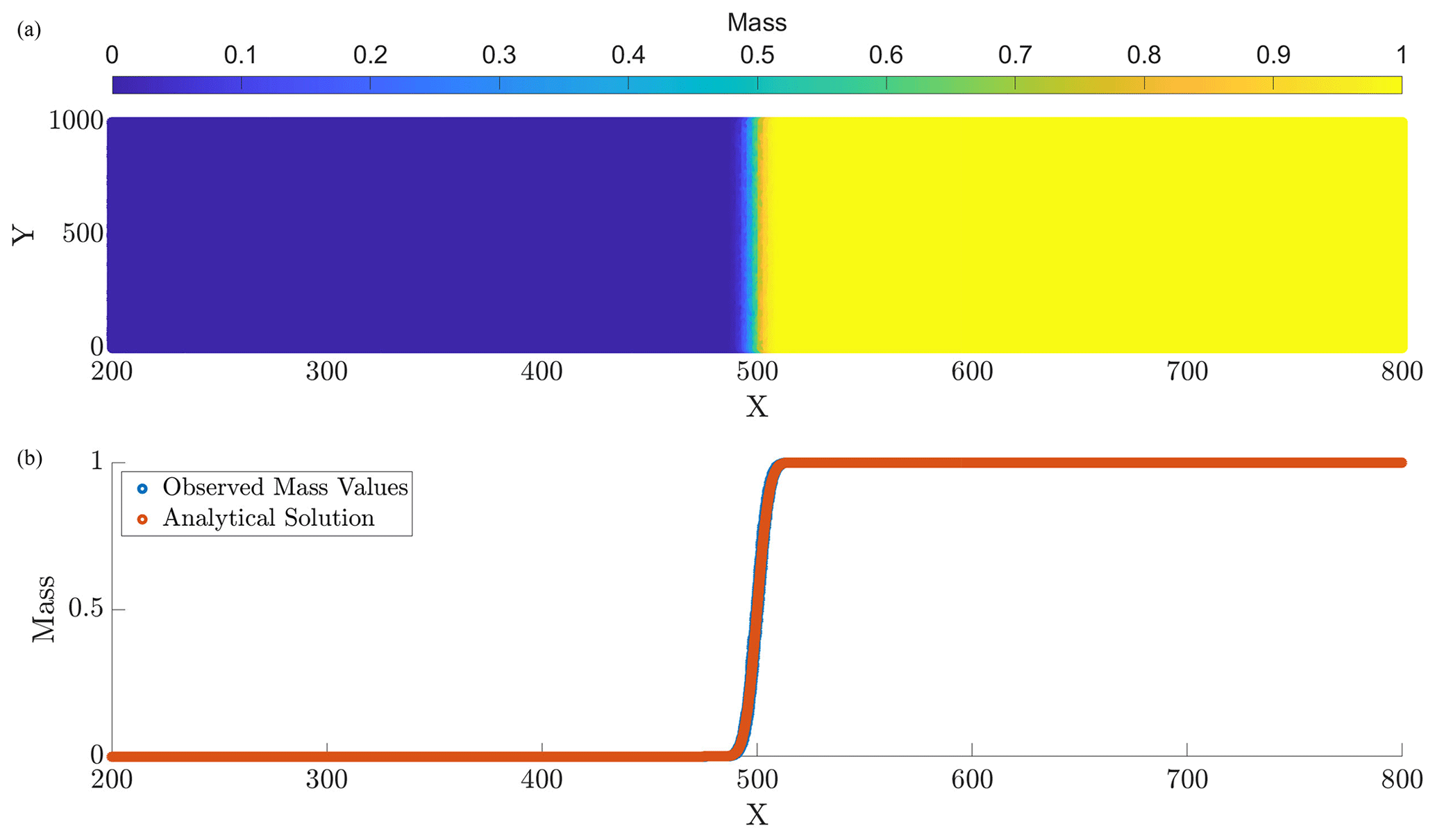
Figure 1Panel (a) displays the computed particle masses at final simulation time T=10, and panel (b) provides a computed vs. analytical solution comparison at the corresponding time. The parameters for this run are N=107, Δt=0.1, and D=1.
We choose parameters in an attempt to construct computationally intense problems that do not exceed available memory. A roofline analysis plot (NERSC, 2018; Williams et al., 2009; Ofenbeck et al., 2014; Sun et al., 2020) is provided in Appendix A to demonstrate that an optimized baseline was used for the speedup results we present. Further, we intend to retain similar computational cost across dimensionality. Hence, all 3-D simulations will be conducted with the same diffusion constant and time step size, but they will be in an L3 domain with L=100 and with a number of particles . In general, we will always use a Δt that satisfies the optimality condition
formulated in Schmidt et al. (2022), in which β is a kernel bandwidth parameter described in Sect. 3.
2.3 Hardware configuration
The simulations in this paper were performed on a heterogeneous high-performance computing (HPC) cluster called Mio, which is housed at the Colorado School of Mines. Each node in the cluster contains 8–24 cores, with clock speeds ranging from 2.50 to 3.06 GHz and memory capacity ranging from 24 to 64 GB. Mio uses a network of Infiniband switches to prevent performance degradation in multi-node simulations. We use the compiler gfortran with optimization level 3, and the results we present are averaged over an ensemble of five simulations to reduce noise that is largely attributable to the heterogeneous computing architecture.
The MTPT method simulates diffusion by weighted transfers of mass between nearby particles. These weights are defined by the relative proximity of particles that is determined by constructing and searching a k-D tree (Bentley, 1975). Based on these weights, a sparse transfer matrix is created that governs the mass updates for each particle at a given time step. As previously noted (Schmidt et al., 2018), particle tracking methods allow the dispersive process to be simulated in two distinct ways by allocating a specific proportion to mass transfer and the remaining portion to random walks. Given the diffusion coefficient D, we introduce such that
and
We choose κ=0.5 to give equal weight to the mixing and spreading in simulations. Within each time step, the particles first take a random walk in a radial direction, the size of which is based on the value of DRW. Thus, we update the particle positions via the first-order expansion
where ξi [TL−1] is a standard normal Gaussian random variable. We enforce zero-flux boundary conditions, implemented as a perfect elastic collision/reflection when particles random-walk outside of the domain. We define a search radius, ψ, that is used in the k-D tree algorithm given by
where is the standard deviation of the mass-transfer kernel, Δt is the size of the time step, DMT is the mass-transfer portion of the diffusion coefficient, and λ is a user-defined parameter that determines the radius of the search. We choose a commonly employed value of λ=6, as this will capture more than 99.9 % of the relevant particle interactions; however, using smaller values of λ can marginally decrease run time at the expense of accuracy. Using the neighbor list provided by the k-D tree, a sparse weight matrix is constructed that will transfer mass amongst particles based on their proximity. Since particles are moving via random walks, the neighbor list and corresponding separation distances will change at each time step, requiring a new k-D tree structure and sparse weight matrix within each subdomain. The mass-transfer kernel we use is given by
Here, β>0 is a tuning parameter that encodes the mass-transfer kernel bandwidth , and we choose β=1 hereafter. Recalling DMT=DMTI and substituting for the kernel bandwidth , we can simplify the formula in Eq. (11) to arrive at
Next, we denote
for each and normalize the mass-transfer (MT) kernel to ensure conservation of mass (Sole-Mari et al., 2019; Herrera et al., 2009; Schmidt et al., 2017). This produces the weight matrix W with entries
which is used in the mass-transfer step (15). The algorithm updates particle masses, Mi(t), via the first-order approximation
where
is the change in mass for a particular particle during a time step. This can also be represented as a matrix-vector formulation by computing
where M is the vector of particle masses, and then updating the particle masses at the next time step via the vector addition
In practice, imposing the cut-off distance ψ from Eq. (10) further implies that W is sparse and allows us to use a sparse forward matrix solver to efficiently compute the change in mass. Finally, the algorithm can convert masses into concentrations for comparison with the analytic solution using
in d dimensions with an Ld-sized simulation domain.
With the foundation of the algorithm established, we focus on comparing alternative tiling strategies within the domain decomposition method and their subsequent performance.
4.1 Slices method
The first approach extends the 1-D technique by slicing the 2-D domain along a single dimension, depending on how many cores are available for use. For example, depending on the number of computational cores allocated for a simulation, we define the width of each region as
where NΩ is the number of subdomains. In addition, we impose the condition that NΩ is equal to the number of allocated computational cores. So, the region of responsibility corresponding to the first core will consist of all particles with x values in the range [xmin,Δx), and the next core will be responsible for all particles with x values in the interval [Δx,2Δx). This pattern continues through the domain with the final core covering the last region of . Each of these slices covers the entirety of the domain in the y direction, so that each core's domain becomes thinner as the number of cores increases. A graphical example of the slices method decomposition is shown in Fig. 2a.
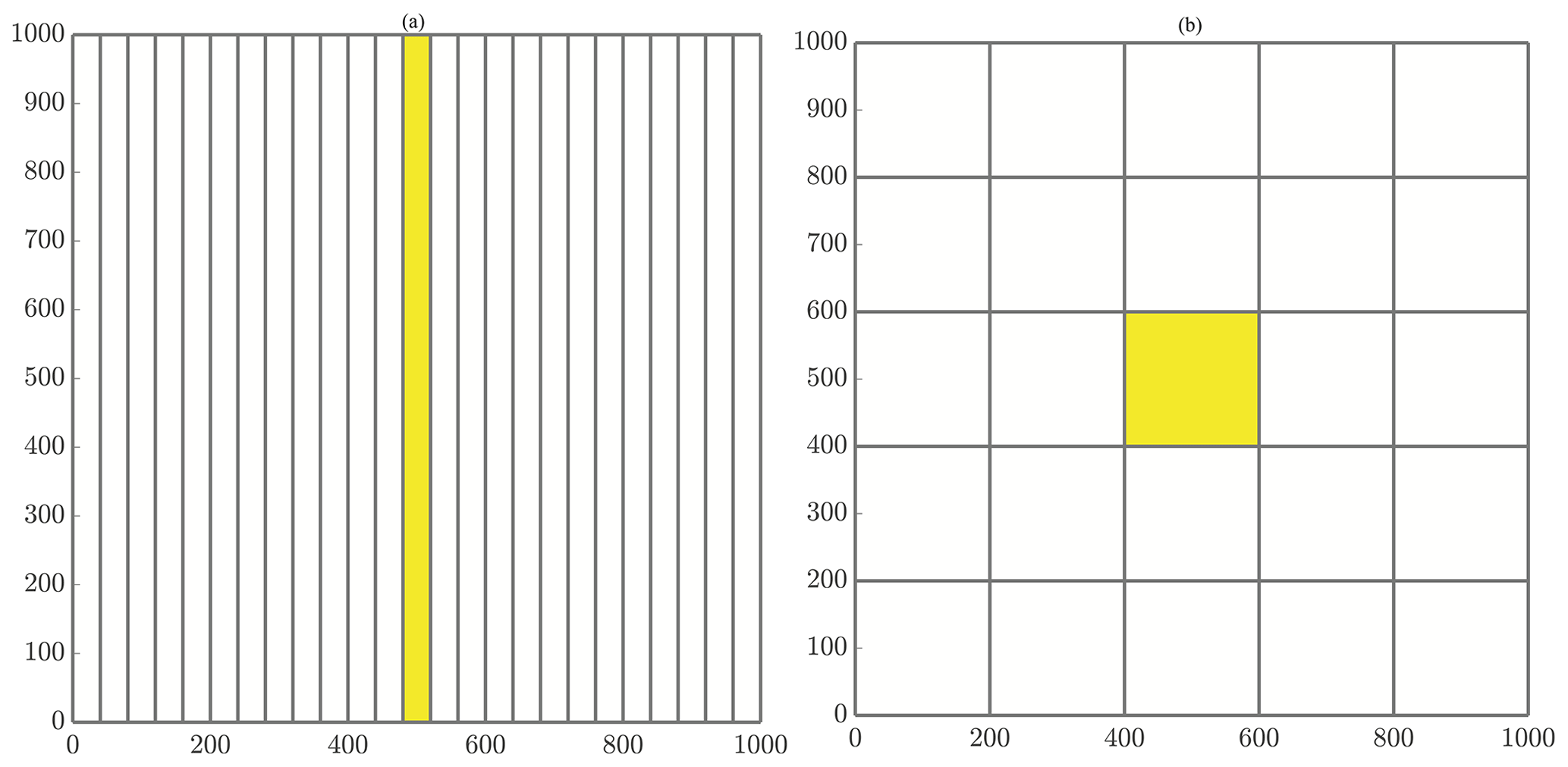
Figure 2General schematics of (a) slices and (b) checkerboard domain decompositions. (a) Decomposing the domain with 25 cores using the slices method. Figure 4a displays an enlarged slices domain with a description of ghost particle movement as well. (b) Decomposing the domain with 25 cores using the checkerboard method. Figure 4b displays an enlarged checkerboard domain with a description of ghost particle movement as well.
4.2 Checkerboard method
In addition to the slices method, we consider decomposing the domain in a tiled or checkerboard manner. Given a W×H domain (without loss of generality, we assume W≥H), we define to be the aspect ratio. Then, choosing NΩ subdomains (cores) we determine a pair of integer factors, with f1≤f2, whose ratio most closely resembles that of the full domain, i.e., f1f2=NΩ such that
for any other pair . Then, we decompose the domain by creating rectangular boxes in the horizontal and vertical directions to most closely resemble squares in 2-D or cubes in 3-D. If the full domain is taller than it is wide, then f2 is selected as the number of boxes in the vertical direction. Alternatively, if the domain is wider than it is tall, we choose f1 for the vertical decomposition. If we assume that W≥H as above, then the grid box dimensions are selected to be
and
With this, we have defined a grid of subregions that cover the domain, spanning f2 boxes wide and f1 boxes tall to use all of the allocated computational resources. Assuming NΩ is not a prime number, this method results in a tiling decomposition as in Fig. 2b. Note that using a prime number of cores reverts the checkerboard method to the slices method.
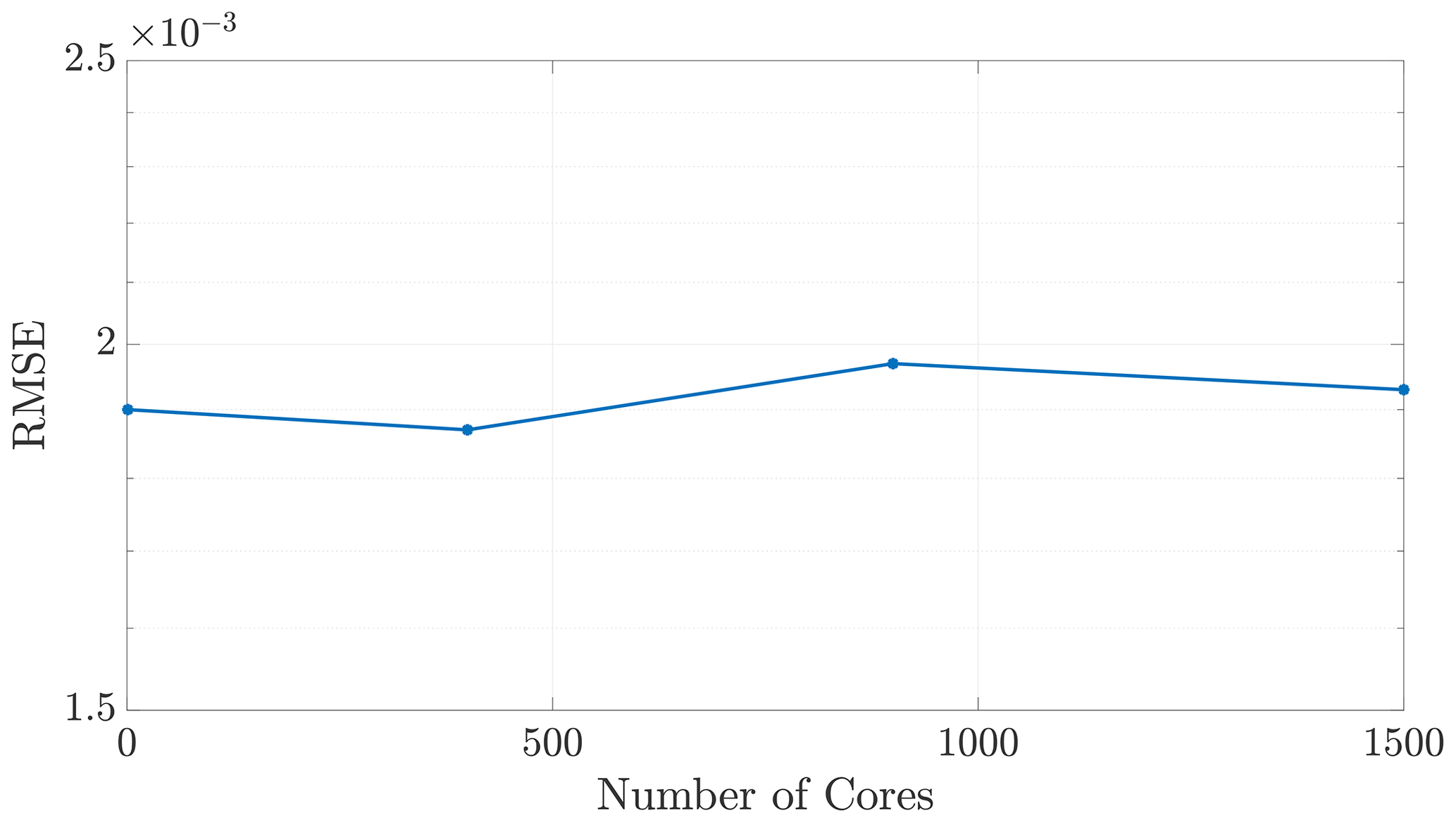
Figure 3The algorithm does not incur noteworthy changes in error, as a function of NΩ for the 2-D checkerboard DDC method considered here, nor in any of the simulations that were performed.
In MTPT algorithms, nearby particles must interact with each other. Specifically, a particle will exchange mass with all nearby particles within the search radius in Eq. (10). Our method of applying domain decomposition results in subdomains that do not share memory with neighboring regions. If a particle is near a local subdomain boundary, it will require information from particles that are near that same boundary in neighboring subdomains. Thus, each core requires information from particles in a buffer region just outside the core's boundaries, and because of random walks, the particles that lie within this buffer region must be determined at each time step. The size of this buffer zone is defined by the search distance in Eq. (10). The particles inside these buffers are called “ghost” particles and their information is sent to neighboring subdomains' memory using MPI. Because each local subdomain receives all particle masses within a ψ-sized surrounding buffer of the boundary at each time step, the method is equivalent to the NΩ=1 case after constructing the k-D tree on each subdomain, resulting in indistinguishable nearest-neighbor lists. Although ghost particles contribute to mass-transfer computations, the masses of the original particles, to which the ghost particles correspond, are not altered via computations on domains in which they do not reside. Thus, we ensure an accurate, explicit solve for only the particles residing within each local subdomain during each time step.
The process we describe here differs depending on the decomposition method. For example, the slices method gives nearby neighbors only to the left and to the right (Fig. 4a). On the other hand, the checkerboard method gives nearby neighbors in eight directions.

Figure 4All particles within a buffer width of ψ from the boundary of a subdomain (blue) are sent to the left and to the right for reaction in the slices method (a), whereas they are sent to eight neighboring regions in the checkerboard method (b). Note that the red lines depict subdomain boundaries, and the black arrows indicate the outward send of ghost particles to neighbors. Also, note that the tails of the black arrows begin within the blue buffer region. Ghost pad size is exaggerated for demonstration.
The communication portion of the algorithm becomes more complicated as spatial dimensions increase. In 3-D, we decompose the domain using a similar method to prescribe a tiling as in 2-D, but the extra sends and receives to nearby cores significantly increase. For example, the 2-D algorithm must pass information to eight nearby cores, whereas the 3-D algorithm must pass information to 26 nearby cores – eight neighboring cores on the current plane and nine neighboring cores on the planes above and below.
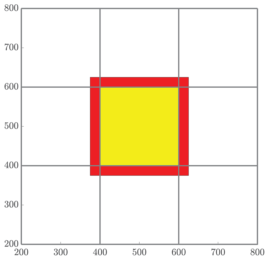
Figure 5The red band represents all particles that will be received by the local subdomain (yellow) from neighboring regions for mass transfer. The number NS quantifies the number of particles that are involved in the MT step of the algorithm, which is the combination of all particles whose positions are in either the red or yellow region.
6.1 Mass-transfer cost
In this section, we characterize and predict the amount of work being performed within each of portion of the algorithm. The general discussion of work and cost here refer to the run times required within distinct steps of the algorithm. We profile the code that implements the MTPT algorithm using the built-in, Unix-based profiling tool gprof (Graham et al., 2004) that returns core-averaged run times for all parent and child routines. The two main steps upon which we focus are the communication step and the MT step. For each subdomain, the communication step determines which particles need to be sent (and where they should be sent) and then broadcasts them to their correct nearby neighbors. The MT step carries out the interaction process described in Sect. 3 using all of the particles in a subdomain and the associated ghost particles, the latter of which are not updated within this process. As these two processes are the most expensive components of the algorithm, they will allow us to project work expectations onto problems with different dimensions and parameters.
We begin with an analysis of the MT work. First, in the interest of tractability, we will consider only regular domains, namely a square domain with sides of length L so that in 2-D and a cubic domain with in 3-D. Hence, the area and volume of these domains are A=L2 and V=L3, respectively. Also, we define the total number of utilized cores to be P and take P=NΩ so that each subdomain is represented by a single core. Assuming that P is a perfect dth power and the domain size has the form Ld for dimension d, this implies that there are subdivisions (or “tiles” from earlier) in each dimension. Further, we define the density of particles to be in d-dimensions, where N is the total number of particles. Finally, recall that the pad distance, which defines the length used to determine ghost particles, is defined by . With this, we let NS represent the number of particles that will be involved in the mass-transfer process on each core, and this can be expressed as
which is an approximation of the number of particles in an augmented area or volume of each local subdomain, accounting for the particles sent by other cores. Figure 5 illustrates NS as the number of particles inside the union of the yellow region (the local subdomain's particles) and the red region (particles sent from other cores). As previously mentioned, we construct and search a k-D tree to find a particles' nearby neighbors. Constructing the tree structure within each subdomain is computationally inexpensive, and searching the tree is significantly faster than a dense subtraction to find a particle's nearby neighbors: for N particles in memory, the dense subtraction is 𝒪(N) expensive for a single particle, while the k-D tree search is only 𝒪(log 10(N)). Based on the results from gprof, searching the k-D tree is consistently the most dominant cost in the MT routine. As a result, the time spent in the mass-transfer routine will be roughly proportional to the speed of searching the k-D tree. This approximation results in the MT costs scaling according to (Kennel, 2004):
where αd is a scaling coefficient reflecting the relative average speed of the calculations per particle for . Note that α3>α2, as dimension directly impacts the cost of the k-D tree construction. We are able to corroborate this scaling for both 2-D and 3-D problems by curve fitting to compare NSlog (NS) for each method of DDC to the amount of time spent in the MT subroutine. In particular, we analyzed the empirical run time for the k-D tree construction and search in an ensemble of 2-D simulations with the theoretical cost given by Eq. (24). Figure 6 displays the run times plotted against our predictive curves for the MT portion of the algorithm, exhibiting a coefficient of determination (r2) close to 1.
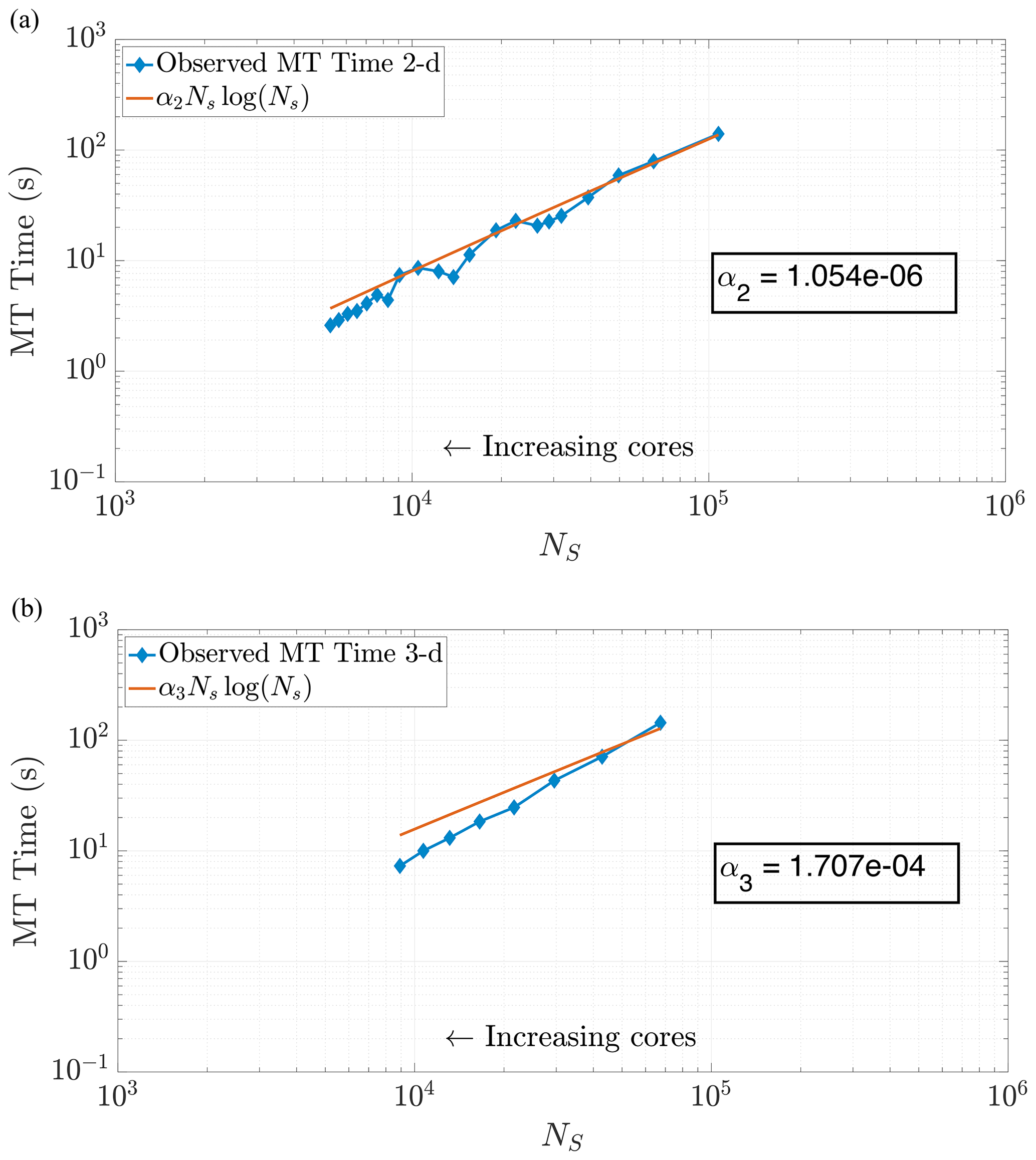
Figure 6Plots of run time in the MT portion of benchmark runs. Note the similar behavior in both 2-D (a) and 3-D (b) for predicting MT subroutine run time, based on our theoretical run time scaling in Eq. (24). Using this prediction function achieves values of r2=0.9780 in 2-D and r2=0.9491 in 3-D. Axis bounds are chosen for ease of comparison to results in Figs. 7, 8, and 10a.
Note that changing the total number of particles within a simulation should not change the scaling relationship as Eq. (24) only depends on the value of NS. This relationship implies that a simulation with a greater number of particles and using a greater number of cores can achieve the same value of NS as a simulation with fewer total particles and cores. When the values of NS coincide across these combinations of particles and cores, we expect the time spent in the MT subroutine to be the same (Figs. 7 and 8). We see that our predictions for the MT subroutine, based on proportionality to the k-D tree search, provide a reliable run time estimate in both the 2-D and 3-D cases. We also observe an overlay in the curves as N increases, which directly increases the amount of work for the MT portion of the algorithm. For instance, if we consider a range of particle numbers in both dimensions (Figs. 7 and 8), we see the respective curves exhibit similar run time behavior as NS decreases.
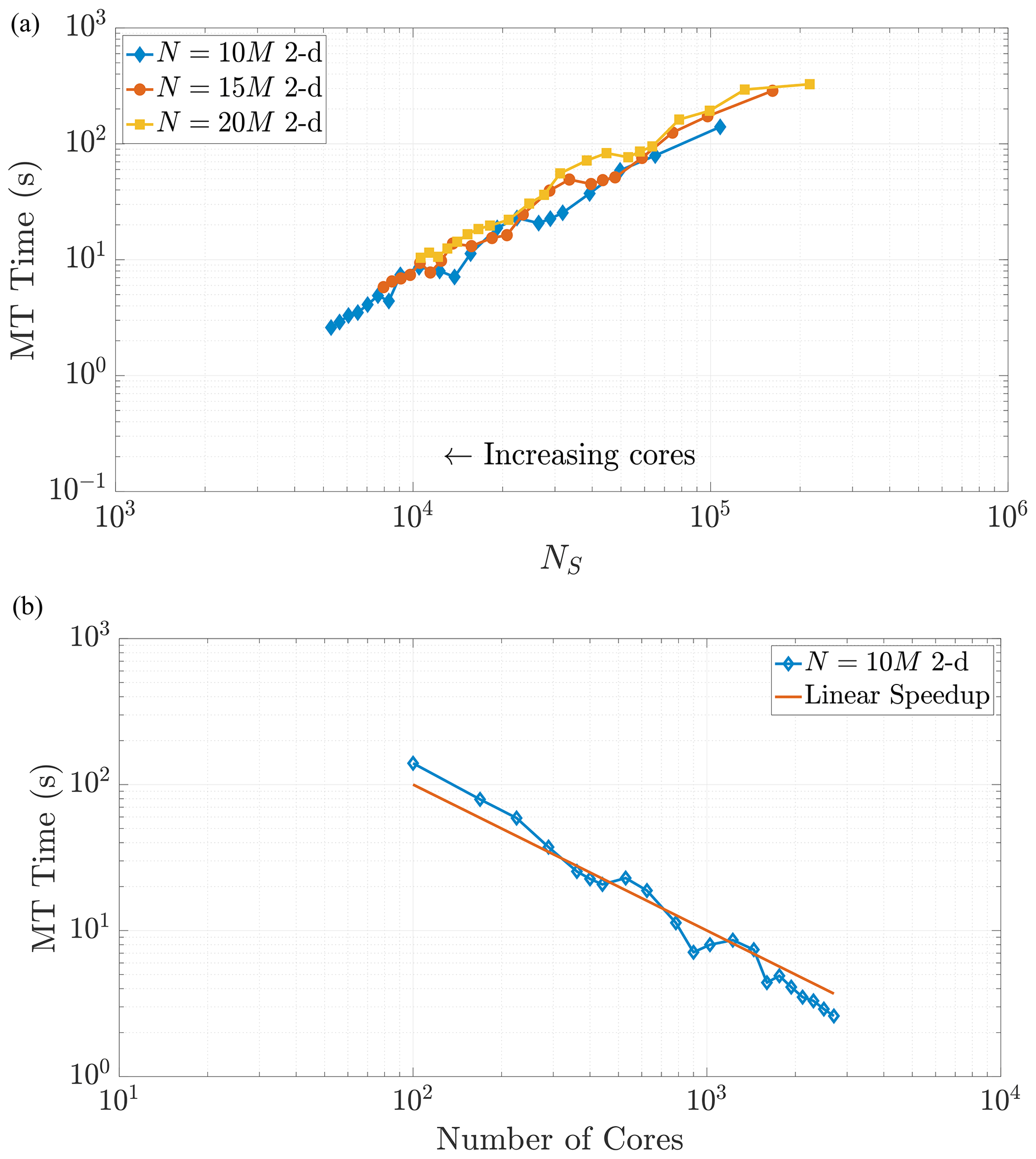
Figure 7Varying the total particle number N directly influences the value of NS, as the rightmost side of Eq. (23) reflects. Simulations across these different values of N in 2-D exhibit common behavior with respect to MT run time as NS decreases, as shown in (a). Panel (b) shows the strong scaling behavior for the 10 M particle simulation for comparison to a common scaling metric. Axis limits are chosen for comparison with Fig. 10a.
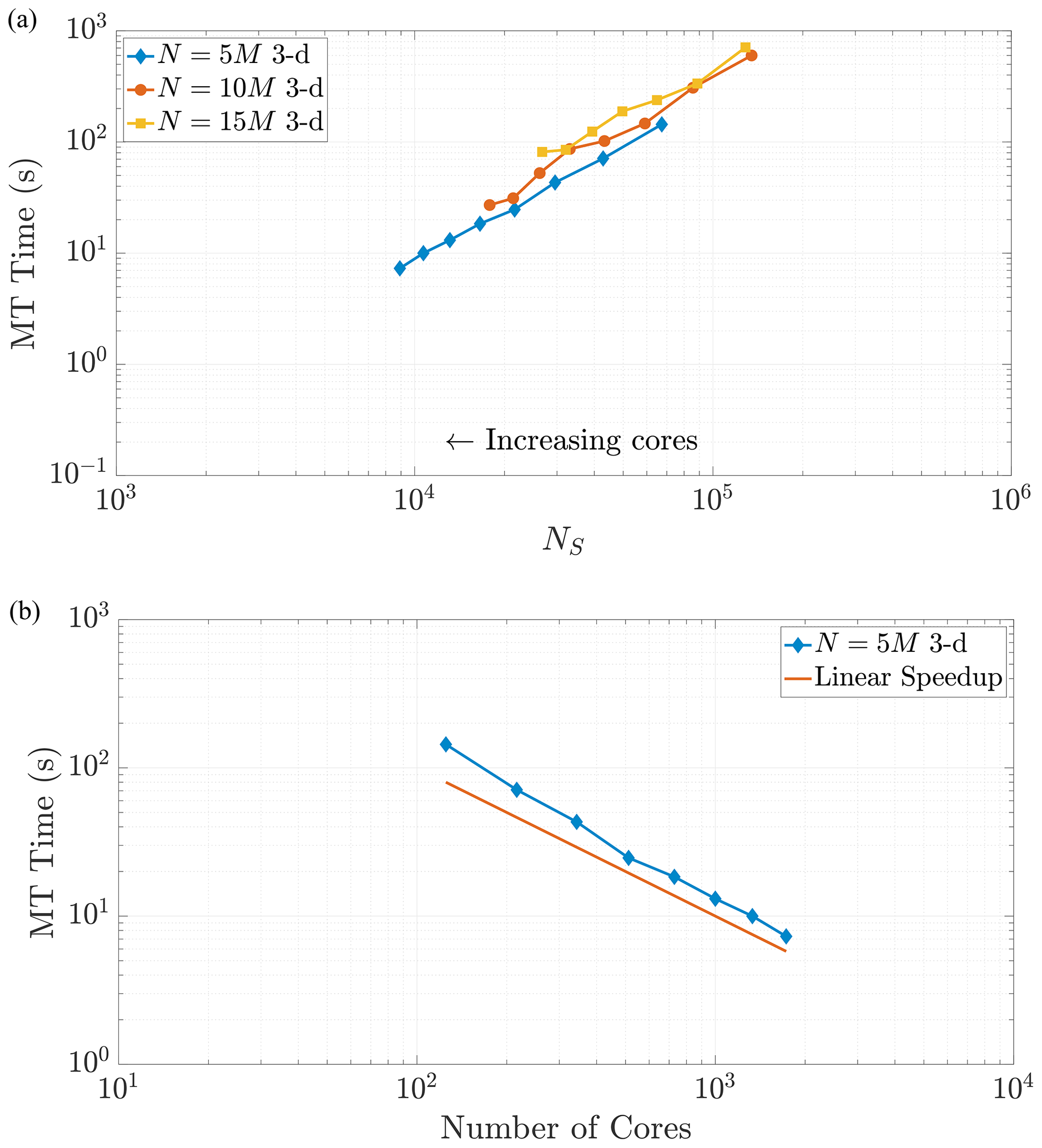
Figure 8Varying the total particle number N directly influences the value of NS, as the rightmost side of Eq. (23) reflects. Simulations across these different values of N in 3-D exhibit common behavior with respect to MT run time as NS decreases, as shown in (a). Panel (b) shows the strong scaling behavior for the 10 M particle simulation for comparison to a common scaling metric. Axis limits are chosen for comparison with Fig. 10a. The scaling is strongly similar to the 2-D example.
The plots of MT run time display an approximately linear decrease as NS decreases, which would seem to indicate continued performance gains with the addition of more cores. However, one must remember that adding cores is an action of diminishing returns because the local core areas or volumes tend to zero as more are added, and NS tends to a constant given by the size of the surrounding ghost particle area (see Fig. 5). For example, Fig. 6a shows that MT run time only decreases by around half of a second from adding nearly 1500 cores. Figures 7 and 8 display (a) weak-like scaling plots and (b) strong scaling plots for the MT portion of the algorithm. Predictions concerning this trade-off are made in Sect. 7.
6.2 Ghost particle communication cost analysis
The halo exchange depicted in Sect. 5 is implemented via a distributed-memory, MPI-based subroutine. Each core in the simulation carries out the communication protocol regardless of on-node or inter-node relationship to its neighboring cores, as shown in Fig. 4b. These explicit, MPI exchange instructions ensure that this communication occurs in a similar fashion between all cores, regardless of node relationship. This claim is substantiated by the single-node scaling seen in Fig. 9, reinforcing that our speedup results are not skewed by redundant or “accelerated” shared-memory communication.
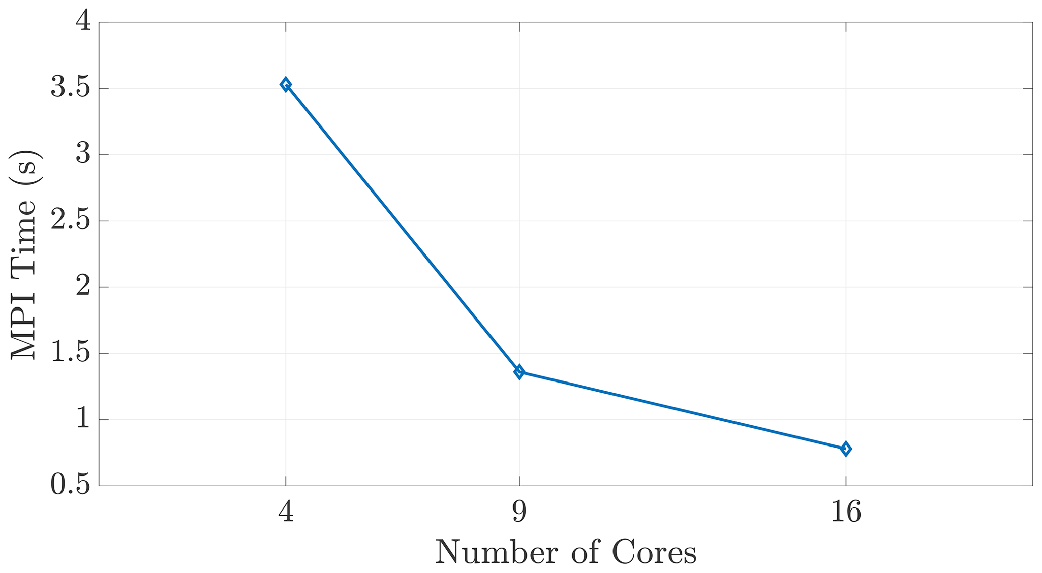
Figure 9We observe expected wall time scaling for the on-node communication shown here, demonstrating that the MPI function calls do, in fact, incur communication costs between cores within a shared-memory space.
The communication portion of the algorithm includes three processes on each core: evaluating logical statements to determine which particles to send to each neighboring core, sending the particles to the neighboring cores, and receiving particles from all neighboring cores. The total wall time for these three processes makes up the “MPI time (s)” in Figs. 9 and 10. By nature of these tiled, halo exchanges, we encounter the issue of load balancing, namely the process of distributing traffic so that cores with less work to do will not need to wait on those cores with more work. Hence, we only need to focus our predictions on the cores that will perform the greatest amount of work. These cores (in both dimensions) are the “interior” subdomains or the subdomains with neighbors on all sides. In 2-D these subdomains will receive particles from eight neighboring domains, with four neighbors sharing edges and four on adjacent corners. In 3-D, particles are shared among 26 neighboring subdomains. Similar to the MT analysis, we observe that both the 2-D and 3-D data in Fig. 10a exhibit similar curves across varying particle numbers as the number of cores becomes large (i.e., as NS becomes small). This eventual constant cost is to be expected in view of the asymptotic behavior of NS as P grows large. Note also that the 3-D MPI simulation times are consistently around 5 to 10 times greater than 2-D because of the increased number of neighboring cores involved in the ghost particle information transfer.
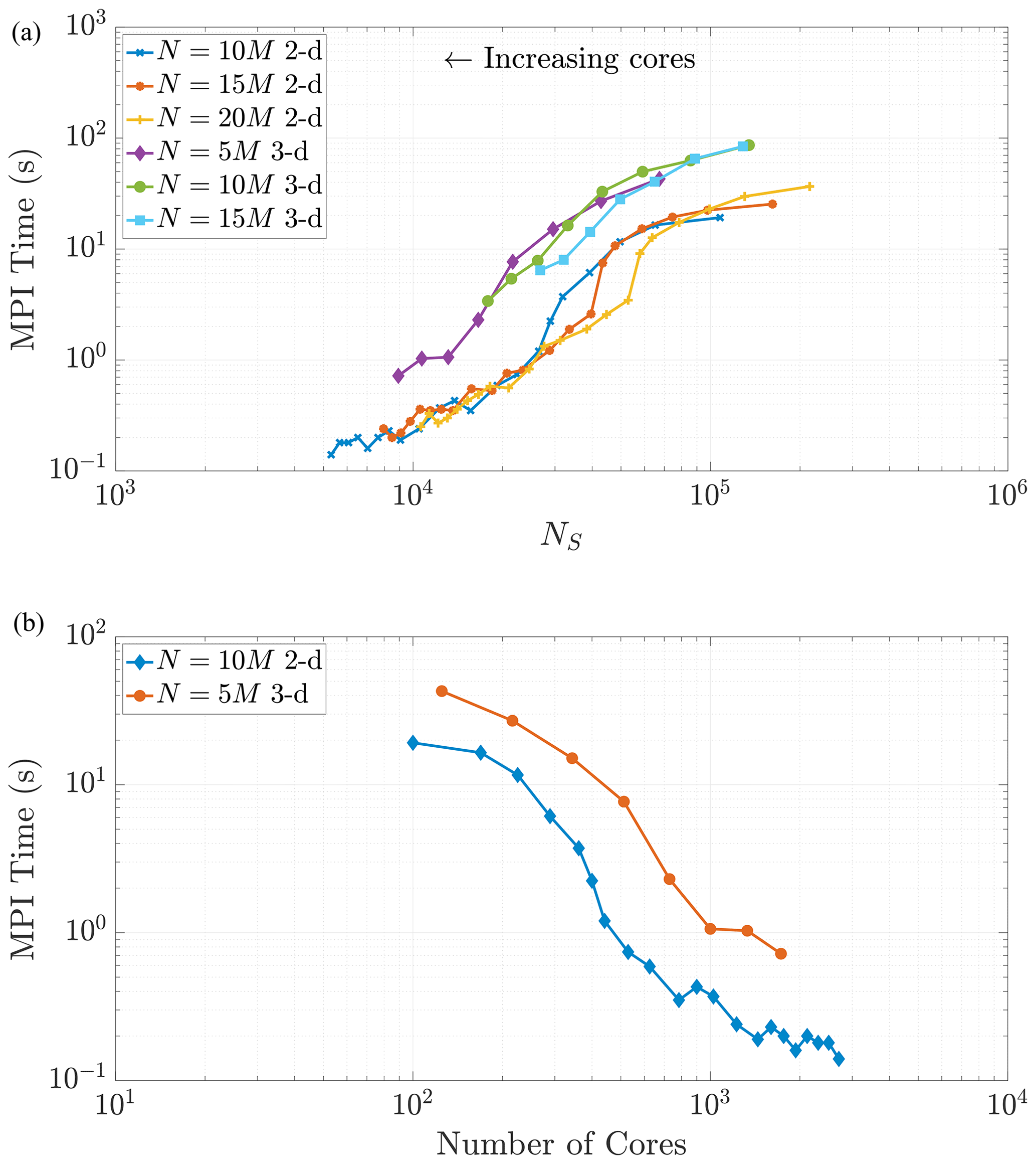
Figure 10As NS decreases, we observe similar trends in the MPI subroutine run time in both 2-D and 3-D. Given that necessary communication takes places between 26 neighboring regions in 3-D rather than only eight neighboring regions in 2-D, the 3-D MPI times are, in general, 5 to 10 times slower than similar runs in 2-D.
In this section, we discuss the advantages and limitations of each method by evaluating the manner in which the decomposition strategies accelerate run times. We employ the quantity “speedup” in order to compare the results of our numerical experiments. The speedup of a parallelized process is commonly formulated as
where TP is the run time using P cores and T1 is the serial run time. We also use the notion of efficiency that relates the speedup to the number of cores and is typically formulated as
If the parallelization is perfectly efficient, then P cores will yield a P times speedup from the serial run, producing a value of EP=1. Hence, we compare speedup performance to establish a method that best suits multi-dimensional simulations.
We may also construct a theoretical prediction of the expected speedup due to the run time analysis of the preceding section. First, assume that the subdomains are ideally configured as squares in 2-D or cubes on 3-D. In this case, the MT run times always exceed the MPI times. For smaller values of NS, the MT run times are approximately 10 to 100 times larger than those of the MPI step. Furthermore, the larger MT times are approximately linear with NS over a large range, regardless of total particle numbers and dimension. Therefore, we may assume that the run times are approximately linear with NS and compare run times for different values of P. Specifically, for a single core, all of the particles contribute to the MT run time, so the speedup can be calculated using Eq. (23) in the denominator:
Now, letting represent a desired efficiency threshold, we can identify the maximum number of cores that will deliver an efficiency of ℰ based on the size L of the domain, the physics of the problem, and the optimal time step Δt that defines the size of the ghost region (given in terms of the pad distance ψ). In particular, using the above efficiency formula, we want
A rearrangement then gives the inequality
which provides an upper bound on the suggested number of cores to use once ψ is fixed and a desired minimum efficiency is chosen.
This gives the user a couple of options before running a simulation. The first option is to choose a desired minimum efficiency and obtain a suggested number of cores to use based on the inequality in Eq. (29). This option is ideal for users who request or pay for the allocation of computational resources and must know the quantity of resources to employ in the simulation. The second option is to choose a value for the number of cores and apply the inequality (28) to obtain an estimated efficiency level for that number of cores. This second case may correspond to users who have free or unrestricted access to large amounts of computing resources and may be less concerned about loss of efficiency.
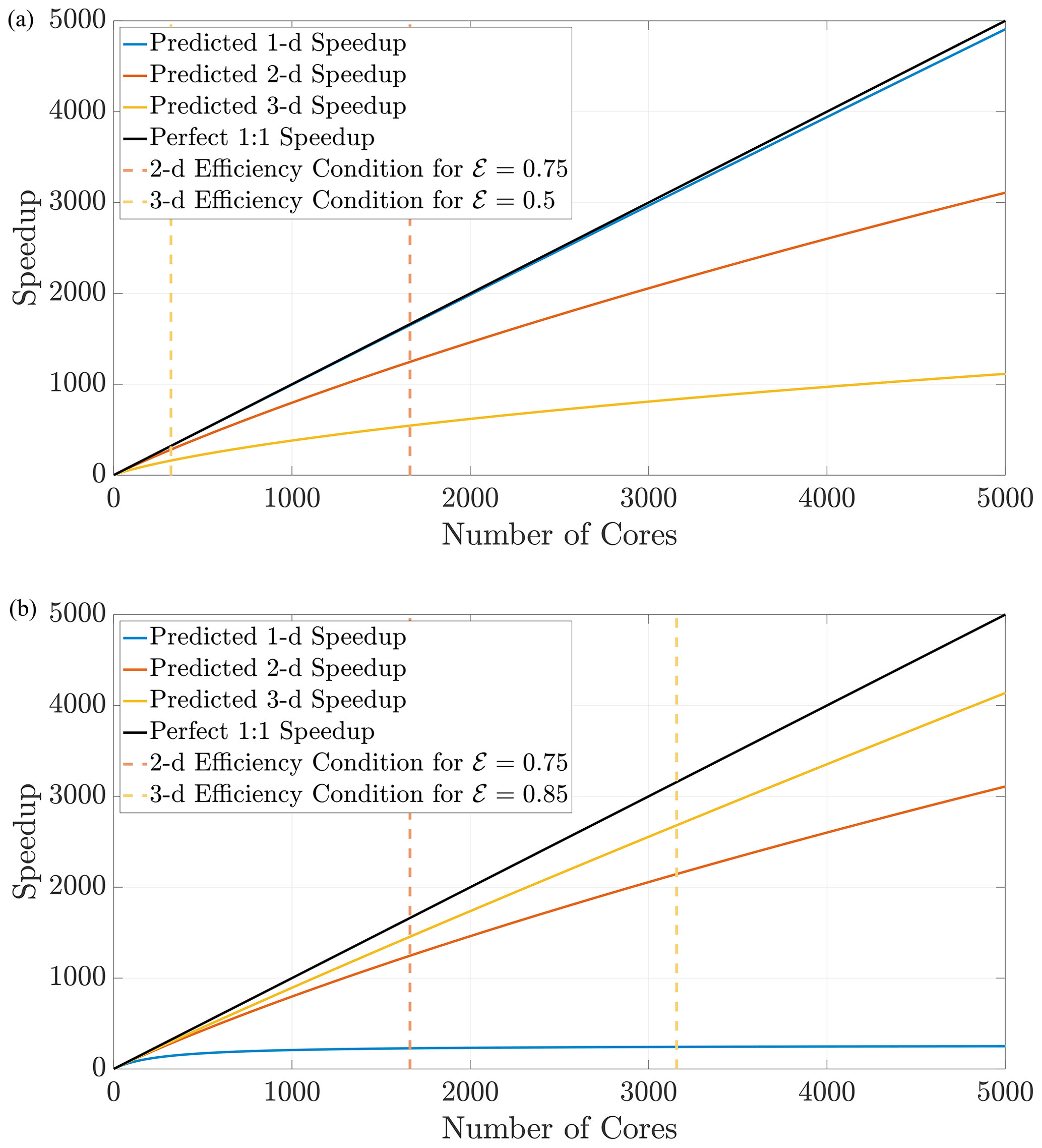
Figure 11The prediction curves give the user a concrete guideline to determine how many cores to allocate for a simulation before performance degrades. The curves in (a) are generated for the defined search distance ψ in a domain with a constant respective hypervolume 𝒱, which implies that each dimension's length scale is . The curves in (b) are generated for the same search distance ψ but with Ld-sized domains for fixed length L.
Using Eq. (27), we can predict speedup performance for any simulation once the parameters are chosen. The speedup prediction inequalities from above depend only on the domain size and the search distance ψ. From these inequalities, the effects of dimensionality while implementing DDC can be conceptualized in two ways. First, if the hypervolume is held constant as dimension changes, particle density also remains constant, which should generally not induce memory issues moving to higher dimensions. This requires choosing a desired hypervolume 𝒱 and then determining a length scale along a single dimension with Figure 11a displays speedup predictions for 1-D, 2-D, and 3-D simulations in domains with equal hypervolumes and fixed D=1 and Δt=0.1. Keeping hypervolume constant shows the cost of complexity with increasing dimensions, which reduces efficiency at larger amounts of cores. Conversely, a physical problem may have a fixed size on the order of L3, and a user may wish to perform upscaled simulations in 1-D and 2-D before running full 3-D simulations. Figure 11b shows the opposite effect: for a fixed length scale L, the lower-dimension simulations suffer degraded efficiency for lower number of cores.
The 2-D and 3-D benchmark simulations used in previous sections allow us to calculate both the empirical (observed) and theoretical speedups, and the overlays in Figs. 12 and 13 show reasonably accurate predictions over a large range of core numbers. The observed run times were averaged over an ensemble of five simulations in order to decrease noise. If the checkerboard method is used to decompose the domain, significantly more cores can be used before the inequality (29) is violated for a chosen efficiency. In particular, if we choose a sequence of perfect square core numbers for the a 1000×1000 domain, nearly linear speedup is observed for over 1000 cores and a maximum of 1906 times speedup at 2700 cores, the largest number of CPU cores to which we had access. For reference, the 1906 times speedup performs a 5 h serial run in 8 s, representing around 0.04 % of the original computational time.
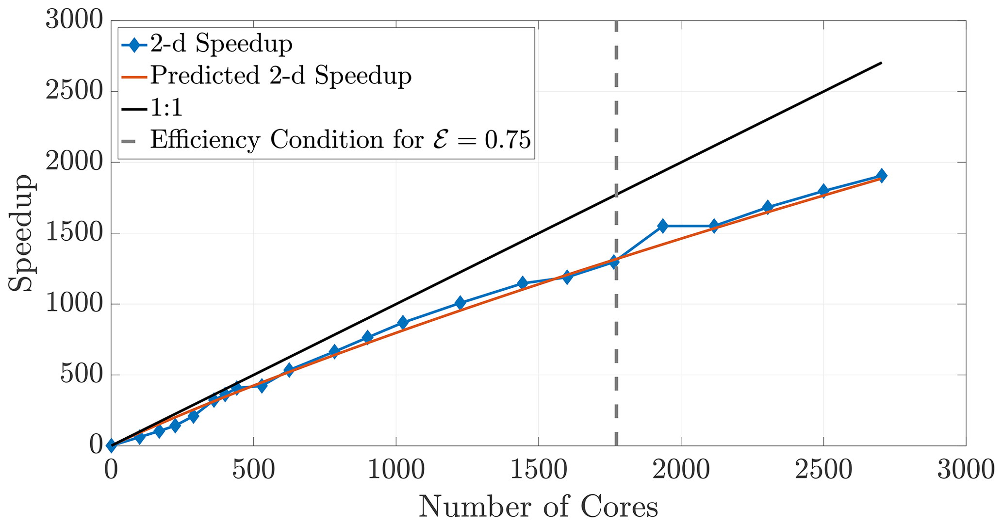
Figure 12Observed (diamonds) and theoretical speedup for 2-D simulations. Each chosen number of cores is a perfect square so that the checkerboard method gives square subdomains. With the chosen parameters L=1000, D=1, and Δt=0.1 and a desired efficiency of 0.75, the upper bound given by the inequality (29) is not violated for the checkerboard method until around 1700 cores.
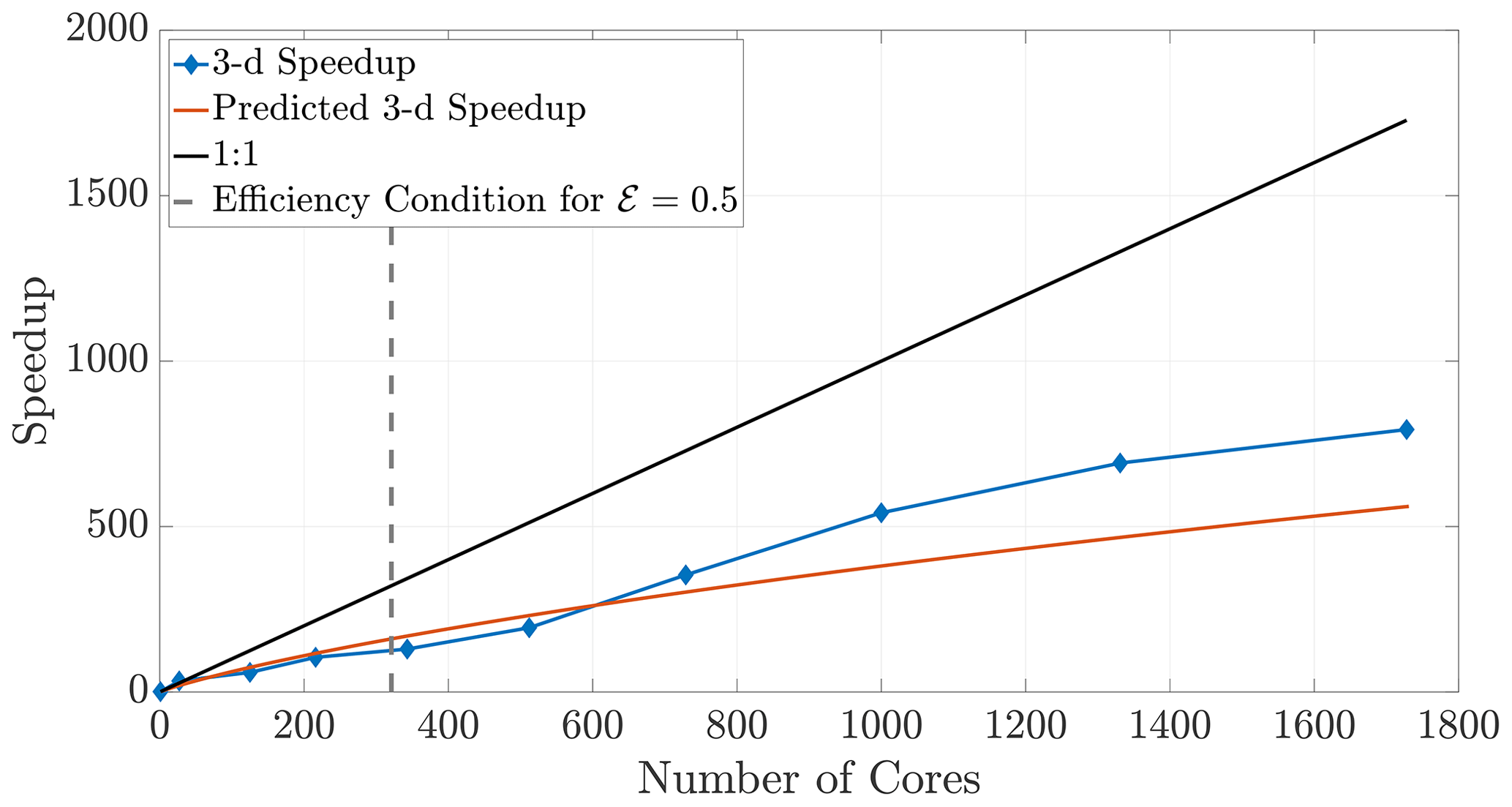
Figure 13Observed (diamonds) and theoretical speedup for 3-D simulations. Each chosen number of cores is a perfect cube so that the checkerboard method gives cubic subdomains. With the chosen parameters L=100, D=1, and Δt=0.1 and a desired efficiency of 0.5, the upper bound given by the inequality (29) is not violated for the checkerboard method until around 320 cores.
Finally, we briefly consider the slices method, as it has drastic limitations in 2-D and 3-D. Increasing the number of cores used in a simulation while ψ remains fixed causes the ghost regions (as pictured in Fig. 4a) to comprise a larger ratio of each local subdomain's area. Indeed, if each subdomain sends the majority of its particles, we begin to observe decreased benefits of the parallelization. An inspection of Fig. 4a suggests that the slices method in 2-D will scale approximately like a 1-D system because the expression for NS (Eq. 23) is proportional to the 1-D expression. Indeed, the slices method speedup is reasonably well predicted by the theoretical model for a 1-D model (Fig. 14). Furthermore, because the slices method only decomposes the domain along a single dimension, it violates the condition given in Eq. (29) at lesser numbers of cores than for the checkerboard method. In fact, using too many cores with the slices method can cease necessary communication altogether once a single buffer becomes larger than the subdomain width. For the given parameter values, this phenomenon occurs at 500 cores with the slices method, so we do not include simulations beyond that number of cores. The speedup for the slices method up to 500 cores is shown in Fig. 14. Although the algorithm is accurate up to 500 cores, we see that performance deteriorates quite rapidly after around 100 cores, which motivated the investigation of the checkerboard decomposition.
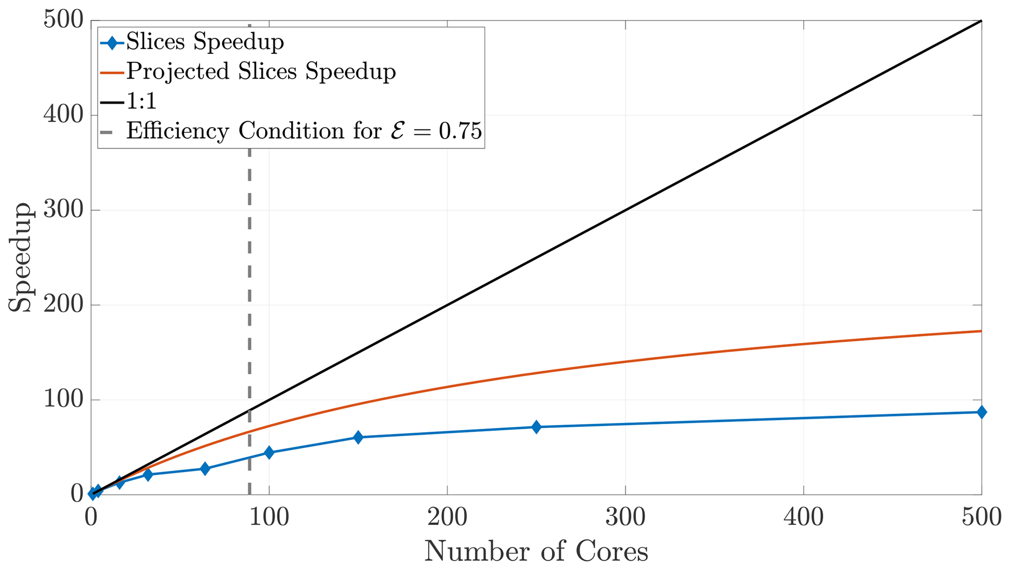
Figure 14Speedup for the slices method plateaus quickly, as the ghost regions increase in proportion to the local subdomain's area.
7.1 Non-square tilings and checkerboard cautions
Given some fixed number of cores (hence subdomains), it is clear that using a subdomain tiling that is as close as possible to a perfect square (or cube) maximizes efficiency. This occurs when the factors for subdivisions in each dimension are chosen to most closely resemble the aspect ratio of the entire domain (shown in 2-D in Eq. 20). Square or cubic subdomains are the most efficient shape to use and result in improved speedup that extends to larger numbers of cores. The converse of this principle means that a poor choice of cores (say, a prime number) will force a poor tiling, and so certain choices for increased core numbers can significantly degrade efficiency. Figure 15 depicts results in 2-D for core numbers of P=698 (with nearest integer factors of 2 and 349) and P=1322 (with nearest integer factors of 2 and 661) along with well-chosen numbers of cores, namely the perfect squares P=400 and P=1600. It is clear from the speedup plot that simulations with poorly chosen numbers of cores do not yield efficient runs relative to other choices that are much closer to the ideal linear speedup. In particular, we note that the speedup in the case of nearly prime numbers of cores is much closer to the anticipated 1-D speedup. This occurs due to the subdomain aspect ratio being heavily skewed and therefore better resembling a 1-D subdomain rather than a regular (i.e., square) 2-D region.
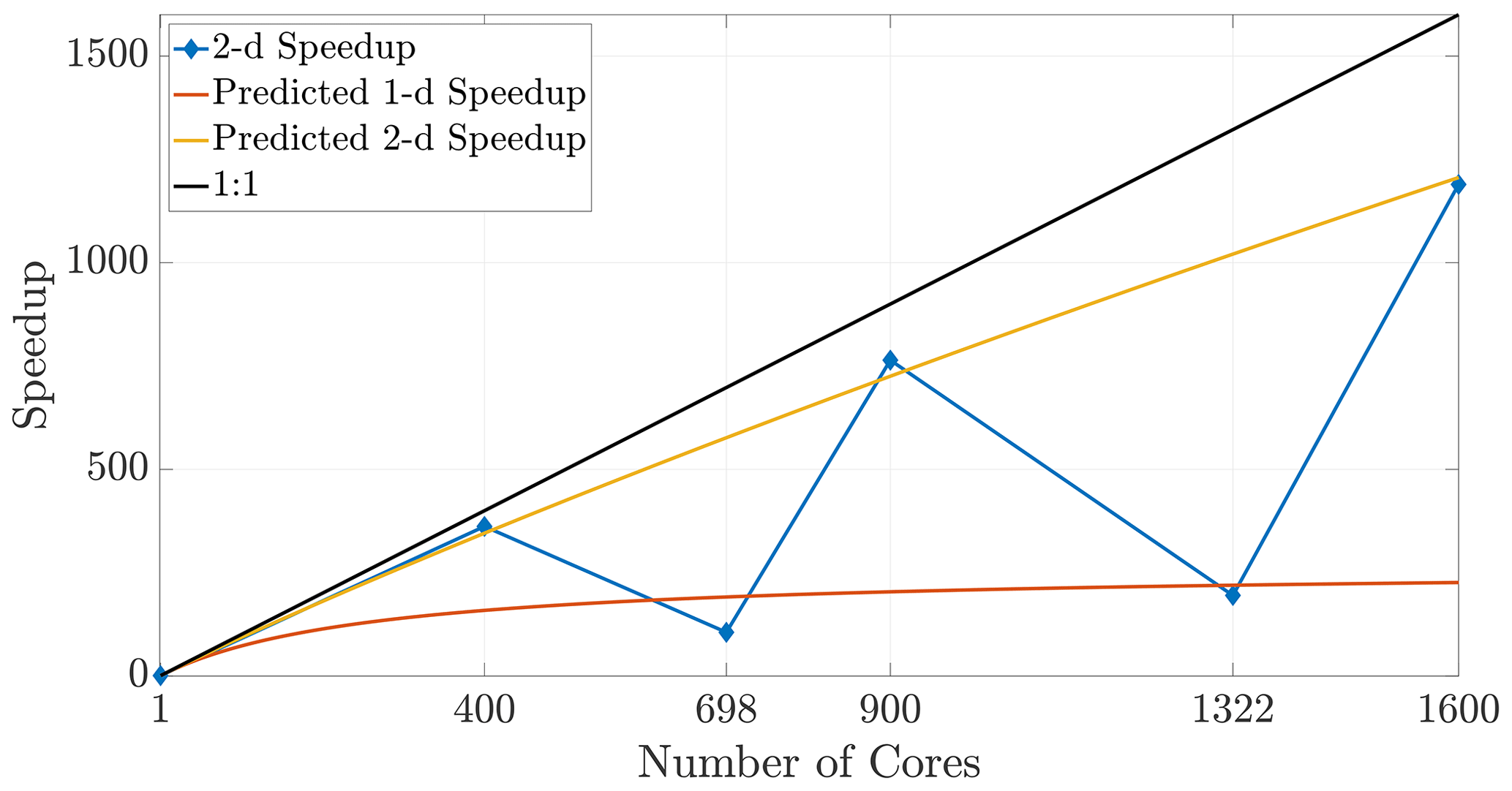
Figure 15Poorly chosen core numbers may result in severely non-square tilings that can degrade speedup performance, despite employing more computational resources.
7.2 Non-serial speedup reference point
We can loosely describe the standard definition of speedup as the quantitative advantage a simulation performed with P cores displays over a simulation running with just a single core. However, a serial run does not require particles to be sent to neighboring regions. Hence, a simulation on a single core does not even enter the MPI subroutine necessary for sending ghost particles, omitting a significant cost. This implies that multi-core simulations have extra cost associated with communication that the serial baseline does not, which is, of course, the reason that linear speedup is difficult to achieve. Unlike the traditional, serial speedup comparison shown in Fig. 12, it is possible to compare speedup results to a 100-core baseline to observe how computational time decreases by adding cores to an already-parallelized simulation. This may be a non-standard metric, but it provides a different vantage point to measure how well an HPC algorithm performs. Further, a metric like this is useful in memory-bound conditions that cannot be conducted on less than 100 cores. Examples of such speedup plots that compare all simulation times to their respective 100-core run times are given in Figs. 16 and 17. More specifically, these figures display the speedup ratio given by
where TP is the run time on P cores and T100 is the run time on 100 cores. For example, with 2500 cores, perfect speedup would be 25 times faster than the 100 core run.

Figure 16A speedup reference point of T100 results in super-linear speedup across multiple particle numbers.
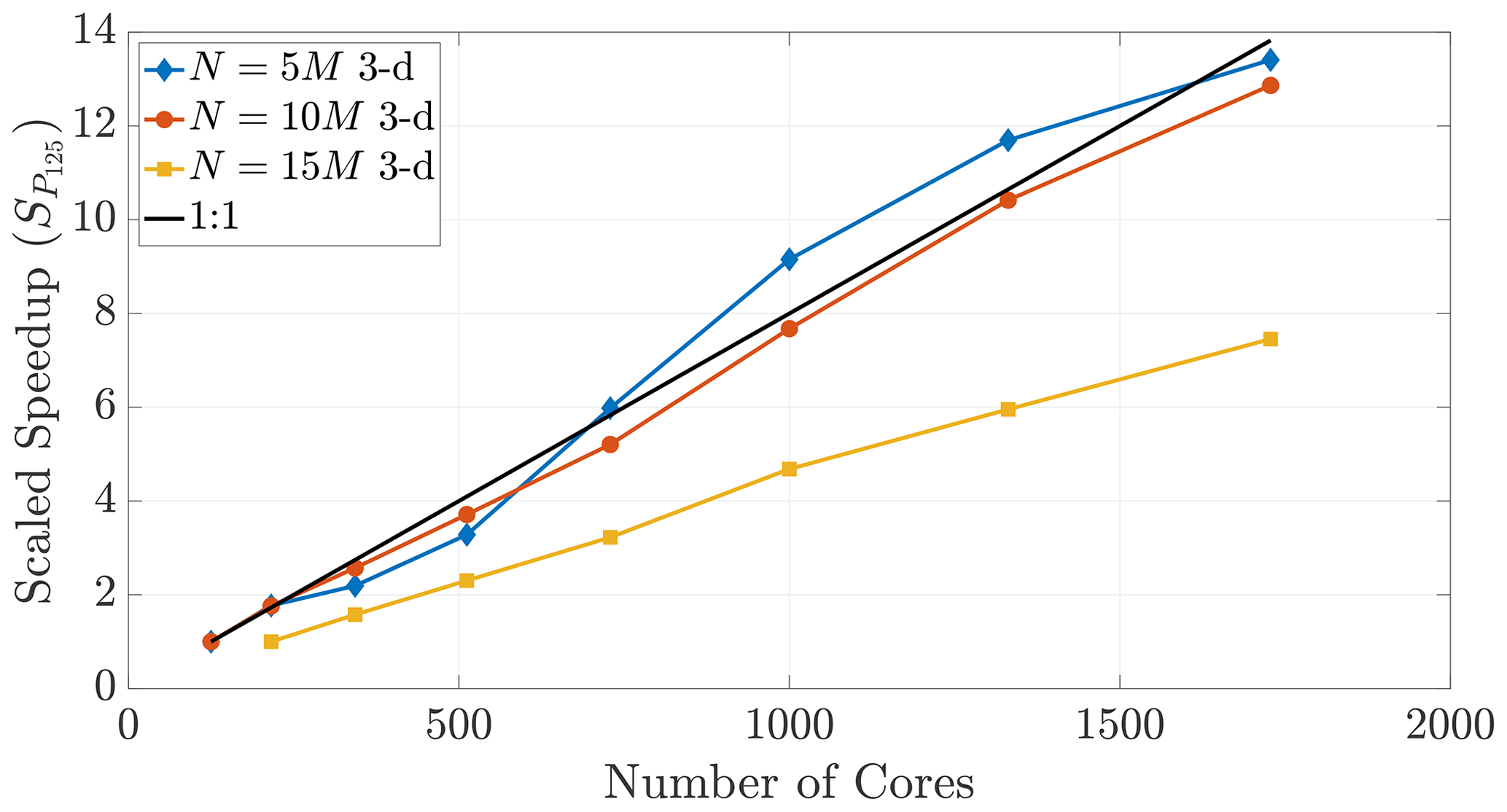
Figure 17Speedup reference points of T125 (and T216 for the 15 M run) result in super-linear speedup for only the N=5 M case, further exemplifying the disparity between 2-D and 3-D.
The performance in Fig. 16 displays super-linear speedup for up to 2700 cores, which shows that memory-restricted simulations using very large particle numbers (i.e., the 15 and 20 M particle data) can be effectively parallelized to much greater numbers of cores. However, Fig. 17 further shows the effect of dimensionality on this comparison, as only those simulations with smaller particle numbers in 3-D achieve super-linear speedup.
The checkerboard decomposition for the parallelized DDC algorithm provides significant speedup to Lagrangian MTPT simulations in multiple dimensions. For a range of simulations, we find that the mass-transfer step is the dominant cost in terms of run time. The approximate linearity of run time with NS (defined as total number of native particles and external ghost particles on a single core/subdomain for mass transfer) allows us to calculate a theoretical speedup that matches empirical results from well-designed DDC domains. The theoretical predictions also allow one to choose an efficiency and calculate the optimal number of cores to use, based on the physics of the problem (specifically, in the context of the benchmarks, we explore domain size L, diffusion coefficient D, and time step Δt). As noted in Sect. 7, these predictions provide users with the necessary forecasting ability that is required before running a large-scale HPC simulation.
Given that we assume a purely diffusive, non-reactive system in this paper, a necessary extension of this will be an investigation of the performance of these DDC techniques upon adding advection, reactions, or both to the system. The benchmarks we establish in this work provide accurate expectations for properly load-balanced problems as we begin to add these complexities into the simulations. In particular, in future efforts we expect to handle variable velocity fields with an adaptable, moving DDC strategy similar to the technique that we implement in this paper. This initial study is an essential prerequisite before other such advances can even begin. Further, using local averaging and interpolation of the corresponding velocity-dependent dispersion tensors, we retain accurate representation of small-scale spreading and mixing despite the subdivided simulation domain. We expect that adequately load balanced, advective-reactive simulations in the future will exhibit as good as or even better scaling than we have observed in these current benchmarks. Moving particles via advection is a naturally parallel computation and will only incur minor computational cost as particles move across subdomain boundaries. Moreover, since the general form of our algorithm simulates complex chemical reactions on particles after mass transfer takes place for all species, we change the most computationally expensive process (the reactions) into a naturally parallel process. Simulating these extra physical phenomena strictly increases computational complexity, but it will be in addition to the computations we carry out here. Given that we are building on these computations, we fully intend to preserve the predictive ability in more complex simulations moving forward. Finally, another natural extension could address various computational questions by exploring how parallelized MTPT techniques might be employed using shared-memory parallelism, such as OpenMP, CUDA, or architecture-portable parallel programming models like Kokkos, RAJA, or YAKL (Edwards et al., 2014; Trott et al., 2022; Beckingsale et al., 2019; RAJA Performance Portability Layer, 2022; Norman, 2022). As we have noted, sending and receiving particles during each time step is a large cost in these simulations, second only to the creation and search of k-D trees and the forward matrix multiplication for mass transfer. Thus, if we could implement a similar DDC technique without physically transmitting ghost particle information between cores and their memory locations, would we expect to see improved speedup for much larger thread counts? A comparison of simulations on a CPU shared memory system to those on a GPU configuration would represent a natural next step to address this question. In this case, we predict that the GPU would also yield impressive speedup, but it is unclear as to which system would provide lesser overall run times given the significant differences in computational and memory architectures between GPU and CPU systems.
In summary, the checkerboard method in 2-D (and 3-D) not only allows simulations to be conducted using large numbers of cores before violating the maximum recommended core condition given in Eq. (29) but also boasts impressive efficiency scaling at a large number of cores. Under the guidelines we prescribe, this method achieves almost perfect linear speedup for more than 1000 cores and maintains significant speedup benefits up to nearly 3000 cores. Our work also showcases how domain decomposition and parallelization can relieve memory-constrained simulations. For example, some of the simulations that we conduct with large numbers of particles cannot be performed with fewer cores due to insufficient memory on each core. However, with a carefully chosen DDC strategy, we can perform simulations with particle numbers that are orders of magnitude greater than can be accomplished in serial, thereby improving resolution and providing higher-fidelity results.
Roofline model analysis provides an understanding of the baseline computational performance of an algorithm by observing the speed and intensity of its implementation on a specific problem and comparing it to the hardware limitations. Thus, this analysis depicts the speed of an algorithm relative to the difficulty of the associated problem. We include this analysis to demonstrate that our single-core baseline result (orange circle in Fig. A1) is as fast and efficient as the hardware bandwidth allows. This ensures that speedup results are not inflated by a suboptimal baseline. These results were produced using LIKWID (Treibig et al., 2010; Roehl et al., 2014), a tool created by the National Energy Research Scientific Computing Center to measure hardware limitations and algorithmic performance. By varying the particle density within our simulations, we show that the parameters we use for our baseline result perform closer to the bandwidth limit at the respective arithmetic intensity when compared to surrounding particle numbers. For the memory limits of the hardware we employ, we have chosen the parameter combination that yields the most efficient baseline simulation prior to parallelization.

Figure A1This figure displays the full roofline plot with an enlarged inset to accentuate the data trends. The data points correspond to various particle densities while domain size is held constant. As arithmetic intensity fluctuates, we observe that the algorithm's performance is limited by the hardware's bandwidth. We use the chosen parameter set (orange circle) for our speedup results since it (1) is the most efficient, (2) displays high accuracy from its particle count, and (3) is not memory-bound and does not require exceedingly long simulation times.
Fortran/MPI codes for generating all results in this paper are held in the public repository at https://doi.org/10.5281/zenodo.6975289 (Schauer, 2022).
LS was responsible for writing the original draft and creating the software. LS, SDP, DAB, and DB were responsible for conceptualization. LS, NBE, and MJS were responsible for methodology. DAB and SDP were responsible for formal analysis. All authors were responsible for reviewing and editing the paper.
The contact author has declared that none of the authors has any competing interests.
This paper describes objective technical results and
analysis. Any subjective views or opinions that might be expressed in the paper do
not necessarily represent the views of the U.S. Department of Energy or the United
States Government.
Publisher's note: Copernicus Publications remains neutral with regard to jurisdictional claims in published maps and institutional affiliations.
Sandia National Laboratories is a multi-mission laboratory managed and operated by the National Technology and Engineering Solutions of Sandia, L.L.C., a wholly owned subsidiary of Honeywell International, Inc., for the DOE's National Nuclear Security Administration under contract DE-NA0003525. This research used resources of the National Energy Research Scientific Computing Center, which is supported by the Office of Science of the U.S. Department of Energy under contract no. DE-AC02-05CH11231.
The authors and this work were supported by the US Army Research Office (grant no. W911NF-18-1-0338) and by the National Science Foundation (grant nos. CBET-2129531, EAR-2049687, EAR-2049688, DMS-1911145, and DMS-2107938).
This paper was edited by David Ham and reviewed by two anonymous referees.
Aris, R.: On the dispersion of a solute in a fluid flowing through a tube, P. Roy. Soc. Lond. A, 235, 67–77, 1956. a
Bear, J.: On the tensor form of dispersion in porous media, J. Geophys. Res., 66, 1185–1197, https://doi.org/10.1029/JZ066i004p01185, 1961. a
Bear, J.: Dynamics of Fluids in Porous Media, Dover Publications, ISSN 2212-778X, 1972. a
Beckingsale, D. A., Burmark, J., Hornung, R., Jones, H., Killian, W., Kunen, A. J., Pearce, O., Robinson, P., Ryujin, B. S., and Scogland, T. R.: RAJA: Portable Performance for Large-Scale Scientific Applications, in: 2019 IEEE/ACM International Workshop on Performance, Portability and Productivity in HPC (P3HPC), 71–81, https://doi.org/10.1109/P3HPC49587.2019.00012, 2019. a
Benson, D. A. and Bolster, D.: Arbitrarily Complex Chemical Reactions on Particles, Water Resour. Res., 52, 9190–9200, https://doi.org/10.1002/2016WR019368, 2016. a, b
Benson, D. A. and Meerschaert, M. M.: Simulation of chemical reaction via particle tracking: Diffusion-limited versus thermodynamic rate-limited regimes, Water Resour. Res., 44, W12201, https://doi.org/10.1029/2008WR007111, 2008. a, b
Benson, D. A., Aquino, T., Bolster, D., Engdahl, N., Henri, C. V., and Fernàndez-Garcia, D.: A comparison of Eulerian and Lagrangian transport and non-linear reaction algorithms, Adv. Water Resour., 99, 15–37, https://doi.org/10.1016/j.advwatres.2016.11.003, 2017. a, b, c
Benson, D. A., Pankavich, S., and Bolster, D.: On the separate treatment of mixing and spreading by the reactive-particle-tracking algorithm: An example of accurate upscaling of reactive Poiseuille flow, Adv. Water Resour., 123, 40–53, https://doi.org/10.1016/j.advwatres.2018.11.001, 2019. a, b, c
Bentley, J. L.: Multidimensional Binary Search Trees Used for Associative Searching, Commun. ACM, 18, 509–517, https://doi.org/10.1145/361002.361007, 1975. a
Bolster, D., Paster, A., and Benson, D. A.: A particle number conserving Lagrangian method for mixing-driven reactive transport, Water Resour. Res., 52, 1518–1527, https://doi.org/10.1002/2015WR018310, 2016. a, b
Crespo, A., Dominguez, J., Barreiro, A., Gómez-Gesteira, M., and Rogers, B.: GPUs, a New Tool of Acceleration in CFD: Efficiency and Reliability on Smoothed Particle Hydrodynamics Methods, PLoS ONE, 6, e20685, https://doi.org/10.1371/journal.pone.0020685, 2011. a
Dentz, M., Le Borgne, T., Englert, A., and Bijeljic, B.: Mixing, spreading and reaction in heterogeneous media: A brief review, J. Contam. Hydrol., 120–121, 1–17, https://doi.org/10.1016/j.jconhyd.2010.05.002, 2011. a, b
Ding, D., Benson, D. A., Fernández-Garcia, D., Henri, C. V., Hyndman, D. W., Phanikumar, M. S., and Bolster, D.: Elimination of the Reaction Rate “Scale Effect”: Application of the Lagrangian Reactive Particle-Tracking Method to Simulate Mixing-Limited, Field-Scale Biodegradation at the Schoolcraft (MI, USA) Site, Water Resour. Res., 53, 10411–10432, https://doi.org/10.1002/2017WR021103, 2017. a, b
Edwards, H. C., Trott, C. R., and Sunderland, D.: Kokkos: Enabling manycore performance portability through polymorphic memory access patterns, J. Parall. Distrib. Comput., 74, 3202–3216, https://doi.org/10.1016/j.jpdc.2014.07.003, 2014. a
Engdahl, N., Schmidt, M., and Benson, D.: Accelerating and Parallelizing Lagrangian Simulations of Mixing‐Limited Reactive Transport, Water Resour. Res., 55, 3556–3566, https://doi.org/10.1029/2018WR024361, 2019. a, b, c
Engdahl, N. B., Benson, D. A., and Bolster, D.: Lagrangian simulation of mixing and reactions in complex geochemical systems, Water Resour. Res., 53, 3513–3522, https://doi.org/10.1002/2017WR020362, 2017. a
Gelhar, L. W., Gutjahr, A. L., and Naff, R. L.: Stochastic analysis of macrodispersion in a stratified aquifer, Water Resour. Res., 15, 1387–1397, https://doi.org/10.1029/WR015i006p01387, 1979. a, b
Gomez-Gesteira, M., Crespo, A., Rogers, B., Dalrymple, R., Dominguez, J., and Barreiro, A.: SPHysics – development of a free-surface fluid solver – Part 2: Efficiency and test cases, Comput. Geosci., 48, 300–307, https://doi.org/10.1016/j.cageo.2012.02.028, 2012. a
Graham, S. L., Kessler, P. B., and McKusick, M. K.: Gprof: A Call Graph Execution Profiler, SIGPLAN Not., 39, 49–57, https://doi.org/10.1145/989393.989401, 2004. a
Herrera, P. A., Massabó, M., and Beckie, R. D.: A meshless method to simulate solute transport in heterogeneous porous media, Adv. Water Resour., 32, 413–429, https://doi.org/10.1016/j.advwatres.2008.12.005, 2009. a
Kennel, M. B.: KDTREE 2: Fortran 95 and C++ Software to Efficiently Search for Near Neighbors in a Multi-Dimensional Euclidean Space, arXiv Physics, https://arxiv.org/abs/physics/0408067v2 (last access: 11 August 2022), 2004. a
LaBolle, E. M., Fogg, G. E., and Tompson, A. F. B.: Random-Walk Simulation of Transport in Heterogeneous Porous Media: Local Mass-Conservation Problem and Implementation Methods, Water Resour. Res., 32, 583–593, https://doi.org/10.1029/95WR03528, 1996. a, b
Li, L., Maher, K., Navarre-Sitchler, A., Druhan, J., Meile, C., Lawrence, C., Moore, J., Perdrial, J., Sullivan, P., Thompson, A., Jin, L., Bolton, E. W., Brantley, S. L., Dietrich, W. E., Mayer, K. U., Steefel, C. I., Valocchi, A., Zachara, J., Kocar, B., Mcintosh, J., Tutolo, B. M., Kumar, M., Sonnenthal, E., Bao, C., and Beisman, J.: Expanding the role of reactive transport models in critical zone processes, Earth-Sci. Rev., 165, 280–301, 2017. a
Molz, F. and Widdowson, M.: Internal Inconsistencies in Dispersion–Dominated Models That Incorporate Chemical and Microbial Kinetics, Water Resour. Res., 24, 615–619, 1988. a
Morvillo, M., Rizzo, C. B., and de Barros, F. P.: A scalable parallel algorithm for reactive particle tracking, J. Comput. Phys., 446, 110664, https://doi.org/10.1016/j.jcp.2021.110664, 2021. a
NERSC: Roofline performance model, https://docs.nersc.gov/tools/performance/roofline/ (last access: 1 January 2023), 2018. a
Norman, M.: YAKL: Yet Another Kernel Library, https://github.com/mrnorman/YAKL (last access: 11 August 2022), 2022. a
Ofenbeck, G., Steinmann, R., Caparros, V., Spampinato, D. G., and Püschel, M.: Applying the roofline model, in: 2014 IEEE International Symposium on Performance Analysis of Systems and Software (ISPASS), 76–85, https://doi.org/10.1109/ISPASS.2014.6844463, 2014. a
Paster, A., Bolster, D., and Benson, D. A.: Particle tracking and the diffusion-reaction equation, Water Resour. Res., 49, 1–6, https://doi.org/10.1029/2012WR012444, 2013. a
Paster, A., Bolster, D., and Benson, D. A.: Connecting the dots: Semi-analytical and random walk numerical solutions of the diffusion–reaction equation with stochastic initial conditions, J. Comput. Phys., 263, 91–112, https://doi.org/10.1016/j.jcp.2014.01.020, 2014. a
Perzan, Z., Babey, T., Caers, J., Bargar, J. R., and Maher, K.: Local and Global Sensitivity Analysis of a Reactive Transport Model Simulating Floodplain Redox Cycling, Water Resour. Res., 57, e2021WR029723, https://doi.org/10.1029/2021WR029723, 2021. a
RAJA Performance Portability Layer: https://github.com/LLNL/RAJA, last access: 11 August 2022. a
Roehl, T., Treibig, J., Hager, G., and Wellein, G.: Overhead Analysis of Performance Counter Measurements, in: 43rd International Conference on Parallel Processing Workshops (ICCPW), 176–185, https://doi.org/10.1109/ICPPW.2014.34, 2014. a
Salamon, P., Fernàndez-Garcia, D., and Gómez-Hernández, J. J.: A review and numerical assessment of the random walk particle tracking method, J. Contam. Hydrol., 87, 277–305, https://doi.org/10.1016/j.jconhyd.2006.05.005, 2006. a, b
Schauer, L.: lschauer95/Parallelized-Mass-Transfer-Domain- Decomposition: Parallelized Domain Decomposition for Mass Transfer Particle Tracking Simulations, Zenodo [code], https://doi.org/10.5281/zenodo.6975289, 2022. a
Scheibe, T. D., Schuchardt, K., Agarwal, K., Chase, J., Yang, X., Palmer, B. J., Tartakovsky, A. M., Elsethagen, T., and Redden, G.: Hybrid multiscale simulation of a mixing-controlled reaction, Adv. Water Resour., 83, 228–239, https://doi.org/10.1016/j.advwatres.2015.06.006, 2015. a
Schmidt, M. J., Pankavich, S., and Benson, D. A.: A Kernel-based Lagrangian method for imperfectly-mixed chemical reactions, J. Comput. Phys., 336, 288–307, https://doi.org/10.1016/j.jcp.2017.02.012, 2017. a
Schmidt, M. J., Pankavich, S. D., and Benson, D. A.: On the accuracy of simulating mixing by random-walk particle-based mass-transfer algorithms, Adv. Water Resour., 117, 115–119, https://doi.org/10.1016/j.advwatres.2018.05.003, 2018. a
Schmidt, M. J., Pankavich, S. D., Navarre-Sitchler, A., and Benson, D. A.: A Lagrangian Method for Reactive Transport with Solid/Aqueous Chemical Phase Interaction, J. Comput. Phys., 2, 100021, https://doi.org/10.1016/j.jcpx.2019.100021, 2019. a, b
Schmidt, M. J., Engdahl, N. B., Pankavich, S. D., and Bolster, D.: A mass-transfer particle-tracking method for simulating transport with discontinuous diffusion coefficients, Adv. Water Resour., 140, 103577, https://doi.org/10.1016/j.advwatres.2020.103577, 2020a. a
Schmidt, M. J., Pankavich, S. D., Navarre-Sitchler, A., Engdahl, N. B., Bolster, D., and Benson, D. A.: Reactive particle-tracking solutions to a benchmark problem on heavy metal cycling in lake sediments, J. Contam. Hydrol., 234, 103642, https://doi.org/10.1016/j.jconhyd.2020.103642, 2020b. a, b
Schmidt, M. J., Engdahl, N. B., Benson, D. A., and Bolster, D.: Optimal Time Step Length for Lagrangian Interacting-Particle Simulations of Diffusive Mixing, Transport Porous Med., 146, 413–433, https://doi.org/10.1007/s11242-021-01734-8, 2022. a
Sole-Mari, G., Fernàndez-Garcia, D., Rodríguez-Escales, P., and Sanchez-Vila, X.: A KDE-Based Random Walk Method for Modeling Reactive Transport With Complex Kinetics in Porous Media, Water Resour. Res., 53, 9019–9039, https://doi.org/10.1002/2017WR021064, 2017. a
Sole-Mari, G., Schmidt, M. J., Pankavich, S. D., and Benson, D. A.: Numerical Equivalence Between SPH and Probabilistic Mass Transfer Methods for Lagrangian Simulation of Dispersion, Adv. Water Resour., 126, 108–115, https://doi.org/10.1016/j.advwatres.2019.02.009, 2019. a, b, c
Sole-Mari, G., Fernandez-Garcia, D., Sanchez-Vila, X., and Bolster, D.: Lagrangian modeling of mixing-limited reactive transport in porous media; multirate interaction by exchange with the mean, Water Resour. Res., 56, e2019WR026993, https://doi.org/10.1029/2019WR026993, 2020. a
Steefel, C. I., Appelo, C. A., Arora, B., Jacques, D., Kalbacher, T., Kolditz, O., Lagneau, V., Lichtner, P. C., Mayer, K. U., Meeussen, J. C., Molins, S., Moulton, D., Shao, H., Šimůnek, J., Spycher, N., Yabusaki, S. B., and Yeh, G. T.: Reactive transport codes for subsurface environmental simulation, Comput. Geosci., 19, 445–478, https://doi.org/10.1007/s10596-014-9443-x, 2015. a
Sun, T., Mitchell, L., Kulkarni, K., Klöckner, A., Ham, D. A., and Kelly, P. H.: A study of vectorization for matrix-free finite element methods, The Int. J. High Perform. Comput. Appl., 34, 629–644, https://doi.org/10.1177/1094342020945005, 2020. a
Taylor, G. I.: Dispersion of soluble matter in solvent flowing slowly through a tube, P. Roy. Soc. Lond. A, 219, 186–203, 1953. a
Tennekes, H. and Lumley, J. L.: A First Course in Turbulence, MIT Press, 1972. a, b
Tompson, A. and Dougherty, D.: On the Use of Particle Tracking Methods for Solute Transport in Porous Media, in: Vol. 2 Numerical Methods for Transport and Hydrologic Processes, edited by: Celia, M., Ferrand, L., Brebbia, C., Gray, W., and Pinder, G., vol. 36 of Developments in Water Science, Elsevier, 227–232, https://doi.org/10.1016/S0167-5648(08)70094-7, 1988. a
Tompson, A. F. B., Falgout, R. D., Smith, S. G., Bosl, W. J., and Ashby, S. F.: Analysis of subsurface contaminant migration and remediation using high performance computing, Adv. Water Resour., 22, 203–221, https://doi.org/10.1016/S0309-1708(98)00013-X, 1998. a
Treibig, J., Hager, G., and Wellein, G.: LIKWID: A lightweight performance-oriented tool suite for x86 multicore environments, in: Proceedings of PSTI2010, the First International Workshop on Parallel Software Tools and Tool Infrastructures, San Diego CA, 2010. a
Trott, C. R., Lebrun-Grandié, D., Arndt, D., Ciesko, J., Dang, V., Ellingwood, N., Gayatri, R., Harvey, E., Hollman, D. S., Ibanez, D., Liber, N., Madsen, J., Miles, J., Poliakoff, D., Powell, A., Rajamanickam, S., Simberg, M., Sunderland, D., Turcksin, B., and Wilke, J.: Kokkos 3: Programming Model Extensions for the Exascale Era, IEEE T. Parall. Distr., 33, 805–817, https://doi.org/10.1109/TPDS.2021.3097283, 2022. a
Valocchi, A. J., Bolster, D., and Werth, C. J.: Mixing-limited reactions in porous media, Transport Porous Med., 130, 157–182, 2019. a
Williams, S., Waterman, A., and Patterson, D.: Roofline: An Insightful Visual Performance Model for Multicore Architectures, Commun. ACM, 52, 65–76, https://doi.org/10.1145/1498765.1498785, 2009. a
Xia, X. and Liang, Q.: A GPU-accelerated smoothed particle hydrodynamics (SPH) model for the shallow water equations, Environ. Model. Softw., 75, 28–43, https://doi.org/10.1016/j.envsoft.2015.10.002, 2016. a
- Abstract
- Introduction
- Model description
- Mass-transfer particle tracking algorithm
- Domain decomposition
- Ghost particles
- Cost analysis
- Speedup results
- Conclusions and final remarks
- Appendix A: Roofline model
- Code and data availability
- Author contributions
- Competing interests
- Disclaimer
- Acknowledgements
- Financial support
- Review statement
- References