Introducing CRYOWRF v1.0: multiscale atmospheric flow simulations with advanced snow cover modelling

Accurately simulating snow cover dynamics and the snow–atmosphere coupling is of major importance for topics as wide-ranging as water resources, natural hazards, and climate change impacts with consequences for sea level rise. We present a new modelling framework for atmospheric flow simulations for cryospheric regions called CRYOWRF. CRYOWRF couples the state-of-the-art and widely used atmospheric model WRF (the Weather Research and Forecasting model) with the detailed snow cover model SNOWPACK. CRYOWRF makes it feasible to simulate the dynamics of a large number of snow layers governed by grain-scale prognostic variables with online coupling to the atmosphere for multiscale simulations from the synoptic to the turbulent scales. Additionally, a new blowing snow scheme is introduced in CRYOWRF and is discussed in detail. CRYOWRF's technical design goals and model capabilities are described, and the performance costs are shown to compare favourably with existing land surface schemes. Three case studies showcasing envisaged use cases for CRYOWRF for polar ice sheets and alpine snowpacks are provided to equip potential users with templates for their research. Finally, the future roadmap for CRYOWRF's development and usage is discussed.

1 Introduction

The cryosphere consists of regions of the Earth where snow and ice cover the surface for some reasonable period during the course of the year. It consists of regions with seasonal snow cover, frozen lakes and rivers, glaciers, continental ice sheets, sea ice, and permafrost and covers a mean total area of 70×10⁶ km² (14 % of Earth's surface area) with sub-annual fluctuations between 82×10⁶ and 57×10⁶ km², depending on the Northern Hemisphere winter season (Ohmura, 2004). Incidentally, the seasonal snow cover, mostly in the Northern Hemisphere, represents the largest surface area (and shortest timescale) of any component of the cryosphere. On the other hand, perennial components of the snow cover, namely glaciers and polar ice sheets in Greenland and Antarctica, cover approximately 16×10⁶ km² of the surface area. Most important is the fact that 80 % of the freshwater on Earth is held in these components, with Antarctica being the largest store, with 90 % of the freshwater ice mass (Ohmura, 2004; Hock et al., 2009).

From the perspective of a land–atmosphere interaction, there is a stark contrast between snow-free and snow-covered regions in terms of mass and energy fluxes. These differences emerge due to the defining material properties of snow, i.e. high albedo, low thermal conductivity, large latent heat for phase change, and low mechanical roughness (Arduini et al., 2019). Betts et al. (2014), for example, showed that simply changing between snow-covered and snow-free conditions results in a 10 K difference in 2 m temperature climatology with all other forcings kept constant. There is, thus, a vast area of the planet where accurately modelling the dynamics of snow cover and its special interaction with the atmosphere is of primary importance.

The cryosphere is studied at different scales with different motivations. At the largest (planetary) scale, accounting for the cryosphere is critical, since it modulates the energy and water budget of the Earth system (Vaughan et al., 2003; Frei et al., 2012). At a regional (or catchment scale), snow cover dynamics play a significant role for water resources for agriculture (Barnett et al., 2005) and hydroelectricity (Schaefli, 2015; Dujardin et al., 2021) on account of its delayed release of water (melting phase) following a prolonged winter season consisting of the accumulation and storage phases. The melting phase of the snow cover is particularly strongly correlated with hazards such as spring floods (Bloeschl et al., 2017) and landslides (Harpold and Kohler, 2017). In some countries with a well-developed ski industry, snow modelling is used extensively to guide the planning and management of skiing assets and, more importantly, for predicting avalanches (Hanzer et al., 2020).

Various numerical models with varying degrees of complexity have been developed to simulate the dynamics of snow cover. Snow models are a primary component of climate models, which until recently had a relatively simplistic description of snow. For example, most participating models in CMIP5 (Taylor et al., 2012) used a single-layer approach, where snow is considered to be an additional layer covering the soil. In these models, snow properties such as albedo evolve via empirical parameterizations. Models following this approach are termed low-complexity models and continue to be used in many numerical weather prediction (NWP) models (for example, the COSMO model's TERRA land surface model by Doms et al., 2011, which is used operationally in many countries in Europe). As explained by Jin et al. (1999) and Arduini et al. (2019), such models are able to represent only a single timescale of snow cover dynamics and are prone to errors at all timescales, ranging from the sub-diurnal to the seasonal. This is due to their neglecting the strong vertical gradients of density and temperature typically found in snowpacks and spatially heterogeneous phase changes. Single-layer models have been shown to inaccurately simulate snow depth and mass balance and allied issues like soil freezing, onset of melt, etc. (Saha et al., 2017; Dutra et al., 2012). While the use of data assimilation can ameliorate these issues for short-term NWP applications, sub-seasonal-, seasonal-, and climate-scale forecasts are severely affected by such issues.

At the other end of the complexity spectrum, sophisticated snow models used for avalanche prediction were developed (Krinner et al., 2018). These models have a multi-layer description of snow with a prognostic description of the grain-scale characteristics of snow, such as grain diameter, sphericity and dendricity, and inter-grain bond sizes and coordination numbers. Various bulk material properties, such as hydraulic and thermal conductivity, albedo, compaction, and settling rates (through viscosity parameterizations), are determined directly from grain-scale properties. Such a level of detail is required for avalanche prediction since a single, thin layer of low-density snow with particular grain characteristics can mechanically destabilize the entire snowpack. Such snow models can be denoted as high-complexity models. Examples of such models are the CROCUS model from France (Vionnet et al., 2012) and SNOWPACK (more on this model in the following paragraphs).

There are models termed intermediate-complexity models that still have the multi-layer representation of snow but rely on parameterizations to derive the bulk properties of snow layers without requiring grain-scale information. These models therefore provide the possibility of representing vertical stratification within snowpacks, while avoiding the relatively expensive computational costs of high-complexity models. These models have been shown to significantly improve the representation of the snow cover and its impact on soil and the atmosphere in various studies (Xue et al., 2003; Burke et al., 2013; Decharme et al., 2016). It is not surprising therefore that, just between CMIP5 and its successor CMIP6 (Eyring et al., 2016), most participating models have adopted multi-layer, intermediate-complexity models (see also the related Earth System Model–Snow Intercomparison Project, ESM-SnowMIP; Krinner et al., 2018; Menard et al., 2019). Only recently has the European Centre for Medium-Range Weather Forecasts (ECMWF) Integrated Forecasting System (IFS) transitioned from a single-layer to a multi-layer treatment of snow (Arduini et al., 2019), heralding the adoption of intermediate-complexity snow models within operational NWP.

In spite of the progression in the complexity of snow treatment in NWP and climate models, the continual increase in computational power and resources, along with the scope and need for further improvement, leads us to believe that coupling between NWP or climate models and high-complexity, advanced snow models is both feasible and required, in particular for resolving complex surface processes such as drifting and blowing snow. In this work, we describe the first version of CRYOWRF, a fully coupled atmosphere–snowpack solver suitable for simulations in both alpine and polar regions. CRYOWRF brings together two state-of-the art models, with WRF (the Weather Research and Forecasting model) being the atmospheric core of the model, while SNOWPACK, a high-complexity snow model, acts as the land surface model (LSM).

This development brings together compelling advantages. WRF is a widely used community model with multi-scale capabilities on account of its non-hydrostatic dynamical core along with domain nesting. This allows simulations from the global scale (with grids sizes of 50–100 km) down to turbulence scales (with grid sizes of 10–50 m) using the same software package. WRF is continuously updated with newer, improved physical parameterizations for all the different model components such as radiation, microphysics, boundary layer schemes, etc. From a user perspective, there are many tutorials available online to learn the entire workflow from compilation, pre-processing of input data, and running the model to post-processing model outputs. Thus, any development extending WRF is likely to reach a lot of potential users. There have been previous efforts in a similar spirit to extend WRF. Collier et al. (2013) followed a similar approach to ours, where they modified the WRF source code to include a detailed snow treatment using the Chemical Mass Balance (CMB) model by Mölg et al. (2008). However, to the best of our knowledge, this model is not publicly available and, additionally, does not include a blowing snow scheme. We also acknowledge the pioneering work in polar meteorological modelling using the polar-optimized version of WRF named Polar-WRF (Hines and Bromwich, 2008). Polar-WRF has adapted existing physical models in WRF, undergone extensive evaluations, and added technical capabilities (such as ingesting frequent sea surface temperature and sea ice masks), many of which are now part of the standard WRF. The most important contribution of Polar-WRF and associated studies is compiling best practices for polar modelling using mesoscale models that have inspired various other models (including our development).

SNOWPACK is a well-established, high-complexity snow model developed at the WSL (Wald, Schnee und Landschaft) Institute for Snow and Avalanche Research (SLF), Davos, Switzerland. It was originally developed for avalanche forecasting and is in fact the operational model for this purpose in Switzerland. Since its original development nearly 2 decades ago, SNOWPACK has been continuously updated to include new physics and has been applied in different topics of cryospheric research, such as snow hydrology (Wever et al., 2015, 2016a, b; Brauchli et al., 2017), sea ice thermodynamics (Wever et al., 2020), snow–forest interaction (Gouttevin et al., 2015), ice-sheets mass balance and thermodynamics (Steger et al., 2017b, a; van Wessem et al., 2021; Keenan et al., 2021), and climate-change-induced impact assessments on snow and snow hydrology (Bavay et al., 2013, 2009; Marty et al., 2017). In all the above applications, SNOWPACK has been forced either with meteorological measurement data or NWP/climate model outputs in an offline setting. CRYOWRF is the first implementation of an online coupling between SNOWPACK and an atmospheric model.

A significant direct physical coupling between the snowpack and the atmosphere is through drifting and blowing snow and its effect on the mass and energy balance of the near-surface atmosphere. Drifting and blowing snow redistributes surface snow spatially, while inducing the enhanced sublimation of (and sometimes deposition on) snow grains and thereby saturating (drying) the near-surface air. Blowing snow is estimated to affect nearly all cryospheric environments (Filhol and Sturm, 2015), and there is evidence of their relevance for topics as disparate as avalanche prediction (Lehning and Fierz, 2008), road safety (Tabler, 2003), hydrology (Groot Zwaaftink et al., 2014), interpretation of ice cores (Birnbaum et al., 2010), remote sensing of snow-covered areas (Warren et al., 1998), and thermomechanical dynamics of sea ice packs (Petrich et al., 2012). In spite of its ubiquitous importance in cryospheric regions, blowing snow models are not included in any of the participating models in CMIP6. There are implementations of blowing snow models in regional-scale climate models (RCMs) such as RACMO (van Wessem et al., 2018; Lenaerts et al., 2012), MAR (Amory et al., 2015, for polar regions), and Meso-NH (Vionnet et al., 2012, for alpine regions). Publicly available versions of WRF do not include any model of this important phenomenon (a recent effort to include a blowing snow model in WRF has been published by Luo et al., 2021. However, the model does not seem to be publicly available). Thus, apart from the coupling between WRF and SNOWPACK, a completely novel blowing snow scheme is implemented and released publicly as a part of CRYOWRF.

In Sect. 2, we describe the three models underlying CRYOWRF, namely WRF, SNOWPACK, and, in particular, the blowing snow scheme, in more detail. We discuss the model capabilities of CRYOWRF and its computational costs in Sect. 3. Three case studies are then described that exemplify the range of applications for CRYOWRF, including a continent-scale simulation over Antarctica for mass balance studies (Sect. 4.1), a multi-scale, three-domain simulation (1 km resolution of the innermost nest) of a hydraulic jump in the vicinity of the Dumont d'Urville station on the east Antarctica coast (Sect. 4.2), and a valley-scale simulation in the Swiss Alps surrounding Davos (Sect. 4.3), for avalanche prediction and hydrology applications. We conclude this article with a summary and outlook for future developments of CRYOWRF (Sect. 5).

2 Models and coupling strategy

2.1 Weather Research and Forecasting Model (WRF)

The Weather Research and Forecasting Model (WRF) is an advanced atmospheric modelling system aimed at both operational numerical weather prediction and research activities. It was originally developed and continues to be managed by the NCAR/MMM (Mesoscale and Microscale Meteorology division, National Centre for Atmospheric Research) from the USA. Due to its completely open-source nature, and the large user community, it has significant contributions from research groups and weather services from around the world.

The Advanced Research WRF (ARW) version of the model (Skamarock et al., 2019) solves the fully compressible, Eulerian non-hydrostatic equations for the three velocity components in Cartesian coordinates in the horizontal along with a terrain-following, hybrid sigma pressure vertical coordinate system with a constant pressure surface as the top boundary. Additional prognostic variables are the moist potential temperature and the geopotential. Optionally, depending on the microphysics and chemistry schemes chosen, dynamics of different hydrometeor and chemical species are also prognostically solved for by using advection–diffusion equations with additional source/sink terms. The primary numerical method is finite differencing for spatial derivatives on an Arakawa C grid, with a flexible grid stretching in the vertical. Time-stepping is done using second or third order Runge–Kutta schemes with faster, internal time-stepping to solve for the acoustic modes. The model is fully parallelized with a hybrid MPI + OpenMP implementation for both the solver and the input–output (I/O) processes. Additional important technical capabilities are the ease of performing multi-scale atmospheric simulations with both one-way and two-way nesting, and start–stop–restart capabilities for all nests. The multiscale capabilities and its community-driven nature made WRF the ideal choice as the atmospheric core of CRYOWRF. CRYOWRF v1.0 is derived from the ARW-WRF v4.2.1, with plans to continuously update to newer versions of WRF as and when they are released.

2.2 SNOWPACK

SNOWPACK, originally developed for avalanche warning (Lehning et al., 1999), has evolved into a multi-purpose model for cryospheric snow–atmosphere interactions with modules for soil/permafrost (Haberkorn et al., 2017), vegetation (Gouttevin et al., 2015), and sea ice (Wever et al., 2020). The core SNOWPACK module solves the heat equation on a dynamic finite element mesh, which evolves with mass changes in ice and snow, such that the identity of layers is preserved. A crucial technical capability of the SNOWPACK model is the possibility for smart merging (splitting) of vertical layers based on their similarity (strong gradients). The most important use of this capability is to allow the user to set a maximum number of layers or a maximum snow depth to simulate. Using transient snow microstructure to determine snow properties such as viscosity, thermal conductivity, or albedo, a very detailed representation of snow processes from settling to phase changes and water transport (Wever et al., 2014) results. Upper boundary conditions for mass and heat include many options, e.g. for initial snow density (Groot Zwaaftink et al., 2013), for snow erosion (Lehning and Fierz, 2008), or for atmospheric stability corrections (Schlogl et al., 2017). The one-dimensional SNOWPACK model has previously been coupled (in an offline sense) with a three-dimensional solver in the atmosphere specifically for snow transport and a spatial description of snow–atmosphere interaction (Lehning et al., 2008). As SNOWPACK accounts for soil and vegetation layers, it can be used as a fully fledged, standalone land surface model (LSM), even for non-glaciated terrain, and indeed has been used as such in the form of its spatially distributed version, Alpine3D (Brauchli et al., 2017). The coupling to WRF is similar in concept, as described further on, with the main difference being transitioning from an offline to an online approach. Grain-scale information of the snowpack is critical for modelling drifting and blowing snow that is strongly governed by the grain size and the cohesion between grains (Comola and Lehning, 2017). This is one of the main motivations for coupling WRF and SNOWPACK. Additionally, online coupling allows for the direct exploration of various feedback processes that the offline approach cannot describe.

2.3 Blowing snow model (BSM)

When wind speeds are larger than a certain threshold value, the shear stress at the snow surface is sufficiently high to dislodge snow grains and entrain them into the air. The larger (and heavier) particles are transported along the surface in ballistic trajectories, rebounding over the snow surface and dislodging additional grains due to collision. This phenomenon, known as saltation, occurs in a very shallow layer, with a thickness of 𝒪(10 cm). The smaller particles are instead picked up by turbulent eddies that transport the particles to much greater heights and over much larger horizontal distances; this is referred to as suspension. Suspension is quite similar in its dynamics to dust or cloud ice. Saltation and suspension together is referred to as blowing snow in this study.

In large-scale atmospheric models, it is impossible to have vertical resolutions close to the surface that can resolve the saltation layer, and thus, it is only the suspension layer that is explicitly solved for, with the saltation layer being completely parameterized and acting as a lower boundary condition for the suspension layer. Thus, in what follows, the blowing snow model actually refers to the model for snow suspension.

The blowing snow model implemented in CRYOWRF is a double-moment scheme that solves prognostic equations for the mass (q_bs; kg kg⁻¹) and number (N_bs; kg⁻¹) mixing ratios of blowing snow particles. These equations are essentially Eulerian advection–diffusion-type equations along with phase changes in sublimation and vapour deposition. They are quite similar to those used to solve for solid-phase hydrometeors such as cloud ice or snow. The blowing snow model is described in much greater detail compared to the previous sections, as it is a novel parameterization complementing WRF and SNOWPACK, which, individually, are established and well-known standalone modelling systems.

The blowing snow scheme in CRYOWRF closely follows the framework by Dery and Yau (2002) and the implementation of blowing snow dynamics in Meso-NH (Lafore et al., 1998; Lac et al., 2018) by Vionnet et al. (2014). The principle difference between our implementation and these previous efforts is in the details of calculating terminal fall velocities and threshold friction velocity for snow transport. These changes are described in the following paragraphs. The intended goal of this section is to describe the implementation of the blowing snow scheme for potential users of CRYOWRF and not to discuss in detail the scientific or physical basis of the choices made and the model's comparison with other previously published models. Those discussions are kept for a future publication. The equations in Einstein notation for q_bs and N_bs, respectively, are as follows:

$$\begin{array}{ll}{\displaystyle \frac{\partial q_{\mathrm{bs}}}{\partial t}}+u_i{\displaystyle \frac{\partial q_{\mathrm{bs}}}{\partial x_i}}& {\displaystyle }=-K_{\mathrm{bs}}{\displaystyle \frac{{\partial }^{\mathrm{2}}{q}_{\mathrm{bs}}}{\partial x_i^{\mathrm{2}}}}{\mathit{\delta }}_{i\mathrm{3}}+{\displaystyle \frac{\partial }{\partial x_i}}\left(q_{\mathrm{bs}}{V}_q{\mathit{\delta }}_{i\mathrm{3}}\right)\\ \text{(1a)}& {\displaystyle }& {\displaystyle }+S_q,{\displaystyle \frac{\partial N_{\mathrm{bs}}}{\partial t}}+u_i{\displaystyle \frac{\partial N_{\mathrm{bs}}}{\partial x_i}}& {\displaystyle }=-K_{\mathrm{bs}}{\displaystyle \frac{{\partial }^{\mathrm{2}}{N}_{\mathrm{bs}}}{\partial x_i^{\mathrm{2}}}}{\mathit{\delta }}_{i\mathrm{3}}+{\displaystyle \frac{\partial }{\partial x_i}}\left(N_{\mathrm{bs}}{V}_N{\mathit{\delta }}_{i\mathrm{3}}\right)\\ \text{(1b)}& {\displaystyle }& {\displaystyle }+S_N,\end{array}$$

where $u_{i=\mathrm{1},\mathrm{2},\mathrm{3}}=(u,v,w)$ are the zonal, meridional, and vertical velocity components of the air, respectively. K_bs is the turbulent diffusion coefficient for blowing snow particles, V_q and V_N are the mass- and number-weighted terminal fall velocities of blowing snow particles, and the S_q and S_N are sink (source) terms to account for sublimation (deposition) of blowing snow particles.

There is a lack of clarity about the values of K_bs. In CRYOWRF, K_bs is taken to be the same as that for turbulent diffusion coefficient for heat following Dery and Yau (1999, 2002). In Vionnet et al. (2014), it is modified to 4 times the equivalent coefficient for heat without any explicit reasoning for the modification. Further research, perhaps using dedicated large-eddy simulations of the sort in Sharma et al. (2018), can be used to derive parameterizations for this parameter.

Linking the mass and number mixing ratios is the two-parameter gamma distribution, similar to that used in various double-moment microphysics schemes (Morrison and Grabowski, 2008; Thompson et al., 2008) and indeed in different blowing snow models (Dery and Yau, 2002; Vionnet et al., 2014). The snow particle size distribution is given by the following:

$$\begin{array}{}\text{(2)}& {\displaystyle }n\left(D\right)=N_{\mathrm{bs}}{\mathit{\rho }}_{\mathrm{air}}{\displaystyle \frac{{\mathit{\lambda }}^{\mathit{\alpha }}{D}^{\mathit{\alpha }-\mathrm{1}}{e}^{-D\mathit{\lambda }}}{\mathrm{\Gamma }\left(\mathit{\alpha }\right)}},\end{array}$$

where D is the particle diameter, Γ is the Gamma function, α and λ are the shape and inverse-scale parameters, respectively, and ρ_air is the air density. The above distribution implies the assumption that blowing snow particles are spherical. The α parameter is usually assumed to be between 2 and 3, and in CRYOWRF, it is chosen to be equal to 3, following Vionnet et al. (2014). Given the assumption of spherical particles and a prescribed α, the parameters λ and the mean particle diameter $\stackrel{\mathrm{‾}}{D}$ can be diagnosed from the mixing ratios as follows:

$$\begin{array}{}\text{(3)}& {\displaystyle }\mathit{\lambda }={\left[{\displaystyle \frac{\mathit{\pi }{\mathit{\rho }}_{\mathrm{i}}}{\mathrm{6}}}{\displaystyle \frac{N_{\mathrm{bs}}}{q_{\mathrm{bs}}}}{\displaystyle \frac{\mathrm{\Gamma }\left(\mathit{\alpha }+\mathrm{3}\right)}{\mathrm{\Gamma }\left(\mathit{\alpha }\right)}}\right]}^{\mathrm{1}/\mathrm{3}},\stackrel{\mathrm{‾}}{D}={\displaystyle \frac{\mathit{\alpha }}{\mathit{\lambda }}},\end{array}$$

where ρ_i is the density of individual blowing snow particles (taken to be that of ice). With α known (or assumed) and λ derived, the full distribution is available at every node of the numerical grid. Note that α is assumed to not vary with height, following Dery and Yau (2001) and Vionnet et al. (2014). This is only partially supported by (limited) measurements (Mann et al., 2000; Nishimura and Nemoto, 2005), but more field data are required to draw conclusions about this assumption.

For the calculation of terminal fall velocities, we deviate from the implementations of Dery and Yau (2002) and Vionnet et al. (2014) and instead follow the best-number-based (X) derivations of Mitchell (1996), Khvorostyanov and Curry (2002), and Sulia and Harrington (2011). Incidentally, this approach is also used in the latest model for cold clouds, ISHMAEL (Jensen et al., 2017). The notable feature of ISHMAEL is that its formulation for fall velocities is applicable for all shapes of the ice habit, with aspect ratios ranging from planar to spherical and columnar ice particles. Considering our assumption of spherical blowing snow particles, the mathematical expressions for our purposes are significantly simplified, as described below.

The best number (X) is defined as follows:

$$\begin{array}{}\text{(4)}& {\displaystyle }X={\displaystyle \frac{\mathrm{4}}{\mathrm{3}}}{\displaystyle \frac{D^{\mathrm{3}}{\mathit{\rho }}_{\mathrm{air}}\left({\mathit{\rho }}_{\mathrm{i}}-{\mathit{\rho }}_{\mathrm{air}}\right)\mathrm{g}}{{\mathit{\eta }}^{\mathrm{2}}}},\end{array}$$

where D is the particle diameter, η is the dynamic viscosity of air, ρ_air and ρ_i are the density of air and blowing snow particles, respectively, and g is the gravitational acceleration. The best number is related to the Reynolds number of the particles, following Mitchell (1996), and is

$$\begin{array}{}\text{(5)}& {\displaystyle }Re=a_m{X}^{b_m}.\end{array}$$

Here, a_m and b_m are fitting coefficients, derived by Mitchell (1996), and functions only of the best number.

The first step in calculating the mass- and number-weighted terminal fall velocities is to derive an expression for terminal fall velocity as a function of particle diameter. To do so, we begin by calculating the mean best number as follows:

$$\begin{array}{}\text{(6a)}& {\displaystyle }\stackrel{\mathrm{‾}}{X}& {\displaystyle }={\displaystyle \frac{\int X\left(D\right)n\left(D\right)\mathrm{d}D}{\int n\left(D\right)\mathrm{d}D}},\text{(6b)}& {\displaystyle }& {\displaystyle }=\mathit{\varphi }{\displaystyle \frac{\mathrm{\Gamma }\left(\mathit{\alpha }+\mathrm{3}\right)}{\mathrm{\Gamma }\left(\mathit{\alpha }\right)}}{\displaystyle \frac{\mathrm{1}}{{\mathit{\lambda }}^{\mathrm{3}}}},\text{where}\mathit{\varphi }={\displaystyle \frac{\mathrm{4}}{\mathrm{3}}}{\displaystyle \frac{{\mathit{\rho }}_{\mathrm{air}}\left({\mathit{\rho }}_{\mathrm{ice}}-{\mathit{\rho }}_{\mathrm{air}}\right)g}{{\mathit{\eta }}^{\mathrm{2}}}}.\end{array}$$

Next, the coefficients a_m and b_m are computed using the mean best number $\left(\stackrel{\mathrm{‾}}{X}\right)$. In what follows, a_m and b_m are always understood to be $a_m\left(\stackrel{\mathrm{‾}}{X}\right)$ and $b_m\left(\stackrel{\mathrm{‾}}{X}\right)$, respectively. Using Eq. (5) and equating it to the standard form of the Reynolds' number, the terminal fall velocity V_t as a function of the particle diameter can be derived as follows:

$$\begin{array}{}\text{(7a)}& {\displaystyle \frac{{\mathit{\rho }}_{\mathrm{air}}{V}_{\mathrm{t}}D}{\mathit{\eta }}}& {\displaystyle }=a_m{X}^{b_m},\text{(7b)}& {\displaystyle }{V}_{\mathrm{t}}& {\displaystyle }={\mathit{\varphi }}^{b_m}{\displaystyle \frac{a_m\mathit{\eta }}{{\mathit{\rho }}_{\mathrm{air}}}}{D}^{\mathrm{3}{b}_m-\mathrm{1}}.\end{array}$$

From a technical perspective, Eq. (7b) is quite useful as it is a continuous and easily integrable function of D of the form $\left(\cdot \right)D^{\left(\cdot \right)}$. From Eq. (7b), equations for V_q and V_N are derived as follows:

$$\begin{array}{}\text{(8)}& {\displaystyle }Vq& {\displaystyle }={\displaystyle \frac{\int V_{\mathrm{t}}\left(D\right)m\left(D\right)\mathrm{d}D}{\int m\left(D\right)\mathrm{d}D}},\text{(9)}& {\displaystyle }& {\displaystyle }=\mathrm{\Pi }{\displaystyle \frac{\mathrm{\Gamma }\left(\mathrm{3}{b}_m+\mathrm{2}+\mathit{\alpha }\right)}{\mathrm{\Gamma }\left(\mathit{\alpha }\right)\mathrm{\Gamma }\left(\mathit{\alpha }+\mathrm{3}\right)}}{\mathit{\lambda }}^{\mathrm{1}-\mathrm{3}{b}_m},\mathrm{where}\mathrm{\Pi }={\displaystyle \frac{a_m\mathit{\eta }}{{\mathit{\rho }}_{\mathrm{air}}}}{\mathit{\varphi }}^{b_m},\end{array}$$

and

$$\begin{array}{}\text{(10a)}& {\displaystyle }{V}_N& {\displaystyle }={\displaystyle \frac{\int V_{\mathrm{t}}\left(D\right)n\left(D\right)\mathrm{d}D}{\int n\left(D\right)\mathrm{d}D}},\text{(10b)}& {\displaystyle }& {\displaystyle }=\mathrm{\Pi }{\displaystyle \frac{\mathrm{\Gamma }\left(\mathrm{3}{b}_m-\mathrm{1}+\mathit{\alpha }\right)}{\mathrm{\Gamma }\left(\mathit{\alpha }\right)}}{\mathit{\lambda }}^{\mathrm{1}-\mathrm{3}{b}_m}.\end{array}$$

In the above expressions, the particle mass distribution m(D) is derivable from the particle size distribution n(D) using the assumption of spherical particles.

Calculating the phase change terms S_q and S_N in Eq. (1) also begins by first describing the phase change in a solitary ice sphere as a function of its diameter is an easily integrable form and then integrating it over the number distribution n(D). We use the well-established Thorpe and Mason (1966) approach to calculate the sublimation (or deposition) of an ice sphere as follows:

$$\begin{array}{}\text{(11)}& {\displaystyle }S\left(D\right)=AD\mathit{\sigma }{f}_{\mathrm{v}},\end{array}$$

where

$$\begin{array}{}\text{(12a)}& {\displaystyle }A& {\displaystyle }={\displaystyle \frac{\mathrm{2}\mathit{\pi }}{\frac{L_{\mathrm{s}}}{K_{\mathrm{air}}{T}_{\mathrm{air}}}\left[\frac{L_{\mathrm{s}}}{R_{\mathrm{v}}{T}_{\mathrm{air}}}-\mathrm{1}\right]+\frac{R_{\mathrm{v}}{T}_{\mathrm{air}}}{D_{\mathrm{v}}{e}_{\mathrm{si}}}}},\text{and}\text{(12b)}& {\displaystyle }{f}_{\mathrm{v}}& {\displaystyle }=\mathrm{0.78}+\mathrm{0.308}S{c}^{\mathrm{1}/\mathrm{3}}R{e}^{\mathrm{1}/\mathrm{2}}.\end{array}$$

In the above equations, S(D) is the mass loss from a sphere of ice of diameter (D) per unit of time, L_s is the latent heat of sublimation, K_air is the molecular thermal conductivity of air, T_air is the air temperature, R_v is the gas constant for water vapour, D_v is the molecular diffusivity of water vapour, and e_si is the vapour pressure of the surrounding air with respect to ice. The effect of turbulence and its enhancement of the mass and energy transfer is encoded in the transfer coefficient f_v, which is related to the Schmidt number (Sc) and the particle Reynolds' number (Re). The formulation for f_v is taken from Sharma et al. (2018), and similar formulations are used in Jensen et al. (2017) and Jafari et al. (2020). Finally, the mass transfer is linked to relative humidity of the environment by the quantity $\mathit{\sigma }=\left[\mathrm{RH}/\mathrm{100}-\mathrm{1}\right]$. Thus, for undersaturated air, σ<0, and there is mass loss from the ice sphere (i.e. S(D) is negative), and vice versa for oversaturation.

To obtain an expression for the total mass lost or gained from phase changes, S_q, S(D) is integrated over the number distribution. Using Eqs. (5), (6), and (12), we find the following:

$$\begin{array}{ll}\text{(13a)}& {\displaystyle }{S}_q& {\displaystyle }=\int AD\mathit{\sigma }{f}_{\mathrm{v}}n\left(D\right)\mathrm{d}D,{\displaystyle }& {\displaystyle }=\left\{{\displaystyle \frac{\mathrm{0.78}A\mathit{\alpha }}{\mathit{\lambda }}}+C{\displaystyle \frac{\mathrm{\Gamma }\left(\mathrm{1}+\mathrm{1.5}{b}_m+\mathit{\alpha }\right)}{\mathrm{\Gamma }\left(\mathit{\alpha }\right){\mathit{\lambda }}^{\mathrm{1}+\mathrm{1.5}{b}_m}}}\right\}{N}_{\mathrm{bs}},\\ \text{(13b)}& {\displaystyle }& {\displaystyle }\text{where}C=\mathrm{0.308}A{\left(Sc\right)}^{\mathrm{1}/\mathrm{3}}{a}_m^{\mathrm{1}/\mathrm{2}}{\mathit{\varphi }}^{b_m/\mathrm{2}}.\end{array}$$

In a double-moment scheme there is no clear way of obtaining S_N as opposed to bin-resolved schemes, where sublimation or deposition could be carried out for each bin class separately. We resort to adopting the methodology of Morrison and Grabowski (2008) to calculate S_N as follows:

$$\begin{array}{}\text{(14)}& {\displaystyle }{S}_N=S_q{\displaystyle \frac{N_{\mathrm{bs}}}{q_{\mathrm{bs}}}}.\end{array}$$

All the quantities required to solve Eq. (1) have now been discussed, except for the boundary conditions. For the upper boundary, we impose a zero-flux upper boundary. Considering that the top of the WRF domain would typically be greater than 10 km above the surface, the upper boundary is unlikely to have a significant impact on blowing snow dynamics. On the other hand, the lower boundary conditions (LBCs) for q_bs and N_bs are of critical importance.

As mentioned earlier, the blowing snow model relies upon a parameterization of saltation fluxes to act as a LBC. The first step is to calculate the threshold friction velocity above which erosion of the snowpack is possible. The threshold friction velocity is directly dependent on microstructural properties of the snow surface, i.e. grain size, bond size, coordination number, and sphericity of the snow grains. One of the main motivations for coupling SNOWPACK to WRF was that these properties are prognostic variables of SNOWPACK and thus directly available in CRYOWRF.

The threshold friction velocity $u_{*,\mathrm{t}}$ is computed, following Lehning et al. (2000) and Schmidt (1980), to be

$$\begin{array}{}\text{(15)}& {\displaystyle }{u}_{*,\mathrm{t}}=\sqrt{{\displaystyle \frac{A_t{\mathit{\rho }}_{\mathrm{ice}}\mathrm{g}{r}_{\mathrm{g}}\left(SP+\mathrm{1}\right)+B_t{\mathit{\sigma }}_{\mathrm{ref}}\frac{N_{\mathrm{3}}{r}_{\mathrm{b}}^{\mathrm{2}}}{r_{\mathrm{g}}^{\mathrm{2}}}}{{\mathit{\rho }}_{\mathrm{air}}}}},\end{array}$$

where A_t and B_t are geometrical parameters, SP is the sphericity of the snow grains that varies between 0 and 1, N₃ is the coordination number of the snow grains, and σ_ref is the reference shear strength (which is fixed at 300 Pa). r_g and r_b are the grain radius and bond size between grains, respectively. Whenever the surface friction velocity is greater than $u_{*,\mathrm{t}}$, snow grains begin to saltate over the surface. The mass flux in saltation Q_salt (kg m⁻¹ s⁻¹) is computed based either on the expression by Sørensen (1991),

$$\begin{array}{}\text{(16)}& {\displaystyle }{Q}_{\mathrm{salt}}=\mathrm{0.0014}{\mathit{\rho }}_{\mathrm{air}}{u}_{*}\left(u_{*}-u_{*,\mathrm{t}}\right)\left(u_{*}+\mathrm{7.6}{u}_{*,\mathrm{t}}+\mathrm{205}\right),\end{array}$$

or the modified version of the above expression by Sorensen (2004) and Vionnet et al. (2014),

$$\begin{array}{}\text{(17)}& {\displaystyle }{Q}_{\mathrm{salt}}={\displaystyle \frac{{\mathit{\rho }}_{\mathrm{air}}{u}_{*}^{\mathrm{3}}}{\mathrm{g}}}\left(\mathrm{1}-{\mathcal{V}}^{-\mathrm{2}}\right)\left[a+b{\mathcal{V}}^{-\mathrm{2}}+c{\mathcal{V}}^{-\mathrm{1}}\right],\end{array}$$

where $\left(a,b,c\right)$ are three empirical parameters chosen to be $\left(\mathrm{2.6},\mathrm{2.5},\mathrm{2}\right)$, respectively (Vionnet et al., 2014), and 𝒱 is surface friction velocity normalized by the threshold friction velocity $\left(u_{*}/u_{*,\mathrm{t}}\right)$. SNOWPACK includes the more accurate (but computationally expensive) model of Doorschot and Lehning (2002) that can also be used in CRYOWRF. In this model, test particles are launched from the surface, and their trajectories are explicitly solved for. The interaction between particles and the air is calculated using drag laws along with the explicit modelling of splash and rebound mechanisms between particles in the air and the granular snow surface. The saltation mass flux is then calculated directly from the particles' calculated motion.

To compute LBCs for q_bs and N_bs, further steps are needed. The physical reasoning is that – and this is largely presumed – turbulent eddies are able to pick up particles only at the top of the saltation layer. To do so, first, the height of the saltation layer (h_salt) is computed. There are two possibilities for this in CRYOWRF, namely

$$\begin{array}{}\text{(18a)}& {\displaystyle }{h}_{\mathrm{salt}}& {\displaystyle }=\mathrm{0.0843}{u}_{*}^{\mathrm{1.27}},\mathrm{or}\text{(18b)}& {\displaystyle }& {\displaystyle }=z_{\mathrm{0}}+{\displaystyle \frac{{\left(u_{\mathrm{e}}\cos {\mathit{\alpha }}_e\right)}^{\mathrm{2}}}{\mathrm{4}g}}.\end{array}$$

The two equations above come from Pomeroy and Gray (1990) and Lehning et al. (2008), respectively. Equation (18a) is a purely empirical construct, whereas Eq. (18b) is derived directly from splash laws for saltation, represented by $u_{\mathrm{e}}=\mathrm{3.1}{u}_{*}$ and α_e=25^∘, which are the ejection velocity and angle for snow/ice particles leaving the surface, respectively (Doorschot and Lehning, 2002). The remaining terms in Eq. (18b) are roughness length (z₀) and acceleration due to gravity (g). Next, it is assumed that the mixing ratio of blowing snow in the saltation layer decays exponentially with height (z) as follows:

$$\begin{array}{}\text{(19a)}& {\displaystyle }{q}_{\mathrm{salt}}\left(z\right)& {\displaystyle }={\displaystyle \frac{\mathrm{1}}{{\mathit{\rho }}_{\mathrm{air}}}}{C}_{\mathrm{salt}}{\displaystyle \frac{{\mathit{\lambda }}_{\mathrm{salt}}\mathrm{g}}{u_{*}^{\mathrm{2}}}}{e}^{\left(-\frac{{\mathit{\lambda }}_{\mathrm{salt}}z\mathrm{g}}{u_{*}^{\mathrm{2}}}\right)},\text{where}\text{(19b)}& {\displaystyle }{C}_{\mathrm{salt}}& {\displaystyle }=Q_{\mathrm{salt}}/u_{\mathrm{particle}}.\end{array}$$

In the above equation, the saltation mass flux, Q_salt, is split into a particle velocity component (u_particle) and a concentration component C_salt. u_particle is diagnosed using the state of the snow surface, represented by the threshold friction velocity as $u_{\mathrm{particle}}=\mathrm{2.8}{u}_{*,\mathrm{t}}$ (Pomeroy and Gray, 1990). The decay coefficient, λ_salt, is chosen to be equal to 0.45, following Nishimura and Hunt (2000). Note that, if using the Doorschot and Lehning (2002) model for saltation, the mass flux at different heights q_salt(z) is directly computed as part of the model, and thus Eq. (19) is not required. Thus, the LBC for the blowing snow mass mixing ratio, q_bs,LBC, is computed as q_salt(z=h_salt). Assuming a mean particle diameter and using Eq. (3), N_bs,LBC can be found in a straightforward manner. In the current version of CRYOWRF, the mean particle diameter in saltation is chosen to be 200 µm.

It is important to note that parameterizations of saltation for large-scale models are an active area of research both with new field measurement campaigns (Sigmund et al., 2022) and theoretical studies (Melo et al., 2021). CRYOWRF is designed to rapidly include newer parameterizations, and future studies aim to study the implications of these updates on larger-scale phenomena.

2.3.1 Numerics

In the previous section, all components and parameterizations that constitute the system of equations for blowing snow were described in detail. In this section, details of the numerical algorithm to solve Eq. (1) in CRYOWRF are explained. The designing of the numerical solver was guided (and, in some ways, constrained) by WRF's overall software framework in general and, in particular, the implementation of microphysics schemes. It was noted earlier that Eq. (1) is quite similar to equations for hydrometeors such as cloud ice, and thus, this approach is, in many ways, justified by the solvers for those species. As described earlier, the prognostic equations of q_bs and N_bs are of the advection–diffusion type, with additional terms for sedimentation and phase change. Describing the algorithm in terms of the mass mixing ratio q_bs suffices, since it is similar for N_bs.

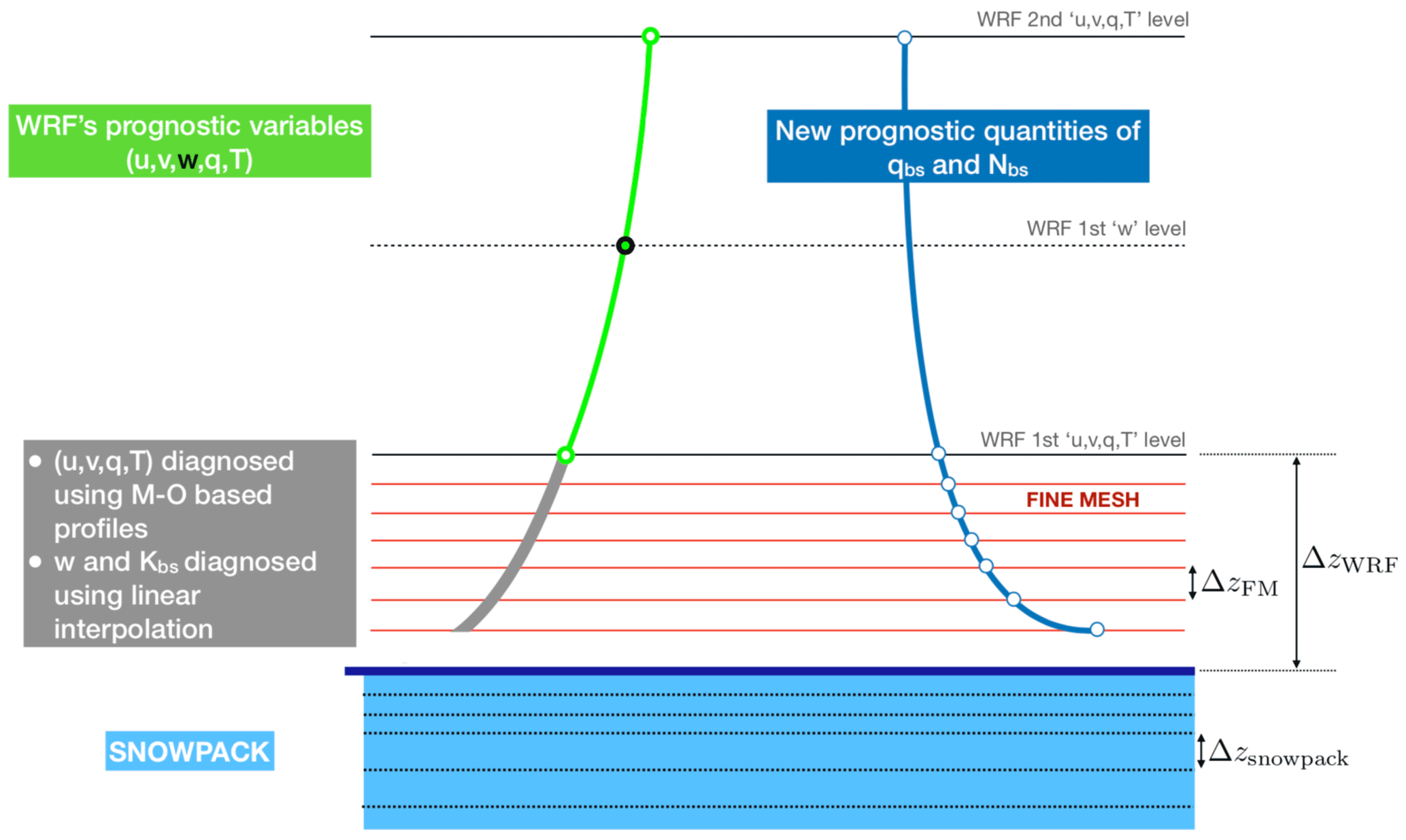
Figure 1 Vertical layering of the atmosphere and the snowpack. WRF's vertical mesh is staggered with vertical velocity (w) solved at mid-points (dotted black line) between the levels of the other prognostic variables (solid black line), such as horizontal velocities (u,v), temperature (T), and water mixing ratios (q). Numerical nodes lying on the solid black line are also called mass points. The new prognostic variables for blowing snow (q_bs, N_bs; blue profile) are solved on mass points and, additionally, on a newly introduced fine mesh (in red). On the fine mesh, the prognostic variables (u, v, q, T) are diagnosed using Monin–Obukhov similarity theory (grey section of the green vertical profiles). Vertical velocity (w) and the turbulent diffusion coefficient (K_bs) are linearly interpolated between the surface and first w level. Δz_FM indicates the vertical layer thickness of the fine mesh (FM), Δz_WRF indicates the layer thickness of the first WRF model level, and Δz_SNOWPACK shows the layer thickness of the SNOWPACK model layers.

The equation for q_bs is spatially discretized to cell centres of the Arakawa C grid, which are referred to as mass points in WRF's terminology. These are the same grid points at which various prognostic scalars such as temperature, moisture and other hydrometeors are defined. The vertical discretization is illustrated in Fig. 1. As shown in this figure, there is an additional fine-resolution mesh uniquely for the blowing snow variables between the surface and the first WRF mass point level. The additional fine mesh (FM) is required because the blowing snow variables have extremely large gradients in the vertical, compared to other scalars (e.g. temperature), because of the impact of sedimentation. In mesoscale models such as WRF, the first model level above the surface, Δz_WRF, is ∼𝒪 (10 m), which is far too coarse to capture the sharp gradients near the surface. The fine mesh has a mesh size, Δz_FM is ∼𝒪 (1 m), with the first FM level fixed to 50 cm above the surface. The number of levels in the fine mesh can be chosen at runtime and remains fixed during the simulation. Typically, 8 to 10 levels are sufficient to capture the near-surface gradients. Values for WRF's prognostic variables are diagnosed for points on the fine mesh using either the stability-corrected log laws (u, v, T, q) or a simple linear interpolation (w and K_bs). The implementation of the FM in CRYOWRF is inspired by SURFEX (Vionnet et al., 2012). In SURFEX, there is a prognostic, multi-layer surface layer scheme called CANOPY (Masson and Seity, 2009), whereas in the current version of CRYOWRF, the values of the atmospheric variables are only interpolated onto the fine mesh.

To follow WRF's existing framework to solve for hydrometeors, we begin by reformulating Eq. (1a) as follows:

$$\begin{array}{}\text{(20)}& {\displaystyle \frac{\partial q_{\mathrm{bs}}}{\partial t}}={\left[{\displaystyle \frac{\partial q_{\mathrm{bs}}}{\partial t}}\right]}_{\mathrm{m}+\mathrm{s}}+{\left[{\displaystyle \frac{\partial q_{\mathrm{bs}}}{\partial t}}\right]}_{\mathrm{p}}+{\left[{\displaystyle \frac{\partial q_{\mathrm{bs}}}{\partial t}}\right]}_{\mathrm{advec}},\end{array}$$

where the three terms (from left to right) on the right-hand side of the above equation are contributions from turbulent mixing and sedimentation (m+s), phase change (p), and advection (advec), respectively. They are stated as follows:

$$\begin{array}{}\text{(21a)}& {\displaystyle }{\left[{\displaystyle \frac{\partial q_{\mathrm{bs}}}{\partial t}}\right]}_{\mathrm{m}+\mathrm{s}}& {\displaystyle }=-K_{\mathrm{bs}}{\displaystyle \frac{{\partial }^{\mathrm{2}}{q}_{\mathrm{bs}}}{\partial x_i^{\mathrm{2}}}}{\mathit{\delta }}_{i\mathrm{3}}+{\displaystyle \frac{\partial }{\partial x_i}}\left(q_{\mathrm{bs}}{V}_q{\mathit{\delta }}_{i\mathrm{3}}\right)\text{(21b)}& {\displaystyle }{\left[{\displaystyle \frac{\partial q_{\mathrm{bs}}}{\partial t}}\right]}_{\mathrm{p}}& {\displaystyle }=S_q\text{(21c)}& {\displaystyle }{\left[{\displaystyle \frac{\partial q_{\mathrm{bs}}}{\partial t}}\right]}_{\mathrm{advec}}& {\displaystyle }=-u_i{\displaystyle \frac{\partial q_{\mathrm{bs}}}{\partial x_i}}.\end{array}$$

Equation (21a) is solved in a semi-implicit fashion (fully implicit for turbulent mixing and explicit for sedimentation), using second-order finite differencing, resulting in a tridiagonal matrix that is solved using the well-known Thomas algorithm. The semi-implicit matrix-based solver is required to make the solver numerically stable and able to deal with the fine resolution of the fine mesh and the relatively coarse resolution of WRF's native mesh in the same matrix. Immediately after, Eq. (21b) is solved in an explicit fashion for both the fine mesh and WRF's native mesh together. The heat and mass transfer quantities in the region of the fine mesh are added as correction terms to the first WRF level to ensure conservation of mass and energy. Equation (21c) is solved using WRF's existing advection routines for scalars, similar to how hydrometeors are advected. The possible advection algorithms in WRF range from finite difference schemes of different orders, and positive definite schemes to weighted essentially non-oscillatory (WENO)-type schemes, etc. Temporal integration of Eq. (21c) is done using second- or third-order Runge–Kutta. The numerical algorithms for the advection of blowing snow quantities is, at present, constrained to be the same as that for other scalars.

Finally, the mass balance at the surface due to precipitation and snow transport, Δm_sfc (kg m⁻² s⁻¹), is computed as follows:

$$\begin{array}{}\text{(22a)}& {\displaystyle }\mathrm{\Delta }{m}_{\mathrm{sfc}}=P+\underset{\mathrm{0}}{\overset{\mathrm{\infty }}{\int }}{\left[{\displaystyle \frac{\partial q_{\mathrm{bs}}}{\partial t}}\right]}_{\mathrm{m}+\mathrm{s}}{\mathit{\rho }}_{\mathrm{air}}\mathrm{d}z+{\mathrm{\nabla }}_H{Q}_{\mathrm{salt}},\text{where},\text{(22b)}& {\displaystyle }{\mathrm{\nabla }}_H={\displaystyle \frac{\mathrm{1}}{s}}\left({\displaystyle \frac{\partial u_{\mathrm{WRF}}}{\partial x}}+{\displaystyle \frac{\partial v_{\mathrm{WRF}}}{\partial y}}\right),s=\sqrt{u_{\mathrm{WRF}}^{\mathrm{2}}+v_{\mathrm{WRF}}^{\mathrm{2}}}.\end{array}$$

The first term on the right-hand side of the above equation is precipitation (P). The second term is the vertically integrated left-hand side of Eq. (21a) and represents the contribution of snow transport, specifically snow suspension. The final term, the horizontal divergence of saltation flux Q_salt, is the contribution of saltation to the surface mass balance. It is computed using the horizontal wind components at the first level of WRF (u_WRF,v_WRF) above the surface. The above formulation for surface mass balance is similar to that implemented in Alpine3D (Lehning et al., 2008).

2.4 Coupling library

A special coupling library was implemented to link SNOWPACK and WRF. This was necessitated by the fact that SNOWPACK is a C++ code base, and WRF, especially the physics routines, is largely written in FORTRAN. The coupling library has twin tasks. First, the coupler acts as an API that exposes SNOWPACK's C++ routines and makes them callable from FORTRAN codes. Second, as SNOWPACK follows the object-oriented programming (OOP) paradigm, and the coupling library allocates and maintains pointers to SNOWPACK objects during runtime.

The coupling library is written in a mixture of C++, C, and FORTRAN and consists of, for all practical purposes, two FORTRAN-callable subroutines, with one for initialization and one for a single time step execution. Thus, WRF maintains the time-stepping control, as is commonly the case for the interaction between an atmospheric model and the land surface model. Domain decomposition (MPI) and OpenMP-based loop parallelization are also organized by WRF's software framework, and therefore all computations within SNOWPACK's objects are serially executed.

The main design target for the coupling library was to ensure that it is agnostic of both the WRF and SNOWPACK versions. This is important because both code bases are under active development, and new versions with new or improved physical parameterizations or bugfixes are regularly released. The design target promises a long shelf life and thus ensures the viability of CRYOWRF in the future.

3 Model capabilities and performance

The overarching goal, while developing CRYOWRF from a usability perspective, was to make its adoption extremely simple for both new and experienced WRF users. This means that the entire workflow, beginning from the compilation of the model, the pre-processing, the actual simulation, and even to the post-processing of the results is ensured to be compatible with WRF, with only very minor changes from the standard process. Significant effort was also expended to ensure that CRYOWRF adopts all the capabilities of the parent WRF and SNOWPACK models. We list the most relevant of these capabilities below.

• Initialization. The snowpack is initialized through per pixel ascii files in the *.sno format. (This format is a standard format for SNOWPACK. For more details, see https://models.slf.ch/docserver/snowpack/html/snowpackio.html, last access: 3 December 2022). Helper Python scripts are provided to generate these files from the wrfinput files generated by running the WRF pre-processing programme real.exe that is a pre-requisite for running WRF.

• Restart. Once the model simulation has started, restarting the simulation (this is quite common for long simulations) is exactly the same as for the native WRF simulations. This is because all the relevant snowpack details, including depth profiles of snowpack quantities (snow temperatures, density, snow grain size, etc.), are stored in the wrfrst files.

• Input/output (IO). All snowpack outputs are managed by WRF's IO streams. This includes depth profiles and additional diagnostics such as terms for mass and surface energy balance.

• Nesting. CRYOWRF allows flexible launching of inner high-resolution nests. This is done by performing nearest-neighbour interpolation to initialize snowpacks in the inner nest from the coarser outer nest.

An additional capability is that the time step of SNOWPACK (Δt_SN) is flexible and can be any integer multiple of WRF's time step (Δt_WRF), as illustrated in Fig. 2. It is important to note that ice mass (blowing snow and precipitation) is exchanged between WRF and SNOWPACK at every Δt_WRF. This is particularly important to account for erosion/deposition due to blowing snow, as the blowing snow model is necessarily calculated at every WRF time step. At every (Δt_SN), the heat equation for snowpack, along with metamorphism, settling, and melt freeze of the snowpack layers are solved. The forcings from WRF are the incoming shortwave and longwave radiation along with temperature, relative humidity, wind speed, and SNOWPACK returns to WRF, the sensible and latent fluxes, and albedo and surface temperature. Note that, in the current model, the surface roughness length is kept fixed for glaciated pixels. Thus, the update for surface roughness length occurs only upon transition from non-glaciated to glaciated (typically upon snowfall), and vice versa (typically upon melt). The flexible time-stepping capability can be quite important as, depending on the settings used for SNOWPACK, many tens to hundreds of snow layers may have to be accounted for. For such cases, calling SNOWPACK at every time step would be prohibitively expensive, without significantly increasing the accuracy of the simulation from the atmosphere's perspective.

The computational costs of using SNOWPACK as a LSM scheme in relation to existing LSM models were assessed. A simulation domain with 64 × 64 surface pixels was chosen (it was ensured that each pixel in the domain is a land pixel, and no water pixels are found in the domain). A baseline simulation was performed using Noah-MP and compared with separate CRYOWRF simulations with 10, 50, 100, and 400 layers of snow, respectively. The number of layers was kept fixed during the course of these benchmarking simulations. For each CRYOWRF set-up, three variants were simulated. These were (i) with WRF and SNOWPACK time steps being equal (Δt_SN=Δt_WRF), (ii) the time step of SNOWPACK being 10 times that of WRF (Δt_SN=10Δt_WRF), and, finally, (iii) the same as the previous variant but with the blowing snow module switched off. An additional simulation with the Community Land Model (CLM) was also performed. Apart from changes in the LSM set-up, all the simulations had exactly the same set-up (WRF time step, radiation, boundary layer scheme, etc.) and were compiled with exactly the same compiler and compiler settings.

The results of these simulations are presented in Fig. 3, with percentage increase in runtime with respect to the Noah-MP baseline case chosen as the metric. For reference, it must be noted that Noah-MP and CLM use three and five snow layers, respectively. The first variant, with equal SNOWPACK and WRF time steps, scales (nearly linearly) the number of simulated snow layers, with a 30 % increase for 10 snow layers and increasing up to 240 % for 400 snow layers. From this perspective, there is indeed a significant overhead of using SNOWPACK as the LSM. The benefits of variable time-stepping for SNOWPACK are immediately clear when comparing the costs of the second variant. In this case, while there is an increase in runtime, it is not as significant, with a much lower (38 %) increase for 400 snow layers. For simulations with more reasonable numbers of snow layers, the computational costs are less than 15 %, which is higher than Noah-MP. To put SNOWPACK's computational overhead in perspective, the CLM model (being called at every time step), requires 84 % longer runtime. The overhead due to the blowing snow module is insignificant in all cases. This analysis proves that using an advanced-complexity snow model coupled to WRF is feasible from a performance perspective.

It is important to note that the capability of using different time steps for SNOWPACK and WRF is a choice provided to the user. This capability must be juxtaposed with the capability of SNOWPACK to simulate a constrained number of layers or snow height. Calling SNOWPACK at larger intervals would result in degrading the quality of surface fluxes while keeping the computational cost low. However, the larger time step would only be required if the goal of the study is to study the snowpack at very high vertical resolution, thereby necessitating hundreds of layers of snow. As described earlier, the goal of CRYOWRF is to be useful for simulations at vastly different spatial and temporal scales. The motivations for simulations at different scales are typically orthogonal. For example, one may choose to use CRYOWRF in a turbulence resolving large-eddy simulation (WRF-LES mode) to study snow–atmosphere interaction. In such a numerical experiment, it may be prudent to call SNOWPACK at every time step while simulating only a couple of snow layers. On the other hand, a user perhaps wants to perform continental-scale simulations for surface mass balance where it is imperative to use a large number of snow layers and where calling SNOWPACK at every time step is not necessary. Future studies using CRYOWRF in different experiments would ultimately result in coming up with a set of best practices for each case.

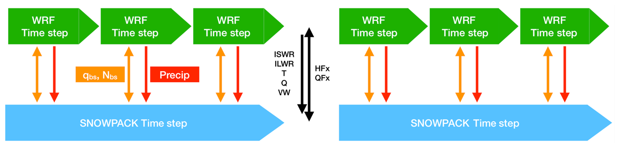
Figure 2 Flexible time-stepping of SNOWPACK within CRYOWRF. SNOWPACK can be called at any integer multiple of WRF's time step. In this schematic, SNOWPACK is called every three WRF time steps. The orange (blowing snow) and red (precipitation) arrows indicate fast exchange of mass between the snowpack and WRF. At intervals of Δt_SN, slow dynamics for thermal processes are accounted for by solving the heat equation in the snowpack.

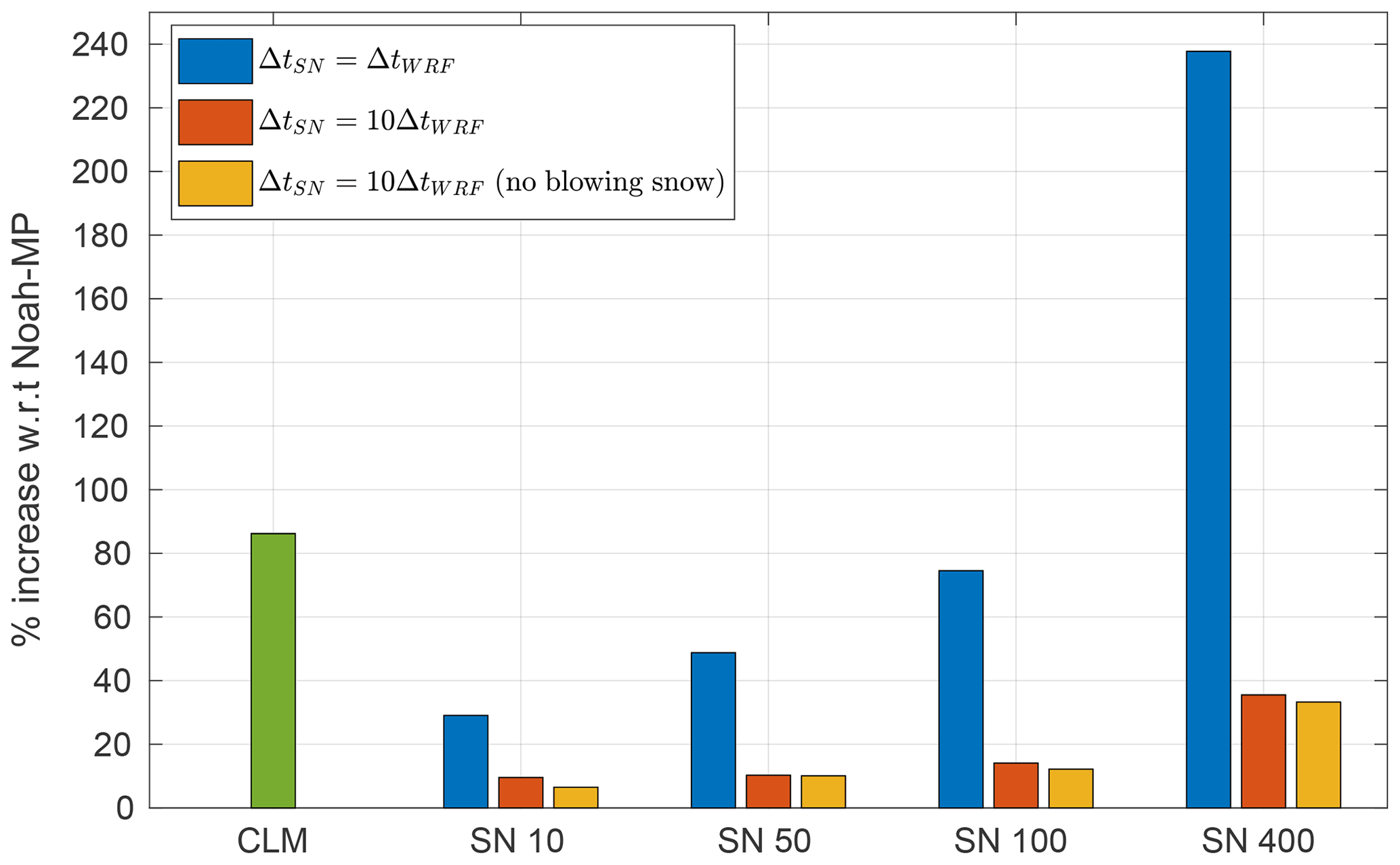
Figure 3 Runtime cost of CRYOWRF. Percentage increase in runtime due to increasing number of simulated snow layers. Number of snow layers simulated are 10, 50, 100, and 400 layers. The percentage increase is calculated with respect to a simulation with Noah-MP being treated as a baseline. An additional comparison with CLM model is also shown. Different coloured bars represent the computational overhead without (blue bars) and with SNOWPACK's variable time step (red bars), along with the overhead of simulating blowing snow (yellow bars).

4 Case studies using CRYOWRF

In this section, several case studies using CRYOWRF are presented. These case studies are primarily intended to showcase the breadth of scenarios that CRYOWRF can simulate at present. These scenarios range from continent-scale simulations, covering the entirety of Antarctica for climate-relevant studies, to a local, valley-scale simulation in Alps. Note that the presentation of the case studies does not go into detailed intercomparisons with measurements, etc. This is beyond the scope of this article and would be done in dedicated studies in the future. Thus, in the first case study, an intercomparison with data is presented to provide evidence of the model's accuracy, while the remaining results are presented directly from simulation outputs.

4.1 Case study Ia: continent-scale simulation of Antarctica for mass balance

4.1.1 Objectives

The first case study is a 1-year (July 2010–July 2011) simulation for the entire continent of Antarctica using CRYOWRF. The chosen simulation set-up is standard for mass balance calculations in Antarctica and comparable with the most common models of RACMO and MAR (e.g. Agosta et al., 2019). The intention of this case study is to demonstrate the accuracy of the CRYOWRF model along with showcasing the kind of information now available directly from CRYOWRF, particularly with respect to the snow cover. This, and the following case studies, also serves as tutorials to ease the adoption of CRYOWRF for interested researchers.

4.1.2 Simulation set-up

The simulation is performed over a single domain with a horizontal resolution of 27 km, covering the domain shown in Fig. 4. The domain encompasses the entire continent along with a substantial portion of the surrounding Southern Ocean. Static data (topography and land use) are from the 1 km resolution Reference Elevation Model of Antarctica dataset (REMA; Howat et al., 2019) and the AntarcticaLC2000 land use data (Hui et al., 2017), respectively, and were prepared as WRF input by Gerber and Lehning (2020). The model is initialized and forced at the lateral boundaries by ERA5 reanalysis data (Hersbach et al., 2020). The parameterizations used are RRTMG (Rapid Radiative Transfer Model; shortwave and longwave radiation), Kain–Fritsch (KF; convection), a modified version of the Morrison scheme that improves representation of secondary ice production (microphysics; Vignon et al., 2021; Sotiropoulou et al., 2021), and MYNN (Mellor–Yamada–Nakanishi–Niino; boundary layer scheme). The simulation is nudged against ERA5 for wind speeds in the zonal and meridional direction in the top 20 levels of the atmosphere. A total of 64 atmospheric levels are simulated with the topmost pressure level set at 10 kPa (approximately 15 km a.s.l. – above sea level). The lowest layer is on average 8 m a.g.l. (above ground level), and there are 22 layers within the first 1 km above the surface.

The land surface model (LSM) is the SNOWPACK model. The snow cover is initialized using data from Utrecht University's Firn Densification Model (FDM; Ligtenberg et al., 2011), forced by RACMO 2.3 (van Wessem et al., 2018), which provides vertical profiles for snow layer thickness, density, and temperature, along with grain radius for the entire continent. Pixel-wise ASCII files are created from the FDM data (which is in netcdf format). The simulation is initialized for only the top 20 m of the snowpack. Snow cover modelling requires parameterizations for many different processes. To calculate albedo, we used the model developed by Munneke et al. (2011) and implemented in SNOWPACK by Steger et al. (2017b). The new snow density is fixed to 300 kg m⁻³, and the water transport through a snow column is done using the bucket approach. Snow–atmosphere exchange of mass and energy is calculated using the Holtslag surface layer model (Schlogl et al., 2017). The snow surface roughness is fixed at 0.002 m. The minimum thickness of a snow layer is set to 0.001 m. This is indeed quite a small value and was chosen as such to simply demonstrate CRYOWRF's ability to model snowpacks at such extreme resolutions. The blowing snow model was active with an eight-layer fine mesh between the surface and the first mass point of WRF. The resolution of the fine mesh extended between 0.5 m (closest to the surface) and 1.5 m.

4.1.3 Atmospheric weather stations (AWSs)

Results of this simulation are compared to weather station measurements from 14 stations spread throughout the continent (mostly along the coast and marked in red in Fig. 4). Station data are taken from several databases. A summary is given in Table 1. No thorough quality checks were performed for the station data for this study. Data gaps are commonly occurring. Some stations provide no information about relative humidity (Mizuho), pressure (D-17), and wind direction (D-17). In addition to a verification with AWSs data, figures of the surface mass balance components and snow profiles showcasing the capabilities of the entire CRYOWRF framework (including diagnostics) are presented in the following section.

Lazzara et al. (2012)König-Langlo (2012)Amory (2020)

Table 1 Atmospheric weather stations used for model verification. Last access for all URLs: 3 December 2022.

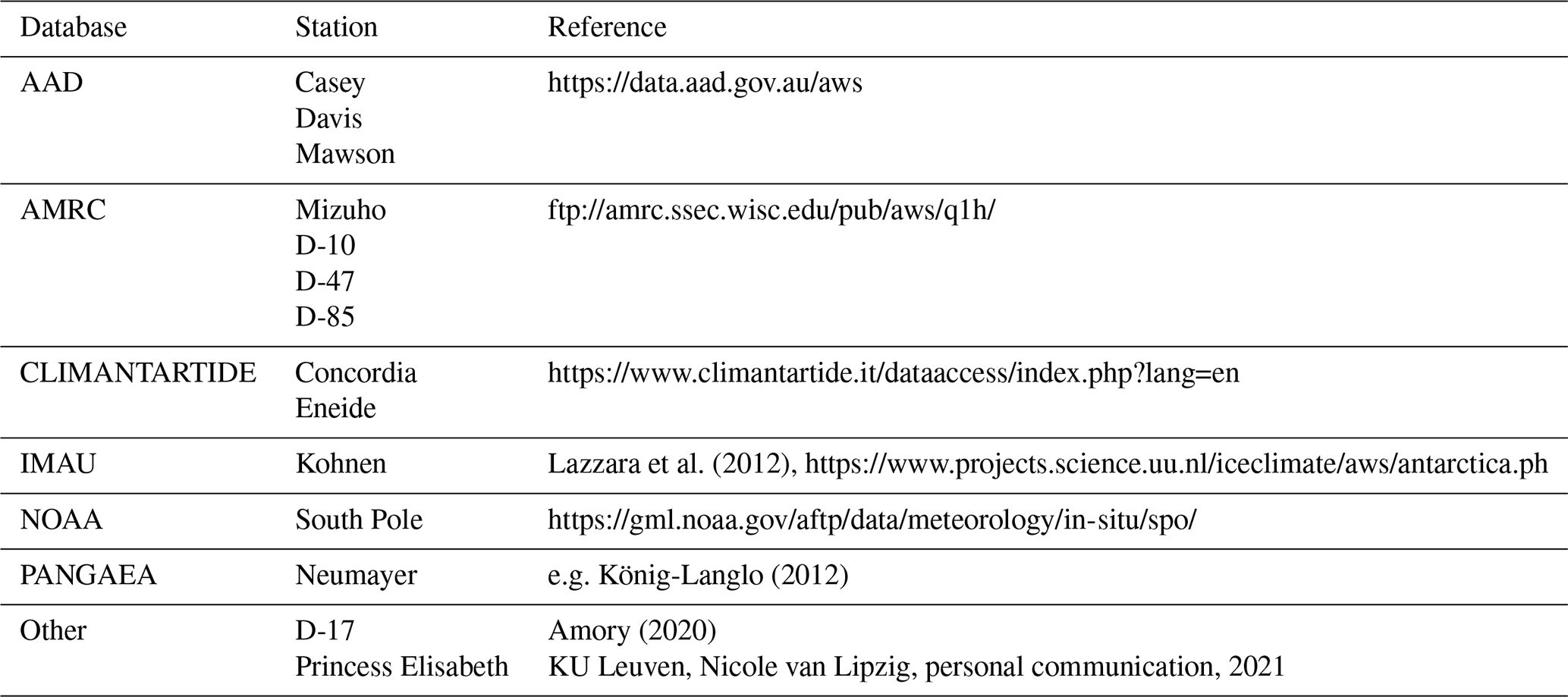
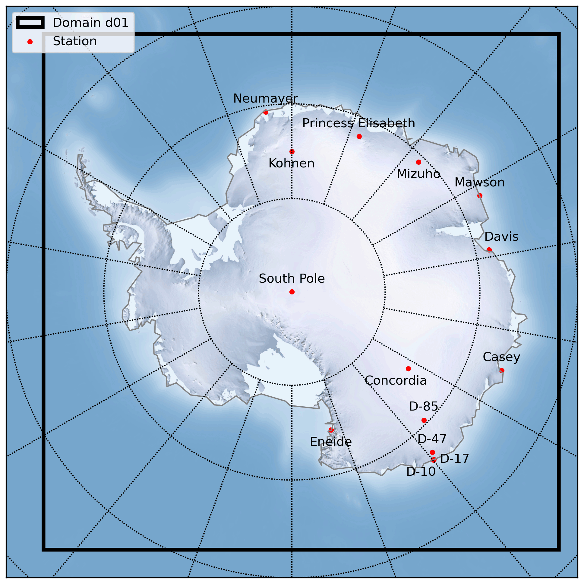
Figure 4 Simulation domain for case study Ia (black rectangle). The simulation domain encompasses the entire continent. Additionally, measurement stations used for model verification are represented by red dots.

4.1.4 Results

Figure 5 shows scatterplots comparing the measurements (on the horizontal axes) with CRYOWRF outputs (on the vertical axes) for the four standard meteorological variables of surface pressure, potential temperature, and relative humidity (with respect to ice) at 2 m above surface and wind speed at 10 m above surface. For comparison, results from a simulation with Noah-MP as the LSM are also shown. The best correlation is found for surface pressure (r=0.90) and the worst correlation for relative humidity (r=0.31), with CRYOWRF outperforming or being similar to Noah-MP for each of the variables. Though, admittedly, the improvements over Noah-MP are minor, except for relative humidity.

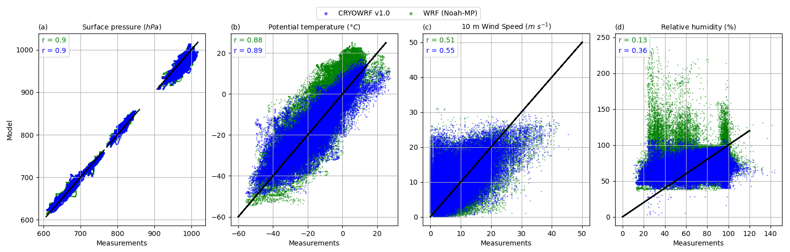
Figure 5 Correlation plots between CRYOWRF time series output (blue) and measurements. All measurements are consolidated. For comparison, results with Noah-MP are shown (green). The correlation results are presented for surface pressure (a), 2 m potential temperature (b), 10 m wind speed (c), and 2 m relative humidity (d).

The South Pole was chosen to present an example of direct comparison of time series between CRYOWRF, Noah-MP, and measurements. These are shown in Fig. 6. In addition to time series, a comparison of the probability density functions (PDFs) for the entire time series is shown in adjoining figures on the right for each row. In addition to the four variables presented earlier, wind direction time series are shown as well. It is clear that CRYOWRF follows the measurements reasonably well. Additionally, CRYOWRF performs better than Noah-MP with lower mean absolute errors (mae), for each variable. The best improvement is found for potential temperature and relatively humidity. The same conclusions can be drawn from the PDF plots. For example, the PDFs of CRYOWRF and measurements of potential temperature have much overlap in comparison to that with Noah-MP, which has a significant warm bias. The improvement in CRYOWRF with respect to Noah-MP could be due to a multitude of reasons. A recent study by Xue et al. (2022), for example, attributed the warm bias in Noah-MP to low albedo. Another reasoning, for example, could be that CRYOWRF includes the effect of blowing snow sublimation, which has a cooling effect on the atmosphere. Finally, measurements, especially of variables such as relative humidity at extremely low temperatures, are known to be unreliable. However, all this is mere speculation, and a deeper analysis would be necessary to explain these differences, which is beyond the scope of this study. At the very least, Figs. 5 and 6 show that CRYOWRF produces comparable results to Noah-MP out of the box.

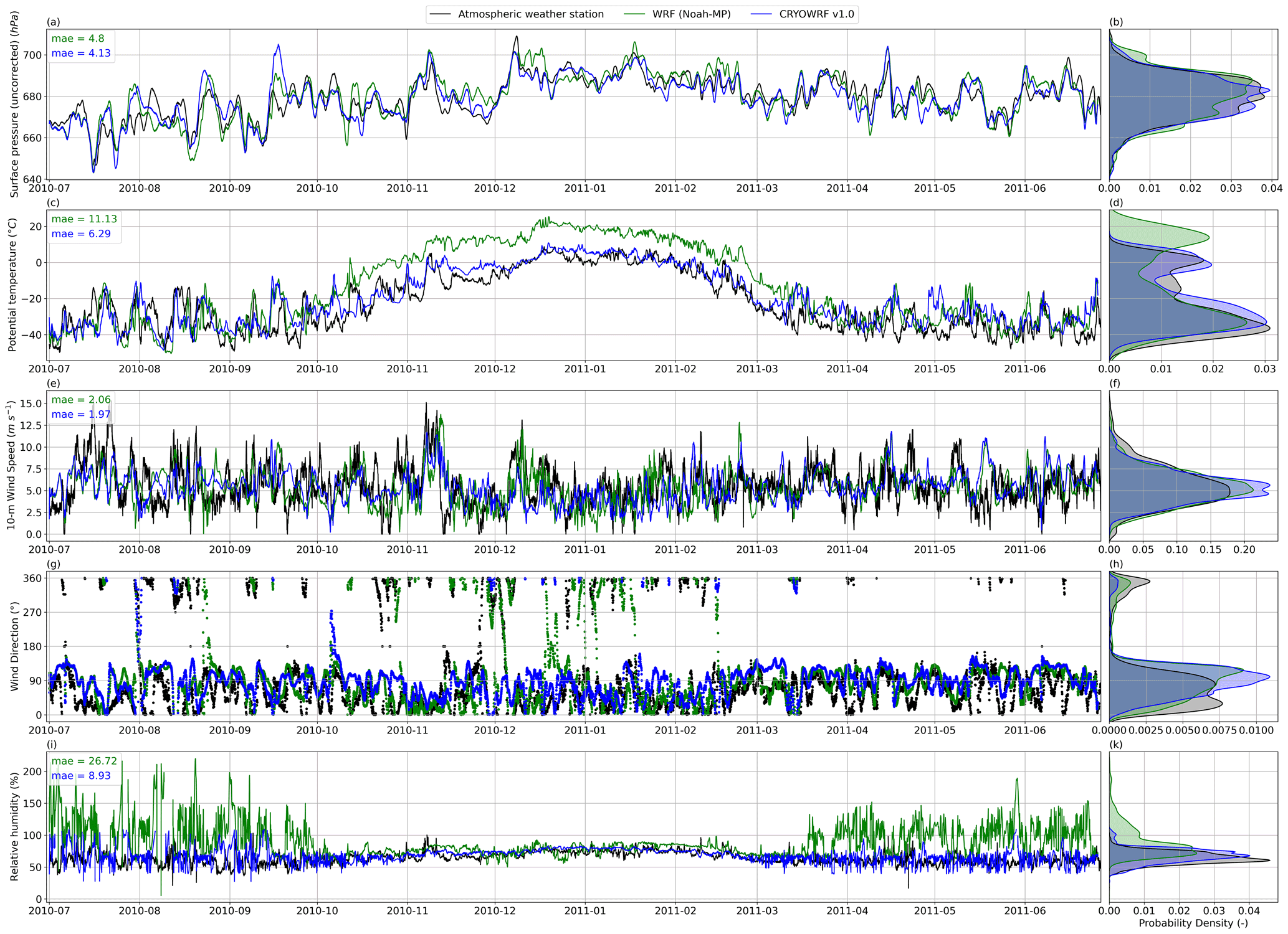
Figure 6 Time series comparison between CRYOWRF, Noah-MP, and measurements using the automatic weather station at the South Pole for surface pressure (a), 2 m potential temperature (c), 10 m wind speed (e), wind direction (g), and relative humidity (with respect to ice) (i). The distributions of these quantities over a period of 1 year are shown in the adjoining figure on the right in each row (b, d, f, h, k).

One major reason for performing simulations such as in this case study is to calculate components of the surface mass balance (SMB). The polar surface mass balance is of critical importance in understanding the implications of global warming on sea level rise. CRYOWRF outputs these quantities as two-dimensional fields directly as a part of the standard output via its specially implemented diagnostics package. An example of the surface mass balance output during this case study is shown in Fig. 7. Since the simulation period is of only 1 year, it is not possible to quantitatively compare the results presented in this figure with those published in the literature, which are typically calculated over climate timescales of at least 30 years. In fact, given the interannual variability in SMB patterns, particularly at the coast (due to phenomena such as atmospheric rivers), it is likely that the numbers from 1 year, as shown in Fig. 7, may be different from long-term averages. However, qualitatively, the spatial patterns for each of the different terms matches quite well (for example, Agosta et al., 2019). For example, precipitation is dominant in west Antarctica and the peninsula, while in east Antarctica, it is limited to the coasts, with strong gradients along the topographic contours. It is interesting to see melt–refreeze dynamics being dominant in the Ross and Ronne ice shelves. Sublimation (or vapour deposition) patterns reveal the importance of this mechanism on the coastline, while identifying locations in the interior of the continent where vapour deposition is actually a net positive term in the surface mass balance.

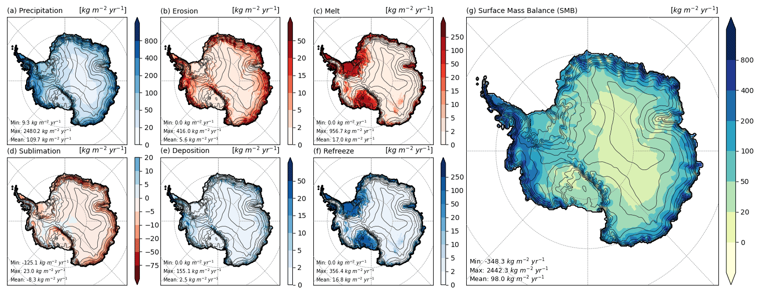
Figure 7 Components of the surface mass balance output directly from CRYOWRF.

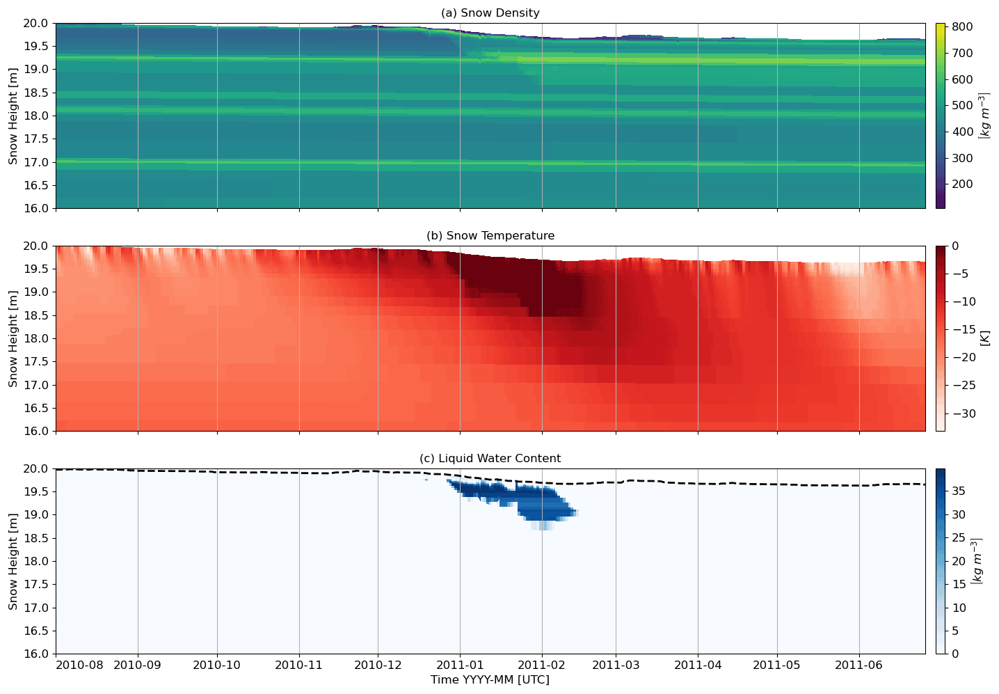
Figure 8 Profiles of snow density (a), temperature (b), and liquid water content (c) at the Casey station (66.4058^∘ S, 110.8043^∘ E) simulated by CRYOWRF for the duration of the 1-year simulation between August 2010 and June 2011.

A notable feature of CRYOWRF is its ability to run atmospheric simulations with highly (vertically) resolved snowpacks. This allows an accurate representation of thin subsurface ice layers with a thickness of the order of a few millimetres that have significant impact on snow hydrology at larger scales (Wever et al., 2016b). In Fig. 8, the evolution of the snowpack at the Casey station (66.4058^∘ S, 110.8043^∘ E) on the eastern Antarctic coastline is represented by the density, temperature, and liquid water content (LWC) profiles. For this location, based on the local mass and thermal forcing, SNOWPACK converges to 130 snow layers. As can be seen in the density profiles, thin layers of high-density snow (or ice) layers can be found within the top 1 m of the snowpack. These layers are mostly less than 1 cm thick and are between layers of (in some cases, considerably) lower density. The top 1 m of the snowpack is also thermally active, with significant cooling/warming at the diurnal and seasonal scale, relative to subsurface temperature fluctuations. The exceptional period is between the middle of December till the middle of February when significant melt occurs, reducing by nearly 0.5 m of snow. The meltwater percolates through the snowpack up to a depth of 1 m, resulting in isothermal melting point temperatures at the beginning of February. The meltwater percolation is clearly seen in the LWC profiles, where significant meltwater is found to remain in a localized region at the depth of 1 m until the middle of February.

4.2 Case study Ib: multiscale simulation at Dumont d'Urville – formation of hydraulic jumps

4.2.1 Objectives

The second case study simulates the formation of an hydraulic jump at the coast surrounding the Dumont d'Urville (DDU) station between 8 and 11 August 2017. The hydraulic jump occurs when a well-developed, high-velocity katabatic flow draining off the sloped ice sheet of Antarctica reaches the coast. The high-velocity outflow experiences an abrupt and rapid transition due to changes in topographic and surface conditions, thereby transitioning to a hydraulic jump. The hydraulic jump itself further triggers gravity waves. A remarkable manifestation of the hydraulic jump, given the right surface conditions, is the large-scale entrainment and convergence of blowing snow particles within the hydraulic jump. This can result in the formation of 100–1000 m high, highly localized walls of snow in the air in an otherwise cloud-free sky.

The case study is directly inspired by the recent work of Vignon et al. (2020), who present a detailed analysis on the genesis, dynamics, and implications of the hydraulic jumps and the corresponding gravity waves in the region in proximity of DDU. Their study used (standard) WRF as the principal tool and showed that capturing this phenomenon in simulations is only possible with high-resolution domains with resolutions higher that 3 km at the very least.

This case study serves as a perfect example to highlight the capabilities of CRYOWRF both from a physical modelling and a technical perspective. CRYOWRF, due to its non-hydrostatic atmospheric core can indeed simulate such a phenomenon, in direct contrast with the pre-eminent mesoscale models for polar research, namely RACMO and MAR. From a technical perspective, performing such a simulation necessarily requires a nested domain approach. As mentioned earlier, CRYOWRF is compatible with the nesting capability of WRF. Finally, unlike Vignon et al. (2020), who used standard WRF, CRYOWRF includes the blowing snow model, which allows for studying the impact of hydraulic jump formation on blowing snow dynamics and simulating the formation of the aforementioned snow walls for the first time.

4.2.2 Simulation set-up

The simulation set-up is as follows: a three-domain simulation is performed, having horizontal resolutions of 12 km (d01), 4 km (d02), and 1 km (d03) for the three domains. All the domains are centred on DDU, with the Adélie Land coastline approximately passing diagonally across the domains. The domain locations and extents are shown in Fig. 9. The nesting is of a one-way nature, i.e. the inner, higher-resolution domain is forced at the lateral boundaries by the outer, coarser domain, while there is no upscaling of the inner domain data to nudge the outer domain. The outermost domain (d01) has exactly the same set-up as that in the previous case study (apart from the resolution), i.e. the same static data and physical parameterizations are used, and ERA5 is used to force the simulations. The two inner domains also have the same set-up as the outer domain, with the exception that the convection parameterization is switched off. The blowing snow model is active in all three domains. The three domains have 69 vertical levels in the atmosphere, with top-level pressure fixed at 5 kPa (approximately 18 km a.s.l.). Similar to the previous set-up, the lowest layer is on average 8 m a.g.l., and there are 22 layers within the first 1 km above the surface.

The simulation starts with only the outermost domain first, with the inner domains activated successively. The snow profile at each of the pixels is initialized using *.sno files generated from a restart (wrfrst) file from a coarse-resolution simulation, similar to that in case study Ia. The starting times for the three domains are the 8 August 2017 at 00:00 and 06:00 UTC and 9 August 2017 at 00:00 h for the three domains, respectively. The simulation of all three domains continues until 11 August 2017. Increasing resolution implies decreasing time steps. The three domains used time steps of 45, 15, and 5 s, respectively. The LSM (SNOWPACK) uses a time step of 900 s in each of the three domains, using the built-in capability of CRYOWRF to call the LSM module with flexible time steps. Using a lower time step for the LSM is justified, since the phenomenon we are interested in simulating is a purely mechanical one and not particularly dependent of the near-surface heat fluxes, thermal snow–atmosphere interaction, and certainly not the surface and subsurface thermodynamics.

In the following section, two illustrations of model output are shown where the hydraulic jump and the excited gravity waves, along with its effect on blowing snow, can be seen. Differences between the domains on account of the resolution are also highlighted.

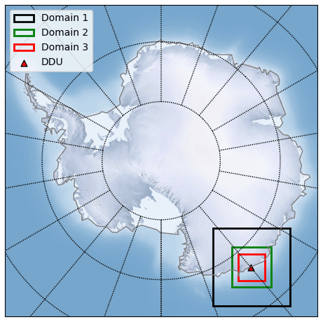
Figure 9 Simulation domains for case study Ib (coloured rectangles). The three nested domains of 12 km (black), 4 km (green), and 1 km (red) resolution. These domains are centred at the Dumont d'Urville (DDU) station (red triangle).

4.2.3 Results

As reported by Vignon et al. (2020), using station measurements, there is a relatively quiescent period before the 9 August 2017, with stable wind speed, wind direction, and air temperature recorded at DDU. The situation dramatically changes on the 9 August when the katabatic flow rapidly strengthens, and very high wind speeds are reported at DDU in the first half of 10 August. At 12:00 UTC on 10 August, there is a sudden drop in the wind speed, following which the wind becomes gusty but on average remains slower than the previous day. Vignon et al. (2020) showed that the abrupt deceleration of the katabatic flow is due to excitation of gravity waves and the enhanced friction induced.

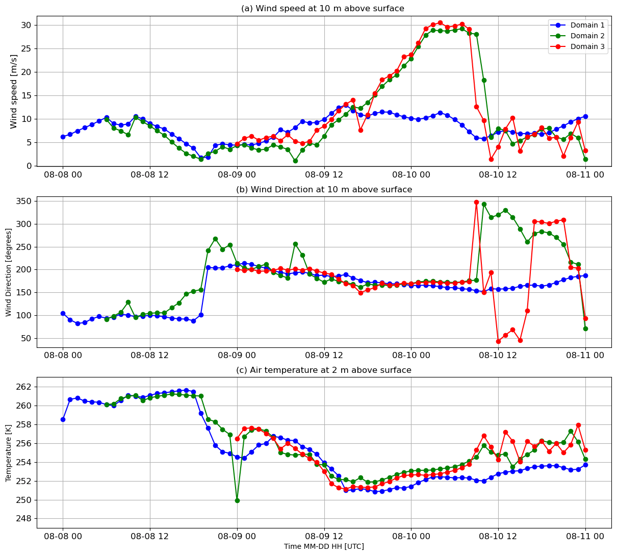
Figure 10 Meteorology at Dumont D'Urville as simulated by CRYOWRF. (a) Wind speed, (b) wind direction at 10 m above surface, and (c) air temperature at 2 m above surface.

These trends are reproduced by CRYOWRF and shown in Fig. 10, where the simulated time series of wind speed, direction, and temperature at the DDU station are plotted. It is interesting to note the differences in the trends shown by the three nested domains with different resolutions, particularly for wind speeds and direction. The coarse-resolution domain 1 (12 km resolution) follows the trends mentioned earlier, but the rate of wind acceleration and its abrupt slowdown are significantly less pronounced than the finer-resolution nests, which match each other quite well. Differences between the two inner nests emerge in the case of wind direction, where the flow in domain 3 shows significant oscillations in flow direction in the period before and after 12:00 UTC on 10 August. The flow direction resolved at 12 km resolution in domain 1 remains relatively fixed, on the other hand. The air temperature, initially quite stable on 8 August experiences a rapid decrease that coincides with the change in wind direction and an acceleration of wind speeds. This decrease continues until the middle of 9 August, followed by a warming trend. Interestingly, both the inner, higher-resolution domains are slightly warmer during the katabatic phase and at the onset of the gravity wave excitation, where temperature oscillations can be observed. These plots perfectly highlight the need for CRYOWRF's high-resolution capability because the intensity of the katabatic jet, its sharp transition into a hydraulic jump, can only be resolved by increasing the resolution from 12 to 4 km. The further phenomenon of gravity wave excitation is only possible by increasing the resolution even further to 1 km (Vignon et al., 2020).

The impact of the flow transitions on blowing snow dynamics are illustrated in the following two figures. Figures 11 and 12 both show the blowing snow mixing ratio q_bs (kg kg⁻¹) on 10 August 2017 at 12:00 UTC, for each of the three domains. This time period was chosen as the onset of gravity waves occurs close to this time (based on Fig. 10). Blowing snow at 1500 m a.g.l. is shown in Fig. 11, with DDU marked on the map (red triangle) along with the coastline (black line) for reference. In all three domains, there is a boundary delineating the regions with and without blowing snow. The boundary is precisely the location of the hydraulic jump. The effect of the model resolution is also clearly apparent. In the coarsest domain (domain 1; Fig. 11a), particle concentrations are lower and more uniformly spread. Increasing the resolution from 12 to 4 km, the concentration values increase, while at the same time, the part of the domain where blowing snow particles exist at this height shrinks to a smaller area as compared to the outer domain. Finally, in the innermost 1 km resolution domain, there is a clear imprint of wave-like fluctuations on the blowing snow concentration field. Vertical cross sections of the blowing snow mixing ratio are extracted at the dashed red line passing through DDU and are shown in Fig. 12. Additionally, potential temperature isotherms for values between 260 and 290 K are shown to indicate the presence of gravity waves. Similar to the previous figure, the flow in each of the three domains shows the characteristic hydraulic jump approximately 25 km inland from the coast. As expected, increasing the resolution results in a sharper localization of the jump location. Further inland from the coast, a thin region with high concentration of blowing snow particles can be observed. These particles are entrained into the hydraulic jump and are mixed up to much greater altitude off the coast. High concentrations are found even at 2000 m a.s.l. Only the innermost 1 km resolution nest exhibits signs of gravity wave excitation, as evidenced by the wavy perturbations to the isotherms, and particularly those for 270 and 280 K. Correspondingly, spatial patterns of the blowing snow mixing ratio matches the envelopes of the wave trains at different altitudes quite well. A video that shows the dynamics of the blowing snow mass mixing ratio for the entire simulation period is provided as Video M1 in the Supplement. This video shows the impact of the acceleration of the katabatic flow on blowing snow dynamics, the formation of the hydraulic jump, and the excitation of the gravity waves in the innermost 1 km domain.

This case study requires further detailed verification and analysis, even though, qualitatively, it reproduces satellite and visual observations of snow walls reported at DDU (see Vignon et al., 2020, for more data sources). More pertinent for the scope of this article is that this case study showcases an example of how CRYOWRF can contribute to enquiries in coupled snow–atmosphere interaction in polar regions that necessarily require high resolution. Extensive blowing snow clouds, with particles regularly reaching as high as 500 m above the surface, have been observed in satellite measurements (Palm et al., 2017) that have not yet been accurately simulated by models. High-resolution simulations of the sort presented in this case study may be useful in matching or explaining the satellite measurements and analyses of Palm et al. (2017).

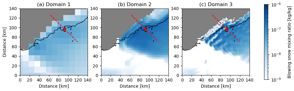
Figure 11 Blowing snow mixing ratio. Horizontal cross sections at 1500 m a.g.l. on 10 August 2017 at 12:00 UTC for the three domains with (a) 12 km, (b) 4 km, and (c) 1 km resolution. The red triangle indicates the location of the DDU station. The dashed red line indicates the location of the vertical cross section shown in Fig. 12. Note that the colour bar is logarithmic.

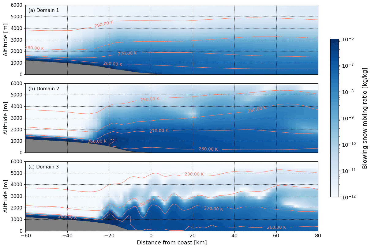
Figure 12 Blowing snow mixing ratio. Vertical cross sections at the transect through DDU indicated by the dashed red line in Fig. 11 on 10 August 2017 at 12:00 UTC for the three domains with (a) 12 km, (b) 4 km and (c) 1 km resolution. Four potential temperature contours are indicated (orange). Note that the colour bar is logarithmic.

4.3 Case study II: valley-scale simulation of a snow storm in the Swiss Alps

4.3.1 Objectives

This case study showcases the ability of CRYOWRF to simulate alpine snowpacks in complex topography. It highlights the ability of CRYOWRF (on account of its WRF-based atmospheric core) to perform extremely high-resolution, LES-scale snow–atmosphere coupled simulations in addition to mesoscale flows using the same modelling framework. Due to the differences in spatial and temporal scales relevant for alpine meteorology, as compared to polar meteorology, different snow physics parameterizations with higher precision are required for simulating alpine snowpacks compared to polar snowpacks. For example, this case study uses a different albedo parameterization than the previous, polar-based simulations. Meltwater dynamics, new snow density parameterization, and snow–soil interaction are additional examples of processes that are more crucial in alpine environments as opposed to polar regions. This case study thus provides an additional template for interested future users of CRYOWRF in terms of name list settings for SNOWPACK and WRF, which is more suitable for alpine environments.

In terms of novelty, the most interesting meteorological feature of this case study is the simulation of blowing snow in the Alps. While blowing snow in the Alps received significant attention in the cryospheric community from the surface mass balance (Vionnet et al., 2014; Gerber et al., 2018; Voegeli et al., 2016) and avalanche forecasting (Lehning and Fierz, 2008) perspective, its impact on different atmospheric components such as cloud dynamics or local radiative balance are unknown. There is evidence of potential feedback loops between blowing snow and cloud formation (Geerts et al., 2015; Vali et al., 2012). However, to the best of our knowledge, it has not been explored numerically.

4.3.2 Simulation set-up

The simulation consists of two domains, with the larger domain at a spatial resolution of 1.25 km, covering an area of 225 km², and the inner nest with a spatial resolution of 250 m, covering an area of 60 km². The outer domain covers a significant portion of eastern Switzerland and the adjoining parts of Austria and Italy, with the alpine arc passing roughly across the middle of the outer domain. The alpine town of Davos is located in the southwestern quadrant of the inner domain, offset by less that 5 km from the domain centre. The location of the domains and the complex topography over which the simulation is conducted are shown in Fig. 13. A total of 90 atmospheric levels are simulated, with the top-level pressure imposed at 15 kPa (approximately 11 km a.s.l). The lowest layer is 20 m a.g.l, with a total of 10 layers below 1000 m a.g.l.

The simulations performed are similar to those by Gerber et al. (2018) in that they are driven by hourly analyses fields of the operational COSMO model (COSMO refers to COSMO-1 in this study). Underlying topography and land use are from the Aster 1 s digital elevation model (NASA/METI/AIST/Japan Spacesystems and U.S./Japan ASTER Science Team, 2019) and the Coordination of Information on the Environment (CORINE) dataset (European Environmental Agency, 2006), respectively, prepared as WRF input as in Gerber and Sharma (2018). The difference is the use of CRYOWRF in this case study as opposed to standard WRF by Gerber et al. (2018). The boundary scheme in both domains is the Shin–Hong scale-aware scheme (Shin and Hong, 2015), which is applicable for resolutions as high as 250 m. This is a unique scheme in the WRF physics suite that is able to represent subgrid-scale mixing in the grey zone that exists between mesoscale flow 𝒪 (1 km) and turbulent flow 𝒪 (10–100 m). RRTMG is used for the parameterization of radiative effects both for short and longwave radiation, while the Thompson microphysics scheme is used to account for clouds. At the relatively high resolutions used in this case study, no convection scheme is required.

As mentioned earlier, using SNOWPACK as the LSM requires per pixel *.sno files for initializing the snowpacks at each pixel. In this case study, snow profiles are generated using snow height and snow density information from the single-layer data available in COSMO analysis fields and using 30 snow layers. The temperature of the layers is calculated via linear interpolation between the surface temperature and the underlying soil temperature, again using data from the COSMO fields. The initial grain diameter is arbitrarily chosen to be 300 µm, with bond diameters of 75 µm for all layers. The main difference between this case study and those presented earlier is that the underlying soil column is accounted for as well, with an additional 10 soil layers for each pixel. This is possible using SNOWPACK's existing capability for solving for both the soil and snow columns and is crucial for using CRYOWRF for simulating seasonal snow covers and over regions with partial snow coverage.

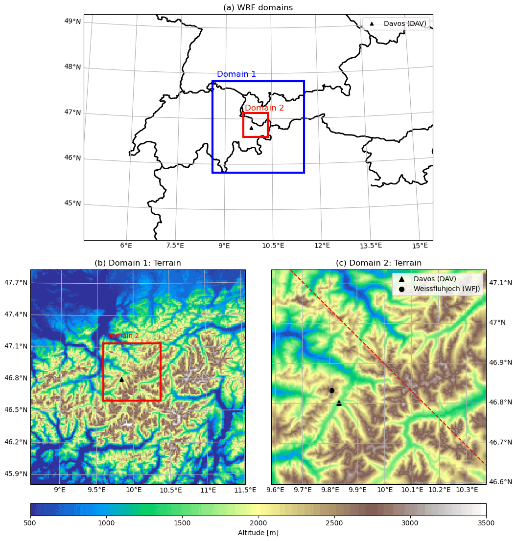
Figure 13 Location of the nested simulation domains for case study II. (a) Extent of the WRF domains with the location of Davos (DAV) shown (black triangle). (b, c) Underlying topography of the two domains, respectively. The red dashed line across the domain in panel (c) is the location of the along-wind cross-sectional view in Fig. 17 and Video M2 in the Supplement.

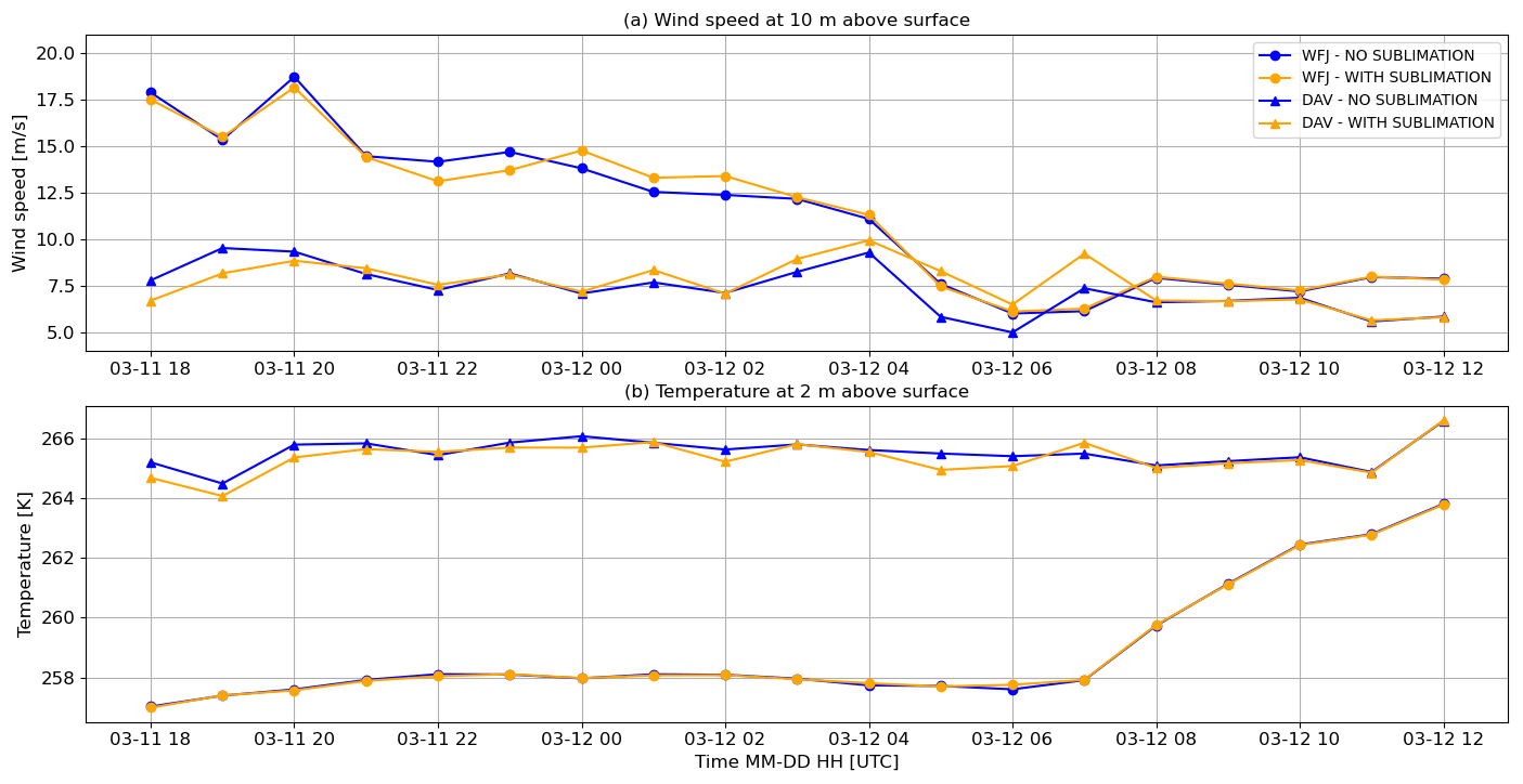
Figure 14 Time series of wind speed and air temperature, as simulated by CRYOWRF at Weissfluhjoch (WFJ) and Davos (DAV), between 11 March 2019 at 18:00 UTC and 12 March 2019 at 12:00 UTC.

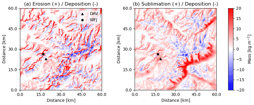
Figure 15 Impact of blowing snow. (a) Erosion and deposition of snow at the surface due to snow transport. (b) Sublimation (or deposition) of blowing snow particles in the atmosphere. Stations DAV and WFJ are marked by a black triangle and circle, respectively.

4.3.3 Results

The above simulation was performed for a period of 36 h, beginning on 11 March 2019 at 00:00 UTC for the inner, high-resolution domain. This period is coincident with a period with high wind speeds recorded on alpine ridges surrounding Davos. Furthermore, the wind direction is from the northwest, blowing across the inner simulation domain, such that many of the ridges simulated in the region are nearly perpendicular to the dominant, large-scale flow direction. After allowing for an extensive period for the spin-up of the model, results are analysed only for the period between 18:00 UTC on 11 March 2019 and 12:00 UTC on 12 March 2019.

To set the meteorological context of the case study, wind speed and temperature simulated by CRYOWRF at two locations, the upper, Weissfluhjoch station (denoted as WFJ; 46.833323^∘ N/9.806371^∘ E; altitude of 2691 m a.s.l.) and at Davos (denoted as DAV; 46.802128^∘ N/9.833477^∘ E; altitude of 1594 m a.s.l.) in the valley (is shown in Fig. 14). Two variants of the simulation, with and without blowing snow sublimation, were performed to assess the impact of enhanced heat and mass transfer between the particles and the atmosphere. The wind speed within the valley is reasonably stable and moderate, with values of approximately 7.5 m s⁻¹. On the other hand, at high altitudes, the wind is significantly faster at 18:00 UTC, reaching speeds as high as 20 m s⁻¹ at WFJ. The wind speed at WFJ decelerates from this high value but remains significantly higher than those in the valley until 04:00 UTC on 12 March. As expected, the air temperature is lower at WFJ than at DAV initially, and the higher-altitude regions experience significant warming on 12 March 2019.

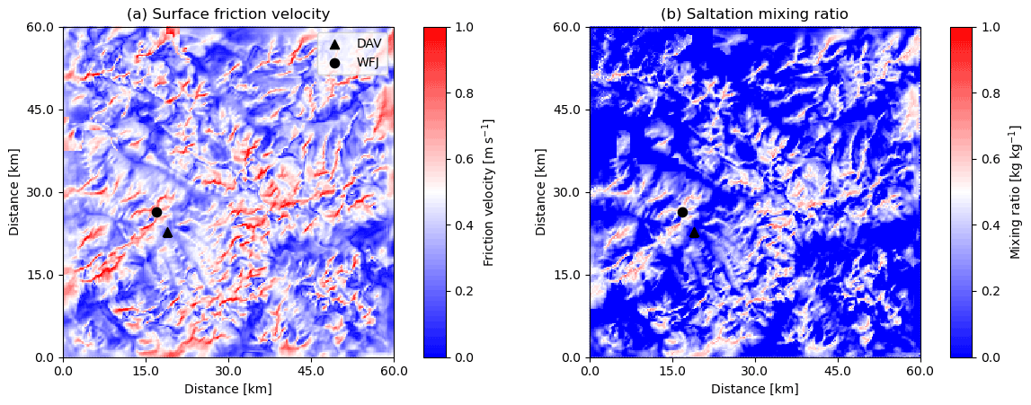
Figure 16 Modelling of snow transport. (a) Surface friction velocity that triggers saltation. (b) Mixing ratio of blowing snow in the saltation layer. Stations DAV and WFJ are marked by a black triangle and circle, respectively. Results shown are at 00:00 UTC on 12 March 2019.

Figures 15 and 16 present surface maps of various diagnostic quantities relevant for blowing snow dynamics calculated in the innermost, 250 m resolution domain. In Fig. 15a, patterns of cumulative erosion and deposition during the course of the simulation are shown. It is instructive to compare the regions of extensive blowing snow erosion and deposition with the topography in Fig. 13c. The most active areas for snow transport are the ridges perpendicular to the flow as expected. It can be observed further that erosion occurs mostly on the windward side of the ridges, with zones of deposition found immediately on the leeward side, which is in agreement with earlier model assessments and measurements in the area (Mott and Lehning, 2010; Mott et al., 2010). On the other hand, there is not much blowing snow activity in the valleys. Note that, qualitatively, there seems to be more erosion than deposition. This could be explained by Fig. 15b, which presents vertically integrated mass loss (or gain) of blowing snow due to sublimation (or deposition). There are regions with extensive sublimation of blowing snow that are coincident with regions of high snow erosion, which is in partial contradiction to earlier model results (Zwaaftink et al., 2011) and needs further investigation. Interestingly, there is a significant zone of sublimation found along the windward edge of the Engadine valley system east of Davos. Furthermore, the vapour mass transfer between blowing snow and the atmosphere is spatially quite heterogeneous, with vapour deposition being the dominant mass transfer in many regions, particularly in the centre of the domain. The map of vapour mass transfer quantities and sign seems to suggest that the currently established paradigm of blowing snow largely undergoing sublimation may be too simplistic and may be valid only in terms of spatial and temporal averages with significant underlying heterogeneity in both rates and directions (transport of water from particles to air, and vice versa).

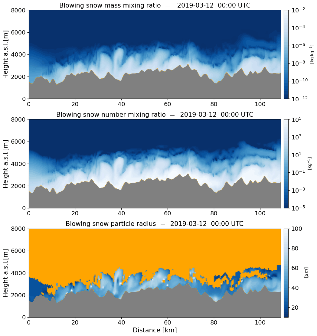
Figure 17 Blowing snow in the atmosphere on 12 March 2019 at 00:00 UTC along the transect marked by the dashed red line in Fig. 13c. (a) Blowing snow mixing ratio, (b) number mixing ratio, and (c) particle radii.

Figure 16 illustrates the horizontal variations in surface friction velocity (Fig. 16a) and blowing snow mixing ratio in the saltation layer (Fig. 16b) at 00:00 UTC on 12 March 2019. As expected in regions with complex topography, there is significant heterogeneity in surface shear stress. Saltation mixing ratio is a diagnostic quantity that is linked to the surface friction velocity and the state of the cohesion of the snowpack's surface through complex, nonlinear relationships (see Sect. 2.3). Recall that the saltation mixing ratio acts as the boundary condition for blowing snow equations for snow in suspension. High values of saltation mixing ratios are found in regions of topographic prominence such as ridges and the high-altitude region in the centre of the domain. However, there is no saltation occurrence in the lower-lying parts of the domain. This is not only due to lower wind speeds but also due to the fact that the cohesion is higher at low altitudes due to warmer air temperatures.

Saltation occurs very close to the surface, within a height of centimetres. However, snow in suspension, though many orders of magnitude lower in concentration, undergoes long-range transport, both horizontally and vertically. In classical boundary layer meteorology, transport in the horizontal and the vertical is driven mostly by advection and turbulent mixing, respectively. However, in alpine regions, the interplay between complex topography and atmospheric stability results in a wide range of complex flow types, such as orographic waves, rotors, katabatic and anabatic winds, etc. Such motions can be significant sources of vertical advection of blowing snow. These features are also active in preferential deposition of precipitating snow (Lehning et al., 2008; Gerber et al., 2018). Enhanced vertical displacement of blowing snow particles further increases their propensity for horizontal transport due to higher wind speeds aloft.

An illustration of the complexity of blowing snow clouds is shown in Fig. 17, which shows the blowing snow mass and number mixing ratios (Fig. 17a and b, respectively) along a vertical cross section located at the dashed red line shown in Fig. 13c. While blowing snow quantities are not significant from a surface mass balance perspective, they are relevant from a microphysics perspective. From this point of view, blowing snow particles can be found even 1000 m above the surface and at some locations with values of the order of 0.01 kg kg⁻¹. While it is not well known at the moment whether blowing snow particles trigger any microphysics feedback processes, for example, acting as seeders for cloud formation, CRYOWRF can be used for further research in this direction. The final subplot in Fig. 17 shows the mean particle radius, which is a diagnostic variable from the blowing snow module. There is qualitatively a trend of decreasing radii with height, even though there are significant variations from this. There are cases, for example, where even 100 µm particles are found at significant altitudes above the surface. A video that shows the dynamics of the blowing snow mixing ratios for the entire simulation period is provided as Video M2 in the Supplement.

There is an important caveat to values of blowing snow presented in this case study (apart from the lack of verification with field measurements). As described in the previous section, the snowpack was initialized using single-layer snow information from COSMO-1 analysis fields. Surface grain diameters and cohesion between the grains were arbitrarily chosen. For very short simulations, as in this case study, the initial conditions of the snowpack can play a critical role in modulating the simulation results. The ideal way of initializing the snowpack would be by first running Alpine3D (the spatially distributed version of SNOWPACK) forced by meteorological or even COSMO-1 analyses fields for the domain of interest and initializing the snowpacks within CRYOWRF from the outputs of Alpine3D. This would provide a reasonably correct state of snowpacks at the start of the simulation. Such a workflow would be followed in dedicated studies focused on the verification of CRYOWRF for alpine simulations.

5 Summary and outlook

This article describes the first version of CRYOWRF, a new modelling framework to simulate atmospheric flows and snowpack dynamics in cryospheric environments. CRYOWRF is an extension of the widely used atmospheric model, WRF, with an advanced-complexity snow model, SNOWPACK, acting as the land surface model. Additionally, CRYOWRF includes a novel blowing snow scheme, a modelling capability not available in publicly released versions of WRF. The development of CRYOWRF was guided by three main design goals. First, that the entire workflow, from compilation, pre-processing, and running the simulation to finally post-processing of simulation output, must be as close as possible to standard WRF. The second goal was to ensure that all the technical capabilities of WRF, such as hybrid (MPI+OpenMP) parallelism, multiple nesting, input/output, and start–stop–restart capabilities were maintained. The final goal was to create a coupling framework such that CRYOWRF remains agnostic to the versions of the underlying WRF and SNOWPACK models.

Apart from a model description, three case studies were presented that showcase the suitability of CRYOWRF for simulating coupled atmospheric flow and snowpack dynamics over polar ice sheets on the one hand (case study I) and snow-covered alpine topography on the other (case study II). The cases show that processes which have been inaccessible to previous mesoscale modelling efforts can be simulated using CRYOWRF. In case study Ia (Sect. 4.1), results from a year-long simulation over the entire continent of Antarctica were compared with station measurements to establish the accuracy of the model. In case study Ib, CRYOWRF was applied to simulate a complex atmospheric flow phenomenon involving the formation of a hydraulic jump and gravity wave excitation along the entrainment and vertical advection of blowing snow particles off the east Antarctica coast. This phenomenon can only be captured using resolutions of 𝒪 (1 km). None of the pre-eminent models for Antarctica research (RACMO/MAR) can simulate such phenomena due to their hydrostatic dynamical core; this is a limitation CRYOWRF does not have. The final case study (case study II; Sect. 4.3) showcases the applicability of CRYOWRF for simulations in snow-covered alpine terrain at resolutions of 𝒪 (100 m). Even though such simulations have been performed in the past with alternate modelling frameworks such as Meso-NH, standard WRF cannot perform such simulations due to the lack of a blowing snow model, which is a shortcoming that CRYOWRF remedies.

Apart from highlighting model capabilities, these case studies also serve as templates for potential users who may wish to adopt CRYOWRF for their own research. All the necessary name lists, Python helper scripts to create the snowpack initial conditions, post-processing scripts for data analysis and plotting, along with descriptions of the workflow for each of the these case studies, are provided to act as user guides. The code is, of course, made publicly available (see the data availability section for more details). As this is the first version of CRYOWRF, there are many directions to take as far as the future roadmap is concerned. One direction is to establish model accuracy through verification studies comparing model outputs with weather station and remote sensing datasets. The analyses presented in case study Ia are being expanded with intercomparison with far more extensive measurement datasets and will be presented in a forthcoming publication. Case studies Ib and II are also starting points for more detailed analyses and can shed light on hitherto underexplored aspects of impact of blowing snow on components on the atmospheric system, such as cloud dynamics and radiative effects. These set-ups need further verification.

The other direction, in a longer time frame, is to expand the applicability of CRYOWRF to other areas of the cryospheric environment not considered in this article. The two most promising areas for expansion are to test CRYOWRF for modelling sea ice–atmosphere interaction and snow–forest–atmosphere interaction. In each of these two cases, the underlying SNOWPACK model has been used in single-column, measurement-forced set-ups in previous publications (see the Introduction for references), providing guidance in setting up CRYOWRF for simulations in these cryospheric environments.

The development of CRYOWRF can be viewed from various different perspectives. On the one hand, it can purely be seen as an improvement in the capabilities of the standard WRF for cryospheric regions. If existing users of WRF who are working on topics related to cryospheric environments find CRYOWRF useful, then that in itself would make the effort required for its development worthwhile. However, the other, more general perspective is to consider CRYOWRF as model that combines a mature, advanced atmospheric model core with a mature, high-complexity snow cover model allowing the exploration of poorly understood or novel cryospheric phenomena and feedback loops. From this perspective, CRYOWRF carries with it the promise that the sum may be greater than its parts.

Appendix A: New name list settings for CRYOWRF

CRYOWRF is a superset of WRF in the sense that it adds SNOWPACK as LSM to WRF. Recall that WRF is the master model, and thus, all WRF-SNOWPACK interactions are governed by WRF and its name list. In Table A1, new name list variables for CRYOWRF are listed. All the new name list variables are in the physics section of the WRF name list. Examples of name lists can be found in the reproducibility (simulation) dataset.

Table A1 New name list variables for CRYOWRF.