AvaFrame com1DFA (v1.3): a thickness-integrated computational avalanche module – theory, numerics, and testing

Simulation tools are important to investigate and predict mobility and the destructive potential of gravitational mass flows (e.g., snow avalanches). AvaFrame – the open avalanche framework – offers well-established computational modeling approaches, tools for data handling and analysis, and ready-to-use modules for evaluation and testing. This paper presents the theoretical background, derivation, and model verification for one of AvaFrame's core modules, the thickness-integrated computational model for avalanches with flow or mixed form of movement, named com1DFA. Particular emphasis within the description of the utilized numerical particle–grid method is given to the computation of spatial gradients and the accurate implementation of driving and resisting forces. The implemented method allows us to provide a time–space criterion connecting the numerical particles, grid, and time discretization. The convergence and robustness of the numerical implementation is checked with respect to the spatiotemporal evolution of the flow variables using tests with a known analytical solution. In addition, we present a new test for verifying the accuracy of the numerical simulation in terms of runout (angle and distance). This test is derived from the total energy balance along the center-of-mass path of the avalanche. This article, particularly in combination with the code availability (open-source code repository) and detailed online documentation provides a description of an extendable framework for modeling and verification of avalanche simulation tools.

1 Introduction

Simulation tools for gravitational mass flows – with a focus on snow avalanches in this article – are in great demand for operational engineering applications and scientific model development and are gaining increasing attention in academic education. Each of these application requires different outputs. For operational engineering applications, the runout outcome for different scenarios is usually of highest interest. Scientific applications aim at better understanding the processes and will require outputs such as flow variable evolution. Existing tools for simulating snow avalanches cover a wide range of numerical implementations and vary from proprietary (e.g., Christen et al., 2010; Sampl and Zwinger, 2004; Zugliani and Rosatti, 2021; Li et al., 2021) to open-source software (e.g., Hergarten and Robl, 2015; Mergili et al., 2017; Rauter et al., 2018). The latter ones are generally more focused towards scientific and academic issues, whereas the first are more geared towards operational applications. AvaFrame – the open avalanche framework – strives to fill the gap between operations and scientific development combining over a decade of operational application (using, e.g., SamosAT; see Sampl and Zwinger, 2004; Fischer et al., 2014) with an open-source scientific development environment. Using a modular structure AvaFrame adds in-depth testing and analysis modules to the core flow modules. Further modules provide interfaces for visualization and geodata handling for all kinds of existing and emerging simulation tools. It enables us to combine, further develop, and extend the different tools to best suit the users needs.

At their core, avalanche simulation tools are based on a large variety of flow models, differing in their basic assumptions (what physical processes they include, degree of complexity), mathematical derivation, and/or their numerical implementation. These range from Eulerian methods (Christen et al., 2010; Mergili et al., 2017; Rauter and Tuković, 2018; Zugliani and Rosatti, 2021) using spatially fixed meshes to Lagrangian methods (Sampl and Zwinger, 2004) where the mass is discretized. Some methods are combinations of Eulerian and Lagrangian approaches, such as the Material Point method (Stomakhin et al., 2013). AvaFrame's com1DFA dense-flow avalanche (DFA) module is based on a flow model that is derived from the thickness integration of the conservation equations of mass and momentum. Classic shallow-water models, e.g., Saint-Venant, integrate in the direction of gravity, often called “depth” integration. Other approaches, such as Savage–Hutter models (Savage and Hutter, 1989) integrate in the slope-normal direction but also call it “depth” integrated. To be more consistent with operational terminology, we propose calling the integration in the slope-normal direction “thickness” integration. In this way, we can highlight the special case of gravitational mass flows in steep terrain.

The resulting equations are solved using a mixed particle–grid method, in which mass is tracked using particles. Pressure gradients are computed using a smooth particle hydrodynamics (SPH) method adapted to steep terrain and flow thickness is computed on the grid (Sampl and Zwinger, 2004; Monaghan, 2005; Liu and Liu, 2010; Granig et al., 2016). To avoid nonphysical behavior at starting and stopping, com1DFA applies the method proposed in Mangeney-Castelnau et al. (2003), allowing for a friction balanced starting and stopping of the flow.

Verifying and validating the methods applied in our implementation is a challenging but crucial step, as it is for all simulation tools. Verification is done by comparing the numerical model results to an analytical solution (e.g., Zugliani and Rosatti, 2021; Rauter and Tuković, 2018). Validation can be tackled in different ways, either by comparing the model results to observations (e.g., Christen et al., 2010) or by comparing them to the results of already trusted numerical models. In this article, the focus is on model verification, and the numerical model results are compared to tests with known (semi-)analytical solutions using two different approaches.

The flow variable tests (Hutter et al., 1993; Faccanoni and Mangeney, 2013) allow us to investigate the local spatiotemporal evolution of flow thickness and velocity. This enables us to verify the proper implementation of the pressure gradient and friction force computation among others. In contrast, the energy line test is based on the investigation of the total energy balance (Körner, 1980). It focuses on the accuracy of the global kinetic energy (velocity) along the path and the corresponding center-of-mass runout. Thereby, the proper implementation of stopping behavior, that is to say the proper balancing of driving and friction forces, can be assessed. It also provides a test where the runout, a quantity which is important for operational applications, is tested. We explore and explain the limitations of these two approaches.

The article is structured as follows. Section 2 summarizes the underlying flow model, including fundamental assumptions and derivations of the thickness-integrated equations, building the foundation for the gravitational mass flow simulations. In Sect. 3 the temporal and spatial discretizations of the model equations, employing a particle–grid approach, are described. The implementation in the AvaFrame computational module com1DFA is outlined in Sect. 4. Model verification tests are presented in Sect. 5, targeting the correct implementation of the mathematical model and the convergence and robustness of the numerical model code. In addition to employing test cases with a known (semi-)analytical solution, a new energy line test is introduced in Sect. 5.2.

Besides the in-depth description within this article, Oesterle et al. (2022) provide a combination of code and corresponding documentation. Users find more information according to their individual scientific, operational, or educational focus, and the reader is invited to contribute to the future development. It is important to note that this article presents the latest development state of the com1DFA module. It differs slightly from the implementation of the com1DFA module used for operational purposes, which is described in the online AvaFrame documentation. For example, differences include improvements of the SPH gradient computation method and how friction forces are taken into account.

2 Mathematical model: from 3D equations to thickness-integrated Lagrangian equations

In this section, the mathematical model and associated equations used to simulate DFA processes are presented. The derivation is based on the thickness integration of the three-dimensional Navier–Stokes equations, using a Lagrangian approach with a terrain-following coordinate system. The equations are simplified using the assumption of shallow flow on a mildly curved topography, meaning flow thickness is considerably smaller than the length and width of the avalanche, and it is considerably smaller than the topography curvature radius.

We consider snow as the material; however, the choice of material does not influence the derivation in the first place. We assume constant density ρ₀ and a flow on a surface 𝒮, subjected to the gravity force and friction on the surface 𝒮. If needed, additional processes such as entrainment or other external effects can be taken into account. These processes are included in the following derivations but will not be considered for model verification (Sect. 5), as test cases with an analytical solution are only available for simplified conditions where entrainment or any additional forces are discarded. The mass conservation equation applied to a Lagrangian volume of material V(t) reads:

$$\begin{array}{}\text{(1)}& {\displaystyle \frac{\mathrm{d}}{\mathrm{d}t}}\underset{m\left(t\right)}{\underbrace{\underset{V\left(t\right)}{\int }{\mathit{\rho }}_{\mathrm{0}}\mathrm{d}V}}={\mathit{\rho }}_{\mathrm{0}}{\displaystyle \frac{\mathrm{d}V\left(t\right)}{\mathrm{d}t}}=\underset{\partial V\left(t\right)}{\oint }{q}^{\text{ent}}\mathrm{d}A,\end{array}$$

where the source term q^ent represents the snow entrainment rate (incoming mass flux). The momentum conservation equation applied to the same volume of material V(t) reads as follows:

$$\begin{array}{}\text{(2)}& {\displaystyle \frac{\mathrm{d}}{\mathrm{d}t}}\underset{V\left(t\right)}{\int }{\mathit{\rho }}_{\mathrm{0}}\mathit{u}\mathrm{d}V=\underset{\text{surface forces}}{\underbrace{\underset{\partial V\left(t\right)}{\oint }\mathit{\sigma }\cdot \mathit{n}\mathrm{d}A}}+\underset{\text{body force}}{\underbrace{\underset{V\left(t\right)}{\int }{\mathit{\rho }}_{\mathrm{0}}\mathit{g}\mathrm{d}V}}+{\mathbf{F}}^{\text{ext}},\end{array}$$

where u is the fluid velocity and g the gravity acceleration. $\mathit{\sigma }=-p\text{𝟙}+\mathbf{T}$ represents the stress tensor, where 𝟙 is the identity tensor, p the pressure, and T the deviatoric part of the stress tensor. n is the normal vector on ∂V(t). F^ext represents additional forces due to snow entrainment (force needed to break and compact the entrained snow) or due to added resistance (trees, obstacles, etc.). F^ext is assumed to be surface parallel. Problem-specific assumptions are needed to solve the mass and momentum conservation equations (closure equation on the stress tensor in Sect. 2.2). These constitutive equations are introduced in the following sections alongside a local coordinate system and boundary conditions.

2.1 Natural coordinate system (NCS) and thickness-integrated quantities

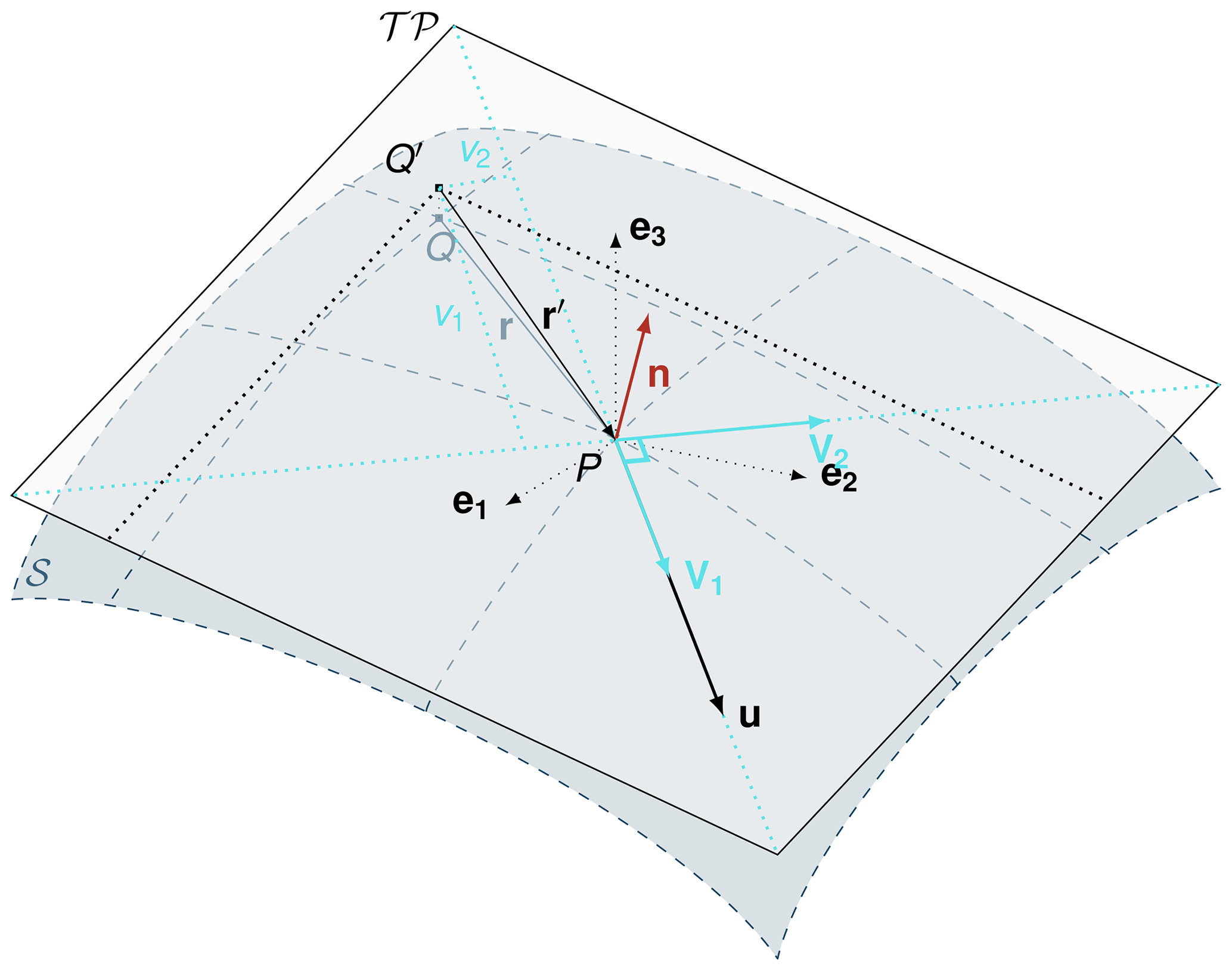
In order to solve the previously described equations, a local coordinate system is introduced. The avalanche flows on a surface 𝒮, a 2D manifold embedded in the 3D Euclidian space. Different approaches exist to define a coordinate system on this curved surface. Some define a tangent space in every point on 𝒮 based on the coordinate lines, which leads to an orthogonal but not orthonormal coordinate system for a curved surface 𝒮 (e.g., Luca et al., 2016). Instead of this and because of the Lagrangian approach used here, we define a local coordinate system in the tangent plane to 𝒮 at any point using the velocity direction and the normal to the surface 𝒮 at this position. This results in a time-dependent orthonormal coordinate system that is advected along with the flow, referred to as the natural coordinate system (NCS).

A control volume V(t) is assumed to be a small truncated pyramid shape extending from the bottom surface 𝒮_b (lying on the topography 𝒮) up to the free surface in the surface-normal direction N^b as illustrated in Fig. 1. With the assumption of moderately curved surfaces, this is close to being a prism shape since the normals of the lateral surfaces are almost parallel to the bottom. Note that the bottom surface 𝒮_b of area A^b has no predefined shape. The octagonal shape used in Fig. 1 is just one possible option.

The normal vector N^b to the bottom surface is pointing upwards, whereas ${\mathit{n}}^{\mathrm{b}}=-{\mathit{N}}^{\mathrm{b}}$ is the bottom normal vector to the Lagrangian control volume (pointing out of the volume).

$$\begin{array}{}\text{(3)}& V\left(t\right)=\underset{V\left(t\right)}{\int }\mathrm{d}V=\underset{{\mathcal{S}}_{\mathrm{b}}}{\int }\left(\underset{\mathrm{b}}{\overset{s}{\int }}\det \left(\mathbf{J}\right)\mathrm{d}{x}_{\mathrm{3}}\right)\mathrm{d}A,\end{array}$$

where J is the transformation matrix from the Cartesian coordinate system to the NCS. The NCS is an orthonormal coordinate system $({\mathit{v}}_{\mathrm{1}},{\mathit{v}}_{\mathrm{2}},{\mathit{v}}_{\mathrm{3}})$ aligned with the bottom surface. ${\mathit{v}}_{\mathrm{3}}={\mathit{N}}^{\mathrm{b}}=-{\mathit{n}}^{\mathrm{b}}$ is the normal vector to the bottom surface pointing upwards. v₁ is pointing in the direction of the thickness-integrated fluid velocity $\stackrel{\mathrm{‾}}{\mathit{u}}$ (introduced below).

$$\begin{array}{}\text{(4)}& {\mathit{v}}_{\mathrm{1}}={\displaystyle \frac{\stackrel{\mathrm{‾}}{\mathit{u}}}{\left|\left|\stackrel{\mathrm{‾}}{\mathit{u}}\right|\right|}},{\mathit{v}}_{\mathrm{2}}={\displaystyle \frac{{\mathit{v}}_{\mathrm{3}}\wedge {\mathit{v}}_{\mathrm{1}}}{\left|\left|{\mathit{v}}_{\mathrm{3}}\wedge {\mathit{v}}_{\mathrm{1}}\right|\right|}},{\mathit{v}}_{\mathrm{3}}={\mathit{N}}^{\mathrm{b}}.\end{array}$$

In the case of shallow flow on weakly curved surfaces, $\det \left(\mathbf{J}\right)=(\mathrm{1}-{\mathit{\kappa }}_{\mathrm{1}}{x}_{\mathrm{3}})(\mathrm{1}-{\mathit{\kappa }}_{\mathrm{2}}{x}_{\mathrm{3}})\approx \mathrm{1}$. κ_{1,2} represents the surface curvature in v_{1,2} directions, while x₃ is the elevation from the bottom surface in the direction N^b. This approximation is valid if the curvature radius is much larger than the flow thickness h. In this case, the control volume reads as follows:

$$\begin{array}{}\text{(5)}& V\left(t\right)\approx \underset{{\mathcal{S}}_{\mathrm{b}}}{\int }\underset{h\left(t\right)}{\underbrace{\underset{\mathrm{b}}{\overset{s}{\int }}\mathrm{d}{x}_{\mathrm{3}}}}\mathrm{d}A.\end{array}$$

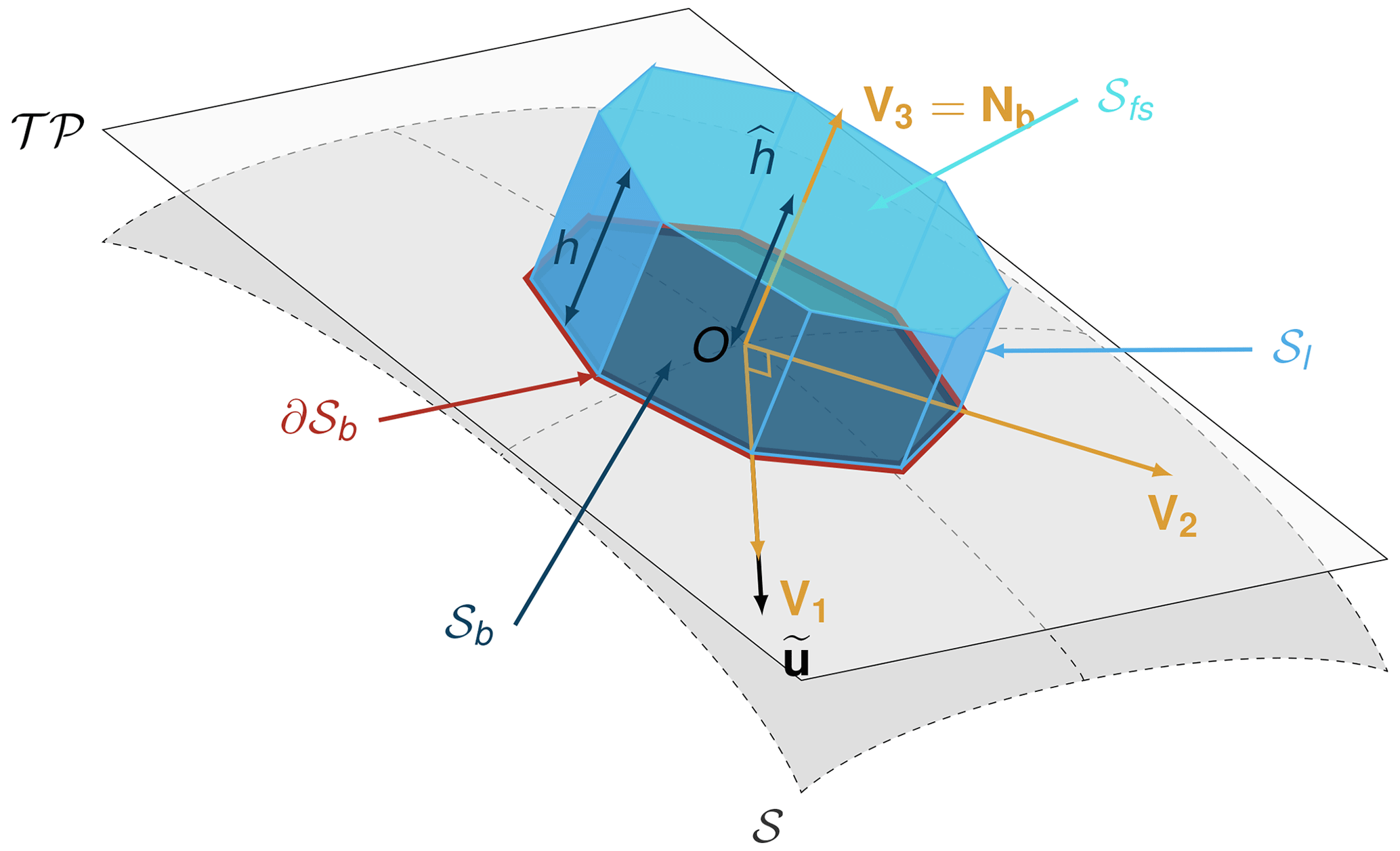
Figure 1 Example of a small Lagrangian volume considered in the equations and corresponding notations. The gray surface (denoted 𝒮) represents the bottom surface (topography), and 𝒯𝒫 represents the tangent plane to the surface at the point O. The normal vector to 𝒮 and 𝒯𝒫 in O is v₃=N^b. The control volume, represented in blue, has a basal surface 𝒮_b lying in 𝒯𝒫, a lateral surface 𝒮_l aligned with N^b, and a free surface 𝒮_fs.

The following volume (indicated by the superscript $\stackrel{\mathrm{̃}}{\square }$), area (indicated by the superscript $\widehat{\square }$), and thickness (indicated by the superscript $\stackrel{\mathrm{‾}}{\square }$) averaged quantities are introduced (where f is a scalar or vector function on Ω⊂ℛ³):

$$\begin{array}{}\text{(6)}& \begin{array}{rl}\begin{array}{ll}\stackrel{\mathrm{̃}}{f}& =\frac{\mathrm{1}}{V\left(t\right)}\underset{V\left(t\right)}{\int }f\mathrm{d}V\\ \widehat{f}& =\frac{\mathrm{1}}{A^{\mathrm{b}}\left(t\right)}\underset{{\mathcal{S}}_{\mathrm{b}}}{\int }f\mathrm{d}A\\ \stackrel{\mathrm{‾}}{f}& =\frac{\mathrm{1}}{h\left(t\right)}\underset{\mathrm{0}}{\overset{h\left(t\right)}{\int }}f\mathrm{d}{x}_{\mathrm{3}}\end{array}& \text{and}\stackrel{\mathrm{̃}}{f}\left(x_{\mathrm{3}}\right)={\displaystyle \frac{\mathrm{1}}{A^{\mathrm{b}}(\widehat{h}-x_{\mathrm{3}})}}\underset{{\mathcal{S}}_{\mathrm{b}}}{\int }\left(\underset{x_{\mathrm{3}}}{\overset{h\left(t\right)}{\int }}f\det \left(\mathbf{J}\right)\mathrm{d}{x}_{\mathrm{3}}\right)\mathrm{d}A\\ & \approx {\displaystyle \frac{\mathrm{1}}{A^{\mathrm{b}}(\widehat{h}-x_{\mathrm{3}})}}\underset{{\mathcal{S}}_{\mathrm{b}}}{\int }\left(\underset{x_{\mathrm{3}}}{\overset{h\left(t\right)}{\int }}f\mathrm{d}{x}_{\mathrm{3}}\right)\mathrm{d}A\\ & \stackrel{\mathrm{‾}}{f}\left(x_{\mathrm{3}}\right)={\displaystyle \frac{\mathrm{1}}{(h-x_{\mathrm{3}})}}\underset{x_{\mathrm{3}}}{\overset{h\left(t\right)}{\int }}f\mathrm{d}{x}_{\mathrm{3}}.\end{array}\end{array}$$

Note that $\stackrel{\mathrm{̃}}{f}\left(\mathrm{0}\right)=\stackrel{\mathrm{̃}}{f}$ and $\stackrel{\mathrm{‾}}{f}\left(\mathrm{0}\right)=\stackrel{\mathrm{‾}}{f}$. When the control volume goes to 0, i.e., basal area goes to a point, $\stackrel{\mathrm{̃}}{f}\stackrel{A^{\mathrm{b}}\to \mathrm{0}}{⟶}\stackrel{\mathrm{‾}}{f}$ and $\widehat{f}\stackrel{A^{\mathrm{b}}\to \mathrm{0}}{⟶}f$. Also, note that we assume integration on a tangent plane being equivalent to integration on a small surface in the manifold defined by the terrain (or 3D space in which the terrain is embedded). This is justified by the relative smallness of the basal particle surface compared to the curvature.

The NCS has some interesting properties that will be useful for projecting and solving the equations. Because of the orthogonality of this NCS, we have ${\mathit{v}}_i\cdot {\mathit{v}}_j={\mathit{\delta }}_{ij},\mathit{\{}i,j\mathit{\}}\in \mathit{\{}\mathrm{1},\mathrm{2},\mathrm{3}{\mathit{\}}}^{\mathrm{2}}$, which gives after time derivation:

$$\begin{array}{}\text{(7)}& {\displaystyle \frac{\mathrm{d}({\mathit{v}}_i\cdot {\mathit{v}}_j)}{\mathrm{d}t}}={\mathit{v}}_i\cdot {\displaystyle \frac{\mathrm{d}{\mathit{v}}_j}{\mathrm{d}t}}+{\displaystyle \frac{\mathrm{d}{\mathit{v}}_i}{\mathrm{d}t}}\cdot {\mathit{v}}_j=\mathrm{0},\end{array}$$

meaning that

$$\begin{array}{}\text{(8)}& \left\{\begin{array}{ll}\frac{\mathrm{d}{\mathit{v}}_i}{\mathrm{d}t}\cdot {\mathit{v}}_i& =\mathrm{0}⟹\frac{\mathrm{d}{\mathit{v}}_i}{\mathrm{d}t}⟂{\mathit{v}}_i\\ \frac{\mathrm{d}{\mathit{v}}_i}{\mathrm{d}t}\cdot {\mathit{v}}_j& =-{\mathit{v}}_i\cdot \frac{\mathrm{d}{\mathit{v}}_j}{\mathrm{d}t},i\ne j.\end{array}\right.\end{array}$$

It is possible to express $\frac{\mathrm{d}{\mathit{v}}_{\mathrm{1}}}{\mathrm{d}t}$ in terms of $({\mathit{v}}_{\mathrm{1}},{\mathit{v}}_{\mathrm{2}},{\mathit{v}}_{\mathrm{3}})$ and using orthogonality of $\frac{\mathrm{d}{\mathit{v}}_i}{\mathrm{d}t}$ and v_i:

$$\begin{array}{}\text{(9)}& {\displaystyle \frac{\mathrm{d}{\mathit{v}}_{\mathrm{1}}}{\mathrm{d}t}}={\mathit{\alpha }}_i{\mathit{v}}_i=\textcolor{red}{}+{\mathit{\alpha }}_{\mathrm{2}}{\mathit{v}}_{\mathrm{2}}+{\mathit{\alpha }}_{\mathrm{3}}{\mathit{v}}_{\mathrm{3}},{\mathit{\alpha }}_i={\displaystyle \frac{\mathrm{d}{\mathit{v}}_{\mathrm{1}}}{\mathrm{d}t}}\cdot {\mathit{v}}_i.\end{array}$$

The derivative of the thickness-integrated velocity decomposes to

$$\begin{array}{}\text{(10)}& \begin{array}{rl}{\displaystyle \frac{\mathrm{d}\stackrel{\mathrm{‾}}{\mathit{u}}}{\mathrm{d}t}}& ={\displaystyle \frac{\mathrm{d}\left({\stackrel{\mathrm{‾}}{u}}_{\mathrm{1}}{\mathit{v}}_{\mathrm{1}}\right)}{\mathrm{d}t}}={\stackrel{\mathrm{‾}}{u}}_{\mathrm{1}}{\displaystyle \frac{\mathrm{d}{\mathit{v}}_{\mathrm{1}}}{\mathrm{d}t}}+{\displaystyle \frac{\mathrm{d}{\stackrel{\mathrm{‾}}{u}}_{\mathrm{1}}}{\mathrm{d}t}}{\mathit{v}}_{\mathrm{1}}={\stackrel{\mathrm{‾}}{u}}_{\mathrm{1}}({\mathit{\alpha }}_{\mathrm{2}}{\mathit{v}}_{\mathrm{2}}+{\mathit{\alpha }}_{\mathrm{3}}{\mathit{v}}_{\mathrm{3}})\\ & +{\displaystyle \frac{\mathrm{d}{\stackrel{\mathrm{‾}}{u}}_{\mathrm{1}}}{\mathrm{d}t}}{\mathit{v}}_{\mathrm{1}}.\end{array}\end{array}$$

2.2 Boundary conditions

To complete the conservation Eqs. (1) and (2) the following boundary conditions at the bottom (𝒮_b) and free (𝒮_fs) surfaces are introduced. σ_s and σ_b represent the restriction of σ to the free surface 𝒮_fs and bottom surface 𝒮_b, respectively:

• traction-free top surface –

  $$\begin{array}{}\text{(11)}& {\mathit{\sigma }}_{\mathbf{s}}\cdot {\mathit{n}}_{\mathrm{s}}=\mathbf{0}\text{on}{\mathcal{S}}_{\mathrm{fs}};\end{array}$$

• impenetrable bottom surface without detachment –

  $$\begin{array}{}\text{(12)}& {\mathit{u}}^{\mathrm{b}}\cdot {\mathit{n}}^{\mathrm{b}}=\mathbf{0}\text{on}{\mathcal{S}}_b;\end{array}$$

• bottom friction law –

  $$\begin{array}{}\text{(13)}& \begin{array}{rl}{\mathit{\tau }}^{\mathrm{b}}& ={\mathit{\sigma }}^{\mathrm{b}}\cdot {\mathit{n}}^{\mathrm{b}}-\left(\right({\mathit{\sigma }}^{\mathrm{b}}\cdot {\mathit{n}}^{\mathrm{b}})\cdot {\mathit{n}}^{\mathrm{b}}){\mathit{n}}^{\mathrm{b}}\\ & =f({\mathit{\sigma }}^{\mathrm{b}},\stackrel{\mathrm{‾}}{\mathit{u}},h,{\mathit{\rho }}_{\mathrm{0}},t,\mathit{x})\\ & =-f({\mathit{\sigma }}^{\mathrm{b}},\stackrel{\mathrm{‾}}{\mathit{u}},h,{\mathit{\rho }}_{\mathrm{0}},t,\mathit{x}){\mathit{v}}_{\mathrm{1}}\text{on }{\mathcal{S}}_b.\end{array}\end{array}$$

2.3 Constitutive relation: friction force

To close the momentum equation, a constitutive equation describing the basal shear stress tensor τ^b as a function of the avalanche flow state is required:

$$\begin{array}{}\text{(14)}& {\mathit{\tau }}^{\mathrm{b}}=f{\mathit{\sigma }}^{\mathrm{b}},\stackrel{\mathrm{‾}}{\mathit{u}},h,{\mathit{\rho }}_{\mathrm{0}},t,\mathit{x}).\end{array}$$

The model verification tests (Sect. 5) are carried out with a Mohr–Coulomb friction model, which describes the friction interaction between two solids. The bottom shear stress reads as follows:

$$\begin{array}{}\text{(15)}& {\mathit{\tau }}^{\mathrm{b}}=-\tan \mathit{\delta }{\mathit{\sigma }}^{\mathrm{b}}\cdot {\mathit{n}}^{\mathrm{b}}{\displaystyle \frac{\stackrel{\mathrm{‾}}{\mathit{u}}}{\left|\left|\stackrel{\mathrm{‾}}{\mathit{u}}\right|\right|}},\end{array}$$

where δ is the friction angle and μ=tan δ is the friction coefficient. The bottom shear stress linearly increases with the normal stress component p^b.

With Mohr–Coulomb friction an avalanche starts to flow if the slope inclination exceeds the friction angle δ. In the case of an infinite slope of constant inclination, the avalanche velocity would increase indefinitely. However, because of its relative simplicity, the Mohr–Coulomb friction model is convenient for deriving analytical solutions and testing numerical implementations. For a more detailed discussion of friction laws and their applicability, we refer to Salm and Gubler (1985); Gubler (1987); Gauer (2014).

Different friction models accounting for the influence of flow velocity, flow thickness, etc., have been proposed. Three friction models are available in the com1DFA module. First, a Coulomb one, which is used in this paper, second a Voellmy friction model (Voellmy, 1955), and third the samosAT friction model, which is the one used for hazard mapping by Austrian federal agencies (Sampl, 2007).

2.4 Expression of surface forces in the NCS

Taking advantage of the NCS and using the boundary conditions, it is possible to split the surface forces into bottom, lateral, and free surface forces and perform further simplifications:

$$\begin{array}{}\text{(16)}& \textcolor{red}{}\end{array}$$

Using the notations introduced in Sect. 2.1 and the decomposition of the stress tensor, the bottom force can be expressed as a surface-normal component and a surface-tangential one:

$$\begin{array}{}\text{(17)}& \begin{array}{rl}\underset{{\mathcal{S}}_{\mathrm{b}}}{\int }{\mathit{\sigma }}^{\mathrm{b}}\cdot {\mathit{n}}^{\mathrm{b}}\mathrm{d}A& =\underset{{\mathcal{S}}_{\mathrm{b}}}{\int }(-p^{\mathrm{b}}\text{𝟙}+\mathbf{T})\cdot {\mathit{n}}^{\mathrm{b}}\mathrm{d}A=-\underset{{\mathcal{S}}_{\mathrm{b}}}{\int }{p}^{\mathrm{b}}{\mathit{n}}^{\mathrm{b}}\mathrm{d}A\\ & +\underset{{\mathcal{S}}_{\mathrm{b}}}{\int }\mathbf{T}\cdot {\mathit{n}}^{\mathrm{b}}\mathrm{d}A=-\underset{{\mathcal{S}}_{\mathrm{b}}}{\int }{p}^{\mathrm{b}}{\mathit{n}}^{\mathrm{b}}\mathrm{d}A\\ & +\underset{{\mathcal{S}}_{\mathrm{b}}}{\int }{\mathit{\tau }}^{\mathrm{b}}\mathrm{d}A=-A^{\mathrm{b}}\widehat{p^{\mathrm{b}}{\mathit{n}}^{\mathrm{b}}}+A^{\mathrm{b}}\widehat{{\mathit{\tau }}^{\mathrm{b}}},\end{array}\end{array}$$

where τ^b is the basal friction term (introduced in Sect. 2.2). Applying Green's theorem, the lateral force reads as follows:

$$\begin{array}{}\text{(18)}& \begin{array}{rl}\underset{\partial {\mathcal{S}}_{\mathrm{b}}}{\oint }\left(\underset{\mathrm{0}}{\overset{h}{\int }}\mathit{\sigma }\cdot \mathit{n}\mathrm{d}{x}_{\mathrm{3}}\right)\mathrm{d}l& =\underset{\partial {\mathcal{S}}_{\mathrm{b}}}{\oint }\left(\underset{\mathrm{0}}{\overset{h}{\int }}(-p\text{𝟙}+\mathbf{T})\mathrm{d}{x}_{\mathrm{3}}\right)\cdot \mathit{n}\mathrm{d}l\\ & =-\underset{\partial {\mathcal{S}}_{\mathrm{b}}}{\oint }\left(\underset{\mathrm{0}}{\overset{h}{\int }}p\mathrm{d}{x}_{\mathrm{3}}\right)\cdot \mathit{n}\mathrm{d}l\\ & +\underset{\partial {\mathcal{S}}_{\mathrm{b}}}{\oint }\left(\underset{\mathrm{0}}{\overset{h}{\int }}\mathbf{T}\mathrm{d}{x}_{\mathrm{3}}\right)\cdot \mathit{n}\mathrm{d}l\\ & =-\underset{\partial {\mathcal{S}}_{\mathrm{b}}}{\oint }h\stackrel{\mathrm{‾}}{p}\mathit{n}\mathrm{d}l+\underset{\partial {\mathcal{S}}_{\mathrm{b}}}{\oint }h\stackrel{\mathrm{‾}}{\mathbf{T}}\cdot \mathit{n}\mathrm{d}l\\ & =-\underset{{\mathcal{S}}_{\mathrm{b}}}{\int }\mathbf{\nabla }\left(h\stackrel{\mathrm{‾}}{p}\right)\mathrm{d}A+\underset{{\mathcal{S}}_{\mathrm{b}}}{\int }\mathbf{\nabla }\cdot \left(h\stackrel{\mathrm{‾}}{\mathbf{T}}\right)\mathrm{d}A\\ & =-A^{\mathrm{b}}\widehat{\mathbf{\nabla }\left(h\stackrel{\mathrm{‾}}{p}\right)}+A^{\mathrm{b}}\widehat{\mathbf{\nabla }\cdot \left(h\stackrel{\mathrm{‾}}{\mathbf{T}}\right)}.\end{array}\end{array}$$

Equations (17) and (18) represent the thickness-integrated form of the surface forces and can now be used to write the thickness integrated momentum equation.

2.5 Thickness-integrated momentum equation

Using the definitions of average values given in Sect. 2.1 and the decomposition of the surface forces given by Eqs. (17) and (18), the momentum equation reads as follows:

$$\begin{array}{}\text{(19)}& \begin{array}{rl}{\mathit{\rho }}_{\mathrm{0}}{\displaystyle \frac{\mathrm{d}\left(V\right(t\left)\stackrel{\mathrm{̃}}{\mathit{u}}\right)}{\mathrm{d}t}}& ={\mathit{\rho }}_{\mathrm{0}}V{\displaystyle \frac{\mathrm{d}\stackrel{\mathrm{̃}}{\mathit{u}}}{\mathrm{d}t}}+{\mathit{\rho }}_{\mathrm{0}}\stackrel{\mathrm{̃}}{\mathit{u}}{\displaystyle \frac{\mathrm{d}V}{\mathrm{d}t}}=\underset{\partial V\left(t\right)}{\oint }\mathit{\sigma }\cdot \mathit{n}\mathrm{d}A\\ & +{\mathit{\rho }}_{\mathrm{0}}V\mathit{g}+{\mathbf{F}}^{\text{ext}},\end{array}\end{array}$$

which leads to

$$\begin{array}{}\text{(20)}& \begin{array}{rl}{\mathit{\rho }}_{\mathrm{0}}V{\displaystyle \frac{\mathrm{d}\stackrel{\mathrm{̃}}{\mathit{u}}}{\mathrm{d}t}}& =\underset{\begin{array}{c}\text{bottom}\\ \text{ normal force }\end{array}}{\underbrace{-A^{\mathrm{b}}\widehat{p{\mathit{n}}^{\mathrm{b}}}}}\underset{\begin{array}{c}\text{bottom}\\ \text{ shear force }\end{array}}{\underbrace{+A^{\mathrm{b}}\widehat{{\mathit{\tau }}^{\mathrm{b}}}}}\underset{\begin{array}{c}\text{lateral}\\ \text{ pressure force }\end{array}}{\underbrace{-A^{\mathrm{b}}\widehat{\mathbf{\nabla }\left(h\stackrel{\mathrm{‾}}{p}\right)}}}\underset{\begin{array}{c}\text{lateral}\\ \text{ shear force }\end{array}}{\underbrace{+\textcolor{red}{}}}\\ & +{\mathit{\rho }}_{\mathrm{0}}V\mathit{g}+{\mathbf{F}}^{\text{ext}}\underset{\begin{array}{c}\text{ speed loss due }\\ \text{ to entrainment }\end{array}}{\underbrace{-\stackrel{\mathrm{̃}}{\mathit{u}}\underset{\partial V\left(t\right)}{\oint }{q}^{\text{ent}}\mathrm{d}A.}}\end{array}.\end{array}$$

The lateral shear stress term is neglected because of its relative smallness in comparison to the other terms as shown by the dimensional analysis carried out in Gray and Edwards (2014). The mass conservation reads as follows:

$$\begin{array}{}\text{(21)}& {\mathit{\rho }}_{\mathrm{0}}{\displaystyle \frac{\mathrm{d}V}{\mathrm{d}t}}=\underset{\partial V\left(t\right)}{\oint }{q}^{\text{ent}}\mathrm{d}A.\end{array}$$

Using the approximations from Sect. 2.1, the equation of motion becomes

$$\begin{array}{}\text{(22)}& \begin{array}{rl}{\mathit{\rho }}_{\mathrm{0}}V{\displaystyle \frac{\mathrm{d}\stackrel{\mathrm{‾}}{\mathit{u}}}{\mathrm{d}t}}& =-A^{\mathrm{b}}p{\mathit{n}}^{\mathrm{b}}+A^{\mathrm{b}}{\mathit{\tau }}^{\mathrm{b}}-A^{\mathrm{b}}\mathbf{\nabla }\left(h\stackrel{\mathrm{‾}}{p}\right)+{\mathit{\rho }}_{\mathrm{0}}V\mathit{g}\\ & +{\mathbf{F}}^{\text{ext}}-\stackrel{\mathrm{‾}}{\mathit{u}}\underset{\partial V\left(t\right)}{\oint }{q}^{\text{ent}}\mathrm{d}A,\end{array}\end{array}$$

where all quantities are evaluated at the center of the basal area (point O in Fig. 1). This equation is projected in the normal direction v₃=N^b to get the expression of the basal pressure p^b. The projection of this same equation on the tangential plane leads to the differential equations satisfied by $\stackrel{\mathrm{‾}}{\mathit{u}}$.

2.5.1 Pressure distribution, thickness-integrated pressure, and pressure gradient

We can project the momentum equation (Eq. 22), using the volume between x₃ and the surface h, in the normal direction (${\mathit{v}}_{\mathrm{3}}={\mathit{N}}^{\mathrm{b}}=-{\mathit{n}}^{\mathrm{b}}$). Applying the properties of the NCS (Eq. 10) the surface-normal component of Eq. (22) reads as follows:

$$\begin{array}{}\text{(23)}& \textcolor{red}{}\end{array}$$

Neglecting the normal component of the pressure gradient gives the expression for pressure. Under the condition that $\stackrel{\mathrm{‾}}{\mathit{u}}$ is independent of x₃, pressure follows a linear profile from the bottom surface to the free surface:

$$\begin{array}{}\text{(24)}& \begin{array}{rl}p\left(x_{\mathrm{3}}\right)& ={\mathit{\rho }}_{\mathrm{0}}(h-x_{\mathrm{3}})\left\{-g_{N^{\mathrm{b}}}-\stackrel{\mathrm{‾}}{\mathit{u}}\cdot {\displaystyle \frac{\mathrm{d}{\mathit{N}}^{\mathrm{b}}}{\mathrm{d}t}}\right\}\\ & \text{and}p(x_{\mathrm{3}}=\mathrm{0})=p^{\mathrm{b}}={\mathit{\rho }}_{\mathrm{0}}h\left\{-g_{N^{\mathrm{b}}}-\stackrel{\mathrm{‾}}{\mathit{u}}\cdot {\displaystyle \frac{\mathrm{d}{\mathit{N}}^{\mathrm{b}}}{\mathrm{d}t}}\right\}.\end{array}\end{array}$$

Note that the bottom pressure should always be positive. A negative pressure is nonphysical and means that the material is not in contact with the bottom surface anymore. This can happen in the case of large velocities on convex topography. If so, the material should be in a free-fall state until it gets back in contact with the topography. A description on how this is handled within the numerical implementation can be found in Sect. 4.3.

Using Eq. (24), it is possible to express the thickness-integrated pressure $\stackrel{\mathrm{‾}}{p}$:

$$\begin{array}{}\text{(25)}& \begin{array}{rl}h\stackrel{\mathrm{‾}}{p}& =\underset{\mathrm{0}}{\overset{h}{\int }}p\left(x_{\mathrm{3}}\right)\mathrm{d}{x}_{\mathrm{3}}=-{\mathit{\rho }}_{\mathrm{0}}{\displaystyle \frac{h^{\mathrm{2}}}{\mathrm{2}}}\left(g_{{\mathit{N}}^{\mathrm{b}}}+\stackrel{\mathrm{‾}}{\mathit{u}}\cdot {\displaystyle \frac{\mathrm{d}{\mathit{N}}^{\mathrm{b}}}{\mathrm{d}t}}\right)\\ & =-{\mathit{\rho }}_{\mathrm{0}}{\displaystyle \frac{h^{\mathrm{2}}}{\mathrm{2}}}{g}^{\text{eff}},\end{array}\end{array}$$

where g^eff is the effective normal acceleration acting on the volume, including the normal component of gravity and a curvature component. Because of the utilized Lagrangian approach, the curvature terms are expressed as the temporal derivative of the normal vector $\frac{\mathrm{d}{\mathit{N}}^{\mathrm{b}}}{\mathrm{d}t}$, effectively computing the curvature along the particle trajectories. The resulting curvatures are equivalent to the ones obtained through Eulerian approaches (Fischer et al., 2012) but does not require the computation of the related κ_{1,2}.

The expression of the thickness-integrated pressure is used to derive the pressure gradient $\mathbf{\nabla }\left(h\stackrel{\mathrm{‾}}{p}\right)$. Assuming g^eff to be locally constant (i.e., effectively neglecting curvature; otherwise g^eff would remain inside the gradient operator) leads to

$$\begin{array}{}\text{(26)}& \mathbf{\nabla }\left(h\stackrel{\mathrm{‾}}{p}\right)=-{\mathit{\rho }}_{\mathrm{0}}{g}^{\text{eff}}h\mathbf{\nabla }h.\end{array}$$

2.5.2 Tangential momentum equation

Using the derived expression of the thickness-integrated pressure (Eq. 26), we project the momentum balance (Eq. 22) in the tangent plane, which leads to the following equation:

$$\begin{array}{}\text{(27)}& \begin{array}{rl}{\mathit{\rho }}_{\mathrm{0}}V\left({\displaystyle \frac{\mathrm{d}\stackrel{\mathrm{‾}}{\mathit{u}}}{\mathrm{d}t}}-\left({\displaystyle \frac{\mathrm{d}\stackrel{\mathrm{‾}}{\mathit{u}}}{\mathrm{d}t}}\cdot {\mathit{v}}_{\mathrm{3}}\right){\mathit{v}}_{\mathrm{3}}\right)& =A^{\mathrm{b}}{\mathit{\tau }}^{\mathrm{b}}-{\mathit{\rho }}_{\mathrm{0}}{g}^{\text{eff}}h{A}^{\mathrm{b}}{\mathbf{\nabla }}_{s}h\\ & +{\mathit{\rho }}_{\mathrm{0}}V{\mathit{g}}_{\mathrm{s}}+{\mathbf{F}}^{\text{ext}}\\ & -\stackrel{\mathrm{‾}}{\mathit{u}}\underset{\partial V\left(t\right)}{\oint }{q}^{\text{ent}}\mathrm{d}A,\end{array}\end{array}$$

where ${\mathbf{\nabla }}_s=\mathbf{\nabla }-(\mathbf{\nabla }\cdot {\mathit{N}}^{\mathrm{b}}){\mathit{N}}^{\mathrm{b}}$ and ${\mathit{g}}_{\mathrm{s}}=\mathit{g}-(\mathit{g}\cdot {\mathit{N}}^{\mathrm{b}}){\mathit{N}}^{\mathrm{b}}$ are the tangential component of the gradient operator and of the gravity acceleration, respectively.

After replacing the velocity derivative component in the normal direction with the expression developed in Eq. (23), Eq. (27) reads as follows:

$$\begin{array}{}\text{(28)}& \begin{array}{rl}{\mathit{\rho }}_{\mathrm{0}}V{\displaystyle \frac{\mathrm{d}\stackrel{\mathrm{‾}}{\mathit{u}}}{\mathrm{d}t}}& =A^{\mathrm{b}}{\mathit{\tau }}^{\mathrm{b}}-{\mathit{\rho }}_{\mathrm{0}}{g}^{\text{eff}}h{A}^{\mathrm{b}}{\mathbf{\nabla }}_{s}h+{\mathit{\rho }}_{\mathrm{0}}V{\mathit{g}}_{\mathrm{s}}+{\mathbf{F}}^{\text{ext}}\\ & -\stackrel{\mathrm{‾}}{\mathit{u}}\underset{\partial V\left(t\right)}{\oint }{q}^{\text{ent}}\mathrm{d}A-{\mathit{\rho }}_{\mathrm{0}}V\underset{\text{curvature acceleration}}{\underbrace{\left(\stackrel{\mathrm{‾}}{\mathit{u}}\cdot {\displaystyle \frac{\mathrm{d}{\mathit{v}}_{\mathrm{3}}}{\mathrm{d}t}}\right){\mathit{v}}_{\mathrm{3}}.}}\end{array},\end{array}$$

The curvature acceleration is in the normal direction to the tangent plane in order to keep the flow on the surface.

3 Numerical method: particle–grid approach

In the previous section, the equation of motion was derived using a Lagrangian approach. In order to solve this set of equations numerically, we employ a mix of particle and grid approaches. We discretize the material into numerical particles and solve the equation of motion, with the total avalanche mass being the sum of the mass associated with each particle. The grid is used to compute several parameters that are required for the computations, e.g., surface-normal vectors and flow thickness. Combining both approaches allows us to best exploit the advantages of each. The particle approach is used to track the mass, compute the curvature terms and the gradient of the flow thickness, and update the particle positions. The grid is used to handle the topography information and compute the flow thickness and artificial viscosity. We found this to help with numerical stability, and it is more efficient as it decreases the required number of particles. A theoretical convergence criterion is described in the last section.

3.1 Interpolation between particle and grid values

Topography information is usually provided in a raster format which corresponds to a regular rectilinear mesh on the global horizontal x–y plane, henceforth referred to as grid. In order to get information on the surface elevation and normal vectors, the topography information needs to be interpolated at the particle locations, and this needs to be repeated at each time step since the particles are moving. Similarly, the particle properties such as mass or momentum, which translate into flow thickness and velocity, also need to be interpolated onto the grid. Grid velocity is required to compute the artificial viscosity term, ensuring numerical stability; see Sect. 4.2. Grid flow thickness is used to compute the particle flow thickness, which is required for computing the frictional forces. The mesh being regular and rectilinear, we use bilinear interpolation for simplicity and efficiency. This also ensures the conservation of mass or momentum when interpolating from the particles to the grid and back. The properties of the grid and the interpolation method are detailed in the AvaFrame documentation (https://docs.avaframe.org/en/latest/DFAnumerics.html#interpolation, last access: 5 October 2023).

3.2 The particle momentum equation

Discretizing the material into particles (particle quantities are denoted by the subscript k; e.g., m_k=ρ₀V_k is the mass of particle k) leads to the following continuity equation:

$$\begin{array}{}\text{(29)}& {\displaystyle \frac{\mathrm{d}}{\mathrm{d}t}}{m}_k=A_k^{\text{ent}}{q}^{\text{ent}},\end{array}$$

where $A_k^{\text{ent}}$ is the interface area between the particle and the entrainable material while $q_k^{\text{ent}}$ represents the flux of entrained mass.

By assuming that the Lagrangian control volume V can be represented by a particle, we can derive the particle momentum equation in the normal direction and in the tangent plane:

$$\begin{array}{}\text{(30)}& \left\{\begin{array}{l}{p}_k^{\mathrm{b}}={\mathit{\rho }}_{\mathrm{0}}{h}_k{g}_k^{\text{eff}}\\ m_k\frac{\mathrm{d}{\stackrel{\mathrm{‾}}{\mathit{u}}}_k}{\mathrm{d}t}=A_k^{\mathrm{b}}{\mathit{\tau }}^{\mathrm{b}}-m_k{g}_k^{\text{eff}}{\mathbf{\nabla }}_{s}h+m_k{\mathit{g}}_{\mathrm{s}}+{\mathbf{F}}_k^{\text{ext}}\\ -{\stackrel{\mathrm{‾}}{\mathit{u}}}_k{A}_k^{\text{ent}}{q}_k^{\text{ent}}-m_k\left({\stackrel{\mathrm{‾}}{\mathit{u}}}_k\cdot \frac{\mathrm{d}{\mathit{v}}_{\mathrm{3},k}}{\mathrm{d}t}\right){\mathit{v}}_{\mathrm{3},k}.\end{array}\right.\end{array}$$

In this equation, flow thickness gradient, basal friction, and curvature acceleration terms need to be further developed and discretized.

3.3 Flow thickness and its gradient

3.3.1 Flow thickness gradient computation using SPH

To assess the flow thickness gradient, we employ an SPH method (smoothed particles hydrodynamics method (Liu and Liu, 2010)), where the gradient is directly derived from the particles and does not require any mesh. In contrast, a mesh method or an MPM (material point method) would directly use a mesh formulation to approximate the gradient or interpolate the particle properties on an underlying mesh and then approximate the gradient of the flow thickness using a mesh formulation. There are two main advantages of using SPH. First is the computational efficiency, since only the particles of interest are computed without needing to compute the area of the whole terrain (as with Eulerian methods). Second, mass transfer is not required because it is handled by the particles directly, making the implementation easier (Granig et al., 2016).

In theory, an SPH method does not require any mesh to compute the gradient. However, applying this method requires finding neighbor particles. This process can be sped up with the help of an underlying grid; different neighbor search methods are presented in Ihmsen et al. (2014), and a “uniform grid method” is used in this paper.

The SPH method is used to express a quantity (the flow thickness in our case) and its gradient at any particle location as a weighted sum of its neighbors' properties. The principle of the method is described well in Liu and Liu (2010), and the basic formula reads as follows:

$$\begin{array}{}\text{(31)}& \begin{array}{rl}f\left(x\right)\simeq \langle f\left(x\right)\rangle & =\sum _l{f}_l{A}_{l}W(x,x_l)\\ \mathbf{\nabla }f\left(x\right)\simeq \langle \mathbf{\nabla }f\left(x\right)\rangle & =-\sum _l{f}_l{A}_l\mathbf{\nabla }W(x,x_l),\end{array}\end{array}$$

where W represents the SPH-kernel function (we employ the spiky kernel; see Eq. B2) and the subscript l enumerates the neighboring particles. This kernel function is designed to satisfy the unity condition, be an approximation of the Dirac function and have a compact support domain (Liu and Liu, 2010).

This method is usually either used in a 3D space, in which particles move freely and where the weighting factor for the summation is the volume of the particle, or on a 2D horizontal plane, where the weighting factor for the summation is the area of the particle and the gradient is 2D. Here we want to compute the gradient of the flow thickness on a 2D surface (the topography) embedded in 3D space. The method used is analogous to the SPH gradient computation on the 2D horizontal plane but the gradient is 3D and tangent to the surface (co-linear to the local tangent plane). The theoretical derivation in Appendix B2 shows that the SPH computation is equivalent to applying the 2D SPH method in the local tangent plane instead of in the horizontal plane. This leads to the following SPH expression of the flow thickness gradient:

$$\begin{array}{}\text{(32)}& \mathbf{\nabla }{h}_k\simeq -\sum _l{h}_l{A}_l\mathbf{\nabla }W(x_k,x_l)=-\sum _l{\displaystyle \frac{m_l}{\mathit{\rho }}}\mathbf{\nabla }W(x_k,x_l).\end{array}$$

3.3.2 Flow thickness computation

The particle flow thickness is computed with the help of the grid. The mass of the particles is interpolated onto the grid using a bilinear interpolation method (described in Sect. 3.1). Then, dividing the mass at the grid cells by the area of the grid cells, while taking the slope of the cell into account, returns the flow thickness field on the grid. This is interpolated back to the particles, which leads to the particle flow thickness property.

We do not compute the flow thickness directly from the particle properties (mass and position) using an SPH method because it induced instabilities. Indeed, the cases where too few neighbors are found lead to very small flow thickness, which becomes an issue for flow-thickness-dependent friction laws. Note that using such an SPH method would lead to a full particle method. But since the flow thickness is only used in some cases for the friction force computation, using the previously described grid method should not affect the computation significantly.

3.4 Friction force discretization

The Coulomb friction force term in Eq. (30) for a particle reads:

$$\begin{array}{}\text{(33)}& \begin{array}{rl}{A}_k^{\mathrm{b}}{\mathit{\tau }}^{\mathrm{b}}& =-A_k^{\mathrm{b}}\tan \mathit{\delta }{p}_k^{\mathrm{b}}{\mathit{v}}_{\mathrm{1}}=-A_k^{\mathrm{b}}\tan \mathit{\delta }{\mathit{\rho }}_{\mathrm{0}}{h}_k{g}_k^{\text{eff}}{\mathit{v}}_{\mathrm{1}}\\ & =-m_k\tan \mathit{\delta }{g}_k^{\text{eff}}{\mathit{v}}_{\mathrm{1}}=-{\left|\left|{\mathbf{F}}_k^{\text{fric}}\right|\right|}_{\text{max}}{\mathit{v}}_{\mathrm{1}}.\end{array}\end{array}$$

This relation stands if the particle is moving. The starting and stopping processes satisfy a different equation and are handled differently in the numerical implementation (using the same equation would lead to nonphysical behavior). This is described in more detail in Sect. 4.5.

3.5 Time discretization

The momentum equation is solved numerically in time using an Euler time scheme. The time derivative of any quantity f is approximated by

$$\begin{array}{}\text{(34)}& {\displaystyle \frac{\mathrm{d}{f}_k}{\mathrm{d}t}}\approx {\displaystyle \frac{f_k^{n+\mathrm{1}}-f_k^n}{\mathrm{\Delta }t}},\end{array}$$

where Δt represents the time step and fⁿ=f(tⁿ), tⁿ=nΔt. For the velocity this reads as follows:

$$\begin{array}{}\text{(35)}& {\displaystyle \frac{\mathrm{d}{\stackrel{\mathrm{‾}}{\mathit{u}}}_k}{\mathrm{d}t}}\approx {\displaystyle \frac{{\stackrel{\mathrm{‾}}{\mathit{u}}}_k^{n+\mathrm{1}}-{\stackrel{\mathrm{‾}}{\mathit{u}}}_k^n}{\mathrm{\Delta }t}}.\end{array}$$

The positions of the particles are updated using a centered Euler scheme:

$$\begin{array}{}\text{(36)}& {\mathit{x}}_k^{n+\mathrm{1}}={\mathit{x}}_k^n+{\displaystyle \frac{\mathrm{\Delta }t}{\mathrm{2}m}}\left({\stackrel{\mathrm{‾}}{\mathit{u}}}_k^{n+\mathrm{1}}+{\stackrel{\mathrm{‾}}{\mathit{u}}}_k^n\right).\end{array}$$

The forces are taken into account in two subsequent steps as forces acting on the particles can be sorted into driving forces and friction forces. Friction forces act against the particle motion, only affecting the magnitude of the velocity. They can in no case become driving forces. This is why in a first step the velocity is updated with the driving forces before updating in a second step the velocity magnitude applying the friction force.

3.6 Convergence

We are looking for a criterion that relates the properties of the spatial and temporal discretization to ensure convergence of the numerical solution. Simply decreasing the time step and increasing the spatial resolution, by decreasing the grid cell size and kernel radius and increasing the number of particles, does not ensure convergence. Ben Moussa and Vila (2000) analyzed hyperbolic one- and two-dimensional, nonlinear transport equations with a particle and SPH method and showed that the kernel radius size cannot be varied independently from the time step and number of particles. Indeed, they showed that the numerical solution converges towards the solution of the equation under the following condition:

$$\begin{array}{}\text{(37)}& {\displaystyle }\left\{\begin{array}{ll}{r}_{\text{part}}& \to \mathrm{0}\\ r_{\text{kernel}}& \to \mathrm{0}\\ \frac{r_{\text{part}}^{\mathrm{2}}}{r_{\text{kernel}}^{\mathrm{3}}}& \to \mathrm{0}\end{array}\right.\text{and}\mathrm{d}t\le C{r}_{\text{kernel}},\end{array}$$

where r_part represents the “size” of a particle, r_kernel represents the SPH kernel radius, dt is the time step and C a constant. The conditions in Eq. (37) mean that both r_part (particle size) and r_kernel (SPH kernel radius) need to go to zero but also that the particle size needs to go faster to zero than the SPH kernel radius. Finally, the time step needs to go to zero at the same rate as r_kernel. The particle size can be expressed as a function of the SPH kernel radius:

$$\begin{array}{}\text{(38)}& r_{\text{part}}={\left({\displaystyle \frac{A^{\mathrm{b}}}{\mathit{\pi }}}\right)}^{\mathrm{1}/\mathrm{2}}={\left({\displaystyle \frac{A_{\text{kernel}}}{\mathit{\pi }{n}_{\text{ppk}}}}\right)}^{\mathrm{1}/\mathrm{2}}={\displaystyle \frac{r_{\text{kernel}}}{n_{\text{ppk}}^{\mathrm{1}/\mathrm{2}}}},\end{array}$$

where the particle basal area was assumed to be a circle. Note that this does not affect the results except adding a different shape factor in front of this expression. n_ppk is the number of particles per kernel support area and defines the density of the particles when initializing a simulation. Let n_ppk be defined by a reference number of particles per kernel support area $n_{\text{ppk}}^{\mathrm{0}}>\mathrm{0}$, a reference kernel radius $r_{\text{kernel}}^{\mathrm{0}}>\mathrm{0}$, and a real exponent α:

$$\begin{array}{}\text{(39)}& n_{\text{ppk}}=n_{\text{ppk}}^{\mathrm{0}}{\left({\displaystyle \frac{r_{\text{kernel}}}{r_{\text{kernel}}^{\mathrm{0}}}}\right)}^{\mathit{\alpha }}.\end{array}$$

This leads to

$$\begin{array}{}\text{(40)}& r_{\text{part}}={\left({\displaystyle \frac{{r_{\text{kernel}}^{\mathrm{0}}}^{\mathit{\alpha }}}{n_{\text{ppk}}^{\mathrm{0}}}}\right)}^{\mathrm{1}/\mathrm{2}}{r}_{\text{kernel}}^{\mathrm{1}-\mathit{\alpha }/\mathrm{2}}.\end{array}$$

Replacing r_part with the previous equation in Eq. (37) leads to the following condition:

$$\begin{array}{}\text{(41)}& {\displaystyle \frac{{r_{\text{kernel}}^{\mathrm{0}}}^{\mathit{\alpha }}}{n_{\text{ppk}}^{\mathrm{0}}}}{r}_{\text{kernel}}^{-\mathrm{1}-\mathit{\alpha }}\to \mathrm{0}.\end{array}$$

This brings us to the following choice:

$$\begin{array}{}\text{(42)}& {\displaystyle }\left\{\begin{array}{ll}\mathrm{d}t& =C_{\text{time}}{r}_{\text{kernel}}\\ n_{\text{ppk}}& =n_{\text{ppk}}^{\mathrm{0}}{\left(\frac{r_{\text{kernel}}}{r_{\text{kernel}}^{\mathrm{0}}}\right)}^{\mathit{\alpha }},\end{array}\right.\end{array}$$

which satisfies the convergence criterion if

$$\begin{array}{}\text{(43)}& \mathit{\alpha }<-\mathrm{1}.\end{array}$$

Note that this criterion (which is similar to a Courant–Friedrichs–Lewy (CFL) condition) leaves some freedom of choice for the exponent α and that there are no constraints on the reference kernel radius $r_{\text{kernel}}^{\mathrm{0}}$ and reference number of particles per kernel radius $n_{\text{ppk}}^{\mathrm{0}}$. Nevertheless, it seems appropriate to require a minimum number of particles per kernel radius so that enough neighbors are available to get a reasonable estimate of the gradient. These parameters should be adjusted according to the expected accuracy of the results and/or available compute power. Determining the optimal parameter values for α, $r_{\text{kernel}}^{\mathrm{0}}$, and $n_{\text{ppk}}^{\mathrm{0}}$, for example, according to a user's needs in terms of accuracy and computational efficiency, requires a specific and detailed investigation of the considered case. In Sect. 5, we will explore model convergence using the condition Eq. (43) with different values of α.

4 Numerical implementation and solver

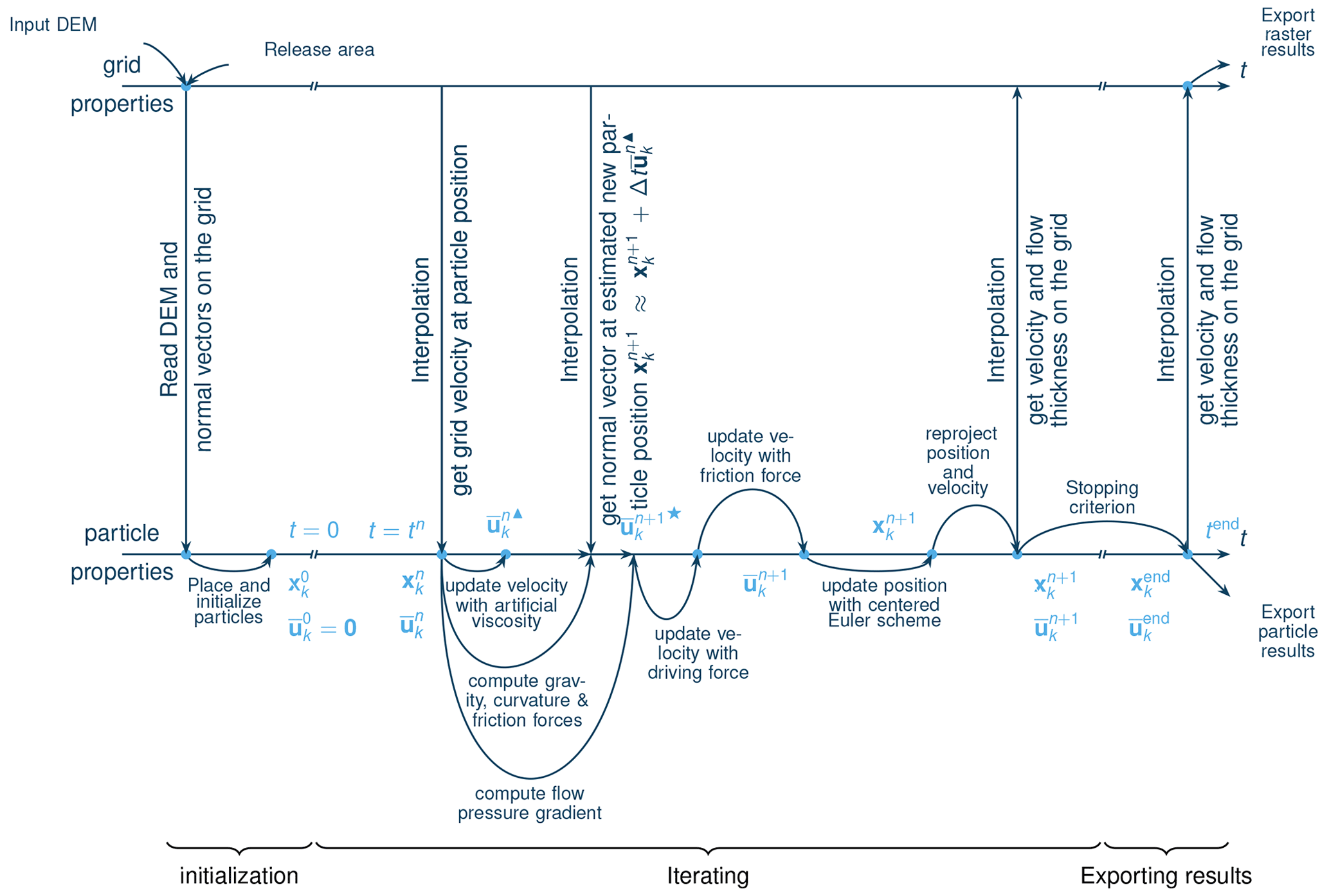
In this section, the numerical implementation and algorithm of the com1DFA module are described. The following sections are organized following the workflow used in the com1DFA code, which is also illustrated in Fig. 2. First, the release mass is discretized into particles and the grid is initialized. As a result of the partial differential equations considered and the time discretization used, stability issues might arise. Hence, artificial viscosity is added in order to ensure the stability of the solution. As a next step, driving forces (including curvature effects) are accounted for. Friction forces are taken into account subsequently in order to ensure proper starting and stopping behavior. Finally, a reprojection step is needed to ensure that particles lie on the topography and that particle velocities are tangential to the topography. For simplicity and because they are not considered in the verification tests in Sect. 5, entrainment and added resistance effects are not included in what follows. Additional information about entrainment or resistance forces is available in the theory section (https://docs.avaframe.org/en/theorypapercode/theoryCom1DFA.html#entrainment, last access: 5 October 2023) of the AvaFrame documentation.

4.1 Initialization

To start a simulation with com1DFA, input information about topography, material properties, and initial conditions is required. Topography is described by a DEM (digital elevation model) using the ESRI ASCII format. It supplies a grid of altitude values, preceded by a header with information about the number of data rows and columns, coordinates of the center or corner of the lower-left cell, the edge length of the quadratic cells, and the code used for missing values. The material is characterized by its density and some friction properties. The initial condition is given by release areas, polygons describing the initial material location, and the release thickness, in our case measured in the surface-normal direction. It is possible to provide several polygons with different initial thickness values.

Then the material is discretized into particles. The field of normal vectors to the surface is computed from the input DEM and the different grid fields are initialized. The details of the initialization process are given in the initialization section (https://docs.avaframe.org/en/theorypapercode/com1DFAAlgorithm.html#initialization, last access: 5 October 2023) of the AvaFrame documentation.

4.2 Numerical stability

Because the lateral shear force term was removed when deriving the model equations (because of its relative smallness, Gray and Edwards, 2014), Eq. (22) is hyperbolic. Hyperbolic systems have the characteristic of carrying discontinuities or shocks which will cause numerical instabilities. They would fail to converge if, for example, an Euler forward-in-time scheme is used (LeVeque, 1990). Several methods exist to stabilize the numerical integration of a hyperbolic system of differential equations. All add some upwinding in the discretization scheme. Some methods tackle this problem by introducing some upwinding in the discretization of the derivatives (Harten et al., 1983; Harten and Hyman, 1983). Others introduce some artificial viscosity (as in Monaghan, 1992), which is also implemented in com1DFA. The following artificial viscosity force acting on particle k is added to stabilize the momentum equation:

$$\begin{array}{ll}{\displaystyle }{\mathbf{F}}_k^{\text{visc}}=& {\displaystyle }-{\displaystyle \frac{\mathrm{1}}{\mathrm{2}}}{\mathit{\rho }}_{\mathrm{0}}{C}_{\text{Lat}}{A}_k^{\text{Lat}}{\left|\left|\mathit{d}{\stackrel{\mathrm{‾}}{\mathit{u}}}_k\right|\right|}^{\mathrm{2}}{\displaystyle \frac{\mathit{d}{\stackrel{\mathrm{‾}}{\mathit{u}}}_k}{\left|\left|\mathit{d}{\stackrel{\mathrm{‾}}{\mathit{u}}}_k\right|\right|}}\\ \text{(44)}& {\displaystyle }=& {\displaystyle }-{\displaystyle \frac{\mathrm{1}}{\mathrm{2}}}{\mathit{\rho }}_{\mathrm{0}}{C}_{\text{Lat}}{A}_k^{\text{Lat}}\left|\left|\mathit{d}{\stackrel{\mathrm{‾}}{\mathit{u}}}_k\right|\right|\mathit{d}{\stackrel{\mathrm{‾}}{\mathit{u}}}_k,\end{array}$$

where the velocity difference reads $\mathit{d}{\stackrel{\mathrm{‾}}{\mathit{u}}}_k={\stackrel{\mathrm{‾}}{\mathit{u}}}_k-{\widehat{\stackrel{\mathrm{‾}}{\mathit{u}}}}_k$ (${\widehat{\stackrel{\mathrm{‾}}{\mathit{u}}}}_k$ represents the averaged velocity of the neighbor particles and is practically the grid velocity interpolated at the particle position). C_Lat is a coefficient that controls the viscous force. It would be the equivalent of C_Drag in the case of the drag force. C_Lat is a numerical parameter that depends on the grid size.

In this expression, let ${\stackrel{\mathrm{‾}}{\mathit{u}}}_k^n$ be the velocity at the beginning of the time step and ${{\stackrel{\mathrm{‾}}{\mathit{u}}}_k^{n+\mathrm{1}}}^{▴}$ be the velocity after adding the numerical viscosity (Fig. 2). In the norm term $\left|\left|\mathit{d}{\stackrel{\mathrm{‾}}{\mathit{u}}}_k\right|\right|$ the particle and grid velocity at the beginning of the time step are used. This ensures explicit time discretization with respect to the norm $\left|\left|\mathit{d}{\stackrel{\mathrm{‾}}{\mathit{u}}}_k\right|\right|$ and $\widehat{\stackrel{\mathrm{‾}}{\mathit{u}}}$ in $\mathit{d}{\stackrel{\mathrm{‾}}{\mathit{u}}}_k$. In contrast, an implicit formulation is used in $\mathit{d}{\stackrel{\mathrm{‾}}{\mathit{u}}}_k$ because the new value of the velocity is used there. The artificial viscosity force now reads:

$$\begin{array}{}\text{(45)}& {\mathbf{F}}_k^{\text{visc}}=-{\displaystyle \frac{\mathrm{1}}{\mathrm{2}}}{\mathit{\rho }}_{\mathrm{0}}{C}_{\text{Lat}}{A}_k^{\text{Lat}}\left|\left|{\stackrel{\mathrm{‾}}{\mathit{u}}}_k^n-{\widehat{\stackrel{\mathrm{‾}}{\mathit{u}}}}_k^n\right|\right|\left({{\stackrel{\mathrm{‾}}{\mathit{u}}}_k^{n+\mathrm{1}}}^{▴}-{\widehat{\stackrel{\mathrm{‾}}{\mathit{u}}}}_k^n\right).\end{array}$$

Updating the velocity then gives

$$\begin{array}{}\text{(46)}& {{\stackrel{\mathrm{‾}}{\mathit{u}}}_k^{n+\mathrm{1}}}^{▴}={\displaystyle \frac{{\stackrel{\mathrm{‾}}{\mathit{u}}}_k^n+C_{\text{vis}}{\widehat{\stackrel{\mathrm{‾}}{\mathit{u}}}}_k^n}{\mathrm{1}+C_{\text{vis}}}},\end{array}$$

with

$$\begin{array}{}\text{(47)}& C_{\text{vis}}={\displaystyle \frac{\mathrm{1}}{\mathrm{2}}}{\mathit{\rho }}_{\mathrm{0}}{C}_{\text{Lat}}{A}_k^{\text{Lat}}\left|\left|{\stackrel{\mathrm{‾}}{\mathit{u}}}_k^n-{\widehat{\stackrel{\mathrm{‾}}{\mathit{u}}}}_k^n\right|\right|{\displaystyle \frac{\mathrm{\Delta }t}{m_k}}.\end{array}$$

This approach to stabilize the momentum equation (Eq. 30) is not optimal for different reasons. Firstly, it introduces a new coefficient C_vis, which is not a physical quantity and will require calibration. Secondly, it artificially adds a force that should be described physically. So it would be more interesting to take the physical force into account in the first place.

Potential solutions could be taking the physical shear force into account, using for example the μ(I)-rheology (Gray and Edwards, 2014; Baker et al., 2016). Another option would be to replace the artificial viscosity with a purely numerical artifact aiming to stabilize the equations, such as an SPH version of the Lax–Friedrichs scheme as presented in Ata and Soulaïmani (2005).

4.3 Curvature acceleration term

The last term of the particle momentum equation (Eq. 30), as well as the effective gravity g^eff, are the final terms to be discretized before the time integration. In both of these terms, the remaining unknown is the curvature acceleration term ${\stackrel{\mathrm{‾}}{\mathit{u}}}_k\cdot \frac{\mathrm{d}{\mathit{v}}_{\mathrm{3},k}}{\mathrm{d}t}$. Using the forward Euler time discretization for the temporal derivative of the normal vector v_3,k gives

$$\begin{array}{}\text{(48)}& {\left.{\displaystyle \frac{\mathrm{d}{\mathit{v}}_{\mathrm{3},k}}{\mathrm{d}t}}\right|}^n\approx {\displaystyle \frac{{\mathit{v}}_{\mathrm{3},k}^{n+\mathrm{1}}-{\mathit{v}}_{\mathrm{3},k}^n}{\mathrm{\Delta }t}}.\end{array}$$

${\mathit{v}}_{\mathrm{3},k}^n$ is a known quantity, the normal vector of the bottom surface at ${\mathit{x}}_k^n$ which is interpolated from the grid normal vector values at the position of the particle k at time tⁿ. ${\mathit{v}}_{\mathrm{3},k}^{n+\mathrm{1}}$ is unknown since ${\mathit{x}}_k^{n+\mathrm{1}}$ is not known yet, hence we estimate ${\mathit{x}}_k^{n+\mathrm{1}}$ based on the position ${\mathit{x}}_k^n$ and the velocity at tⁿ:

$$\begin{array}{}\text{(49)}& {\mathit{x}}_k^{n+\mathrm{1}}={\mathit{x}}_k^n+\mathrm{\Delta }t{{\stackrel{\mathrm{‾}}{\mathit{u}}}_k^{n+\mathrm{1}}}^{▴}.\end{array}$$

This position at tⁿ⁺¹ is projected onto the topography, and ${\mathit{v}}_{\mathrm{3},k}^{n+\mathrm{1}}$ can be interpolated from the grid normal vector values.

Note that the curvature acceleration term is needed to compute the bottom pressure (Eq. 24), which is used for the bottom friction computation and for the pressure gradient computation. The curvature acceleration term can lead to a negative value, which means detachment of the particles from the bottom surface. In com1DFA, surface detachment is not allowed, and if pressure becomes negative, it is set back to zero forcing the material to remain in contact with the topography.

4.4 Driving forces

Adding the driving forces is done after adding the artificial viscosity as described in Fig. 2. The velocity is updated as follows ( is the velocity after taking the driving force into account):

$$\begin{array}{}\text{(50)}& \begin{array}{rl}\textcolor{red}{}& ={{\stackrel{\mathrm{‾}}{\mathit{u}}}_k^{n+\mathrm{1}}}^{▴}+{\displaystyle \frac{\mathrm{\Delta }t}{m_k}}{\mathbf{F}}_k^{\text{drive}}={{\stackrel{\mathrm{‾}}{\mathit{u}}}_k^{n+\mathrm{1}}}^{▴}\\ & +{\displaystyle \frac{\mathrm{\Delta }t}{m_k}}\left(-m_k{g}_k^{\text{eff}}{\mathbf{\nabla }}_{s}h+m_k{\mathit{g}}_{\mathrm{s}}\right.\\ & \left.-m_k\left({{\stackrel{\mathrm{‾}}{\mathit{u}}}_k^{n+\mathrm{1}}}^{▴}\cdot {\left.{\displaystyle \frac{\mathrm{d}{\mathit{v}}_{\mathrm{3},k}}{\mathrm{d}t}}\right|}^n\right){\mathit{v}}_{\mathrm{3},k}^n\right),\end{array}\end{array}$$

where the flow thickness gradient term is computed using the SPH formulation in Eq. (32).

4.5 Friction forces

The friction force related to the bottom shear force needs to be taken into account in the momentum equation and the velocity needs to be updated accordingly. Friction force acts against motion, hence it only affects the magnitude of the velocity and cannot be a driving force (Mangeney-Castelnau et al., 2003). Moreover, the friction force magnitude depends on the particle state, i.e., whether it is flowing or at rest. If the velocity of the particle k is after adding the driving forces, adding the friction force leads, depending on the sign of $\frac{m_k\left|\left|\textcolor{red}{}\right|\right|}{\mathrm{\Delta }t}-{\left|\left|{\mathbf{F}}_k^{\text{fric}}\right|\right|}_{\text{max}}$, to

• $\left|\left|{\mathbf{F}}^{\text{fric}}\right|\right|={\left|\left|{\mathbf{F}}_k^{\text{fric}}\right|\right|}_{\text{max}}$ and ${\stackrel{\mathrm{‾}}{\mathit{u}}}_k^{n+\mathrm{1}}=\textcolor{red}{}\left(\mathrm{1}-\frac{\mathrm{\Delta }t}{m_k}\frac{{\left|\left|{\mathbf{F}}_k^{\text{fric}}\right|\right|}_{\text{max}}}{\left|\left|\textcolor{red}{}\right|\right|}\right)$, if $\frac{m_k\left|\left|\textcolor{red}{}\right|\right|}{\mathrm{\Delta }t}>{\left|\left|{\mathbf{F}}_k^{\text{fric}}\right|\right|}_{\text{max}}$

• $\left|\left|{\mathbf{F}}_k^{\text{fric}}\right|\right|\le {\left|\left|{\mathbf{F}}_k^{\text{fric}}\right|\right|}_{\text{max}}$, and the particle stops moving (${\stackrel{\mathrm{‾}}{\mathit{u}}}_k^{n+\mathrm{1}}=\mathrm{0}$) before the end of the time step if $\frac{m_k\left|\left|\textcolor{red}{}\right|\right|}{\mathrm{\Delta }t}\le {\left|\left|{\mathbf{F}}_k^{\text{fric}}\right|\right|}_{\text{max}}$.

This method prevents the friction force from becoming a driving force and nonphysically changing the direction of the velocity. This would lead to oscillations of the particles instead of stopping. Adding the friction force following this approach (Mangeney-Castelnau et al., 2003) allows the particles to start and stop flowing properly.

4.6 Reprojection

The last term in Eq. (30) (accounting for the curvature effects) adds a non-tangential component allowing the new velocity to lie in a different plane than the one from the previous time step. This enables the particles to follow the topography. Because the curvature term was only based on an estimation (see Sect. 4.3), the new particle position is not necessarily on the topography, and the new velocity does not necessarily lie in the tangent plane at this new position. Furthermore, in cases with a strong convex curvature and high velocities, the particles can theoretically be in a free-fall state (detachment), as mentioned in Sect. 2.5.1. Thus, com1DFA does not allow detachment of the particles, and the particles are forced to stay on the topography. This is a limitation of the model or method, which will lead to nonphysical behavior in special cases (material flowing over a cliff). In both of the previously mentioned cases, the particle positions are projected back onto the topography and the velocity direction is corrected to be tangential to the topography. The position reprojection is done using an iterative method that attempts to conserve the distance traveled by each particle between tⁿ and tⁿ⁺¹. The velocity reprojection changes the direction of the velocity, but its magnitude is conserved.

Figure 2 Dense-flow avalanche solver (com1DFA) workflow.

5 Model verification

In this section, the numerical implementation of the mathematical model is tested. We present different tests where, for specific conditions, a (semi-)analytical solution exists. The tests described here are implemented in the ana1Tests module from AvaFrame. In the first set of tests, the flow variable tests, we compare the temporal and spatial evolution of the flow thickness (h) and the thickness-integrated momentum flux ($h\stackrel{\mathrm{‾}}{\mathit{u}}$) of the com1DFA simulation results to a (semi-)analytical solution. With these tests, we aim to verify the numerical discretization and implementation of the solver and check the validity of the convergence criterion described in Sect. 3.6.

In the second test, the energy line test, we investigate global variables, such as mass-averaged position and kinetic energy, that are derived from the DFA simulations. This test is based on energy conservation considerations for simplified topographies. This allows us to verify the accuracy of the DFA simulations in terms of mass-averaged runout. All the tests presented and used in what follows are implemented and available in AvaFrame (both data and helper functions). All results and figures can be reproduced using the code available on the AvaFrame GitHub repository (https://github.com/avaframe/AvaFrame/tree/theoryPaperCode, last access: 5 October 2023).

5.1 Flow variable tests

Before performing the abovementioned similarity solution and dam break tests, it is necessary to describe the quantities that are compared and the measures that are used to assess the convergence, accuracy or precision of the numerical model. Both the flow thickness (h) and thickness-integrated flow momentum flux ($h\stackrel{\mathrm{‾}}{\mathit{u}}$) are used to compare the analytical solution to the simulation results. Two different deviation measures are used to quantify the deviation between a reference solution and the simulation result on a domain (one- or two-dimensional). The first is based on the ℒ_max norm (uniform norm), and the second is based on the Euclidean norm (ℒ₂ norm). Let f_num be the numerical solution and f_ref the reference solution defined on a domain Ω. The local deviation is defined by $\mathcal{E}\left(x\right)=f_{\text{num}}\left(x\right)-f_{\text{ref}}\left(x\right)$, and the global deviation is defined by the following terms.

• The uniform norm (ℒ_max) measures the largest absolute value of the deviation ℰ on Ω:

  $${\mathcal{L}}_{\text{max}}\left(\mathcal{E}\right)=\underset{x\in \mathrm{\Omega }}{sup}\left(\right|\mathcal{E}\left(x\right)\left|\right).$$

  This norm is applied to one- or two-dimensional results. It can also be normalized by dividing the uniform norm of the deviation by the uniform norm of the reference. In this case we refer to the relative deviation:

  $$\mathcal{R}{\mathcal{L}}_{\text{max}}={\displaystyle \frac{{\mathcal{L}}_{\text{max}}\left(\mathcal{E}\right)}{{\mathcal{L}}_{\text{max}}\left(f_{\text{ref}}\right)}}.$$

• The Euclidean norm (ℒ₂ norm) gives an overall measure of the deviations

  $${\mathcal{L}}_{\mathrm{2}}\left(\mathcal{E}\right)=\underset{x\in \mathrm{\Omega }}{\int }{\left|\left|\mathcal{E}\left(x\right)\right|\right|}^{\mathrm{2}}\mathrm{d}x.$$

  It is useful to normalize the norm of the deviation either by dividing with the norm of the reference solution:

  $$\mathcal{R}{\mathcal{L}}_{\mathrm{2}}={\displaystyle \frac{{\mathcal{L}}_{\mathrm{2}}\left(\mathcal{E}\right)}{{\mathcal{L}}_{\mathrm{2}}\left(f_{\text{ref}}\right)}}$$

  or by the measure of the interval (${\mathcal{L}}_{\mathrm{2}}\left(\mathrm{1}\right)={\int }_{x\in \mathrm{\Omega }}\mathrm{d}x$):

  $$\mathcal{R}\mathcal{S}{\mathcal{L}}_{\mathrm{2}}=\sqrt{{\displaystyle \frac{{\mathcal{L}}_{\mathrm{2}}\left(\mathcal{E}\right)}{{\mathcal{L}}_{\mathrm{2}}\left(\mathrm{1}\right)}}}.$$

  The first normalization approach will give a relative deviation, whereas the second will give an average deviation of f on Ω.

5.1.1 Similarity solution test

The similarity solution is one of the few cases where a semi-analytic solution is available for solving the thickness-integrated equations. This makes it very useful for validating the implementation of dense-flow avalanche numerical methods (here com1DFA). In this problem, we consider an avalanche governed by a dry-friction law (Coulomb friction) flowing down an inclined plane. The release mass is initially distributed in an ellipse (diameters of length L_x and L_y) with a parabolic thickness shape (H in the middle). This mass is released at t=0 and flows down the inclined plane, as illustrated in Fig. 3a for the initial time step and at some later time t. This semi-analytic solution can be derived under the following assumptions. First, the ratio $\mathit{ϵ}=H/L$ of flow thickness over spatial extent in flow and cross-flow direction should be smaller than 1. Second, the slope angle must be larger than the bed friction angle. Third, the solution is assumed to retain the symmetry properties of the initial configuration relative to the moving center of mass. The full description of the conditions and assumptions, as well as the derivation of the solution, is presented in detail by Hutter et al. (1993). The term semi-analytic is used here because the method enables us to transform the PDE (partial differential equation) of the problem into an ODE (ordinary differential equation) using a similarity analysis method. The ODE can be solved with much less effort, e.g., using an explicit fourth-order Runge–Kutta scheme.

This test is implemented in the ana1Tests module of AvaFrame, which offers functions to compute the semi-analytic solution, compare it to the output from the DFA computational module, and visualize the results.

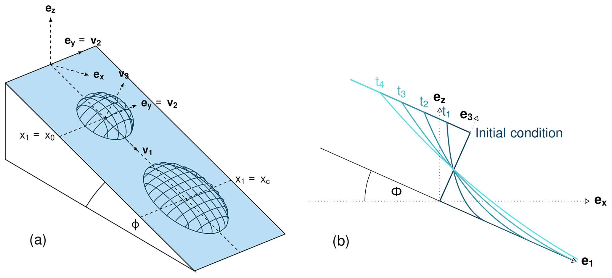
Figure 3 Flow variable test setups. (a) Similarity solution showing a 3D view of the material on the inclined plane at t=0 (center located in x₁=x₀) and at a general time t (center located in x₁=x_c). The footprint of the material on the inclined plane at the initial time is an ellipse of principal axes L_x and L_y, the thickness follows a parabolic distribution, with the maximum thickness of H in the middle of the ellipse and 0 on the edge. (b) Dam break showing a 2D view of the material on the inclined plane (profile in flow direction) at t=0 and for different t>0.

5.1.2 Dam break test

The dam break test is the second test for which an analytical solution of the thickness-integrated equations is known. In this test, we also consider an avalanche governed by a dry-friction law (Coulomb material), released from rest on an inclined plane (see Fig. 3b). In the case of a thickness-integrated model as derived by Savage and Hutter (e.g., in Hutter et al., 1993), an analytical solution exists under the assumption of shallowness of the flow. Furthermore, the friction angle has to be smaller than the slope of the inclined plane. This test, in contrast to the similarity solution test, focuses on the very early stages of the flow and not on the evolution over time and lateral spreading. The derivation of the dam break solution is described in Faccanoni and Mangeney (2013) and corresponds to a Riemann problem. It has the following initial conditions:

$$\begin{array}{}\text{(51)}& (h,\mathit{u})(x,t=\mathrm{0})=\left\{\begin{array}{ll}(h_{\mathrm{0}},\mathbf{0}),& \text{if }x\le \mathrm{0}\\ (\mathrm{0},\mathbf{0}),& \text{if }x>\mathrm{0}.\end{array}\right.\end{array}$$

The dam break assumes an invariance in the y direction, which is achieved using a wide enough domain in the y direction so that lateral effects can be neglected.

5.1.3 Results

DFA simulations are computed using the com1DFA module in AvaFrame varying the different numerical parameters listed in Table 1. The range of α values (called “aPPK” in the code and figures) is determined by the convergence criterion (Eq. 43). The SPH kernel radius r_kernel (called “sphKernelRadius” in the code and figures) is varied around 5 m, which is the raster cell size value currently used for operational hazard mapping in Austria. The tested values of n_ppk0 (called “nPPK0” in the code and figures) and C_time (called “cMax” in the code and figures) are listed in Table 1. A large n_ppk0 and small C_time lead to very long computation time, which makes these values unrealistic and impractical to use. Instructions on how to reproduce the results presented below are provided in the Supplement.

Table 1 Parameter variation used to study convergence of the DFA simulation solution for both similarity solution and dam break test ( the parameters used for the figures presented in this article are given in bold).

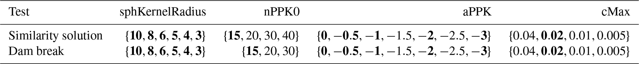
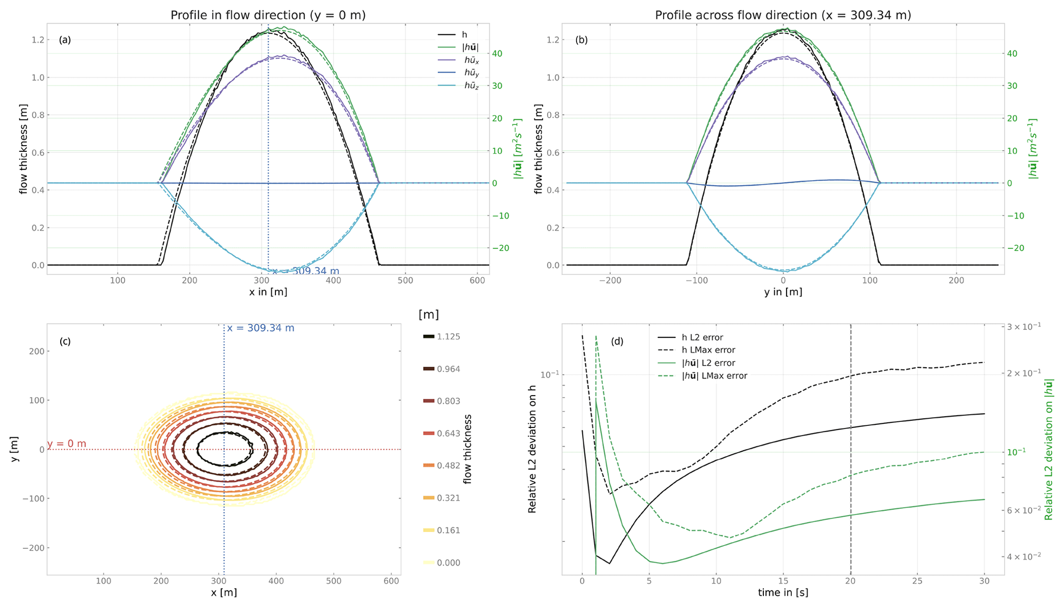
Figure 4 Comparison of the analytical (dashed lines) and numerical (solid lines) solution for the similarity solution test case at t=20.04 s. Panel (a) shows the profile in the flow direction (along the x axis), whereas (b) shows the profiles across flow direction (along the y axis). Panel (c) provides a top view of the flow thickness (flow thickness contour lines). Panel (d) shows the time evolution of the deviation (both ℛℒ_max and ℛℒ₂) on flow thickness h and momentum $\left|\left|h\stackrel{\mathrm{‾}}{\mathit{u}}\right|\right|$ between the analytic and numerical solutions (r_kernel=3 m, $\mathit{\alpha }=-\mathrm{3}$, $n_{\text{ppk}}^{\mathrm{0}}=\mathrm{15}$ and C_time=0.02 s m⁻¹). Large relative error values are mainly connected to differences in the generally small upstream values in flow direction. The vertical dashed line in (d) marks the time at which data in panels (a), (b), and (c) are shown. Results of the similarity solution test with the standard parameters are shown in the Supplement.

For both of the tests, the numerical schemes to apply friction and the method used to compute the SPH gradient are crucial for obtaining a proper starting and stopping behavior of the flow. Some intermediate developments showed that adding the friction with methods differing from as the one presented here and computing the SPH gradient without taking the slope inclination into account leads to unsatisfactory results. This is why the friction force is added as described in Sect. 4.5 and the SPH force is computed as described in Appendix B2. In what follows, artificial viscosity is added with C_Lat=10) in the similarity solution test, which stabilizes the solution without degrading the match with the semi-analytic solution. For the dam break test, adding artificial viscosity has a negative impact on the solution and the following results were produced with no artificial viscosity (C_Lat=0).

Figure 4 shows an example where a DFA simulation is compared to the semi-analytical solution of the similarity solution test case. The chosen parameters for this example are r_kernel=3 m, $\mathit{\alpha }=-\mathrm{3}$, $n_{\text{ppk}}^{\mathrm{0}}=\mathrm{15}$ and C_time=0.02 s m⁻¹ and correspond to the most accurate of the simulations presented here. The reader can find the results of the similarity solution test with the standard parameters in the Supplement. Figure 4a and b show the flow thickness and momentum profiles in and across flow direction after 20 s of flow. Figure 4d shows the evolution of the ℛℒ₂ and ℛℒ_max deviation with time. The deviation at the initial time step (t=0 s) is rather high (this is related to the random process to initialize the particles in the simulation) and then quickly decreases after a few seconds of simulation due to the reorganization of the particles. The deviation then increases again as the numerical inaccuracies accumulate. When varying the numerical parameters in the DFA simulations (according to Eq. 42), the computed ℒ₂ deviations between DFA results and the semi-analytical solution decrease (see Fig. 5). In Fig. 6, the comparison between a DFA simulation and the analytical solution of the dam break test is shown for flow thickness, flow velocity and momentum at t=15 s (upper panel). Figure 6d shows a top view of the flow colored by flow thickness. This panel also shows the domain on which the deviation between analytical and numerical solution is computed. Figure 6e shows the relative deviations ℛℒ₂ and ℛℒ_max on flow thickness and momentum. The same behavior as for the similarity solution test is observed regarding the time evolution of the deviation. Computation was done with r_kernel=3 m, $\mathit{\alpha }=-\mathrm{3}$, $n_{\text{ppk}}^{\mathrm{0}}=\mathrm{15}$ and C_time=0.02 s m⁻¹. The reader can find the results of the similarity solution test with the standard parameters in the Supplement.

Results from both the similarity solution tests and the dam break test validate the convergence criterion from Ben Moussa and Vila (2000). Indeed, with an α exponent smaller than −1, decreasing the SPH kernel radius and varying the other parameters according to Eq. (42) leads to a decrease in the deviation, whereas for larger exponents, $\mathit{\alpha }=-\mathrm{0.5}$ for both tests or α=0 for the dam break test (Fig. 7), the deviation decreases only slightly or even increases. Moreover, it is observed (not shown in the figure) that decreasing the time step (decreasing the C_max parameter) with all other parameters fixed leads to a decreasing deviation. Finally, for these two specific cases, DFA simulation results converge towards the semi-analytical or analytical solution.

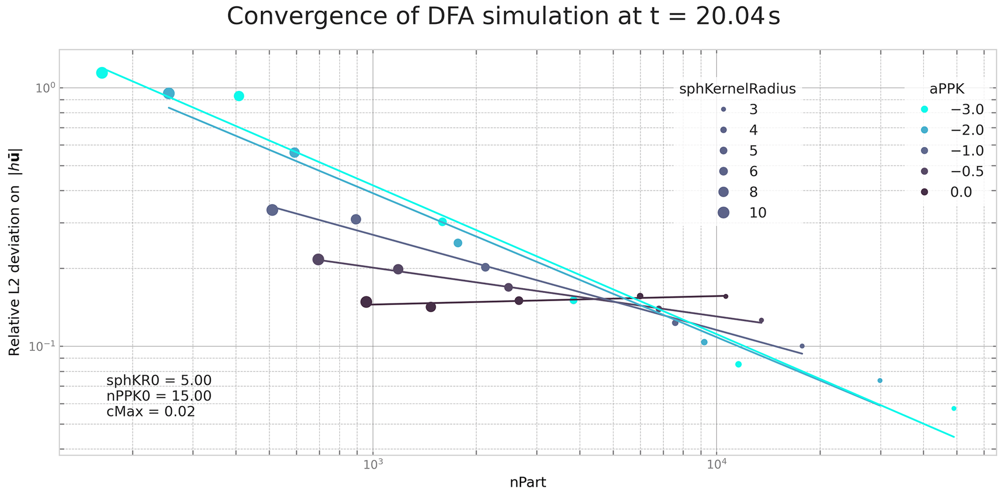
Figure 5 ℛℒ₂ deviation of flow momentum in the similarity solution test case for different α exponents and SPH kernel radii r_ppk. Other parameters are kept fixed (reference kernel radius $r_{\text{ppk}}^{\mathrm{0}}=\mathrm{5}$ m, time constant C_time, and reference number of particles per kernel radius $n_{\text{ppk}}^{\mathrm{0}}$). Due to the reference kernel radius all points for r_ppk=5 m are identical. The colored lines are added to give an idea of the convergence speed trend associated with each α scenario. The decrease in the deviation is stronger for lower α exponents, and no or little decrease is observed for α=0 or $\mathit{\alpha }=-\mathrm{0.5}$.

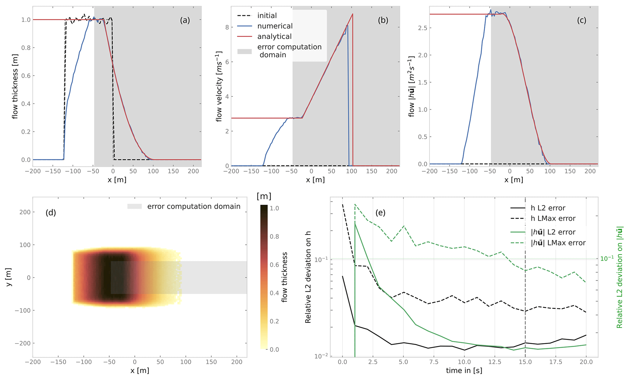
Figure 6 Comparison of the analytical and numerical solution for the dam break test case at t=15.0 s. Thee top panels show flow thickness (a), velocity (b), and momentum profiles (c) in flow direction. Panel (d) provides a top view of the flow thickness. The gray-shaded rectangle represents the domain on which the deviations are computed. Panel (e) shows the time evolution of the deviation (both ℛℒ_max and ℛℒ₂) on flow thickness h and momentum $\left|\left|h\stackrel{\mathrm{‾}}{\mathit{u}}\right|\right|$ between the analytic and numerical solutions (r_kernel=3 m, $\mathit{\alpha }=-\mathrm{3}$, $n_{\text{ppk}}^{\mathrm{0}}=\mathrm{15}$ and C_time=0.02 s m⁻¹). The vertical dashed line in (e) marks the time at which data in the other panels are shown.

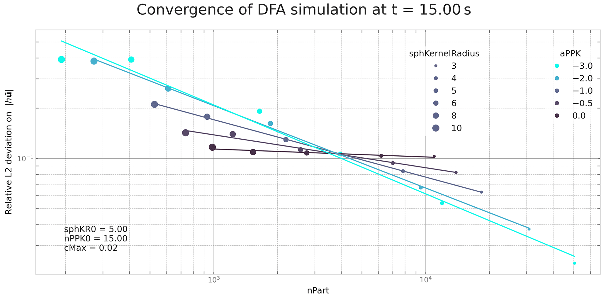
Figure 7 ℛℒ₂ deviation in flow momentum in the dam break case for different α exponents and SPH kernel radii r_ppk. Other parameters are kept fixed (reference kernel radius $r_{\text{ppk}}^{\mathrm{0}}=\mathrm{5}$ m, time constant C_time, and reference number of particles per kernel radius $n_{\text{ppk}}^{\mathrm{0}}$). Due to the reference kernel radius, all points for r_ppk=5 m are identical. The colored lines are added to give an idea of the convergence speed trend associated with each α scenario. One can observe that the decrease in deviation is stronger for lower α exponents and that no or little decrease is observed for α=0 or $\mathit{\alpha }=-\mathrm{0.5}$.

5.2 Energy and runout testing

The energy line test compares the results of the com1DFA simulation to a geometrical solution derived from the total energy of the system. Solely considering Coulomb friction, this solution is motivated by the first principle of energy conservation along a simplified topography. In this case, the friction force only depends on the slope angle. The analytical runout is the intersection of the path profile with the geometrical line (α line) defined by the friction angle α. From the geometrical line it is also possible to extract information about the mass-averaged flow velocity at any time or position along the path profile (see example in Fig. 9). For the detailed theory of this test, please refer to Appendix A.

In this test, we use the α line to evaluate the DFA simulation. Computing the mass-averaged path profile for the particles (each particle corresponding to a material point) in the simulation and comparing it to the α line allows us to compute four error indicators. Fig. A1 illustrates the concept.

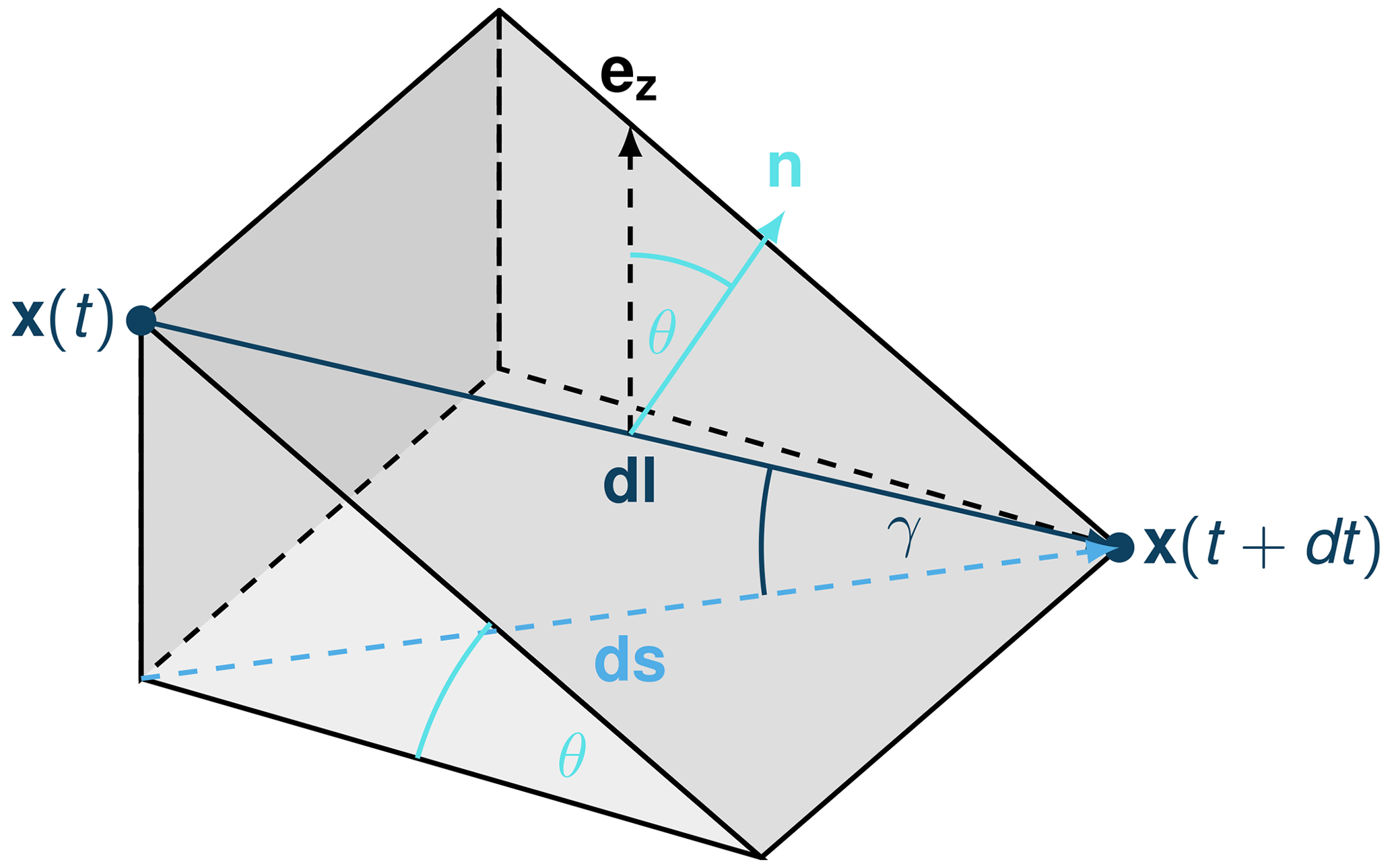
Figure 8 Example of trajectory where the steepest descent path hypothesis fails. The mass point is traveling from x(t) to x(t+dt). The slope angle θ and travel angle γ are also illustrated. Here $({\mathit{e}}_z\cdot \mathit{n})\mathrm{d}l=\cos \mathit{\theta }\frac{\mathrm{d}s}{\cos \mathit{\gamma }}\ne \mathrm{d}s$.

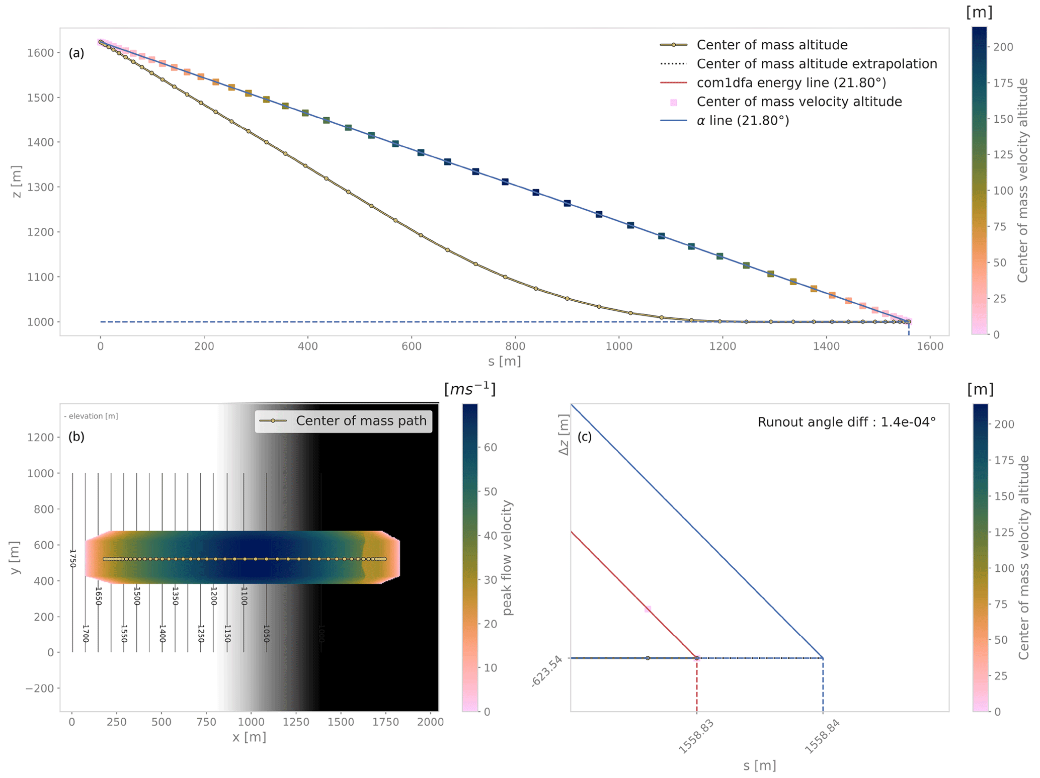
Figure 9 Energy line test for an inclined plane smoothly transitioning to a horizontal plane with particles following Coulomb friction and not subject to pressure forces. All conditions for the energy line test to be applicable are satisfied, and the geometrical solution can be used as reference to compute the numerical error (here less than 10⁻² m and 10^−4∘). Panel (a) shows the center of mass profile, which is indicated in the top view of peak flow velocity in panel (b). Panel (c) shows a zoomed-in view of the lower end of the profile.

The first three are related to the analytical runout point defined by the intersection between the α line and the mass-averaged path profile. The last one is related to the velocity.

• The horizontal distance between the analytical runout point and the end of the path profile defines the ${\mathit{ϵ}}_{\mathrm{s}}={\stackrel{\mathrm{‾}}{s}}_{\mathit{\gamma }}-{\stackrel{\mathrm{‾}}{s}}_{\mathit{\alpha }}$ error in meters.

• The vertical distance between the analytical runout point and the end of the path profile defines the ${\mathit{ϵ}}_z={\stackrel{\mathrm{‾}}{z}}_{\mathit{\gamma }}-{\stackrel{\mathrm{‾}}{z}}_{\mathit{\alpha }}$ error in meters.

• The runout angle difference between the α line angle and the DFA simulation runout line defines the ${\mathit{ϵ}}_{\mathit{\alpha }}=\mathit{\gamma }-\mathit{\alpha }$ runout angle error.

• The root-mean-square error (RMSE) between the α line and the DFA simulation energy points defines an error in the velocity altitude $\frac{\stackrel{\mathrm{‾}}{v^{\mathrm{2}}}}{\mathrm{2}g}$.

5.2.1 Limitations and applicability

It is essential to state where the assumptions of this test hold. One of the important hypotheses for the energy solution is that the inclination of the material point trajectory is equal to the slope angle of the surface, i.e., where $\mathrm{d}l=\frac{\mathrm{d}s}{\cos \mathit{\theta }}$. If this hypothesis fails, e.g., due to a particle trajectory deviating from the steepest slope direction, as illustrated in Fig. 8, it is impossible to derive the analytical energy solution. In the 3D case, the distance traveled by the particles reads $\left|\right|\mathrm{d}l\left|\right|=\frac{\mathrm{d}s}{\cos \mathit{\gamma }}$, where γ is the angle between the dl vector and the horizontal plane, which can differ from the slope angle θ (γ≤θ). Here the energy solution is not the solution to the problem and hence cannot be used as reference. In this case, it would not be possible to distinguish what deviation is caused by the numerical error or because of the hypothesis being violated.

The α line can be used to study the effect of terms such as curvature acceleration, artificial viscosity, or pressure gradients. For example, the curvature acceleration modifies the friction term, depending on topography curvature and particle velocity, leading to a mismatch between the energy solution and the DFA simulation. Figure 10 shows this curvature effect. The topography considered here is an inclined plane that smoothly transitions into a horizontal plane, meaning that curvature only occurs in the transition part. The energy line test for this case shows that there is added dissipation only in the transition part, seen by squares not following the α line. Once all particles have reached the horizontal plane, the squares follow the α line again (with a shift in s coordinate or, perhaps more intuitively, in the z coordinate).

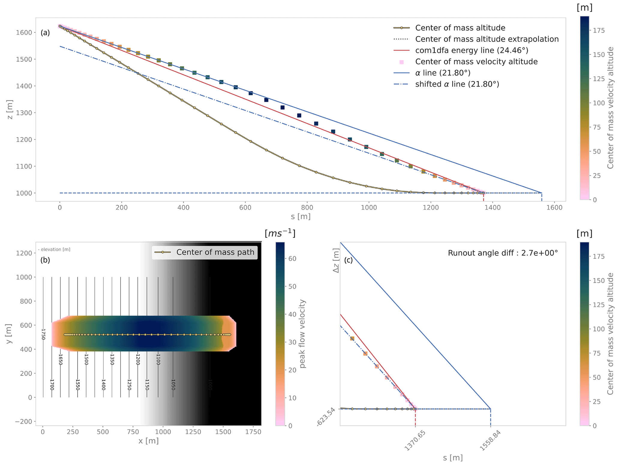
Figure 10 Energy line test for an inclined plane smoothly transitioning to a horizontal plane with particles following Coulomb friction, not subject to pressure forces but taking curvature acceleration into account. The geometrical solution and the numerical solution match on the inclined plane and horizontal parts and differ on the curved part. This shows the effect of curvature on the runout (decrease of runout because of the added friction due to curvature). Panel (a) shows the center of mass profile, which is indicated in the top view of peak flow velocity in panel (b). Panel (c) shows a zoom-in to the lower end of the profile.

Finally, the effects of the pressure force can be studied. For example, with this test it can be shown that adding the pressure forces does not influence the simulation runout (not shown here). This can be explained by the fact that pressure forces do not dissipate any energy and hence should not affect the energy balance. However, pressure forces lead to particle trajectories that do not necessarily follow the steepest direction, which means that the fundamental hypothesis illustrated in Fig. 8 is not satisfied.

5.2.2 Grid orientation effect

The energy line test previously described is also used to test whether the numerical method implemented in com1DFA performs independently of the grid orientation. Indeed we saw in Sect. 3.1 that com1DFA uses a regular grid to update some variables such as flow thickness or flow velocity. In order to quantify the effect of the grid orientation on the simulation results, we perform tests where grid orientation is changed while keeping the grid cell size and topography the same. In the Supplement, we show two examples where we consider a parabolic slope, i.e., the topography varies only in one direction, and a bowl shape, i.e., the topography with a rotational symmetry about its center. The main axis of the flow is not always aligned with the grid, and we provide three cases. First, a 0^∘ case in which the slope is invariant in the y direction (main flow direction aligned with the grid). Second, a 225^∘ case, with the slope being invariant in a direction angled 225^∘ from the y direction (main flow direction aligned with the grid diagonal). Third, a 120^∘ case meaning that the slope is invariant in a direction angled 120^∘ from the y direction (main flow direction is neither aligned with the grid nor with the grid diagonal). For each of these test cases, two simulations are performed, i.e., with or without pressure gradients. The results of these tests and the instructions on how to reproduce them are provided in the Supplement. The results are very satisfying. The runout distances differ by only a few centimeters between the 0, 120, and 225^∘ cases. This is of the same order of magnitude as the numerical errors computed with the energy line tests. This proves the rather low dependence of the simulation results on the grid orientation.

6 Conclusions

The presented com1DFA module within the open-source simulation framework AvaFrame is aimed at and developed for the simulation of avalanches with flow or a mixed form of movement. These may mostly be classified as A2B7C1D-E7F7G1H7J1 according to the morphological classification code (International Association of Hydrological Sciences. International Commission on Snow and Ice, 1981). Effects of snow entrainment or additional sources of resistance can be included. The corresponding theoretical background is not described in this publication but is available in the AvaFrame online documentation (Oesterle et al., 2022).

The default setup of the module targets very large to extremely large avalanches of catastrophic intensity, corresponding to avalanches of size 4–5 of the European Avalanche Warning Service (EAWS) size classification or a 150-year return period in the case of Austrian hazard mapping (Johannesson et al., 2009). Additional calibrated parameter sets for small- and medium-sized avalanches and wet-snow avalanches (albeit experimental) are also provided within the framework. However, these are exclusively optimized on a subset of Austrian test cases. Other types of avalanches, such as powder snow avalanches or similar, are unsuitable applications for the com1DFA module.

Com1DFA is based on the slope-normal thickness integration of the mass and momentum conservation equations, which are solved with a mixed particle–grid method. Particles are used to track mass and to compute the pressure forces following a smooth particle hydrodynamics (SPH) approach adapted to the special case of steep terrain. An underlying Eulerian grid is used to compute the flow thickness from the distribution of the particles. Velocity is also interpolated from the particles to the grid in order to compute the stabilizing artificial viscosity term. Physical starting and stopping behavior is ensured by considering differences in the friction force, whether the material is flowing or at rest. A time–space criterion ensuring the convergence of the implemented numerical method is provided. Of course limitations and assumptions exist, one of the main ones being the assumption of a moderately curved surface. For currently used resolutions of topographies (about 5–10 m at the time of writing) terrain features remain relatively smooth, but this already requires forcing of particles to stay on the topography. For potential higher-resolution applications in the future, this assumption needs to be re-evaluated.

To verify the numerical implementation of com1DFA, we apply a series of tests separated into two categories. Flow variable tests, i.e., similarity solution and dam break tests, are used for checking the proper spatiotemporal evolution of flow thickness and velocity. Runout testing checks the accuracy of global variables such as center-of-mass runout and kinetic energy. The tests show the validity of the chosen time–space criterion, as well as the accuracy and precision of the com1DFA numerical solution.

Note that the computational efficiency of the com1DFA module is not a topic in this article since simulations with the standard setup compute within seconds to minutes on current computer hardware. To achieve better computational efficiency, we implemented parallel execution of multiple serial simulations. However, topics like computational efficiency, further in-depth testing, and application to real topographies will be treated in future publications.

Current and future potential improvements to com1DFA include topics such as the improvement of entrainment and detrainment (e.g., concerning forests), a more numerically sound representation of dams and walls, or a probabilistic approach to uncertainties. These topics will need both conceptual developments and numerical improvements, but some are already being tackled. Possible applications to other types of gravitational mass flows might also be an exciting development, but our current focus lies on snow avalanches. However, since AvaFrame is an open-source framework, we invite everyone to use the presented modules and welcome feedback and contributions, regardless of the topic.

Appendix A: Theory: energy line test

The conservation of energy for a material point (block model) flowing downslope from point O to point B reads as follows (assuming only Coulomb friction):

$$\begin{array}{ll}{\displaystyle }{E}_{\mathrm{B}}^{\text{tot}}-E_{\mathrm{O}}^{\text{tot}}& {\displaystyle }=E_{\mathrm{B}}^{\text{kin}}+E_{\mathrm{B}}^{\text{pot}}-(E_{\mathrm{O}}^{\text{kin}}+E_{\mathrm{O}}^{\text{pot}})=\underset{\mathrm{O}}{\overset{\mathrm{B}}{\int }}\mathit{\delta }{E}_{\text{fric}}\\ {\displaystyle }& {\displaystyle }={\displaystyle \frac{\mathrm{1}}{\mathrm{2}}}m{v}_{\mathrm{B}}^{\mathrm{2}}+mg{z}_{\mathrm{B}}-{\displaystyle \frac{\mathrm{1}}{\mathrm{2}}}m{v}_{\mathrm{O}}^{\mathrm{2}}-mg{z}_{\mathrm{O}}\\ \text{(A1)}& {\displaystyle }& {\displaystyle }=\underset{\mathrm{O}}{\overset{\mathrm{B}}{\int }}{\mathbf{F}}_{\text{fric}}\cdot \mathit{d}\mathit{l}=-\underset{\mathrm{O}}{\overset{\mathrm{B}}{\int }}\mathit{\mu }mg({\mathit{e}}_z\cdot \mathit{n})\mathrm{d}l,\end{array}$$

where δE_fric is the energy dissipation due to friction, n the normal vector to the slope surface, and dl is the elementary vector on the path profile traveled by the material point between O and B. The vertical component of the normal vector reads ${\mathit{e}}_z\cdot \mathit{n}=\cos \mathit{\theta }$, where θ is the slope angle. Here, m represents the mass of the material point, g the gravity, μ=tan α the friction coefficient and friction angle, z the elevation, and v the velocity of the material point. Note that in the 2D case, $\mathrm{d}l=\frac{\mathrm{d}s}{\cos \mathit{\theta }}$ is only true if the inclination of the material point trajectory is equal to the slope inclination, i.e., the material point is flowing in the steepest slope direction. Now considering O as the origin position (s_O=0 and v_O=0) leads to the following simplification:

$$\begin{array}{}\text{(A2)}& {\displaystyle }\textcolor{red}{}\end{array}$$

Speaking in terms of altitude, the energy conservation equation can be rewritten (the subscript B is dropped):

$$\begin{array}{}\text{(A3)}& z_{\mathrm{O}}=z+{\displaystyle \frac{v^{\mathrm{2}}}{\mathrm{2}g}}+\tan \mathit{\alpha }.\end{array}$$

Considering a system of material points flowing down a slope with Coulomb friction, we can sum the previous equation (Eq. A3) of each material point after weighting it by its mass. This leads to the mass-averaged energy conservation equation:

$$\begin{array}{}\text{(A4)}& {\stackrel{\mathrm{‾}}{z}}_{\mathrm{O}}=\stackrel{\mathrm{‾}}{z}+{\displaystyle \frac{\stackrel{\mathrm{‾}}{v^{\mathrm{2}}}}{\mathrm{2}g}}+\stackrel{\mathrm{‾}}{s}\tan \mathit{\alpha },\end{array}$$

where the mass-averaged value $\stackrel{\mathrm{‾}}{a}$ of a quantity a is (k indicates the points indices) as follows:

$$\begin{array}{}\text{(A5)}& \stackrel{\mathrm{‾}}{a}={\displaystyle \frac{{\sum }_k{m}_k{a}_k}{{\sum }_k{m}_k}}.\end{array}$$

In this way, we can define the center-of-mass path $(\stackrel{\mathrm{‾}}{x},\stackrel{\mathrm{‾}}{y})$ and the center-of-mass path profile $(\stackrel{\mathrm{‾}}{s},\stackrel{\mathrm{‾}}{z})$. The mass-averaged quantities also follow the same energy conservation law when expressed in terms of altitude. This result is illustrated in Fig. A1b and applies to both the material point equation (Eq. A3) and the mass-averaged energy conservation equation (Eq. A4). The light blue line in Fig. A1b is obtained by evaluating the mass-averaged energy conservation (Eq. A4) at the final time (t_end) and position ($({\stackrel{\mathrm{‾}}{s}}_{\text{end}}$, ${\stackrel{\mathrm{‾}}{z}}_{\text{end}})$), where v²=0. This leads to the α line (also called energy line) equation:

$$\begin{array}{}\text{(A6)}& \stackrel{\mathrm{‾}}{z}={\stackrel{\mathrm{‾}}{z}}_{\mathrm{O}}-\stackrel{\mathrm{‾}}{s}\tan \mathit{\alpha }.\end{array}$$

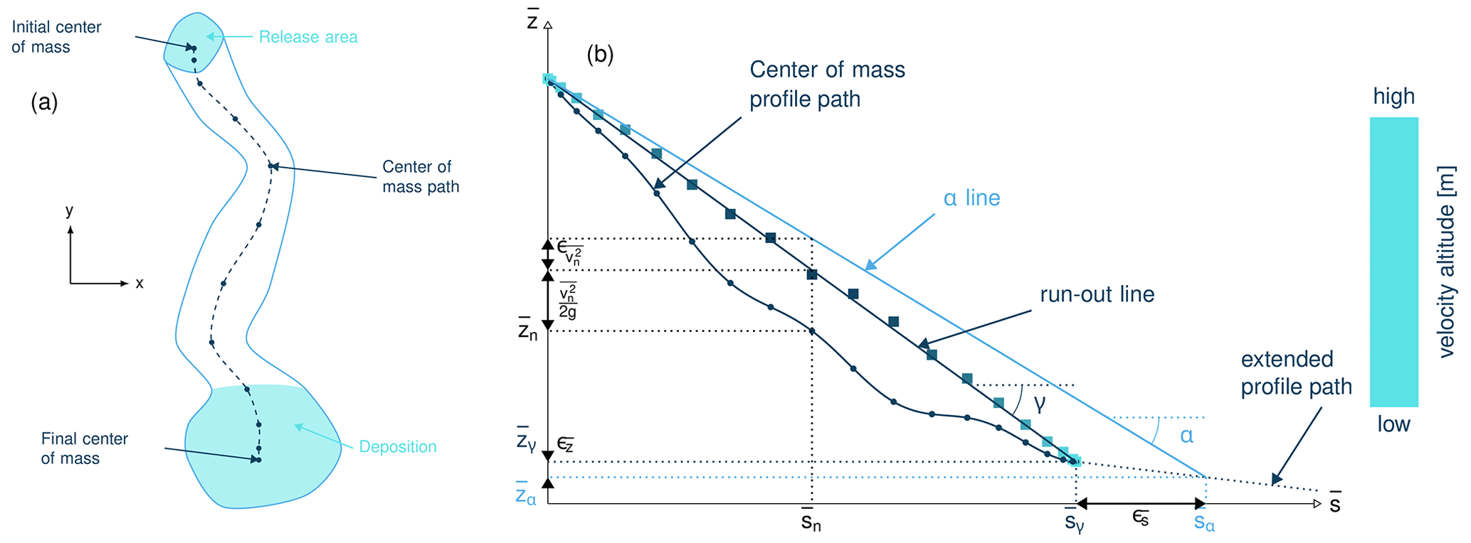
Figure A1 Panel (a) shows a top-down view of the avalanche simulation and extracted path. Panel (b) shows a simulation path profile (dark blue curve and dots) with the runout line (dark blue line and velocity altitude squares), α line, and runout error indicators (ϵ_s and ϵ_z)

Appendix B: SPH pressure gradients

The SPH method used in shallow-water equations is in most applications applied on a horizontal surface. The theoretical development on a horizontal plane is described in Appendix B1. The dense-flow avalanche model described in this paper should be expressed on the bottom surface, which is not necessarily horizontal. The SPH gradient computation development is detailed in Appendix B2.

B1 Standard method

Let us start with the computation of the gradient of a scalar function $f:{\mathbb{R}}^{\mathrm{2}}\to \mathbb{R}$ on a horizontal plane. Let $P_k={\mathit{x}}_k=(x_{k,\mathrm{1}},x_{k,\mathrm{2}})$ and $Q_l={\mathit{x}}_l=(x_{l,\mathrm{1}},x_{l,\mathrm{2}})$ be two points in ℝ² defined by their coordinates in the Cartesian coordinate system $(P_k,{\mathit{e}}_{\mathrm{1}},{\mathit{e}}_{\mathrm{2}})$. ${\mathit{r}}_{kl}={\mathit{x}}_k-{\mathit{x}}_l$ is the vector from Q_l to P_kl. Now consider the kernel function W:

$$\begin{array}{}\text{(B1)}& W:{\mathbb{R}}^{\mathrm{2}}\times {\mathbb{R}}^{\mathrm{2}}\times \mathbb{R}\to \mathbb{R},(P_k,Q_l,r_{\mathrm{0}})\mapsto W(P_k,Q_l,r_{\mathrm{0}}).\end{array}$$

r₀∈ℝ is the smoothing kernel length (or radius). In the case of the spiky kernel, W reads as follows (2D case):

$$\begin{array}{ll}\text{(B2)}& {\displaystyle }{W}_{kl}=& {\displaystyle }W({\mathit{x}}_k,{\mathit{x}}_l,r_{\mathrm{0}})=W({\mathit{x}}_k-{\mathit{x}}_l,r_{\mathrm{0}})=W({\mathit{r}}_{kl},r_{\mathrm{0}}){\displaystyle }=& {\displaystyle \frac{\mathrm{10}}{\mathit{\pi }{r}_{\mathrm{0}}^{\mathrm{5}}}}\left\{\begin{array}{ll}(r_{\mathrm{0}}-\left|\left|{\mathit{r}}_{kl}\right|\right|{)}^{\mathrm{3}},& \mathrm{0}\le \left|\left|{\mathit{r}}_{kl}\right|\right|\le r_{\mathrm{0}}\\ \mathrm{0},& r_{\mathrm{0}}<\left|\left|{\mathit{r}}_{kl}\right|\right|.\end{array}\right.\end{array}$$

$\left|\left|{\mathit{r}}_{kl}\right|\right|=\left|\left|{\mathit{x}}_k-{\mathit{x}}_l\right|\right|$ is the distance between particles k and l, and r₀ is the smoothing length. Using the chain rule to express the gradient of W in the Cartesian coordinate system (x₁,x₂) leads to

$$\begin{array}{}\text{(B3)}& \begin{array}{rl}\mathbf{\nabla }{W}_{kl}& ={\displaystyle \frac{\partial W}{\partial r}}\cdot \mathbf{\nabla }r,r=\left|\left|\mathit{r}\right|\right|\\ & =\sqrt{(x_{k,\mathrm{1}}-x_{l,\mathrm{1}}{)}^{\mathrm{2}}+(x_{k,\mathrm{2}}-x_{l,\mathrm{2}}{)}^{\mathrm{2}}},\end{array}\end{array}$$

with

$$\begin{array}{}\text{(B4)}& {\displaystyle \frac{\partial W}{\partial r}}=-\mathrm{3}{\displaystyle \frac{\mathrm{10}}{\mathit{\pi }{r}_{\mathrm{0}}^{\mathrm{5}}}}\left\{\begin{array}{ll}(r_{\mathrm{0}}-\left|\left|{\mathit{r}}_{kl}\right|\right|{)}^{\mathrm{2}},& \mathrm{0}\le \left|\left|{\mathit{r}}_{kl}\right|\right|\le r_{\mathrm{0}}\\ \mathrm{0},& r_{\mathrm{0}}<\left|\left|{\mathit{r}}_{kl}\right|\right|,\end{array}\right.\end{array}$$

and

$$\begin{array}{}\text{(B5)}& {\displaystyle \frac{\partial r}{\partial x_{k,i}}}={\displaystyle \frac{(x_{k,i}-x_{l,i})}{\sqrt{(x_{k,\mathrm{1}}-x_{l,\mathrm{1}}{)}^{\mathrm{2}}+(x_{k,\mathrm{2}}-x_{l,\mathrm{2}}{)}^{\mathrm{2}}}}},i=\mathit{\{}\mathrm{1},\mathrm{2}\mathit{\}},\end{array}$$

which leads to the following expression for the gradient:

$$\begin{array}{}\text{(B6)}& \mathbf{\nabla }{W}_{kl}=-\mathrm{3}{\displaystyle \frac{\mathrm{10}}{\mathit{\pi }{r}_{\mathrm{0}}^{\mathrm{5}}}}\left\{\begin{array}{ll}(r_{\mathrm{0}}-\left|\left|{\mathit{r}}_{kl}\right|\right|{)}^{\mathrm{2}}\frac{{\mathit{r}}_{kl}}{r_{kl}},& \mathrm{0}\le \left|\left|{\mathit{r}}_{kl}\right|\right|\le r_{\mathrm{0}}\\ \mathrm{0},& r_{\mathrm{0}}<\left|\left|{\mathit{r}}_{kl}\right|\right|.\end{array}\right.\end{array}$$

The gradient of f is then simply

$$\begin{array}{}\text{(B7)}& \mathbf{\nabla }{f}_k=-\sum _l{f}_l{A}_l\mathbf{\nabla }{W}_{kl}.\end{array}$$

B2 The 2.5D SPH method

We now want to express a function f and its gradient on a curved surface and express this gradient in the three-dimensional Cartesian coordinate system $(P_k,{\mathit{e}}_{\mathrm{1}},{\mathit{e}}_{\mathrm{2}},{\mathit{e}}_{\mathrm{3}})$. Let us consider a smooth surface 𝒮 and two points $P_k:{\mathit{x}}_k=(x_{k,\mathrm{1}},x_{k,\mathrm{2}},x_{k,\mathrm{3}})$ and $Q_l:{\mathit{x}}_l=(x_{l,\mathrm{1}},x_{l,\mathrm{2}},x_{l,\mathrm{3}})$ on 𝒮. We can define 𝒯𝒫_k the tangent plane to 𝒮 in P_k. If u_k is the (non-zero) velocity of the particle at P_k, it is possible to define the local orthonormal coordinate system $(P_k,{\mathit{V}}_{\mathrm{1}},{\mathit{V}}_{\mathrm{2}},{\mathit{V}}_{\mathrm{3}}=\mathit{n})$ with time-dependent ${\mathit{V}}_{\mathrm{1}}=\frac{{\mathit{u}}_k\left(t\right)}{\left|\left|{\mathit{u}}_k\left(t\right)\right|\right|}$ and n the normal to 𝒮 at P_k. Locally, 𝒮 can be assimilated to 𝒯𝒫_k and Q_l to its projection $Q_l^{\prime }$ on 𝒯𝒫_k (see Fig. B1). Similarly, we assimilate a function $f:\mathcal{S}\subset {\mathbb{R}}^{\mathrm{3}}\to \mathbb{R}$ to a function $f^{\prime }:\mathcal{T}{\mathcal{P}}_k\subset {\mathbb{R}}^{\mathrm{3}}\to \mathbb{R}$ satisfying $f\left(Q\right)=f^{\prime }\left(Q^{\prime }\right)$.

Figure B1 Tangent plane and local coordinate system used to apply the SPH method

The vector ${{\mathit{r}}^{\mathbf{\prime }}}_{kl}={\mathit{x}}_k-{{\mathit{x}}^{\mathbf{\prime }}}_l$ from $Q_l^{\prime }$ to P_k lies in 𝒯𝒫_k and can be expressed in the local basis of 𝒯𝒫_k:

$$\begin{array}{}\text{(B8)}& {{\mathit{r}}^{\mathbf{\prime }}}_{kl}={\mathit{x}}_k-{{\mathit{x}}^{\mathbf{\prime }}}_l=v_{kl,\mathrm{1}}{\mathit{V}}_{\mathrm{1}}+v_{kl,\mathrm{2}}{\mathit{V}}_{\mathrm{2}}.\end{array}$$

It is important to properly define f and its gradient as follows:

$$\begin{array}{}\text{(B9)}& \begin{array}{ll}{f}^{\prime }:\mathcal{T}{\mathcal{P}}_k\subset {\mathbb{R}}^{\mathrm{3}}& \to \mathbb{R}\\ (x_{\mathrm{1}},x_{\mathrm{2}},x_{\mathrm{3}})& \mapsto f^{\prime }(x_{\mathrm{1}},x_{\mathrm{2}},x_{\mathrm{3}})\\ & =f^{\prime }\left(x_{\mathrm{1}}\right(v_{\mathrm{1}},v_{\mathrm{2}}),x_{\mathrm{2}}(v_{\mathrm{1}},v_{\mathrm{2}}\left)\right)\\ & =g^{\prime }(v_{\mathrm{1}},v_{\mathrm{2}}).\end{array}\end{array}$$

Indeed, since $(x_{\mathrm{1}},x_{\mathrm{2}},x_{\mathrm{3}})$ lies in 𝒯𝒫_k, x₃ is not independent of (x₁,x₂)

$$\begin{array}{}\text{(B10)}& \begin{array}{ll}{g}^{\prime }:\mathcal{T}{\mathcal{P}}_k\subset {\mathbb{R}}^{\mathrm{2}}& \to \mathbb{R}\\ (v_{\mathrm{1}},v_{\mathrm{2}})& \mapsto g^{\prime }(v_{\mathrm{1}},v_{\mathrm{2}})\\ & =g^{\prime }\left(v_{\mathrm{1}}\right(x_{\mathrm{1}},x_{\mathrm{2}}),v_{\mathrm{2}}(x_{\mathrm{1}},x_{\mathrm{2}}\left)\right)\\ & =f^{\prime }(x_{\mathrm{1}},x_{\mathrm{2}},x_{\mathrm{3}}).\end{array}\end{array}$$

The target is the gradient of g^′ in terms of the 𝒯𝒫_k variables (v₁,v₂). Let us call this gradient ∇_𝒯𝒫. It is then possible to apply the Appendix B1 method to compute this gradient:

$$\begin{array}{}\text{(B11)}& {\mathbf{\nabla }}_{\mathcal{T}\mathcal{P}}{W}_{kl}={\displaystyle \frac{\partial W}{\partial r}}\cdot {\mathbf{\nabla }}_{\mathcal{T}\mathcal{P}}r,r=\left|\left|\mathit{r}\right|\right|=\sqrt{v_{kl,\mathrm{1}}^{\mathrm{2}}+v_{kl,\mathrm{2}}^{\mathrm{2}}}.\end{array}$$

This leads to

$$\begin{array}{}\text{(B12)}& {\displaystyle }\begin{array}{rl}& {\mathbf{\nabla }}_{\mathcal{T}\mathcal{P}}{W}_{kl}=\\ & -\mathrm{3}{\displaystyle \frac{\mathrm{10}}{\mathit{\pi }{r}_{\mathrm{0}}^{\mathrm{5}}}}{\displaystyle \frac{(r_{\mathrm{0}}-\left|\left|{{\mathit{r}}^{\mathbf{\prime }}}_{kl}\right|\right|{)}^{\mathrm{2}}}{r_{kl}^{\prime }}}\left\{\begin{array}{ll}{v}_{kl,\mathrm{1}}{\mathit{V}}_{\mathrm{1}}+v_{kl,\mathrm{2}}{\mathit{V}}_{\mathrm{2}},& \mathrm{0}\le \left|\left|{{\mathit{r}}^{\mathbf{\prime }}}_{kl}\right|\right|\le r_{\mathrm{0}}\\ \mathrm{0},& r_{\mathrm{0}}<\left|\left|{{\mathit{r}}^{\mathbf{\prime }}}_{kl}\right|\right|,\end{array}\right.\end{array}\text{(B13)}& {\displaystyle }{\mathbf{\nabla }}_{\mathcal{T}\mathcal{P}}{g}_k^{\prime }=-\sum _l{g}_l^{\prime }{A}_l{\mathbf{\nabla }}_{\mathcal{T}\mathcal{P}}{W}_{kl}.\end{array}$$

This gradient can now be expressed in the Cartesian coordinate system. It is clear that the change in coordinate system was not needed:

$$\begin{array}{}\text{(B14)}& \begin{array}{rl}& {\mathbf{\nabla }}_{\mathcal{T}\mathcal{P}}{W}_{kl}\\ & =-\mathrm{3}{\displaystyle \frac{\mathrm{10}}{\mathit{\pi }{r}_{\mathrm{0}}^{\mathrm{5}}}}{\displaystyle \frac{(r_{\mathrm{0}}-\left|\left|{{\mathit{r}}^{\mathbf{\prime }}}_{kl}\right|\right|{)}^{\mathrm{2}}}{r_{kl}^{\prime }}}\left\{\begin{array}{ll}{r}_{kl,\mathrm{1}}{\mathit{e}}_{\mathrm{1}}+r_{kl,\mathrm{2}}{\mathit{e}}_{\mathrm{2}}& \\ +r_{kl,\mathrm{3}}{\mathit{e}}_{\mathrm{3}},& \mathrm{0}\le \left|\left|{{\mathit{r}}^{\mathbf{\prime }}}_{kl}\right|\right|\le r_{\mathrm{0}}\\ \mathrm{0},& r_{\mathrm{0}}<\left|\left|{{\mathit{r}}^{\mathbf{\prime }}}_{kl}\right|\right|.\end{array}\right.\end{array}\end{array}$$

Computing the gradient in the local coordinate system is, however, advantageous if the components (in flow direction or in cross flow direction) need to be treated differently.