GeoINR 1.0: an implicit neural network approach to three-dimensional geological modelling

Implicit neural representation (INR) networks are emerging as a powerful framework for learning three-dimensional shape representations of complex objects. These networks can be used effectively to model three-dimensional geological structures from scattered point data, sampling geological interfaces, units, and structural orientations. The flexibility and scalability of these networks provide a potential framework for integrating many forms of geological data and knowledge that classical implicit methods cannot easily incorporate. We present an implicit three-dimensional geological modelling approach using an efficient INR network architecture, called GeoINR, consisting of multilayer perceptrons (MLPs). The approach expands on the modelling capabilities of existing methods using these networks by (1) including unconformities into the modelling; (2) introducing constraints on stratigraphic relations and global smoothness, as well as associated loss functions; and (3) improving training dynamics through the geometrical initialization of learnable network variables. These three enhancements enable the modelling of more complex geology, improved data fitting characteristics, and reduction of modelling artifacts in these settings, as compared to an existing INR approach to structural geological modelling. Two diverse case studies also are presented, including a sedimentary basin modelled using well data and a deformed metamorphic setting modelled using outcrop data. Modelling results demonstrate the method's capacity to fit noisy datasets, use outcrop data, represent unconformities, and efficiently model large geographic areas with relatively large datasets, confirming the benefits of the GeoINR approach.

1 Introduction

Understanding the geometry of the subsurface is of critical importance to a wide range of applications including earth resource estimation (e.g., mineral, hydrocarbon, geothermal, groundwater), subsurface storage (e.g., carbon sequestration, radioactive waste), urban planning, climate change, and education. Three-dimensional geological modelling provides a means of representing the geometry of the subsurface based on available geological point data, typically from boreholes and outcrop observations, sampling geological units, the interfaces between them, and orientations of various structural features (Wellmann and Caumon, 2018).

The two most common types of three-dimensional geological modelling approaches are differentiated between explicit and implicit surface representations. Explicit approaches (Caumon et al., 2009; Sides, 1997) characterize three-dimensional surface meshes between geological units and/or faults and rely on either (1) digitized wireframes interpreted by users possessing geological expertise – guided by primary geological observations – which are converted into Bézier or NURBS (non-uniform rational B-splines) curves and surfaces (de Kemp and Sprague, 2003; Sprague and de Kemp, 2005) or (2) minimizing the surface roughness on a carefully constructed initial surface mesh using discrete smooth interpolation (Mallet, 1992, 1997) and supplied geological observations. Although these approaches can produce excellent structural models – given sufficient modelling and geological interpretative skill – they can require extensive time to develop and are difficult to update and reproduce. Implicit approaches, on the other hand, represent geological surfaces as iso-surfaces in a three-dimensional scalar field, interpolated from surface interface points, orientations, and potentially off-surface information (Lajaunie et al., 1997; Frank et al., 2007; Hillier et al., 2014). These approaches directly consider stratigraphic continuities and allow for a more flexible updating process but give rise to new problems, as they can produce geological models with modelling artifacts in structurally complex settings. For more details on the different geological modelling approaches see Wellmann and Caumon (2018).

Classical implicit interpolation – that is, non-machine-learning estimation – has been thoroughly studied and developed over the last two decades with many extensions and enhancements (Boisvert et al., 2009; Calcagno et al., 2008; Caumon et al., 2012; Cowan et al., 2003; de la Varga et al., 2019; Grose et al., 2019, 2021a; Hillier et al., 2014; Irakarama et al., 2021; Laurent et al., 2016; Renaudeau et al., 2019; Yang et al., 2019). Although their extensions and enhancements are remarkable, the underlying mathematical models by which they have been developed are not flexible and scalable enough to incorporate large volumes of geological data and knowledge. Inequality constraints (Dubrule and Kostov, 1986; Frank et al., 2007; Hillier et al., 2014), for example, useful for incorporating above and below spatial relationships between geological features (e.g., geological interfaces and units) have scalability limitations, as the number of constraints increase, due to the computationally expensive convex optimizations required. Furthermore, modelling in structurally complex settings using sparse, heterogeneously distributed, and noisy datasets remains challenging. In these circumstances, models can exhibit artifacts (Hillier et al., 2016; von Harten et al., 2021; Pizzella et al., 2022) that are geologically impossible given the known geological history and spatial relationships between geological features. A common strategy to address such artifacts is by adding interpretative points for horizons and faults, curves, or localized surface patches, resulting in a hybrid implicit–explicit approach. However, this circumvents core objectives of implicit modelling, namely to facilitate reproducibility and fast modelling results. Furthermore, a useful three-dimensional geological model constructed this way requires significant time, and the result is just one possible realization amongst a family of possibilities. Indeed, there is an infinite set of reasonable geological models that fit the data (Jessell et al., 2010), each of which has varying degrees of uncertainty (Lindsay et al., 2012; Wellmann and Regenauer-Lieb, 2012), as some models are more probable over others. With the advent of probabilistic approaches (de la Varga and Wellmann, 2016; Grose et al., 2019), these degrees of uncertainty can be somewhat quantified but fundamentally rely on the space of models that can be produced from the underlying mathematical models, which do not directly incorporate all available geological data and knowledge. Instead, the variables of these models are varied and optimized to maximize likelihood functions that are chosen and designed to integrate other forms of knowledge and data. However, the frequency of geologically valid models from the ensemble of models generated from probabilistic approaches still may be underrepresented in some settings. It is also possible that the underlying mathematical models are unable to be reparameterized to conform and respect structural styles and complex relationships known to exist in nature.

Geological models tend to converge towards subsurface reality as more geological data and knowledge are incorporated in the modelling process. For complex geological structures, it becomes increasingly difficult in comparison to simple structures (e.g., layer–cake stratigraphy) to develop accurate representations. For these scenarios, much more geometric and geological feature relationship information is needed to generate realistic models, and better approaches are required to use this information within the modelling process. Due to the inherent flexibility, efficiency, and scalability of deep-learning approaches (Emmert-Streib et al., 2020) to incorporate data and knowledge, they have the potential to provide an ideal framework for incorporating new geological data and knowledge constraints into the modelling process, enabling the modelling of complex geological structures and at scales (e.g., high resolution over mine, regional, and national scales) that were previously unfeasible. Beyond being able to expand on the types of geological constraints for structural modelling in deep-learning approaches, they also have potential for direct incorporation of relevant interdisciplinary datasets (e.g., fluid flow, mineralization) where there exist latent relationships to structural features. Collectively, we see potential for these approaches to provide a needed solution for data and knowledge integration within a single end-to-end manner, and thereby overcome the modelling limitations of existing methodologies, and that more accurate representations of three-dimensional geological structures are efficiently produced.

In recent years there has been increasing interest in deep-learning approaches for various geoscience applications including seismic data interpretation (Bi et al., 2021; Perol et al., 2018; Ross et al., 2018; Shi et al., 2019; St-Charles et al., 2021; Wang and Chen, 2021; Wang et al., 2022; Wu et al., 2018, 2019), spatial interpolation of geochemical and geotechnical data (Kirkwood et al., 2022; Shi and Wang, 2021), remote sensing (Ma et al., 2019), and implicit three-dimensional geological modelling (Hillier et al., 2021; Bi et al., 2022). It is also worth noting the machine-learning approach that casts implicit modelling as a multi-class classification problem by Gonçalves et al. (2017). While this is not a deep-learning-based approach, it supports continuous implicit modelling but not faulting or unconformities. Although deep-learning approaches to implicit three-dimensional geological modelling are promising, they are still in their infancy, and much more research and development is required for them to reach their full potential. For example, although the recently proposed deep-learning approach (Bi et al., 2022) can generate faulted three-dimensional geological models structurally consistent with the data, there exist limitations: it cannot currently model unconformities, there is ambiguity in how to properly annotate or set scalar constraints on horizon data, and it may suffer from edge effects that can generate spurious discontinuities.

In this paper, we advance an existing implicit neural representation (INR) approach to three-dimensional implicit geological modelling that used graph neural network (GNN) architectures (Hillier et al., 2021). In recent years, there has been substantial interest and advancements in using INR networks on a wide variety of problems including modelling of discrete signals in audio, image, and video processing; learning complex three-dimensional shapes; and solving boundary value problems (e.g., Poisson, Helmholtz) (Sitzmann et al., 2020). Moreover, mathematical connections to kernel methods have emerged (Jacot et al., 2020) to establish a foundation for numerical analysis. In the field of computer graphics, they are being effectively used to represent complex three-dimensional shapes (Park et al., 2019; Gropp et al., 2020; Atzmon and Lipman, 2020; Davies et al., 2021; Wang et al., 2021) and reminiscent of surface reconstruction methods using radial basis function interpolation (Carr et al., 2001). Here, our aim is to support more complex geological structures, in both very rich and sparse-data environments. To this end, we demonstrate INR networks can be used efficiently to incorporate a comprehensive set of inequality constraints on stratigraphic relations; support modelling of unconformities; improve data fitting characteristics; and reduce modelling artifacts when modelling complex geological structures with large, dense, noisy, or sparse data.

The remainder of this paper is organized as follows. Section 2 describes the proposed methodology using INR networks for modelling complex geological structures containing unconformities. Section 3 presents modelling results using the proposed methodology. Section 4 discusses modelling characteristics of the approach and comparisons with other approaches. In the last section, Sect. 5, conclusions are given.

2 Methodology

2.1 Definitions and notations

To better support the geological relations and feature representations mathematically, we have employed specific symbology. For clarity, definitions and notations used throughout this paper are provided below.

First, the notations for scalar, vector, set/tuples, and matrix quantities are as follows: lowercase, bold lowercase, UPPERCASE, and BOLD UPPERCASE, respectively.

Second, the paper utilizes three types of geological point data: (1) sampled geological interfaces I_j (e.g., either stratigraphic horizons or unconformities), (2) geological units U_j, and (3) orientation O (e.g., either planar or linear measurements). For interfaces $I=(I_{\mathrm{0}},I_{\mathrm{1}},I_{\mathrm{2}},\mathrm{\dots })$, subscripts indicate the chronological order in which the interface was created, with smaller integers being older interfaces. For geological units $U=(U_A,U_B,U_C,\mathrm{\dots })$, subscripts also indicate the chronological order of their formation, with the alphabetical order reflecting the sequence of geological units.

Third, point sets in this paper are denoted by X. Subscripts on point sets indicate the specific geological feature the point set is sampling. For example, $X_{I_{\mathrm{0}}}$ is the point set sampling the geological interface I₀.

Fourth, for scalar fields, the following notation is used to shorten expressions. Consider a three-dimensional point x_j, and let ${\mathit{\phi }}_j^i={\mathit{\phi }}^i\left({\mathit{x}}_j\right)$ denote the scalar field value associated with the ith scalar field φⁱ at that point. For a set of points X_Q sampling a specific geological feature Q, let ${\mathit{\phi }}_Q^i={\mathit{\phi }}^i\left(X_Q\right)$ denote the set of scalar values associated with scalar field φⁱ at the sampled points. For the mean scalar field value of a set of points X_Q let

$$\begin{array}{}\text{(1)}& {\stackrel{\mathrm{‾}}{\mathit{\phi }}}_Q^i={\displaystyle \frac{\mathrm{1}}{\left|X_Q\right|}}\sum {\mathit{\phi }}^i\left(X_Q\right)={\displaystyle \frac{\mathrm{1}}{\left|X_Q\right|}}\sum _{{\mathit{x}}_j\in X_Q}^{\left|X_Q\right|}{\mathit{\phi }}_j^i,\end{array}$$

where |X_Q| is the number of elements (e.g., points) in the set X_Q. Finally, let the gradient of scalar field φⁱ at point x_j be denoted by $\mathrm{\nabla }{\mathit{\phi }}_j^i$.

2.2 Objectives

Our objective is to use multilayer perceptron (MLP) neural networks to perform three-dimensional implicit modelling of complex geological settings having both conformable and unconformable structures, given a set of N scattered data points, a stratigraphic column, and set of geological rules as illustrated in Fig. 1. Conformable structures, having undergone the same geological history, exhibit sub-parallel geometries in nearby associated interfaces and strata. In contrast, unconformities are interfaces produced from erosion or halting of sedimentation processes, thus separating strata of different ages and marking a discontinuous transition in the depositional process. Distinct conformable and unconformable structures are modelled separately, each associated with its own implicit scalar field φⁱ(x) and data constraints (Calcagno et al., 2008; de la Varga et al., 2019; Grose et al., 2021b). The scalar field index i indicates its relative temporal position in the sequence of geological events. Data constraints associated with each scalar field φⁱ can include points sampling specific sets of geological features such as interfaces $I_k^i$, geological units $U_k^i$, and orientations Oⁱ of interfaces and strata. The subscript k denotes the kth interface or geological unit associated, while the superscript i indicates those geological features are represented by φⁱ. Importantly, the suite of stratigraphic relationships (e.g., above, below, on) encapsulated within the stratigraphic column and the geological rules between scalar fields (e.g., erosional, onlap) are incorporated into the modelling process.

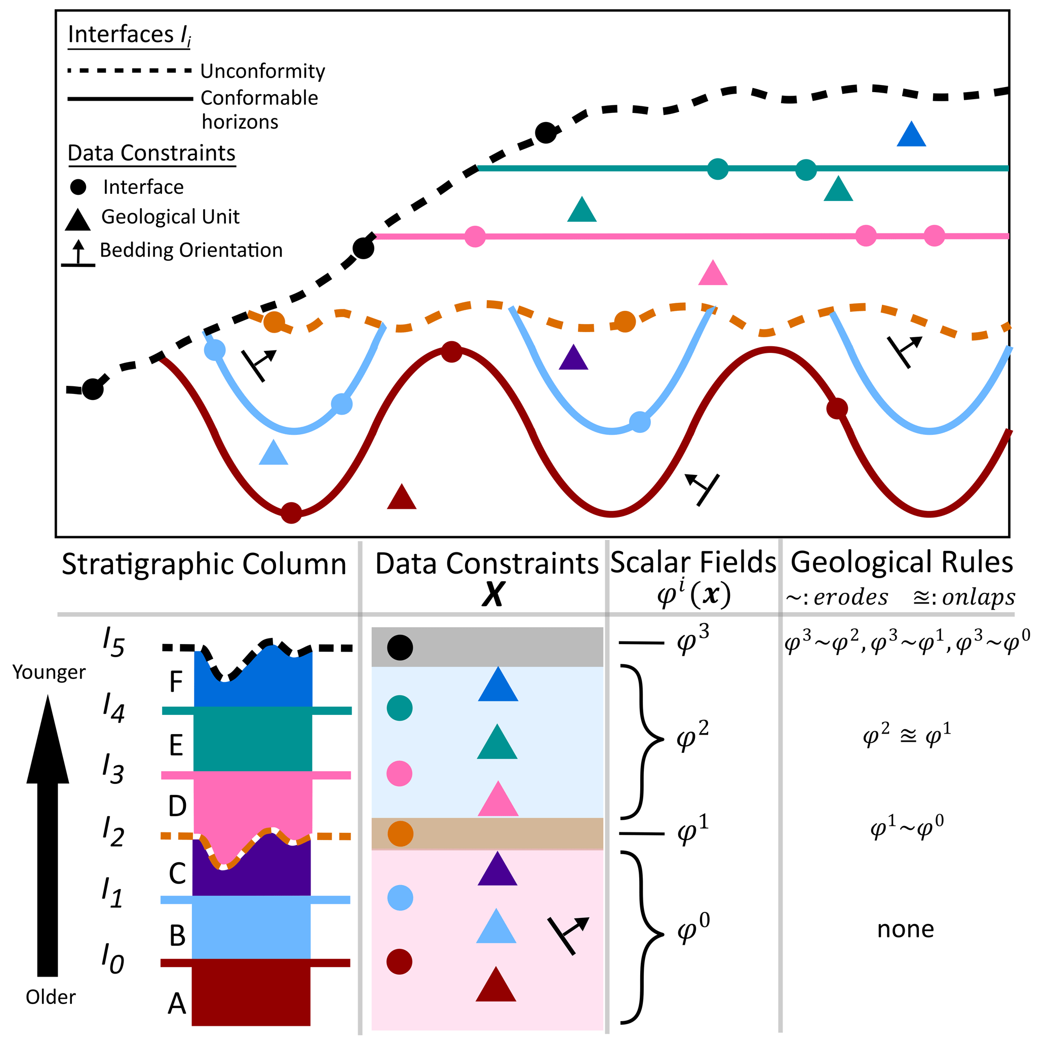
Figure 1 Complex geological setting for three-dimensional implicit geological modelling. Inputs for modelling include scattered data constraints, a stratigraphic column, and set of geological rules (erodes, ∼; onlaps, ≊) for scalar fields φⁱ(x) representing distinct conformal and unconformity structures.

Let $M\left(X,\mathit{\phi },\mathit{\xi }\right)$ be an implicit model in three-dimensional space where the point set $X=\left\{{\mathit{x}}_{\mathrm{0}},\mathrm{\dots },{\mathit{x}}_{N-\mathrm{1}}\right\}\subseteq {\mathbb{R}}^{\mathrm{3}}$ is the N scattered data points, the tuple $\mathit{\phi }=\left({\mathit{\phi }}^{\mathrm{0}},\mathrm{\dots },{\mathit{\phi }}^{F-\mathrm{1}}\right)$ is the F indexed implicit scalar fields, and ξ is a global smoothness constraint (Sect. 2.4.5). The global smoothness constraint is to ensure a globally reasonable geological structural model.

Let ${\mathit{\phi }}^i\left(X^i,I_k^i,U_k^i,O^i,\mathit{\epsilon }\right)$ be the ith implicit scalar field approximated from the set of points $X^i=\left\{X_{I_k^i},X_{U_k^i},X_{O^i}\right\}\subseteq X$ sampling interfaces $I_k^i$, geological units $U_k^i$, and orientations Oⁱ respectively. The scalar field is approximated from the set of interpolation constraints ε (Sect. 2.4) using these sampled data points. The set of interfaces $I_k^i$ and units $U_k^i$ are arranged in an order of older to younger.

2.3 Implicit neural representations

Implicit neural representations, also known as coordinate-based representations (Tancik et al., 2020), are neural networks that parameterize implicitly defined functions φ(x), where the network's inputs x∈ℝ^m are mth-dimensional spatial or spatial–temporal coordinates. These networks typically utilize a MLP, as illustrated in Fig. 2, to learn how to map coordinates into a geometrical representation of shape/structure encoded as an implicit scalar field. Note that other network architectures, such as GNNs (Hillier et al., 2021), that learn this mapping are also categorized as INR networks. MLPs are universal approximators capable of approximating any unknown function f(x) provided there are enough hidden neurons (Hornik et al., 1989). They are composed of three types of layers – input, hidden, and output layers – which transform inputted data into abstract representations and model predictions in the hidden and output layers, respectively. There are three parameters that define MLP networks: number of hidden layers N_h, dimensionality of representations d_rep, and chosen non-linear activation function σ. At every training iteration t, errors between the network's outputted scalar fields and interpolation constraints are measured using developed loss functions presented in the proceeding section. These errors are minimized by the backpropagation process where the network's variables (W's and b's Fig. 2a) are updated by gradient descent. For complex geologically settings where there are F distinct conformal and unconformity structures, each associated with a separate implicit scalar field φⁱ, F MLPs are stacked together, resulting in F scalar values being outputted for every point x (Fig. 2c). Following the training process, multiple scalar fields are combined in a manner respecting the geological rules for erosion and onlapping of conformal structures onto unconformities (Sect. 2.6).

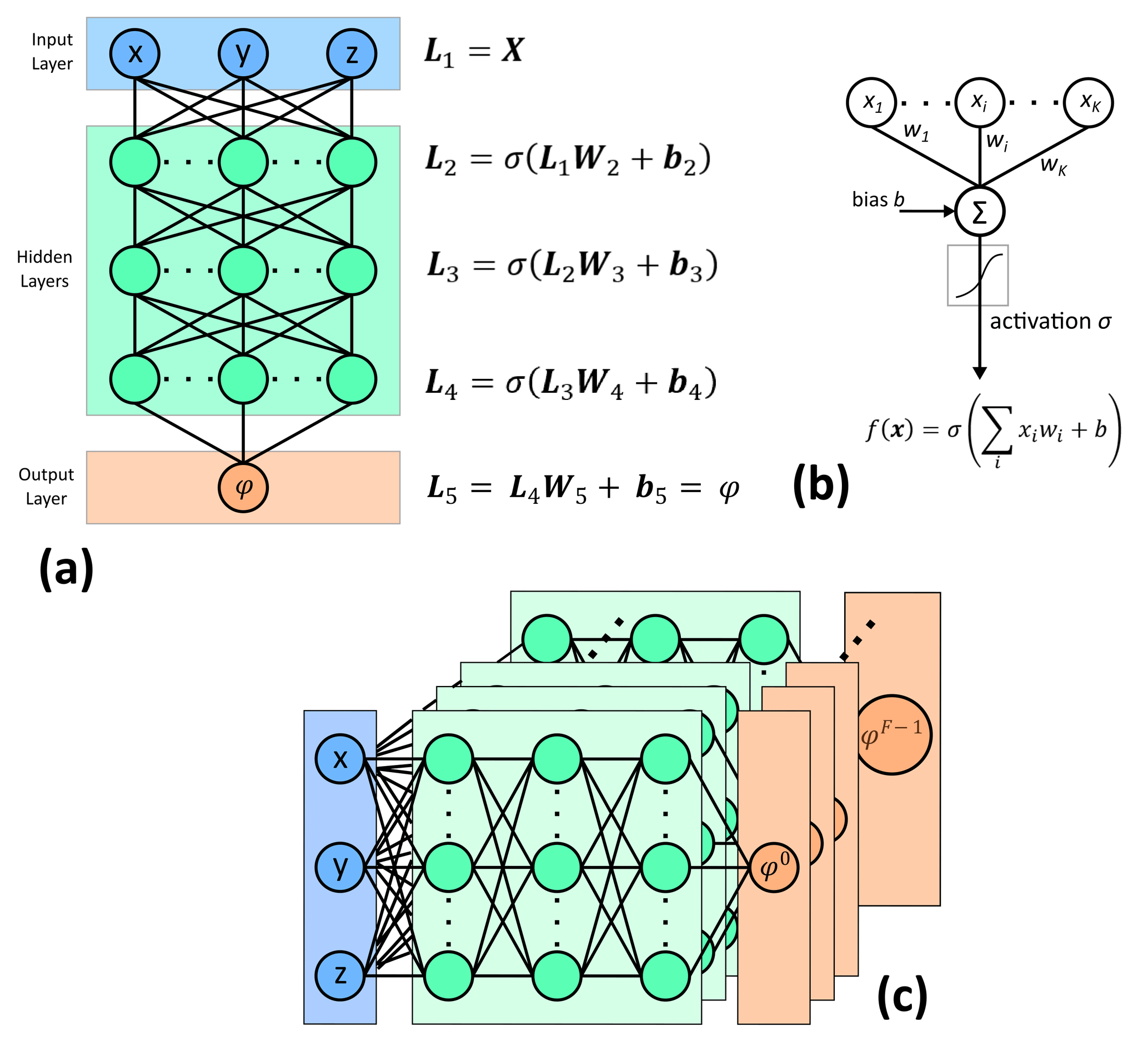
Figure 2 Neural network architecture for three-dimensional implicit geological modelling. (a) MLP architecture that generates scalar field predictions from spatial coordinates. (b) Perceptron neural model and output for a neuron. (c) Multiple scalar field predictions for a given point from stacked MLPs in the GeoINR network.

2.4 Interpolation constraints and loss functions

For structural geological modelling, interpolation constraints ε are split into four categories: interface, geological unit, orientation, and global smoothness constraints. For interface and geological unit data, a suite of knowledge constraints on stratigraphic relations are developed and described in the next section (Sect. 2.4.1). For each constraint type, a corresponding loss function is developed to accumulate all errors (Fig. 3), at every training iteration t, measured between the predicted model and set of points for which a constraint is imposed.

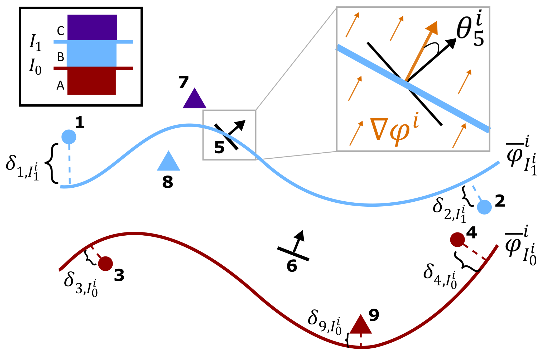
Figure 3 Errors associated with interface (circles), geological unit (triangles), and orientation (black arrows) constraints at training iteration t, modelling two conformal interfaces $I_{\mathrm{1}}^i$ and $I_{\mathrm{0}}^i$ and three geological units A, B, and C, with an implicit scalar field φⁱ. Approximated signed distances δ are computed for interface and geological unit data, whereas angular residuals θ are computed for orientation data. Insets: (black) stratigraphic column; (gray) angle between scalar gradient (orange) and bedding.

2.4.1 Stratigraphic relations and constraints

Stratigraphic relations are defined, in terms of scalar field differences, to encapsulate above, below, and on relationships (e.g., knowledge) between points sampling interfaces and geological units using a given stratigraphic column. From these relations, a suite of constraints for scattered point sets are developed so that the constrained implicit model M respects the stratigraphic column.

Given a point ${\mathit{x}}_l\in X_{{\mathrm{{\rm Y}}}_j}$ belonging to a point set $X_{{\mathrm{{\rm Y}}}_j}$ sampling either a specific interface (Υ_j=I_j) or geological unit (Υ_j=U_j), a stratigraphic relation is defined as follows:

$$\begin{array}{}\text{(2)}& R_{{\mathit{x}}_l,I_k^i}={\mathit{\phi }}_l^i-{\stackrel{\mathrm{‾}}{\mathit{\phi }}}_{I_k^i}^i,\end{array}$$

where ${\stackrel{\mathrm{‾}}{\mathit{\phi }}}_{I_k^i}^i$ (Eq. 1) is the iso-value, at training iteration t, associated with interface I_k and represented by scalar field φⁱ. The relation indicates whether point x_l is above, below, or on a reference interface I_k, modelled with scalar field φⁱ, when the relation value is

$$\begin{array}{}\text{(3)}& \begin{array}{rl}{R}_{{\mathit{x}}_l,I_k^i}>\mathrm{0}& \text{above},\\ R_{{\mathit{x}}_l,I_k^i}<\mathrm{0}& \text{below},\\ R_{{\mathit{x}}_l,I_k^i}=\mathrm{0}& \text{on},\end{array}\end{array}$$

respectively. Point sets $X_{{\mathrm{{\rm Y}}}_j}$ encoded as stratigraphically above or below an interface I_k are given the following inequality constraints:

$$\begin{array}{}\text{(4)}& \begin{array}{rl}& R_{{\mathrm{{\rm Y}}}_j,I_k^i}={\mathit{\phi }}_{{\mathrm{{\rm Y}}}_j}^i-{\stackrel{\mathrm{‾}}{\mathit{\phi }}}_{I_k^i}^i>\mathrm{0}\\ & R_{{\mathrm{{\rm Y}}}_j,I_k^i}={\mathit{\phi }}_{{\mathrm{{\rm Y}}}_j}^i-{\stackrel{\mathrm{‾}}{\mathit{\phi }}}_{I_k^i}^i<\mathrm{0},\end{array}\end{array}$$

respectively. For a point set sampling the reference interface I_k, the constraint

$$\begin{array}{}\text{(5)}& R_{I_k,I_k^i}={\mathit{\phi }}_{I_k}^i-{\stackrel{\mathrm{‾}}{\mathit{\phi }}}_{I_k^i}^i=\mathrm{0}\end{array}$$

is used. The complete set of stratigraphic constraints on relations for both interface and geological unit point data illustrated in Fig. 1 is shown in Fig. 4. The set of relations considers interface–interface and unit–interface pairs, and they are expressed in matrix form with above relations (yellow) in the upper right and below relations (light purple) in the lower left. For the matrix of interface–interface relations, on relations (green) are along the diagonal. For the above relations and associated constraints, only the ones within distinct geological domains – created by the series of unconformity interfaces – are considered, while the remaining ones (red) are discarded. These are discarded because points sampling younger geological features can be measured as being below older modelled interfaces from other geological domains using their associated scalar fields and corresponding iso-value, depending on their geometries. For example, consider the unconformity interface I₂ (Fig. 4), it erodes portions of I₁ and therefore the presence of the unconformity can be measured below I₁ using φ⁰ (e.g., the scalar field that models I₁) in those portions. This characteristic does not apply to any below relations and constraints, since points sampling an interface or unit must always be below all younger interfaces. In our available source code, we also provide a more efficient alternative option for below relations: excluding below relations of conformal interfaces and associated units with younger conformal interfaces from younger geological domains. Only below relations of conformal interfaces and associated units to the next youngest unconformity are required to constrain their geometries.

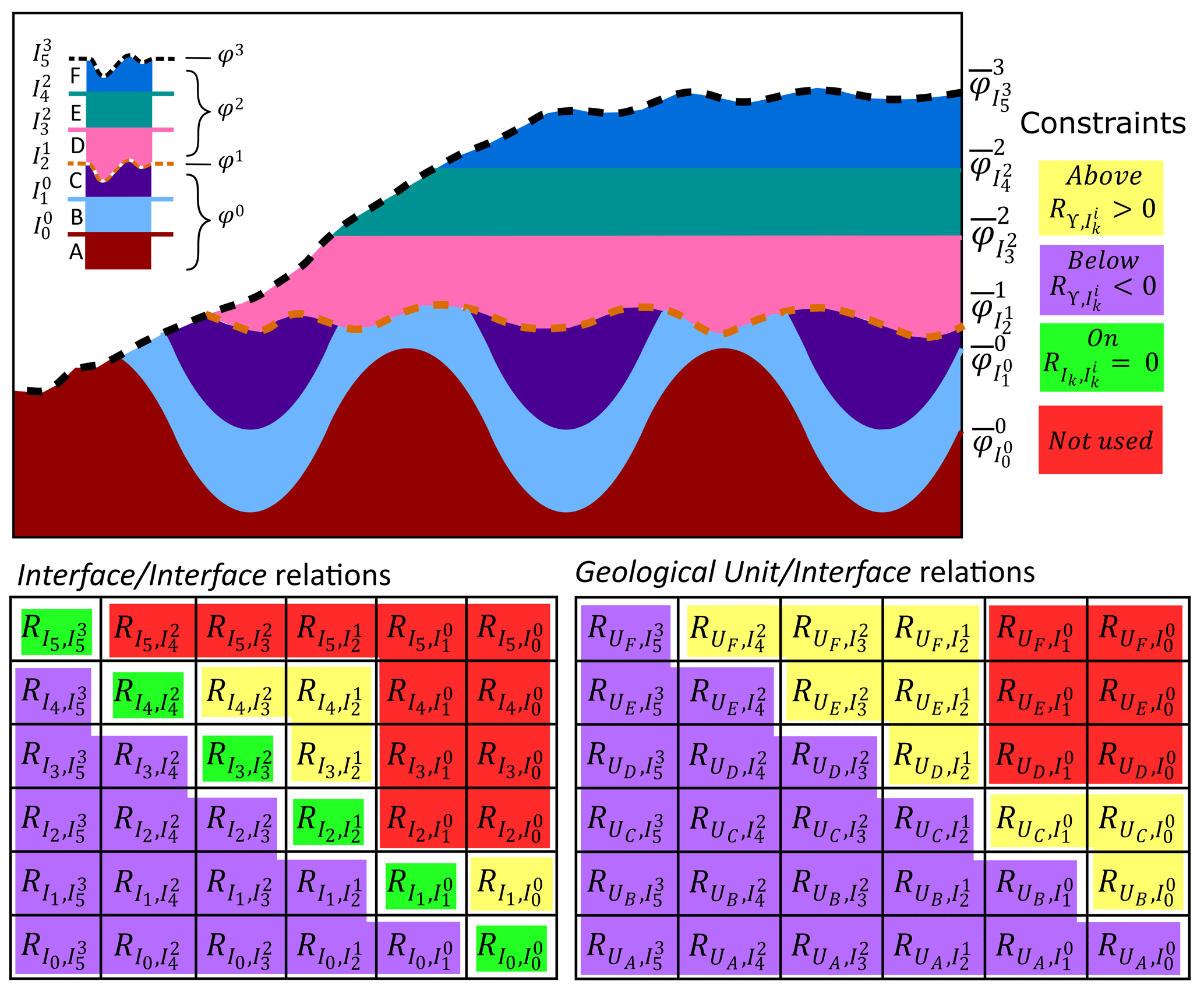
Figure 4 Stratigraphic relations between specific interface–interface and geological unit–interface pairs and associated constraints. Constraints are colored according to their above (yellow), below (light purple), or on (green) spatial relation. For above relations (upper right matrix block), only the constraints on relations within distinct geological domains are considered, while the remaining constraints are not used (red).

To measure errors at some training iteration t between the implicit model M at sampled interfaces and geological unit points x_l and their associated constraints, approximate signed distances ${\mathit{\delta }}_{{\mathit{x}}_l,I_k^i}$ (Caumon, 2010; Taubin, 1994) (Fig. 3) from a reference interface I_k, modelled by φⁱ, are used and defined as follows:

$$\begin{array}{}\text{(6)}& {\mathit{\delta }}_{{\mathit{x}}_l,I_k^i}={\displaystyle \frac{{\mathit{\phi }}_l^i-{\stackrel{\mathrm{‾}}{\mathit{\phi }}}_{I_k^i}^i}{∥\mathrm{\nabla }{\mathit{\phi }}_l^i∥}}.\end{array}$$

The magnitude of the scalar gradient $∥\mathrm{\nabla }{\mathit{\phi }}_l^i∥$ in the denominator is an important term to account for changes in unit thickness between interfaces represented by the scalar field. Smaller magnitudes correspond to thickening of units, while larger ones are indicative of unit thinning. Consequently, the approximate signed distances are a much more accurate measure of how far above or below a point is above some reference interface than the scalar differences themselves. This is because scalar values for various geological features are not meaningful in real-world distances and are not normalized between features.

The three loss functions for the above, below, and on stratigraphic constraints integrating all errors from point sets X_Υ are given by

$$\begin{array}{}\text{(7)}& {\displaystyle }\begin{array}{rl}{L}_{\mathrm{{\rm Y}}}^{\mathrm{Above}}& =\sum _{{\mathrm{{\rm Y}}}_j\in \mathrm{{\rm Y}}}^{\left|\mathrm{{\rm Y}}\right|}{\displaystyle \frac{\mathrm{1}}{\left|X_{{\mathrm{{\rm Y}}}_j}\right|}}\sum _{{\mathit{x}}_l\in X_{{\mathrm{{\rm Y}}}_j}}^{\left|X_{{\mathrm{{\rm Y}}}_j}\right|}\sum _{I_k^i\in B_{{\mathrm{{\rm Y}}}_j}}^{\left|B_{{\mathrm{{\rm Y}}}_j}\right|}{\widehat{\mathit{\delta }}}_{{\mathit{x}}_l,I_k^i},\\ & {\widehat{\mathit{\delta }}}_{{\mathit{x}}_l,I_k^i}=\left\{\begin{array}{c}\begin{array}{cc}\frac{\left|{\mathit{\phi }}_l^i-{\stackrel{\mathrm{‾}}{\mathit{\phi }}}_{I_k^i}^i\right|}{∥\mathrm{\nabla }{\mathit{\phi }}_l^i∥}& {\mathit{\phi }}_l^i-{\stackrel{\mathrm{‾}}{\mathit{\phi }}}_{I_k^i}^i<\mathrm{0}\end{array}\\ \begin{array}{cc}\mathrm{0}& {\mathit{\phi }}_l^i-{\stackrel{\mathrm{‾}}{\mathit{\phi }}}_{I_k^i}^i\end{array}\ge \mathrm{0}\end{array}\right.\end{array}\text{(8)}& {\displaystyle }\begin{array}{rl}{L}_{\mathrm{{\rm Y}}}^{\mathrm{Below}}& =\sum _{{\mathrm{{\rm Y}}}_j\in \mathrm{{\rm Y}}}^{\left|\mathrm{{\rm Y}}\right|}{\displaystyle \frac{\mathrm{1}}{\left|X_{{\mathrm{{\rm Y}}}_j}\right|}}\sum _{{\mathit{x}}_l\in X_{{\mathrm{{\rm Y}}}_j}}^{\left|X_{{\mathrm{{\rm Y}}}_j}\right|}\sum _{I_k^i\in A_{{\mathrm{{\rm Y}}}_j}}^{\left|A_{{\mathrm{{\rm Y}}}_j}\right|}{\stackrel{\mathrm{ˇ}}{\mathit{\delta }}}_{{\mathit{x}}_l,I_k^i},\\ & {\stackrel{\mathrm{ˇ}}{\mathit{\delta }}}_{{\mathit{x}}_l,I_k^i}=\left\{\begin{array}{c}\begin{array}{cc}\frac{{\mathit{\phi }}_l^i-{\stackrel{\mathrm{‾}}{\mathit{\phi }}}_{I_k^i}^i}{∥\mathrm{\nabla }{\mathit{\phi }}_l^i∥}& {\mathit{\phi }}_l^i-{\stackrel{\mathrm{‾}}{\mathit{\phi }}}_{I_k^i}^i>\mathrm{0}\end{array}\\ \begin{array}{cc}\mathrm{0}& {\mathit{\phi }}_l^i-{\stackrel{\mathrm{‾}}{\mathit{\phi }}}_{I_k^i}^i\end{array}\le \mathrm{0}\end{array}\right.\end{array}\text{(9)}& {\displaystyle }{L}_I^{\mathrm{On}}=\sum _k^{\left|I\right|}{\displaystyle \frac{\mathrm{1}}{\left|X_{I_k}\right|}}\sum _{{\mathit{x}}_l\in X_{I_k}}^{\left|X_{I_k}\right|}\left|{\mathit{\delta }}_{{\mathit{x}}_l,I_k^i}\right|\end{array}$$

respectively. Note that $A_{{\mathrm{{\rm Y}}}_j}$ and $B_{{\mathrm{{\rm Y}}}_j}$ are a set of interfaces $I_k^i$ that are above or below, respectively, a specific geological feature Υ_j (either an interface or unit). For example, consider the loss function for the below constraints (Eq. 8) associated with the geological unit U_D from Fig. 4. In this case, Υ_j=U_D and $A_{{\mathrm{{\rm Y}}}_j}=A_{U_D}=\left\{I_{\mathrm{5}}^{\mathrm{3}},I_{\mathrm{4}}^{\mathrm{2}},I_{\mathrm{3}}^{\mathrm{2}}\right\}$ are the set of interfaces above that geological unit. The below constraints for this geological unit require that the points within the set $X_{U_D}$ must be below the interfaces above $A_{U_D}$. If points ${\mathit{x}}_l\in X_{U_D}$ are above, or ${\mathit{\phi }}_l^i-{\stackrel{\mathrm{‾}}{\mathit{\phi }}}_{I_k^i}^i>\mathrm{0}$, those points will have non-zero errors; otherwise the error will be zero (e.g., constraint respected).

Loss functions associated with above or below stratigraphic constraints are effective in constraining resultant implicit models to respect the sequence provided by a given stratigraphic column. These loss functions ensure not only that modelled interfaces and strata respect the stratigraphic sequence for each scalar field φⁱ but also importantly that they respect the presence of sampled interfaces and strata associated with other scalar fields. To clearly illustrate the latter, consider Fig. 5 where two unconformities are modelled separately with two scalar fields. Without these constraints, unconformities are modelled independently, and a portion of the older unconformity is eroded incorrectly despite the presence of a valid unconformity observation point (e.g., point 1, Fig. 5a). With these constraints, all scalar fields are coupled so that the entire geological sequence of all sample interfaces and strata are honored/considered. This resolves an issue in other implicit approaches (Calcagno et al., 2008; de la Varga et al., 2019; Grose et al., 2021b) that treat each scalar field independently. And finally, these constraints help impose the correct scalar field polarity – e.g., the alignment of the gradient of the scalar field ∇φ with younging direction (direction of younger stratigraphy) – even in circumstances where there are no bedding observations available. Having the correct scalar field polarity is critical in assigning geological domains so that multiple scalar fields can be combined into a resultant scalar field respecting geological rules (erosional and onlap), as well as assigning geological units to modelled volumes (Sect. 2.6).

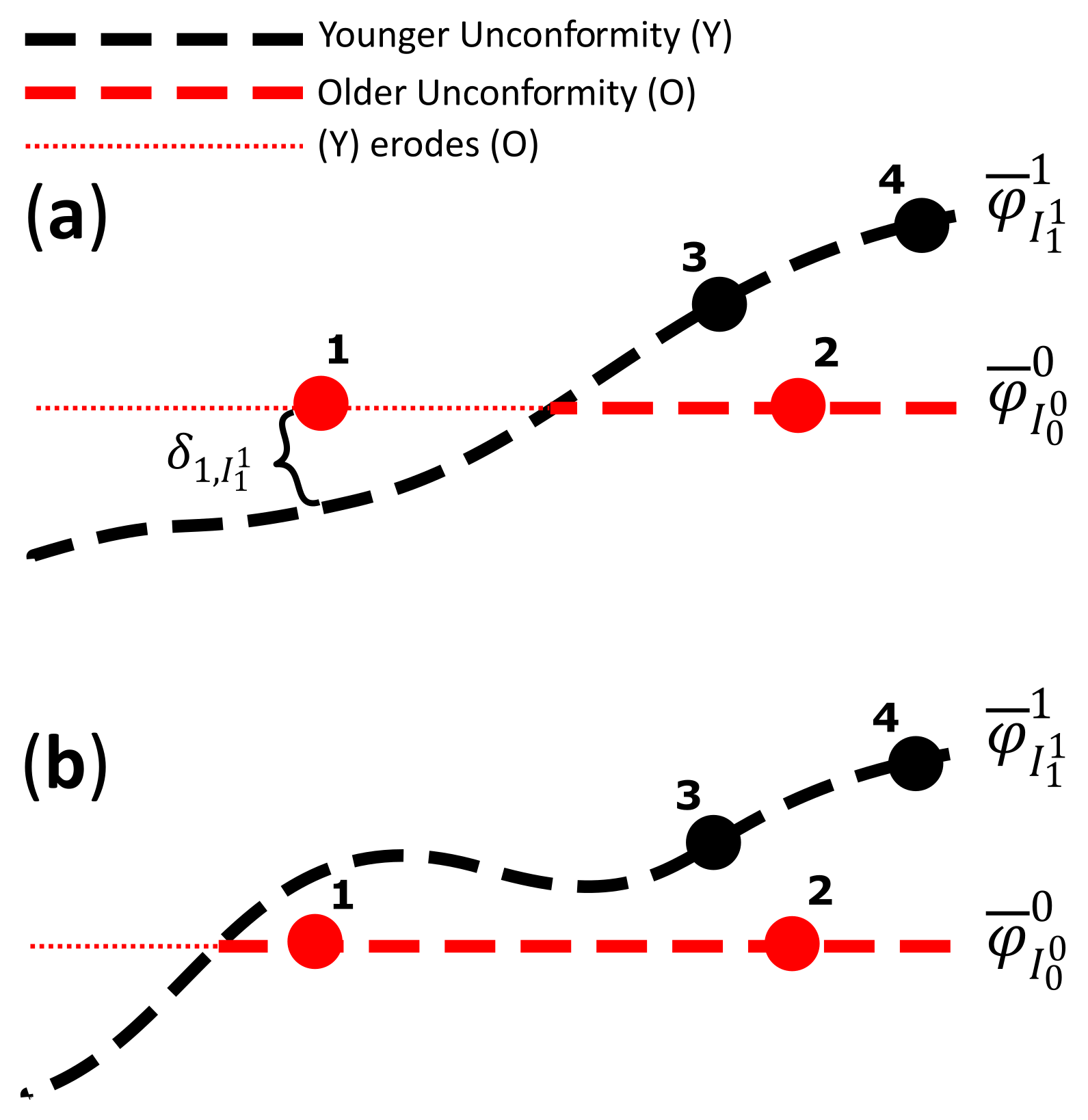
Figure 5 The effect of above and below stratigraphic constraints in coupling two scalar fields φ⁰ and φ¹ modelling two unconformities. (a) Without using the constraints and (b) with using the constraints.

2.4.2 Interface constraints

For interface data, there are four interpolation constraints. Firstly, the variance of all scalar field values ${\mathit{\phi }}_{I_k^i}^i$ on a sampled interface $I_k^i$ is roughly zero as follows:

$$\begin{array}{}\text{(10)}& \mathrm{Var}\left({\mathit{\phi }}_{I_k^i}^i\right)=\mathrm{0}.\end{array}$$

This iso-value constraint ensures that the scalar field at the sampled locations for kth interface $X_{I_k}$ is the same and has the following associated loss function:

$$\begin{array}{}\text{(11)}& L_I^{\mathrm{var}}=\sum _{I_k\in I}^{\left|I\right|}\mathrm{Var}\left({\mathit{\phi }}_{I_k^i}^i\right).\end{array}$$

The other three constraints utilize the stratigraphic relations to enforce the above, below, and on constraints. Combined, the resulting loss function for interface data is as follows:

$$\begin{array}{}\text{(12)}& L_I=L_I^{\mathrm{var}}+L_I^{\mathrm{On}}+L_I^{\mathrm{Above}}+L_I^{\mathrm{Below}}.\end{array}$$

The first two loss functions both constrain the implicit model to respect the locations of sampled interfaces, while the last two ensure that the sequence of sampled interfaces respects the given stratigraphic column.

2.4.3 Geological unit constraints

To constrain the implicit model with geological unit data U, the above and below stratigraphic constraints are applied. Consequently, the resulting loss function for geological unit data is as follows:

$$\begin{array}{}\text{(13)}& L_U=L_U^{\mathrm{Above}}+L_U^{\mathrm{Below}}.\end{array}$$

2.4.4 Orientation constraints

For an orientation data point ${\mathit{x}}_j\in X_{O^i}$ associated with a scalar field φⁱ, an angular constraint ${\mathit{\theta }}_j^{\mathrm{C}}$ characterizes the angle between the orientation vector v_j and the scalar gradient $\mathrm{\nabla }{\mathit{\phi }}_j^i$ at x_j. For normal data (e.g., bedding orientation with younging direction), the interpolation constraint is

$$\begin{array}{}\text{(14)}& {\mathit{\theta }}^{\mathrm{C}}=\mathrm{0}{}^{\circ },\end{array}$$

while for tangent data (e.g., lineations, fold axis) it is

$$\begin{array}{}\text{(15)}& {\mathit{\theta }}^{\mathrm{C}}=\mathrm{90}{}^{\circ }.\end{array}$$

The loss function associated with orientation data θⁱ measures angular errors (Fig. 3) between the given angular constraints ${\mathit{\theta }}_j^{\mathrm{C}}$ and angles ${\mathit{\theta }}_j^i$ computed from the implicit model M at some training iteration, and it is given by

$$\begin{array}{}\text{(16)}& L_O=\sum _{i=\mathrm{1}}^F{\displaystyle \frac{\mathrm{1}}{\left|O^i\right|}}\sum _{j\in O^i}^{\left|O^i\right|}\left|\cos {\mathit{\theta }}_j^{\mathrm{C}}-\cos {\mathit{\theta }}_j^i\right|,\end{array}$$

where $\cos {\mathit{\theta }}_j^i$ is computed from

$$\begin{array}{}\text{(17)}& \cos {\mathit{\theta }}_j^i={\displaystyle \frac{{\mathit{v}}_j\cdot \mathrm{\nabla }{\mathit{\phi }}_j^i}{∥{\mathit{v}}_j∥∥\mathrm{\nabla }{\mathit{\phi }}_j^i∥}}.\end{array}$$

2.4.5 Global smoothness constraint

It is well established that a disadvantage of implicit approaches for structural geological modelling is that they can produce modelling artifacts, commonly referred to as “bubbly” artifacts, yielding geologically unreasonable models particularly in complex structural settings (de Kemp et al., 2017). One way to address this problem is to impose a global smoothness constraint over the modelling domain using energy minimization principles. Here, we use the eikonal constraint (e.g., a unit-norm constraint) (Gropp et al., 2020)

$$\begin{array}{}\text{(18)}& ∥\mathrm{\nabla }{\mathit{\phi }}^i\left(\mathit{x}\right)∥=\mathrm{1}\end{array}$$

for this purpose. The associated loss function for the implicit model is as follows:

$$\begin{array}{}\text{(19)}& L_{\mathit{\xi }}=\sum _i^F{\displaystyle \frac{\mathrm{1}}{\left|{\mathrm{\Omega }}_{\mathrm{s}}\right|}}\sum _{{\mathit{x}}_j\in {\mathrm{\Omega }}_{\mathrm{s}}}^{\left|{\mathrm{\Omega }}_{\mathrm{s}}\right|}\left(\left|∥\mathrm{\nabla }{\mathit{\phi }}_j^i∥-\mathrm{1}\right|\right),\end{array}$$

where Ω_s represents a set of points sampling the modelling domain Ω. Due to the efficiency and computational scalability of MLP neural networks, sufficiently sampling the domain, even densely, is feasible. The effect of the global smoothness constraint on the scalar field is that it promotes sub-parallel geometries in nearby strata throughout a modelling domain. The effect is illustrated in the first case study (Sect. 3.1).

2.4.6 Resultant loss function

The resultant loss function, or total loss function L, for all geological constraints is simply the sum of the individual loss functions and is given by

$$\begin{array}{}\text{(20)}& L=L_I+L_U+L_O+\mathit{\lambda }{L}_{\mathit{\xi }},\end{array}$$

where the loss function L_ξ for the global smoothness constraint is weighted by the lambda term, λ≥0. The larger its value, the more scalar fields are smoothed. This function represents the loss landscape (Li et al., 2018), or objective function, given a set of constraints and in which the learning algorithm attempts to find its minimum. The location in which the loss landscape is a minimum corresponds to the set of neural network variables that yield minimal error between the network's predictions and geological constraints.

2.5 Training

An important training aspect to our proposed INR networks is the geometrical initialization of network variables. The variables are initialized such that the resulting outputted scalar field represents a shape with reasonable starting geometry for a specific geological application, which will be evolved through training by fitting given data constraints. Using standard variable random initialization schemes (Glorot and Bengio, 2010; He et al., 2015), resulting output scalar fields can be far from an optimal starting point for training, especially as the network's complexity increases (Fig. 6a). Consequently, if the training algorithm is rerun many times using the same conditions (Fig. 6b), resulting structural models can exhibit large variance in modelled structures. To solve these issues, training starts with a geometrically reasonable scalar field by geometrical initialization of network variables. For intrusive-like modelling, network variables are initialized to produce a spherical geometry (Fig. 6c) (Atzmon and Lipman, 2020), whereas for stratigraphic modelling, they are initialized to produce a planar geometry (Fig. 6d).

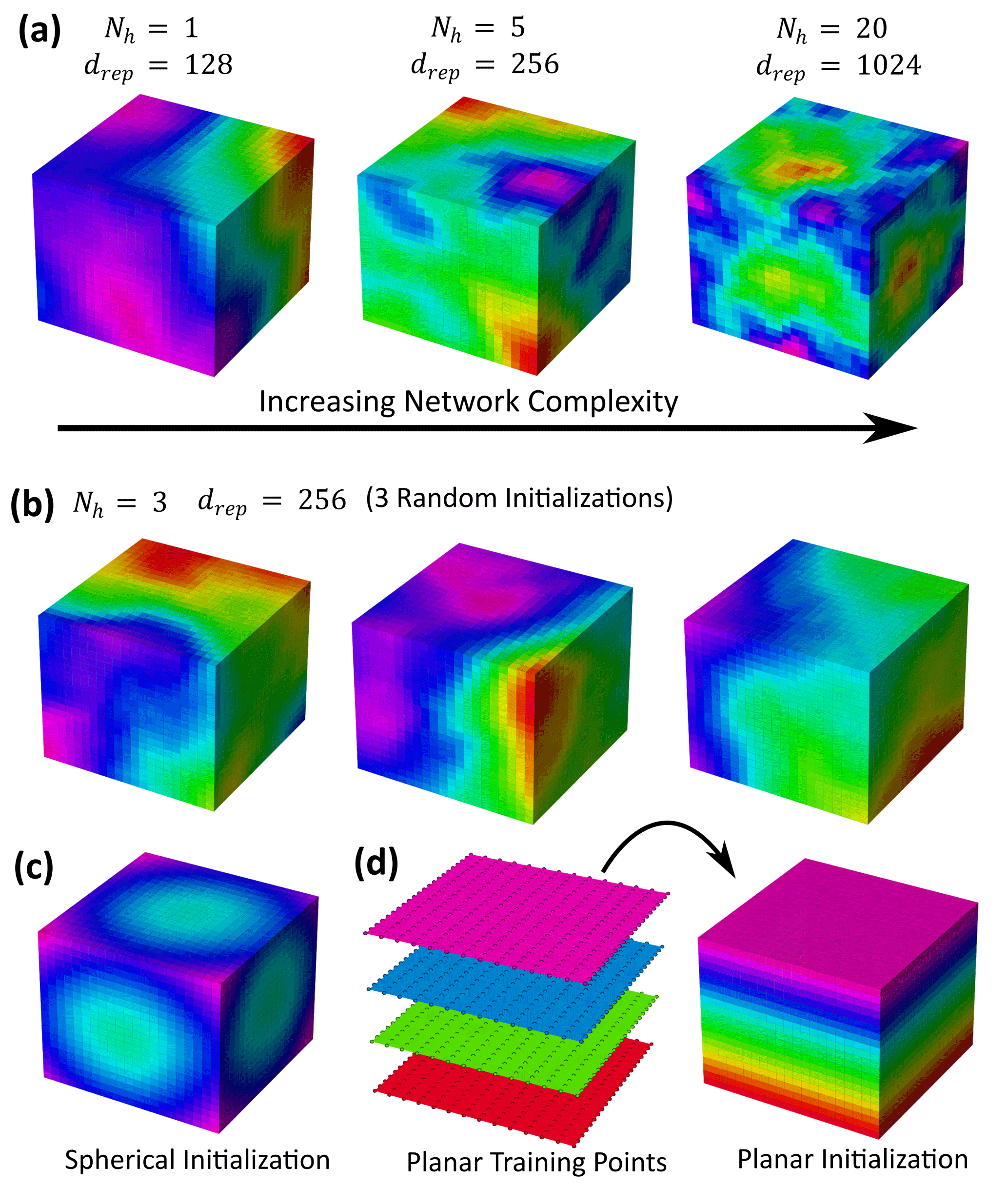
Figure 6 Scalar fields generated from initialization of network variables. (a) Effect of increasing network complexity on the generated scalar field by increasing the number of hidden layers N_h and dimension of hidden representations d_rep. (b) Scalar fields generated from three random initializations of network variables. (c) Spherical initialization. (d) Planar initialization using a pre-trained network applied to points sampling layer–cake volume.

To initialize our networks to produce a scalar field with a planar geometry, we first pre-train a MLP network for 1000 epochs with the same parameterization (N_h, d_rep, σ) on a synthetic dataset densely sampling four layer–cake interfaces (Fig. 6d). The pre-trained network's parameters are saved and loaded into each of the F stacked MLP networks, which are updated by training on an unseen stratigraphic dataset. This can be viewed as transfer learning (Zhuang et al., 2021): applying what is learned for one problem onto a similar problem. An added benefit to using pre-trained networks is reproducibility in modelling results since the network is initialized with the same parameters. Furthermore, the number of training epochs to converge is reduced.

Another training aspect utilized in the proposed methodology is applying learning rate schedules in the Adam optimizer (Loshchilov and Hutter, 2017). Learning rate schedules adjust the learning rate during training by decreasing the rate according to a prescribed schedule. While the Adam optimizer does adapt the initialized learning rate on a per-parameter basis, there is a benefit to decreasing the adaptable learning rate with increasing training epochs. Empirically, we have found that applying either step decay or cosine annealing learning rate schedules yields much lower losses and consequently better data fitting characteristics.

2.6 Geological domains and combining scalar field series

After implicit scalar functions are constrained by training, gridded points sampling a geological volume are inputted to the trained MLP network to generate F separate continuous scalar fields, each representing a distinct geological feature, throughout the volume of interest (Fig. 7a). Since unconformity interfaces can erode (e.g., cut) older geological features, there are regions of space where those features are no longer present. To cut portions of a geological feature removed by an unconformity, its associated continuous scalar field is cut by the modelled unconformity interface. As a result, geological features are partitioned into geological domains (Fig. 7b) where those features are present, and their associated scalar fields and geological units are defined (Fig. 7c). Since a point in the modelled volume can only be associated with a single scalar field, the scalar field series and their associated geological units are combined such that only the domain in which each scalar field and set of units is defined is merged into a resultant scalar field and geological unit model (Fig. 7d).

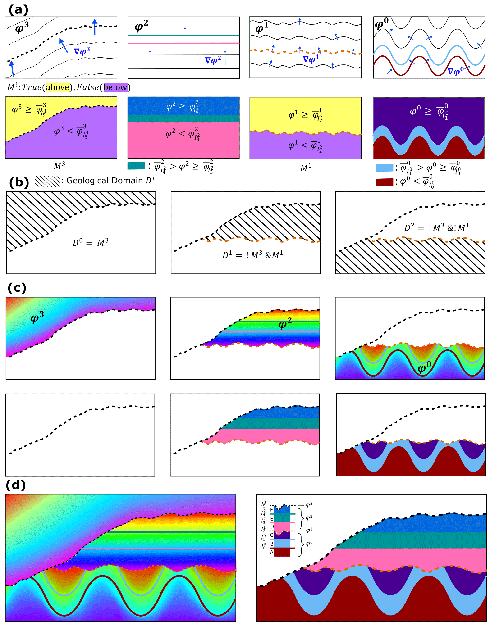
Figure 7 Constructing geological domains and combining scalar fields. (a) (top) Scalar field series and modelled interfaces with their regions (bottom) defined from associated inequalities. Scalar fields associated with unconformities have Boolean masks Mⁱ defining above and below regions. (b) Geological domains constructed from Boolean masks. (c) Scalar fields and geological units assigned to geological domains. (d) Combined scalar fields and geological units.

Geological domains are spatial partitions created by boundaries defining discontinuous features (e.g., unconformities) within which continuous geological features (e.g., conformable stratigraphy) exist. In this paper, only unconformity boundaries are used to create geological domains, although the same approach can be used for faulting. See discussion (Sect. 4) for future work with incorporation of faulting. To construct geological domains, first mask arrays defining above and below (Fig. 7b) regions for each unconformity interface within the modelling volume are computed using the associated scalar field and inequalities. As mentioned previously, the notion of above/below a reference interface defined by an iso-value, also known as polarity, is provided by the scalar gradient (Fig. 7a) that points in the direction of younger stratigraphy (e.g., younging direction). For example, volumes above and below an interface I₅ modelled with φ³ are defined, respectively, by

$$\begin{array}{}\text{(21)}& \begin{array}{rl}& {\mathit{\phi }}^{\mathrm{3}}\ge {\stackrel{\mathrm{‾}}{\mathit{\phi }}}_{I_{\mathrm{5}}^{\mathrm{3}}}^{\mathrm{3}}\\ & {\mathit{\phi }}^{\mathrm{3}}<{\stackrel{\mathrm{‾}}{\mathit{\phi }}}_{I_{\mathrm{5}}^{\mathrm{3}}}^{\mathrm{3}},\end{array}\end{array}$$

where ${\stackrel{\mathrm{‾}}{\mathit{\phi }}}_{I_{\mathrm{5}}^{\mathrm{3}}}^{\mathrm{3}}$ is the iso-value associated with I₅. The mask array Mⁱ associated with the unconformity is set to true wherever above the interface and false below it. Secondly, from the geological rules associated with the unconformity scalar fields, an appropriate set of Boolean logic is applied to the mask array(s) to define the geological domain. For example, consider domain D¹ in Fig. 7b; it is defined wherever it is below I₅ (where M³ is false; !M³) and above I₂ (where M¹ is true; M¹). Domains for older geological features have a larger set of Boolean logic applied to mask arrays since there are more younger unconformities that can erode those volumes as compared to younger geological features. With the geological domains defined, scalar fields and geological units are both assigned to their associated geological domains, thereby combining all the scalar fields and geological units into a resultant three-dimensional geological volumetric model.

2.7 Iso-surface extraction

Iso-surface extraction methods can be applied to specific regions of implicit scalar field volumes provided appropriate Boolean masks are given and can be useful for obtaining the geological horizons of conformal domains. However, obtaining unconformity interfaces using this approach will lead to the production of anti-aliasing artifacts in triangulated surfaces. To resolve this issue, we develop an algorithm (see Algorithm 1 in Appendix A) using the open-source library PyVista (Sullivan and Kaszynski, 2019) to generate all iso-surfaces that can be cut by unconformities. The algorithm first extracts the set of continuous iso-surfaces for each of the F scalar fields computed within a gridded volume. Next, the set of iso-surfaces are iterated on, going from oldest to youngest and processed. For a given surface being processed, that surface is progressively cut by younger unconformities above it in the stratigraphic column, again going from older to younger.

3 Case studies

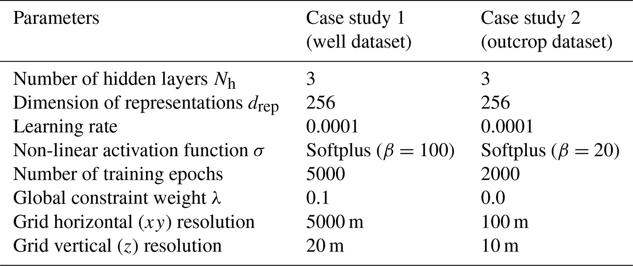
Modelling results are presented for two real-world case studies to demonstrate proof of concept: (1) a sedimentary basin with large, dense, and noisy well data and (2) a deformed metamorphic setting with sparse outcrop data. For both case studies, the learnable variables of our network, called GeoINR, are initialized with pre-trained models with planar geometry (described in Sect. 2.5) using the model parameters summarized in Table 1. These variables are updated using the Adam optimizer within the PyTorch framework so that modelling errors are minimized during training through the backpropagation process. Moreover, the cosine annealing learning rate scheduler was used with this optimizer. The network architecture parameters ($N_{\mathrm{h}},d_{\mathrm{rep}},\mathit{\sigma }$) and learning rate were established from INR literature (Atzmon and Lipman, 2020; Gropp et al., 2020; Park et al., 2019; Sitzmann et al., 2020; Tancik et al., 2020) and refined through trial and error using various combinations of parameter values. The non-linear activation function used for our networks was the parameterized Softplus function:

$$\begin{array}{}\text{(22)}& \mathit{\sigma }\left(x\right)={\displaystyle \frac{\mathrm{1}}{\mathit{\beta }}}\log \left(\mathrm{1}+e^{\mathit{\beta }x}\right),\end{array}$$

where the parameter β controls the variability of modelled interfaces. Smaller values of β produce flatter modelled interfaces, whereas higher values produce more locally variant modelled interfaces. For these case studies and other synthetic structural geological models, these parameters produce structurally consistent models with respect to the sampled point constraints.

Table 1 GeoINR model parameters values for case studies.

Organizing geological point datasets first requires all necessary knowledge to be extracted from a stratigraphic column. Stratigraphic knowledge including the geological rule of the interface (e.g., erosional, or onlap (conformable)) and the set of interfaces above and below each interface and geological unit are tabulated (see Appendix B for tables associated with both case studies). Corresponding tables describe the set of stratigraphic relations (Sect. 2.4.1) and associate interfaces and units to a particular scalar field among the series. This information is used for implementation purposes so that associated loss functions can compute measuring errors between the stratigraphic constraints and the version of the model at some training iteration t.

As with any machine-learning algorithm, neural network inputs require normalization for the network to learn useful latent representations and yield accurate predictions. Inputs for INR networks, which are spatial coordinates in this case, are normalized to some range for each coordinate dimension. For the first case study, each coordinate dimension is normalized to the [−1, 1] range. This is particularly important for the first case study where the dataset is covering a large geographical area. Having a constant scaling term for each coordinate dimension for this case study is not possible because there would be negligible variation in z coordinates; network's losses do not decrease with training. In addition, it is worth noting that if orientation data are available for datasets covering large geographical areas (> 1000 km), scalar field gradients computed from the network are required to be transformed back into the original space – using the associated scaling term for each coordinate dimension. This is required to accurately measure the angular residuals to constrain orientational data. For the second case study, each coordinate dimension has the dataset's center subtracted then scaled by the maximum range of $\mathrm{\Delta }x,\mathrm{\Delta }y,\mathrm{\Delta }z$ (Hillier et al., 2021) since there is sufficient variation in normalized z coordinates due to the much smaller geographical extents.

After the networks are trained using the supplied data and knowledge constraints, inference is performed on all the points within a voxel grid (e.g., grid corners) covering the volume of interest. At these points, predicted scalar field values and geological units are computed. Once computed, scalar fields and geological units are assigned to geological domains, followed by iso-surface extraction of modelled interfaces.

Results for both case studies were obtained using a high-end desktop PC with an Intel Core i9-9980XE CPU and a single NVIDIA RTX 2080 Ti GPU.

3.1 Provincial-scale sedimentary basin case study

The first case study is of a provincial-scale sedimentary basin covering an area approximately 451 000 km² using a well dataset of formation tops and unconformity picks from the Lower Paleozoic portion of the Western Canadian Sedimentary Basin (WCSB) in Saskatchewan, Canada (extracted from March and Love, 2014). The interface constraint data consist of 4708 formation tops and unconformity picks sampling four unconformities and three conformable horizons. The depths of the picks were interpreted from geophysical well logs and correlated to core samples when available. Due to the interpretative nature of the constraint data, it can be characterized as noisy as their exact positions are uncertain (Fig. 8a (right)). But this presents an opportunity to test whether the proposed methodology is useful for modelling data commonly obtained by Geological Survey Organizations (GSO). In addition to interface constraint data, augmented data consisting of intraformational units were generated by sampling along well intervals to demonstrate their modelling impact. These augmented data are not required to produce a geologically representative model (Fig. 8b) but serve to demonstrate that the methodology successfully handles this type of data. Intraformational units are sampled along a well interval between two interfaces only if the interfaces are stratigraphically adjacent. Interpreted depths of successive formation tops (e.g., interfaces) along the well path may not always be stratigraphically adjacent, either because the top could not be identified or a portion of stratigraphy was eroded. In these cases, intraformational units are not sampled along a well interval (Fig. 9). For this case study, sequenced well intervals were sampled at every 20 m (vertical resolution of our voxel grid; 5 km was the horizontal resolution) and generated 11 270 sampled intraformational units. Two three-dimensional implicit geological models are produced: one using both interface and intraformational points and the other having just interface points.

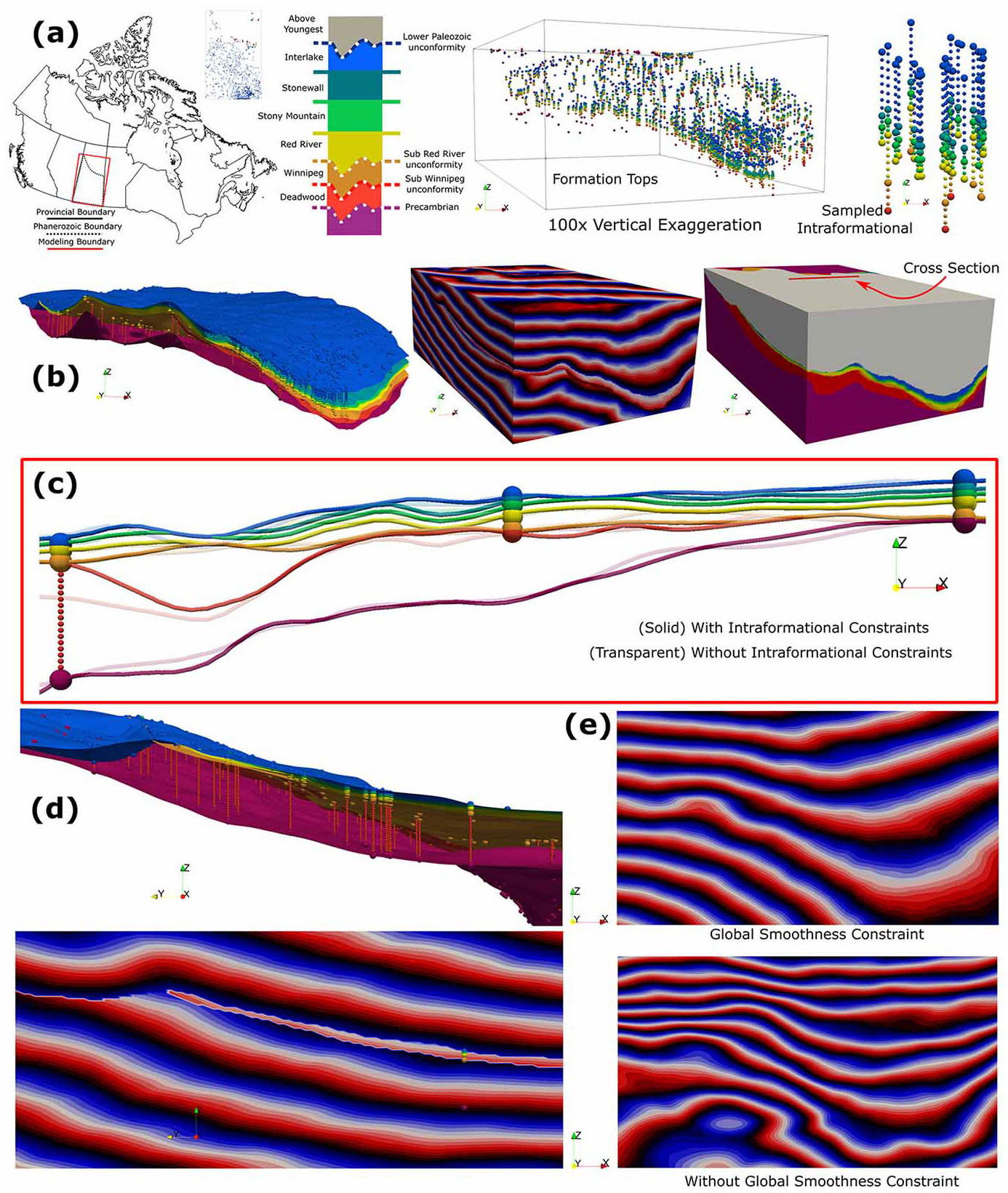
Figure 8 Modelling results for the Lower Paleozoic portion of the WCSB in Saskatchewan generated using the proposed GeoINR methodology. Data and modelled results use 100× vertical exaggeration to visualize the provincial-scale model. (a) Model's geographical coverage, stratigraphic column, formation tops (larger spheres), and sampled intraformational data constraints (smaller spheres). (b) Modelled horizons, resultant scalar field, and formation units. (c) Section view highlighting data fitting characteristics and the effect of removing intraformational units from computation. (d) Side view highlighting geometry of unconformities in modelled interfaces and associated resultant scalar field. (e) Effect of using a global smoothness constraint on a scalar field.

Figure 9 Sampling intraformational units (smaller circles) along the well path.

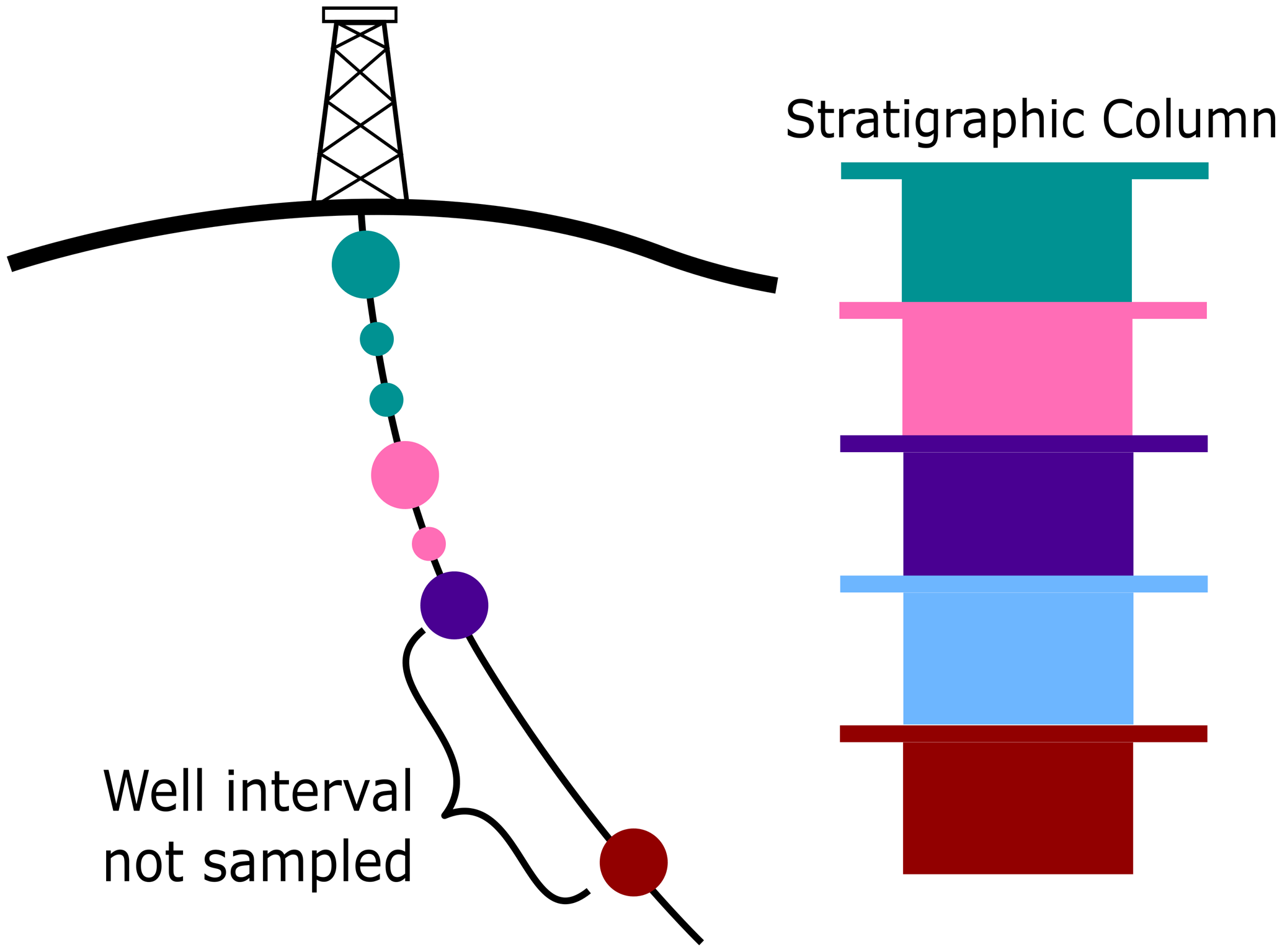
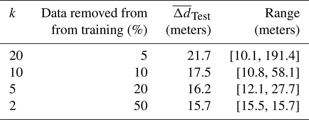
Table 2 GeoINR model performance metrics for case study 1.

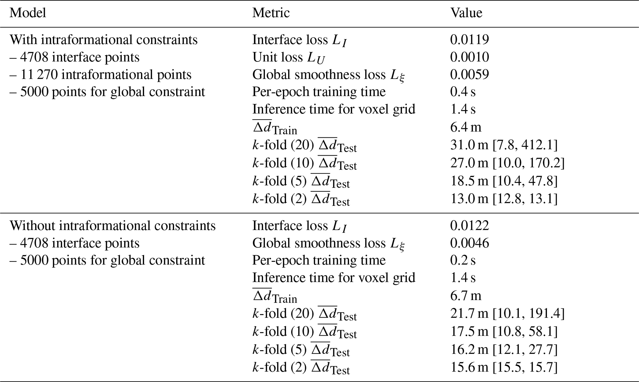
${\stackrel{\mathrm{‾}}{\mathrm{\Delta }d}}_X$ is the mean distance residual between modelled interfaces and point set X, either a training set or a test set. Brackets [] indicate the range of ${\stackrel{\mathrm{‾}}{\mathrm{\Delta }d}}_{\mathrm{Test}}$ values from a set generated by each k-fold cross-validation procedure.

The presented data and resulting models in Fig. 8 all have a vertical exaggeration of 100× so that the data and variation of geological structures can be visualized. For this dataset, the augmented intraformational points provided incremental refinements to modelled structures. An example of structural refinements is shown on a cross section taken from the middle portion of the model (Fig. 8c). The model made without the intraformational units (transparent curves) has the sub-Winnipeg unconformity (orange) positioned lower than it should since in that location there are no interface points sampling that unconformity. In addition, there are slight geometry changes for other interfaces with the model using intraformational units (solid curves) that are attributed to the presence of different units located off section. How the unconformities cut older stratigraphy and other unconformities can be clearly seen in modelled interfaces and resultant scalar fields in Fig. 8d, along with the visually impressive data fitting characteristics (also seen in Fig. 8b (left), c). The effect of adding the global smoothness constraint, or eikonal constraint (Eq. 18), can be seen in a scalar field associated with the youngest unconformity (φ⁴) shown in Fig. 8e (top). Without a global smoothness constraint, production of implicit modelling artifacts (e.g., isolated bubbles Fig. 8e (bottom)) can occur when paired with large training epochs and noisy datasets.

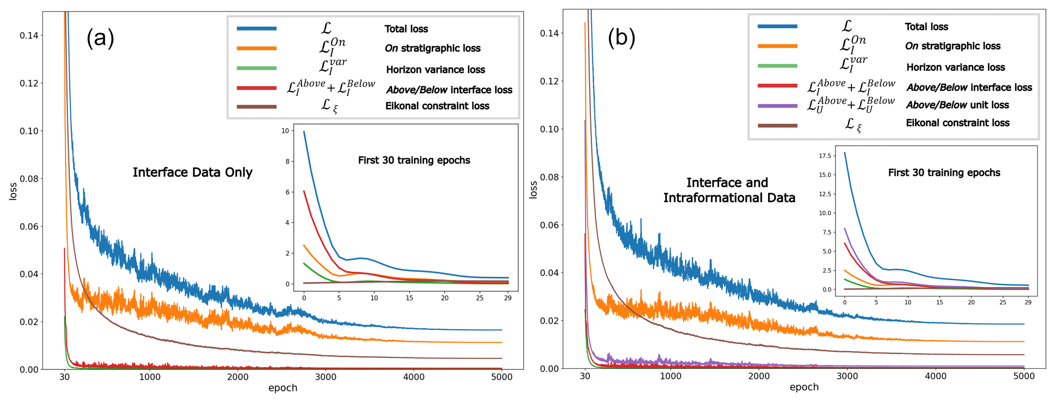
Figure 10 Loss function plots of constraints used for network training for the two sedimentary basin models produced using interface data only (a) and using both interface and intraformational data (b). Insets show loss function plots in the first 30 training epochs.

Resulting model performance metrics on both datasets used in this case study are summarized in Table 2. These metrics include loss function values at the last training iteration, computing times, mean distance residuals between modelled interfaces and associated point sets, and k-fold cross-validation results. Loss function plots for constraints used in the case study are provided in Fig. 10 to show how well they fit and their relative impact during network training. For the datasets used, the above/below stratigraphic relationship constraints significantly impact early (< 30 epochs) training dynamics so that modelled geological structures rapidly satisfy supplied knowledge constraints. In training epochs greater than 30, the total loss is more impacted by on stratigraphic and global smoothing (eikonal) constraints to locally refine and better fit modelled structures to individual observations. For computing times, per-epoch training times on one GPU led to a total of ∼ 35 min for the model with intraformational constraints and a total of ∼ 20 min without when using 5000 training epochs. A larger number of training epochs was chosen to achieve the smallest total error possible. However, even models generated with 1000 epochs were geologically representative of the basin but had larger fitting residuals. Note these computing times can be reduced by simply adding more GPUs and performing distributed training. The tabulated mean distance residuals, a real-world distance, were computed for the generated models using PyVista (Sullivan and Kaszynski, 2019) to give an intuitive notion of how well the GeoINR network fits the provincial-scale dataset. The mean distance residuals using the whole dataset, ${\stackrel{\mathrm{‾}}{\mathrm{\Delta }d}}_{\mathrm{Train}}$, were 6.4 and 6.7 m for the model including intraformational constraints and without, respectively. Most constraints had distance residuals near 0 m; however, some constraints had larger residuals; some data constraints exhibit a vertical shift upward in comparison to the other wells in the immediate vicinity surrounding the well. This could be due to faulting, highly variable localized structures, or misinterpretation. Finally, a systematic k-fold cross-validation (Rodríguez et al., 2009) analysis was completed to estimate the prediction error of the GeoINR network where there are no data available in the modelling domain and assess if the network suffers from overfitting. This analysis involved splitting the dataset into k partitions or “folds” and configuring them into k splits. For each split, the GeoINR network is trained using k−1 of the folds as training data using the same parameters in Table 1. Once the split is trained, the resulting model is validated on the remaining part of the data, called test data, where the mean distance residuals are computed. The mean distance residuals on the test data ${\stackrel{\mathrm{‾}}{\mathrm{\Delta }d}}_{\mathrm{Test}}$ are averaged over all splits and tabulated in Table 2. This procedure was performed for $k=\mathrm{20},\mathrm{10},\mathrm{5},\mathrm{2}$ and for both with and without intraformational constraints. From these results, it is evident that the GeoINR network has a reasonably low prediction error, especially given the provincial scale of the geological model, and the network does not suffer from overfitting. See Appendix C for a more detailed summary of the k-fold cross-validation results.

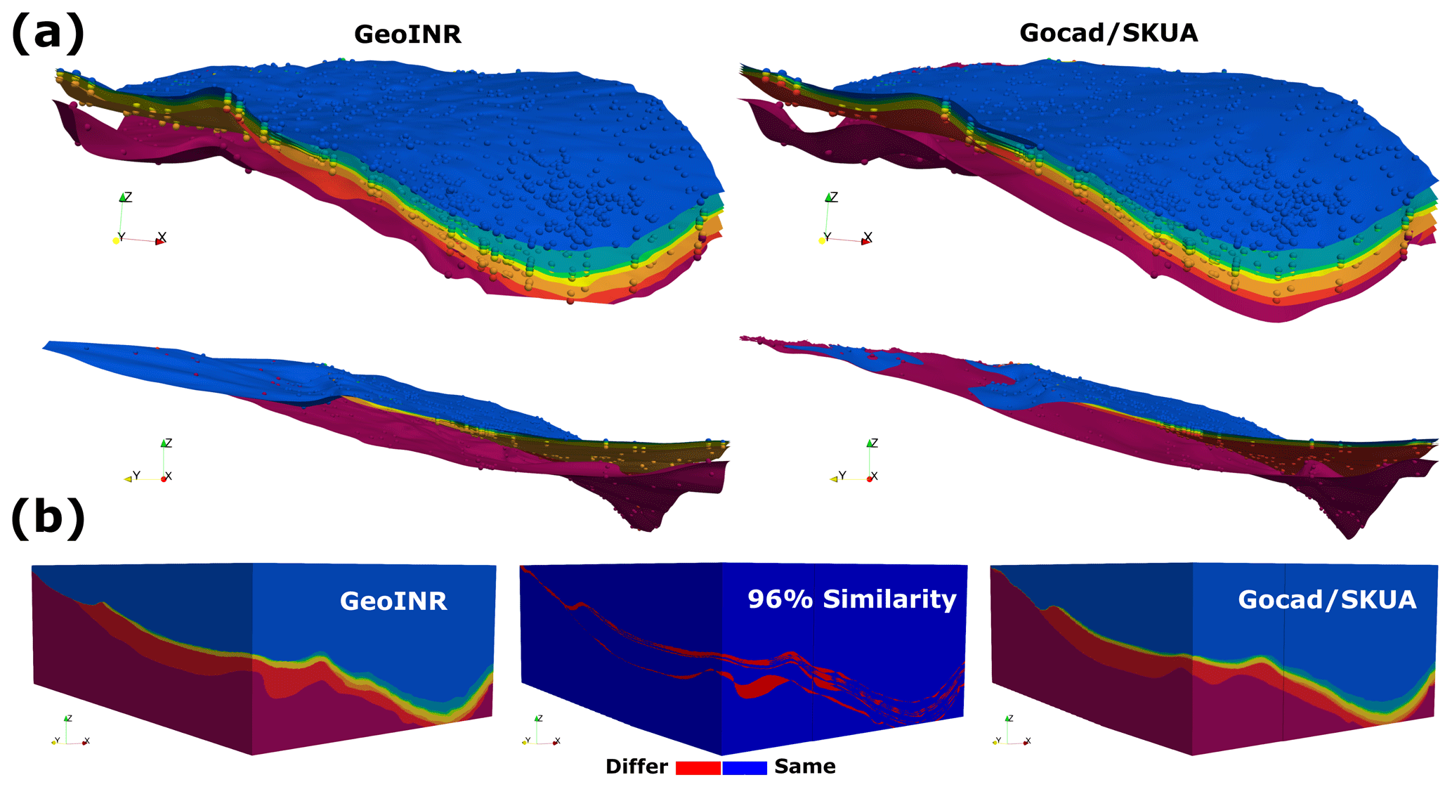
Figure 11 Similarity between the GeoINR model (left) for the Lower Paleozoic portion of the WCSB and the Gocad model (right) for the same region. (a) Modelled interface surfaces from two perspectives for both models. (b) Geological volume similarity between models.

In addition to the model performance metrics provided, we also present qualitative and quantitative comparisons of our three-dimensional geological model – constructed using interface and intraformational data – to a recent version of the model for the same region constructed using a hybrid implicit–explicit approach with Gocad/SKUA™ (geomodelling software) (Bédard et al., 2023). As shown in Fig. 11, it is clearly demonstrated that the developed methodology can produce geologically consistent modelling results since both models are so similar (96 %). The small differences (4 %) between them are attributed to the Gocad model using (1) updated top formation markers; (2) different interface relationships (e.g., erosional, onlap) for interfaces $I_{\mathrm{0}},I_{\mathrm{1}},I_{\mathrm{2}}$; and (3) extensive manual editing (e.g., explicit modelling) to refine implicitly modelled geometries to conform to depositional outlines available for each of the formations. Furthermore, it must be recognized that the similarity not only signals an excellent correspondence between models, but also supports the validity of both models through their cross-correlations; and the 4 % difference does not necessarily represent an error on either side, given the overall uncertainties of modelling over such a large area.

3.2 Regional outcrop case study

The second case study utilizes a regional-scale outcrop dataset from central Baffin Island, Canada (de Kemp et al., 2001; Scott et al., 2002; St-Onge et al., 2002). It consists of data from a deformed metamorphic setting having Archean-aged structural domes, composed of primarily felsic gneisses and plutonic rocks, that are basement to Paleoproterozoic rocks (Fig. 12a). The region is associated with a Himalayan-scale collisional mountain belt – the Trans Hudson Orogen – and consequently geologically complex. The dataset consists of 23 planar orientations (e.g., normals) sampled from the structural map (Fig. 12b), 352 geological unit (e.g., intraformational) observations (Fig. 12c), and 6 interface observations (Fig. 12d). While the geological unit and orientation observations were taken in the field, the limited number of interface observations were randomly sampled from the geological map. For this case study, the objective is to demonstrate that the developed methodology can generate representative three-dimensional geological models from typical outcrop datasets: i.e., with limited interface data, moderate geological unit information, and orientation observations. The resulting three-dimensional geological models are validated by visually comparing the modelled objects with the generalized geological source map (Fig. 12c) of the structural domes (red – Na-g), the onlapping quartzite (yellow – Pp-PD), and the overlying units (blue – Pp-PL). To facilitate comparison, the three-dimensional modelling results (Fig. 12e, f (right)) are clipped at the topographic surface (Fig. 12e, f (left), g).

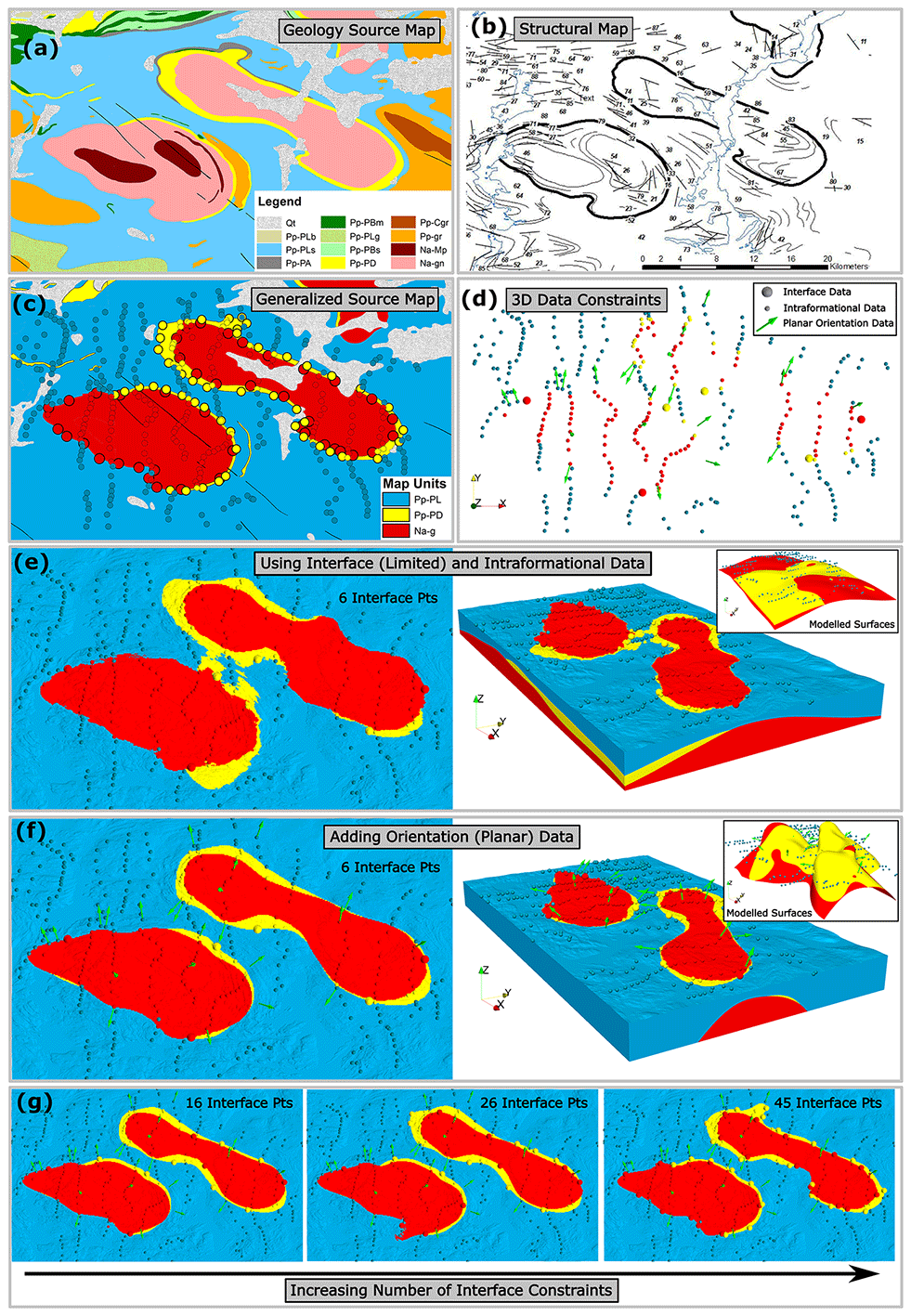
Figure 12 Modelled geological map patterns using the outcrop dataset in a deformed metamorphic setting containing structural domes (red) and onlapping quartzite (yellow). (a) Geology source map for region of interest. (b) Structural map of available orientation observations. (c) Three-class generalized source map. (d) Three-dimensional data constraints. (e) Results using only limited interface and moderate intraformational data. (f) Results adding orientation data. Insets are extracted modelled interface surfaces. (g) Results from increasing number of interface points.

Three sets of modelling results are presented. First, only the limited interface and moderate intraformational data are used (Fig. 12e). The resulting modelled map pattern with these data closely matches the expected pattern on the generalized map (Fig. 12c). Second, in Fig. 12f, the sampled orientation observations were added, resulting in an even better match: the quartzite (yellow) between the two domes (red) is no longer connected. Note that the addition of orientation data strongly influenced modelled geometries, which then better conforms to the observed orientational data. Third, in Fig. 12g, the addition of more interface points (sampled from map contacts) results in only minor model refinement. This case study, therefore, demonstrates the ability to successfully model a complex geological scenario with limited interface data, which is typical of outcrop datasets.

Table 3 GeoINR model performance metrics for case study 2.

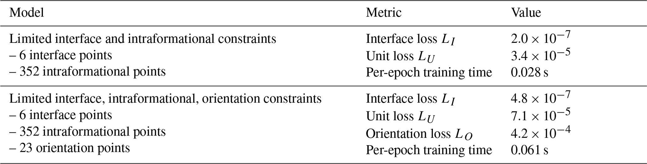
Quantitatively, model performance metrics for this case study are summarized in Table 3. Note that the global smoothness constraint L_ξ was not used during training. This was because the dataset did not require smoothing since there was minimal data noise (e.g., nearby observations are geologically consistent). In addition, note from the summarized metrics it is possible to achieve near-exact fitting (e.g., total loss < 0.0001 after 2000 training epochs) while maintaining geologically reliable models. Finally, detailed loss plots (Fig. D1) are provided in Appendix D for those interested in a deeper understanding of the impact of individual loss functions for all geological models generated.

4 Discussion

Our results show INR networks can be successfully applied to a diverse range of geological settings, using well and outcrop datasets. In the first case study (Sect. 3.1), these networks were shown to be capable of generating large-area basin-scale models containing numerous unconformities and conformable stratigraphic interfaces from large and noisy well datasets. While the intraformational constraints only provided incremental improvements to the basin model, they did help demonstrate their compatibility with the methodology. However, these types of constraints proved to have much more impact on modelling with outcrop datasets, which have significantly fewer interface points (Sect. 3.2). They could also provide a mechanism for better leveraging geological maps in the modelling process by incorporating points sampled within unit polygons and appropriately weighting them in loss functions. Finally, it is clear, though unsurprising, that orientation constraints can strongly influence and improve modelled geometries of geological structures, especially in highly deformed geological settings and sparse-data scenarios.

The ability of INR networks to process above and below inequality constraints on stratigraphic relations (Eqs. 4, 7, 8) shows these networks can efficiently incorporate atypical knowledge constraints derived from stratigraphic columns and geological rules (e.g., erosion, onlapping). In comparison, classical implicit interpolation methods must solve computationally expensive convex optimizations in order to incorporate such constraints, resulting in poor scaling as the number of constraints increases. Moreover, these classical methods only apply inequality constraints to a single scalar field, to the best of the authors' knowledge, and not across a series of scalar fields. In contrast, neural networks do not need to solve such expensive optimizations and can efficiently couple a series of scalar fields to apply constraints across them, thus enabling improved integration of knowledge.

Iso-values associated with modelled interfaces in the proposed methodology vary in every training iteration of the learning algorithm, so modelling results are independent of user-defined iso-values. While defining specific interface iso-values is a straightforward way to encode the stratigraphic sequence (e.g., larger values are younger than smaller values), it is not optimal. Assigning specific iso-values for interfaces heuristically (e.g., uniformly distributed between some numerical range) can negatively impact resulting modelled geometries. This is particularly evident when dealing with varying unit thicknesses across the modelling domain and many interfaces. However, the GeoINR algorithm avoids these issues by learning the optimal set of interface iso-values during training, thus permitting more complex geological structures to be modelled. It is important to note that the stratigraphic constraints (Sect. 2.4.1) embed the knowledge of the stratigraphic sequence, with resulting interface iso-values respecting that sequence.

Loss functions used to constrain resulting implicit scalar functions make frequent use of scalar field gradients ∇φⁱ computed on point sets. To compute the gradient of a scalar field generated by an implicit function parameterized by a neural network for an input point, the chain rule is applied to the networks output, φⁱ(x), with respect to the coordinates of the point $\mathit{x}=\left(x,y,z\right)$. An advantage of machine-learning programming frameworks (PyTorch, TensorFlow) is the straightforward and efficient method of gradient computation, which requires only one line of code. Note that higher-order nth derivatives may also be similarly computed (e.g., useful for Laplacian or curvature computations) provided that the non-linear activation function σ is at least n times differentiable.

Although the MLP network architecture parameters ($N_{\mathrm{h}},d_{\mathrm{rep}},\mathit{\sigma })$ used in this contribution (Table 1) generated reliable and accurate three-dimensional modelling results, the architecture may not be optimal for all geological scenarios. As a general principle, increasing the number of hidden layers N_h tends to improve the capacity of the network to model more complex structures, whereas increasing the dimensionality of representations d_rep (number of the neurons in a layer) tends to improve the smoothness of modelled geometries (Hillier et al., 2021). But these effects have diminishing returns as these parameters are further increased. It is important to note that the use of different non-linear activation functions σ can dramatically affect modelled geometries. Empirically, we tested all currently available activation functions within the PyTorch framework and found the two most reliable activation functions were ReLU and Softplus. In this paper, we used a parameterized Softplus activation function that generated far smoother geometries and improved data fitting compared to the commonly used ReLU. ReLU activation functions typically result in modelled geometries with sharp creases, which could be more useful in brittle geological settings. In scenarios where these architectural parameters are not ideal, automated tools are available for optimizing them (Liaw et al., 2018). In general, the best architecture to use for a particular geological scenario is an open research question. This motivates the development of standardized three-dimensional geological models to be used for benchmarking different methods and their parameterizations.

Several interesting points arise from comparing the GeoINR and GNN deep-learning approaches (Hillier et al., 2021) for three-dimensional geological modelling. First, the generation of latent representations (e.g., embeddings, features) in GeoINR is at a minimum 2 orders of magnitude faster than in GNNs. Second, GeoINR does not require the generation of an unstructured volumetric grid (e.g., tetrahedral mesh), enabling the development of higher-resolution models over larger areas. For example, for the provincial case study, the GNN tetrahedral mesh with varying resolution required ∼ 10 GB of storage, whereas the GeoINR voxel grid with a high resolution in vertical dimension required only ∼ 150 MB of storage, resulting in significant computational efficiencies. Lastly, the GeoINR models seemed superior as the scalar fields generated by GNNs were much noisier, as the graph-based convolution operations did not seem to adjust as effectively during network training. For GNNs to provide meaningful improvements to structural modelling, the graph structure must represent meaningful geological concepts and not simply something on which a scalar value is predicted (e.g., tetrahedral mesh).

In other future work, we aim to tackle various discontinuous features commonly found in more complex orogenic and shield terrains, such as faults and shear zones. Because neural networks with similar architectures have shown the capacity to approximate discontinuous functions (Llanas et al., 2008; Santa and Pieraccini, 2023), we believe GeoINR should support the modelling of these complex features with appropriate enhancements and modifications (e.g., discontinuous activation functions).

INR networks have been reported as underrepresenting high-frequency components of signals and shapes by underfitting these components (Mildenhall et al., 2021). Positional encodings are a common strategy for addressing this issue by transforming the coordinates of a point into a set of Fourier features, which are then fed into the hidden layers of the network (Tancik et al., 2020). Our preliminary tests indicate that while this technique improved local fitting of high-frequency detail when using either ReLU or Softplus activation functions, it can generate unsupported large wavelengths of folded features.

5 Conclusions

We have introduced GeoINR, a geological modelling approach founded on INR networks composed of MLPs. GeoINR advances an existing INR approach by incorporating unconformities, constraints for stratigraphic relations and global smoothness, and improved training dynamics from the geometrical initialization of network variables. These advances enable efficient modelling of more complex geology, improved data fitting, and reductions in the generation of modelling artifacts. Case studies demonstrate the effectiveness and validity of the approach in diverse geological settings, different-sized areas, and various data regimes. Future work will extend GeoINR to support modelling of even larger datasets in more complex geological settings involving faulting and intrusions.

Appendix A: Iso-surface extraction algorithm

Appendix B: Interface and formation unit information for case studies

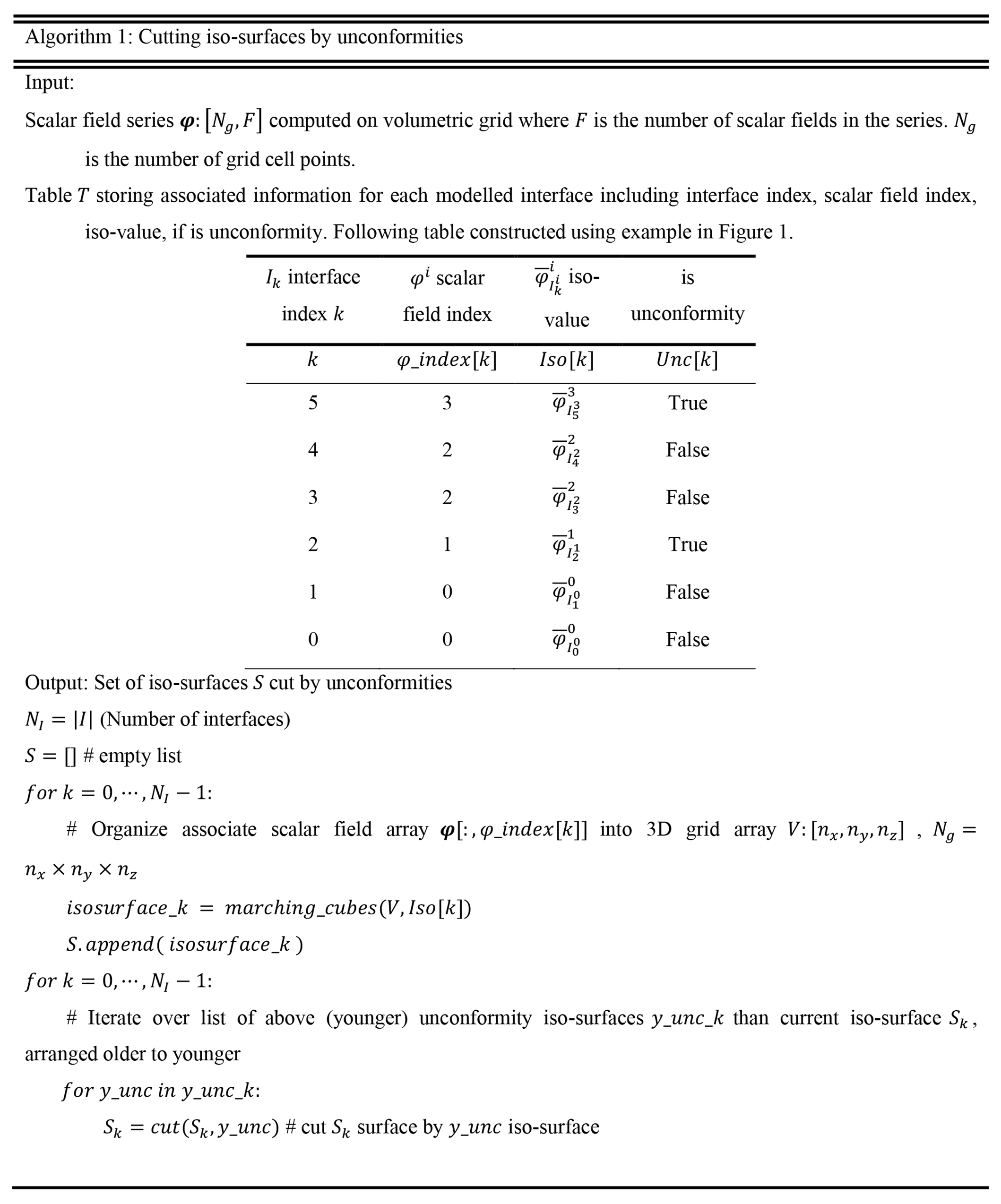
Table B1 Interface information for case study 1. n/a denotes not available.

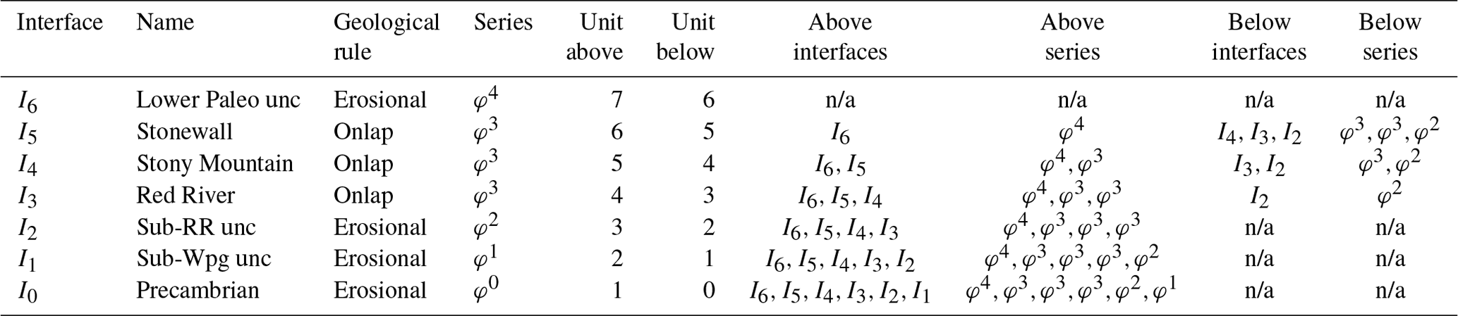
The sequence of the above/below interface and series are associated. For example, consider the below interfaces and series for I₅. Interface I₄ is associated with series φ³. Similarly, interface I₃ is associated with series φ³, and interface I₂ is associated with series φ². Lower Paleo unc: Lower Paleozoic unconformity; sub-RR unc: sub-Red River unconformity; sub-Wpg unc: sub-Winnipeg unconformity.

Table B2 Formation unit information for case study 1. n/a denotes not available.

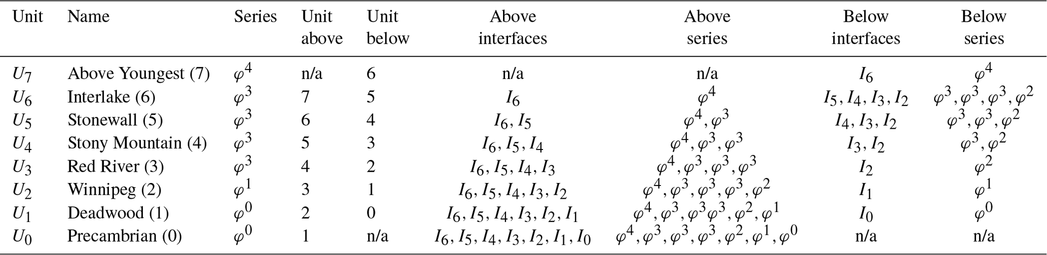
Table B3 Interface information for case study 2. n/a denotes not available.

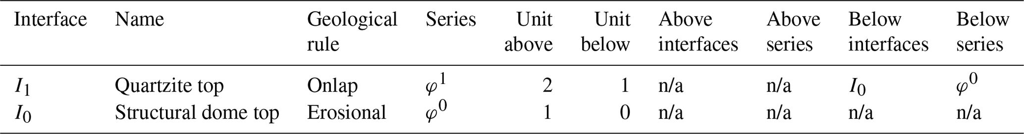
Above/below interfaces and series indicated here use the efficient option for stratigraphic relations mentioned in Sect. 2.4.1.

Table B4 Formation unit information for case study 2. n/a denotes not available.

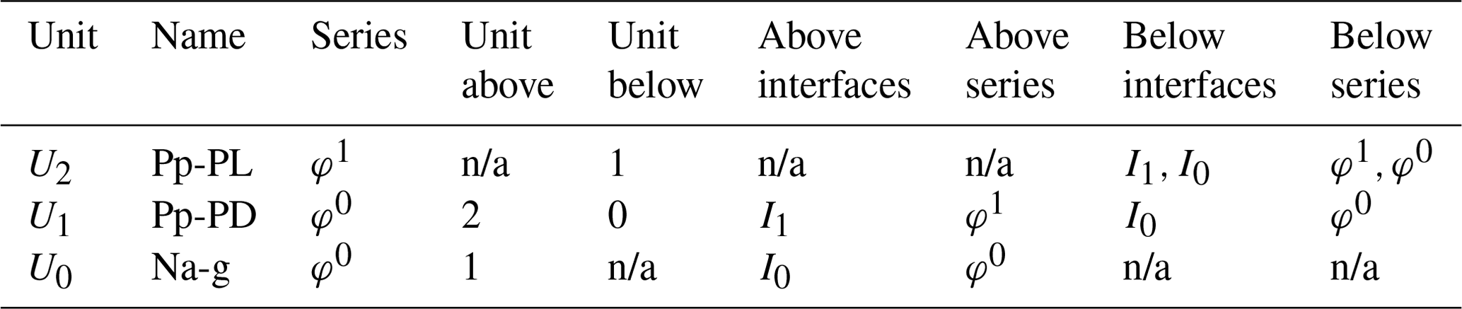
Above/below interfaces and series indicated here use the efficient option for stratigraphic relations mentioned in Sect. 2.4.1.

Appendix C: k-fold cross-validation results for case study 1

See https://scikit-learn.org/stable/modules/cross_validation.html (last access: 17 November 2023) for implementation details and illustration regarding the k-fold cross-validation procedure. The range of mean distance residuals on test points, ${\stackrel{\mathrm{‾}}{\mathrm{\Delta }d}}_{\mathrm{Test}}$, from all k splits indicates the lower and upper bound of these residuals across all splits for a given k. The large mean residual for upper bounds (e.g., 191.4 m for k=20 in Table C2) is the result of a single point constraint associated with the sub-Winnipeg unconformity in the far north-west corner of the modelling domain. For every k-fold procedure carried out, there is always one split point that is excluded from training and results in a larger mean distance residual, and it increases with larger k, on the corresponding test set. It is important to note that the next nearest constraint to this point associated with this interface (sub-Winnipeg unconformity) is 150 km away. The upper bound on mean distance residuals decreases with smaller k. This is because with smaller k a higher percentage of constraint points are removed from training, and generated models become more generalized. The lower bound of mean distance residuals decreases with larger k, since more points are used to constrain generated models.

Table C1 k-fold metrics for the structural model generated from interface and intraformational constraints.

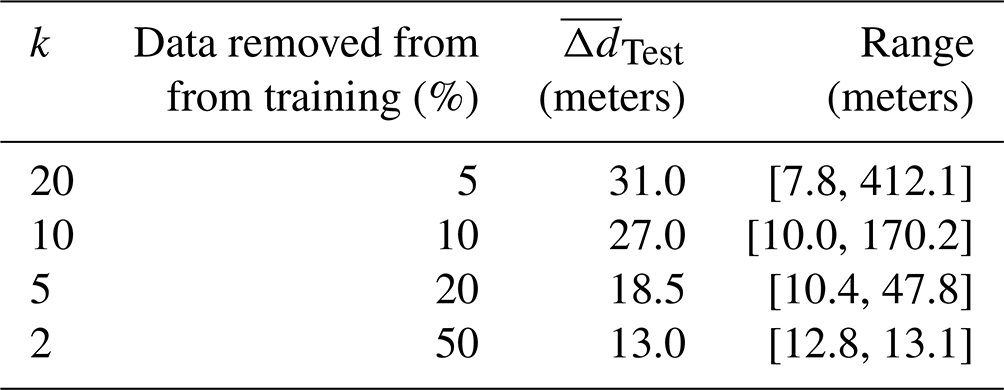
Table C2 k-fold metrics for the structural model generated from interface constraints only.

${\stackrel{\mathrm{‾}}{\mathrm{\Delta }d}}_{\mathrm{Test}}:$ mean distance residual computed on the testing set (not used to train/fit the model).

Appendix D: Loss function plots for case study 2

Note the following from loss plots shown in Fig. D1: (1) when no orientation data are used in training (Fig. D1a), early training is strongly influenced by the stratigraphic constraints (on, above, below) imposed on interface data, whereas all other models (Fig. D1b, c, d, e) are strongly influenced by the orientation data. (2) Beyond 50 epochs, training is influenced by on stratigraphic constraints, followed by orientation constraints and then above/below constraints on intraformational data.

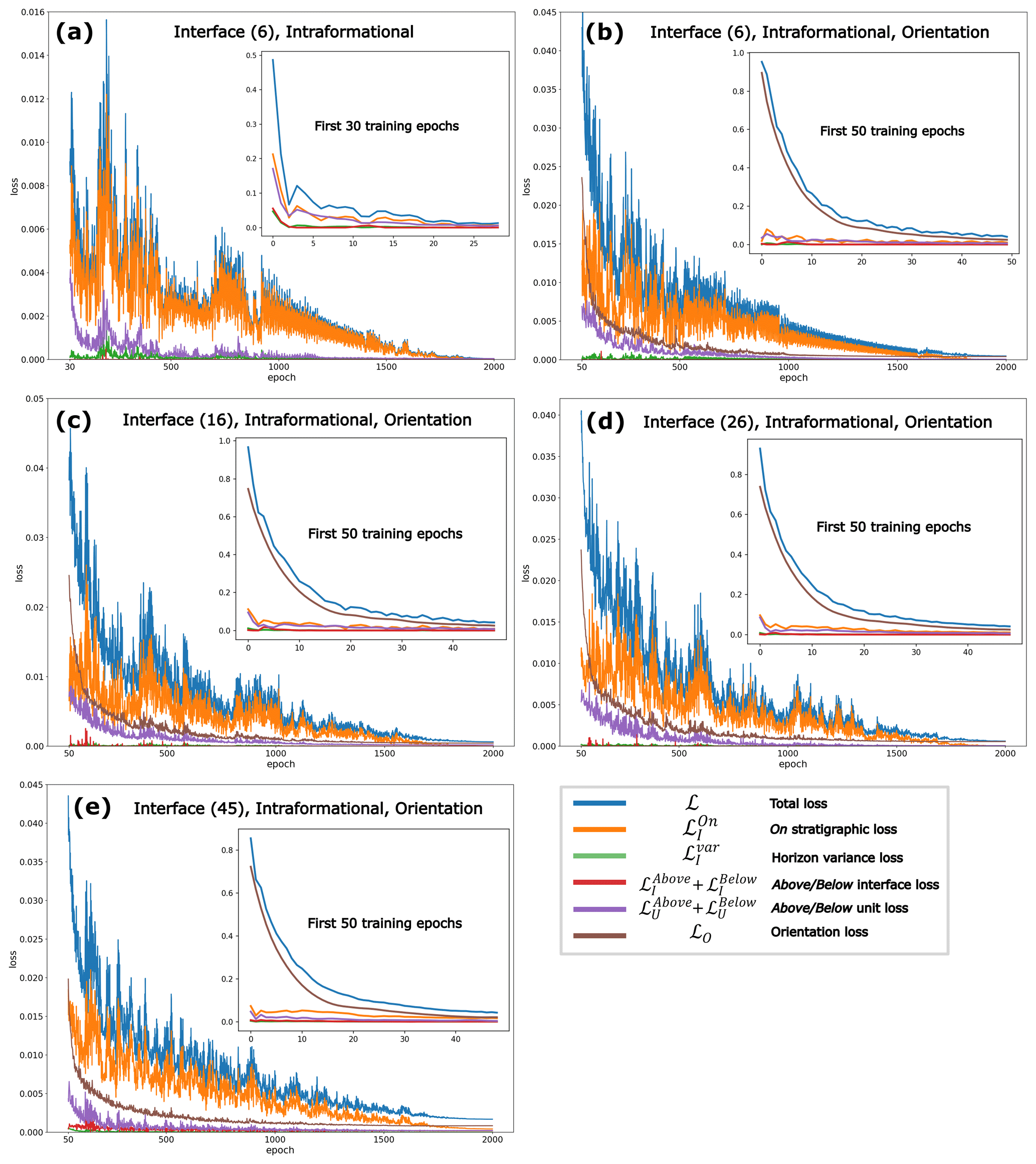
Figure D1 Loss function plots as function of training epoch for individual constraints used in case study 2. (a, b, c, d, e) Plots corresponding to generated geological models shown in Fig. 12 (e, f, g (left), g (middle), g (right)), respectively.