the Creative Commons Attribution 4.0 License.
the Creative Commons Attribution 4.0 License.
 | 29 Nov 2023
AdaScape 1.0: a coupled modelling tool to investigate the links between tectonics, climate, and biodiversity
Esteban Acevedo-Trejos
Jean Braun
Katherine Kravitz
N. Alexia Raharinirina
Benoît Bovy
The interplay between tectonics and climate is known to impact the evolution and distribution of life forms, leading to present-day patterns of biodiversity. Numerical models that integrate the co-evolution of life and landforms are ideal tools to investigate the causal links between these earth system components. Here, we present a tool that couples an ecological–evolutionary model with a landscape evolution model (LEM). The former is based on the adaptive speciation of functional traits, where these traits can mediate ecological competition for resources, and includes dispersal and mutation processes. The latter is a computationally efficient LEM (FastScape) that predicts topographic relief based on the stream power law, hillslope diffusion, and orographic precipitation equations. We integrate these two models to illustrate the coupled behaviour between tectonic uplift and eco-evolutionary processes. Particularly, we investigate how changes in tectonic uplift rate and eco-evolutionary parameters (i.e. competition, dispersal, and mutation) influence speciation and thus the temporal and spatial patterns of biodiversity.
- Article
(6133 KB) - Full-text XML
- BibTeX
- EndNote


Tectonic, climate, and evolutionary processes share an intrinsic co-evolutionary history (Lenton, 2004), which leaves salient patterns in the evolution and spatial distribution of life forms we observe today. For example, high biodiversity observed in mountain regions suggests a link between tectonics, climate, and the evolution of life forms (Fjeldså et al., 2012; Rahbek et al., 2019b, a). The Andean uplift led to increased topographic complexity and changes in climate (Hoorn et al., 2010), which prompted and sustained biodiversity in plants (Böhnert et al., 2019; Martínez et al., 2020; Pérez-Escobar et al., 2022), frogs and lizards (Boschman and Condamine, 2022), as well as fishes (Cassemiro et al., 2023). Similarly, a link between topographic complexity, associated climate changes, and high biodiversity have been proposed in highly diverse regions such as the Tibet–Himalaya–Hengduan region (Spicer, 2017; Ding et al., 2020) and tropical Africa (Couvreur et al., 2021). However, we do not fully understand how tectonics and climate influence macroecological and macroevolutionary processes on large spatial and temporal scales. This requires a combination of approaches from multiple disciplines across the bio- and geosciences (Antonelli et al., 2018).
Understanding the large-scale temporal and spatial variation of life forms has been one of the central themes in various fields of ecology and evolution, such as macroecology (Brown and Maurer, 1989; McGill, 2019), historical biogeography (Wiens and Donoghue, 2004), macroevolution (Condamine et al., 2013), and more recently functional biogeography (Violle et al., 2014). Given the challenge of studying systems at such broad scales, these fields have utilised the use of simulation models to link ecological and evolutionary processes in a spatially explicit context (Grimm et al., 2005; Gotelli et al., 2009; Connolly et al., 2017; Cabral et al., 2017). Currently, these types of models are known as “population-based spatially explicit Mechanistic Eco-Evolutionary Models”, or MEEMs (Hagen, 2022), and prominent examples include Rangel et al. (2018) and Hagen et al. (2021a). In these models, the main emphasis is on how species interact and evolve, in a grid-based environment, where environmental fields (e.g. topography, temperature, and precipitation) are representations of past or present features computed a priori. These landscape representations are provided by other models, such as global palaeo-elevation reconstructions (e.g. as in Hagen et al., 2021a) or after reanalysis of the output of other models (e.g. as in Rangel et al., 2018). These MEEM tools offer flexibility in the inputs and detail treatment of the ecological and evolutionary processes; however, they provide little control over the mechanisms that generate climate and landforms.
Simulating landforms requires considering tectonics, climate, and erosional processes, where particularly the latter can be mediated by organisms (Viles, 2020). Similarly, as in large-scale ecology, we can also investigate the processes leading to the formation of a particular topography using landscape evolution models (LEM) (Tucker and Hancock, 2010). But despite much progress in the field of biogeomorphology, there is a need for a new generation of LEMs, to function as a type of “multipurpose modelling toolkit” as suggested by Viles (2020), that will integrate landscape as well as ecological and evolutionary processes at large spatial and temporal scales (Badgley et al., 2017; Antonelli et al., 2018; Rahbek et al., 2019a). Nevertheless, such a toolkit should be simple enough to maintain generality while capturing the relevant processes in macroecology, macroevolution, and geomorphology.
Here we present AdaScape, a coupled speciation and landscape evolution model conceived as a simple eco-evolutionary component built into an established LEM framework known as FastScape (Bovy, 2021). The modelling framework is implemented in the programming language Python and provides spatially explicit environmental fields, e.g. topography and rainfall, while the AdaScape component contains routines to compute the adaptive speciation of individuals within the environment, which builds on the adaptive dynamics theoretical framework (Metz et al., 1996; Geritz et al., 1998; Dieckmann et al., 2004, 2007; McGill and Brown, 2007; Brännström et al., 2012). Organisms in such eco-evolutionary models are characterised by their traits and a fitness function that relates their trait values to local environmental conditions (McGill et al., 2006; Webb et al., 2010); thus, the traits are not simply an input or a parameter of the model but a dynamic variable predicted by the model (Klausmeier et al., 2020). Below we describe in detail AdaScape and briefly FastScape, and provide a simple example to showcase the main features of the coupled modelling tool.
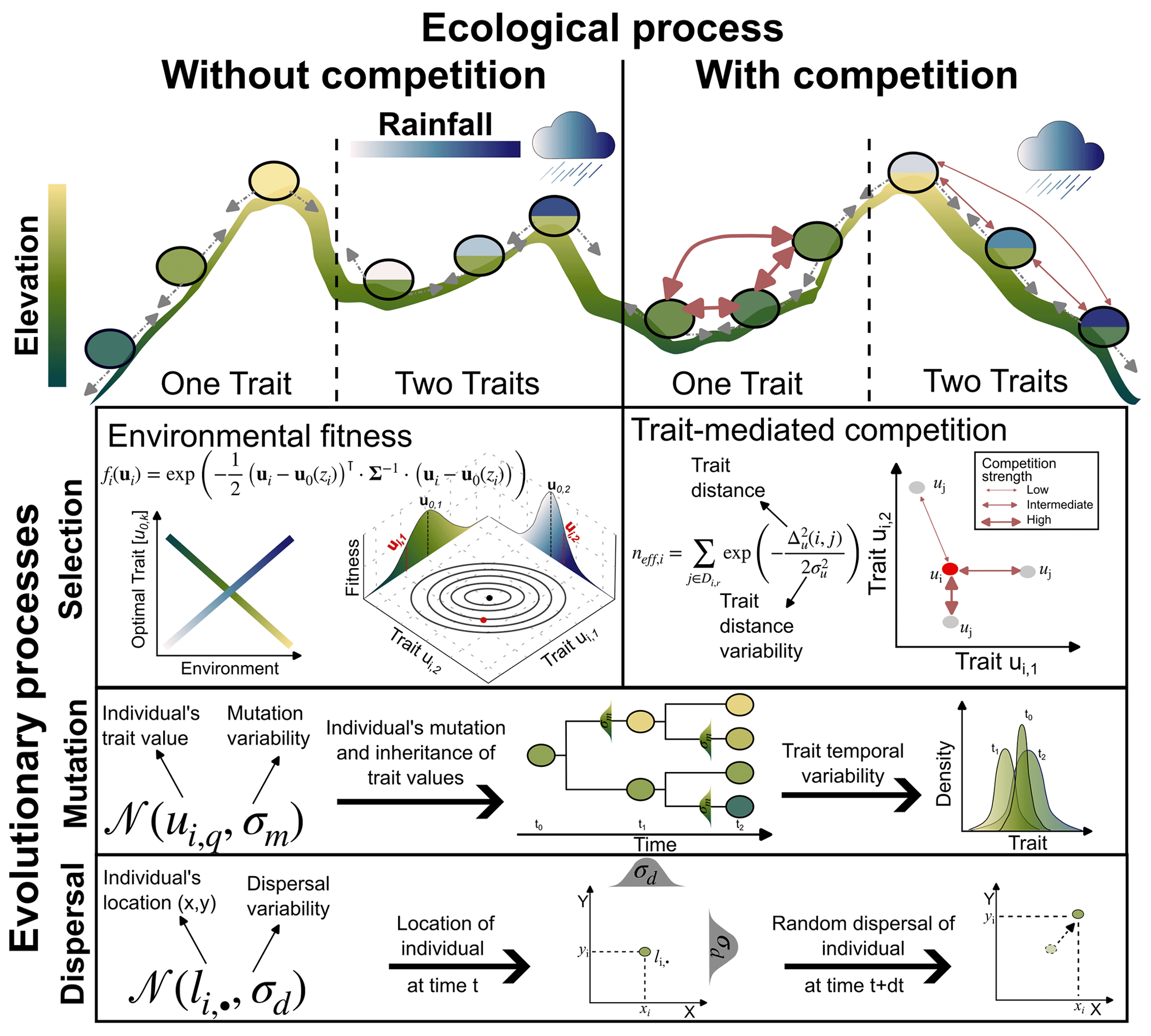
Figure 1Illustration of the main ecological and evolutionary processes included in AdaScape for two traits (i.e. k=2) representing the adaptation of the population to topographic elevation and to rainfall, respectively. The eco-evolutionary model is a modified version of the one proposed by Irwin (2012). Selection is one of the crucial eco-evolutionary processes included, which is here determined by the environmental fitness or how suitable the trait values of an individual compare with the optimal trait value for a given local environmental condition, zi. The other main selection process is trait-mediated competition, which determines how many individuals with similar trait values to the focal individual i are competing for the same local resource. We also include mutation and dispersal as stochastic processes that depend, respectively, on the trait and location of the individual i and the parameters that control the variability or width of the trait value (σm) and location (σd) the offspring will inherit or to which they will be dispersed.
AdaScape is built on the simple eco-evolutionary model proposed by Irwin (2012), which describes the trait evolution of a group of individuals with processes related to environmental selection, mutation, and dispersal (Fig. 1). We extend this model to include (a) competition of a limiting resource influenced by individual traits, and (b) more than one trait, which are related to environmental fields such as elevation and rainfall via simple linear function. The latter are environmental fields provided by a landscape evolution model (Fig. 1 and Sect. 2.5). Below we describe in detail the evolutionary and ecological components included in AdaScape as well as the taxon definition we use to reconstruct phylogenies and the basic elements needed to predict landscape evolution as included in FastScape.
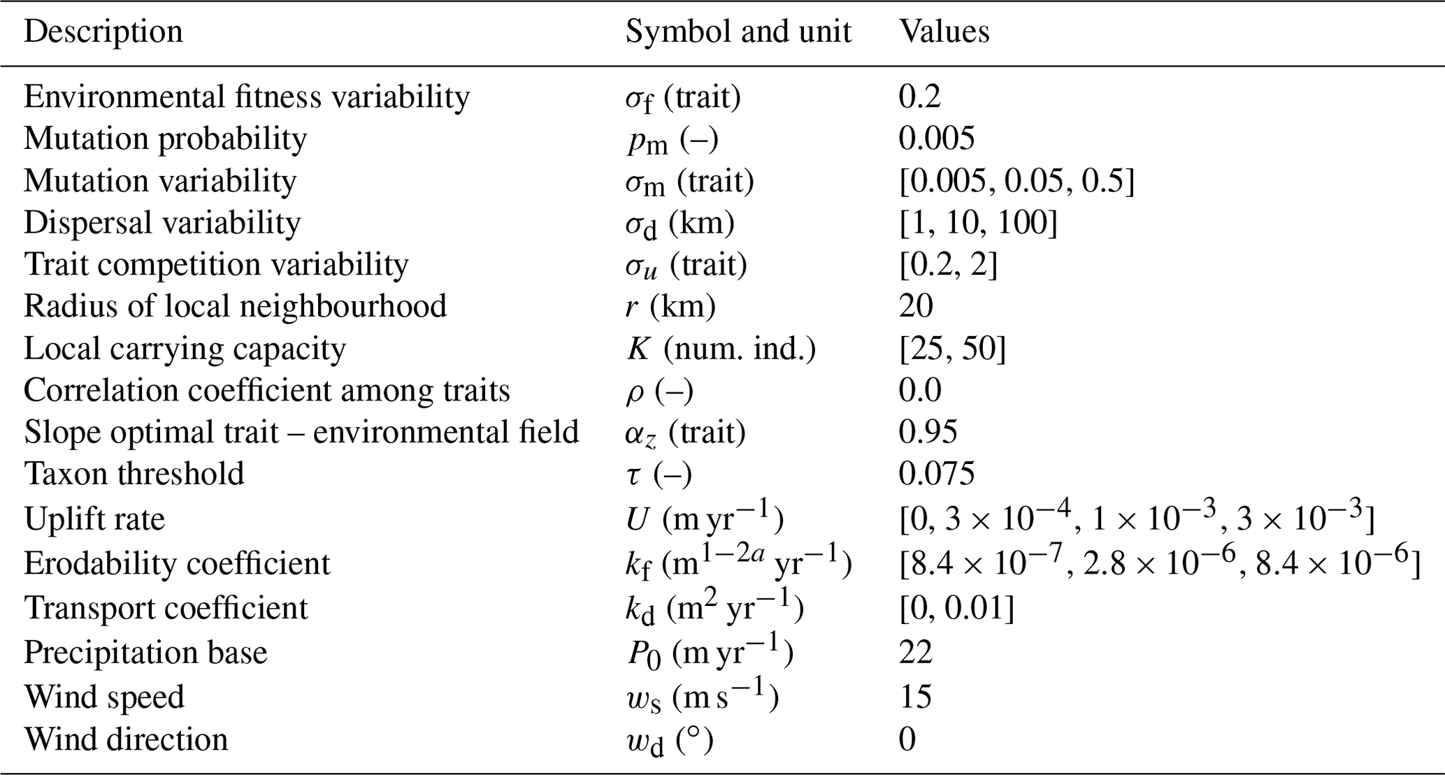
Table 1Description of parameters in the adaptive speciation model, together with a selection of parameters we vary to reconstruct the topography and rainfall patterns. We use the default values for all other parameters in the landscape evolution and orographic precipitation model. Num. ind.: Number of Individuals.
2.1 Evolutionary components
Individuals i are characterised by a vector of trait values ui of length corresponding to the number of traits k, that is, . Environmental fitness (Fig. 1) is given by a multivariate Gaussian function fi, which reduces the fitness gain of the individual as its trait vector moves away from the optimal trait value vector u0(zi), where for a given local environmental condition zi as
where Σ is the k×k matrix of parameters driving the fitness changes. Each diagonal element, σq,q, on the matrix Σ parameterises the fitness changes independently generated by the trait ui,q for all . We assume that these diagonal elements are equal to σf for all traits (Table 1). The parameter σf determines the strength of the selection of an individual's trait value against its optimum and is hereafter referred to as the environmental fitness variability. Each off-diagonal elements of Σ, denoted σq,r, parameterises the fitness change jointly generated by the pair of traits at position q and r of the trait vector ui, for all such that q≠r. We define for all q≠r to model the interdependent effect that traits ui,q and ui,r have on fitness. The parameter ρ, thus, is set to zero here to simulate independent effects of all traits (Table 1).
The optimal trait value of the qth trait is given by a trait–environment relationship. Following Doebeli and Dieckmann (2003), we set this relationship to be linear:
where αz is a free parameter determining the slope of the relationship (Table 1) and Zi is the normalised environmental conditions experience by individual i. We use a normalised environmental field as these fields can change during the simulation. To facilitate the parameterisation, the ranges for an environmental field must be set up before the execution of the eco-evolutionary model. Therefore, one can use the maximum zmax and minimum zmin ranges that each environmental field can reach during a simulation or the known ranges for a particular taxon or clade. The full expression for Zi(zi) is given by
Mutation is the second evolutionary process we consider (Fig. 1), which is described as an intergenerational stochastic variation of the trait values. The mutation process is thus modelled as a stochastic process occurring at probability pm at every generation time. This process is typically simulated using a simple Monte Carlo sampling algorithm. The algorithm draws a random number from a uniform distribution 𝒰(0,1) and compares it with a mutation probability pm (Table 1). If the drawn number is less than pm, then the descendant of the individual i can mutate. Now a mutation is characterised by a new trait value taken from the Gaussian distribution centred at the ancestor trait value ui,q and with a mutation variability σm (Table 1).
The nature of the mutation process is more complicated than the simplification given here and can be defined in its broadest sense as a heritable change in the genome, which can be measured as the number of base pair substitutions per generation and is positively related to the genome size of the organism (Lynch, 2010). Changes in the genotype could lead to phenotypic variation that may be positively or negatively influenced by natural selection, and therefore mutations could be silent, advantageous, or deleterious (Bromham, 2016). Our model simplifies this genetic–phenotypic complexity by assuming that a change in the genotype (via mutation) directly corresponds to a change in the phenotype (trait), the latter of which is subject to selection and transmitted by uniparentally inherited markers (in the absence of sexual selection) as in Irwin (2012).
The third evolutionary process we consider is dispersal (Fig. 1), where the new location of an individual i is randomly sampled around the position of each individual li,x and li,y, along the x and y axes using separated Gaussian distribution , where • is a place holder for x or y. Individuals' dispersal ability is influenced by their dispersal variability σd (Table 1), which is considered here as a free parameter. In other words, dispersal describes the random movement of individuals and their traits through the landscape, where the new location of individuals at t+1 depends on the location of individuals at time t and σd.
2.2 Ecological component
The main ecological interaction we consider in AdaScape is via a trait-mediated competition (Fig. 1). In the original model of Irwin (2012) all the individuals nall in the local neighbourhood were assumed to compete for a local resource. The latter can sustain a given number of individuals, or local carrying capacity K (Table 1). The extent of the local neighbourhood is defined by a radius r (Table 1) and is centred at each individual location. We modify this assumption by accounting not only for all individuals in the local neighbourhood but specifically for those individuals with similar trait values to the centred individual i. For this, we introduce a term to account for the effective number of individuals neff,i similarly to Doebeli and Dieckmann (2003). The expression accounting for the trait-mediated competition is given by
where Di,r is the local neighbourhood of radius r of individual i, Δu(i,j) is the trait distance between individual i and its neighbour j, and σu is trait-distance variability or width (Table 1). The local neighbourhood is the area around each individual centred at its location and with an extent determined by r and can be thought of as the area where local competition for resources take place. The parameter σu dictates the strength of the competition among individuals with similar trait values. Hence, if σu≥1, all individuals in the local neighbourhood, regardless of their trait values, are assumed to compete for the same resource. However, if σu<1, only those individuals with similar trait values to the focus individual i are counted and thus assumed to compete for the same resource. In other words, the similarity in trait values is determined by how small σu is. Hereafter we consider two contrasting cases of this process that we define without (σu=2) and with (σu=0.2) trait-mediated competition.
2.3 Implementation details of the eco-evolutionary model
The model is implemented as an individual-based, spatially explicit model in Python. A simulation is initialised with a given number of individuals allocated randomly or at a particular range in a continuous 2D space. The traits for each individual are drawn from a uniform distribution, where the minimum and maximum range is between 0 and 1. In all simulations hereafter we start with a monomorphic population, i.e. all individuals descend from the same ancestor and share similar trait values. After initialisation, the fitness for each individual is evaluated following Eq. (1). Then we compute the number of offspring noff,i for each individual i following Irwin (2012) using
where the is the density-dependent reproductive factor. After the number of offspring has been determined, the new individuals are generated, mutated, and dispersed. The two latter are implemented as stochastic processes as explained in the previous section. This model thus assumes that a generation is completed after all individuals have been updated; therefore, generations do not overlap.
2.4 Taxon definition
We define a taxon as a group of individuals sharing similar trait values and common ancestry (sensu Pontarp et al., 2012). We implement this by using a spectral clustering algorithm (von Luxburg, 2007), which examines individuals per ancestor group and assigns them to new taxon groups based on the clustering of their trait values at each time step. To each of these clusters we assigned a new taxon ID , and this taxon ID at time t will become the ancestor ID at time t+1. For example, if one assumes that all individuals share a common ancestor and all of them have very similar trait values (a monomorphic population), then branching does not occur and all individuals will be assigned to a single taxon ID (e.g. equal to 1 if the ancestor ID is equal to 0). Conversely, if the clustering algorithm found two distinct trait clusters, then branching occurs and the individuals are clustered into two new taxon groups with different IDs (e.g. 1 and 2 if the ancestor ID is equal to 0); with this we are avoiding polytomies by considering only binary splits. At the next time step and after the calculation of the eco-evolutionary processes (see details above), the previous taxon ID becomes the ancestor ID, and we apply the spectral clustering algorithm again using the new ancestor group. In our simulations, we restricted the division of taxa to a maximum of two to avoid the excessive occurrence of branching. Additionally, to add more interpretability to our taxa clusters, we assume that the similarity between a pair of individuals is 0 when their trait distance is greater than a threshold τ (Table 1). This means that smaller values of τ instruct the algorithm to prioritise the grouping of the corresponding individuals but ignore the trait-distant information between all individuals that do not satisfy the threshold criteria. The choice of taxon threshold τ, thus, depends on a trade-off between high-similarity grouping and valuation of trait-distance information, and here we chose a quite low taxon threshold to prioritise the grouping of highly similar individuals. This allows us to reconstruct lineages of the extant and extinct taxon to their last common ancestor and compute various phylogenetic metrics on synthetic phylogenetic trees. In Fig. 2 we illustrate how this algorithm works starting with a monomorphic population of individuals at time t0, which then diversifies into two taxa at time t1 and then further diverges into three taxa at time t2.
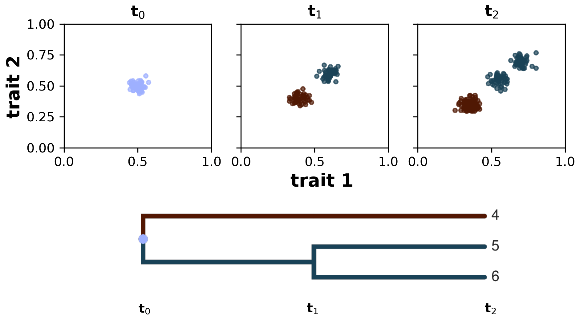
Figure 2Taxon definition implemented in AdaScape by using a spectral clustering algorithm. The algorithm groups individuals according to their common ancestry and similarity of trait values. In the three subplots we show the distribution of individuals in trait space along the axes trait 1 and trait 2 at three time steps: t0, t1, and t2. Below the subplots we show the phylogenetic reconstruction of the identified taxa, starting from the last common ancestor with a taxon ID equal to 0 all the way to taxa 4–6 at time t2.
This taxon definition is primarily based on the divergence of individuals' traits since they are the main dynamic variables affecting selection, mutation, and competition. However, the spectral clustering algorithm can be modified to accommodate other variables (e.g. geographical location of individuals or time since the last branching point). Furthermore, the taxon definition is independent of the eco-evolutionary processes of the model; thus, changing the taxon definition would not affect the model behaviour.
2.5 Landscape evolution component
The environment where organisms adapt is defined here at a landscape scale and can consider common landforms such as mountains, plateaus, stream valleys, basins, and floodplains, among others. These landforms and their evolution can be reproduced using a landscape evolution model (LEM), which in essence describes the changes in topography h by the competition of processes that shape earth's surface, such as uplift and erosion, (Whipple, 2004; Tucker and Hancock, 2010) as
where the first term U is the uplift rate (m yr−1; Table 1), the second term I is the river incision or stream power law (SPL) (Lague, 2014), and the last term accounts for hillslope processes. The river incision is the main erosional process of landforms and in simple terms describes how a flow of water cuts through bedrock and can be given by
where kf is the constant of erodability (m1−2a yr−1; Table 1), ν is precipitation rate (scaled by a reference rate), A is the drainage area (m2), and S is the slope of the terrain. The latter two enter the SPL as power functions with, respectively, exponents a and b. As the rivers cut through the valleys they create slopes that are thus subject to processes such as soil creep, landslides, and debris flows. Hence, the last term in Eq. (6) describes the transport of such material from hilltops to lowlands, also known as hillslope processes, which is determined by a constant transport coefficient or diffusivity kd (m2 yr−1; Table 1) and the curvature of the terrain (m m−2) as
Modelling fluvial incision by a stream power equation requires finding the numerical solution of a partial differential equation with linear and nonlinear slopes, which posed stability, accuracy, and speed constraints (Tucker and Hancock, 2010). However, one can overcome these issues by using FastScape (Braun and Willett, 2013), which is an efficient algorithm to compute the discharge at each node in an orderly manner following the steepest descent of the water flow to the base level in the landscape. This algorithm has been implemented in the FastScape framework (Bovy, 2021) together with various other processes affecting landforms, such as orographic precipitation (Smith and Barstad, 2004), sediment transport, and deposition by rivers (Yuan et al., 2019) among many other tectonic, climatic, and erosional processes. While elevation is the main output of the LEM, this environmental field could be used as a proxy for temperature. This would require further assumptions, for example, that temperature decreases with elevation around 6.5 ∘C km−1 (Minder et al., 2010) and a given baseline temperature at sea level, which could be constant or change over time and taken from climatic palaeo-reconstructions.
In particular, orographic precipitation is a crucial environmental process that affects the availability of water for biota and influences the surface processes briefly mentioned before. FastScape computes rainfall fields using the linear orographic precipitation model proposed by Smith and Barstad (2004), which takes into account the topography, direction, and speed of the wind to predict the spatial distribution of rainfall by solving the advection equations that integrate cloud water density and rain/snow density using a Fourier transformation into the two horizontal directions (Smith and Barstad, 2004). (Explaining the details of all the processes included in FastScape go beyond the scope of this paper, and therefore we refer the reader to the documentation of the framework and related publications, e.g. (Whipple, 2004; Smith and Barstad, 2004; Tucker and Hancock, 2010; Braun and Willett, 2013; Lague, 2014; Yuan et al., 2019; Bovy, 2021).)
We use the SPL with hillslope processes and orographic precipitation to demonstrate how the distribution and evolution of taxa respond to dynamic changes in the topography and precipitation. To model precipitation and landscape evolution, we select values of the uplift rate U, the constant of erodability kf, the transport coefficient kd, a background precipitation rate P0, wind speed ws, and wind direction wd. A description of the parameters and the values used in the examples below can be found in Table 1.
Lastly, to connect the eco-evo model with LEM, the local environmental condition zi is equal to the elevation h or the orographic precipitation ν fields as provided by FastScape at the position of the individual i at every time step. These environmental fields form the basis to compute the optimal trait value (Eq. 2) to which each individual compares to quantify its fitness (Eq. 1).
3.1 Evolutionary branching along a linear environmental gradient
Our first example considers the evolution of one trait representing the adaptation of individuals to topographic elevation, which is simply termed as “trait elevation” here. The simple eco-evolutionary model produces patterns of evolutionary branching under fewer than 500 time steps along a continuous environmental gradient. Whereas evolutionary branching is referred to here as the split of a population with an average trait value into two populations with a progressive widening gap between their average trait values, the emergence of evolutionary branching along a continuous environmental gradient is a well-known phenomenon captured in eco-evolutionary models that build on the adaptive dynamics theoretical framework (Metz et al., 1996; Geritz et al., 1998; Dieckmann et al., 2004; Klausmeier et al., 2020) and is exemplified by the seminal work of Doebeli and Dieckmann (2003).
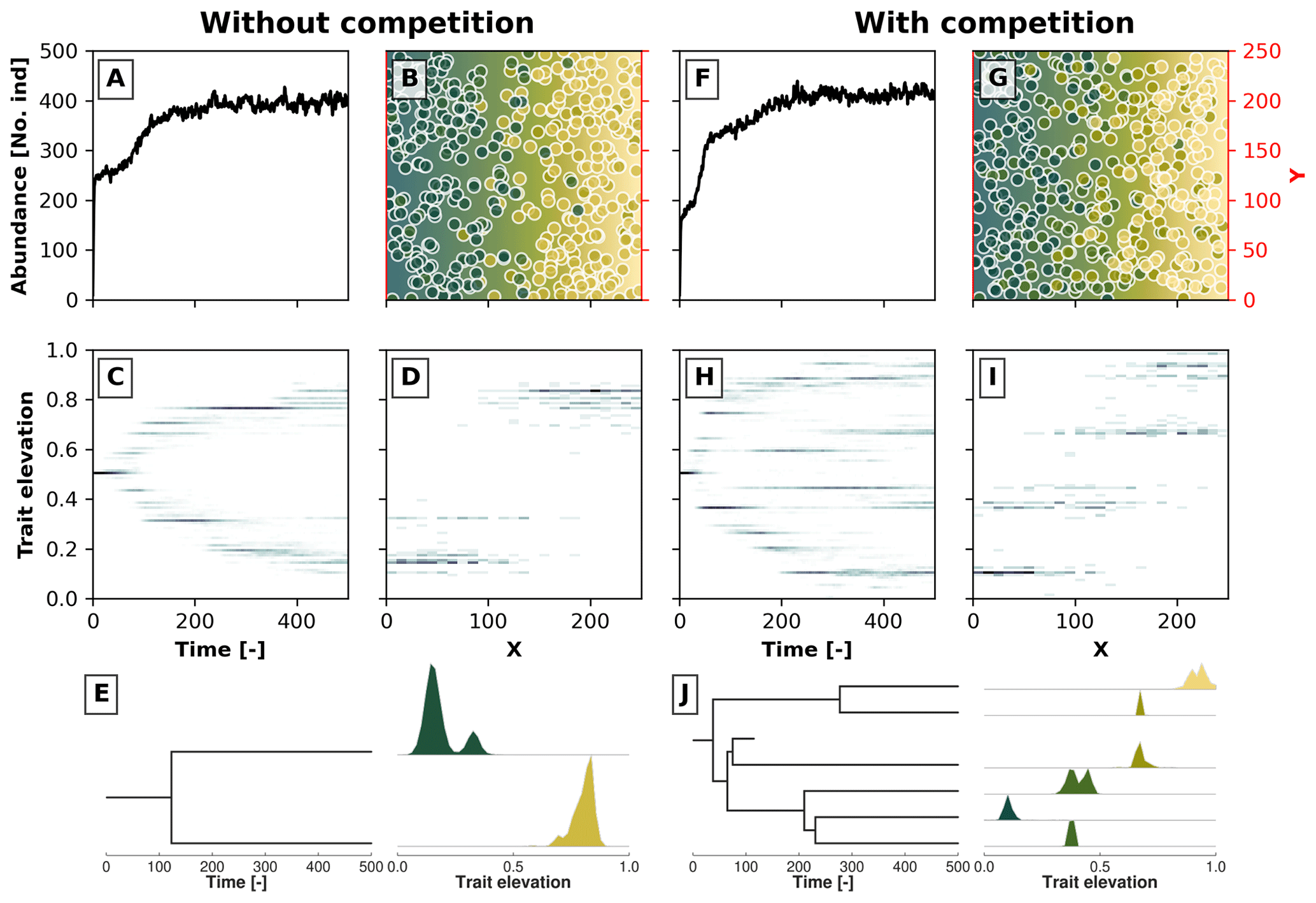
Figure 3Example simulations along a 2D gradient showing the effects trait-mediated competition has without (a–e) and with (f–j) evolutionary branching patterns. Panels (a) and (f) show the temporal changes in the number of individuals. Panels (c) and (h) show the trait distribution over time in a 2D histogram, where the darker colour marks a higher number of individuals with a given trait value at a particular time. Panels (b) and (g) show the spatial distribution of individuals in the 2D environment at the last time step, where the blue colour reflects lower trait values and the yellow colour reflects higher trait values. The coloured dots represent individuals with their corresponding trait values. Panels (d) and (i) show the distribution of trait values along the x coordinate at the last time step. In panels (e) and (j) we reconstruct the phylogenetic tree for, respectively, the simulations without and with trait-mediated competition. At each extant branch in the phylogenetic tree, we plotted the trait distribution of that particular taxon.
In Fig. 3 we show two such results for a case without trait-mediated competition (σu=2; Fig. 3a, b, c, d, and e) and with trait-mediated competition (σu=0.2; Fig. 3f, g, h, i, and j) in a simple 2D environment, where the environmental gradient (e.g. elevation) linearly increases along the x coordinate. The other parameters for these simulations are σf=0.2, μm=0.005, σm=0.05, and σd=30. We set the local carrying capacity K to 50 for the case without trait-mediated competition and K=35 for the case with trait-mediated competition. This parameterisation leads to a roughly equal saturation in the total number of individuals in the two scenarios (Fig. 3a and f) in contrast to an equal K that would predict higher individual abundances in the case of trait-mediated competition. Changes in total abundance (via changes in carrying capacity) are known to affect the number of taxa in this types of eco-evolutionary model that use a similar taxon definition (Pontarp and Wiens, 2017). Therefore, to minimise density-dependent effects on taxon richness we assure that both cases reach similar total abundances (≈400 individuals; Fig. 3a and f) by reducing local carrying capacity (but see Appendix A for a sensitivity analysis of the effects of selected parameters on the maximum abundance of individuals).
Both simulations show branching, but when competition among individuals with similar trait values is strengthened, further branching is promoted (cf. Fig. 3c and h). Figure 3b and g show the spatial distribution and Figure 3d and i show the trait distribution of the extant taxa without and with trait-mediated competition. The phylogenetic reconstruction using our proposed taxon definition (Fig. 3e and j) resembles the pattern of population trait values over time both in terms of the number of branches and the trait distributions of each branch (Fig. 3c, d, h, and i). However, this method would also separate taxa even if branches on a population level could not be distinguished (i.e. when organisms occupy all trait space). Furthermore, the taxon definition method (Sect. 2.4) can create phylogenies when organisms are described by more than one trait.
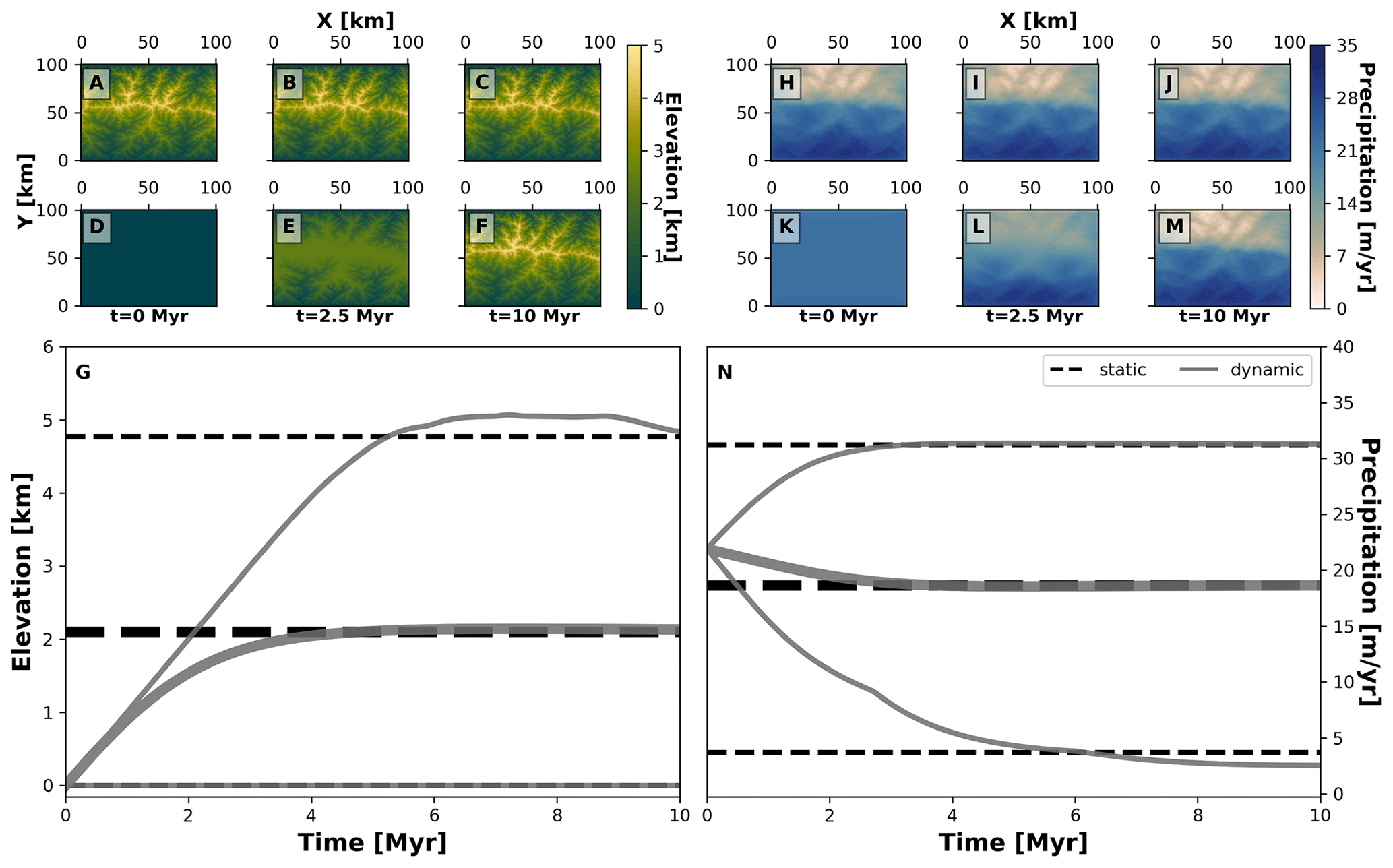
Figure 4Spatial and temporal patterns of environmental fields under static and dynamic landscape conditions. We consider two main environmental fields: elevation (a–g) and precipitation (h–n). For each one, we consider two types of environmental histories: one for a static landscape where conditions are constant (a–c, h–j, and dashed black lines in g and n) and another for a dynamic landscape for which conditions vary throughout the simulation (d–f, k–m, and solid grey curves in g and n). The thick grey curves mark the mean and the thinner grey curves are the minimum and maximum of each environmental field. To produce these environmental conditions we consider the following parameterisation of our landscape evolution model (Table 1): U=0 m yr−1 (static) or 0.001 m yr−1 (dynamic), kf=0 m1−2a yr−1 (static) or m1−2a yr−1 (dynamic), kd=0 m2 yr−1 (static) or 0.01 m2 yr−1 (dynamic). Relevant values are a=0.4, b=1, P0=22 m yr−1, ws=15 m s−1, and wd=0∘.
3.2 Biodiversity patterns in static vs. dynamic landscapes
Our second example considers the evolution of two traits representing the adaptation of species to topographic elevation and to orographic precipitation, termed here as “trait elevation” and “trait precipitation”, respectively. This experiment shows how different biodiversity patterns can emerge from the interaction of eco-evolutionary and earth surface processes using AdaScape. For this we consider two contrasting environmental histories that produce the same final mountain belt: (a) a static landscape where the topography and precipitation do not change over time (i.e. no uplift or erosional processes) and (b) a dynamic landscape where both topography and orographic precipitation change as a function of uplift over time. In Fig. 4 we show the predicted topography and precipitation for these two model setups in an idealised landscape of 100 by 100 km and for a total simulation time of about 10 Myr with time steps of 10 kyr. The resulting landform consists of a mountain belt with a main drainage divide in the middle of the model domain (Fig. 4a, b, c, d, e, and f), which reaches a maximum height of ≈5 km. This high topography creates an orographic barrier to the wind that moves in a south-to-north direction, thus producing the typical high precipitation on the windward slope of the mountain belt and a rain shadow with drier conditions on the leeward slope of the mountain belt (Fig. 4h, i, j, k, l, and m). The simulations for static and dynamic landscapes reach equivalent mean, maximum, and minimum values of elevation and precipitation (Fig. 4g and n).
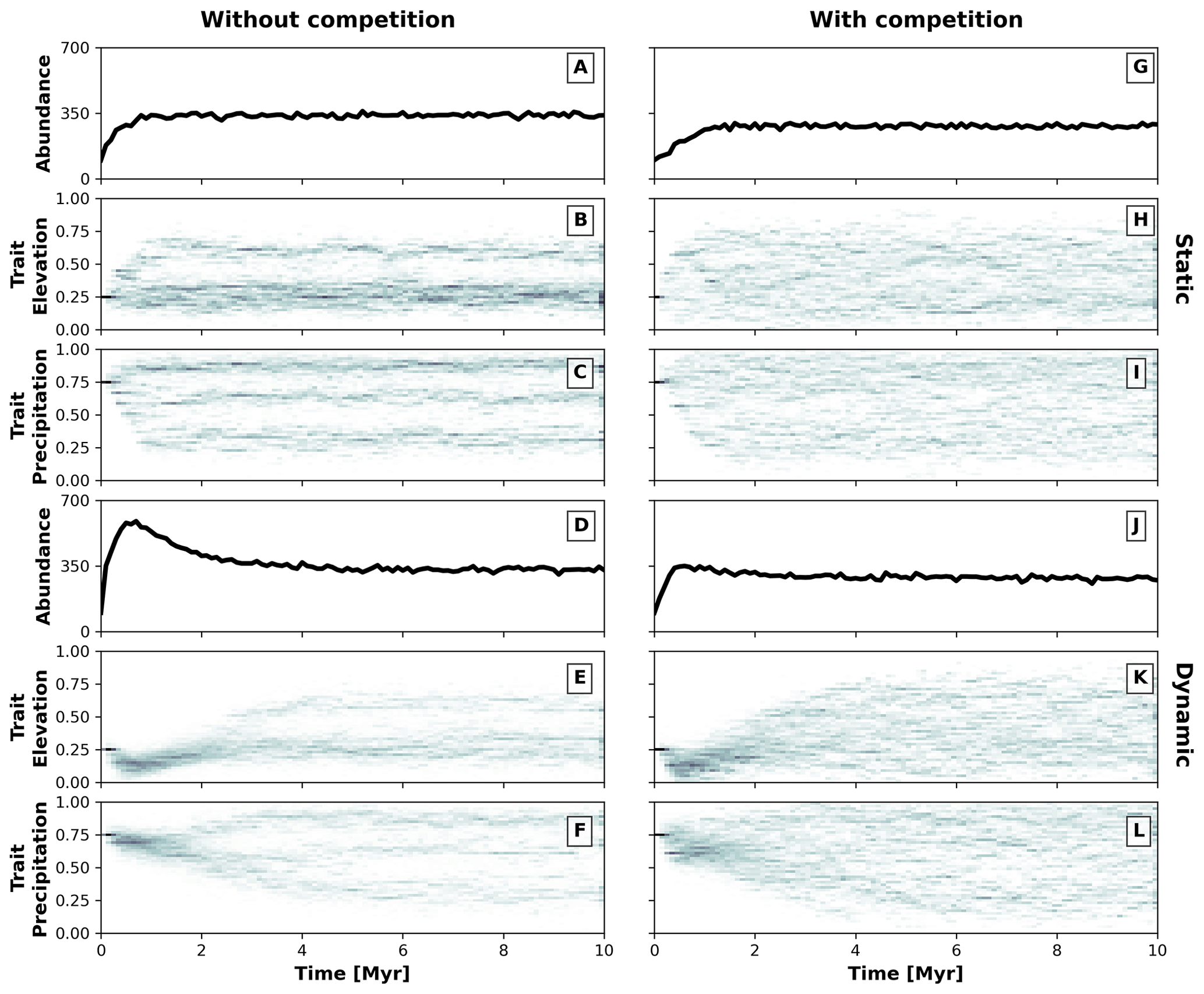
Figure 5Temporal dynamics of the eco-evolutionary model without (a–f) and with (g–l) trait-mediated competition and each for a static (a–c and g–i) and dynamic (d–f and j–l) landscape. Panels (a), (d), (g), and (j) show the number of individuals over time. Panels (b) and (c), (e) and (f), (h) and (i), and (k) and (l) present the trait distribution over time. We use 2D histograms for presenting the temporal distributions of traits (b, c, e, f, h, i, k, l), where the darker colouration highlights the higher frequency of individuals with a particular trait value.
We parameterise two eco-evolutionary models: one without (σu=2; Eq. 4) and another with (σu=0.2; Eq. 4) trait-mediated competition, which we then run in the static and dynamic landscapes (Fig. 4). We start all simulations with a monomorphic population of around 100 individuals (Fig. 5a, d, g, and j) where all individuals have similar trait values set to 0.25 for the trait associated with elevation (Fig. 5b, e, h, and k) and 0.75 for the trait associated with precipitation (Fig. 5c, f, i, and l). This represents an initial population composed of individuals adapted to lowlands and high precipitation. To avoid large differences in the fitness values of the initial populations, we set the individuals to start at specific locations either in the southern portion or at random locations in the landscape for the static or dynamic landscape conditions, respectively. We assume that the relationship between the optimal trait value and the environmental field is positive for both traits (i.e. αz=0.95; Eq. 2). The traits are considered to be independent (ρ=0; Eq. 1) and the value for the environmental fitness variability is set as a strong selection for traits around the optimal trait values (σf=0.2; Eq. 1). Mutation probability pm is set to 0.005 and mutation variability σm to 0.05, which introduces a small intergenerational trait variability. We parameterise dispersal variability, σd, to 10 km. Local carrying capacity, K (Eq. 5), is parameterised to 50 (without trait-mediated competition) and 25 (with trait-mediated competition) individuals where the radius of the local neighbourhood r is set to 20 km.
For the coupled execution of the eco-evolutionary model into the LEM we have to assume that one generation time is equal to one time step of LEM. This, of course, can lead to unrealistic generation times that exceed the average lifespan of organisms. Therefore, careful consideration of the parameters is required when AdaScape is coupled with FastScape since one generation would then represent the temporal aggregation of numerous real generations. (See Sect. 5 for a discussion on the scaling limitations.)
These two contrasting environmental conditions lead to distinct temporal patterns for simulations without and with trait-mediated competition. As the simulation progresses, the number of individuals increases until reaching similar total abundances of around 350 individuals (Fig. 5a, d, g, and j) and different diversification patterns emerge (Fig. 5b, c, e, f, h, i, k, and l), in particular, between a static (Fig. 5b, c, h, i) and dynamic (Fig. 5e, f, k, l) landscape. Under a static landscape, the evolutionary branching occurs sooner than under dynamic landscape conditions, because in the latter the individuals first are selected for narrow environmental ranges, which then extend towards the end of the simulation. The environmental conditions progressively increase during the first 2 Myr of the simulation (Fig. 4), which leads to the narrowly observed trait variability. Between 2 and 6 Myr the environmental gradients extend into broader precipitation and elevation ranges (Fig. 4) and consequently lead to an increase in trait variability. After 6 Myr the environmental fields reach their maximum extent (Fig. 4), with little trait variability until the end of the simulation (Fig. 5).
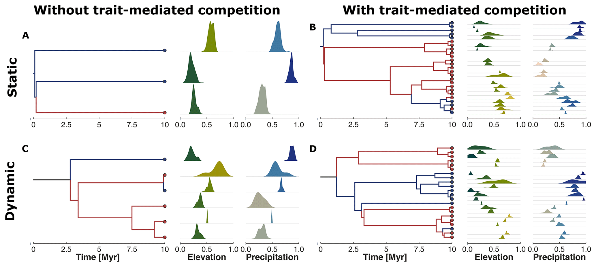
Figure 6Phylogenetic reconstruction of the extant taxa at the end of the simulation. The subplots represent our four examples without (a, c) or with (b, d) trait-mediated competition and under environmental conditions of a static (a, b) or dynamic (c, d) landscape (cf. Fig. 4). The red and blue circles in the tips of the phylogenetic trees highlight the upper half (north) and lower half (south) average location of the taxa along the y coordinate. We similarly marked the branches with the same colour coding to better distinguish the relationships between the north dry-adapted (red) and south wet-adapted (blue) clades. The density plots on the right of each tree show the trait distribution for each taxa and for traits associated with elevation and precipitation.
The reconstructed phylogenetic history for the taxa at the end of the simulation summarises the emergent diversity patterns of the four example simulations (Fig. 6). We observed that simulations without trait-mediated competition lead to lower taxon richness (i.e. three and six taxa for static and dynamic landscapes, respectively) compared with simulations with trait-mediated competition (i.e. 25 and 22 for static and dynamic landscapes, respectively). We can distinguish a division between those clades from mostly wet-adapted taxa in the south and mostly dry-adapted taxa in the north (cf. red and blue coloured lineages in Fig. 6). Such a division between the northern and the southern clades under dynamic landscape conditions (cf. Fig. 6c and d) seems to coincide with the increase in the range of the environmental gradients (Fig. 4g and n). This suggests a relationship between the rate of change in environmental conditions and the response in the build-up of biodiversity.
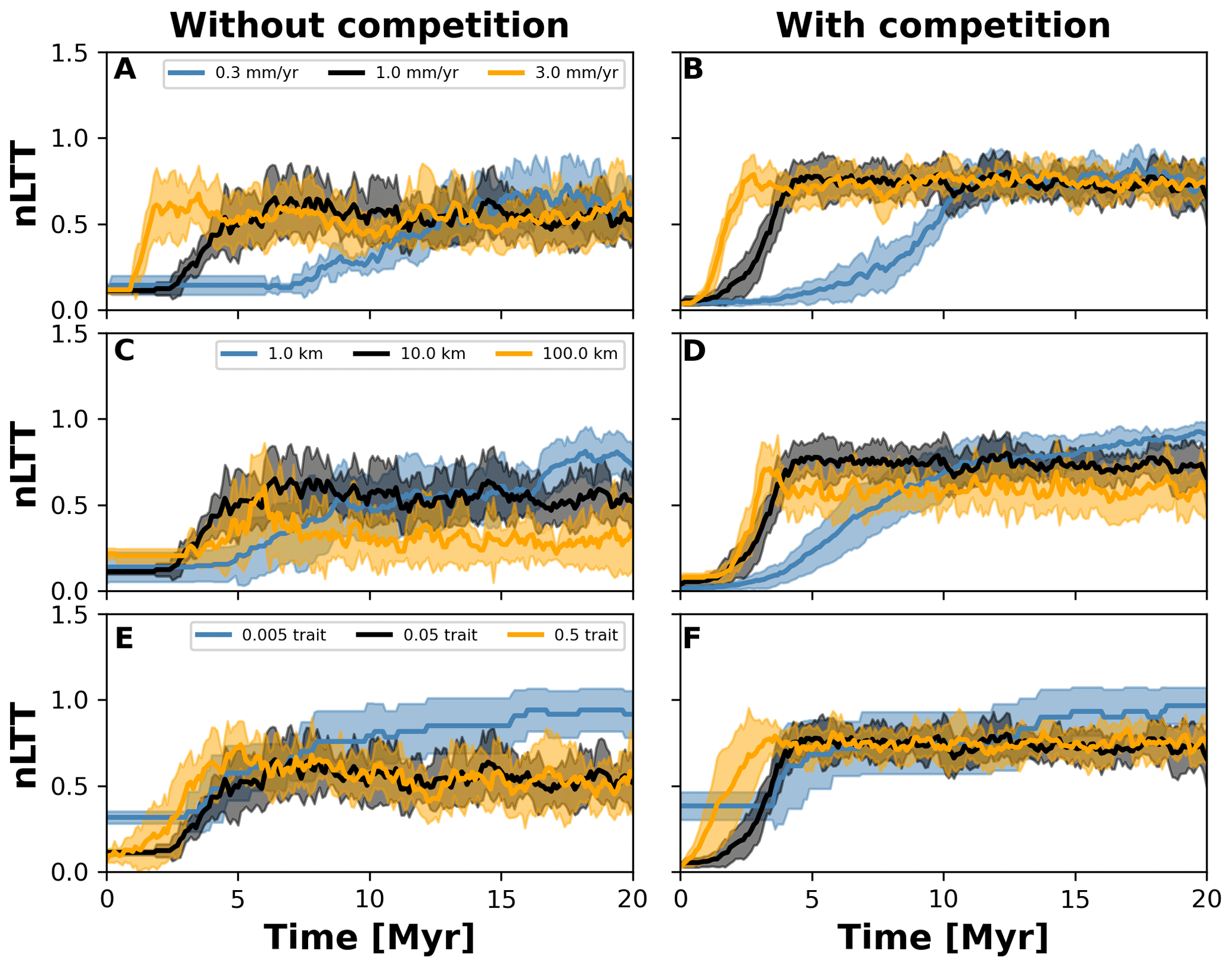
Figure 7Normalised lineages through time (nLTT) plots summarising numerical experiments where we investigate the effects of uplift rate (a, b), dispersal variability (c, d), and mutation variability (e, f). The results for each treatment are the mean (solid curves) and standard deviation (shaded areas) of 10 replicates with different random seeds. To facilitate the comparisons among treatments, we normalised the number of lineages to the maximum number that each single replicate reached. We also doubled the simulation time to 20 Myr but kept time step 10 kyr (cf. Fig. 6) to ensure that both the landscape (in the case of different uplift rates) and number of taxa would reach equilibrium.
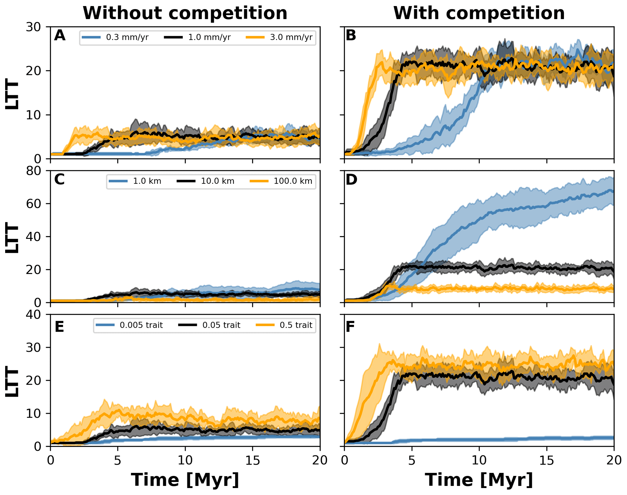
Figure 8Number lineages through time (LTT) plots summarising numerical experiments where we investigated the effects of uplift rate (a, b), dispersal variability (c, d), and mutation variability (e–f). The results for each treatment are the mean (solid curves) and standard deviation (shaded areas) of 10 replicates with different random seeds. Results are based on the same observations in Fig. 7.
3.3 Effects of uplift, mutation, and dispersal variability on biodiversity
To investigate how the build-up of biodiversity is influenced by the rate of change in environmental conditions and eco-evolutionary processes, we varied three parameters, namely uplift rate, dispersal variability, and mutation variability (Table 1). In Figs. 7 and 8, we quantified how these changes affect the number of lineages through time (LTT), in particular when taxon biodiversity reaches its maximum. For the two competition cases, we tested three different values of uplift, dispersal, and mutation centred around the parameterisation used in the example in Sect. 3.2 (Figs. 5 and 6; Table 1). For each parameter set, we repeated the simulation 10 times for a total of 60 simulations. In Fig. 7, we normalised each LTT by the maximum number of lineages reached on each simulation.
We observed that as the mountain is uplifted faster, the maximum number of lineages is reached earlier (Fig. 7a and b). Conversely, the peak in the number of lineages is delayed as the rate of uplift slows (Fig. 7a and b). Changes in uplift rate similarly affect simulations with and without trait-mediated competition (cf. Fig. 7a and b, respectively). However, in absolute terms, the simulations with trait-mediated competition lead to a higher number of lineages (Fig. 8), while the overall patterns remain similar to the normalised values (Fig. 7).
The eco-evolutionary processes also show differences in the timing with respect to the values tested and between cases of competition. On the one hand, a low dispersal variability leads to a slower build-up of diversity compared with intermediate and higher values (Fig. 7c and d). However, as time progresses the intermediate and high dispersal cases tend to reach their maximum earlier, while the simulations with low dispersal values continue to increase (Fig. 7c and d). This is reflected in the highest number of lineages, in absolute terms, reached for the low dispersal with trait-mediated competition cases (Fig. 8c and d). On the other hand, increasing mutation variability causes a faster build-up of diversity, while the contrary occurs when the values of mutation variability decrease (Fig. 7e and f). In absolute terms, an increase in mutation variability tends to increase the number of lineages, with the highest values predicted with trait-mediated competition cases (Fig. 8e and f).
Our eco-evolutionary implementation is built on the model proposed by Irwin (2012), who showed how a phylogeographic structure (i.e. an historical geographic distribution of clades) emerges along an environmental gradient as selection, dispersal, mutation, and population size vary. Irwin's model is similar to earlier eco-evolutionary models, such as that of Doebeli and Dieckmann (2003), which described adaptive speciation patterns (or evolutionary branching of a trait) along environmental gradients. Doebeli and Dieckmann (2003) showed the range of parameters where branching is facilitated and the importance of ecological processes. Particularly, they demonstrated that when competition strength is smaller than the selection strength, branching is promoted (Doebeli and Dieckmann, 2003). Albeit in Irwin's original model, competition for resources was not considered, we show here that including such ecological process facilitates speciation (Figs. 2 and 6). Both works also show how an increase in dispersal leads to well-mixed and spatially unstructured populations (Doebeli and Dieckmann, 2003; Irwin, 2012), which will thus dampen the number of lineages – a pattern we also identified with our model (Figs. 7 and 8).
Contemporary to Irwin's work, Pontarp et al. (2012) proposed an eco-evolutionary model also inspired by Doebeli and Dieckmann (2003) but using a different fitness generating function and reconstructing taxa and phylogenies based on the similarity of trait values and shared common ancestry. The latter has helped Pontarp et al. (2012) to extend the traditional application of these types of eco-evolutionary models from population to community. They have used this model to show how (a) phylogenetic structure emerges in communities competing for resources (Pontarp et al., 2012), (b) mode of speciation (from sympatric to allopatric) can change continuously (even during a single radiation event) depending on local to regional conditions and dispersal capacity of organisms (Pontarp et al., 2015), and (c) richness patterns along gradients depend on the carrying capacity, diversification rates, and time for speciation (Pontarp and Wiens, 2017). We have adopted a similar approach to that of Pontarp and colleagues to define taxa, which allows us to broaden the applicability of the model and reconstruct idealised phylogenies that can be compared with time-calibrated phylogenies.
Another characteristic of the works of Irwin (2012) and Pontarp et al. (2012) is that they divide the environmental gradient into discrete habitats, while Doebeli and Dieckmann (2003) use a spatially continuous and linear environmental gradient. Haller et al. (2013), building on the work of Doebeli and Dieckmann (2003), tested the effects that various spatially complex environments (i.e. linear gradients, nonlinear gradients, and spatially continuous patches) have on branching. They found that an intermediate level of environmental heterogeneity promotes branching, and they suggested using metrics of their realised environments to compare with observations in real landscapes. In addition, Doebeli and Dieckmann (2003) demonstrated, early on, the impact of the relationship between the slope of the environmental gradient with dispersal by revealing that evolutionary branching is facilitated at intermediate environmental gradients once dispersal is below a critical level. Here by coupling our adaptive speciation model to a landscape evolution model, we not only produce a more realistic landscape but also show the impact of considering an environmental gradient that changes over time (i.e. a dynamic landscape).
A recent tool named the gen3sis engine can simulate ecological and evolutionary processes in palaeo-geographies that are changed at discrete time-steps (Hagen et al., 2021a). This tool was used to investigate the effects that plate tectonics and palaeo-climate reconstructions have on macroecological patterns of diversity, such as the latitudinal diversity gradient (Hagen et al., 2021a), and pantropical diversity disparity (Hagen et al., 2021b). This engine offers a great wealth of outcomes (e.g. species distributions, phylogeny, and ecological traits) that can seamlessly be compared with empirical observations. Other similar models that mainly focused on the ecological and evolutionary aspects have been proposed earlier (Rangel et al., 2018) in what is known as “population-based spatially explicit mechanistic eco-evolutionary models” (MEEMs) (Hagen, 2022). Our model differs from MEEMs in that we follow an individual-based (IBM) or agent-based (ABM) modelling approach, which in comparison to population-based models offers greater flexibility into the processes considered and how the organisms interact among themselves and with the environment (Levin, 1998; Railsback, 2001; DeAngelis and Mooij, 20005; Grimm et al., 2005). IBMs thus account for low-level variability that can be scaled up to higher hierarchical levels, producing emergent properties that cannot be predicted by the properties of individuals or their interactions with the environment alone (Levin, 1998; Railsback, 2001; DeAngelis and Mooij, 20005; Grimm et al., 2005). Nevertheless, accounting for individual-level variability, particularly as observed in nature, can be impractical and computationally demanding. Hence, population-based models, such as MEEMs, are a more computationally efficient option (Hagen, 2022). In addition, MEEMs, such as those in Rangel et al. (2018) and Hagen et al. (2021a), do not compute the landscape dynamics but instead use a priori calculated environmental fields. This approach allows them a more flexible and efficient way to upscale the computations. However, this comes at the cost of not controlling the relevant processes that lead to the building of a landform or climate as in our coupled eco-evolutionary and landscape evolution model.
Recent efforts to couple eco-evolutionary models with an LEM, such as BioSlant (Stokes and Perron, 2020), present a more promising venue to explore the link between tectonics, climate, and biodiversity. However, Stokes and Perron (2020) implemented a different eco-evolutionary model that captures mainly allopatric speciation. Their model is based on an earlier version of a neutral metapopulation model (Muneepeerakul et al., 2007) where speciation is not linked to functional traits and the organisms only move along river networks. Hence, a species or taxon in this type of model is a static definition. Since mobility is limited to river networks, the main application is to investigate the effects of river reorganisation on biodiversity. Our approach circumvents these limitations through the continuous interplay between organisms' traits and their environment.
Any model at its best is a surrogate of nature that we can use to test our understanding of a system. We decided to build on established theoretical frameworks to study the coupled eco-evolutionary dynamics (Metz et al., 1996; Geritz et al., 1998; Dieckmann et al., 2004; McGill and Brown, 2007; Klausmeier et al., 2020) and landscape evolution (Whipple, 2004; Tucker and Hancock, 2010; Lague, 2014). As these theoretical frameworks have had many applications over the past decades with more detailed descriptions of processes as we have shown here, we use only their essential processes to illustrate how bio- and geo-components of the earth system can be coupled into a single modelling framework while keeping the number of parameters and processes to a minimum. While it is appealing to integrate ecological and evolutional processes into a landscape evolution model, several caveats related to the scaling of such processes need to be taken into consideration. Three types of scaling problems are recognised in ecological models, namely pre-model (i.e. (dis)aggregation of values used as input of models), in-model (i.e. procedures related to the simplification of a model), and post-model (i.e. scaling procedures applied to the output of models) issues (Fritsch et al., 2020). Here we focus on the pre-model and in-model scaling issues, particularly those related to maintaining computational efficiency while keeping the ability to detect emergent speciation patterns (Fritsch et al., 2020).
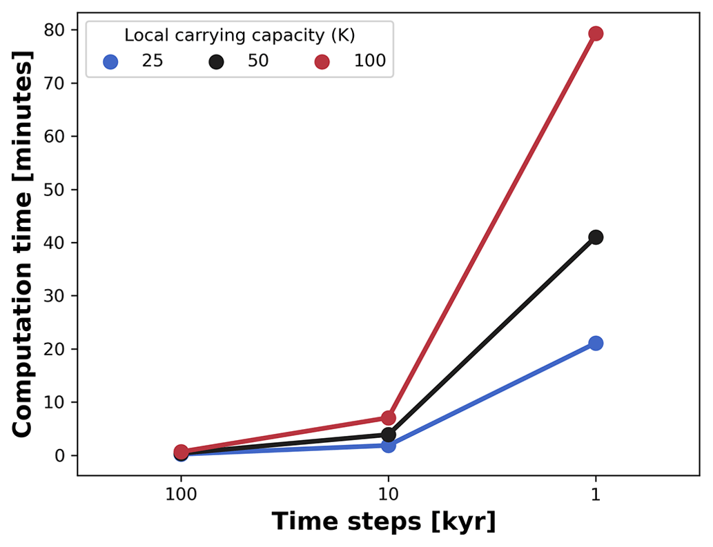
Figure 9Average computation time for a single AdaScape run. We measured the average time variation between seven runs set up without trait-mediated competition as shown in examples (cf. Figs. 5 and 6). We then manipulated the local carrying capacity and the length of the time steps in the model. For all simulations, the spatial extent consists of an area of 100 by 100 km, which is divided in a regular grid of 100 by 100 points. The simulations are executed for 10 Myr with variable time steps in a 176-core (Intel Xeon 2.10 GHz) Linux cluster.
Coupling these types of models comes at the expense of increased computational cost. To prevent this, we developed our simple eco-evolutionary model on a very efficient algorithm to solve the stream power law (Braun and Willett, 2013) and its implementation using xarray-simlab infrastructure (Bovy et al., 2021). This implementation, known as FastScape, provides a series of libraries to efficiently compute and parallelise simulations (Bovy, 2021). Hence, our model executes on the order of minutes with computational costs exponentially increasing as the number of time steps and the maximum number of individuals (local carrying capacity) increases (Fig. 9). For all simulations, the spatial extent consists of an area of 100 by 100 km, which is divided in a regular grid of 100 by 100 points. The simulations were executed for 10 Myr with variable time steps, as explained in Fig. 9. Although we run these simulations in a 176-core (Intel Xeon 2.10 GHz) Linux cluster, the execution of FastScape and AdaScape do not require any high-performance computing facilities and can be executed on any modern desktop or laptop computer where Python can be installed with similar performance as shown in Fig. 9.
When AdaScape is coupled with FastScape, the time between generations is defined as the time step of the LEM (i.e. 10 kyr for the example simulations shown in Sect. 3.2). Therefore, a generation in AdaScape would represent the temporal aggregation of numerous real generations. In this context, a scaling of the eco-evolutionary parameters related to mutation (pm, σm) and dispersal (σd) must be considered. The simplest way is to scale the mutation and dispersal parameters by the square root of the number of real generations in an LEM time step. Therefore, the parameter p used in a given simulation with a time step Δt should be scaled for comparison with measured values p′ by the following relationship: , where tG is the average lifespan of a generation, p is one of the mutation or dispersal parameters, and p′ is the new scaled parameter. Caveats of this scaling are that the parameter value is not directly constrained by observations and that, obviously, this parameter should not be too large in a simulation to avoid, for example, that dispersal exceed the length of the simulated area or that all individuals mutate and vary the trait value broadly in a single time step. Particularly, the latter goes back to the assumptions of earlier formulations of adaptive dynamics stating that the range of validity of these types of eco-evolutionary models remains intact as long as mutation processes were rare and the trait variability with respect to their ancestor was small, to assure that evolutionary dynamics were slower than changes in population densities (Abrams, 2001; Klausmeier et al., 2020).
In addition, keeping a tractable number of individuals during the simulations can be a challenge. Further developments can use scaling-up procedures, for example, the so-called super-individuals approach (Scheffer et al., 1995), to be able to represent even higher abundances of individuals. This would require limiting the number of individuals to a predefined maximum and minimum number, where each of these super individuals accounts for the properties of several others.
Competition for resources is an important ecological process (Tilman, 1982; Chesson, 2000) that can lead to the divergence of traits and consequently promote biodiversity (Pfennig and Pfennig, 2009). Examples of both interspecific (e.g. Grant and Grant, 2006; Grainger et al., 2021) and intraspecific (e.g. Bolnick, 2001; Calsbeek and Cox, 2010) competition are known to leave an imprint on the traits under selection. Therefore, ecological processes have the potential to alter the outcome of evolution. Increasing interest in the past decades has been in documenting cases where ecological dynamics and evolutionary dynamics show reciprocal interactions (Fussmann et al., 2007; Schoener, 2011; Govaert et al., 2019), thus leading to a recurring call to integrate the distinct disciplines of ecology and evolution, as recently pointed out by Loreau et al. (2023). This becomes particularly relevant knowing that both ecological and evolutionary dynamics can operate at the same pace (Fussmann et al., 2007; Schoener, 2011; Govaert et al., 2019) and can be influenced by rapid changes in the environment, for example, as the climate changes (Parmesan, 2006; Loreau et al., 2023); hence, the difficulty in understanding the tangled relationships between the biotic and abiotic environment with the ecological and evolutionary responses of organisms. Our model, although aiming at capturing the essential eco-evolutionary processes, simplifies much of the organism–organism and organism–environment feedback. Nevertheless, the results support the general view that competition is an important process that promotes the build-up of taxon diversity.
There is a great appeal for numerical tools that look to integrate various components of the earth system such as tectonics, climate, and biodiversity, although such tools are not common (Antonelli et al., 2018). Some of the existing tools focus on the eco-evolutionary components, leaving behind earth's surface processes and climate, while others do not factor in eco-evolutionary dynamics and trait–environment relationships. Here we introduce our coupling of a simple eco-evolutionary model into a very efficient landscape evolution model, FastScape, which offers great potential to explore the links between the three main components of the earth system into a single modelling framework and at manageable computational costs. This allows us, as we show here, to perform a large number of simulations and consider ensemble properties rather than those emerging from single simulations, the details of which can be highly dependent on the initial conditions or the stochastic nature of the evolution equations representing mutation and dispersal. At the moment, AdaScape mainly considers the effect that the environment has on the biota; however, feedback between these components can be further investigated. For example, organisms such as plants are known to affect the hydrological cycle by dampening the discharge variability of rivers (Rossi et al., 2016). Plants can thus impact the erosional efficiency of rivers where erosional thresholds exist (Deal et al., 2018; Braun and Deal, 2023). This would require us to investigate and test relationships between organismal traits with erosional processes in the landscape, which offer a potential venue to further integrate various components of the earth system into a single modelling framework.
Due to stochastic and nonlinear relationships of the processes, as well as our definition of the local neighbourhood in the eco-evolutionary model, it is difficult to know a priori how the different processes will interact to produce a maximum number of individuals. Therefore, we performed a sensitivity analysis on the maximum number of individuals Nmax to changes in the parameters σf, σu, and σd in relation to changes in radius r and local carrying capacity K. We then tested 10 values for the ranges of , σu=[0.2, 2], and in relation to changes in 10 values in the range of and . We performed 100 simulations for each pair-wise set of parameters for a total of 700 simulations (Fig. A1). We observed that the maximum number of individuals will be reached as r decreases and K increases; also, the maximum number of individuals when K increases and σu and σd decrease or when σf increases. Similarly, the highest Nmax is reached when σu and σd decrease or when σf increases, in combination with a decrease in the radius of the local neighbourhood r.
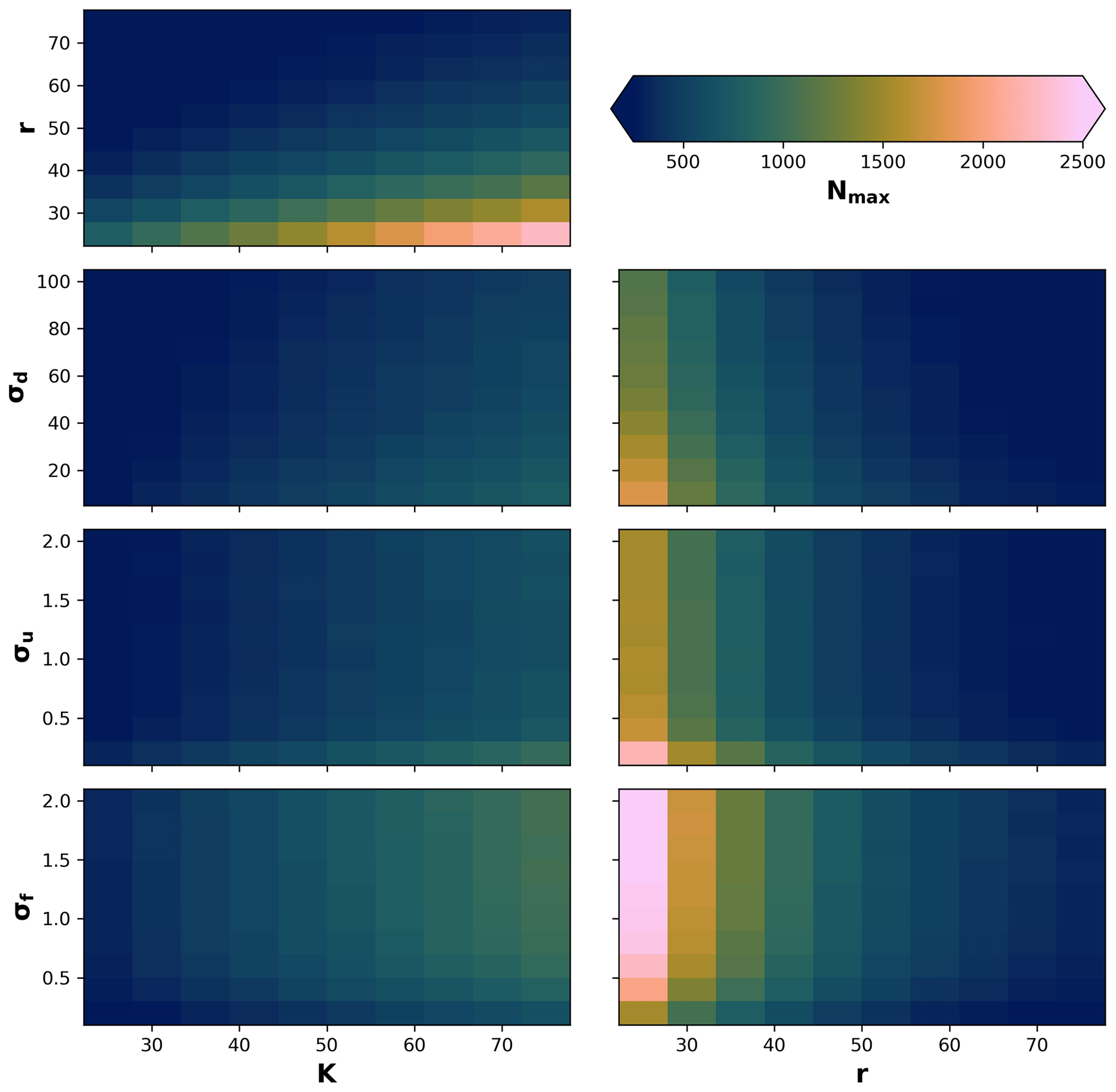
Figure A1The maximum number of individuals (Nmax) reached during a simulation given a set of parameters. The model results are calculated using the Sect. 3.1 setup for a linear environmental gradient. The default parameter values are r=30, K=50, σf=0.2, σu=2, and σd=30.
The effects of competition in our model depend on the relationship between the environmental field and optimal trait, as well as on the heterogeneity in the environment. To better illustrate this, in Fig. B1 we performed a model run as in Sect 3.1 for the case with competition (σu), where we set the environment–optimal trait relationship (α) from the default value 0.95 to 0, the latter meaning that there is no relationship between the trait and the environmental field. We then ran this model setup under an environment with a linear environmental gradient (as in Fig. 3) and under no environmental gradient, i.e. a constant environmental field centred at a middle elevation. We observed no build-up of taxon diversity when there was no environment–optimal trait relationship (α=0) without (Fig. B1a, b, c, and d) and with (Fig. B1e, f, g, and h) a linear environmental gradient, and when α>0 with a linear environmental gradient (Fig. B1i, j, k, and l). Trait-mediated competition thus only promotes diversity when a trait environmental relationship exists and when the simulation occurs in a heterogeneous environment (as in Fig. 3f, g, h, i, and j).
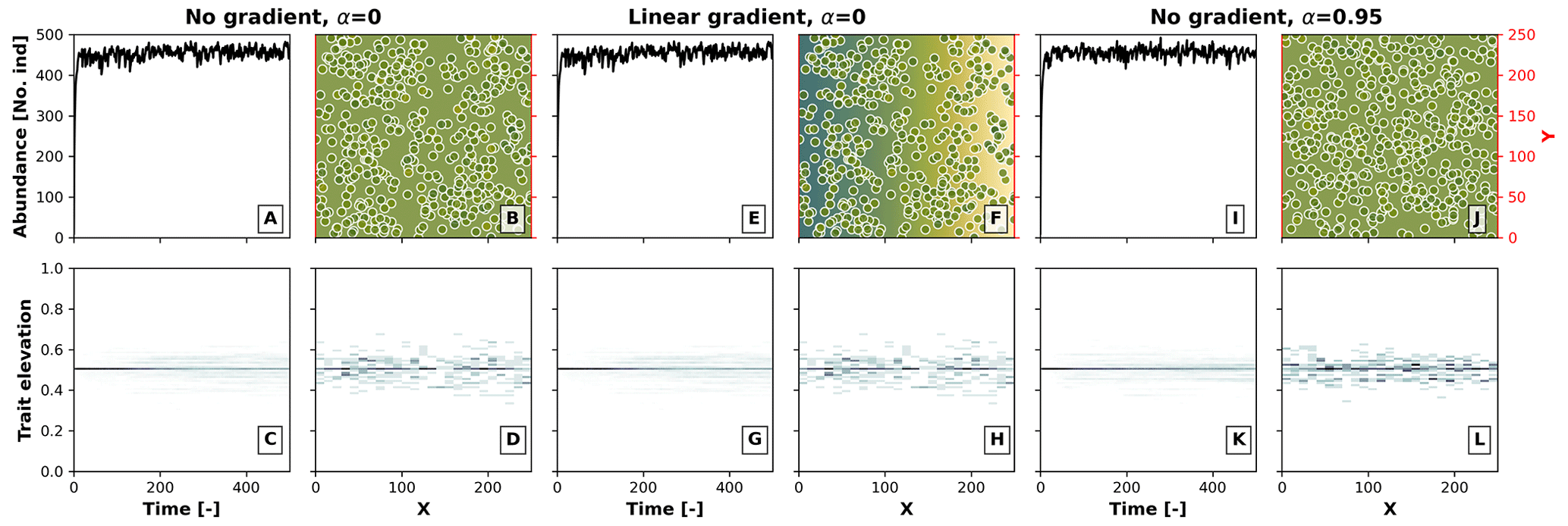
Figure B1Effects of the environment–optimal trait relationship (α) and competition on the build-up of taxon diversity. The numerical experiments show the results of simulations with (1) no environmental gradient (same elevation throughout the landscape) and no environment–trait relationship α (a–d), (2) a linear environmental gradient (as in Fig. 3) and no environment–trait relationship (e–h), and (3) no environmental gradient and a positive environment–trait relationship (α=0.95). The other parameter values are set as in Fig. 3 for the case with the trait-mediated competition.
All routines of AdaScape and FastScape are openly accessible via GitHub (https://github.com/fastscape-lem/adascape, last access: 28 November 2023) and Zenodo (https://doi.org/10.5281/zenodo.7794374; Acevedo-Trejos and Bovy, 2023). We include also the procedures to reproduce all the results presented here.
EAT extended and developed the eco-evo model, performed numerical simulations and analysis, and wrote the first draft. JB contributed to the conceptualisation of the model, the development and implementation of the algorithm, as well as the design of the numerical experiments. KK developed and tested the initial eco-evolutionary models and consulted on the extended model development. NAR helped to implement the eco-evo model. BB consulted on the extended model development and contributed to the implementation of the algorithm into FastScape. All authors provided manuscript edits and approved the final version.
The contact author has declared that none of the authors has any competing interests.
Publisher's note: Copernicus Publications remains neutral with regard to jurisdictional claims made in the text, published maps, institutional affiliations, or any other geographical representation in this paper. While Copernicus Publications makes every effort to include appropriate place names, the final responsibility lies with the authors.
We thank the German Research Foundation (DFG) that financed Esteban Acevedo-Trejos and Jean Braun via Collaborative Research Centre 1211 “Earth evolution at the dry limit” (project no. 268236062) and N. Alexia Raharinirina under Germany's Excellence Strategy – The Berlin Mathematics Research Center MATH+ (EXC-2046).
This research has been supported by the Deutsche Forschungsgemeinschaft (grant nos. 268236062 (CRC 1211) and MATH+ (EXC-2046)).
The article processing charges for this open-access publication were covered by the Helmholtz Centre Potsdam – GFZ German Research Centre for Geosciences.
This paper was edited by Andrew Wickert and reviewed by two anonymous referees.
Abrams, P.: Modelling the adaptive dynamics of traits involved in inter- and intraspecific interactions: An assessment of three methods, Ecol. Lett., 4, 166–175, https://doi.org/10.1046/j.1461-0248.2001.00199.x, 2001. a
Acevedo-Trejos, E. and Bovy, B.: fastscape-lem/adascape: First release (v1.0.0), Zenodo [code], https://doi.org/10.5281/zenodo.7794374, 2023. a
Antonelli, A., Kissling, W. D., Flantua, S. G. A., Bermúdez, M. A., Mulch, A., Muellner-Riehl, A. N., Kreft, H., Linder, H. P., Badgley, C., Fjeldså, J., Fritz, S. A., Rahbek, C., Herman, F., Hooghiemstra, H., and Hoorn, C.: Geological and climatic influences on mountain biodiversity, Nat. Geosci., 11, 718–725, https://doi.org/10.1038/s41561-018-0236-z, 2018. a, b, c
Badgley, C., Smiley, T. M., Terry, R., Davis, E. B., DeSantis, L. R. G., Fox, D. L., Hopkins, S. S. B., Jezkova, T., Matocq, M. D., Matzke, N., McGuire, J. L., Mulch, A., Riddle, B. R., Roth, V. L., Samuels, J. X., Strömberg, C. A. E., and Yanites, B. J.: Biodiversity and Topographic Complexity: Modern and Geohistorical Perspectives, Trends Ecol. Evol., 32, 211–226, https://doi.org/10.1016/j.tree.2016.12.010, 2017. a
Böhnert, T., Luebert, F., Ritter, B., Merklinger, F. F., Stoll, A., Schneider, J. V., Quandt, D., Weigend, M.: Origin and diversification of Cristaria (Malvaceae) parallel Andean orogeny and onset of hyperaridity in the Atacama Desert, Glob. Planet. Change, 181, 102992, https://doi.org/10.1016/j.gloplacha.2019.102992, 2019. a
Bolnick, D. I.: Intraspecific competition favours niche width expansion in Drosophila melanogaster, Nature, 410, 463–466, https://doi.org/10.1038/35068555, 2001. a
Boschman, L. M. and Condamine, F. L.: Mountain radiations are not only rapid and recent: Ancient diversification of South American frog and lizard families related to Paleogene Andean orogeny and Cenozoic climate variations, Glob. Planet. Change, 208, 103704, https://doi.org/10.1016/j.gloplacha.2021.103704, 2022. a
Bovy, B.: fastscape-lem/fastscape: Release v0.1.0beta3 (0.1.0beta3), Zenodo [code], https://doi.org/10.5281/zenodo.4435110, 2021. a, b, c, d
Bovy, B., McBain, G. D., Gailleton, B. and Lange, R.: benbovy/xarray-simlab: 0.5.0 (0.5.0), Zenodo [code], https://doi.org/10.5281/zenodo.4469813, 2021. a
Brännström, Å., Johansson, J., Loeuille, N., Kristensen, N., Troost, T. A., Lambers, R. H. R., and Dieckmann, U.: Modelling the ecology and evolution of communities: A review of past achievements, current efforts, and future promises, Evol. Ecol. Res., 14, 601–625, 2012. a
Braun, J. and Deal, E.: Implicit algorithm for threshold stream power incision model, J. Geophys. Res.-Earth Surf., 128, 1–32, https://doi.org/10.1029/2023JF007140, 2023. a
Braun, J. and Willett, S. D.: A very efficient O(n), implicit and parallel method to solve the stream power equation governing fluvial incision and landscape evolution, Geomorphology, 180–181, 170–179, https://doi.org/10.1016/j.geomorph.2012.10.008, 2013. a, b, c
Bromham, L.: An introduction to molecular evolution and phylogenetics, Second Edition, Oxford University Press, Oxford, UK, 536 pp., ISBN 9780198736363, 2016. a
Brown, J. H. and Maurer, B.: Macroecology: the division of food and space among species on continents, Science, 243, 1145–1150, https://doi.org/10.1126/science.243.4895.1145, 1989. a
Cabral, J. S., Valente, L., and Hartig, F.: Mechanistic simulation models in macroecology and biogeography: state-of-art and prospects, Ecography, 40, 267–280, https://doi.org/10.1111/ecog.02480, 2017. a
Calsbeek, R. and Cox, R. M.: Experimentally assessing the relative importance of predation and competition as agents of selection, Nature, 465, 613–616, https://doi.org/10.1038/nature09020, 2010. a
Cassemiro, F. A. S., Albert, J. S., Antonelli, A., Menegotto, A., Wüest, R. O., Cerezer, F., Coelho, M. T. P., Reis, R. E., Tan, M., Tagliacollo, V., Bailly, D., da Silva, V. F. B., Frota, A., da Graça, W. J., Ré, R., Ramos, T., Oliveira, A. G., Dias, M. S., Colwell, R. K., Rangel, T. F., and Graham, C. H.: Landscape dynamics and diversification of the megadiverse South American freshwater fish fauna, P. Natl. Acad. Sci. USA, 120, e2211974120, https://doi.org/10.1073/pnas.2211974120, 2023. a
Chesson, P.: Mechanisms of maintenance of species diversity, Annu. Rev. Ecol. Syst., 31, 343–358, https://doi.org/10.1146/annurev.ecolsys.31.1.343, 2000. a
Condamine, F. L., Rolland, J., and Morlon, H.: Macroevolutionary perspectives to environmental change, Ecol. Lett., 16, 72–85, https://doi.org/10.1111/ele.12062, 2013. a
Connolly, S. R., Keith, S. A., Colwell, R. K., and Rahbek, C.: Process, mechanism, and modeling in macroecology, Trends Ecol. Evol., 32, 835–844, https://doi.org/10.1016/j.tree.2017.08.011, 2017. a
Couvreur, T. L. P., Dauby, G., Blach-Overgaard, A., Deblauwe, V., Dessein, S., Droissart, V., Hardy, O. J., Harris, D. J., Janssens, S. B., Ley, A. C., Mackinder, B. A., Sonké, B., Sosef, M. S. M., Stévart, T., Svenning, J., Wieringa, J. J., Faye, A. Missoup, A. D., Tolley, K. A., Nicolas, V., Ntie, S., Fluteau, F., Robin, C., Guillocheau, F., Barboni, D., and Sepulchre, P.: Tectonics, climate and the diversification of the tropical African terrestrial flora and fauna, Biol. Rev., 96, 16–51, https://doi.org/10.1111/brv.12644, 2021. a
Deal, E., Braun, J., and Botter, G.: Understanding the role of rainfall and hydrology in determining fluvial erosion efficiency, J. Geophys. Res.-Earth Surf., 123, 744–778, https://doi.org/10.1002/2017JF004393, 2018. a
DeAngelis, D. L. and Mooij, W. M.: Individual-based modeling of ecological and evolutionary processes, Annu. Rev. Ecol. Evol. Syst., 36, 147–168, https://doi.org/10.1146/annurev.ecolsys.36.102003.152644, 2005. a, b
Dieckmann, U., Doebeli, M., Metz, J. A. J., and Tautz, D.: Adaptive speciation, Cambridge University Press, Cambridge, UK, https://doi.org/10.1017/CBO9781139342179, 2004. a, b, c
Dieckmann, U., Brännström, Å., HilleRisLambers, R., and Ito, H. C.: The adaptive dynamics of community structure, in Mathematics for Ecology and Environmental Sciences, Springer, Berlin, Germany, 145–177, https://doi.org/10.1007/978-3-540-34428-5_8, 2007. a
Ding, W. N., Ree, R. H., Spicer, R. A., and Xing, Y. W.: Ancient orogenic and monsoon-driven assembly of the world's richest temperate alpine flora, Science, 369, 578–581, https://doi.org/10.1126/science.abb4484, 2020. a
Doebeli, M. and Dieckmann, U.: Speciation along environmental gradients, Nature, 421, 259–264, https://doi.org/10.1038/nature01274, 2003. a, b, c, d, e, f, g, h, i, j, k
Fjeldså, J., Bowie, R. C. K., and Rahbek, C.: The role of mountain ranges in the diversification of birds, Annu. Rev. Ecol. Evol. Syst., 43, 249–265, https://doi.org/10.1146/annurev-ecolsys-102710-145113, 2012. a
Fritsch, M., Lischke, H., and Meyer, K. M.: Scaling methods in ecological modelling, Methods Ecol. Evol., 11, 1368–1378, https://doi.org/10.1111/2041-210X.13466, 2020. a, b
Fussmann, G. F., Loreau, M., and Abrams, P. A.: Eco-evolutionary dynamics of communities and ecosystems, Funct. Ecol., 21, 465–477, https://doi.org/10.1111/j.1365-2435.2007.01275.x, 2007. a, b
Geritz, S. S. A. H., Kisdi, É., Meszéna, G., and Metz, J. A. J.: Evolutionarily singular strategies and the adaptive growth and branching of the evolutionary tree, Evol. Ecol., 12, 35–57, https://doi.org/10.1023/A:1006554906681, 1998. a, b, c
Gotelli, N. J., Anderson, M. J., Arita, H. T., Chao, A., Colwell, R. K., Connolly, S. R., Currie, D. J., Dunn, R. R., Graves, G. R., Green, J. L., Grytnes, J., Jiang, Y., Jetz, W., Lyons, S. K., McCain, C. M., Magurran, A. E., Rahbek, C., Rangel, T. F., Soberón, J., Webb, C. O., and Willig, M. R.: Patterns and causes of species richness: A general simulation model for macroecology, Ecol. Lett., 12, 873–886, https://doi.org/10.1111/j.1461-0248.2009.01353.x, 2009. a
Govaert, L., Fronhofer, E. A., Lion, S., Eizaguirre, C., Bonte, D., Egas, M., Hendry, A. P., De Brito Martins, A., Melián, C. J., Raeymaekers, J. A. M., Ratikainen, I. I., Saether, B., Schweitzer, J. A., and Matthews, B.: Eco-evolutionary feedbacks – Theoretical models and perspectives, Funct. Ecol., 33, 13–30, https://doi.org/10.1111/1365-2435.13241, 2019. a, b
Grainger, T. N., Rudman, S. M., Schmidt, P., and Levine, J. M.: Competitive history shapes rapid evolution in a seasonal climate, P. Natl. Acad. Sci. USA, 118, e2015772118, https://doi.org/10.1073/pnas.2015772118, 2021. a
Grant, P. R. and Grant, B. R.: Evolution of character displacement in Darwin’s finches, Science, 313, 224–226, https://doi.org/10.1126/science.1128374, 2006. a
Grimm, V., Revilla, E., Berger, U., Jeltsch, F., Mooij, W. M., Railsback, S. F., Thulke, H., Weiner, J., Wiegand, T., and DeAngelis, D. L.: Pattern-oriented modeling of agent-based complex systems: Lessons from ecology, Science, 310, 987–991, https://doi.org/10.1126/science.1116681, 2005. a, b, c
Hagen, O., Flück, B., Fopp, F., Cabral, J. S., Hartig, F., Pontarp, M., Rangel, T. F., and Pellissier, L.: gen3sis: A general engine for eco-evolutionary simulations of the processes that shape Earth's biodiversity, PLoS Biol., 19, e3001340, https://doi.org/10.1371/journal.pbio.3001340, 2021a. a, b, c, d, e
Hagen, O., Skeels, A., Onstein, R. E., Jetz, W., and Pellissier, L.: Earth history events shaped the evolution of uneven biodiversity across tropical moist forests, P. Natl. Acad. Sci. USA, 118, e2026347118, https://doi.org/10.1073/pnas.2026347118, 2021b. a
Hagen, O.: Coupling eco-evolutionary mechanisms with deep-time environmental dynamics to understand biodiversity patterns, Ecography, 2023, 1–16, https://doi.org/10.1111/ecog.06132, 2022. a, b, c
Haller, B. C., Mazzucco, R., and Dieckmann, U.: Evolutionary branching in complex landscapes, Am. Nat., 182, 127–141, https://doi.org/10.1086/671907, 2013. a
Hoorn, C., Wesselingh, F. P., ter Steege, H., Bermudez, M. A., Mora, A., Sevink, J., Sanmartín, I., Sanchez-Meseguer, A., Anderson, C. L., Figueiredo, J. P., Jaramillo, C., Riff, D., Negri, F. R., Hooghiemstra, H., Lundberg, J., Stadler, T., Särkinen, T., and Antonelli, A.: Amazonia through time: andean uplift, climate change, landscape evolution, and biodiversity, Science, 330, 927–931, https://doi.org/10.1126/science.1194585, 2010. a
Irwin, D. E.: Local adaptation along smooth ecological gradients causes phylogeographic breaks and phenotypic clustering, Am. Nat., 180, 35–49, https://doi.org/10.1086/666002, 2012. a, b, c, d, e, f, g, h
Klausmeier, C. A., Kremer, C. T., and Koffel, T.: Trait-based ecological and eco-evolutionary theory, in Theoretical Ecology: concepts and applications, edited by: McCann, K. S., and Gellner, G., Oxford University Press, Oxford, UK, https://doi.org/10.1093/oso/9780198824282.003.0011, 2020. a, b, c, d
Lague, D.: The stream power river incision model: Evidence, theory and beyond, Earth Surf. Process. Landforms, 39, 38–61, https://doi.org/10.1002/esp.3462, 2014. a, b, c
Lenton, T. M., Schellnhuber, H. J., and Szathmáry, E.: Climbing the co-evolution ladder, Nature, 431, 913, https://doi.org/10.1038/431913a, 2004. a
Levin, S. A.: Ecosystems and the biosphere as complex adaptive systems, Ecosystems, 1, 431–436, https://doi.org/10.1007/s100219900037, 1998. a, b
Loreau, M., Jarne, P., and Martiny, J. B. H.: Opportunities to advance the synthesis of ecology and evolution, Ecol. Lett., 1–5, https://doi.org/10.1111/ele.14175, 2023. a, b
Lynch, M. Evolution of the mutation rate, Trends Genet., 2, 345–352, https://doi.org/10.1016/j.tig.2010.05.003, 2010. a
Martínez, C., Jaramillo, C., Correa-Metrío, A., Crepet, W., Moreno, J. E., Aliaga, A., Moreno, F., Ibañez-Mejia, M., and Bush, M. B.: Neogene precipitation, vegetation, and elevation history of the central andean plateau, Sci. Adv., 6, 1–10, https://doi.org/10.1126/sciadv.aaz4724, 2020. a
McGill, B. J. The what, how, and why of doing macroecology, Glob. Ecol. Biogeogr., 28, 6–17, https://doi.org/10.1111/geb.12855, 2019. a
McGill, B. J. and Brown, J. S.: Evolutionary game theory and adaptive dynamics of continuous traits, Annu. Rev. Ecol. Evol. Syst., 38, 403–435, https://doi.org/10.1146/annurev.ecolsys.36.091704.175517, 2007. a, b
McGill, B. J., Enquist, B. J., Weiher, E., and Westoby, M.: Rebuilding community ecology from functional traits, Trends Ecol. Evol., 21, 178–185, https://doi.org/10.1016/j.tree.2006.02.002, 2006. a
Metz, J. A. J., Geritz, S. A H., Meszéna, G., Jacobs, F. J. A., and van Heerwaarden, J. S. Adaptive Dynamics : A Geometrical Study of the Consequences of Nearly Faithful Reproduction, in: Stochastic and spatial structures of dynamical systems, edited by: van Strien, S. J. and Verduyn Lunel, S. M., Amsterdam, KNAW Verhandelingen, Afd. Natuurkunde, Eerste reeks, vol 45, the Netherlands, 183–231, 1996. a, b, c
Minder, J. R., Mote, P. W., and Lundquist, J. D.: Surface temperature lapse rates over complex terrain: Lessons from the Cascade mountains, J. Geophys. Res.-Atmos., 115, 1–13, https://doi.org/10.1029/2009JD013493, 2010. a
Muneepeerakul, R., Weitz, J. S., Levin, S. A., Rinaldo, A., and Rodríguez-Iturbe, I.: A neutral metapopulation model of biodiversity in river networks, J. Theor. Biol., 245, 351–363, https://doi.org/10.1016/j.jtbi.2006.10.005, 2007. a
Parmesan, C.: Ecological and evolutionary responses to recent climate change, Annu. Rev. Ecol. Evol. Syst., 37, 637–669, https://doi.org/10.1146/annurev.ecolsys.37.091305.110100, 2006. a
Pérez-Escobar, O. A., Zizka, A., Bermúdez, M. A., Meseguer, A. S., Condamine, F. L., Hoorn, C., Hooghiemstra, H., Pu, Y., Bogarín, D., Boschman, L. M., Pennington, R. T., Antonelli, A., and Chomicki, G.: The Andes through time: evolution and distribution of Andean floras, Trends Plant Sci., 27, 364–378, https://doi.org/10.1016/j.tplants.2021.09.010, 2022. a
Pfennig, K. S. and Pfennig, D. W.: Character displacement: ecological and reproductive responses to a common evolutionary problem, Q. Rev. Biol., 84, 253–276, https://doi.org/10.1086/605079, 2009. a
Pontarp, M. and Wiens, J. J.: The origin of species richness patterns along environmental gradients: uniting explanations based on time, diversification rate and carrying capacity, J. Biogeogr., 44, 722–735, https://doi.org/10.1111/jbi.12896, 2017. a, b
Pontarp, M., Ripa, J., and Lundberg, P.: On the origin of phylogenetic structure in competitive metacommunities, Evol. Ecol. Res., 14, 269–284, 2012. a, b, c, d, e
Pontarp, M., Ripa, J., and Lundberg, P.: The biogeography of adaptive radiations and the geographic overlap of sister species, Am. Nat., 186, 565–581, https://doi.org/10.1086/683260, 2015. a
Rahbek, C., Borregaard, M. K., Antonelli, A., Colwell, R. K., Holt, B. G., Nogues-Bravo, D., Rasmussen, C. M. Ø., Richardson, K., Rosing, M. T., Whittaker, R. J., and Fjeldså, J.: Building mountain biodiversity: Geological and evolutionary processes, Science, 365, 1114–1119, https://doi.org/10.1126/science.aax0151, 2019a. a, b
Rahbek, C., Borregaard, M. K., Colwell, R. K., Dalsgaard, B., Holt, B. G., Morueta-Holme, N., Nogues-Bravo, D., Whittaker, R. J., and Fjeldså, J.: Humboldt's enigma: What causes global patterns of mountain biodiversity?, Science, 365, 1108–1113, https://doi.org/10.1126/science.aax0149, 2019b. a
Railsback, S. F.: Concepts from complex adaptive systems for individual-based models, Ecol. Modell., 139, 47–62, 2001. a, b
Rangel, T. F., Edwards, N. R., Holden, P. B., Diniz-Filho, J. A. F., Gosling, W. D., Coelho, M. T. P., Cassemiro, F. A. S., Rahbek, C., and Colwell, R. K.: Modeling the ecology and evolution of biodiversity: Biogeographical cradles, museums, and graves, Science, 361, eaar5452, https://doi.org/10.1126/science.aar5452, 2018. a, b, c, d
Rossi, M. W., Whipple, K. X., and Vivoni, E. R.: Precipitation and evapotranspiration controls on daily runoff variability in the contiguous United States and Puerto Rico, J. Geophys. Res.-Earth Surf., 121, 128–145, https://doi.org/10.1002/2015JF003446, 2016. a
Scheffer, M., Baveco, J. M., DeAngelis, D. L., Rose, K. A., and van Nes, E. H.: Super-individuals a simple solution for modelling large populations on an individual basis, Ecol. Modell., 80, 161–170, https://doi.org/10.1016/0304-3800(94)00055-M, 1995. a
Schoener, T. W.: The newest synthesis: Understanding the interplay of evolutionary and ecological dynamics, Science, 331, 426–429, https://doi.org/10.1126/science.1193954, 2011. a, b
Smith, R. B. and Barstad, I.: A linear theory of orographic precipitation, J. Atmos. Sci., 61, 1377–1391, https://doi.org/10.1175/1520-0469(2004)061<1377:ALTOOP>2.0.CO;2, 2004. a, b, c, d
Spicer, R. A.: Tibet, the Himalaya, Asian monsoons and biodiversity - In what ways are they related?, Plant Divers., 39, 233–244, https://doi.org/10.1016/j.pld.2017.09.001, 2017. a
Stokes, M. F. and Perron, J. T.: Modeling the evolution of aquatic organisms in dynamic river basins, J. Geophys. Res.-Earth Surf., 125, 1–19, https://doi.org/10.1029/2020JF005652, 2020. a, b
Tilman, D.: Resource competition and community structure, Princeton University Press, Princeton, New Jersey, United States of America, ISBN 9780691083025, 1982. a
Tucker, G. E. and Hancock, G. R.: Modelling landscape evolution, Earth Surf. Process. Landforms, 35, 28–50, https://doi.org/10.1002/esp.1952, 2010. a, b, c, d, e
Viles, H.: Biogeomorphology: Past, present and future, Geomorphology, 366, 106809, https://doi.org/10.1016/j.geomorph.2019.06.022, 2020. a, b
Violle, C., Reich, P. B., Pacala, S. W., Enquist, B. J., and Kattge, J.: The emergence and promise of functional biogeography, P. Natl. Acad. Sci. USA, 111, 13690–13696, https://doi.org/10.1073/pnas.1415442111, 2014. a
von Luxburg, U.: A tutorial on spectral clustering, Stat. Comput., 17, 395–416, https://doi.org/10.1007/s11222-007-9033-z, 2007. a
Webb, C. T., Hoeting, J. A., Ames, G. M., Pyne, M. I., and LeRoy Poff, N.: A structured and dynamic framework to advance traits-based theory and prediction in ecology, Ecol. Lett., 13, 267–283, https://doi.org/10.1111/j.1461-0248.2010.01444.x, 2010. a
Whipple, K. X.: Bedrock rivers and the geomorphology of active orogens, Annu. Rev. Earth Planet. Sci., 32, 151–185, https://doi.org/10.1146/annurev.earth.32.101802.120356, 2004. a, b, c
Wiens, J. J. and Donoghue, M. J.: Historical biogeography, ecology and species richness, Trends Ecol. Evol., 19, 639–644, https://doi.org/10.1016/j.tree.2004.09.011, 2004. a
Yuan, X. P., Braun, J., Guerit, L., Simon, B., Bovy, B., Rouby, D., Robin, C., and Jiao, R.: Linking continental erosion to marine sediment transport and deposition: A new implicit and O(N) method for inverse analysis, Earth Planet. Sci. Lett., 524, 115728, https://doi.org/10.1016/j.epsl.2019.115728, 2019. a, b
- Abstract
- Introduction
- Model description
- Examples
- Comparison with similar modelling approaches
- Limitations of our modelling approach
- Competition as a driver of diversity
- Conclusions
- Appendix A: Sensitivity on the maximum number of individuals to changes in selected parameters
- Appendix B: Trait-mediated competition, optimal trait–environment relationship, and environmental heterogeneity
- Code and data availability
- Author contributions
- Competing interests
- Disclaimer
- Acknowledgements
- Financial support
- Review statement
- References