Peatland-VU-NUCOM (PVN 1.0): using dynamic plant functional types to model peatland vegetation, CH₄, and CO₂ emissions

Despite covering only 3 % of the planet’s land surface, peatlands store 30 % of the planet’s terrestrial carbon. The net greenhouse gas (GHG) emissions from peatlands depend on many factors but primarily soil temperature, vegetation composition, water level and drainage, and land management. However, many peatland models rely on water levels to estimate CH₄ exchange, neglecting to consider the role of CH₄ transported to the atmosphere by vegetation. To assess the impact of vegetation on the GHG fluxes of peatlands, we have developed a new model, Peatland-VU-NUCOM (PVN). The PVN model is a site-specific peatland CH₄ and CO₂ emissions model, able to reproduce vegetation dynamics. To represent dynamic vegetation, we have introduced plant functional types and competition, adapted from the NUCOM-BOG model, into the framework of the Peatland-VU model, a peatland GHG emissions model. The new PVN model includes plant competition, CH₄ diffusion, ebullition, root, shoot, litter, exudate production, belowground decomposition, and aboveground moss development under changing water levels and climatic conditions.

Here, we present the PVN model structure and explore the model's sensitivity to environmental input data and the introduction of the new vegetation competition schemes. We evaluate the model against observed chamber data collected at two peatland sites in the Netherlands to show that the model is able to reproduce realistic plant biomass fractions and daily CH₄ and CO₂ fluxes. We find that daily air temperature, water level, harvest frequency and height, and vegetation composition drive CH₄ and CO₂ emissions. We find that this process-based model is suitable to be used to simulate peatland vegetation dynamics and CH₄ and CO₂ emissions.

1 Introduction

Despite covering only 3 % of the planet’s land surface, peatlands store 30 % (644 GtC) of the planet’s terrestrial carbon (Yu et al., 2010). The present-day global radiative effect of peatlands on the climate is estimated to be between −0.2 and −0.5 W m⁻² (i.e. a net cooling) (Frolking and Roulet, 2007) in comparison to a radiative forcing of +2.43 Wm⁻² due to anthropogenic greenhouse gas (GHG) emissions since pre-industrial times (WGI, 2021). Future changes to the climate will impact the carbon sequestration capacity of peatlands; however, the net effect of climate change on peatlands is not yet understood (Loisel et al., 2021). Research indicates that some peatlands will form a positive feedback (Dorrepaal et al., 2009), whilst others will form a neutral (Saleska et al., 2002) or negative feedback to warming of the global climate system (Melillo et al., 2002; Lafleur et al., 2003), and the net effect of these complex responses is not yet known. The net warming effect of peatlands on the global climate system, and particularly the potential to both emit and drawdown CO₂ and CH₄, means that peatlands have a complex and multifaceted relationship with the global climate system.

The net GHG emissions from peatlands depends on many factors but primarily vegetation composition, land management, ground water level and drainage, and soil temperature (Dorrepaal et al., 2009; Tiemeyer et al., 2016). Rewetting drained peatlands is one strategy proposed to combat enhanced CO₂ emissions from peatlands, but this has been documented to both enhance and reduce GHG emissions (e.g. Günther et al., 2020; Boonman et al., 2022) with the majority of studies concluding that rewetting leads to enhanced CH₄ and net GHG emissions (Harpenslager et al., 2015; Knox et al., 2015). Field studies have shown that vegetation restoration in combination with rewetting may reduce GHG emissions (Graf and Rochefort, 2009; Mazzola et al., 2022). Vegetation impacts the net GHG emissions in peatlands by directly influencing the net primary production and organic matter available for decomposition and indirectly and by influencing the substrates available for microbial metabolisation in the soil column (Bansal et al., 2020; Bridgham et al., 2013).

While the effects of the groundwater table on peatland GHG emissions are extensively described (Evans et al., 2021), the impacts of plant type and plant community composition on GHG emissions are less understood (Malmer et al., 2003). Changes in vegetation composition have been observed in long-running water table manipulation experiments (Peltoniemi et al., 2009; Strack et al., 2006). Generally, sedges and mosses establish during wetter conditions, and shrubs and trees develop during drier conditions, with enhanced Sphagnum growth outcompeting shrubs during warming experiments (Dorrepaal et al., 2006). Belowground, changes in vegetation have been accompanied by changes in bacterial and fungal biomass (Jaatinen et al., 2008) and methanogenic and methanotrophic community diversity (Yrjälä et al., 2011; Lippmann et al., 2021). Changes to CO₂ (NPP) have been observed following changes in plant community composition, further impacting root exudation (Ballantyne et al., 2014). Root exudates are a diverse group of organic compounds secreted by plant roots into the nearby soil. The composition and quality of root exudates varies between plant types, influencing microbial community composition and function and CO₂ (Crow and Wieder, 2005) and CH₄ fluxes (Schipper and Reddy, 1996). Plant growth, root exudation, and decomposition of organic matter happen at rates that differ depending on plant type (Dorrepaal et al., 2007). Sphagnum is a primary contributor to the carbon sequestration in many peatlands and decomposes 3 times slower than most vascular plants (Graf and Rochefort, 2009). Spatial variation in the rate of vegetation growth and decomposition, particularly for bryophyte species, leads to the creation of microforms, such as hummocks, hollows, and lawns, which, in turn, impact the water level relative to the surface and spatially variable fluxes (Waddington and Roulet, 2000). Differences in vegetation composition within the same site and with the same water levels have been observed to lead to differences in CH₄ fluxes (Bubier, 2016; Jackowicz-Korczyński et al., 2010). To understand the role of vegetation emissions' feedbacks during peatland restoration efforts, vegetation must thus be treated as a dynamic interactive element of the peatland ecosystem.

Plants with common ecosystem functions or structures can be represented with common model algorithms or parameters in a vegetation model when grouped as plant functional types (PFTs) (Wullschleger et al., 2014). Plant functional types have been found to explain uncertainties in GHG emissions from wetlands in response to warming in a meta-analysis of wetlands exposed to warming (Bao et al., 2023). Dynamic (rather than static) PFTs simulate the inter-seasonal growing and dying of plants that, over a number of years, lead to vegetation succession and are critical to reliably assess the impacts of climate and environmental change on peatland ecosystems (Box et al., 2019). Shifts in community composition lead to feedbacks between species and other environmental parameters such as soil moisture, bulk density, soil organic matter (SOM) content, gas conduit function, rate of growth, rate of decomposition, microbial mineralisation, and aerobic decomposition (De Boeck et al., 2011). Dynamic plant representation is critical to reliably simulate vegetation–environmental feedbacks in models (Toet et al., 2006); therefore, the inclusion of dynamic vegetation classes is critical to reliably estimate C, CO₂, and CH₄ emissions from peatlands during periods of environmental change (Li et al., 2016; Laine et al., 2022).

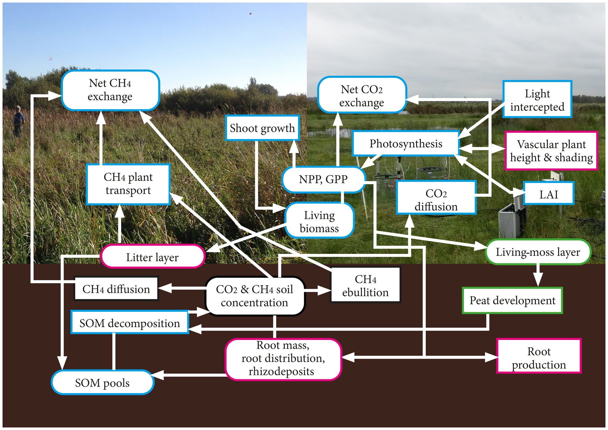
Figure 1 Schematic of the movement of carbon in the model. Processes are delineated with rectangles, whereas carbon pools are delineated with curved edges. The pink outline represents non-moss pools and processes, the green outline represents pools and processes applicable only to moss PFTs, and the blue outline refers to pools and processes that are applicable to all plant types. In the background of this figure, the Horstermeer site is shown on the left, and the Ilperveld site is shown on the right.

Many peatland carbon cycle models have been developed over the preceding decades. The Wetland and Wetland CH₄ Inter-comparison of Models Project (WETCHIMP) evaluated the ability of a variety of models to simulate large-scale wetland characteristics and corresponding CH₄ emissions (Melton et al., 2013; Wania et al., 2013). Peatland modelling efforts have made significant advancements to simulate CH₄ fluxes by including CH₄-specific processes such as CH₄ plant transport and ebullition. However, many models rely on CO₂ fluxes or surface water levels as indicators of CH₄ exchange (Metzger et al., 2015), restricting their capacity to assess feedbacks between environmental change and the peatland CH₄ cycle. There exist two pre-existing models that simulate dynamic vegetation, CO₂, and CH₄ cycling in peatlands (i.e. PEATBOG (Wu et al., 2016) and LPJ-WHyMe (Wania et al., 2010)), thereby limiting the ability of the modelling community to assess model mechanistic processes. The functionality and scope of current models that simulate peatlands and include either dynamic or static vegetation are compared in Table S1 in the Supplement. The PEATBOG model simulates three PFTs – moss, shrubs, and graminoids – at the Mer Bleue bog site and represents a comprehensive array of peatland processes, including the nitrogen cycle and dissolved gases (carbon, CO₂, and CH₄). LPJ-WHyMe, like its parent model, LPJ-WHy (Sitch et al., 2003; Gerten et al., 2004), includes permafrost and peatlands, two peatland-specific PFTs (flood-tolerant C₃ graminoids and Sphagnum mosses), a new decomposition scheme when under inundation, and the addition of root exudates. LPJ-WHyMe particularly assesses the impacts of inundation on vegetation composition, net primary production, and the deceleration of decomposition under inundation.

To assess the impact of dynamic vegetation classes on subsequent GHG fluxes in peatlands, we present a new model, Peatland-VU-NUCOM v1.0 (PVN). PVN incorporates features of NUCOM-BOG, a bog ecosystem model (Heijmans and Berendse, 2008), into the Peatland-VU model framework, a process-based peatland model (van Huissteden et al., 2006). The NUCOM-BOG model simulates vegetation competition and C, nutrient, and water cycling in undisturbed bog ecosystems under changing climates using a soil profile divided by an acrotelm–catotelm boundary where plant growth and decomposition are partitioned between plant organs. The Peatland-VU model simulates the CH₄ and CO₂ cycle within a column of peat soil with varying water levels. The Peatland-VU model simulates CH₄ fluxes, gross primary productivity, and CO₂ cycle whilst assuming a constant plant layer, and it does not include a nitrogen cycle. We have developed a model that, with the appropriate site input data, can be used to simulate peatland sites with a wide variety of vegetation types and vegetation management practices. For this reason, there is no limit to the number of PFTs that can be included in a model simulation. The inclusion of dynamic vegetation classes into the PVN model provides a model that is capable of estimating the greenhouse gas balance in response to environmental changes (changes in temperature, radiation, precipitation or evapotranspiration, or water levels) and also different management efforts (changes in harvest regime or vegetation restoration) for peatland sites. The incorporation of features of NUCOM-BOG, a model simulating undisturbed systems, into PVN, a new model simulating disturbed and managed systems, requires that changing environmental conditions and changing management practices both lead to dynamic impacts on vegetation classes. Therefore, this model can serve wetland management by estimating changes in the greenhouse gas balance of peatland sites in response to management decisions whilst considering the effects of environmental change.

2 Materials and methods

2.1 The PVN model

The new PVN model describes the vegetation, CH₄, and CO₂ dynamics of a column of an above- and belowground peatland ecosystem (Fig. 1). Carbon dioxide and CH₄ emissions enter the atmosphere by ebullition, transport through plants, diffusion through the soil, and respiration. The aboveground carbon pools are the aboveground living biomass, litter layer (non-moss PFTs only), shoots, and living-moss depth (moss PFTs only). The belowground carbon pools are the peat, labile organic matter, microbial biomass, litter and dead roots, and root exudates (Table S2).

Plant functional types (PFT) are the key element of NUCOM that is added to the Peatland-VU framework to create the PVN model. Any number of PFTs can be included in a model simulation. PFT attributes (parameters) describe plant physiology and bioclimatic limits. Bioclimatic limits are used by the photosynthesis function (Sect. 2.1.1) and the potential growth function (Eq. 13). Each PFT is defined as being either a moss or vascular plant type, which impacts the ability of plants to grow vertically or to develop roots. Each PFT is prescribed as having either evergreen or deciduous phenology. For deciduous vegetation, leaf senescence increases when the daily temperature falls below the PFT's minimum tolerated temperature, whereas, for evergreen vegetation, leaf senescence refers to the death of old leaves (Eq. 9). Maximum leaf coverage is maintained as long as the daily water level and temperature are within the ideal range. The PFT parameters are defined in Table 1, and the references are listed in Table S3. In this section, the subscript p is used to show that the equation or variable is PFT specific, z is used to indicate that the equation or variable is soil layer specific, t is used to represent time, T represents temperature, and WL represents water level. The convention used in this paper is such that a positive flux represents the movement of gas from the ecosystem to the atmosphere.

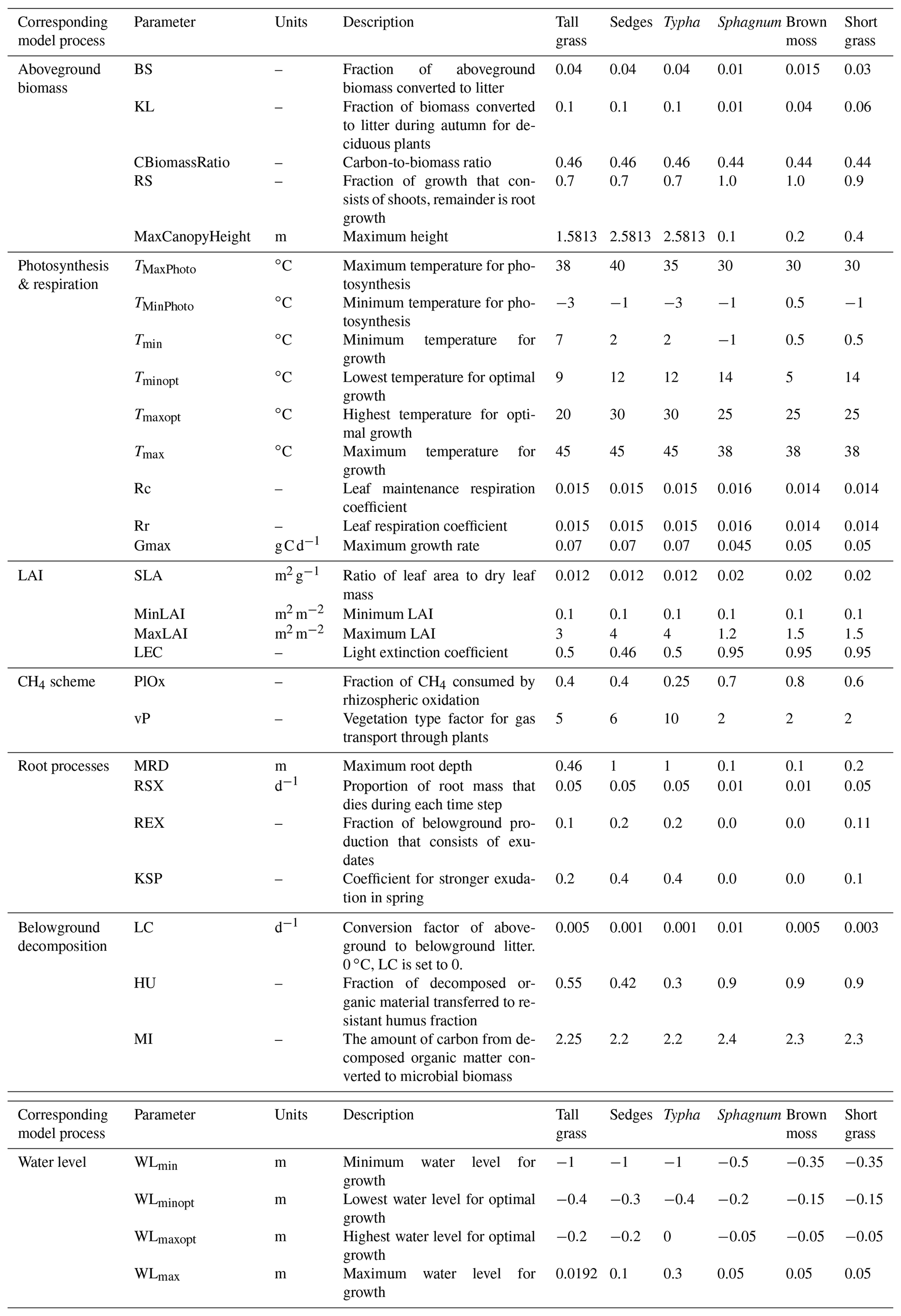
Table 1 Name, units, description, and values of PFT input parameters. Associated references are listed in Table S3. In the left column, each PFT parameter is tied to its relevant model mechanism. Note that some PFT parameters are, at times, used by multiple model processes.

2.1.1 Primary production

C3 photosynthesis, leaf respiration (RT), and net primary production (NPP) are calculated using a modified version of the primary production scheme introduced into the Peatland-VU model by Mi et al. (2014), modified from the BIOME3 equilibrium biosphere model Haxeltine and Prentice (1996). The BIOME3 model is based on the premise that GPP and leaf respiration increase with the activity of (Rubisco) photosynthetic enzymes in leaf chloroplasts. Photosynthesis is calculated using stomatal conductance and Rubisco activity of leaves. The net CO₂ fluxes (NEE) for each PFT are the sum of gross primary production (GPP [kg C m⁻² d⁻¹]) minus plant respiration, CO₂ produced by belowground aerobic SOM decomposition, and CO₂ oxidised from CH₄ (Rox).

$$\begin{array}{}\text{(1)}& {\mathrm{GPP}}_{t,p}={\displaystyle \frac{\begin{array}{c}{\mathrm{JE}}_{t,p}+{\mathrm{JC}}_{t,p}-\sqrt{({\mathrm{JE}}_{t,p}+{\mathrm{JC}}_{t,p}{)}^{\mathrm{2}}}\\ \stackrel{\mathrm{‾}}{-\mathrm{4}\cdot {\mathrm{JE}}_{t,p}\cdot {\mathrm{JC}}_{t,p}}\end{array}}{\mathrm{20}\cdot {\mathrm{WSF}}_{t,p}}}\end{array}$$

In the above equation, JE [kg C m⁻² d⁻¹] describes the relationship of photosynthesis to photosynthetically active radiation (PAR), and JC [kg C m⁻² d⁻¹] describes the Rubisco-limited rate of photosynthesis. JE and JC are defined by Eqs. (S2) and (S10) in the Supplement, respectively (Haxeltine and Prentice, 1996; Mi et al., 2014). Interactions among leaf area development, photosynthetic activity, stomatal conductance, temperature, and water availability have been widely recognised (Baldocchi and Harley, 1995; Koebsch et al., 2020). Water stress has a significant impact on plant photosynthetic capacity (Keenan et al., 2010). Studies such as those of Ostle et al. (2009) and Puma et al. (2013) have considered these factors when simulating GPP by introducing water use efficiency terms. Model intercomparison efforts have found improved reproducibility of GPP estimates from models that account for the impacts of water stress on photosynthetic capacity (De La Motte et al., 2020; Churkina et al., 1999). GPP in the PVN model is modified by both a water stress factor (WSF [–], Eq. S1) and a temperature stress factor (ϕ_T, Eq. S4, adapted from Mi et al. (2014)).

$$\begin{array}{}\text{(2)}& {\mathrm{NPP}}_{t,p}={\mathrm{GPP}}_{t,p}-\underset{z}{\overset{\mathrm{0}}{\int }}{\mathrm{Rd}}_{t,p}\mathrm{d}z-{\mathrm{RT}}_{t,p}\end{array}$$

In the above equation, NPP represents the net primary productivity [kg C m⁻² d⁻¹], RT [kg C m⁻² d⁻¹] represents daily leaf respiration, and Rd [kg C m⁻³ d⁻¹] represents the root respiration (Eq. 16). Total daily root respiration is the sum of root growth, which varies with depth and is dependent on the root distribution (17).

$$\begin{array}{}\text{(3)}& {\mathrm{RT}}_{t,p}={\mathrm{Rr}}_p\cdot {\mathrm{VM}}_{t,p}\end{array}$$

In the above equation, Rr [–] is the leaf respiration coefficient (Table 1), and VM [kg C m⁻² d⁻¹] represents the maximum daily rate of net photosynthesis (Eq. S11, Haxeltine and Prentice (1996); Mi et al. (2014)). The CO₂ flux from each soil layer ($B_{{\mathrm{CO}}_{\mathrm{2}}}$) is calculated before integrating over all layers; it is then summed with CO₂ produced by decomposed litter (LLd [kg C m⁻² d⁻¹]), and NPP is subtracted.

$$\begin{array}{}\text{(4)}& {\mathrm{NEE}}_{t,p}=\underset{z}{\overset{\mathrm{0}}{\int }}{B}_{{\mathrm{CO}}_{\mathrm{2},t,p,z}}\mathrm{d}z+{\mathrm{LLd}}_{t,p}-{\mathrm{NPP}}_{t,p}\end{array}$$

In the above equation, NEE [kg C m⁻² d⁻¹] is the net ecosystem exchange, and $B_{{\mathrm{CO}}_{\mathrm{2}}}$ [kg C m⁻³ d⁻¹] is the CO₂ flux produced by belowground SOM decomposition (Eq. 27).

2.1.2 Competition among PFTs

Biomass fraction (BF) is a representation of the ratio of PFT biomass to total biomass (Eq. 5). The sum of all PFTs is constrained to a maximum BF of 1.0. All PFTs have a minimum BF of 0.1 and are able to further establish when the conditions become favourable, as adapted from the NUCOM-BOG model (Heijmans and Berendse, 2008).

$$\begin{array}{}\text{(5)}& {\mathrm{BF}}_{t,p}={\displaystyle \frac{{\mathrm{CB}}_{t,p}}{{\sum }_{p=\mathrm{1}}^P\left({\mathrm{CB}}_{t,p}\right)}}\end{array}$$

In the above equation, CB [kg C m⁻²] represents aboveground living biomass (Eq. 9). Each plant competes for light where taller PFTs have a monopoly over shorter PFTs. Light that is not intercepted by the tallest PFT becomes available to the next PFT in descending height order. Light that is not intercepted by the vascular PFTs (_v) is passed on and divided between moss PFTs (_mp) proportionally to their BF. In this way, an increase in the foliage of taller PFTs may reduce the growth rates of mosses due to shading by limiting light exposure. At each time step, vascular PFTs are ordered according to descending height so that the shading by taller PFTs impacts the amount of light available to shorter PFTs. The height of vascular PFTs is calculated using an allometric relationship (Eq. 6) adapted from Huang et al. (1992); Smith et al. (2001); Krinner et al. (2005), which relates vegetation biomass to height. This relationship, initially intended to be used for trees, has since been used to calculate the heights of natural and agricultural grasses in a dynamic global vegetation model (Krinner et al., 2005). Biomass and stem density have been found to respectively explain 98 % and 81 % of the height variance in 65 plots of 29 different species (Gorham, 1979) because most plants are understood to be constrained by self-thinning under crowding in natural stands or by a trade-off between height and foliage growth, reflecting a trade-off between structural and functional physiological development.

$$\begin{array}{}\text{(6)}& H_{t,v}=k_{\mathrm{2}}\cdot {\left({\displaystyle \frac{\mathrm{4}\cdot {\mathrm{CB}}_{t,v}}{\mathrm{BD}\cdot \mathit{\pi }\cdot k_{\mathrm{2}}}}\right)}^{\frac{k_{\mathrm{3}}}{\mathrm{2}+k_{\mathrm{3}}}}\end{array}$$

In the above equation, H refers to plant height [m]; BD represents biomass density [kg C m⁻³], k₂ [m]; and k₃ [–] are constants with values of 40 and 0.85, taken from Smith et al. (2001). FPAR [–] is the fraction of incoming PAR absorbed by vegetation (Eq. 7) and is dependent on LAI and the amount of shading by taller plants.

$$\begin{array}{}\text{(7)}& {\mathrm{FPAR}}_{t,p}=\mathrm{1}-e^{(-{\mathrm{LEC}}_p\cdot {\mathrm{LAI}}_{t,p})}\end{array}$$

In the above equation, LEC represents the light extinction coefficient parameter [–]. LAI [m² m⁻²] is calculated as a function of living biomass and the specific leaf area (SLA [m² kg⁻¹ C]).

$$\begin{array}{}\text{(8)}& {\mathrm{LAI}}_{t,p}=\left\{\begin{array}{ll}{\mathrm{MinLAI}}_p,& \text{ if }{\mathrm{LAI}}_{t,p}<{\mathrm{MinLAI}}_p\\ {\mathrm{CB}}_{t,p}\cdot {\mathrm{SLA}}_p,& \text{ if }{\mathrm{MinLAI}}_p\le {\mathrm{LAI}}_{t,p}\\ & \le {\mathrm{MaxLAI}}_p\\ {\mathrm{MaxLAI}}_p,& \text{ if }{\mathrm{LAI}}_{t,p}>{\mathrm{MaxLAI}}_p\end{array}\right.\end{array}$$

In the above equation, CB [kg C m⁻²] represents aboveground living biomass (Eq. 9), dependent on shoot growth and biomass senescence lost to the litter layer.

$$\begin{array}{}\text{(9)}& {\displaystyle \frac{\mathit{\delta }}{\mathit{\delta }t}}{\mathrm{CB}}_{t,p}={\mathrm{SM}}_{t,p}-{\mathrm{BS}}_{t,p}\cdot {\mathrm{CB}}_{t,p}\end{array}$$

In the above equation, SM represents shoot mass [kg C m⁻² d⁻¹], calculated using Eq. (10), and BS_t,p represents the fraction of aboveground biomass littered each day [d⁻¹]. Biomass senescence, BS_p [d⁻¹], is set to KL_p [d⁻¹] during autumn for deciduous plants.

$$\begin{array}{}\text{(10)}& {\mathrm{SM}}_{t,p}={\mathrm{RS}}_p\cdot {\mathrm{NPP}}_{t,p}\end{array}$$

In the above equation, RS [–] represents the ratio of shoot to root growth (Table 1). The allocation of root and shoot growth is a fixed fraction of NPP so that the fraction of shoot and root growth sums to 1.0. The growth of moss PFTs (HG, Eq. 11) is represented in terms of fractional cover rather than height. A moss PFT with more cover has access to more light and gains an advantage over other mosses. Moss PFTs develop at different rates due to differences in the range of temperatures and water levels needed for growth. The depths (or thickness [m]) of both individual moss PFTs (Eq. 11) and the total living-moss layer (Eq. 12) are dependent on BF, potential growth, and dry bulk density (DBD [kg C m⁻³]). The thickness of the living-moss layer is not yet used by the model. Future model versions will use the thickness of the moss layer to recalculate land surface height, impacting the water level relative to the surface and also the soil properties (such as the DBD, pH, and OM content of top soil layer(s)).

$$\begin{array}{}\text{(11)}& {\displaystyle }{\mathrm{HG}}_{t,\mathrm{mp}}={\displaystyle \frac{{\mathrm{PG}}_{t,\mathrm{mp}}\cdot {\mathrm{BF}}_{t,\mathrm{mp}}}{{\mathrm{DBD}}_{t,\mathrm{mp},z=\mathrm{1}}}}\end{array}$$

In the above equation, _mp represents moss PFTs only, and PG represents potential growth (PG [–], Eq. 13). The moss thicknesses of individual moss PFTs are aggregated to calculate the total ecosystem moss depth (MHG [m]):

$$\begin{array}{}\text{(12)}& \mathrm{MHG}={\displaystyle \frac{{\sum }_{\mathrm{mp}=\mathrm{1}}^{\mathrm{MP}}({\mathrm{HG}}_{t,\mathrm{mp}}\cdot {\mathrm{BF}}_{t,\mathrm{mp}})}{{\sum }_{\mathrm{mp}=\mathrm{1}}^{\mathrm{MP}}{\mathrm{BF}}_{t,\mathrm{mp}}}}.\end{array}$$

Potential growth (PG [–], Eq. 13) reflects the favourability of water levels or temperatures for PFT growth, calculated using the water growth (WG [–]) and temperature growth (TG [–]) functions, respectively. Potential growth, WG, and TG are adapted functions from Heijmans and Berendse (2008).

$$\begin{array}{}\text{(13)}& {\mathrm{PG}}_{t,p}={\mathrm{FPAR}}_{t,p}\cdot {\mathrm{Gmax}}_p\cdot {\mathrm{TG}}_{t,p}\cdot {\mathrm{WG}}_{t,p}\end{array}$$

In the above equation, Gmax is the maximum growth rate [kg C m⁻² d⁻¹]. The WG and TG functions are congruent with each other, where unfavourable temperature or water levels reduce growth.

$$\begin{array}{}\text{(14)}& {\mathrm{WG}}_{t,p}=\left\{\begin{array}{ll}\mathrm{0},& \text{ if }{\mathrm{WL}}_t<{\mathrm{WL}}_{\min ,p}\\ \frac{{\mathrm{WL}}_t-{\mathrm{WL}}_{\min ,p}}{{\mathrm{WL}}_{\mathrm{minopt},p}-{\mathrm{WL}}_{\min ,p}},& \text{ if }{\mathrm{WL}}_{\min ,p}\le {\mathrm{WL}}_t\\ & <{\mathrm{WL}}_{\mathrm{minopt},p}\\ \mathrm{1},& \text{ if }{\mathrm{WL}}_{\mathrm{minopt},p}\le {\mathrm{WL}}_t\\ & \le {\mathrm{WL}}_{\mathrm{maxopt},p}\\ \frac{{\mathrm{WL}}_{\max ,p}-{\mathrm{WL}}_t}{{\mathrm{WL}}_{\max ,p}-{\mathrm{WL}}_{\mathrm{maxopt},p}},& \text{ if }{\mathrm{WL}}_{\mathrm{maxopt},p}<{\mathrm{WL}}_t\\ & \le {\mathrm{WL}}_{\max ,p}\\ \mathrm{0},& \text{ if }{\mathrm{WL}}_t>{\mathrm{WL}}_{\max ,p}\end{array}\right.\end{array}$$

In the above equation, WL refers to water level, min and max refer to the minimum and maximum water levels tolerated for growth, and minopt and maxopt refer to the minimum and maximum optimum water levels for growth.

$$\begin{array}{}\text{(15)}& {\mathrm{TG}}_{t,p}=\left\{\begin{array}{ll}\mathrm{0},& \text{ if }{T}_t<T_{\min ,p}\\ \frac{T_t-T_{\min ,p}}{T_{\mathrm{minopt},p}-T_{\min ,p}},& \text{ if }{T}_{\min ,p}\le T_t<T_{\mathrm{minopt},p}\\ \mathrm{1},& \text{ if }{T}_{\mathrm{minopt},p}\le T_t\le T_{\mathrm{maxopt},p}\\ \frac{T_{\max ,p}-T_t}{T_{\max ,p}-T_{\mathrm{maxopt},p}},& \text{ if }{T}_t\le T_{\max ,p}\\ \mathrm{0},& \text{ if }{T}_t>T_{\max ,p}\end{array}\right.\end{array}$$

In the above equation, T refers to daily temperature, min and max refer to the minimum and maximum tolerated temperatures for growth, and minopt and maxopt refer to minimum and maximum optimum temperatures for growth.

2.1.3 Belowground production

The root distribution and the root mass of vascular PFTs are mapped to the layout of the model's soil horizon representation (depth, density, and layer thickness). To account for differences in decomposition rates among roots and exudates, each PFT has designated SOM pools, which are partitioned between the soil layers. Root distribution and root mass decrease exponentially from the surface to the PFT maximum root depth (MRD in Table 1). In general, 30 %, 50 %, and 75 % of roots are observed in the top 10, 20, and 40 cm, respectively (Jackson et al., 1996). Root exudation plays an important role in the rhizosphere by promoting methanogenesis and soil carbon loss through CH₄ production. The production of new roots (Rd) is based on a PFT-prescribed shoot-to-root-growth ratio and NPP. Root exudates (RX, Eq. 19) are a fraction of the calculated belowground root production (Rd). Exudates develop at a prescribed rate per PFT, dependent on root and shoot growth. Photosynthesis rates are enhanced during spring and summer and are accompanied by the highest levels of root and soil respiration (Högberg et al., 2001). There is strong evidence to suggest that enhanced photosynthesis fuels exudate production, causing seasonal variation in exudation (Whipps, 1990; Saarnio et al., 2004). The root growth and die-off functions are adapted from van Huissteden et al. (2006).

$$\begin{array}{}\text{(16)}& {\mathrm{Rd}}_{t,v,z}=(\mathrm{1}-{\mathrm{RS}}_v)\cdot {\mathrm{NPP}}_{t,v}\cdot f(z,p)\end{array}$$

In the above equation, 1− RS represents the fraction of growth that is root growth, and f(z,p) [m⁻¹] represents the exponential root distribution from the surface to the maximum root depth (MRD in Table 1).

$$\begin{array}{}\text{(17)}& {\displaystyle }\underset{-{\mathrm{MRD}}_p}{\overset{\mathrm{0}}{\int }}f(z,p)\mathrm{d}z=\mathrm{1}\text{(18)}& {\displaystyle \frac{\mathit{\delta }}{\mathit{\delta }t}}{\mathrm{RM}}_{t,v,z}={\mathrm{Rd}}_{t,v,z}-{\mathrm{RX}}_{t,v,z}-{\mathrm{RDR}}_{t,v,z}\end{array}$$

In the above equation, RM is the root mass [kg C m⁻³]. RDR [kg C m⁻³ d⁻¹] represents the death of existing roots.

$$\begin{array}{}\text{(19)}& {\mathrm{RX}}_{t,v,z}={\mathrm{Rd}}_{t,v,z}\cdot f\left({\mathrm{KSP}}_{\mathrm{v},\mathrm{DoY}}\right)\cdot {\mathrm{REX}}_{t,v}\end{array}$$

In the above equation, DoY represents the day of the year; REX [–] represents the unitless root exudation factor; and f(KSP) [–] is a function depending on the PFT constant, KSP (Table 1), that can be used to determine when stronger exudation occurs during spring.

$$\begin{array}{}\text{(20)}& {\mathrm{RDR}}_{t,v,z}={\mathrm{RM}}_{t,v,z}\cdot {\mathrm{RSX}}_v\end{array}$$

In the above equation, RSX represents the root senescence rate [d⁻¹].

2.1.4 Litter layer production and decomposition

Vegetation composition change directly impacts litter input, which alters the quality and quantity of fresh SOM contributions (Malmer et al., 2005). Senescence of the aboveground living biomass is added to the litter layer for vascular PFTs (Eq. 21). Senescence of moss PFTs contributes directly to the belowground SOM pools. Movement of surface litter to SOM pools is an important component of peatlands (Davidson and Janssens, 2006). Carbon dioxide produced from the decomposition of the litter layer and the different SOM pools are summed with NEE (Eq. 4).

$$\begin{array}{}\text{(21)}& {\displaystyle \frac{\mathit{\delta }}{\mathit{\delta }t}}{\mathrm{LL}}_{t,v}={\mathrm{LLp}}_{t,v}-{\mathrm{LLl}}_{t,v}-{\mathrm{LLd}}_{t,v}\end{array}$$

In the above equation,

$$\begin{array}{}\text{(22)}& {\displaystyle }{\mathrm{LLp}}_{t,v}={\mathrm{BS}}_v\cdot {\mathrm{CB}}_{t,v},\text{(23)}& {\displaystyle }{\mathrm{LLl}}_{t,v}={\displaystyle \frac{T_t}{\mathrm{KT}}}\cdot {\mathrm{LC}}_p\cdot {\mathrm{LL}}_{t,v},\text{(24)}& {\displaystyle }{\mathrm{LLd}}_{t,v}={\mathrm{LL}}_{t,v}\cdot e^{{\mathrm{ke}}_L},\end{array}$$

where LLp [kg C m⁻² d⁻¹] refers to litter production, and LLl [kg C m⁻² d⁻¹] refers to litter lost to belowground SOM. Biomass senescence (BS_p [d⁻¹]) is set to KL_p [d⁻¹] during autumn for deciduous plants (Table 1), LC [d⁻¹] is the fraction of litter converted to SOM each day, KT [^∘C] is the reference temperature, and T [^∘C] represents the daily air temperature. Litter does not decompose if the daily temperature falls below zero. ke_L [kg C m⁻² d⁻¹] refers to the rate of litter decomposition, adjusted by an environmental correction factor (Eq. S18, van Huissteden et al. (2006)).

2.1.5 Belowground SOM decomposition

Peatlands consists of organic compounds at different stages of decomposition. In the model, these belowground organic components are separated into five SOM pools (peat, humus, microbial biomass, litter and dead roots, root exudates) (Table S2). Each of the SOM pools lose and gain mass, whilst the number and the thicknesses of the soil layers remain constant throughout the model simulation. Biodegradation of SOM leads to the mineralisation of carbon that can be reincorporated into SOM and repeatedly recycled (Basile-Doelsch et al., 2020). This means that some SOM pools are active (microbial biomass, litter and dead roots, root exudates), whilst others are passive (humus, peat). Active carbon pools are available for microbial decomposition and then partitioned between CO₂ and CH₄, where passive carbon pools decompose very slowly. Vascular plants generally have faster decomposition rates than mosses (Graf and Rochefort, 2009); therefore, vascular plants contribute to only one of the two passive SOM pools (humus, Table S2), whereas moss PFTs contribute to both passive SOM pools (humus and peat). The decomposition of each SOM pool is calculated assuming first-order rate kinetics:

$$\begin{array}{}\text{(25)}& {\displaystyle \frac{\mathit{\delta }}{\mathit{\delta }t}}{Q}_{t,p,z,s}=-{\mathrm{ke}}_{t,s}\cdot Q_{t,p,z,s},\end{array}$$

where SOM pools are represented by the subscript s, Q [kg C m⁻³] represents the mass of organic carbon in each SOM pool, and ke [d⁻¹] represents the decomposition rate for each SOM pool adjusted by an environmental correction factor (Eq. S18, van Huissteden et al. (2006)).

$$\begin{array}{}\text{(26)}& {\mathrm{SD}}_{t,p,z}=\sum _{s=\mathrm{1}}^S({\mathrm{ke}}_{t,s}\cdot Q_{t,p,z,s})\end{array}$$

In the above equation, SD [kg C m⁻³ d⁻¹] represents the total carbon lost from all SOM pools. A fraction of the decomposed carbon from the SOM pools (litter and dead roots, root exudates, peat) is transferred (mineralised and reincorporated) into microbial biomass and humus, and the remaining fraction of SD is transferred into CO₂. The CO₂ flux from the decomposition of SOM is calculated per soil layer:

$$\begin{array}{}\text{(27)}& {\displaystyle }\begin{array}{rl}{B}_{{\mathrm{CO}}_{\mathrm{2},t,p,z}}& ={\mathrm{SD}}_{t,p,z}\cdot (\mathrm{1}-{\mathrm{FMI}}_{p,z}-{\mathrm{HU}}_{p,z})\\ & +{\mathrm{Rox}}_{t,p,z}\cdot \mathrm{MC},\end{array}\text{(28)}& {\displaystyle }{\mathrm{FMI}}_{p,z}={\displaystyle \frac{\mathrm{1}-{\mathrm{HU}}_{p,z}}{\mathrm{1}+{\mathrm{MI}}_{p,z}}},\end{array}$$

where FMI [–] refers to the fraction of SOM transferred to the microbial biomass pool, calculated using the PFT parameter MI [–] (Table 1); HU [–] refers to the fraction of SOM transferred to the resistant humus pool; Rox [µM CH₄ m⁻³ d⁻¹] represents the portion of CH₄ oxidised to CO₂ (Eq. S27); and MC [kg C µM CH${}_{\mathrm{4}}^{-\mathrm{1}}$] represents the conversion factor (from µM CH₄ to kg C).

2.1.6 Methane processes

The daily CH₄ flux is dependent on the production and oxidation of CH₄, as well as on the three transport mechanisms (diffusion, ebullition, and plant-transported CH₄). The CH₄ flux at the soil surface (Eq. 29) is calculated by summing the three transport mechanisms (diffusion, ebullition, and plant-transported CH₄). The CH₄ concentration of each soil layer (Eq. S19) is calculated before summing all transport mechanisms at the soil surface to obtain the net flux. Methane processes were adapted from the Peatland-VU model (van Huissteden et al., 2006), originally described in Walter and Heimann (2000).

$$\begin{array}{}\text{(29)}& {\mathrm{Ft}}_{t,p}=\sum _{p=\mathrm{1}}^P\left({\mathrm{Fpl}}_{t,p}\right)+{\mathrm{Fdiff}}_{t,z=\mathrm{0}}+{\mathrm{Feb}}_t\end{array}$$

In the above equation, Ft [µM m⁻² d⁻¹] represents the total daily CH₄ flux at the soil surface; Fpl [µM m⁻² d⁻¹] represents the total plant-transported CH₄ flux (Eq. 31); Fdiff [µM m⁻² d⁻¹] is the diffusive flux at the soil/water–atmosphere boundary, z=0 (Eq. S20); and Feb [µM m⁻² d⁻¹] is the ebullitive flux (Eq. S24). Methane production (Eq. S26), oxidation (Eq. S27), ebullition (Eq. S25), and diffusion of CH₄ through the soil (Eq. S20) remain as described in van Huissteden et al. (2006), originally adapted from Walter and Heimann (2000).

Plant-transported CH₄ is calculated for each PFT. There are two mechanisms which determine the amount of CH₄ lost via plant transport. Firstly, the mass and distribution of the root system play a role in determining how much CH₄ is taken up into the plant tissue. Thereby, a dense or large root system enables more CH₄ to enter the plant tissue. When CH₄ passes through the oxic zone around the root tips, a fraction of CH₄ is consumed by rhizospheric oxidation (Schipper and Reddy, 1996). This is represented by the unitless PFT parameter, PlOx (Eq. 31). Secondly, the amount of CH₄ transported through the plant tissue and released to the atmosphere is determined by its aerenchyma. Plants with large aerenchyma are efficient transporters of CH₄. The PFT parameter vP [–] describes the plant's ability to conduct CH₄ through aboveground plant tissue (Table 1). Shrubs and trees generally do not have aerenchyma, whereas grasses and sedges can have large or small aerenchyma (Ström et al., 2005; Walter and Heimann, 2000). The values for these PFT parameters are taken from the literature and are cited in Table S3.

$$\begin{array}{}\text{(30)}& {\mathrm{Qpl}}_{t,p,z}=-\mathrm{cP}\cdot {\mathrm{vP}}_p\cdot {\mathrm{LAI}}_{t,p}\cdot f(z,p)\cdot C_{{\mathrm{CH}}_{\mathrm{4}},t,z}\end{array}$$

In the above equation, Qpl [µM m⁻³ d⁻¹] represents the plant-transported CH₄, cP [m⁻² day⁻¹] is a rate constant with a value of 0.24 (taken from Walter and Heimann (2000)), f(z,p) [m⁻¹] represents the exponential root distribution (Eq. 17), and $C_{{\mathrm{CH}}_{\mathrm{4}}}$ [µM m⁻³] represents the CH₄ concentration. The rate of plant-transported CH₄ is integrated over the depth of the root zone to obtain the flux at the surface (Eq. 31):

$$\begin{array}{}\text{(31)}& {\mathrm{Fpl}}_{t,p}=\underset{\mathrm{MRD}}{\overset{\mathrm{0}}{\int }}[{\mathrm{Qpl}}_{t,p,z}\cdot (\mathrm{1}-{\mathrm{PlOx}}_p\left)\right]\mathrm{d}z,\end{array}$$

where Fpl represents the total plant-transported CH₄ flux [µM m⁻² d⁻¹].

2.1.7 Harvest scheme

If the harvest scheme is activated in the model input file, PFTs taller than the prescribed harvest height are harvested (mowed) at the prescribed date. This is a relevant feature for agricultural (e.g. Knox et al. (2015)) or other managed peatlands (e.g. Evans et al. (2021)). The harvest height and days are, therefore, optional prescribed model parameters. Living biomass decreases according to the amount of biomass harvested because biomass is assumed to be uniformly distributed with height and is not partitioned into organs. LAI is recalculated (Eq. 8), and the PFT height is set to the harvested height. A fixed fraction of the harvested material is assumed to be lost during the harvest process, remains uncollected in the field, and is added to the litter layer. This fraction can also be set to zero.

2.2 Two peatland sites

With this study, the PVN model simulates two peatland sites in the Netherlands, the Horstermeer site and the Ilperveld site (Fig. S1). The Ilperveld site (52^∘26^′∘ N, 4^∘56^′∘ E; 1.42 m below sea level (m b.s.l.)) is currently a nature recreation area that is a former raised bog complex that was drained to be used as agricultural pasture and is frequently exposed to manure fertilisation (van Geel et al., 1983; Harpenslager et al., 2015). Since the early 2000s, the Ilperveld site has undergone restoration efforts which included raising the water level, removal of the fertilised and nutrient-rich top soil, attempts to re-introduce Sphagnum, and water quality management. The vegetation consists of brown mosses, Sphagnum, and grasses (Poaceae family). Since restoration began, the site has been mown twice a year, in June and September. Vegetation profiles show layers of intact Sphagnum and Carex peat, and, unlike undisturbed peatlands, the top layer has undergone greater decomposition due to land management since drainage (Harpenslager et al., 2015). The Horstermeer site (52^∘15^′∘ N, 5^∘04^′∘ E; 2.1 m b.s.l.) lies on the Horstermeer polder and is a former drained agricultural peat meadow that has not been used since the 1990s, when the water level was also raised. It was used for grazing and was exposed to manure fertilisation until the 1990s. The Horstermeer site is now a semi-natural fen containing very heterogeneous vegetation, including reeds, grasses, and small shrubs, and is not subject to mowing or other land management practices (Hendriks et al., 2007). Vegetation consists of different types of grasses and sedges (the dominant species are Holcus lanatus, Phalaris arundinacea, and Glyceria fluitans) and reeds (Phragmites australis and Typha latifolia). The Horstermeer polder is subject to strong seepage of mineral-rich groundwater from surrounding lake areas and Pleistocene ice-pushed ridges (Hendriks et al., 2007). The Horstermeer polder was a freshwater lake that was drained as part of large-scale land reclamation project completed in 1888.

2.3 PFT attributes

This study defined six PFTs (Typha, sedges, tall grasses, short grasses, Sphagnum, brown mosses) based on the vegetation communities observed at the Horstermeer and Ilperveld sites. PFT attributes (Table 1) were amalgamated from the NUCOM-BOG model, the TRY 5.0 database (https://www.try-db.org, last access: 18 May 2022) (Kattge et al., 2011, 2020), and other relevant publications listed in Table S3. As much as possible, PFT parameter values are informed by observational data (Kattge et al., 2011, 2020; Heijmans et al., 2008). Sedges, tall grasses, and Typha all represent graminoids with deep root systems that can grow at a range of water levels but have different aerenchyma and growing ranges. Sedges are from the families Cyperaceae and Juncaceae and are grass-like, monocotyledonous flowering plants with aerenchymae. Tall grasses are from the family Poaceae and are grass-like plants with elongated, long, blade-like leaves without aerenchyma. Typha PFTs represent a genus of about 30 species of monocotyledonous flowering plants in the family Typhacea with large aerenchyma. The short grasses PFT is representative of forbs and agricultural-like grasses with shallow root systems. The Sphagnum PFT is representative of hummock Sphagnum species which are generally more drought tolerant. Brown mosses represent all non-Sphagnum mosses but have similar but slightly broader temperature growth ranges. The SOM evolved from short grasses decomposes more easily than the SOM evolved from brown mosses, which decomposes more easily than the SOM evolved from Sphagnum. The six PFT input parameter sets used in this study are accessible from the Bitbucket repository: https://www.bitbucket.org/tlippmann/pvn_public (last access: 15 November 2023).

2.4 Model calibration

The model was calibrated to reproduce fluxes that fall within the spread of observed in situ chamber measurements measured at the Horstermeer and Ilperveld peatland sites (Sect. 2.2). The PVN model simulates processes at a daily time step. We ran the model using 28 years (1990–2017, inclusive) of input data (Sect. 2.7) for the Horstermeer and Ilperveld sites. The length of the model spin-up was 5 years, determined by the time taken for the SOM pools, belowground CO₂, and belowground CH₄ concentrations to stabilise (Fig. S4). Thereby, the first 5 years of model simulations (1990–1995) are considered as the spin-up period. Daily CO₂ and CH₄ fluxes measured at the Horstermeer and Ilperveld sites between 2015 and 2017 were used to calibrate the model. Unfortunately, there were not enough data to split the observational data into separate datasets for calibration and validation.

A Monte Carlo analysis was performed separately for each site to calibrate 13 model parameters (Table S4). Parameters without available observational data were included in the model calibration process. The Kling–Gupta efficiency (KGE) metric was used to measure the agreement between simulated and observed CO₂ and CH₄ fluxes (Gupta et al., 2009; Kling et al., 2012). The KGE approach is a three-dimensional decomposition of the Nash–Sutcliffe efficiency (NSE) measure and evaluates temporal dynamics, bias, and variability Eq. (28). The KGE metric has been used to assess the ability of carbon flux models (Tramontana et al., 2016; Zhao et al., 2020), hydrological models (Dick et al., 2015), and meteorological reanalysis datasets (Chaney et al., 2014; Muñoz-Sabater et al., 2021) to reproduce in situ observations. The calibrated model input values are provided in Tables S6 and S7 for the Horstermeer and Ilperveld site simulations, respectively.

The CO₂ results impact the CH₄ results much more than the CH₄ results impact the CO₂ results; therefore, we first ensured that the parameters impacting the photosynthesis and the above- and belowground growth and respiration schemes reproduced fluxes that fell within the spread of observed CO₂ fluxes (NEE). These were the MolAct, HalfSatPoint, and VegTScalingFactor parameters. Next, the CH₄ scheme was calibrated to reproduce fluxes that fell within the spread of observed CH₄ fluxes. This involved calibrating the remainder of the parameters highlighted in Table S4. Even though the amount of photosynthesis and living biomass does not directly impact the CH₄ production, which primarily occurs in the soil and aboveground litter layers, these processes are precursors to root and shoot growth, respiration, and senescence, which directly impact simulated CH₄ fluxes. After optimisation of the CH₄ fluxes, the PFT parameters (Table S3) were manually adjusted to bring the PFT biomass fractions (PFT biomass as a fraction of total biomass) in line with observed aerial cover fraction ratios. The calibrated model parameters and the necessary input files used to simulate the two peatland sites evaluated in this study are accessible from the Bitbucket repository: https://www.bitbucket.org/tlippmann/pvn_public (last access: 15 November 2023).

2.5 Testing the PVN model

To understand the sensitivity of net CO₂ and CH₄ fluxes to PFT-dependent processes, we conducted several model simulations using modified input data. Air temperature, water table, radiation, harvest, and the swapping of PFTs between site simulations were chosen to be used for the sensitivity testing because they are key environmental drivers of CO₂ and CH₄ emissions in peatlands. We tested the sensitivity of PFT processes by varying these inputs one by one (Table 2).

Table 2 A summary of the varied input data used to understand the sensitivity of the model.

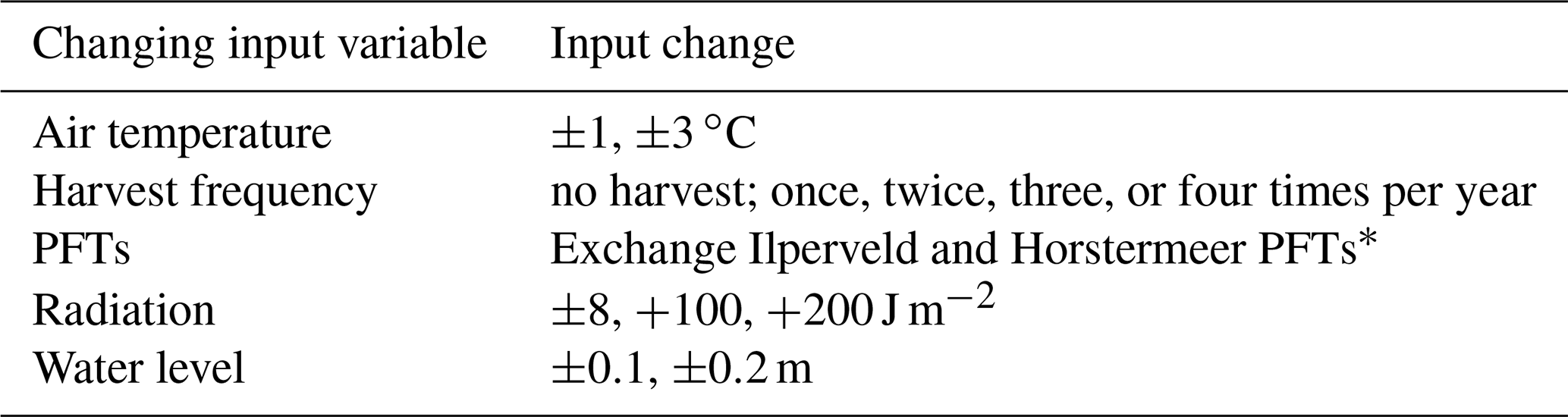
^* To compare the PFT dynamics, both simulations use the no-harvest regime. The exchange of PFTs means that the model simulation driven by the Ilperveld input data (Table 4) will use the PFTs observed at the Horstermeer site (Typha, tall grass, sedges, brown moss), while the model simulation driven by the Horstermeer input data will use the PFTs observed at the Ilperveld site (short grass, tall grass, Sphagnum, brown moss).

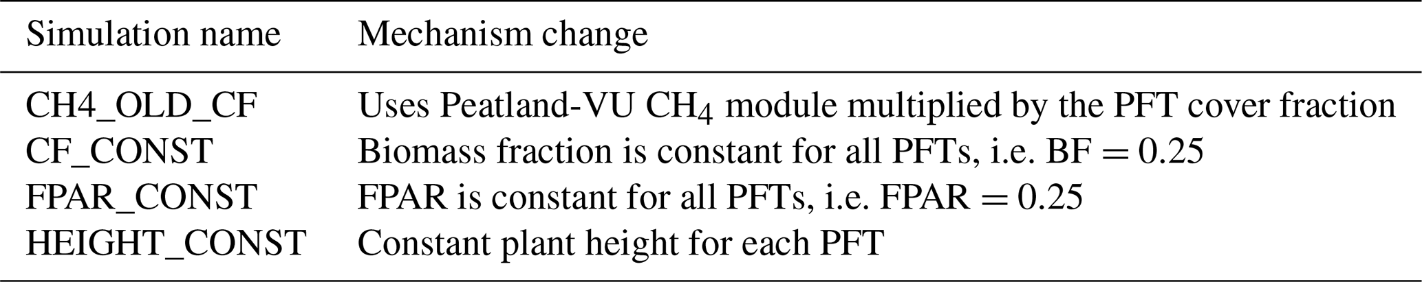
To understand how the new model mechanisms affect emissions, we performed additional simulations with altered model algorithms and compared these to the original model simulations calibrated for the Horstermeer and Ilperveld sites (Table 3). For example, the contribution of competition for shading to the overall simulation result is quantified by comparing an altered simulation where incoming photosynthetically active radiation (PAR) is independent of shading (e.g. fractional par or FPAR =0.25 for a simulation with four PFTs) to the original model simulations (FPAR_CONST). We calculated the relative difference of the simulation with shading minus the simulation without shading. Similarly, we compared simulations with and without plant-transported CH₄ (CH4_OLD_CF), with and without dynamic BF (CF_CONST), and with and without variable plant height (HEIGHT_CONST).

Table 3 A summary of the simulations with altered model algorithms.

In order to demonstrate that the PVN model reproduces CH₄ and CO₂ fluxes within the spread of observed fluxes when driven by realistic input data, we compared the calibrated model simulation results and measured CH₄ and CO₂ fluxes for the Horstermeer and the Ilperveld field sites (Sect. 2.2).

We compare the CH₄ and CO₂ fluxes of the calibrated model simulation results against the CH₄ and CO₂ fluxes simulated by the Peatland-VU model to understand the impact of introducing PFTs on the simulation of CH₄ and CO₂ fluxes. These model simulations are summarised in Table 4. Attempts to run the Peatland-VU model with new calibrated parameters did not yield results on the same order of magnitude as the observations. Therefore, it was necessary to use different model parameterisations for the PVN and Peatland-VU models.

2.6 Flux measurements

Carbon dioxide and CH₄ fluxes were measured using two to four automated flux chambers (AC) and the Ultra-Portable Los Gatos Gas Analyser Model 915-001. Chambers were cylindrical, 30 cm wide and 40 cm in height, made of transparent acrylate, equipped with a fan, and installed in the field using collars. Where necessary, vegetation was folded gently to fit inside the measurement chambers. Collars were removed from the field between sampling campaigns, which minimises disturbance which can lead to potential biases in the observations. This also potentially introduces uncertainty with regard to the precise measurement location. The CO₂ and CH₄ concentrations were measured for 150 s intervals whilst the chamber was closed. Each chamber was measured on rotation so that a new chamber was measured every 15 min. Measurements were recorded continuously during the day and night for a week at a time, during which time the AC system was moved to another site. We note that, due to the labour-intensive nature of accumulating chamber observations consistently through time, these observational datasets do not offer complete temporal continuity, creating an intermittency bias. From these data, the hourly average CO₂ (net ecosystem exchange) and CH₄ fluxes were calculated for each day. We compared calibrated site simulations against observed daily average CO₂ and CH₄ fluxes. To visualise the daily variability, standard deviations were derived from the hourly fluxes. The values for all GHG emissions are expressed as CO₂ equivalents [$\mathrm{kg}{\mathrm{CO}}_{\mathrm{2}\mathrm{eq}}{\mathrm{m}}^{-\mathrm{2}}{\mathrm{yr}}^{-\mathrm{1}}$] and are calculated as

$$\begin{array}{}\text{(32)}& {\mathrm{GHG}}_{{\mathrm{CO}}_{\mathrm{2}}e}={\mathrm{CH}}_{\mathrm{4}}\cdot \mathrm{GWP}+{\mathrm{CO}}_{\mathrm{2}},\end{array}$$

where GWP₂₀=80.8 as 1 kg CH₄ =80.8 kg CO₂ eq. over a 20-year time horizon, and GWP₁₀₀=27.2 as 1 kg CH₄ =27.2 kg CO₂ eq. over a 100-year time horizon (Masson-Delmotte et al., 2021).

2.7 Input data preparation

The PVN model is driven by daily air temperature (T), water level (WL), radiation, a general model parameter input file (Table S4), and a soil parameter input file (Table S5).

2.7.1 Climatological input data

Daily temperature and radiation data, measured at Schiphol, the nearest KNMI weather station, were used as climate input data for both sites (accessed via https://www.knmi.nl/nederland-nu/klimatologie/daggegevens, last access: 18 May 2022) (Fig. S3). The annual average rainfall at Schiphol was 850 mm yr⁻¹ over the period 1990–2020, with 30 % of the rainfall falling in summer and autumn and 24 % falling in winter, with the remainder falling in the spring. The average daily temperature between 1990 and 2019 was 9.4 ^∘C and warmed by approximately +0.1 ${}^{\circ }{\mathrm{Cyr}}^{-\mathrm{1}}$ over the same period. The average daily temperature for the warmest month, August, was 22.1 ^∘C, and the lowest daily monthly temperature for the coldest month, January, was 0.8 ^∘C.

2.7.2 Soil profile input data

The model generates a soil horizon representation using soil layers of 10 cm thickness. The generated soil horizon uses properties such as the dry bulk density (DBD), SOM ratio, sand content, and C:N ratio specified in the soil profile input data (Table S5). The number and depths of the site's soil horizons can be adjusted in the soil input file. The PVN model requires input parameters for each PFT, as discussed in Sect. 2.3. Soil profile data from the Horstermeer and Ilperveld field sites were collected in 2015 and 2016 and include DBD, C content, SOM content, sand and clay content, and pF curve (Tables S8 and S9 for the Horstermeer and Ilperveld site simulations, respectively).

2.7.3 Water level input data

Water level input data were sourced from the Dutch hydrological model, the Netherlands Hydrological Instrument (NHI) (De Lange et al., 2014), which has a reasonably high spatial resolution (250 m ×250 m). One aim of developing the PVN model is to eventually develop a model of all Dutch peatlands in conjunction with the NHI product. For this reason, the NHI product is used in this application of the model. The NHI water level output was converted to relative surface height using a 5 m ×5 m digital elevation map of the Netherlands, Actueel Hoogtebestand Nederland (Alhoz et al., 2020). It is possible to use in situ water levels as input data for the model, but these data were, unfortunately, unavailable for the duration of the simulation. The input data used for both sites are accessible from the Bitbucket repository: http://www.bitbucket.org/tlippmann/pvn_public (last access: 15 November 2023).

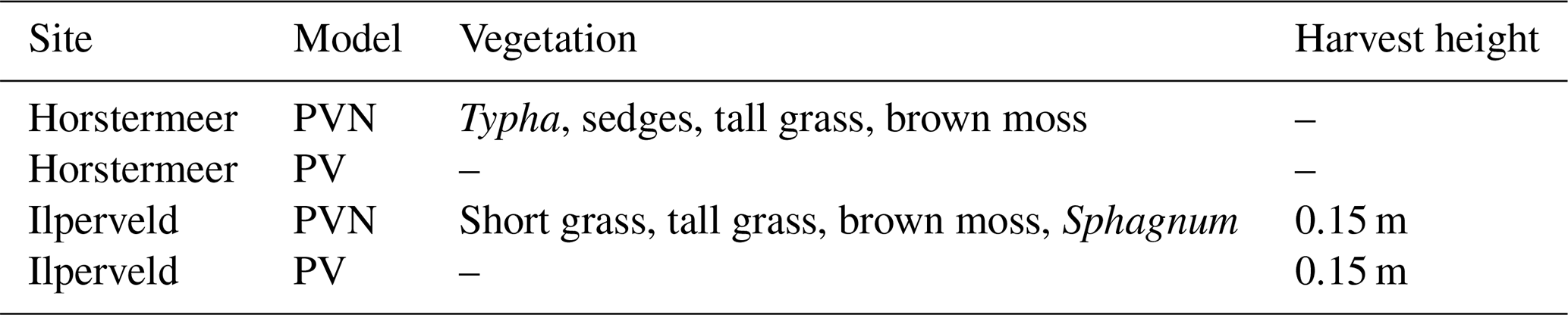
Table 4 A summary of the model simulations using both the new PVN model and the pre-existing Peatland-VU (PV) model. Model input parameters for the Horstermeer and Ilperveld site simulations are provided in Tables S6 and S7, respectively.

3 Results

When describing the annual CO₂, CH₄, and GHG values, we opt to use the term emissions, e.g. annual GHG emissions, whereas, when describing daily values, we opt to refer to these as fluxes, e.g. daily GHG fluxes.

3.1 Model sensitivity to input data

To understand the response of the modelled PFT processes to input data, we ran simulations with modified water levels (Figs. 3 and S6), temperature (Figs. 2 and S5), and radiation (Fig. S7) input and harvest schemes (Fig. 4). The modified input data are summarised in Table 2, and the results of these sensitivity tests are summarised in Table 5. These results are indicative of the model's mechanistic responses rather than being projections of how PFTs might respond under varied environmental conditions. To show how different inputs impact model processes, we present the soil (respiration) CO₂ emissions (Fig. 3), plant-transported CH₄ (Fig. 2), and aboveground biomass (Fig. 4). In the PVN model, the abundance of each PFT varies through time depending on the favourability of growing conditions. Therefore, an increase in CO₂ or CH₄ emissions may be due to increased abundance (i.e. enhanced biomass) or enhanced transport efficiency. To disentangle this difference, the CO₂ and CH₄ emissions for each PFT are plotted as a fraction of litter and root mass.

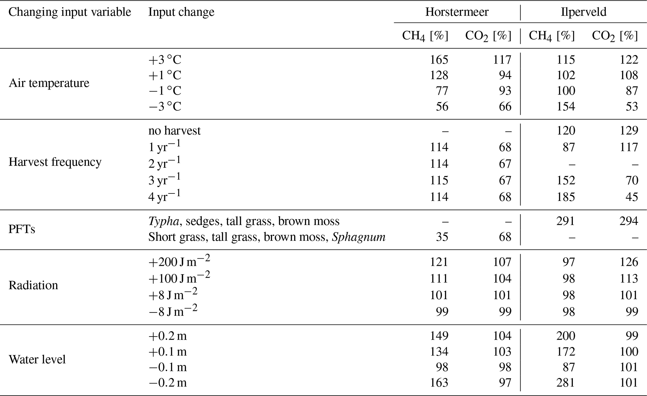
Table 5 The results of the sensitivity testing. The CH₄ and CO₂ columns indicate how much the respective emissions changed when the input changed relative to the results of the respective default Horstermeer and Ilperveld PVN simulations described in Table 4. A dash [–] indicates that the simulation is the default site simulation. An overview of the sensitivity tests can be found in Table 2.

Increased air temperatures had a positive effect on both plant-transported CH₄ emissions (Fig. 2) and litter and root mass at both sites (Fig. S5). Short and tall grasses showed similar responses to increased air temperatures by producing large CH₄ emissions per kilogram of litter and root mass. Brown mosses showed little variation between the temperature experiments for the Ilperveld site but showed a decrease in emissions with warming temperatures per kilogram of litter and root mass at the Horstermeer site. Sphagnum similarly showed a decrease in CH₄ emissions with warming temperatures per kilogram of litter and root mass at the Ilperveld site. This decrease is because moss PFTs have strict ideal-temperature growth limits (T_max and T_min in Table 1) and were limited by warming temperatures. Whilst belowground, CH₄ concentrations increased with warming temperatures, and the biomass, litter, and root mass of moss PFTs did not increase with warming temperatures.

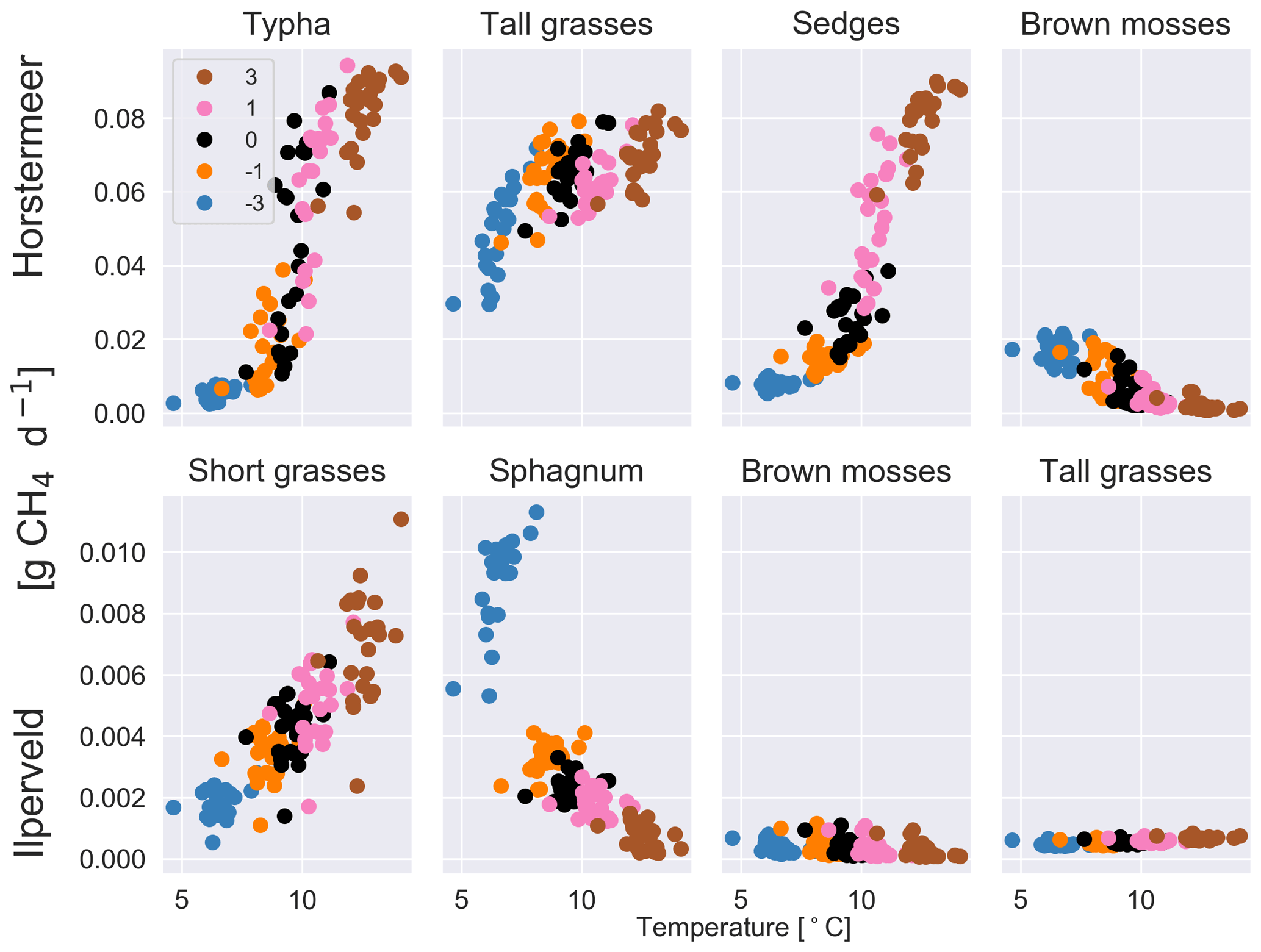
Figure 2 The results of the sensitivity tests show the relationship between different temperature inputs and the mean daily plant-transported CH₄ for each year for each of the PFTs at the Horstermeer site (top row) and Ilperveld site (bottom row). Temperature input was increased and decreased by 1 and 3 ^∘C, respectively. The legend shows the input change [^∘C] where ± signs in front of the legend labels show the direction of change. Note the different y axes between the top and bottom panels.

Belowground CO₂ emissions were impacted by changing water levels (Fig. S6). Previous studies have found that belowground CO₂ production tends to increase with low water levels due to enhanced potential for aerobic CO₂ production (Knox et al., 2015). The results of the Ilperveld site sensitivity simulations showed that belowground CO₂ production increased with low water levels, likely due to enhanced potential for aerobic CO₂ production. However, the results of the Horstermeer site sensitivity simulations showed the converse: that the net CO₂ (Table 5) and belowground CO₂ production increased with high water levels. We simulate that, with high water levels, the reduced aerobic CO₂ production can be exceeded by the enhanced oxidation of CH₄ into CO₂. The large amounts of CH₄ oxidised into CO₂ in the Horstermeer site simulation are due to the very degraded peat present at the site (represented by low soil OM content in the soil input file) and the strong upwelling of rich groundwater at the Horstermeer site (represented by the calibratable model parameter, MolAct (see Sect. 2.4), which influences the sensitivity of aerobic CO₂ production). The large observed CH₄ emissions at the Horstermeer site are partially due to high CH₄ concentrations in the upwelling water. Furthermore, the large root systems of plants such as Typha, sedges, and tall grasses have greater potential to access and transport stores of belowground gases (represented by the PFT root depth and mass). The conflicting response of the tall grass PFT in the Ilperveld and Horstermeer simulations shows that PFTs may respond differently to changing water levels at different sites.

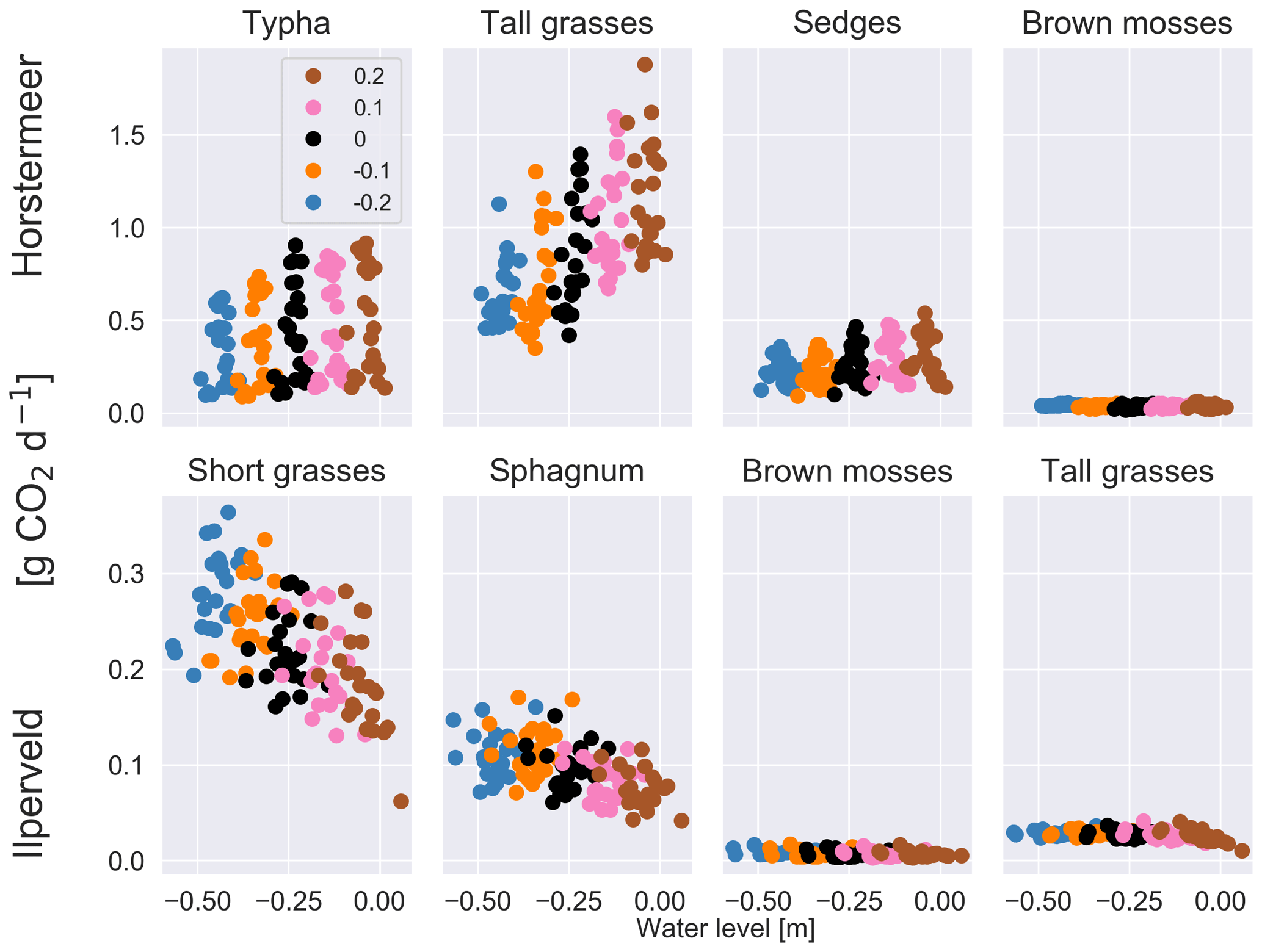
Figure 3 The results of the sensitivity tests show the relationship between different water level inputs and the mean daily soil CO₂ flux for each year for each of the PFTs at the Horstermeer site (top row) and the Ilperveld site (bottom row). Water level input was decreased by 0.1 and 0.2 m and was increased by 0.1 and 0.2 m, respectively. The legend shows the input change, where ± signs in front of the legend labels indicate the direction of the change. Note the different y axes between the top and bottom panels.

Increasing the frequency of harvests led to a strong negative effect on vascular plant biomass and a small positive effect on moss plant biomass (Fig. 4). The biomass of non-moss PFTs is strongly impacted by the occurrence of harvests, as indicated by the pause in biomass accumulation after harvest. However, by reducing tall vegetation, moss species have greater access to sunlight and, therefore, gain an advantage. For this reason, we saw the biomass of moss PFTs increase with more frequent harvests. In the Horstermeer site simulation, the greatest effect on biomass was between no harvests and the once-per-year harvests. In the Ilperveld site simulation, the effects of harvests on biomass increased somewhat linearly according to the frequency of harvest events. We suspect that this is due to the inclusion of different PFTs in the two site simulations. In the Horstermeer site simulation, three PFTs have the capacity to grow above the harvest height (the Typha, tall grass, and sedge PFTs), whereas in the Ilperveld site simulation, only tall and short grasses have the potential to grow beyond the harvest height, thereby limiting the potential effect harvests can have on the PFTs present. Furthermore, the growth of the short grass PFT is height limited to 0.3 m. Overall, total biomass was reduced with more frequent harvest regimes.

It is important to note that, whilst CO₂ emissions were reduced by increasing the frequency of harvests, these emissions do not account for the off-site decomposition of harvested biomass. Methane emissions were slightly enhanced if harvests occurred in comparison to no harvest events for Horstermeer site simulations, whilst the frequency of harvests did not impact emissions (Table 5). Similarly, enhanced CH₄ emissions occurred with increased harvest frequency for the Ilperveld site simulations. Spikes in CH₄ fluxes transported by vascular PFTs occurred after harvest events in both the Horstermeer and Ilperveld simulation results (not shown), contributing to enhanced CH₄ emissions for both the Ilperveld and Horstermeer site simulations. The impact of fewer or no harvest events led to variable impacts on CH₄ emissions for the Ilperveld site simulations, where a single harvest led to slightly reduced emissions, and no harvests led to slightly enhanced emissions. In the Ilperveld site simulation without harvest events, vegetation became dominated by vascular PFTs that are efficient transporters of CH₄, leading to enhanced CH₄ emissions.

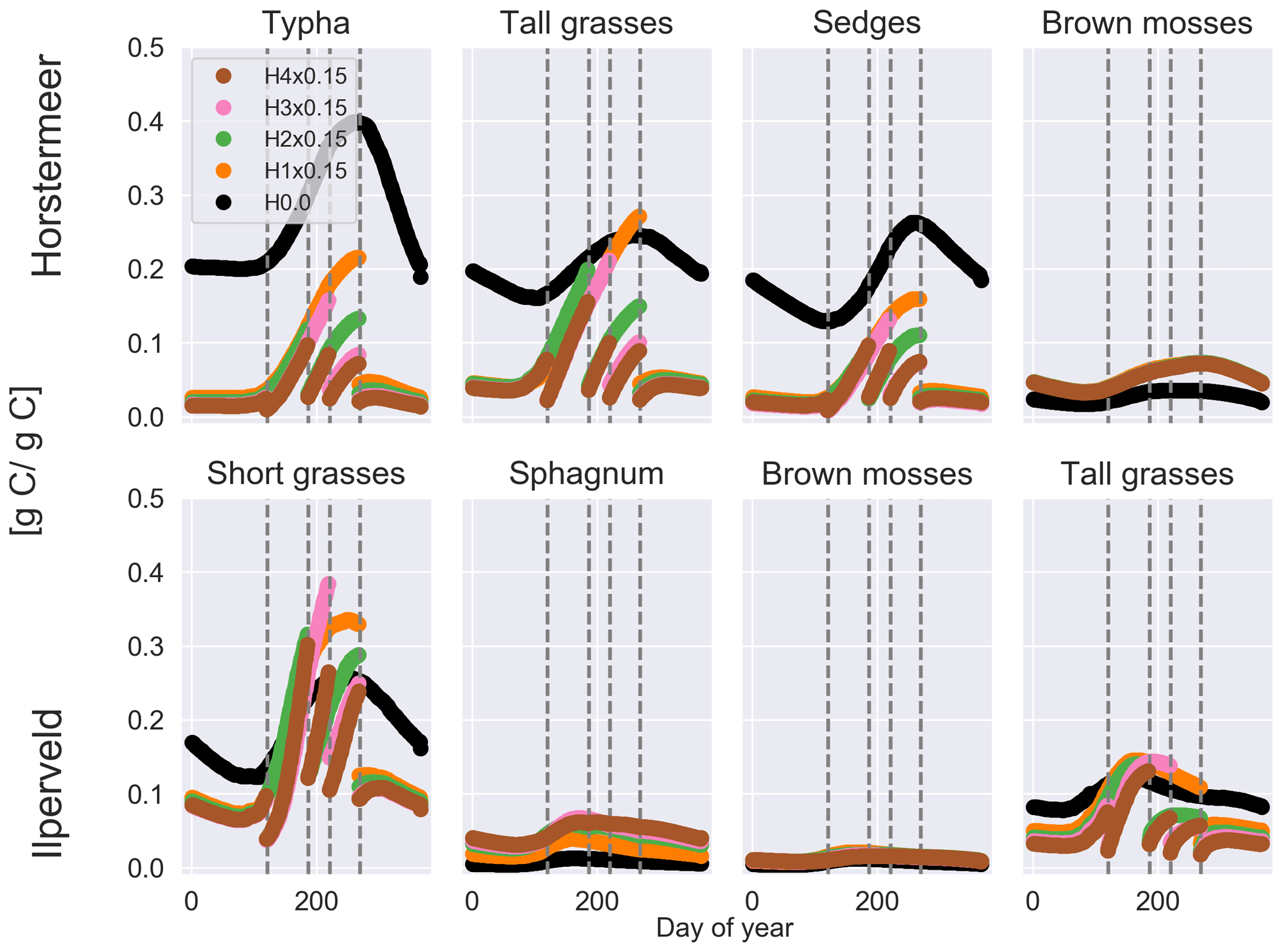
Figure 4 The results of the sensitivity tests show the relationship between different harvest schemes and biomass for each day of year (shown as a fraction of litter and root mass) at the Horstermeer site (top row) and Ilperveld site (bottom row). Vegetation is cut to 0.15 m (×0.15) at the moment of harvest. The legend shows the harvest input scheme, and the vertical dotted lines indicate the four possible harvest days (days 120, 186, 220, and 268). Harvest was set to either not occur (H0.0) or to occur once per year (H1x0.15) on day 268, twice per year (H2x0.15) on days 186 and 268, three times per year (H3x0.15) on days 120, 220 and 268, or four times per year (H4x0.15) on all harvest days.

3.2 Assessment of model mechanisms

To understand the role of isolated model mechanisms, we modified the model code to disable the functions responsible for reproducing the vegetation dynamics within the model (Fig. 5). Unlike the other simulations assessed throughout this paper, the simulation results shown in Fig. 5 begin in the year 1990, i.e. without the use of a spin-up period. Removing the spin-up period showed that the modified model simulation results produce similar emissions in the first year of the simulation (1990) and allows an assessment of the trajectory of deviation.

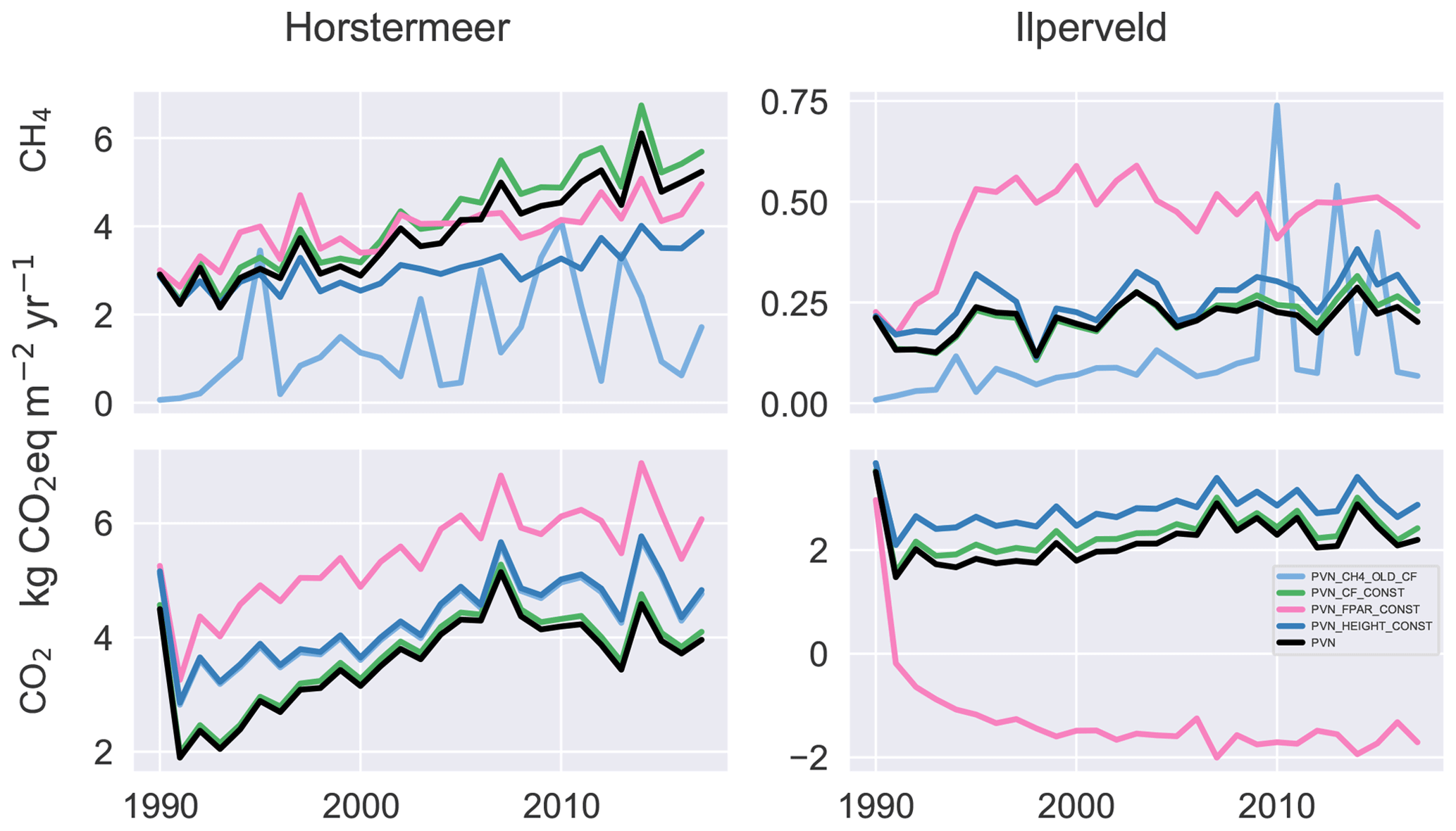
Figure 5 The CH₄ and CO₂ emissions for various isolated model mechanisms compared against the PVN model result. We investigated maintaining constant fractional PAR (PVN_FPAR_CONST), maintaining constant plant height (PVN_HEIGHT_CONST), maintaining constant cover fraction (PVN_CF_CONST), and including the original Peatland-VU CH₄ module multiplied by the PFT cover fraction (PVN_CH4_OLD_CF) at each time step.

Disabling the shading scheme (simulation PVN_HEIGHT_CONST) or biomass fraction scheme (simulation PVN_CF_CONST) led to only slightly enhanced CO₂ emissions, whereas disabling the FPAR scheme (simulation PVN_FPAR_CONST) led to large CO₂ emission differences. Surprisingly, the difference for the PVN_FPAR_CONST simulation is opposite in sign for the two site simulations and is larger for the Ilperveld simulation. This means that maintaining constant FPAR led to a small enhancement in CO₂ emissions in the Horstermeer simulation but a large reduction in CO₂ emissions for the Ilperveld simulation. These results show that FPAR plays a large role in simulated CO₂ emissions. The results of the Ilperveld PVN_FPAR_CONST simulation also showed that the FPAR function has the potential to introduce large variability into the emission results. This is interesting to note because the PVN model showed limited skill in reproducing the CO₂ emissions at the Ilperveld site. These results indicate that the function calculating FPAR plays a driving role in CO₂ emissions but particularly at the Ilperveld site. Further model developments may investigate ways to improve the representation of FPAR in the model. The PVN_FPAR_CONST simulations also led to enhanced CH₄ emissions for the Ilperveld simulation. It is likely that CH₄ production was enhanced due to increased stores of CO₂.

The use of the Peatland-VU CH₄ scheme (PVN_CH4_OLD_CF) led to large differences in CH₄ emissions for both the Horstermeer and Ilperveld simulations in comparison to the PVN model results. The CH₄ emissions of the model simulations that use the Peatland-VU CH₄ scheme (simulation PVN_CH4_OLD_CF) were small when compared to the CH₄ emissions of the PVN model for both model simulations. This indicates that the PFT modifications to the CH₄ scheme have led to substantial impacts on modelled CH₄ emissions.

3.3 Assessment of calibrated model simulations

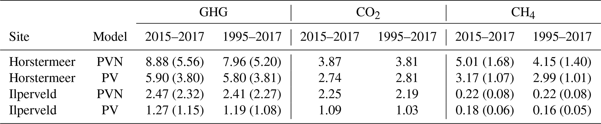
Here, we describe the simulation results of the model calibrated at two field sites, Horstermeer and Ilperveld. We describe the net annual CH₄ and CO₂ emissions and GHG budgets (Fig. 6), as well as the simulated PFT dynamics as indicated by changes to LAI, aboveground biomass, litter mass, and PFT height and/or depth (Figs. 7 and S8). All net GHG values are expressed as CO₂ equivalents (CO₂ eq.). The model simulation results indicate that the simulated annual mean net GHG emissions from the Ilperveld simulation were approximately half the emissions of the Horstermeer simulation. However, these model emission estimates do not consider off-site decomposition of harvested biomass. The model estimated that the 2015–2017 annual average net GHG emissions were 2.5 and 8.9 $\mathrm{kg}{\mathrm{CO}}_{\mathrm{2}}\mathrm{eq}.{\mathrm{m}}^{-\mathrm{2}}{\mathrm{yr}}^{-\mathrm{1}}$ for the Ilperveld and Horstermeer simulations, respectively (Table 6), calculated using the 20-year GWP. Using the 100-year GWP, the 2015–2017 annual average net GHG emissions were 2.3 and 5.6 $\mathrm{kg}{\mathrm{CO}}_{\mathrm{2}}\mathrm{eq}.{\mathrm{m}}^{-\mathrm{2}}{\mathrm{yr}}^{-\mathrm{1}}$ for the Ilperveld and Horstermeer simulations, respectively. The model estimated that the 1995–2017 annual average net GHG emissions were 2.4 and 8.0 $\mathrm{kg}{\mathrm{CO}}_{\mathrm{2}}\mathrm{eq}.{\mathrm{m}}^{-\mathrm{2}}{\mathrm{yr}}^{-\mathrm{1}}$ for the Ilperveld and Horstermeer model simulation results, respectively (Fig. 6), calculated using the 20-year GWP. Using the 100-year GWP, the 1995–2017 annual average net GHG emissions were estimated to be 2.3 and 5.2 $\mathrm{kg}{\mathrm{CO}}_{\mathrm{2}}\mathrm{eq}.{\mathrm{m}}^{-\mathrm{2}}{\mathrm{yr}}^{-\mathrm{1}}$ for the Ilperveld and Horstermeer model simulation results, respectively.

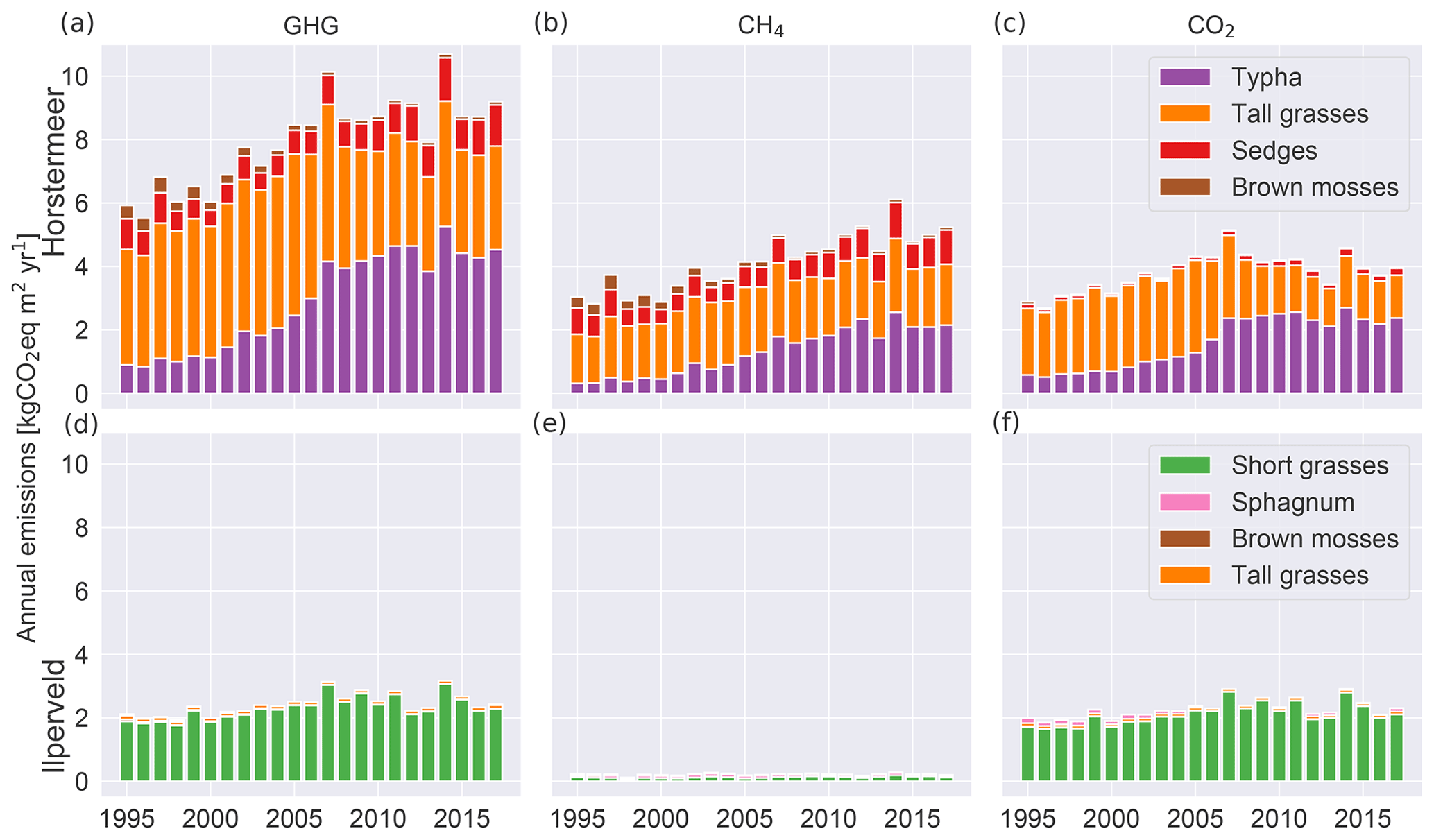
Figure 6 Relative contributions of each PFT to simulated annual average net GHG (a, d), CH₄ (b, e), and CO₂ (c, f) emissions. The results of the Horstermeer site simulation are represented in (a)–(c), and the results of the Ilperveld site simulation are represented in (d)–(f).

Assessment of the Horstermeer simulation showed that, on average, CH₄ contributed approximately half (52 %) of the net annual GHG emissions of the Horstermeer simulation, where CH₄ contributed 4.2 $\mathrm{kg}{\mathrm{CO}}_{\mathrm{2}}\mathrm{eq}.{\mathrm{m}}^{-\mathrm{2}}{\mathrm{yr}}^{-\mathrm{1}}$ and CO₂ emissions contributed 3.8 $\mathrm{kg}{\mathrm{CO}}_{\mathrm{2}}\mathrm{eq}.{\mathrm{m}}^{-\mathrm{2}}{\mathrm{yr}}^{-\mathrm{1}}$, on average. Assessment of the Ilperveld simulation showed that CO₂ was the primary contributor to net GHG emissions, where CO₂ contributed the majority (92 %) of the annual GHG emissions (2.2 $\mathrm{kg}{\mathrm{CO}}_{\mathrm{2}}\mathrm{eq}.{\mathrm{m}}^{-\mathrm{2}}{\mathrm{yr}}^{-\mathrm{1}}$ of the total 2.4 $\mathrm{kg}{\mathrm{CO}}_{\mathrm{2}}\mathrm{eq}.{\mathrm{m}}^{-\mathrm{2}}{\mathrm{yr}}^{-\mathrm{1}}$ net GHG emissions). These model emission estimates neglect the off-site decomposition of harvested biomass. Therefore, CO₂ and CH₄ emissions contribute equally to the net GHG emissions in the Horstermeer simulation, whereas CO₂ emissions dominate the GHG emissions in the Ilperveld simulation results.

To assess whether there was an increasing or decreasing trend in emissions over the duration of the simulation (1995–2017), we calculated the linear regression of the CO₂, CH₄, and net GHG time series of the simulation results at both sites. The trends of the Horstermeer simulation emission results were 0.13, 0.06, and 0.19 $\mathrm{kg}{\mathrm{CO}}_{\mathrm{2}}\mathrm{eq}.{\mathrm{m}}^{-\mathrm{2}}{\mathrm{yr}}^{-\mathrm{1}}$ for CH₄, CO₂, and the net GHG emissions. Daily temperature observations show that local temperatures increased by +0.1 ^∘C yr⁻¹ between 2010 and 2017 or +0.06 ^∘C yr⁻¹ over the entire simulation period (1995–2017). The trend results for the Ilperveld simulation emissions were zero for CH₄ emissions and 0.04 $\mathrm{kg}{\mathrm{CO}}_{\mathrm{2}}\mathrm{eq}.{\mathrm{m}}^{-\mathrm{2}}{\mathrm{yr}}^{-\mathrm{1}}$ for CO₂ and net GHG emissions. Warming temperatures are a possible driver of the enhanced GHG emissions at the Horstermeer site. The increase in GHG emissions in the Horstermeer site simulation and the little or no increase in the Ilperveld site simulation are aligned with the results of the +1 ^∘C temperature sensitivity tests. The results of the Horstermeer site sensitivity tests showed that the Typha and sedge PFTs were sensitive to warming temperatures; therefore, the increases in the biomass and GHG emissions of the Typha and sedge PFTs at the Horstermeer site are likely due to enhanced temperatures.

3.3.1 PFT dynamics

Here, we describe the living biomass, LAI, litter layer, biomass fraction, and height changes of the PFTs of the calibrated Horstermeer and Ilperveld model simulations (Figs. 7 and S8). Assessment of the aboveground biomass (top row of Fig. 7) shows that the tall grass (blue line), Typha, and sedge PFTs (red line) were abundant during the Horstermeer simulation. whereas the Ilperveld simulation was dominated by the short grass (green line), Sphagnum (pink line), and tall grass PFT (blue line). All plants showed seasonal variability. The ratio of the litter layer to biomass is between approximately 1:4 and 1:3 for most PFTs [kg C]. The Typha PFT is an exception, and the ratio is approximately 1:1. Overall, the sedge PFT showed comparable seasonal variability to the tall grass PFT whilst maintaining less biomass, smaller LAI, and shorter height throughout the Horstermeer simulation. The similar behaviour of the Typha, sedge, and tall grass PFTs was expected because the PFT input parameters represent similar plant phenologies. Assessment of the size of the litter layer (first row of Fig. S8) showed that, in the Ilperveld simulation, the PFTs reached peak litter during autumn (September), whilst in the Horstermeer simulation, which is not mown, the litter continued to accumulate until January, where rates of decomposition exceeded accumulation. The LAI (second row of Fig. S8) displayed strong seasonal variability. Each year, the LAI of the short grasses reaches its maximum LAI value of 1.2. The tall grass PFT, whilst very competitive in the Horstermeer simulation, is less competitive in the Ilperveld simulation, partially due to the occurrence of harvests and partially because it is outcompeted by the fast-growing short grass PFT. Assessment of the Ilperveld simulation reveals that the short grass PFTs were constrained by the maximum-height parameter, MaxCanopyHeight. The tall grass PFT was not limited by MaxCanopyHeight in the Ilperveld simulation but was instead limited by the biannual mowing regime. PFT height showed strong seasonal variability for both simulations (third row of Fig. S8). The tall grass PFT constituted the tallest plants in the Horstermeer simulation until 2009, and its height was frequently limited by the PFT MaxCanopyHeight parameter. However, as the Typha PFT grew in biomass, the tall grass PFT appeared to have less access to sunlight as height and biomass values were reduced. The Typha and sedge PFTs were not limited by their maximum-height parameters. These changes in biomass fraction are also evident in the emissions.

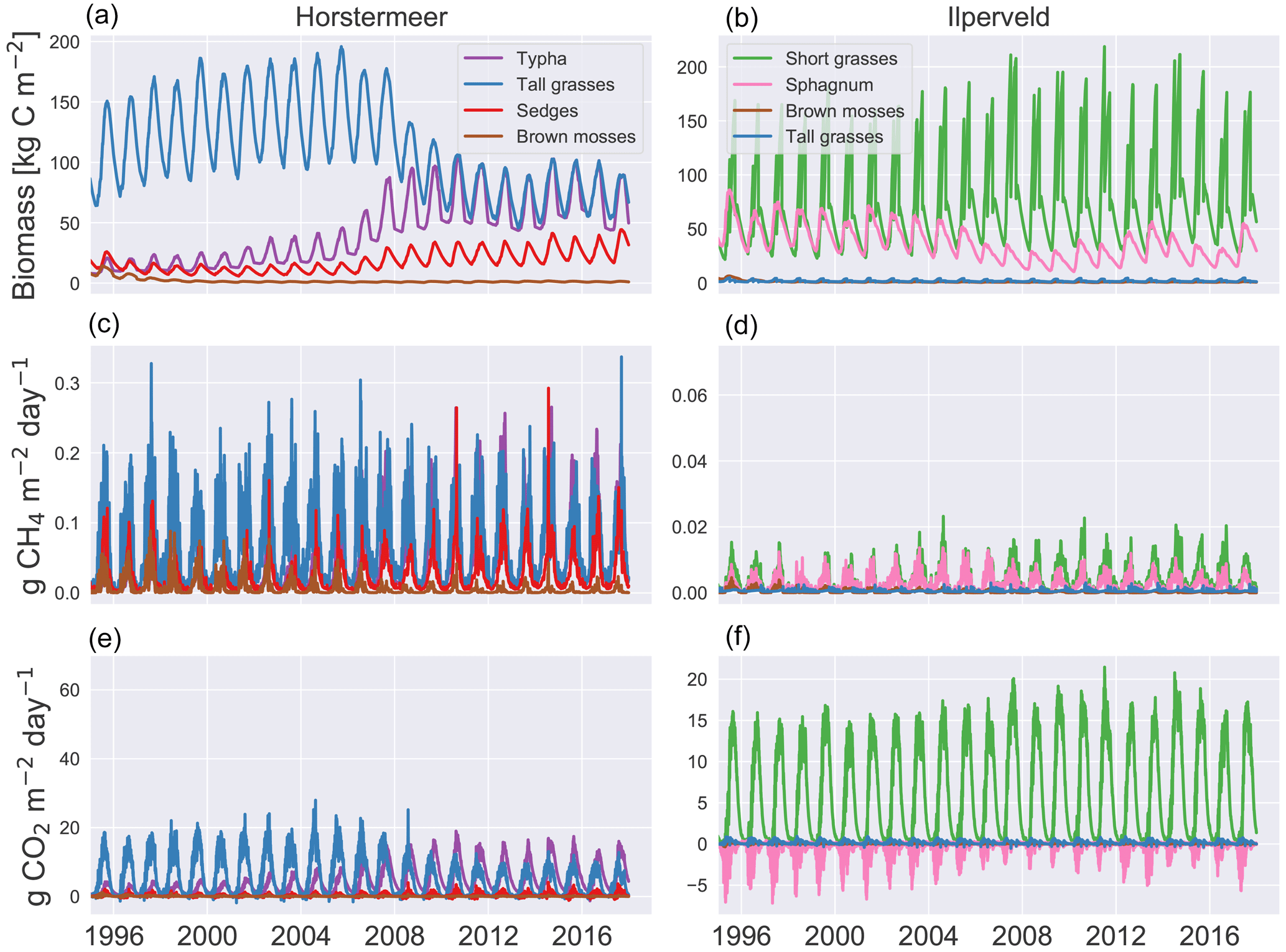
Figure 7 Vegetation dynamics. The results of the Horstermeer site simulation are represented in (a), (c), and (e), and the results of the Ilperveld site simulation are represented in (b), (d), and (f). Note the differing y axes.

The relative contributions of each PFT to the net annual CH₄, CO₂, and GHG emissions are shown in Fig. 6, where the CH₄ emissions refer to only the plant-transported CH₄. The net CO₂ emissions for each PFT are the sum of the photosynthesis minus respiration, the CO₂ produced by belowground aerobic decomposition of SOM, and a portion of CH₄ oxidised to CO₂. The tall grass (red boxes), sedge (orange boxes), and Typha (purple boxes) PFTs are large transporters of CH₄ emissions in the Horstermeer simulation results. However, only the tall grasses and Typha compose the net CO₂ emissions in the Horstermeer simulation. Thereby, the tall grass PFT was the largest contributor to the net annual GHG emissions, followed by the Typha and sedge PFTs. The Ilperveld simulation results showed that the short grass PFT was the largest contributor to the net annual CH₄, CO₂, and GHG emissions.

3.4 Comparison of modelled and observed plant dynamics

We compare simulated PFT biomass fractions against observed aerial plant cover fractions (Fig. 8). For assessment against observational data, we compare model simulation results against observed fluxes by comparing time series, boxplots, and 1:1 scatterplots for CH₄ (Fig. 9) and CO₂ (Fig. 10). Gaps in observational data exist due to measurement collection limitations; therefore, the model comparison against observational data can only be shown for the days where observational data exist. Unfortunately, this means that the model was not assessed equally across all seasons or on the same days of the year at the two sites. A simple linear regression is used to compare the model simulation results and observational data using all days with available measurements. For these reasons, the 1:1 plots and R² linear regression results may only give a flavour of model performance. To understand the degree of uncertainty in the observational measurements, daily standard deviations were derived using the hourly fluxes (plotted as black error bars in Figs. 9 and 10). In each case, the model simulation results generally lay within the spread of observational uncertainty. The observations indicated that both sites are annual sources of CH₄ and CO₂ and, therefore, net annual sources of carbon to the atmosphere. The Horstermeer site produced large annual mean CH₄ and CO₂ emissions in comparison to the Ilperveld site (Fig. 9 and Fig. 10).

3.4.1 Evaluation of plant composition dynamics

Plant cover fraction observations were made at the location of the chamber measurements and were not representative of the site's complete plant community composition. Although aerial cover fraction and biomass fraction (the ratio of PFT biomass to total biomass) are not the same, changes in plant composition are depicted in both representations.

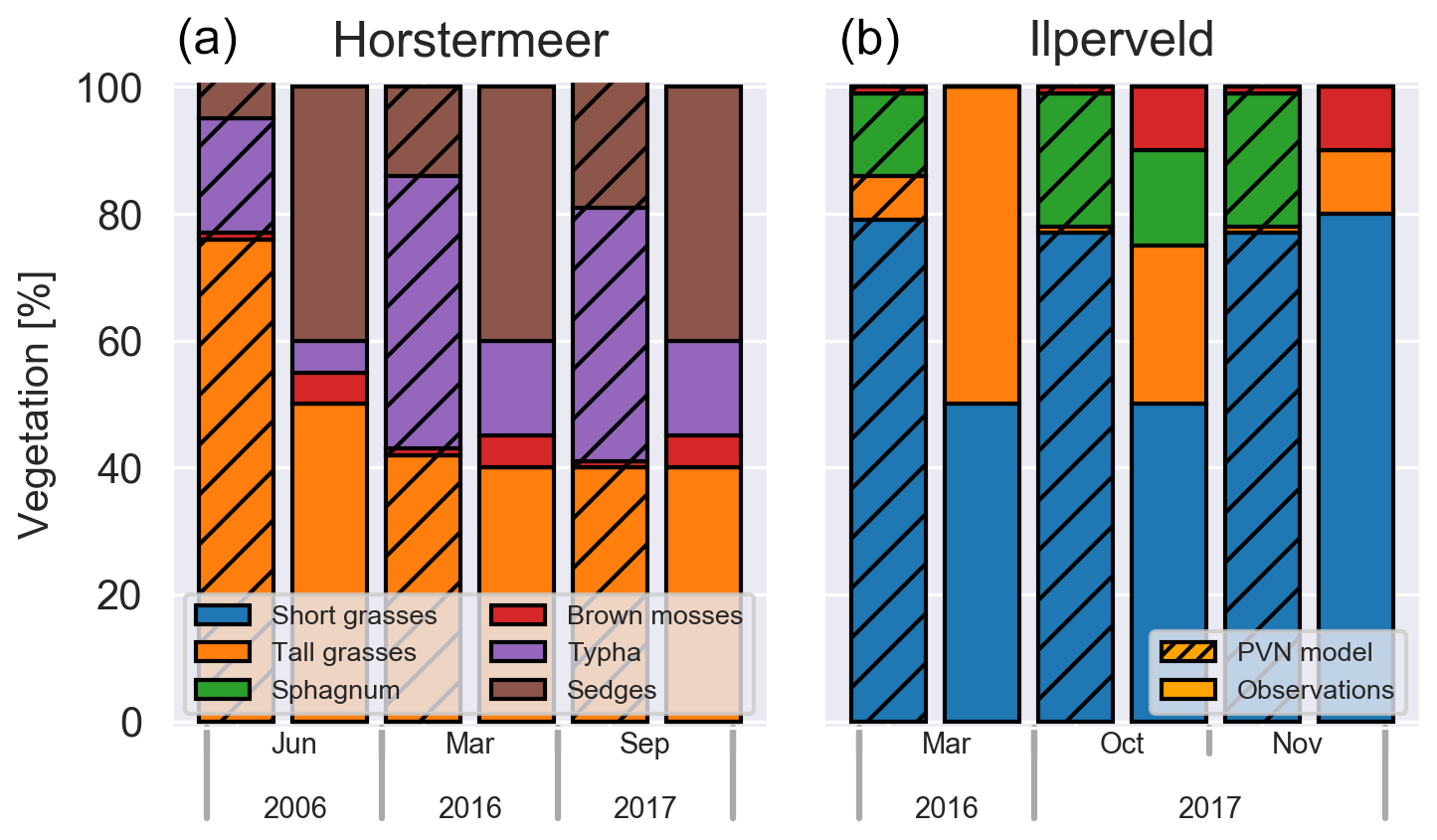
Figure 8 Simulated PFT biomass fractions and observed areal cover fractions at Horstermeer (a) and Ilperveld (b).

In 2006, the chamber measurement location at the Horstermeer field site was composed of tall grasses (50 %), sedges (40 %), Typha (5 %), and brown mosses (5 %) (left panel in Fig. 8). The Horstermeer simulation results show good agreement with the observations but overestimated the amount of tall grasses (66 %) and underestimated the amount of sedges (40 %). In 2016, a decade later, the amount of tall grasses remained consistent, whilst the amount of Typha had increased by 10 %; 1 year later, in 2017, the vegetation had not undergone changes proportionally. Parallel to the observations, the Horstermeer simulation results estimated that the tall grass PFTs decreased to 60 % from 2005 onwards, whilst the biomass fractions of the Typha and sedge PFTs increased. Overall, the Horstermeer simulation overestimated the biomass fraction of the tall grass PFT and underestimated the proportion of the sedge and Typha PFTs. Model estimates of year-to-year PFT biomass changes were of the same sign and similar magnitude as in situ observations.

In March 2016, the chamber measurement location at the Ilperveld field site hosted short grasses (50 %) and tall grasses (50 %). The model overestimated the amount of short grasses (80 %), underestimated the amount of tall grasses (5 %), and overestimated the amount of Sphagnum (10 %). The Omhoog met het Veen (Raising the Peat) project delivered on-site management attempts to initiate Sphagnum growth by hand dispersing living fragments of Sphagnum spp. from a nearby donor site between 2013 and 2015 (Geurts and Fritz, 2018). For this reason, we expected that the model may not match the development of Sphagnum at the Ilperveld site. In October 2017, the vegetation shifted to be composed of short grasses (50 %) and tall grasses (25 %), Sphagnum (15 %), and brown mosses (10 %); 1 month later, in November 2017, the Sphagnum was no longer visible (0 %), brown mosses remained (10 %), and the site was dominated by short grasses (80 %). The model estimated that the short grass and Sphagnum PFTs remained consistent into 2016 and 2017, whilst the tall grass PFT was reduced, and brown mosses increased slightly. Whilst the model simulations ended in 2017, we saw that, in October 2018, the vegetation remained constant at both sites.

3.4.2 Evaluation of simulated CH₄ fluxes

The time series presented in Fig. 9 shows the behaviour of the Horstermeer simulation CH₄ flux results (purple line), the observed mean daily fluxes (black dots), and the spread of the hourly observed fluxes (black error bars). Whilst the Horstermeer simulation reproduced the seasonal variability of the observed CH₄ fluxes, the boxplots showed that the simulation results (purple box) tended to overestimate the CH₄ fluxes. Overall, the Horstermeer simulation showed a robust pattern of variability when compared with the observations (R²=0.7) whilst overestimating the magnitude of observed fluxes. Assessment of the Ilperveld model simulation showed that the model was able to reproduce the observed CH₄ fluxes and followed the pattern of variability when compared with the observations (R²=0.8). The summer of 2015 is an exception where the simulated results showed an increase in CH₄ fluxes larger than the observed CH₄ fluxes. Assessment of the boxplots showed that the simulated CH₄ fluxes (green box) are of a similar mean and spread to the observed fluxes (purple box).

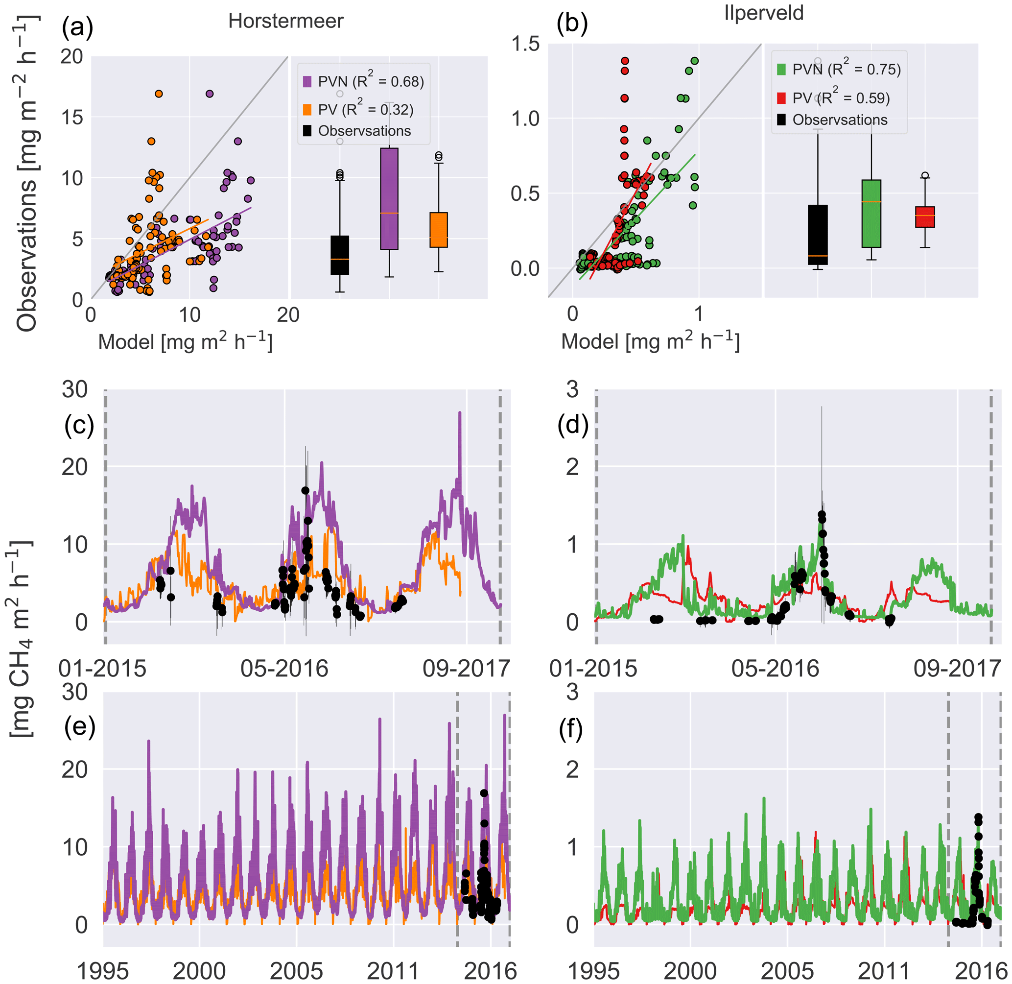
Figure 9 Simulated and observed methane fluxes at the Horstermeer (a, c, e) and Ilperveld (b, d, f) sites. The R² values are provided for comparison between the new PVN, the Peatland-VU model, and the observations. In (a) and (b), the 1:1 line is plotted in grey. The black dots are in situ flux chamber observational measurements in (c), (d), (e), and (f). Note the differing x and y axes.

3.4.3 Evaluation of simulated CO₂ fluxes

The boxplots showed that the PVN Horstermeer simulation reproduced the median and range of observed daily CO₂ fluxes at the Horstermeer site. The results of the Horstermeer site simulation (purple line) reproduced the 2015, 2016, and 2017 spring CO₂ fluxes. The results of the Horstermeer site simulation captured the 2015 and 2016 autumn fluxes. However, the model generally overestimated the magnitude of simulated fluxes (purple box) but generally reproduced the variability (R²=0.8).

The boxplots in Fig. 10 showed that the Ilperveld simulation results (green box) generally overestimated CO₂ fluxes. The boxplots showed that the mean hourly CO₂ flux simulated by the model was a small positive flux at 250 $\mathrm{mg}{\mathrm{CO}}_{\mathrm{2}}{\mathrm{m}}^{-\mathrm{2}}{\mathrm{h}}^{-\mathrm{1}}$, whereas the observed mean hourly flux was 0 $\mathrm{mg}{\mathrm{CO}}_{\mathrm{2}}{\mathrm{m}}^{-\mathrm{2}}{\mathrm{h}}^{-\mathrm{1}}$. The Ilperveld simulation (green line) captured the early-spring fluxes in 2016 and 2017. However, during 2015 and 2016, the model tended to overestimate the observed CO₂ fluxes. Comparison of the simulated daily hourly average (green line) and the spread of hourly fluxes (black error bars) showed that the simulated CO₂ fluxes (green line) fell within the spread of daily hourly fluxes. The model showed some agreement with the observed pattern of variability (R²=0.6).

The comparison between the Horstermeer simulation results and observations showed that the model captured the mean daily CO₂ fluxes but overestimated CH₄ fluxes. The comparison between the Ilperveld simulation results and the observations showed that the model overestimated the mean CO₂ fluxes but reproduced the mean and variability of CH₄ fluxes.

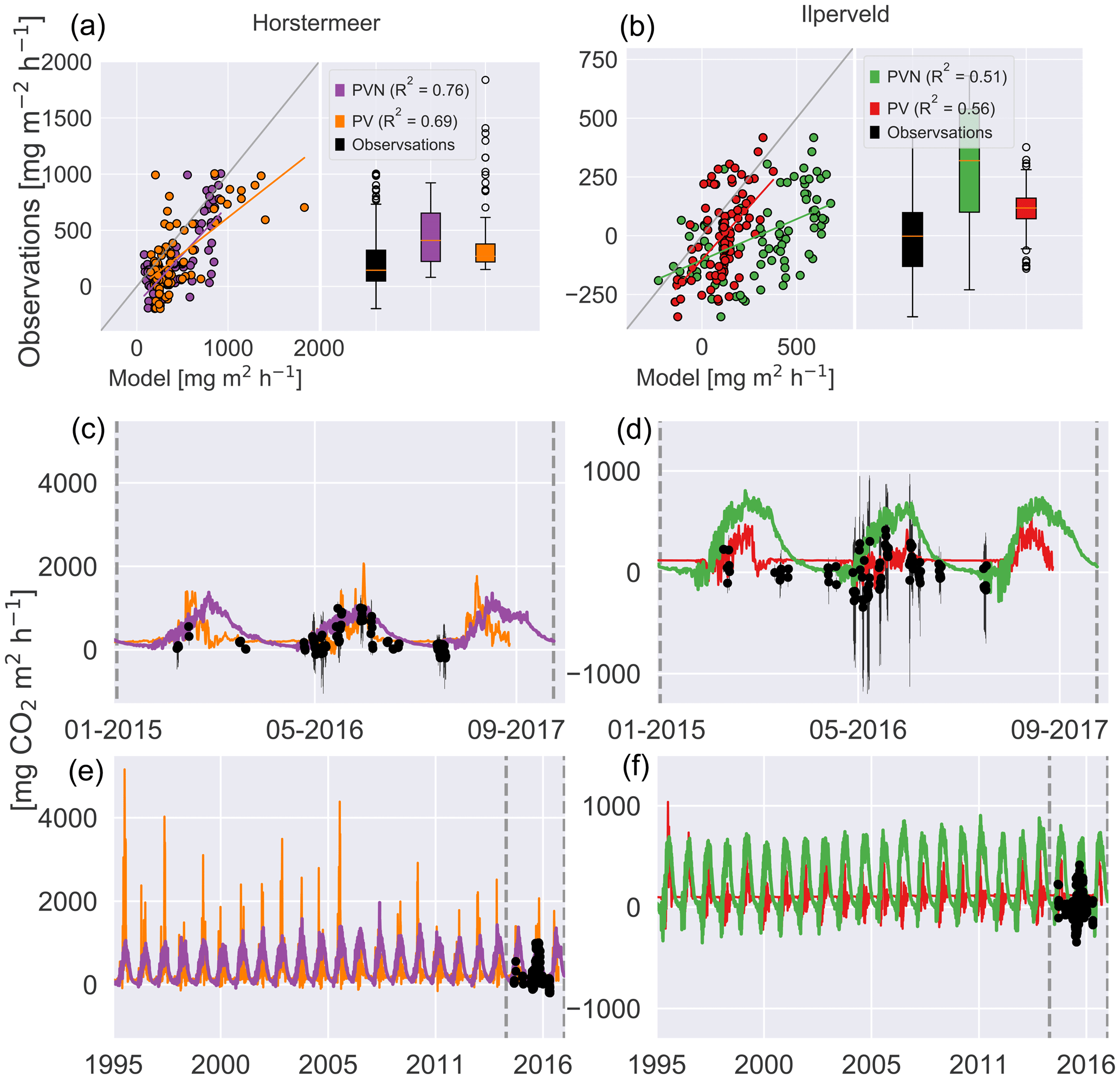
Figure 10 Simulated and observed carbon dioxide fluxes (NEE) at the Horstermeer (a, c, e) and Ilperveld (b, d, f) sites. The R² values are provided for comparison between the new PVN, the Peatland-VU model, and the observations. In (a) and (b), the 1:1 line is plotted in grey. The black dots are in situ flux chamber observational measurements in (c), (d), (e), and (f). Note the differing x and y axes.

3.5 Comparison to the PEATLAND-VU model

To understand the impact of including vegetation dynamics, we compare the results of the new PVN model against the results of the pre-existing Peatland-VU model (Fig. 9 and CO₂ in Fig. 10). The simulation results are summarised in Table 6. Overall, the PVN model estimated the net annual CH₄, CO₂, and GHG emissions to be larger than the emissions estimates made by the Peatland-VU model. The Peatland-VU model estimated the annual mean 2015–2017 GHG emissions to be 1.3 and 5.9 $\mathrm{kg}{\mathrm{CO}}_{\mathrm{2}}\mathrm{eq}.{\mathrm{m}}^{-\mathrm{2}}{\mathrm{yr}}^{-\mathrm{1}}$ for the Ilperveld and Horstermeer simulations, respectively, calculated using a 20-year GWP. When calculated using a 100-year GWP, the Peatland-VU model GHG emission estimates for the Horstermeer simulation were 3.8 $\mathrm{kg}{\mathrm{CO}}_{\mathrm{2}}\mathrm{eq}.{\mathrm{m}}^{-\mathrm{2}}{\mathrm{yr}}^{-\mathrm{1}}$ (for both periods of 2015–2017 and 1995–2017). The Peatland-VU GHG emission estimates for the Ilperveld simulation were 1.3 and 1.2 $\mathrm{kg}{\mathrm{CO}}_{\mathrm{2}}\mathrm{eq}.{\mathrm{m}}^{-\mathrm{2}}{\mathrm{yr}}^{-\mathrm{1}}$ for the 2015–2017 and 1995–2017 periods, respectively.

The comparison of modelled and measured CH₄ emissions showed that the PVN model performed well, reproducing CH₄ emissions within the spread of observations, in comparison to the Peatland-VU model. The PVN Horstermeer simulation results estimated large mean annual CH₄ emissions (5.1 $\mathrm{kg}{\mathrm{CO}}_{\mathrm{2}}\mathrm{eq}.{\mathrm{m}}^{-\mathrm{2}}{\mathrm{yr}}^{-\mathrm{1}}$) in comparison to the Peatland-VU model (3.2 $\mathrm{kg}{\mathrm{CO}}_{\mathrm{2}}\mathrm{eq}.{\mathrm{m}}^{-\mathrm{2}}{\mathrm{yr}}^{-\mathrm{1}}$) for the period 2015–2017. The R² value of the PVN model results in comparison to the observations was 0.7 for the Horstermeer simulation and 0.8 for the Ilperveld simulation. In comparison, the Peatland-VU model results produced R² values of 0.3 and 0.6 for the Horstermeer and Ilperveld simulations, respectively. The Peatland-VU model showed good skill in reproducing the CO₂ fluxes at the Horstermeer site (R²=0.7) and less skill at the Ilperveld site (R²=0.6). Similarly, the PVN model showed good skill in reproducing daily CO₂ fluxes at the Horstermeer site (R²=0.8) but less skill at the Ilperveld site (R²=0.6), as indicated by the linear regression results. Overall, assessment of the linear regression results showed that the behaviour of the PVN model performed well against the observations when compared to the Peatland-VU model.

Table 6 Annual average 2015–2017 and 1995–2017 CO₂, CH₄, and GHG emissions. All values are expressed as CO₂ equivalents [$\mathrm{kg}{\mathrm{CO}}_{\mathrm{2}}\mathrm{eq}.{\mathrm{m}}^{-\mathrm{2}}{\mathrm{yr}}^{-\mathrm{1}}$] and are calculated using 20- or 100-year GWP for CH₄ and GHG values.

4 Discussion

We have developed the PVN model, a new dynamic vegetation–peatland–emissions model capable of understanding the role dynamic PFTs play in CO₂ and CH₄ emissions in peatlands. We tested the sensitivity of simulated PFT processes to changing environmental parameters and investigated the impacts of the new schemes introduced into the model that attempt to replicate competition between vegetation types. Here, we discuss potential sources of uncertainty, both in the observational data used to evaluate the model results and in the chosen model input parameters. Secondly, we discuss the processes in the model that allow the representation of dynamic vegetation and the ability of these processes to respond to changing environments. Lastly, we discuss how the new PVN model compares to its two parent models, the NUCOM-BOG model and the Peatland-VU model, as well as the one other site-specific GHG emissions peatland model that uses dynamic PFTs.

4.1 Sources of uncertainty

4.1.1 Input parameters

It is important to note that the Peatland-VU, NUCOM-BOG, and PVN are heavily parameter-dependent models. The Peatland-VU model has been shown to reproduce observed fluxes using widely different parameter sets, which means that the Peatland-VU model has a strong equifinality of parameterisations (van Huissteden et al., 2009) because there are simply not enough data available to constrain all model dynamics. One aim of introducing PFTs into the Peatland-VU model was to develop a model with a greater dependence on observational data (measurable PFT traits) and less dependence on optimised parameters, reducing the equifinality of the model. It is important that improvements to model processes capture the critical processes but as simply as possible to minimise problems that arise due to the equifinality of parameterisations (Beven and Freer, 2001). The introduction of PFTs allowed several Peatland-VU parameters that were previously calibratable to become observation-informed parameters whilst introducing few new parameters; thereby, the net result is a reduction in the breadth of the parameter space.

4.1.2 Site heterogeneity and chamber measurements

We compare the findings of this study against other studies that have assessed observed CH₄ fluxes at the Horstermeer site and discuss uncertainties accompanying the chamber measurement technique. The sites simulated in this study pose challenges because they are degraded peatlands where easily decomposable carbon is likely to have been mineralised (Dorrepaal et al., 2007; Järveoja et al., 2013), peat has been artificially removed for centuries (Erkens et al., 2016), and nutrients have been added during livestock grazing (Schrier-Uijl et al., 2014). It remains unclear what impacts these events continue to have on present-day CO₂ and CH₄ fluxes. Unfortunately, at the time of publication, there were no published studies investigating the CO₂ or CH₄ fluxes measured at the Ilperveld site. The CH₄ fluxes observations (0–17 $\mathrm{mg}{\mathrm{CH}}_{\mathrm{4}}{\mathrm{m}}^{-\mathrm{2}}{\mathrm{h}}^{-\mathrm{1}}$) presented in this study compared well to reported chamber CH₄ fluxes measured at the Horstermeer site from 2003 till 2008 (van Huissteden et al., 2009), in the range of 2–15 $\mathrm{mg}{\mathrm{CH}}_{\mathrm{4}}{\mathrm{m}}^{-\mathrm{2}}{\mathrm{h}}^{-\mathrm{1}}$ at an area of the site with a varying water table. Interestingly, the CH₄ observations presented measured in a wet area of the Horstermeer site were more than double the measurements measured in dry areas of the Horstermeer between 2004 and 2006 using the manual chamber technique (Hendriks et al., 2007). The different chamber measurement locations used by the two studies may account for some of the observed differences. Heterogeneous vegetation and heterogeneous water levels relative to the surface are known to impact both automated and manual flux chamber measurements. For this reason, observational measurements are impacted by the physical placement of flux chambers in the field, leading to potential measurement bias (Speckman et al., 2015; Baldocchi, 2003). At very heterogeneous sites, such as the Horstermeer site, flux strengths vary due to micro-topography (Wania et al., 2010), and chamber measurements have been reported to vary significantly within one site, which may explain differences between studies.

The Horstermeer site has vegetation standing taller than 1 m. At times, it was necessary to consider the vegetation height when selecting the chamber location to ensure vegetation (even when folded) could fit within measurement chambers. Field measurements that exclude areas covered by tall vegetation may result in a significant underestimation of CO₂ or, particularly, CH₄ fluxes. The absence of tall-vegetation measurements limits the capacity to test model representations of tall-vegetation processes, restricting the ability to predict changes in CO₂ and CH₄ fluxes in the presence of tall vegetation (Pangala et al., 2013). Due to the labour-intensive nature of accumulating chamber observations consistently through time, these observational datasets do not offer complete temporal continuity, creating an intermittency bias. The high cost of AC meant that sites could not be measured simultaneously, leading to an interrupted sampling regime that may bias CO₂ and CH₄ flux estimates (Morin et al., 2014a, 2017). Most chamber measurements are taken during the plant-growing season, assuming that the winter fluxes are negligible, which has been shown to not always be the case (Morin et al., 2014b). Future studies can benefit from continuous AC measurements.

4.1.3 On the efficacy of simulating dynamic vegetation

The PVN model was developed by building upon the functionality and structure of the Peatland-VU model whilst incorporating vegetation dynamics from the NUCOM model. The model has incorporated vegetation dynamics and enhanced the Peatland-VU model's existing carbon-cycling processes. Competition is based on water table depth, temperature, vegetation height, and shading. To verify that the model dynamics are robust and to understand the sensitivity of the PFTs, we performed model sensitivity simulations.

Considering that the short grass, Sphagnum, and brown moss PFTs share similar PFT parameters, these three PFTs can respond somewhat similarly. Whilst the short grass PFT is a non-moss PFT, its parameters are not dissimilar to those of moss PFTs. However, the short grass PFT quickly increases in biomass due to its broad range of temperatures and water levels for growth. This means that the short grass PFT provides strong competition against other PFTs. Even though the short grass PFT is height limited, its quickly increasing biomass allows increasing access to PAR, which leads to large amounts of plant respiration, root growth, and net CO₂ fluxes when compared to the Sphagnum and brown moss PFTs. With only a shallow root system (maximum 0.1 m), moss PFTs have limited abilities to transport belowground CO₂, and, as expected, the total belowground CO₂ flux is small for mosses. Whilst mosses do not have root structures in reality, we allocated moss PFTs to have a presence in the top 10 cm of the soil layer because, in the presence of bryophytes, there is often no clear separation between the living-moss layer and the soil surface. In this way, we intended to replicate a transition zone. Key differences in the parameters between short grasses and brown mosses are that short grasses are not considered to be a moss PFT (relevant for height growth and light interception). In the model, moss PFTs have large CH₄ vP values and low leaf maintenance respiration coefficients and biomass senescence values (Table 1). Whilst these differentiations have been somewhat effective, future model versions might consider further ways of distinguishing moss PFTs (especially Sphagnum). The presence of Sphagnum in SOM increases the acidity of the soil. By influencing the acidity of the soil and limiting the nutrient availability, Sphagnum gains an advantage over other plant types because Sphagnum flourishes in nutrient-poor conditions (Moore et al., 2007). A useful addition to future model versions may be to adapt the living-moss layer to be incorporated into the soil layer, altering the height of the land surface and simulating hummock and hollow microtopography, as well as impacting corresponding soil properties (e.g. pH, DBD).

Largely, decomposition of the peat reservoir led to enhanced CO₂ fluxes due to a thick aerobic layer with low water levels. Modelled photosynthesis and plant respiration are dependent on both temperature and water levels. This enables an assessment of the impacts of water availability and extreme temperatures on plant type. Future model applications may consider the relationship between water availability and plant dynamics and, particularly, the impacts of drought on plant photosynthetic capacity, respiration, soil respiration, and CH₄ production and oxidation.

4.1.4 Impacts of changing temperature input

Studies show that, whilst both CH₄ production and oxidation rates are enhanced by warming, the net CH₄ flux increases with warming because CH₄ production increases at a rate faster than oxidation (Granberg et al., 1999). As expected, the PVN model simulated enhanced CH₄ emissions under simulations driven by warmer temperatures and simulated reduced CH₄ emissions under simulations driven by cooler temperatures. Sphagnum, tall grasses, and brown mosses showed unexpected results because they released fewer CH₄ emissions under warmer simulations. This may be indicative of the narrow temperature limits of Sphagnum moss (Gunnarsson et al., 2004). The impacts of temperature on model processes are 3-fold. Firstly, the amounts of photosynthesis and plant respiration performed are dependent on the ideal and tolerated PFT growth temperatures. Secondly, the amount of litter converted to belowground SOM reservoirs is dependent on soil temperatures, where warmer soil temperatures lead to larger amounts of litter being converted to belowground reservoirs. Thirdly, decomposition of belowground SOM is dependent on soil layer temperature (as well as pH, saturation, etc.), where soil layers closer to the surface are warmer. Thereby, temperature influences the PFT abundance, the size of litter, and the belowground SOM reservoirs available for decomposition, along with the efficiency of belowground SOM decomposition in the model. The results of our sensitivity analyses are in agreement with field studies which have found that CH₄ emissions are typically higher when dominated by Carex compared to Eriophorum or Juncus (Ström et al., 2005; Jackowicz-Korczyński et al., 2010). This is likely partly due to the presence of aerenchyma and partly due to differing litter quality and rates of carbon turnover (Christensen et al., 2003; Ström et al., 2015).

4.1.5 Belowground decomposition

Enabling different PFTs to contribute to, oxidise, and decompose different belowground SOM pools impacted simulated CO₂ and CH₄ fluxes. Decomposition in the PVN model is dependent on the decomposition rates of different PFTs. Decomposition rates have been found to differ between forbs, graminoids, deciduous shrubs, and evergreen shrubs (Dorrepaal et al., 2006, 2007, 2009). The peat SOM pool of moss PFTs contributes to CO₂ and CH₄ fluxes because (Sphagnum) mosses are the primary peat-contributing plant, and mosses (especially Sphagnum) have slow decomposition rates (Hobbie et al., 2000). Moss PFTs are the only PFTs able to contribute to the peat SOM pool, which means that the CH₄ fluxes arising from decomposition of the peat SOM pool are only transferred to the surface by moss PFTs. Future modelling efforts could work to improve the representation of peat decomposition, whereby CO₂ fluxes resulting from the decomposition of peat can be transferred to the surface by both moss and non-moss PFTs. Mosses are prescribed to have roots of 0.1 m at maximum the model is initialised, and this remains constant throughout the model simulation. Mosses do not have an aboveground litter layer, and instead, their living biomass after senescence is added directly to the belowground SOM.

4.1.6 Root distribution representation

Plant-transported CH₄ and aerobic CO₂ production processes are dependent on root mass and are independent of aboveground biomass. In the model, the belowground CO₂ flux is comprised of CO₂ produced by peat, root exudates, litter, roots, microbial biomass, humic matter, and CH₄ oxidation. Root traits play an important role in species competition and processes such as leaf : root allocation, turnover, root stocks, and root distributions have been shown to be dependent on climate, species, and land cover type (Smithwick et al., 2014), particularly in Arctic and boreal systems (Iversen et al., 2015). Root exudation plays an important role in the supply of substrates that can later be metabolised into CH₄ (Aulakh et al., 2001; Waldo et al., 2019), where the fraction of belowground production that consists of exudates (REX) was an important parameter impacting CH₄ production in the model. Next to this, the parameter representing root aerenchyma (PlOx) played a role in the oxidation of CH₄ (Walter and Heimann, 2000). These processes, as well as plant-transported CH₄, are only possible from soil layers with roots present (Bansal et al., 2020; Walter and Heimann, 2000). For this reason, the parameter representing maximum root depth (MRD) played a role in the production, oxidation, and transport of CH₄, where the relative impact of each of these processes on surface CH₄ fluxes is dependent on PFT properties.

Root distribution structural representation is important to reliably simulate CO₂ and CH₄ fluxes in the model. Land surface models have, for the most part, used exponential relationships to describe root distribution (Smithwick et al., 2014; Zeng, 2001). Advances have been made in developing the knowledge and observational data of root distributions in boreal peatland systems. Whilst the exponential relationship is representative for several peatland plant types, an alternative root representation for the exponential relationship may be relevant for certain peatland plant types (Clemmensen et al., 2013; Iversen et al., 2015). Future model versions may consider introducing alternative root representations.

4.1.7 The impact of harvests on plant competition

The inclusion of harvest has proven to be necessary to reproduce the seasonal variability of emissions in grasslands and croplands, where crop harvests occur (Van den Hoof et al., 2011). Whilst CO₂ emissions were reduced with increased harvest frequency, these emissions do not consider off-site decomposition of harvested biomass. The harvest method implemented in the PVN model was similar to the instantaneous harvest method featured in other dynamic vegetation models (such as JULES, Littleton et al. (2020)), where the plant is reduced to a certain set height, and living biomass and LAI are subsequently adjusted accordingly. JULES assumes that 100 % of lost biomass is harvested whilst killing off a proportion of belowground biomass that is converted to litter. The PVN model assumes that 20 % of harvested biomass is lost to litter and does not account for root death. The increased litter layer leads to enhanced emissions resulting from the decomposition of the litter layer. The PFT living biomass is reduced by the proportional biomass lost, assuming the plant's biomass is uniformly distributed with height, and LAI is recalculated. Root mass observational measurements over time, as well as observational data on the impact of harvests on plant productivity, would further improve model representations of harvests. A further assessment may investigate in what ways the photosynthesising and gas conduit capacities of plants are further reduced in the days after harvest and how this can be better captured by the model.

4.2 Comparison to other site-specific peatland GHG emission models

Here, we compare the functionality of the new PVN model against its parent models, the Peatland-VU and NUCOM-BOG models. We then also compare the functionality of the PVN model against the functionality of PEATBOG, the one other site-specific peatland GHG emissions model that includes dynamic vegetation (Table S1). We have developed a new model capable of understanding the role dynamic PFTs play in CO₂ and CH₄ emissions in peatlands. The PVN model simulation results estimated the 1995–2017 annually averaged net GHG budget to be larger than that of the Peatland-VU model at both sites. We suspect that there are two reasons for this, the first being a trade-off between enhanced CO₂ emissions or enhanced CH₄ emissions. In both the Peatland-VU and PVN models, the CO₂ processes are calculated first. Calibration of the photosynthesis- and plant-respiration-related parameters impacts the amount of CO₂ available for CH₄ production. Photosynthesis and leaf respiration mechanisms were the greatest cause of uncertainty in the model's ability to reproduce the net GHG budget. Future model versions may consider ways to constrain the net CO₂ flux by improving the response of photosynthesis to environmental variables. To improve upon this in future model versions, it may be useful to consider the representation of belowground carbon decomposition. The belowground CH₄ pool in the Peatland-VU model increased consistently during the model simulation; therefore, an increasing quantity of CH₄ was released from the soil profile throughout the simulation, indicating that these fluxes were likely underestimated early in the simulation. The PVN model prescribes each PFT to have root and shoot mass and root depths. This enables each PFT to access different soil layers and belowground CH₄ and carbon pools, potentially impacting the long-term variability of CH₄ emissions. When compared to observed fluxes, the results indicated that the CO₂ scheme in the PVN model may have limited skill when applied to peatland sites of certain physical properties. These results cannot be compared with previous modelling studies because the Peatland-VU CO₂ production scheme results have not been published since the CO₂ production scheme was introduced by Mi et al. (2014) for assessment of the impact on simulated CH₄ fluxes.

The NUCOM model was developed to assess the impact of climate change on bog ecosystems by analysing simulations lasting 200–500 years. Running the model over time periods similar to the NUCOM’s 1760–2000 simulation period can be used to assess the model’s ability to reproduce shifts in vegetation in response to climate variability. This would require model evaluation using multi-centennial observational data, such as macrofossil evidence. To further investigate the impact of climate change on peatland ecosystems, future studies may consider using macrofossil data in combination with forward or backward multi-decadal or multi-centennial climate projections.

The PEATBOG model (Wu and Blodau, 2013) is the one other site-specific peatland model that simulates CO₂ and CH₄ fluxes and includes competition between moss, shrub, and graminoid PFTs. The PEATBOG model has simulated the Mer Bleue bog in Canada, a pristine (untouched) raised acidic ombrotrophic bog, over a 6-year period. The Mer Bleue bog is a nutrient-poor bog unlike the two sites assessed in this study. The net annual GHG emissions for the Mer Bleue bog site were small, approximately 0.02 % of the GHG emissions observed at the Ilperveld field site in the Netherlands. Peat has been accumulating at this site since 8400 cal yr BP and has developed a peat depth of 6 m in the centre. The PEATBOG model is a complex model that simulates many of the same processes as the PVN model but beyond this also includes representation of the nitrogen cycling, electron-accepting processes, dissolved inorganic and organic carbon, and subsequent CO₂ and CH₄ run-off. The PEATBOG model underestimated the annual net GHG emissions (net ecosystem carbon balance) by approximately half of observed field observations. Wu and Blodau (2013) noted the sensitivity of the PEATBOG model to temperature, reporting that 1 ^∘C of temperature change was enough to initiate a model bias, swaying the model from a source to a sink. This is concurrent with the results of the sensitivity testing performed in this study, which showed that changes in air temperature had large impacts on both CO₂ and CH₄ emissions. Plot-scale model inter-comparison efforts could help improve the representation of small-scale processes in peatland models. However, the breadth of observational data required to run and test site-specific models makes site-specific model inter-comparison efforts cumbersome and difficult.

5 Conclusions

Here, we present Peatland-VU-NUCOM v1.0 (PVN), a new site-specific peatland dynamic vegetation emissions model. By including plant–environmental feedbacks, the model can serve wetland management by estimating changes in the GHG balance of peatland sites in response to environmental changes – such as changing air temperatures, water levels, or precipitation and/or evapotranspiration – or new management decisions – such as raising the water table, vegetation restoration, or modifying mowing regimes. The PVN model was designed to simulate plant competition above- and belowground whilst developing carbon pools for the production and oxidation of CH₄ and CO₂. PFTs compete for light where production and respiration are dependent on ideal temperature and water levels. Structural differences in vegetation root, exudation, and stem representation impact CH₄ production, oxidation, and transport. Peatlands are one of the most important carbon-storing ecosystems. The challenges facing our understanding of the carbon balance and CH₄ dynamics subsequent to the rewetting of previously managed peatlands are numerous. One challenge is the ability of site-specific peatland models to reproduce CH₄ fluxes, particularly in relation to plant functioning. This question is particularly timely because there exists an urgent need to restore drained peatlands to reduce land subsidence whilst limiting GHG emissions. We show that the PVN model is able to reproduce plant biomass fractions and CH₄ and CO₂ fluxes under changing environmental conditions. This confirms that the model provides the capability to understand the relationship between peatland plant dynamics and CH₄ and CO₂ emissions. The PVN model is a relevant tool that can be used to optimise vegetation management with the goal of reducing GHG emissions.