Comprehensive evaluation of typical planetary boundary layer (PBL) parameterization schemes in China – Part 1: Understanding expressiveness of schemes for different regions from the mechanism perspective

The optimal choice of the planetary boundary layer (PBL) parameterization scheme is of particular interest and urgency to a wide range of scholars, especially for many works involving models. At present, there have been many works to evaluate the PBL schemes. However, little research has been conducted into a more comprehensive and systematic assessment of the performance capability of schemes in key regions of China, especially when it comes to the differences in the mechanisms of the schemes themselves, primarily because there is scarcely sufficient observational data, computer resources, and storage support to complete the work. In this companion paper (i.e., Part 1), four typical schemes (i.e., YSU, ACM2, BL, and MYJ) are selected to systematically analyze and evaluate near-surface meteorological parameters, PBL vertical structure, PBL height (PBLH), and turbulent diffusion coefficient (TDC) in five key regions of China (i.e., North China Plain, NCP; Yangtze River Delta, YRD; Sichuan Basin, SB; Pearl River Delta, PRD and Northwest Semi-arid region, NS) in different seasons (i.e., January, April, July, and October). The differences in the simulated 2 m temperatures between the nonlocal closure schemes are mainly affected by the downward shortwave radiation, but to compare the nonlocal closure schemes with the local closure schemes, the effect of sensible heat flux needs to be further considered. The 10 m wind speed is under the influence of factors like the momentum transfer coefficient and the integrated similarity functions at night. The wind speeds are more significantly overestimated in the plains and basin, while less overestimated or even underestimated in the mountains, as a result of the effect on topographic smoothing in the model. Moreover, the overestimation of small wind speeds at night is attributable to the inapplicability of the Monin–Obukhov similarity theory (MOST) at night. The model captures the vertical structure of temperature well, while the wind speed is outstandingly overestimated below 1000 m, largely because of the TDC. The difference between the MOST and the mixing length theory, PBLH, and Prandtl number is cited as the reason for the difference between the TDC of the YSU and ACM2 schemes. The TDCs of the BL and MYJ schemes are affected by the mixing length scale, which of BL is calculated on the basis of the effect of buoyancy, while MYJ calculates it with the consideration of the effect of the total turbulent kinetic energy. The PBLH of the BL scheme is better than the other schemes because of the better simulation results of temperature.

In general, to select the optimal scheme, it is necessary to offer different options for different regions with different focuses (heat or momentum). The first focus is on the temperature field. The BL scheme is recommended for January in the NCP region, especially for Beijing, and the MYJ scheme is better for the other 3 months. The ACM2 scheme would be a good match for the YRD region, where the simulation differences between the four schemes are small. The topography of the SB region is more complex, but for most of the areas in the basin, the MYJ scheme is proposed, and if more stations outside the basin are involved, the BL scheme is recommended. The MYJ scheme is applied to the PRD region in January and April, and the BL scheme in July and October. The MYJ scheme is counseled for the NS region. The second focus is the wind field. The YSU scheme is recommended if the main concern is the near-surface layer, and the BL scheme is suggested if focusing on the variation in the vertical direction. The final evaluation of the parameterization scheme and uncertainties will lay the foundation for the improvement of the modules and forecasting of the GRAPES_CUACE regional model developed independently in China.

1 Introduction

The planetary boundary layer (PBL) is the part of the troposphere that is directly influenced by the force of the Earth's surface on a timescale of an hour or less (Stull, 1988). Parameterization is the determining factor in the predictive accuracy and skill as it determines key aspects of simulated weather (Bauer et al., 2015; Williams, 2005). In numerical weather prediction, meagre computational resources limit the resolution of the model. Following this reason, physical processes cannot be resolved by the model in that the spatial scales are smaller than the model grid distance. The physical module in the model that characterizes small scales relative to the model resolution is called the sub-grid physical process parameterization scheme (Zhou et al., 2017). As a typical sub-grid parameterization scheme, the spatial scale of turbulence is limited by the PBL height (PBLH) and cannot be resolved by mesoscale weather prediction models and macroscale global climate models with horizontal grid distances of magnitude of ∼ 10 and ∼ 100 km. Therefore, the physical module in the model that describes the effect of sub-grid turbulence on resolvable atmospheric motion is called the PBL parameterization scheme. Even in the high resolution large-eddy simulation (LES), small-scale turbulence requires parametric closure to characterize the role of sub-grid turbulence (Deardorff, 1980). The PBL parameterization scheme controls the evolution of momentum, heat, water vapor, and mass within the PBL, and the evolution of these parameters is particularly affected by the turbulent diffusion coefficients (TDCs) (Jia and Zhang, 2021; Nielsen-Gammon et al., 2010; Oke et al., 2017). Depending on the turbulence closure method, the PBL parameterization schemes can be divided into three main categories: nonlocal closure schemes, local closure schemes, and hybrid nonlocal-local closure schemes, and the above schemes have their own advantages and disadvantages (Cohen et al., 2015; Hu et al., 2010; Jia and Zhang, 2020; Xie et al., 2012).

Since the early 1980s, the vertical diffusion scheme based on local gradients of wind and potential temperature (i.e., local K theory) has been applied in the National Centers for Environmental Prediction (NCEP). However, as pointed out by many scholars, this scheme has many deficiencies, of which the most critical is that the mass and momentum transport within the PBL is mainly accomplished by the large-scale eddies besides the local small-scale eddies (Stull, 1984; Wyngaard and Brost, 1984). Therefore, the new scheme developed later incorporates a counter-gradient flux term to characterize the turbulent transport processes in large-scale eddies, such as the Medium-Range Forecast (MRF) scheme (i.e., nonlocal closure) (Hong and Pan, 1996; Troen and Mahrt, 1986). This scheme has also been commonly used in China's self-developed Global/Regional Assimilation and PrEdiction System (GRAPES) model because of its computational simplicity and its ability to produce plausible results under typical atmospheric conditions (Ma et al., 2021). Nevertheless, the MRF scheme has gradually shown some shortcomings, the most typical being that when the wind speed is strong, the resulting mixing is too strong and thus the PBLH is too high to be realistic (Mass et al., 2002; Persson et al., 2001). To overcome this critical problem, one of the most commonly used and popular PBL parameterization schemes has been introduced, the Yonsei University (YSU) scheme (Hong et al., 2006). The YSU scheme adds an additional entrainment term to the MRF scheme for explicitly calculating the entrainment process of heat and momentum fluxes (Noh et al., 2003). It is still unclear why this scheme is popular among scholars, this is either because it gives the best simulation results or simply because the code of this scheme is 1, which is more convenient for the model setting. In contrast, a newer scheme, as a nonlocal scheme of the same series, has been developed that further considers the issue of gray zones in sub-grid scale turbulence, but this scheme has been rarely used and evaluated (Hong and Shin, 2013).

Repairing the defects of local K theory is possible by developing nonlocal closure schemes on the one hand and a higher-order local closure method on the other hand. The most representative is the higher-order closure scheme of the M-Y series proposed by Mellor and Yamada, such as the Mellor–Yamada–Janjić (MYJ) scheme and Mellor–Yamada, Nakanishi, and Niino Level 2.5/3 (MYNN2/MYNN3) scheme (Janjić, 1990, 1994; Mellor and Yamada, 1974, 1982; Nakanishi and Niino, 2004). The higher-order closure schemes are capable of representing a well-mixed PBL structure; however, these schemes are computationally more expensive due to the addition of a prognostic turbulent kinetic energy (TKE). In addition to the widely used local closure schemes of the M-Y series, there is another local closure scheme that has been evaluated extensively. This scheme is the Bougeault and Lacarrere (BL) scheme (Bougeault and Lacarrere, 1989), but there are several differences between the BL and M-Y schemes. (1) In the parameterization of the turbulent heat flux, an additional counter-gradient flux term is taken into account in the convective PBL, but this counter-gradient term is different from that in the nonlocal closure scheme, which is a constant ($=\mathrm{0.7}\times {\mathrm{10}}^{-\mathrm{5}}$ K cm⁻¹) in the BL scheme. (2) The turbulent diffusion coefficient in the BL scheme is calculated similarly to the M-Y schemes, but the stability functions and mixing length are different from M-Y schemes.

In addition to the typical nonlocal closure schemes and local closure schemes, there are also hybrid nonlocal–local closure schemes, typically represented by the Asymmetric Convective Model version 2 (ACM2) scheme. The ACM2 scheme operates based on the development of ACM1 that is modified based upon the Blackadar convective model (Blackadar, 1962). The upward transport within the PBL is mainly by buoyancy, which is transmitted upward from the lowest level to other levels, while downward is transported level by level (Pleim, 2007). The deficiency of the ACM1 scheme is that upward transport is not better represented when the vertical resolution of the model increases. In response to compensating for the shortcomings of the ACM1 scheme, the ACM2 scheme adds level-by-level transport to the upward level. The ACM2 scheme has the highest universality and was most suitable for the study of meteorological elements in desert region (Meng et al., 2018; Wang et al., 2017).

At present, a total of 12 PBL parameterization schemes have been developed and evaluated in the currently popular mesoscale Weather Research and Forecasting (WRF) model. The continuous improvement of numerical simulation techniques brings opportunities for the update and development of PBL parameterization schemes. Many scholars hope that by comparing the PBL parameterization schemes, they can select one scheme that better reflects the changes in meteorological parameters (e.g., temperature, relative humidity, and wind speed and direction), pollutants, and the structures of the PBL. Recent review studies have shown that although many studies on the evaluation and comparison of PBL parameterization schemes have been undertaken, there is still no uniform conclusion on which PBL parameterization scheme performs best (Jia and Zhang, 2020). Moreover, most of the evaluation work on PBL parameterization schemes is done for individual cases or a particular region (Avolio et al., 2017; Diaz et al., 2021; Falasca et al., 2021; Ferrero et al., 2018; He et al., 2022; Shen et al., 2022). In spite of those, simulation results for the PBL parameterization schemes are more uniform: (1) the simulation of temperature is better than that of relative humidity, and the simulation of wind speed and direction is worse. (2) The simulation results of the nonlocal closure scheme are better under unstable conditions, while the local closure scheme is better for stable conditions. However, these general conclusions are open to speculation and debate (Jia and Zhang, 2020). Many previous studies have naturally been biased towards the assessment of basic meteorological parameters, which is the basic work. Due to the indirect output of TDC by the model, there are fewer relevant studies to investigate the impacts of turbulent diffusion on meteorological parameters. Moreover, turbulent diffusion is the key factor to control the vertical mixing of momentum and scalars within the PBL. Even if there are not enough turbulence observation data, this can be further analyzed and discussed according to the simulation results. Considering that every type of parameterization scheme should be covered, aimed at remedying the current research deficiencies, this study first selects four typical boundary layer parameterization schemes (nonlocal scheme: YSU; local scheme: MYJ and BL; hybrid nonlocal–local scheme: ACM2) for five typical regions (i.e., North China Plain, NCP; Yangtze River Delta, YRD; Sichuan Basin, SB; Pearl River Delta, PRD; and Northwest Semi-arid region, NS) in China and then assesses the performance capability of different PBL parameterization schemes in different regions. The reasons for the differences in performance of meteorological parameters between observation and simulation are illustrated in terms of temporal and regional variability. Following this, the mechanistic implications behind the differences are explored between schemes. In addition, we further carry out the comparative analysis of the vertical structure of the PBL, turbulent diffusion and the PBLH. The first part of this study (i.e., Part 1) aims to be able to have a qualitative and quantitative assessment of the PBL parameterization schemes in different regions for other researchers to use as a reference when doing simulation studies. The second part (i.e., Part 2) focuses on the analysis of some uncertain factors that may affect the model simulation results, chiefly including the influence of meteorological initial and boundary conditions, the underlying surface (mainly considering the impact of urban and waterbodies), the near-surface layer (N-SL) scheme (the PBL and N-SL schemes must match each other), the effect of model version update, and the influence of regional horizontal and vertical resolution. We hope that we can dissect the effect of uncertainties from some aspects that we are concerned about.

2 Data and methods

2.1 Data

2.1.1 Hourly meteorological observation data

The China Meteorological Administration (CMA) has over 2400 automatic weather stations (AWSs), and the stations record variables such as temperature, relative humidity, pressure, wind speed, wind direction, and precipitation amount. In the NCP, YRD, SB, PRD, and NS regions, 576 stations, 455 stations, 341 stations, 128 stations, and 55 stations have been selected, respectively (illustrated by gray crosses in Fig. 1b–f). Observational data for the 4 months of January, April, July, and October 2016 have been selected and comparatively analyzed.

2.1.2 L-band radiosonde observation data

A total of 120 observation stations are equipped with L-band radiosonde systems in China, which provide fine-resolution (1 Hz, and the rise rate is ∼ 6 m s⁻¹) vertical profiles of temperature, relative humidity, and wind speed and direction three times (08:00, 14:00, and 20:00 Beijing time, BJT) a day (illustrated by red triangles in Fig. 1b–f). The accuracy of temperature within the lower troposphere is comparable to that of GPS RS 92 radiosonde, which is less than 0.1 K (Miao et al., 2018). Four sounding stations have been selected for each region, including different underlying surface conditions as much as possible. In the NCP region, two plain stations (Beijing: 116.28^∘ E, 39.48^∘ N, 31.3 m above sea level (a.s.l.); Xingtai: 114.22^∘ E, 37.11^∘ N, 183.0 m a.s.l.) and two mountain stations (Zhangjiakou: 114.55^∘ E, 40.46^∘ N, 771.0 m a.s.l.; Zhangqiu: 117.33^∘ E, 36.41^∘ N; 121.8 m a.s.l.) have been picked. In the YRD region, one station closer to the ocean (Shanghai: 121.27^∘ E, 31.24^∘ N, 5.5 m a.s.l.), two stations with a complex underlying surface (Anqing: 116.58^∘ E, 30.37^∘ N, 62.0 m a.s.l.; Quzhou: 118.54^∘ E, 29.00^∘ N, 82.0 m a.s.l.), and one plain station (Nanjing: 118.54^∘ E, 31.56^∘ N, 32.0 m a.s.l.) have been chosen. In the SB region, three in-basin stations (Wenjiang: 103.52^∘ E, 30.45^∘ N, 549.0 m a.s.l.; Shapingba: 106.24^∘ E, 29.36^∘ N, 541.1 m a.s.l.; Daxian: 107.30^∘ E, 31.12^∘ N, 344.0 m a.s.l.) and one out-of-basin station (Hongyuan: 102.33^∘ E, 32.48^∘ N, 3491.6 m a.s.l.) have been selected. In the PRD region, two plain stations (Qingyuan: 113.05^∘ E, 23.42^∘ N, 78.0 m a.s.l.; Heyuan: 114.44^∘ E, 23.47^∘ N, 60.0 m a.s.l.) and two stations closer to the ocean (Yangjiang: 111.58^∘ E, 21.50^∘ N, 85.0 m a.s.l.; Shantou: 116.41^∘ E, 23.23^∘ N, 2.3 m a.s.l.) have been singled out. In the NS region, along the Qilian mountains, four stations have been chosen, Mazongshan (97.02^∘ E, 41.48^∘ N), with an altitude of 1770 m; Jiuquan (98.29^∘ E, 39.46^∘ N), with an altitude of 1477 m; Zhangye (100.17^∘ E, 39.05^∘ N), with an altitude of 1460 m; and Minqin (103.05^∘ E, 38.38^∘ N), with an altitude of 1367 m.

2.2 Model settings

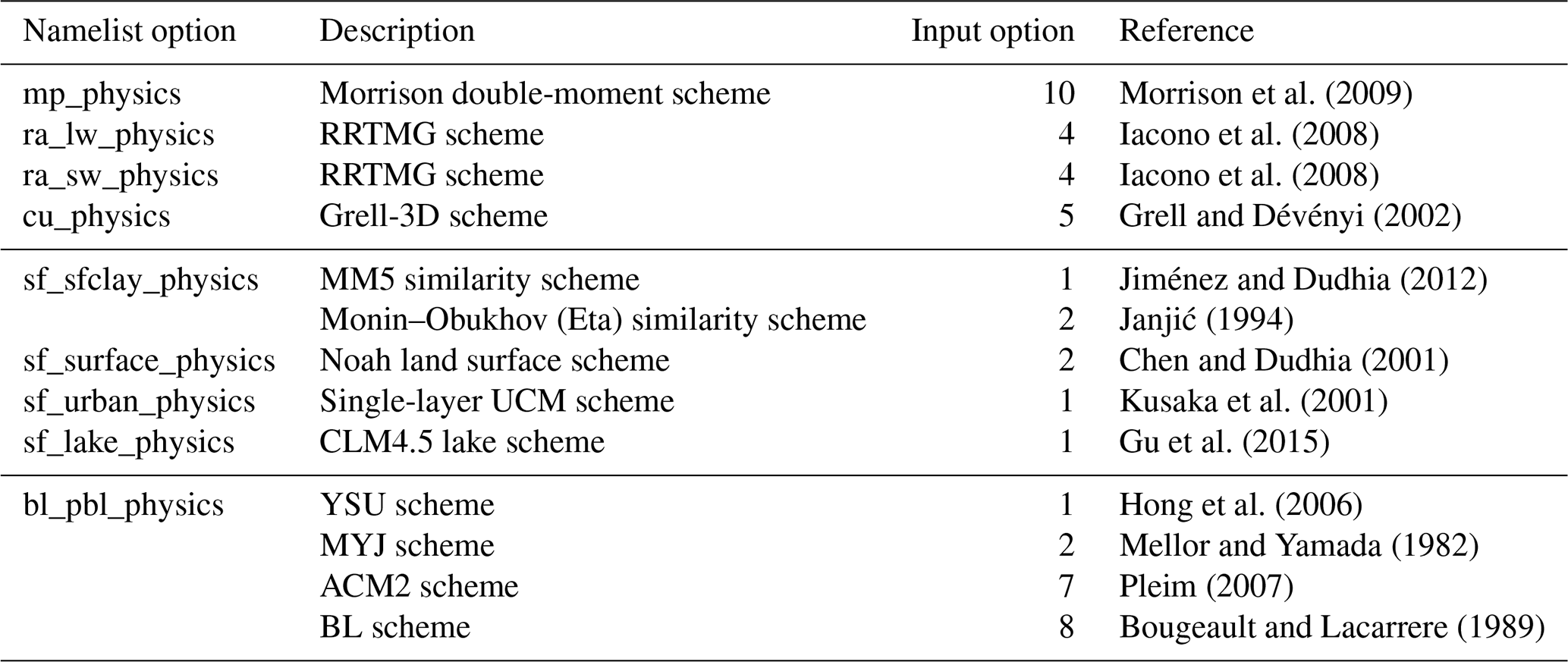
In this study, we adopt the model WRF-ARW (Advanced Research Weather Research and Forecasting) version 3.9.1 to evaluate the performance of PBL schemes. Long-term three-dimensional simulation experiments are conducted in 1 month of each season of 2016 (i.e., January, April, July, and October). Seven nested domains (D1, D2, D3, D4, D5, D6, and D7) are defined (Fig. 1a), with horizontal grid spacings of 75 km (74 × 74 grid cells, 9–59^∘ N, 61–146^∘ E), 15 km (281 × 281 grid cells, 13–51^∘ N, 77–136^∘ E), 3 km (331 × 331 grid cells, 34–44^∘ N, 111–124^∘ E), 3 km (316 × 356 grid cells, 26–34^∘ N, 114–126^∘ E), 3 km (331 × 331 grid cells, 25–33.5^∘ N, 100–110^∘ E), 3 km (236 × 301 grid cells, 18–25^∘ N, 110–119^∘ E), and 3 km (226 × 351 grid cells, 36–42.7^∘ N, 94–107^∘ E), respectively. Along the vertical direction, 48 vertical layers are configured blow the top, and the model top is set to 50 hPa. To resolve the PBL structure finely, 21 vertical layers are set below 2 km (i.e., the specific setting of vertical levels is σ=1.000, 0.997, 0.994, 0.991, 0.988, 0.985, 0.980, 0.975, 0.970, 0.960, 0.950, 0.940, 0.930, 0.920, 0.910, 0.895, 0.880, 0.865, 0.850, 0.825, 0.800). The initial and boundary conditions of meteorological fields are set up by using the NCEP Global Forecast System (GFS) Final (FNL) gridded analysis datasets, with a resolution of 1^∘ × 1^∘ (https://rda.ucar.edu/datasets/ds083.2/, last access: 4 August 2022). The Moderate Resolution Imaging Spectroradiometer (MODIS) dataset includes 20 land use categories (Broxton et al., 2014). The physical parameterization used in the present model is listed in Table 1.

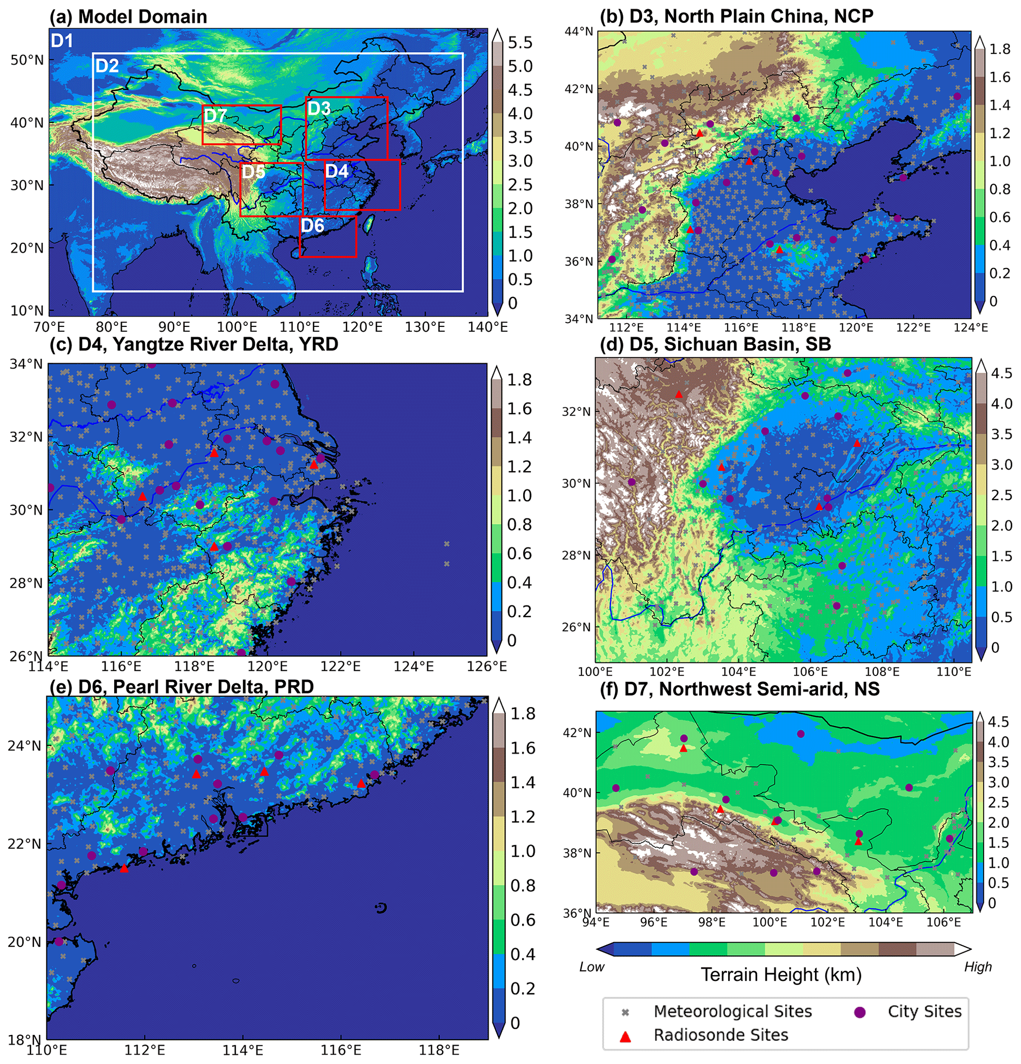
Figure 1 (a) Map of terrain height in the seven nested model domains. (b–f) Domains 3–7 correspond to the North Plain China (NCP), the Yangtze River Delta (YRD), the Sichuan Basin (SB), the Pearl River Delta (PRD) and the Northwest Semi-arid region (NS), respectively. The locations of surface meteorological stations and sounding stations are marked by the gray crosses and red triangles, respectively. The purple dots indicate the major city sites that are our main focus in each region.

Table 1 A brief description of the parameterization scheme in the model.

All simulations embodied a total of 16 months. The 40 h simulation is conducted beginning from 00:00 UTC of the previous day for each day (i.e., 492 simulation experiments), the first 16 h of each simulation is considered the spin-up period, and results obtained from the following 24 h simulations are analyzed for the present study.

2.3 Description of PBL parameterization schemes

2.3.1 YSU scheme

The YSU is a first-order nonlocal scheme with an explicit treatment entrainment process at the top of the PBL:

$$\begin{array}{}\text{(1)}& {\displaystyle \frac{\partial c}{\partial t}}={\displaystyle \frac{\partial }{\partial z}}\left[K_{\mathrm{c}}\left({\displaystyle \frac{\partial c}{\partial z}}-{\mathit{\gamma }}_{\mathrm{c}}\right)-\stackrel{\mathrm{‾}}{{\left(w^{\prime }{c}^{\prime }\right)}_{\mathrm{h}}}{\left({\displaystyle \frac{z}{h}}\right)}^{\mathrm{3}}\right],\end{array}$$

where c denotes u, v, and θ, and the ${\mathit{\gamma }}_{\mathrm{c}}=b\frac{\stackrel{\mathrm{‾}}{{\left(w^{\prime }{c}^{\prime }\right)}_{\mathrm{0}}}}{w_{\mathrm{s}\mathrm{0}}h}$ is the counter-gradient flux term, which increases the nonlocal effect due to the large-scale turbulence; z and h are the height of a level of the model and PBLH, respectively. The PBLH is defined by the bulk Richardson number method:

$$\begin{array}{}\text{(2)}& h=Ri{b}_{cr}{\displaystyle \frac{{\mathit{\theta }}_{\mathrm{va}}{\left|U\left(h\right)\right|}^{\mathrm{2}}}{g\left({\mathit{\theta }}_{\mathrm{v}}\left(h\right)-{\mathit{\theta }}_{\mathrm{s}}\right)}},\end{array}$$

where g is the gravity and Rib_cr is the critical bulk Richardson number, with a value of 0.25 under stable conditions and 0 under unstable conditions. θ_va is the virtual potential temperature at the lowest model level, θ_v(h) is the virtual potential temperature at h, and θ_s is the appropriate temperature near the surface (${\mathit{\theta }}_{\mathrm{s}}={\mathit{\theta }}_{\mathrm{va}}+{\mathit{\theta }}_T$, θ_T is the virtual temperature increment). Compared to the predecessor of the YSU scheme, the entrainment process is additionally treated explicitly (i.e., the last term on the right side of the Eq. 1).

Another key variable is K_c, which is the turbulent diffusion coefficient (TDC), and can be expressed based on the Monin–Obukhov similarity theory (MOST) as follows:

$$\begin{array}{}\text{(3)}& K_{\mathrm{c}}={\displaystyle \frac{\mathit{\kappa }{u}_{\ast }z}{{\mathit{\varphi }}_{\mathrm{c}}}}{\left(\mathrm{1}-{\displaystyle \frac{z}{h}}\right)}^{\mathrm{2}},\end{array}$$

where u_∗ is the surface frictional velocity and ϕ_c is dimensionless function, the expressions for different stability conditions are as follows.

• i.

  Unstable and neutral conditions.

  $$\begin{array}{}\text{(4a)}& {\displaystyle }{\mathit{\varphi }}_{\mathrm{m}}={\left(\mathrm{1}-\mathrm{16}{\displaystyle \frac{\mathrm{0.1}h}{L}}\right)}^{-\mathrm{1}/\mathrm{4}}\text{(4b)}& {\displaystyle }{\mathit{\varphi }}_{\mathrm{h}}={\left(\mathrm{1}-\mathrm{16}{\displaystyle \frac{\mathrm{0.1}h}{L}}\right)}^{-\mathrm{1}/\mathrm{2}}\end{array}$$
• ii.

  Stable conditions.

  $$\begin{array}{}\text{(4c)}& {\mathit{\varphi }}_{\mathrm{m}}={\mathit{\varphi }}_{\mathrm{h}}=\left(\mathrm{1}+\mathrm{5}{\displaystyle \frac{\mathrm{0.1}h}{L}}\right)\end{array}$$

  The TDC of momentum (i.e., K_m) is first calculated in the model, and then the TDC of heat (i.e., K_h) is calculated using the Prandtl number (i.e., $Pr=\frac{K_{\mathrm{m}}}{K_{\mathrm{h}}}$). The TDC controls the vertical mixing process of momentum and scalars within the PBL, and it is crucial that it is accurately described.

2.3.2 MYJ scheme

The MYJ scheme is a 1.5 order local closure scheme with a prognostic equation for turbulent kinetic energy (TKE, TKE $=e=\frac{\mathrm{1}}{\mathrm{2}}\left(u^{{}^{\prime }\mathrm{2}}+v^{{}^{\prime }\mathrm{2}}+w^{{}^{\prime }\mathrm{2}}\right))$:

$$\begin{array}{}\text{(5)}& \begin{array}{rl}{\displaystyle \frac{\partial \stackrel{\mathrm{‾}}{e}}{\partial t}}& =-{\displaystyle \frac{\mathrm{1}}{\stackrel{\mathrm{‾}}{\mathit{\rho }}}}{\displaystyle \frac{\partial }{\partial z}}\stackrel{\mathrm{‾}}{w^{\prime }{p}^{\prime }}-\stackrel{\mathrm{‾}}{w^{\prime }{u}^{\prime }}{\displaystyle \frac{\partial \stackrel{\mathrm{‾}}{u}}{\partial z}}-\stackrel{\mathrm{‾}}{w^{\prime }{v}^{\prime }}{\displaystyle \frac{\partial \stackrel{\mathrm{‾}}{v}}{\partial z}}\\ & -{\displaystyle \frac{\partial }{\partial z}}\stackrel{\mathrm{‾}}{w^{\prime }{e}^{\prime }}+{\displaystyle \frac{g}{{\mathit{\theta }}_{\mathrm{v}}}}\stackrel{\mathrm{‾}}{w^{\prime }{\mathit{\theta }}_{\mathrm{v}}^{\prime }}-\mathit{\epsilon }\end{array}.\end{array}$$

The first term on the right side of Eq. (5) is a pressure correlation term that describes TKE as being redistributed by pressure perturbations; the second and third terms are a shear production and loss terms, respectively; the fourth term represents the turbulent transport of TKE,; the fifth term describes the buoyant production and consumption term; and the sixth term represents viscous dissipation of TKE. To close the TKE equation, the turbulent fluxes must be parameterized. Based on the gradient transport theory (i.e., K theory), the turbulent fluxes can be indicated as follows:

$$\begin{array}{}\text{(6a)}& {\displaystyle }\stackrel{\mathrm{‾}}{w^{\prime }{u}^{\prime }}=-K_{\mathrm{m}}{\displaystyle \frac{\partial \stackrel{\mathrm{‾}}{u}}{\partial z}},\text{(6b)}& {\displaystyle }\stackrel{\mathrm{‾}}{w^{\prime }{v}^{\prime }}=-K_{\mathrm{m}}{\displaystyle \frac{\partial \stackrel{\mathrm{‾}}{v}}{\partial z}},\text{(6c)}& {\displaystyle }\stackrel{\mathrm{‾}}{w^{\prime }{\mathit{\theta }}^{\prime }}=-K_{\mathrm{h}}{\displaystyle \frac{\partial \stackrel{\mathrm{‾}}{\mathit{\theta }}}{\partial z}}.\end{array}$$

The TDC is proportional to the square root of TKE, and can be expressed as follows:

$$\begin{array}{}\text{(7a)}& {\displaystyle }{K}_{\mathrm{m}}=S_{\mathrm{m}}l{e}^{\mathrm{1}/\mathrm{2}},\text{(7b)}& {\displaystyle }{K}_{\mathrm{h}}=S_{\mathrm{h}}l{e}^{\mathrm{1}/\mathrm{2}},\end{array}$$

where l is mixing length and can be described as $l=\frac{l_{\mathrm{0}}\mathit{\kappa }z}{\mathit{\kappa }z+l_{\mathrm{0}}}$, where $l_{\mathrm{0}}=\mathit{\alpha }\frac{{\int }_{\mathrm{0}}^{\mathrm{\infty }}z{e}^{\mathrm{1}/\mathrm{2}}\mathrm{d}z}{{\int }_{\mathrm{0}}^{\mathrm{\infty }}{e}^{\mathrm{1}/\mathrm{2}}\mathrm{d}z}$ and α is an empirical constant (=0.1). When z converges to a very small value, l converges to κz. However, as z converges to a very large value, l converges to l₀.

To obtain the S_m and S_h in Eq. (7), G_m and G_h are defined as follows:

$$\begin{array}{}\text{(8a)}& {\displaystyle }{G}_{\mathrm{m}}={\displaystyle \frac{l^{\mathrm{2}}}{\mathrm{2}e}}\left[{\left({\displaystyle \frac{\partial \stackrel{\mathrm{‾}}{u}}{\partial z}}\right)}^{\mathrm{2}}+{\left({\displaystyle \frac{\partial \stackrel{\mathrm{‾}}{v}}{\partial z}}\right)}^{\mathrm{2}}\right],\text{(8b)}& {\displaystyle }{G}_{\mathrm{h}}=-{\displaystyle \frac{l^{\mathrm{2}}}{\mathrm{2}e}}{\displaystyle \frac{g}{{\mathit{\theta }}_{\mathrm{v}}}}{\displaystyle \frac{\partial {\mathit{\theta }}_{\mathrm{v}}}{\partial z}}.\end{array}$$

S_m and S_h are functions of G_m and G_h, and can be denoted as follows:

$$\begin{array}{}\text{(9a)}& {\displaystyle }\begin{array}{rl}& S_{\mathrm{m}}\left(\mathrm{6}{A}_{\mathrm{1}}{A}_{\mathrm{2}}{G}_{\mathrm{m}}\right)+S_{\mathrm{h}}\left(\mathrm{1}-\mathrm{3}{A}_{\mathrm{2}}{B}_{\mathrm{2}}{G}_{\mathrm{h}}-\mathrm{12}{A}_{\mathrm{1}}{A}_{\mathrm{2}}{G}_{\mathrm{h}}\right)\\ & =A_{\mathrm{2}}\end{array},\text{(9b)}& {\displaystyle }\begin{array}{rl}& A_{\mathrm{1}}\left(\mathrm{1}+\mathrm{6}{A}_{\mathrm{1}}^{\mathrm{2}}{G}_{\mathrm{m}}-\mathrm{9}{A}_{\mathrm{1}}{A}_{\mathrm{2}}{G}_{\mathrm{h}}\right)\\ & -S_{\mathrm{h}}\left(\mathrm{12}{A}_{\mathrm{1}}^{\mathrm{2}}{G}_{\mathrm{h}}+\mathrm{9}{A}_{\mathrm{1}}{A}_{\mathrm{2}}{G}_{\mathrm{h}}\right)=A_{\mathrm{1}}\left(\mathrm{1}-\mathrm{3}{C}_{\mathrm{1}}\right)\end{array},\end{array}$$

where $\left[A_{\mathrm{1}},A_{\mathrm{2}},B_{\mathrm{1}},B_{\mathrm{2}},C_{\mathrm{1}}\right]=\left[\mathrm{0.660},\mathrm{0.657},\mathrm{11.878},\mathrm{7.227},\mathrm{0.001}\right]$.

The PBLH in the MYJ scheme is defined as the height at which the TKE is reduced to a critical value of 0.1 m² s⁻².

2.3.3 ACM2 scheme

Unlike the YSU scheme, the ACM2 scheme applies the transilient matrix to deal with the contribution of nonlocal fluxes. The governing equation can be expressed as follows:

$$\begin{array}{}\text{(10)}& \begin{array}{rl}{\displaystyle \frac{\partial C_i}{\partial t}}& =f_{\mathrm{conv}}\mathrm{Mu}{C}_{\mathrm{1}}-f_{\mathrm{conv}}{\mathrm{Md}}_i{C}_i\\ & +f_{\mathrm{conv}}{\mathrm{Md}}_{i+\mathrm{1}}{C}_{i+\mathrm{1}}{\displaystyle \frac{\mathrm{\Delta }{z}_{i+\mathrm{1}}}{\mathrm{\Delta }{z}_i}}\\ & +{\displaystyle \frac{\partial }{\partial z}}\left[K_{\mathrm{c}}\left(\mathrm{1}-f_{\mathrm{conv}}\right){\displaystyle \frac{\partial C_i}{\partial z}}\right]\end{array}.\end{array}$$

The first three terms on the right side of Eq. (10) represent the nonlocal mixing effect, and the fourth term represents the local mixing effect. Here, C_i is the variable at layer i, Mu is the nonlocal upward convective mixing rate, Md_i is the downward mixing rate from layer i to layer i−1, Δz_i is the thickness of layer i, and C₁ represents the variable at the lowest layer in the model. f_conv is the weighting factor for the nonlocal and local effects (i.e., $f_{\mathrm{conv}}=\frac{K_{\mathrm{h}}{\mathit{\gamma }}_{\mathrm{h}}}{K_{\mathrm{h}}{\mathit{\gamma }}_{\mathrm{h}}-K_{\mathrm{h}}\frac{\partial \mathit{\theta }}{\partial z}}$), where the value of f_conv ranges from 0 to 1, a larger f_conv indicates stronger nonlocal mixing.

There are two methods to calculate the TDC, and the first method is the same as the YSU scheme, i.e., Eq. (3), but there is also a very stable condition in the ACM2 scheme. In this case, the dimensionless function can be expressed as ${\mathit{\varphi }}_{\mathrm{m}}={\mathit{\varphi }}_{\mathrm{h}}=\left(\mathrm{5}+\frac{\mathrm{0.1}h}{L}\right)$.

The second calculation principle is based on the mixing length theory, which uses mixing length and stability function to calculate TDC:

$$\begin{array}{}\text{(11)}& K_{\mathrm{h}}=\mathrm{0.01}+l^{\mathrm{2}}\sqrt{\mathrm{ss}}{f}_{\mathrm{h}}\left(Ri\right),\end{array}$$

where l is similar to the MYJ scheme, but l₀ is a constant (=80), ss is the wind shear ($\mathrm{ss}={\left(\partial \stackrel{\mathrm{‾}}{u}/\partial z\right)}^{\mathrm{2}}+{\left(\partial \stackrel{\mathrm{‾}}{v}/\partial z\right)}^{\mathrm{2}})$, 0.01 denotes the minimum value of the TDC in the model, and f_h(Ri) is the empirical stability functions of gradient Richardson number of heat.

• i.

  when Ri≥0:

  $$\begin{array}{}\text{(12a)}& f_{\mathrm{h}}\left(Ri\right)={\left(\mathrm{1}-\mathrm{25}Ri\right)}^{\mathrm{1}/\mathrm{2}}\end{array}$$
• ii.

  when Ri<0:

  $$\begin{array}{}\text{(12b)}& \begin{array}{rl}{f}_{\mathrm{h}}\left(Ri\right)& ={\displaystyle \frac{\mathrm{1}}{\mathrm{1}+\mathrm{10}Ri+\mathrm{50}R{i}^{\mathrm{2}}+\mathrm{5000}R{i}^{\mathrm{4}}}}\\ & +\mathrm{0.0012}\end{array}\end{array}$$

Similarly, the empirical stability functions of momentum can be indicated as follows.

• i.

  when Ri≥0:

  $$\begin{array}{}\text{(13a)}& K_{\mathrm{m}}=Pr\cdot K_{\mathrm{h}}\end{array}$$
• ii.

  when Ri<0:

  $$\begin{array}{}\text{(13b)}& {\displaystyle }{f}_{\mathrm{m}}\left(Ri\right)=Pr\cdot f_{\mathrm{h}}\left(Ri\right)+\mathrm{0.00104}\text{(13c)}& {\displaystyle }{K}_{\mathrm{m}}=\mathrm{0.01}+l^{\mathrm{2}}\sqrt{\mathrm{ss}}{f}_{\mathrm{m}}\left(Ri\right)\end{array}$$

The ACM2 scheme has a range setting for the TDC in the model with a minimum value of 0.01 m² s⁻² and a maximum value that cannot exceed 1000 m² s⁻².

The PBLH discrimination in the ACM2 scheme is similar to the YSU scheme and is defined with the bulk Richardson number method. The difference is that the entrainment region at the top of the PBL is considered in the ACM2 scheme and turbulence still exists due to the wind shear and thermal penetration. Therefore, special processing of the PBLH is required under unstable and stable conditions.

2.3.4 BL scheme

The BL scheme is also a 1.5 order local closure scheme, and the TDC is calculated in a similar way to Eq. (7) of the MYJ scheme. Nevertheless, the function S_m and mixing length (i.e., l) are different from the MYJ scheme. In the BL scheme, S_m is a constant 0.4, and the l is divided into upward and downward mixing length (i.e., l_up and l_down), which are defined as follows:

$$\begin{array}{}\text{(14a)}& {\displaystyle }\underset{z}{\overset{z+l_{\mathrm{up}}}{\int }}\mathit{\beta }\left[\mathit{\theta }\left(z\right)-\mathit{\theta }\left(z^{\prime }\right)\right]\mathrm{d}{z}^{\prime }=e\left(z\right),\text{(14b)}& {\displaystyle }\underset{z-l_{\mathrm{down}}}{\overset{z}{\int }}\mathit{\beta }\left[\mathit{\theta }\left(z^{\prime }\right)-\mathit{\theta }\left(z\right)\right]\mathrm{d}{z}^{\prime }=e\left(z\right),\end{array}$$

where β is the buoyancy coefficient and the l is equal to the minimum of l_up and l_down (i.e., $l=min\left(l_{\mathrm{up}},l_{\mathrm{down}}\right))$. It is worth noting that in the BL scheme the TDC of heat is equal to the TDC of momentum (i.e., K_h=K_m). In addition, the PBLH of the BL scheme is defined as the height at which the virtual potential temperature of a layer is greater than that of the first layer by 0.5 K.

To accommodate different methods of calculating PBLH for different schemes and to evaluate the simulation performance of PBLH, two methods are employed to calculate PBLH using observed data in this study, the first being the bulk Richardson number method, and the detailed calculation principle is as follows (Miao et al., 2018):

$$\begin{array}{}\text{(15)}& Ri\left(z\right)={\displaystyle \frac{\left(g/{\mathit{\theta }}_{\mathrm{s}}\right)\left({\mathit{\theta }}_z-{\mathit{\theta }}_{\mathrm{s}}\right)\left(z-z_{\mathrm{s}}\right)}{{\left(u_z-u_{\mathrm{s}}\right)}^{\mathrm{2}}+{\left(v_z-v_{\mathrm{s}}\right)}^{\mathrm{2}}+b{u}_{\ast }^{\mathrm{2}}}}\end{array}$$

where z is the height, g is the gravity, θ is the virtual potential temperature, u and v are the components of the horizontal wind, b is a constant, and u_∗ is the friction velocity. The subscript “s” indicates the near surface. Since the friction velocity is much smaller in magnitude than the wind shear, the b is set to 0, ignoring the effect of surface friction (Vogelezang and Holtslag, 1996; Seidel et al., 2012). The PBLH is estimated as the lowest layer height when Ri reaches a critical value of 0.25.

The second method adopts the same calculation method as the BL scheme, i.e., the virtual potential temperature method:

$$\begin{array}{}\text{(16)}& \mathrm{\Delta }{\mathit{\theta }}_{v\mathrm{|}\mathrm{PBLH}}={\mathit{\theta }}_{v\mathrm{1}}+\mathrm{0.5}.\end{array}$$

The PBLH is the height when the virtual potential temperature exceeds the virtual potential temperature of the first level by 0.5 K.

2.4 Evaluation of the model

To evaluate the PBL schemes and the performance of the model for estimating meteorological variables, the statistical parameters used in this statistical analysis are defined as follows (Emery et al., 2017).

Index of agreement (IOA):

$$\begin{array}{}\text{(17)}& \mathrm{IOA}=\mathrm{1}-{\displaystyle \frac{\left[\sum _{i=\mathrm{1}}^n\mathrm{|}{X}_{\mathrm{sim},i}-X_{\mathrm{obs},i}{\mathrm{|}}^{\mathrm{2}}\right]}{\left[\sum _{i=\mathrm{1}}^n{\left(\mathrm{|}{X}_{\mathrm{sim},i}-\stackrel{\mathrm{‾}}{X_{\mathrm{obs}}}\mathrm{|}+\mathrm{|}{X}_{\mathrm{obs},i}-\stackrel{\mathrm{‾}}{X_{\mathrm{obs}}}\mathrm{|}\right)}^{\mathrm{2}}\right]}}\end{array}$$

Mean bias (MB):

$$\begin{array}{}\text{(18)}& \mathrm{MB}={\displaystyle \frac{\mathrm{1}}{n}}\sum _{i=\mathrm{1}}^n\left(X_{\mathrm{sim},i}-X_{\mathrm{obs},i}\right)\end{array}$$

Root-mean-square error (RMSE):

$$\begin{array}{}\text{(19)}& \mathrm{RMSE}=\sqrt{{\displaystyle \frac{\mathrm{1}}{n}}\sum _{i=\mathrm{1}}^n{\left(X_{\mathrm{sim},i}-X_{\mathrm{obs},i}\right)}^{\mathrm{2}}}\end{array}$$

Normalized standard deviations (NSD):

$$\begin{array}{}\text{(20)}& \mathrm{NSD}={\displaystyle \frac{\sqrt{\frac{\mathrm{1}}{n-\mathrm{1}}\sum _{i=\mathrm{1}}^n{\left(X_{\mathrm{sim},i}-\stackrel{\mathrm{‾}}{X_{\mathrm{sim}}}\right)}^{\mathrm{2}}}}{\sqrt{\frac{\mathrm{1}}{n-\mathrm{1}}\sum _{i=\mathrm{1}}^n{\left(X_{\mathrm{obs},i}-\stackrel{\mathrm{‾}}{X_{\mathrm{obs}}}\right)}^{\mathrm{2}}}}}\end{array}$$

Relative bias (RB):

$$\begin{array}{}\text{(21)}& \mathrm{RB}={\displaystyle \frac{\stackrel{\mathrm{‾}}{X_{\mathrm{sim}}}-\stackrel{\mathrm{‾}}{X_{\mathrm{obs}}}}{\stackrel{\mathrm{‾}}{X_{\mathrm{obs}}}}}\times \mathrm{100}\mathit{\%}\end{array}$$

Here X_sim,i and X_sim,i represent the value of simulation and observation, respectively; i refers to time; and n is the total number of time series. $\stackrel{\mathrm{‾}}{X_{\mathrm{sim}}}$ and $\stackrel{\mathrm{‾}}{X_{\mathrm{obs}}}$represent the average simulation and observation.

The Taylor diagram is a compact tool that simultaneously displays the values of four statistical parameters: IOA, NSD, RB, and RMSE. In particular, in these diagrams the perfect match of a model with the observations would be the point with IOA of 1, NSD of 1, RB of 0, and RMSE of 0.

3 Results and discussion

In Sect. 3.1, the mechanistic analysis of the PBL schemes for the simulation of near-surface meteorological parameters, including 2 m temperature, 2 m relative humidity, and 10 m wind speed and direction. Section 3.2 gives an in-depth analysis of different schemes for PBL vertical structures. In Sect. 3.3, the PBLH was evaluated for different schemes. In Sect. 3.4, the reason for the differences in turbulent diffusion are interrogated from the calculation principle of the schemes. Section 3.5 summarizes the performance and expressiveness of different PBL schemes in different regions and recommends the optimal choice of PBL scheme.

3.1 Surface meteorological variables

3.1.1 The 2 m temperature and relative humidity

To better analyze the variation in the time series, we selected representative stations in different regions. Figure 2 shows the diurnal variation in 2 m temperature (i.e., T₂) for 4 months (i.e., January, April, July, and October 2016) at representative sites (indicated in the purple dots in Fig. 1) in the five regions. The model basically captures the daily variation characteristics of T₂, but there are significant differences between different regions and seasons. The simulated results for July are closest to the observed values (Fig. 2c1–c5) anywhere. Overall, the mean biases (MBs) of the diurnal variation in T₂ predicted in July for the NCP, YRD, SB, PRD, and NS regions are 0.61–1.19, −0.02 to −0.56, −0.32 to −0.60, −0.38 to −0.69, and 0.28–0.81^∘, respectively. However, a smaller value of the mean bias does not mean that the simulated value of the model is closer to the observed value. For example, if one overestimation and the other underestimation occur during the day and night, the average results will cancel each other out, resulting in a small mean bias. Accordingly, more statistical parameters are needed to further evaluate the optimal scheme. In the other 3 months (January, April, and October), the simulated results of T₂ are overestimated to varying degrees during daytime in the YRD, SB, and PRD regions, while in the NS region, T₂ are underestimated to varying degrees (Fig. 2a2–b5, d2–d5 and Table 1). In the NCP regions, T₂ presents underestimation in January by the model with the YSU, ACM2, BL, and MYJ schemes are −1.33, −1.21, −0.52, and −1.18^∘, respectively, while overestimation arises in the other 3 months (Table 1). In the five regions, the simulation results of the nighttime T₂ outperform those of the daytime T₂ for almost 4 months. At night, the MYJ scheme shows a significant underestimation of T₂ for all months in five regions compared to the other three schemes (Fig. 2 and Table 1). The simulation results of Hu et al. (2010) and Xie et al. (2012) have also obtained the lowest temperature for the MYJ scheme during the nighttime.

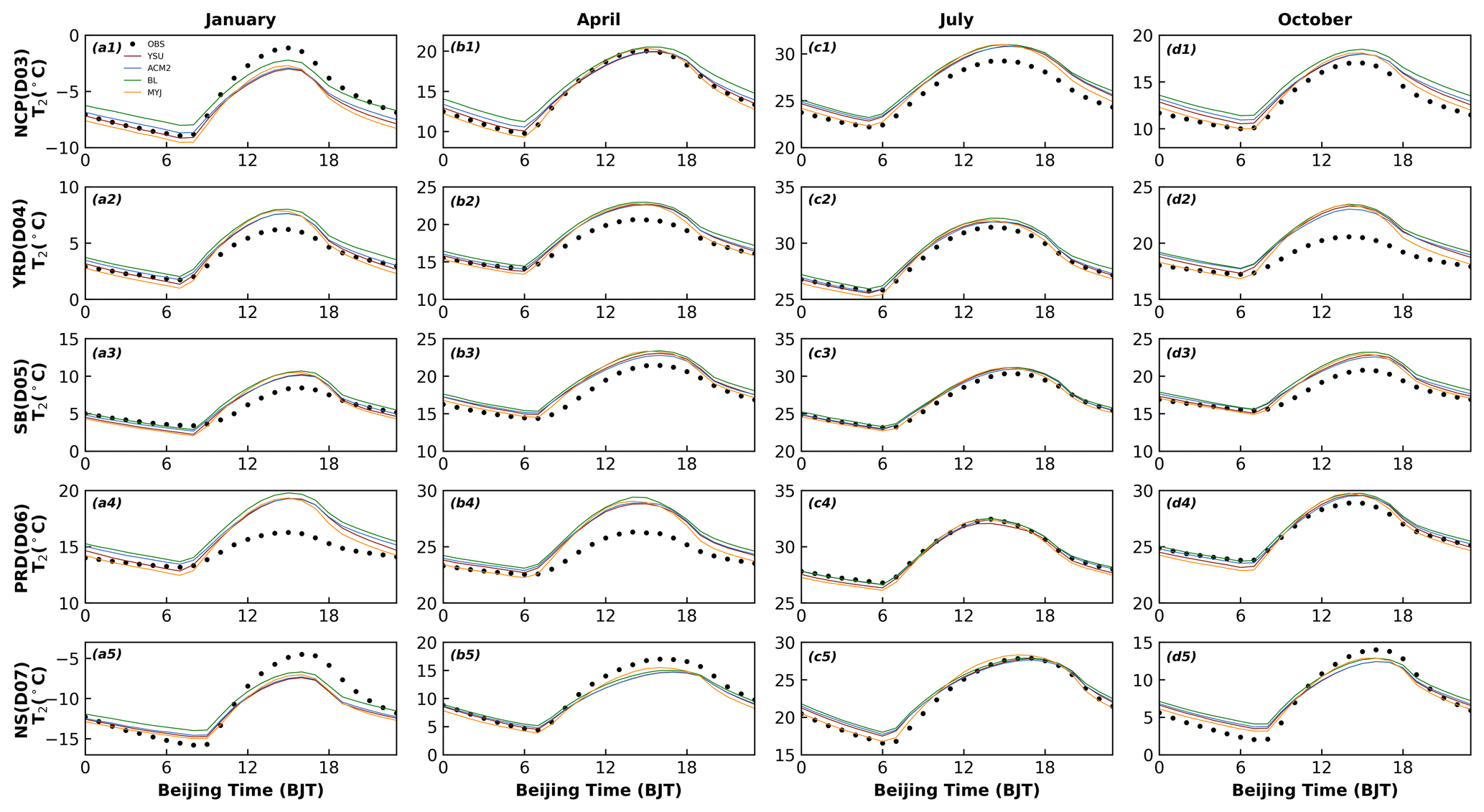
Figure 2 Time series of diurnal variation in observed and simulated 2 m temperature in five regions for four seasons.

The 2 m temperature does not actually represent the air temperature at a height of 2 m, but it is a diagnostic variable of the near-surface temperature. It is calculated from the surface temperature (T_s), the sensible heat flux (HFX) and the heat transfer coefficient (C_h). The T_s is a prognostic variable, which is obtained in the model through the energy balance equation:

$$\begin{array}{}\text{(22)}& \left(\mathrm{1}-\mathit{\alpha }\right)S\downarrow +L\downarrow -L\uparrow +G-HFX-LH=\mathrm{0},\end{array}$$

where α is the albedo of the underlying surface, S↓ represents the downward of the shortwave radiation, L↓ is the downward of the longwave radiation emitted by the cloud and atmosphere, L↑ is the upward of the longwave emitted by the ground surface, G is the ground heat flux and is positive when heat transfers from the soil to the near surface, HFX is the sensible heat flux, and LH is the latent heat flux.

We compare the effects of the six variables mentioned above on T_s with the expectation that we can further examine the reasons for the differences in T₂ variation between different schemes. The YSU scheme is used as a control and analyzed in comparison with each of the schemes.

The nonlocal closure scheme (YSU) and the local closure scheme (MYJ) are compared first. Theoretically, the greater the downward shortwave radiation (S↓) becomes, the more energy reaches the ground, and the higher the surface temperature (T_s) is. After comparing the YSU and MYJ schemes, the surface temperature does not show a proportional change with the downward shortwave radiation, and the S↓ of the MYJ scheme is almost the same as that of the YSU scheme (Fig. 3a1–e1), but the T_s of the MYJ scheme is the lowest (Fig. 4a1–e1). Therefore, the S↓ is not the main factor that causes the difference in T_s between the two schemes. There is no significant difference in the upward or downward longwave radiation between these two schemes (Fig. 3a2–e3), so the effect of longwave radiation on the T_s can also be excluded. During the daytime, the MYJ scheme transfers less heat from the surface to the soil than the YSU scheme (Fig. 3a4–e4), and the T_s of the MYJ scheme should be higher than that of the YSU scheme. But that is not how it has turned out (Fig. 4a1–e1). Thus, the ground heat flux (G) is also not a key factor that directly affects the T_s. The latent heat flux (LH) is mainly related to water vapor (or relative humidity), so further attention is paid to the effect of sensible heat flux (HFX) on T_s (Fig. 3a5–e6). The HFX is determined by the difference between the surface temperature and the 2 m temperature (T_s−T₂), and the heat transfer coefficient (C_h) ($HFX=\mathit{\rho }{C}_{\mathrm{h}}{u}_{\mathrm{1}}\left(T_{\mathrm{s}}-T_{\mathrm{2}}\right)$; here, ρ is the air density, u₁ is the wind speed at the first level of the model). MYJ has the largest HFX and transfers more heat from the surface to the atmosphere, resulting in the largest energy loss at the surface, which should correspond to the smallest T_s (Figs. 3a6–e6, 4a1–e1). The smallest difference between the two temperatures indicates a smaller temperature gradient and more uniform mixing, symbolizing the largest C_h, which is also true (Fig. 4a2–e3). A larger C_h would lead to higher T₂ during the day. Although the T_s of the MYJ scheme is significantly lower than YSU scheme, it makes the T₂ higher due to the large C_h. During the daytime, less heat is transferred from the surface to the soil in the MYJ scheme, which results in lower soil temperature. During the nighttime, the difference in HFX and temperature gradient between the two schemes decreases, and the lower soil temperature results in lower T_s and T₂.

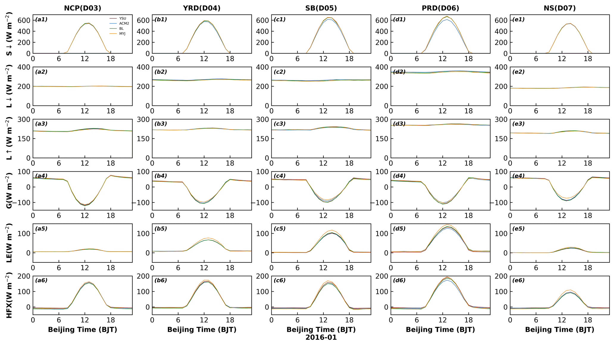
Figure 3 Time series of diurnal variation in (a1–e1) downward shortwave radiation (S↓), (a2–e2) downward longwave radiation (L↓), (a3–e3) upward longwave radiation (L↑), (a4–e4) ground heat flux (G), (a5–e5) latent heat flux (LH), and (a6–e6) sensible heat flux (HFX) by four PBL schemes in five regions in January.

The differences between the YSU scheme and the ACM2 scheme are further explored. Except for the NCP and NS regions, the S↓ of the ACM2 scheme is smaller than that of the YSU scheme in the other three regions (i.e., YRD, SB, and PRD) (Fig. 3b1–d1). The HFX of the ACM2 scheme is smaller than that of the YSU scheme (Fig. 3b6–d6), the heat loss from the surface of the ACM2 scheme is lower, and the T_s of the ACM2 scheme should be higher. However, the T_s corresponding to the ACM2 scheme is lower than that of the YSU scheme (Fig. 4b1–d1), reflecting that the S↓ varies proportionally with the T_s, and it is the main factor controlling the T_s variation. In the ideal case, assuming the same temperature gradient for the nonlocal schemes, the T₂ of the YSU scheme should also be higher than that of the ACM2 scheme when the T_s of the YSU scheme is higher than that of the ACM2 scheme with the same C_h. However, it can be seen that the C_h of the ACM2 scheme and YSU scheme are the same (Fig. 4b2–d2), and the temperature gradient of the YSU scheme is greater than that of ACM2 scheme (Fig. 4b3–d3). The T₂ of the ACM2 scheme should be slightly higher than the ideal case, closer to the T₂ of the YSU scheme, and it may even also exceed T₂ of the YSU scheme. At night, the T_s of the YSU scheme is lower than that of the ACM2 scheme, and the C_h of the YSU scheme is smaller than that of the ACM2 scheme (Fig. 4a1–e2). Meanwhile, the difference in HFX between the two schemes is not obvious at night, contributing to lower T₂ of the YSU scheme. In both NCP and NS regions, there is no significant difference in downward shortwave radiation between two schemes, and no noticeable difference between T₂ and T_s.

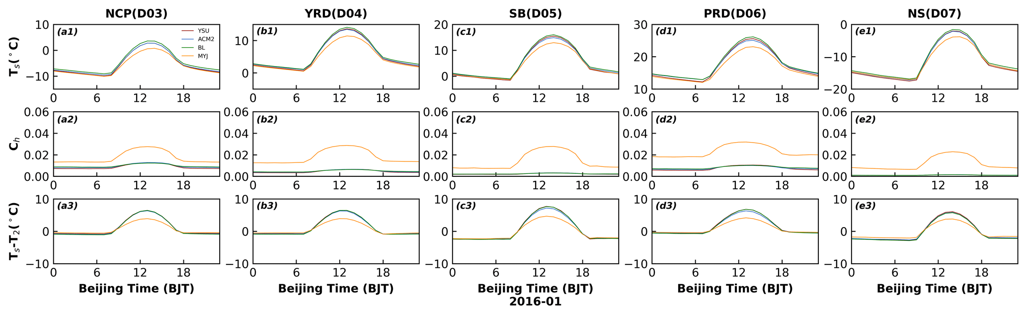
Figure 4 Time series of diurnal variation in (a1–e1) surface temperature (T_s) and (a2–e2) heat transfer coefficient (C_h) and (a3–e3) the difference between the surface temperature and the 2 m temperature (T_s−T₂) of four PBL schemes in five regions in January (winter).

Following this, the reasons for the simulated temperature difference between the YSU scheme and the BL scheme are demonstrated. During the daytime, the S↓ of both schemes is the same (Fig. 3a1–e1), but the HFX of the BL scheme is smaller than that of the YSU scheme (Fig. 3a6–e6), less heat is loss at the surface, hence the T_s should be higher than that of the YSU scheme (Fig. 4a1–e1). The C_h of both schemes are the same; thus, the BL scheme has a higher T₂ (Figs. 2, 4a1–e2). At night, the HFX of BL scheme is larger than that of YSU scheme, more heat is transferred from atmosphere to the surface, and the larger C_h results in higher T₂ (Figs. 3a6–e6, 4a1–e2).

Finally, we can also uncover the reasons for the difference between the local closure schemes (MYJ and BL). The larger HFX of the MYJ scheme leads to a lower T_s in the daytime, while the temperature gradient of MYJ scheme is smaller than that of the BL scheme, and C_h is larger than BL scheme (Figs. 3a6–e6, 4). Therefore, the difference in T₂ between the two schemes is smaller than that in T_s. The T₂ of the MYJ scheme is closer to that of the BL scheme.

In conclusion, the causes of temperature differences simulated by the nonlocal closure schemes should first focus on the effect of the downward shortwave radiation (S↓), and when it comes to the local closure scheme, the effect of HFX should be further concerned. All of the above results have been analyzed for January 2016, and the results for the other 3 months are similar (Figs. S1–S6 in the Supplement).

The results for the months of January, April, and October differ slightly from those of July. In terms of regional distribution differences, T₂ in the northern and near-mountainous regions of the NCP region is significantly underestimated in the daytime for January, April, and October, while T₂ in other areas of the NCP region shows an overestimation (Figs. 5, S7, S8a1–e1). The range of overestimated areas is smaller than the underestimated area in January and is only present in a small part of the area south of Hebei and Shandong provinces (Fig. 5a1–e1). The relative bias (RB) of the underestimated (overestimated) T₂ with the YSU, ACM2, BL, and MYJ schemes is −0.60 % (0.15 %), −0.57 % (0.17 %), −0.43 % (0.26 %) and −0.60 % (0.20 %), respectively, in January. In these 3 months, temperature is also overestimated at almost all stations in the YRD region (RB = 0.38 %–0.50 % in January, RB = 0.49 %–0.65 % in April, and RB = 0.58 %–0.70 % in October) and underestimated at some stations along the coast (RB = −0.13 % to −0.24 % in January, RB = −0.32 % to −0.37 % in April, and RB = −0.23 % to −0.28 % in October) (Figs. 5, S7, S8a2–e2). The results show an overestimation of T₂ simulated in those stations in the basin for the SB region and the simulation results of the stations in the plain for the NCP region, while for the stations in the hilltop areas, the T₂ shows an underestimation (Figs. 5, S7, S8a3–e3). In the PRD region, the entire region exhibits an overestimation of T₂, with the simulation results in October (RB = 0.06 %–0.15 %) being significantly better than those in January (RB = 0.59 %–0.81 %) and April (RB = 0.56 %–0.67 %), with a lower degree of T₂ overestimation (Figs. 5, S7, S8a4–e4). The BL scheme simulates a higher T₂ and a large range of overestimated areas (about 167, 378, 252, and 100 stations in the NCP, YRD, SB, and PRD regions, respectively). The NS region has a more complex topography and higher elevation, and the T₂ is underestimated at almost all stations, with the best simulation results being in October (RB = −0.04 % to −0.21 %) and worst being in April (RB = −0.49 % to −0.64 %).

For July, the simulation results are significantly different from the other 3 months. The relative bias of T₂ simulated with the YSU, ACM2, BL, and MYJ schemes are 0.47 %, 0.46 %, 0.53 %, and 0.46 %, respectively, in the NCP region. The overestimation results are similar to daytime, with the most pronounced overestimation for the BL scheme. For the southern region of the NCP, the T₂ is consistently overestimated regardless of the season (Fig. S9a1–e1). The T₂ at most stations is underestimated in the YRD region, which is different from the other 3 months (Fig. S9a2–e2). In summer, the temperature of the ocean, affected by the subtropical high (prevailing southeasterly winds), is lower than that of the land, and the transport of momentum is accompanied by the transport of heat from the sea to the land, causing the temperature of the land to decrease. The T₂ of the basin area in the SB region is well reproduced, and no significant overestimation occurs (Fig. S9a3–e3). There is an underestimation of the T₂ at most stations in the PRD region (but to a lesser extent) (Fig. S9a4–e4). In contrast, for the NS region, the temperature is overestimated for areas at lower elevations and underestimated (or better reproduced) for areas at higher elevations (Fig. S9a5–e5).

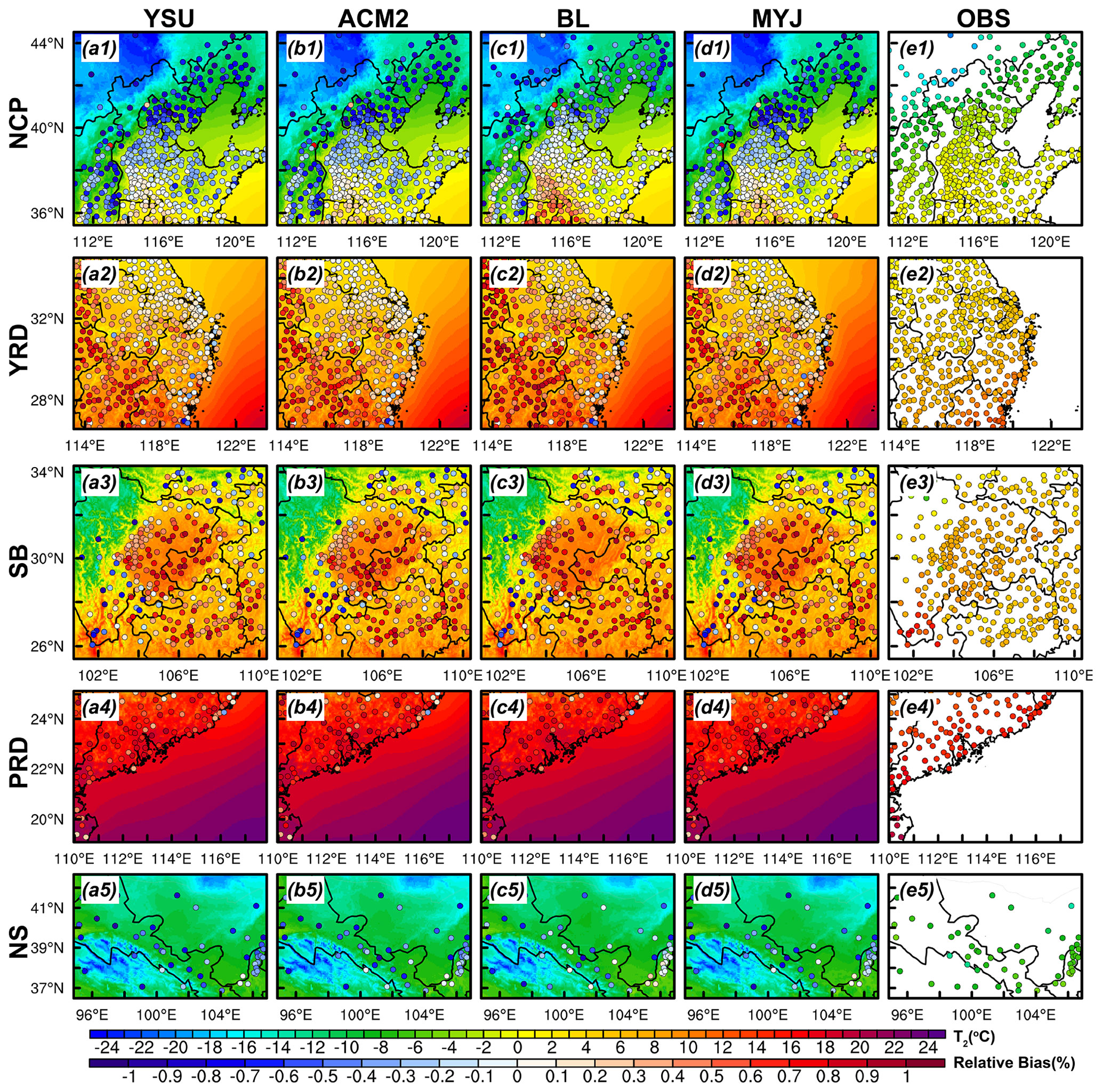
Figure 5 Regional distribution of 2 m temperature simulated by (a-d) four PBL schemes in five regions during the daytime in January (winter), (e1–e5) distribution of observation in five regions, and (a1–d5) distribution of relative bias between simulations and observations is denoted by scatters.

The relative deviation of the nighttime T₂ simulations is less than that of the daytime, regardless of the region and month (Figs. 6, S10–S12). The differences between the four schemes are more striking at night compared to the daytime. The BL scheme simulates the highest T₂ and the MYJ scheme simulates the lowest T₂ in the whole region (Figs. 6, S10–S12). Compared to the observed values, the MYJ scheme is the best when all schemes overestimate the simulated temperature, but if there is an underestimation, the MYJ scheme is no longer the best scheme. Later, a comprehensive statistical evaluation of the schemes will be presented. For the NCP region, the overestimation and underestimation in the whole region do not show a north–south divide (or a mountain–plain divide) as in the daytime (Figs. 5, 6a1–e1). In the YRD region, the temperature along the coastal area still shows a significant underestimation (Figs. 6, S10–S12a2–e2). Similar to the daytime, the temperature at stations in the hilltop areas of the SB region still present an underestimation (Figs. 6, S10–S12a3–e3). Most stations show the underestimation of T₂ in July and October in the PRD region (Figs. S11–S12a4–e4). In the NS region, the relative deviation of temperature simulations in October is greater than that in daytime (RB = 0.17 %–0.56 %) (Figs. 5, S12a5–e5).

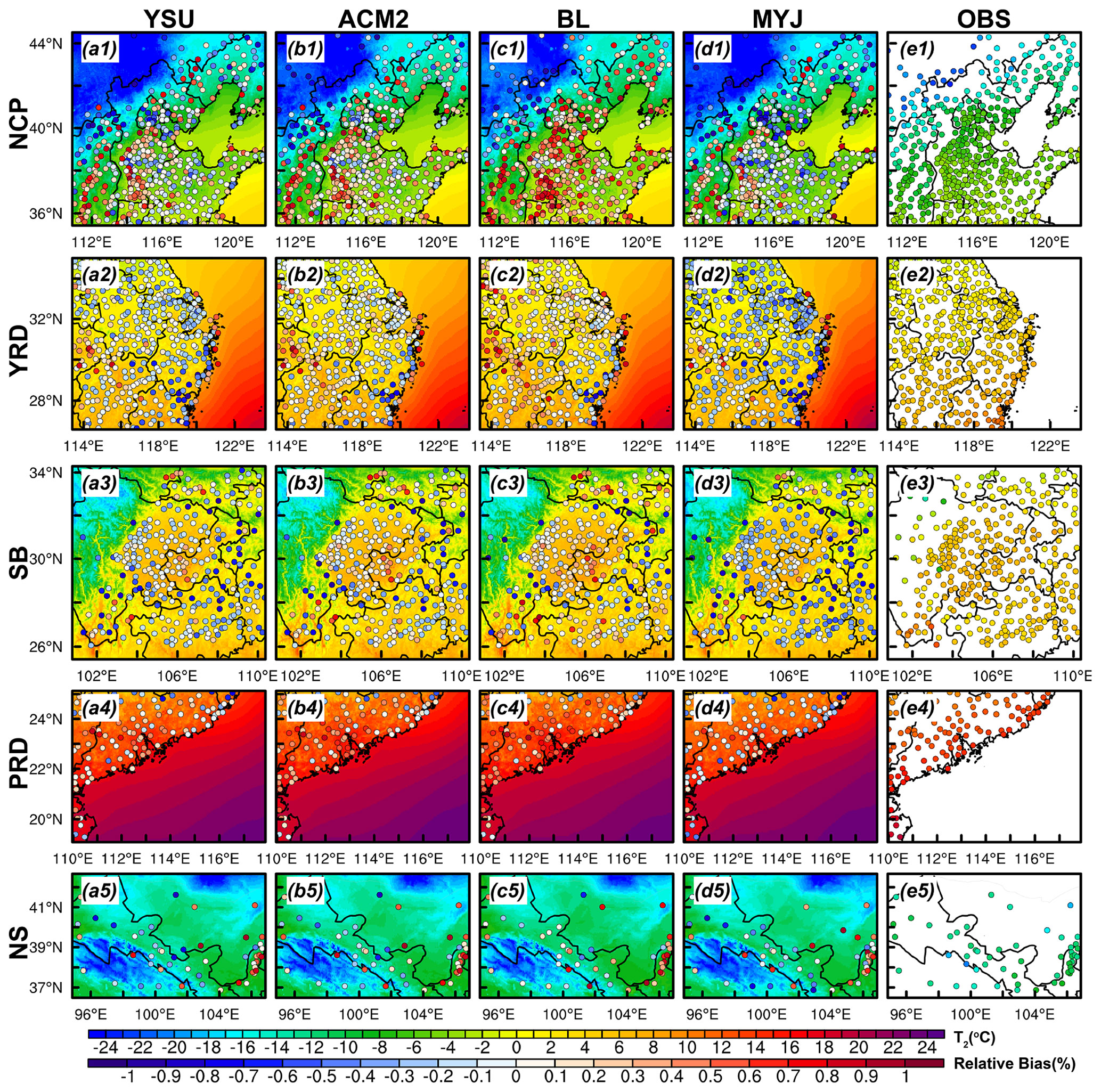
Figure 6 Similar to Fig. 5 but at night.

In summary, the simulation results of T₂ have the following main characteristics. From the perspective of differences between observations and simulations, (1) the simulation results for July are better compared to the other 3 months. (2) The simulation results at night are better than those at daytime, with less relative deviation, especially in winter (i.e., January and October). (3) The temperature is easily underestimated at higher altitudes and overestimated in plains and basin areas. From the perspective of the differences between the different schemes, (1) the differences in the performance of the four schemes are more noticeable at night. (2) The difference in the simulation of temperature in the nonlocal closure schemes is mainly attributed to the difference in downward shortwave radiation (S↓), and the difference in the variation in sensible heat flux (HFX) needs to be further analyzed when the local closure schemes are involved. (3) The BL scheme simulates the highest temperature, and the MYJ scheme simulates the lowest temperature.

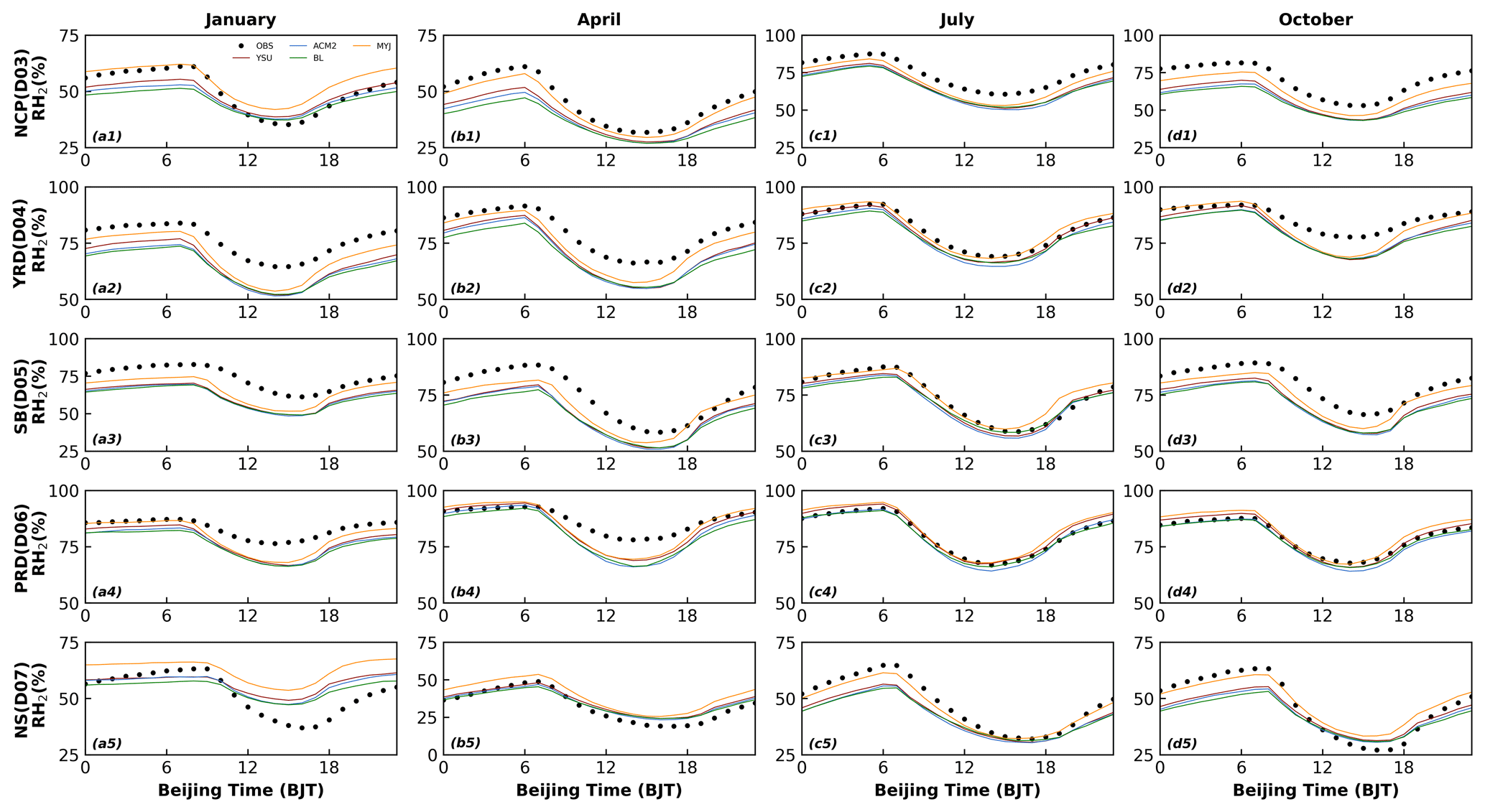
The results for 2 m relative humidity (RH₂) and T₂ correspond to each other, and the overestimation of T₂ corresponds to the underestimation of RH₂. The simulation of RH₂ still shows the best results in July, with the highest simulated values for the MYJ scheme and the lowest for the BL scheme. Except for the NS region, the simulated RH₂ of the other four regions is almost underestimated. This uniform trend in relative humidity may be due to errors in the initial field, which will be discussed in Part 2. Not everything will be repeated here (Figs. 2, 7).

Figure 7 Similar to Fig. 2 but for 2 m relative humidity.

3.1.2 The 10 m wind speed and direction

Although the model simulates the diurnal cycle of wind speed, the wind speed shows different degrees of overestimation, and the mean bias is in the range of 0.86–2.74 m s⁻¹ (Fig. 8, Table 2). This is also the conclusion reached in many previous studies and it is more widely accepted by the public (Cohen et al., 2015; Jia and Zhang, 2020, 2021; Jiménez and Dudhia, 2012). Except for the NCP region where the MYJ scheme has the largest mean bias (MB) value during the day (YSU: MB = 1.6 m s⁻¹; ACM2: MB = 1.8 m s⁻¹; BL: MB = 1.7 m s⁻¹; MYJ: MB = 2.1 m s⁻¹), while the BL scheme has the largest MB value at night regardless of the region (YSU: MB = 1.3 m s⁻¹; ACM2: MB = 1.8 m s⁻¹; BL: MB = 2.2 m s⁻¹; MYJ: MB = 1.7 m s⁻¹) (Fig. 8, Table 2).

Figure 8 Similar to Fig. 2 but for 10 m wind speed.

Table 2 Mean bias of 2 m temperature, 2 m relative humidity, and 10 m wind speed during daytime and nighttime by four PBL schemes in five regions and four seasons.

Similar to T₂, 10 m wind speed (i.e., WS₁₀) is also a diagnostic variable of the near-surface wind speed. For the YSU, ACM2, and BL schemes, in the revised MM5 surface layer scheme, WS₁₀ is calculated based on the Monin-Obukhov (M–O) similarity theory (Monin and Obukhov, 1954). The dimensionless profile function of momentum is denoted as follows:

$$\begin{array}{}\text{(23)}& {\mathit{\varphi }}_{\mathrm{m}}\left({\displaystyle \frac{z}{L}}\right)={\displaystyle \frac{\mathit{\kappa }z}{u_{\ast }}}{\displaystyle \frac{\partial u}{\partial z}}\end{array}$$

where κ is the von Kármán constant, u_∗ is the friction velocity, z is the height, and L is the Obukhov length, integrating the Eq. (23) with respect to height z:

$$\begin{array}{}\text{(24)}& \mathrm{d}u={\displaystyle \frac{u_{\ast }}{\mathit{\kappa }}}\left[{\displaystyle \frac{\mathrm{d}z}{z}}-{\displaystyle \frac{\mathrm{1}-{\mathit{\varphi }}_{\mathrm{m}}\left(\frac{z}{L}\right)}{\frac{z}{L}}}d\left({\displaystyle \frac{z}{L}}\right)\right],\end{array}$$

and after integrating Eq. (24):

$$\begin{array}{}\text{(25)}& \underset{\mathrm{0}}{\overset{u}{\int }}\mathrm{d}u={\displaystyle \frac{u_{\ast }}{\mathit{\kappa }}}\left\{\underset{z_{\mathrm{0}}}{\overset{z}{\int }}{\displaystyle \frac{\mathrm{d}z}{z}}-\underset{\frac{z_{\mathrm{0}}}{L}}{\overset{\frac{z}{L}}{\int }}\left[\mathrm{1}-{\mathit{\varphi }}_{\mathrm{m}}\left({\displaystyle \frac{z}{L}}\right)\right]d\ln \left({\displaystyle \frac{z}{L}}\right)\right\},\end{array}$$

here, let ${\mathit{\psi }}_{\mathrm{m}}\left(\frac{z}{L}\right)={\int }_{\mathrm{0}}^{\frac{z}{L}}\left[\mathrm{1}-{\mathit{\varphi }}_{\mathrm{m}}\left(\frac{z}{L}\right)\right]\mathrm{d}\ln \left(\frac{z}{L}\right)$, where ${\mathit{\psi }}_{\mathrm{m}}\left(\frac{z}{L}\right)$ is the integrated similarity function for momentum.

Therefore, Eq. (25) can be given as $u=\frac{u_{\ast }}{\mathit{\kappa }}\left[\ln \left(\frac{z}{z_{\mathrm{0}}}\right)-{\mathit{\psi }}_{\mathrm{m}}\left(\frac{z}{L}\right)+{\mathit{\psi }}_{\mathrm{m}}\left(\frac{z_{\mathrm{0}}}{L}\right)\right]$, where z₀ is the roughness length.

Based on the bulk transfer method, the momentum flux can be represented as $\mathit{\tau }=\mathit{\rho }{u}_{\ast }^{\mathrm{2}}=\mathit{\rho }{C}_{\mathrm{m}}{u}^{\mathrm{2}}$, where τ is the momentum flux and C_m is the bulk transfer coefficient for momentum:

$$\begin{array}{}\text{(26)}& C_{\mathrm{m}}={\displaystyle \frac{u_{\ast }^{\mathrm{2}}}{u^{\mathrm{2}}}}={\displaystyle \frac{{\mathit{\kappa }}^{\mathrm{2}}}{{\left[\ln \left(\frac{z}{z_{\mathrm{0}}}\right)-{\mathit{\psi }}_{\mathrm{m}}\left(\frac{z}{L}\right)+{\mathit{\psi }}_{\mathrm{m}}\left(\frac{z_{\mathrm{0}}}{L}\right)\right]}^{\mathrm{2}}}},\end{array}$$

Thus, the wind speed at 10 m divided by the wind speed at a certain height can be written as follows:

$$\begin{array}{}\text{(27)}& \begin{array}{rl}{u}_{\mathrm{10}}& ={\displaystyle \frac{u_{\ast }}{\mathit{\kappa }}}\left[\ln \left({\displaystyle \frac{z}{z_{\mathrm{0}}}}\right)-{\mathit{\psi }}_{\mathrm{m}}\left({\displaystyle \frac{z}{L}}\right)+{\mathit{\psi }}_{\mathrm{m}}\left({\displaystyle \frac{z_{\mathrm{0}}}{L}}\right)\right]\\ & \cdot {\displaystyle \frac{\left[\ln \left(\frac{\mathrm{10}}{z_{\mathrm{0}}}\right)-{\mathit{\psi }}_{\mathrm{m}}\left(\frac{\mathrm{10}}{L}\right)+{\mathit{\psi }}_{\mathrm{m}}\left(\frac{z_{\mathrm{0}}}{L}\right)\right]}{\left[\ln \left(\frac{z}{z_{\mathrm{0}}}\right)-{\mathit{\psi }}_{\mathrm{m}}\left(\frac{z}{L}\right)+{\mathit{\psi }}_{\mathrm{m}}\left(\frac{z_{\mathrm{0}}}{L}\right)\right]}}=\\ & {\displaystyle \frac{u_{\ast }}{\mathit{\kappa }}}\left[\ln \left({\displaystyle \frac{z}{z_{\mathrm{0}}}}\right)-{\mathit{\psi }}_{\mathrm{m}}\left({\displaystyle \frac{z}{L}}\right)+{\mathit{\psi }}_{\mathrm{m}}\left({\displaystyle \frac{z_{\mathrm{0}}}{L}}\right)\right]\cdot {\left({\displaystyle \frac{C_{\mathrm{m}}}{C_{\mathrm{m}\mathrm{10}}}}\right)}^{\mathrm{1}/\mathrm{2}}\end{array},\end{array}$$

where C_m10 is the transfer coefficient for momentum at 10 m height:

$$\begin{array}{}\text{(28)}& C_{\mathrm{m}\mathrm{10}}={\displaystyle \frac{{\mathit{\kappa }}^{\mathrm{2}}}{{\left[\ln \left(\frac{\mathrm{10}}{z_{\mathrm{0}}}\right)-{\mathit{\psi }}_{\mathrm{m}}\left(\frac{\mathrm{10}}{L}\right)+{\mathit{\psi }}_{\mathrm{m}}\left(\frac{z_{\mathrm{0}}}{L}\right)\right]}^{\mathrm{2}}}}.\end{array}$$

Comparing the C_m of the three schemes (i.e., YSU, ACM2, and BL schemes) at night, C_m is the largest for the BL scheme, the second largest for the ACM2 scheme, and the smallest for the YSU scheme (Fig. 9). Correspondingly, the BL scheme simulates the largest WS₁₀, ACM2 the second largest, and the YSU the smallest (Fig. 8). The larger C_m corresponds to the stronger mixing, which transports more momentum from the upper to the lower layers, making WS₁₀ increase. Therefore, the bulk transfer coefficient C_mcontrols the variation in WS₁₀ at night. During the daytime, the C_m of the BL scheme is smaller than that of the other two schemes and the corresponding WS₁₀ decrease (Figs. 8, 9). However, the difference among the three schemes is smaller in daytime than that in nighttime. The reason why the results of C_m and WS₁₀ differ with the same calculation method is because of the vertical variation in heat and momentum within the boundary layer involved in the calculation. This will correlate to the vertical diffusion coefficients within the boundary layer that will be discussed further in a later section.

Figure 9 Similar to Fig. 2 but for momentum transfer coefficient (C_m).

For the near-surface scheme of the MYJ scheme, WS₁₀ is calculated according to the near surface flux profile relationship proposed by Liu et al. (1979):

$$\begin{array}{}\text{(29)}& u_{\mathrm{0}}-u_{\mathrm{s}}=D_{\mathrm{1}}\left[\mathrm{1}-\exp \left(-{\displaystyle \frac{z_u{u}_{\ast }}{D_{\mathrm{1}}\mathit{\nu }}}\right)\right]\left({\displaystyle \frac{F_u}{u_{\ast }}}\right),\end{array}$$

where 0 represents the value at height z above the surface where the molecular diffusivity still plays a dominant role, s denotes the surface value, D₁ denotes a near-surface parameter, u_∗ is the friction velocity, ν is the molecular diffusivity for momentum ($=\mathrm{1}\times {\mathrm{10}}^{-\mathrm{5}}$), and F_u is the momentum flux. Since $\mathrm{1}-\exp \left(-\frac{z_u{u}_{\ast }}{D_{\mathrm{1}}\mathit{\nu }}\right)\approx \frac{z_u{u}_{\ast }}{D_{\mathrm{1}}\mathit{\nu }}$, $u_{\mathrm{0}}-u_{\mathrm{s}}=\left(\frac{z_u}{\mathit{\nu }}\right)F_u$.

The momentum flux in the surface layer above the viscous sublayer is represented by $F_u=\left(\frac{C_{\mathrm{m}}}{\mathrm{\Delta }{z}_{\mathrm{e}}}\right)\left(u_{\mathrm{low}}-u_{\mathrm{0}}\right)$; here, the subscript low denotes the variables at the lowest model level and Δz_e is the equivalent height of the lowest model level that considers the presence of the “dynamical turbulence layer” at the bottom of the surface layer (Janjić, 1990). C_m is the bulk transfer coefficient, defined as follows:

$$\begin{array}{}\text{(30)}& C_{\mathrm{m}}={\displaystyle \frac{\mathit{\kappa }{u}_{\ast }}{\ln \left(\frac{z_{\mathrm{0}}+z}{z_{\mathrm{0}}}\right)+{\mathit{\psi }}_{\mathrm{m}}\left(\frac{z_{\mathrm{0}}+z}{L}\right)-{\mathit{\psi }}_{\mathrm{m}}\left(\frac{z_{\mathrm{0}}}{L}\right)}}.\end{array}$$

In Eq. (29), z_u is still an unknown, such that $\frac{z_u{u}_{\ast }}{D_{\mathrm{1}}\mathit{\nu }}=\mathit{\xi }$, where ξ is a smaller constant (equal to 0.35 in the model). Here, the near-surface parameter D₁ is further defined as $D_{\mathrm{1}}=C\cdot {\left(\frac{z_{\mathrm{0}}{u}_{\ast }}{\mathit{\nu }}\right)}^{\mathrm{1}/\mathrm{4}}$, where C is a constant (=30), the roughness length z₀ as a function of u_∗ ($z_{\mathrm{0}}=\frac{\mathrm{0.11}\mathit{\nu }}{u_{\ast }}+\frac{\mathrm{0.018}{u}_{\ast }^{\mathrm{2}}}{g}$), substituting D₁ and z_u to Eq. (29):

$$\begin{array}{}\text{(31)}& u_{\mathrm{0}}={\displaystyle \frac{\frac{\mathit{\xi }}{u_{\ast }}\left[C\cdot {\left(\frac{z_{\mathrm{0}}{u}_{\ast }}{\mathit{\nu }}\right)}^{\mathrm{1}/\mathrm{4}}\right]\left(\frac{C_{\mathrm{m}}}{\mathrm{\Delta }{z}_{\mathrm{e}}}\right)u_{\mathrm{low}}+u_{\mathrm{s}}}{\mathrm{1}+\frac{\mathit{\xi }}{u_{\ast }}\left[C\cdot {\left(\frac{z_{\mathrm{0}}{u}_{\ast }}{\mathit{\nu }}\right)}^{\mathrm{1}/\mathrm{4}}\right]\left(\frac{C_{\mathrm{m}}}{\mathrm{\Delta }{z}_{\mathrm{e}}}\right)}}.\end{array}$$

The wind speed at a height of 10 m can be expressed as follows:

$$\begin{array}{}\text{(32)}& u_{\mathrm{10}}={\displaystyle \frac{F_u\mathrm{\Delta }{z}_{\mathrm{e}}}{C_{\mathrm{m}\mathrm{10}}}}+u_{\mathrm{0}}={\displaystyle \frac{C_{\mathrm{m}}\left(u_{\mathrm{low}}-u_{\mathrm{0}}\right)}{C_{\mathrm{m}\mathrm{10}}}}+u_{\mathrm{0}},\end{array}$$

where C_m10 is the transfer coefficient for momentum at 10 m height:

$$\begin{array}{}\text{(33)}& C_{\mathrm{m}\mathrm{10}}={\displaystyle \frac{\mathit{\kappa }{u}_{\ast }}{\ln \left(\frac{z_{\mathrm{0}}+\mathrm{10}}{z_{\mathrm{0}}}\right)+{\mathit{\psi }}_{\mathrm{m}}\left(\frac{z_{\mathrm{0}}+\mathrm{10}}{L}\right)-{\mathit{\psi }}_{\mathrm{m}}\left(\frac{z_{\mathrm{0}}}{L}\right)}}.\end{array}$$

Therefore, the C_m of the MYJ scheme is significantly different from the other three schemes. Except for the NCP region, although the C_m of the MYJ scheme is larger than the other three schemes at all times of the day, the WS₁₀ presents the maximum only during the daytime. This suggests that at night, the wind speed simulated by the MYJ scheme also be influenced by other factors. For example, the calculation method of the integrated similarity functions (ψ_m) in the MYJ scheme is different from the other three schemes. In the other three schemes, the ψ_m is calculated according to four stability regimes defined in terms of the bulk Richardson number (Zhang and Anthes, 1982). In the MYJ scheme, the ψ_m is calculated based on two stability regimes by the $z/L$ (Paulson, 1970).

Figure 10 Similar to Fig. 5 but for 10 m wind speed.

The reasons for the differences in WS₁₀ simulation are further analyzed in terms of regional distribution. During the daytime, wind speed is significantly overestimated at most sites throughout the NCP region, which are centered in the plains and valleys but is less overestimated and even underestimated at some sites on the mountain tops (Figs. 10, S13–S15a1–e1). Wind speed is overestimated at almost all stations throughout the YRD and PRD regions (Figs. 10, S13–S15a2–e2, a4–e4). The WS₁₀ in the basin is importantly overestimated in the SB region and less overestimated at hilltop stations on the eastern side of the basin, with higher wind speed being more pronounced in January (Figs. 10, S13–S15a3–e3). In the NS region, wind speed is overestimated to a lesser extent than in other regions, but for regions with lower wind speed, the relative bias (RB) is larger, especially in July (January: RB = 29.3 %–49.1 %; April: RB = 32.0 %–55.6 %; July: RB = 44.2 %–78.7 %; October: RB = 42.7 %–65.7 %). Comparing the simulation results of the four schemes, the MYJ scheme simulates the most significantly overestimated wind speed and the least overestimated for the YSU scheme (Figs. 10, S13–S15). In comparison with the 4 months, it is found that the RB of the simulation is the largest for the month with slower wind speed (i.e., July).

At night, the wind speed is overestimated at almost all stations in the whole region of NCP, and the overestimation is greater at the hilltop stations than during the day (Figs. 11, S16–S18). The other four regions are more similar to the daytime (Figs. 11, S16–S18). However, by comparing the four schemes, we find that the BL scheme has the most obvious overestimation, different from the daytime, while the YSU scheme still has the lowest overestimation, the same as the daytime. In general, wind speed is smaller at night, and the four schemes overestimate wind speed much more than during the day. Averaging the RB of wind speed over the five regions and 4 months, the daytime (nighttime) values for the YSU, ACM2, BL, and MYJ schemes are 77.7 % (92.4 %), 85.6 % (123.6 %), 80.2 % (146.0 %), and 100.8 % (117.4 %), respectively. This simulated misestimation of low winds at night may mainly originate from the inapplicability of the M-O similarity theory. The strong stable boundary layer usually occurs on nights with low winds (Monahan and Abraham, 2019; Vignon et al., 2017). In this strong stable boundary layer, turbulence occurs weakly and intermittently, the turbulence intensity is disproportionate to the mean gradient, and the M-O similarity theory is no longer applicable (Acevedo et al., 2015; Sun et al., 2012). Ultimately, these inapplicable functions affect the calculation of the bulk transfer coefficient and can further lead to large deviations in the simulation of wind speed.

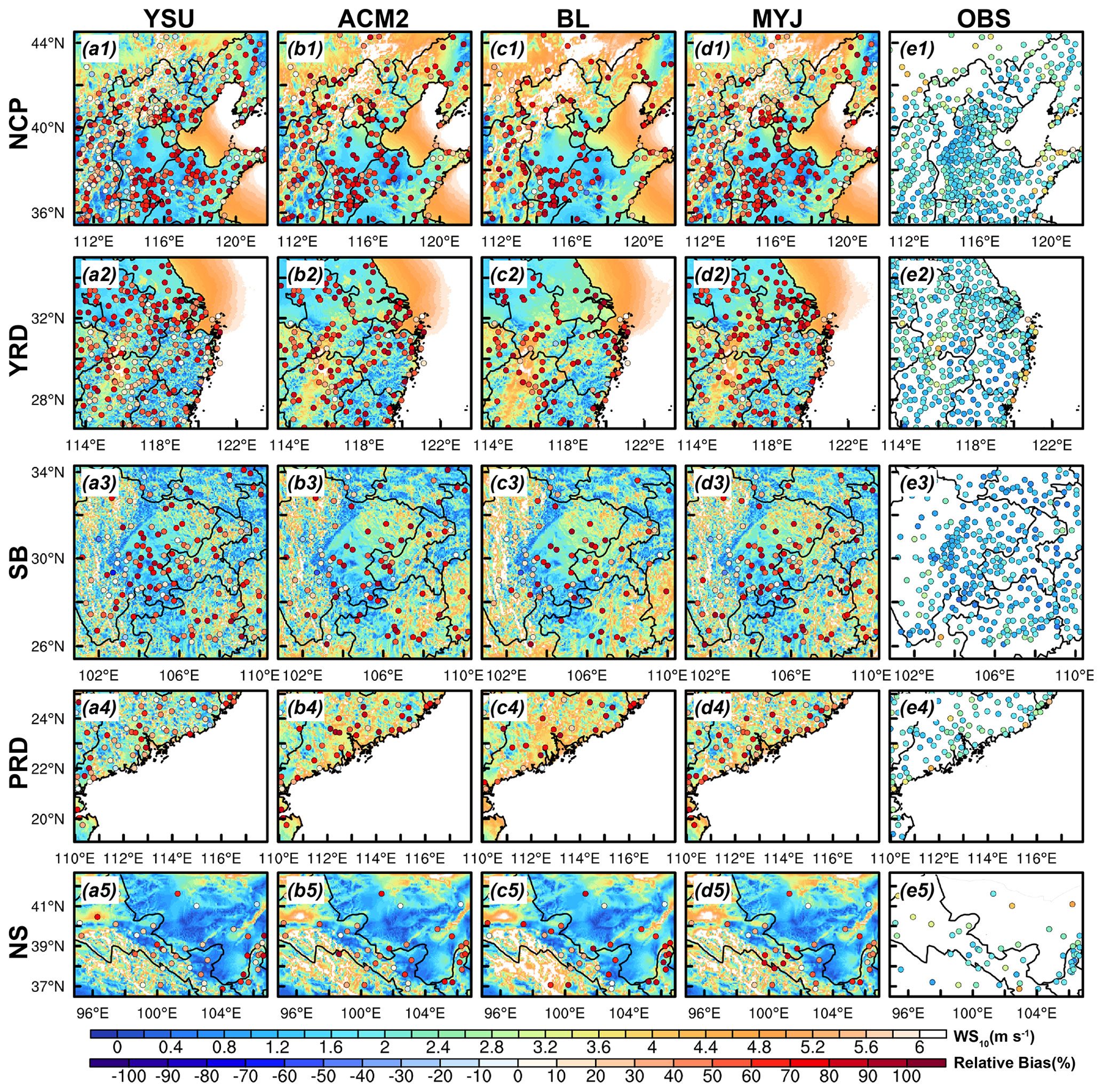
Figure 11 Similar to Fig. 6 but for 10 m wind speed.

We further re-analyze the effect of topography on wind speed. The wind speed is overestimated for plains and valleys and better reproduced or underestimated for mountain tops, mainly because of the smoother topography in the model. This is rather because coastal stations in the plains, many of which also have high wind speeds, are not well reproduced and still show significant overestimation (Fig. 10) compared to the high wind speeds at the top of the mountains, which are better simulated. It is assumed that the wind speed should be small in plain areas with complex underlying surfaces, but it increases after the model has smoothed the terrain. The wind speed increases gradually with height, and when the terrain at the top of the mountain is smoothed, the originally larger wind speed decreases, and the wind speed will be closer to the observed value.

Figure 12 Similar to Fig. 2 but for 10 m wind direction.

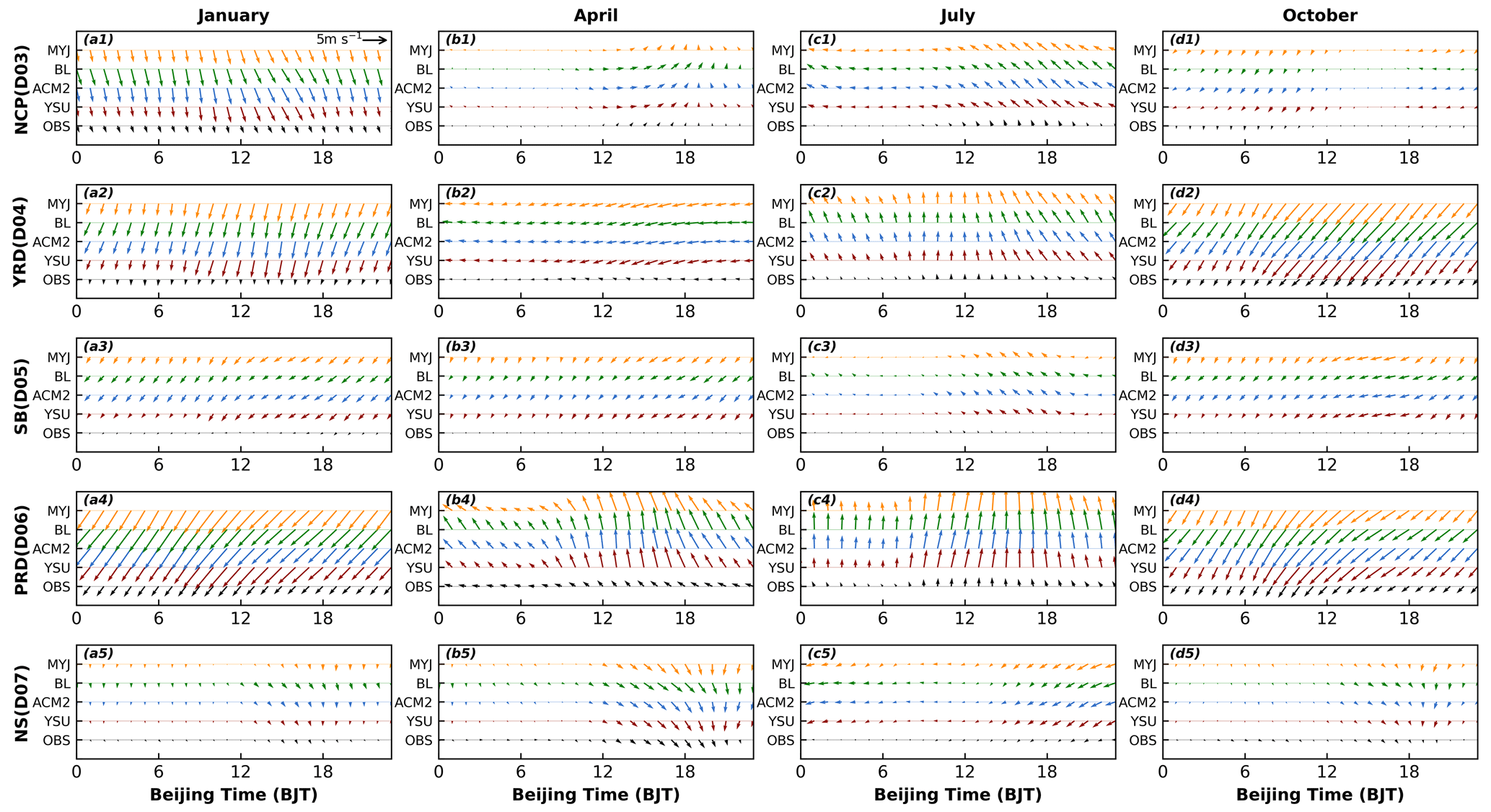
The model can basically simulate the changes in wind direction in the five regions, capturing the overall wind direction well in each region (Fig. 12). In the NCP region, the simulation of wind direction is poor in January compared to the other 3 months, with a high frequency of northwesterly and northerly winds, overestimated by about 6.6 % (Fig. 13a1–d1). In addition, coupled with larger wind speed, it causes the effect of advective transport to be amplified, thus affecting the variation in pollutant concentrations (Jia and Zhang, 2021). The frequency of simulated northeasterly winds in the YRD region is higher than that observed in January (∼ 6.9 %), April (∼ 6.9 %), and October (∼ 11.2 %), while the frequency of southerly winds is higher in July (∼ 10.0 %) (Fig. 13a2–d2). The wind direction of SB region is poorly simulated since the topography is too complicated in the SB region, with a basin in the middle and high topographic mountains all around (Fig. 13a3–d3). The low wind state in the middle of the basin is difficult to be captured. The percentage of northeasterly winds simulated by the model in January, April, July, and October are 22.9 %–25.6 %, 19.2 %–20.6 %, 14.9 %–16.4 %, 22.4 %–24.2 %, respectively, and the percentage of observations are 15.1 %, 12.0 %, 10.9 %, 16.1 %, respectively. Similarly, the percentage of westerly winds simulated by the model in January, April, July, and October are 4.7 %–5.1 %, 4.7 %–5.7 %, 4.8 %–5.5 %, 3.8 %–5.1 %, respectively, and the percentages of observations are 9.9 %, 12.4 %, 12.4 %, 12.3 %, respectively. The model simulates a large proportion of northeasterly winds and a smaller proportion of westerly winds (Fig. 13a3–d3). In the PRD region, the frequency of northeasterly wind occurrences in January and October is significantly overestimated by about 8.8 % and 9.5 %, while the frequency of southerly winds is overestimated in April and July by about 14.5 % and 17.3 %, and the frequency of southeasterly winds is underestimated (Fig. 13a4–d4). The wind direction is better simulated in the NS region, not significantly influenced by the complex terrain (Fig. 13a5–d5).

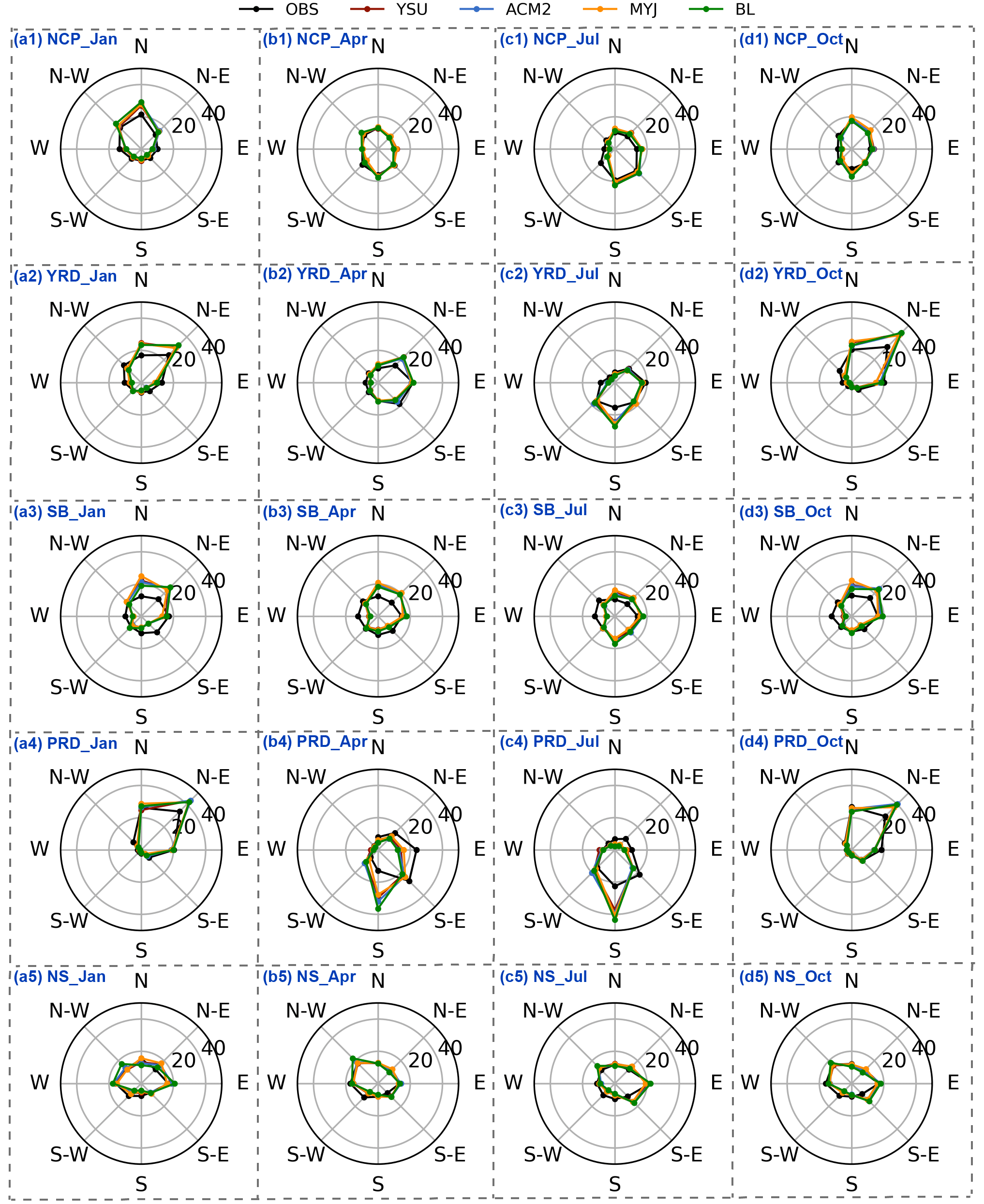
Figure 13 Wind rose plots in five regions for four seasons for the (a1–d1) NCP region, (a2–d2) YRD region, (a3–d3) SB region, (a4–d4) PRD region and (a5–d5) NS region, respectively.

3.2 Vertical structures

To better understand the performance of model in simulating PBL structure under different underlying surface, four representative stations have been selected in each region, with stations in plain areas, stations in mountains areas with high elevation, and stations near the sea.

3.2.1 Temperature

Accurate simulation of the vertical structure of the PBL is very important for the evolution of pollution, precipitation, and typhoons. In the vertical direction, four typical sounding stations are selected for each region at 08:00 BJT to better reflect the simulation of the vertical structure of the PBL under different underlying surface conditions. Overall, the model captures the vertical structures of the temperature. From the simulation results in January, the best reproduction of the temperature simulation is found in the YRD region, in which the temperature is closer to the observed values (Fig. 14a2–d2). In addition to the NCP, SB, and NS regions, a temperature inversion layer appears in the lower layers at 08:00 BJT, and the NS region has the most significant temperature inversion (Fig. 14a1–d1, a3–d3, a5–d5). The model does not simulate the temperature variation in the inversion layer well and shows significant differences from the observations. When there is a difference in topography between the observed and simulated stations, the bias in the temperature is more pronounced. These stations usually exist in complex topographic conditions, such as Zhangjiakou and Zhangqiu stations in the NCP region, Shapingba in the SB region, and Mazongshan and Jiuquan in the NS region (Fig. 14b1, d1, c3, a5, b5). The topographic discrepancy caused by the lack of high resolution may, on the one hand, account for it, resulting in more complex topography in the grid points closest to the observation stations. On the other hand, there is also an urgent need for finer underlying surface data to respond more closely to the observed real topography. The effect of resolution and underlying surface will be discussed in detail in the Part 2. Although the elevation of the Hongyuan station in the SB region is higher, the differences in topographic height obtained from observations and simulations are close to each other (Fig. 14a3).

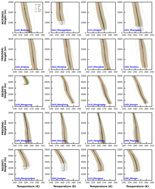
Figure 14 Average vertical profiles of observed and simulated temperature at 08:00 and 20:00 BJT at four sounding stations for each region in January (winter). The unobtrusive gray lines indicate the simulated lines for all time periods, and the lines with shading indicate the average values and shaded areas show the uncertainty range (the mean ±1 standard deviation).

There is an underestimation of temperature at stations with higher topography and overestimation for lower topography, which is more consistent with the conclusions drawn from 2 m temperature (Figs. 5, 14). However, the underestimation of temperature is not present throughout the vertical, but it is more pronounced in the lower layers, which are more influenced by the underlying surface. From the differences in the four schemes, the MYJ scheme simulates the lowest temperature and largest temperature gradient. Since the MYJ scheme simulates a weak turbulent diffusion of heat, a well vertical exchange process cannot occur, bringing into a large temperature gradient (Fig. S19). The differences in the four schemes gradually decrease with the increase in height. The BL scheme, which is also a local closure scheme, has a smaller vertical gradient in temperature, mainly because this scheme adds a counter-gradient correction term to the heat flux, which is mainly applicable to the convective PBL (Bougeault and Lacarrere, 1989). The presence of this term leads to an increase in turbulent diffusion and a decrease in temperature gradient. However, it is worth noting that there are still slightly stable stratifications at 08:00 BJT, and this term generates upward heat flux and reduces the temperature gradient, which is closer to the results of the nonlocal closure schemes (YSU and ACM2 schemes). The simulation results for the other 3 months are not as good as January, but the simulation characteristics are similar to January (figures not shown). The results at 20:00 BJT are similar to those at 08:00 BJT , and thus they will not be repeated here (figures not shown).

3.2.2 Wind speed and direction

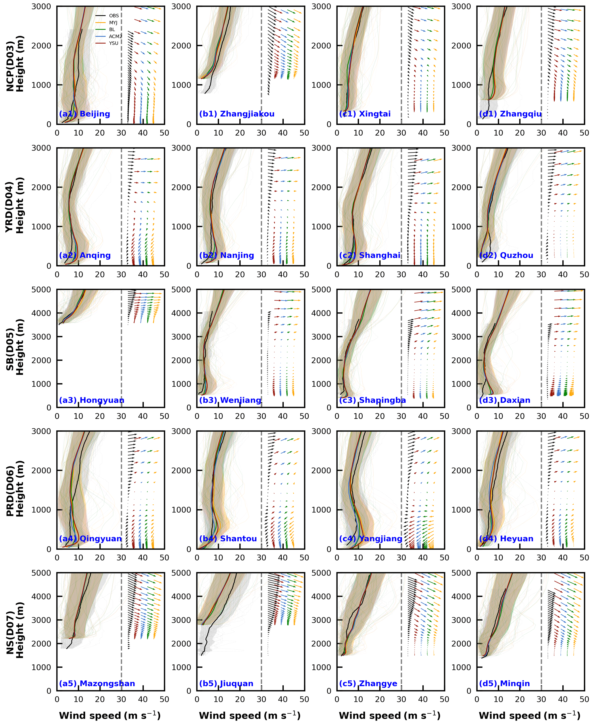
The simulation of wind speed vertical structure is much worse in comparison to temperature (Figs. 14, 15). The simulated results of wind speed in the vertical direction and 10 m wind speed are still quite different. In the 4 months, the wind speed is almost overestimated at the lower-altitude stations below 1000 m in all regions except the NS region, and wind speed is less overestimated in July than in the other 3 months (Figs. 15, S20–S22a1–d4). However, for the NS region, the wind speed is almost better simulated or underestimated and is significantly different from the other four regions (Figs. 15, S20–S22a5–d6). We can compare the Zhangjiakou station in the NCP region with the Hongyuan station in the SB region and find that the wind speeds at these stations are almost not overestimated (Fig. 15b1, a3). The effect of the model on terrain smoothing contributes to this. Because the wind speed itself increases with the increase in height, it decreases when the model smooths over the terrain.

Unlike the 10 m wind speed, the simulation results of the 10 m wind speed have the smallest bias for the YSU scheme, which is closer to the observed value (Table 2, Figs. 8, 10–11). Of course, this phenomenon can also be found from the evolution of the wind speed in the vertical direction (Figs. 15, S20–S22). However, as the height increases, the bias of the YSU scheme gradually increases and is greater than the other three schemes (Figs. 15, S20–S22). Such a large vertical gradient of wind speed in the YSU scheme indicates a weak mixing in this scheme. From the turbulent diffusion coefficients of the momentum at 08:00 BJT in January, it is true that the YSU scheme simulates the smallest turbulent diffusion coefficient below 1000 m (Fig. S23). While the BL scheme simulates a smallest vertical gradient of wind speed, which corresponds to the largest turbulent diffusion coefficient of momentum (Fig. S23). The time variation characteristics of the turbulent diffusion coefficient will be deliberated and analyzed in detail later.

The simulation results of wind direction notes that the model can capture the characteristics of wind direction well, and it also simulates them well for the stations with more complicated topography and higher altitude (Figs. 15, S20–S22).

Figure 15 Similar to Fig. 14 but for the vertical profile of wind speed and direction.

3.3 PBLH

Since the observations are only available at 08:00 and 20:00 BJT, the comparisons of the PBLH are all the result of these two moments. Based on the observed data, comparing the PBLH calculated by the two methods, it is found that the results are mixed for two methods (Fig. 16). The results for January (IOA = 0.70–0.90) are better than the other 3 months (IOA = 0.44–0.88 in April, IOA = 0.51–0.86 in July, and IOA = 0.60–0.77 in October), and the results in the NCP region are better than the other four regions (Fig. 16). The PBLH in the NS region is more scattered, unlike the other regions where most of the PBLH is concentrated below 500 m, especially in April and July (Fig. 16b5–c5). On the whole, the difference in PBLH calculated by the two methods is more obvious in the NS region with its more complex topography, which is especially noted when calculating in this type of underlying surface region.

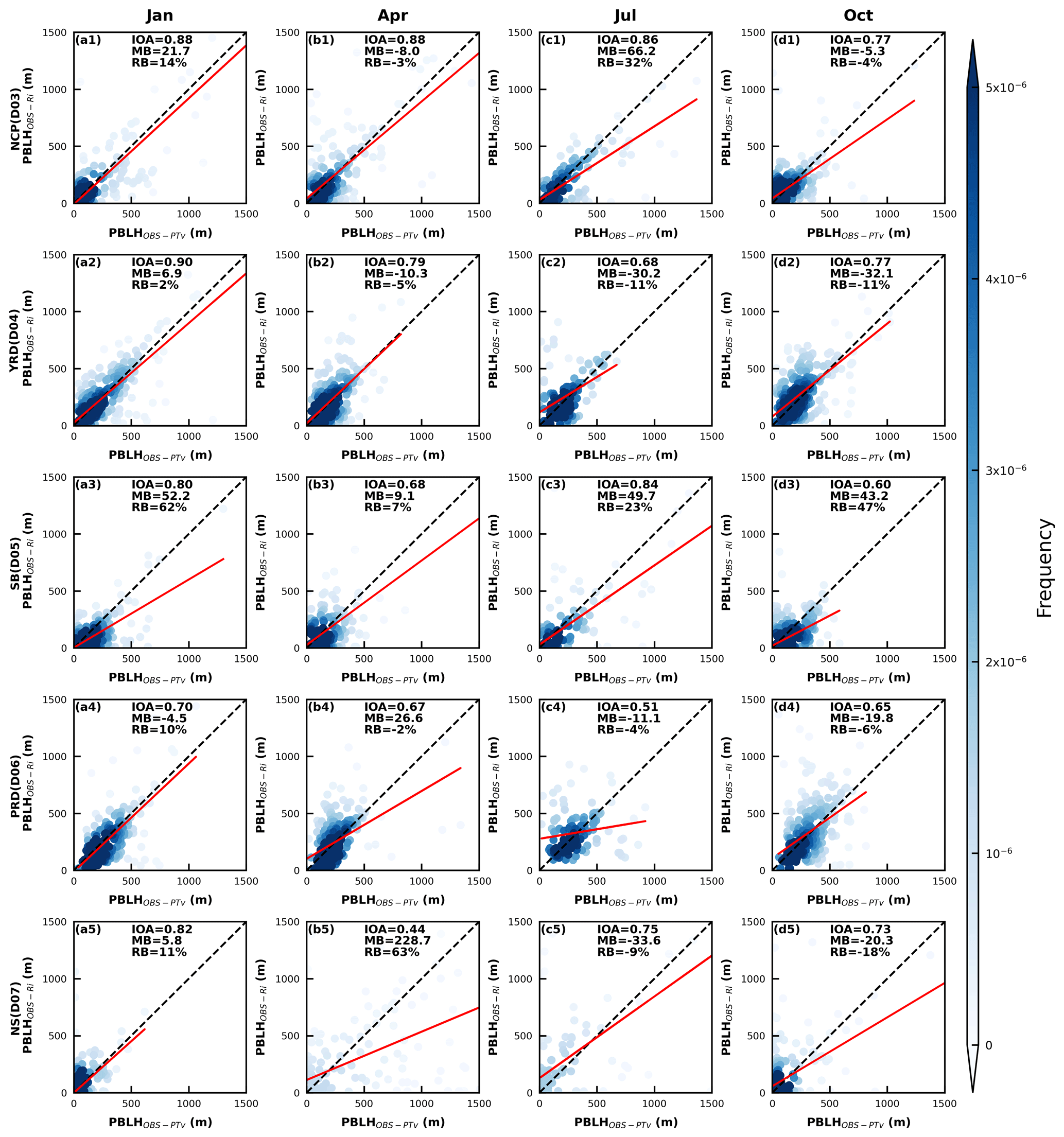
Figure 16 Density scatterplots of the PBLH at 08:00 and 20:00 BJT by the two methods in five regions for four seasons. The horizontal and vertical coordinates represent the PBLH calculated based on the observed data using the virtual temperature method and the Richardson number method, respectively, and IOA, MB, and RB represent the index of agreement, mean bias, and relative bias, respectively.

Further, the mechanism of understanding the PBLH differs based on different stations from different regions. The PBLH for the YSU and ACM2 schemes is calculated by the Richardson number method, and the PBLH for the BL scheme is obtained by the virtual potential temperature method (see Sect. 2 for details). The same two methods are also used to calculate the PBLH with sounding data for comparison (Eqs. 15 and 16). First, we compare the PBLH calculated based on the observed data using Richardson number (Ri) with the PBLH simulated by YSU and ACM2 schemes. The Ri is determined by both the buoyancy term and the shear term (Eq. 15). The difference between simulated and observed temperature gradient is smaller than the wind speed gradient within the PBL (Figs. 14–15). Therefore, the difference in Ri mainly comes from the variation in the shear term. The wind speed gradients simulated in both schemes are greater than the observed values (Fig. 15), except for individual stations, which would result in small values of Ri. Thus, the height of Ri up to 0.25 would be high, and the PBLH would also be high. Consequently, the PBLH simulated by the YSU and ACM2 schemes are higher than the observed values at most stations. For example, in the case of the Quzhou station in the YRD region, the simulated wind speed gradient at this station is much smaller than the observed value in January; thus, the simulated PBLH is correspondingly smaller than PBLH calculated from observations (Figs. 15, S24d2). Comparing the results of the other 3 months, we can also find similar conclusions (figures not shown). The wind speed gradient simulated by the YSU scheme is larger than that of the ACM2 scheme, and therefore the PBLH is larger than that of the ACM2 scheme, except for the Shanghai station in the YRD region and Shantou and Yangjiang stations in the PRD region (Fig. S24). For the ocean, the PBLH simulated by the ACM2 scheme is higher than that of the YSU scheme, while for most areas adjacent to the ocean, the PBLH simulated by the ACM2 scheme is on the high side in the YRD and PRD regions (Fig. S25). The simulated PBLH of the BL scheme is in better agreement with the PBLH calculated by the virtual potential temperature method, which is substantially better than the other three schemes. The PBLH simulated by the MYJ scheme is mixed (Fig. 17).

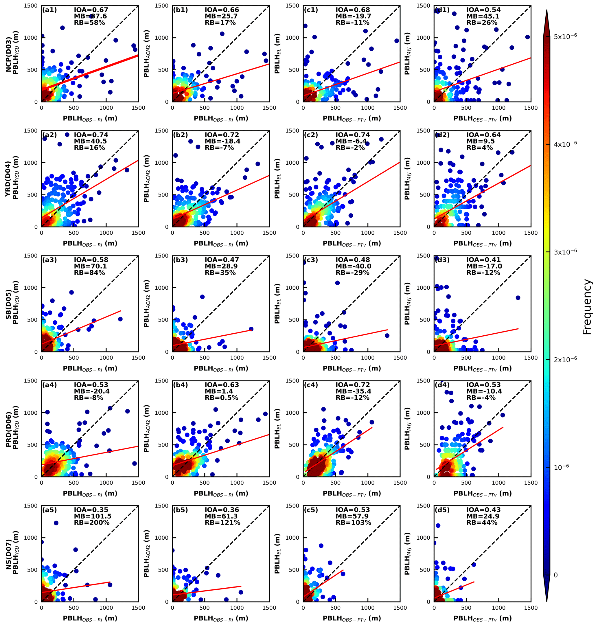
Figure 17 Density scatterplots of observed and simulated PBLH at 08:00 and 20:00 BJT by four PBL schemes in five regions in January (winter). The horizontal and vertical subscripts YSU, ACM2, BL, and MYJ indicate the four schemes, while OBS-Ri and OBS-PTv indicate the Richardson number method and virtual potential temperature method, respectively.

From the differences in regional distributions, the region with the best PBLH simulation results is the YRD region in January, (IOA = 0.64–0.74; MB = −6.4–40.5 m; RB = −2 %–16 %), followed by the PRD region (IOA = 0.53–0.72; MB = −35.4–1.4 m; RB = −12 %–0.5 %), and the worst simulation results are for the PBLH in the NS region (IOA = 0.35–0.53; MB = 24.9–101.5 m; RB = 44 %–200 %) (Fig. 17). Also, the PBLH simulation in the SB region is poorer and slightly better than that in the NS region, noting that there is still much potential for the model to improve the reproduction of the PBLH in complex terrain. From the simulation results of the four schemes, the PBLH simulated by the BL scheme is the closest to the observed value, followed by the YSU and ACM2 schemes, and the PBLH simulated by the MYJ scheme is the worst. However, it is worth noting here that the method for calculating the PBLH in the MYJ scheme is the TKE, and there is still some uncertainty in the comparison using the virtual potential temperature method. The simulation results of temperature are better than other meteorological parameters; therefore, the PBLH calculated in the model using the virtual potential temperature method is more consistent with the observed results. While as the YSU and ACM2 schemes using the Richardson number method will involve the wind speed gradient, and the vertical gradient of wind speed is poorly simulated below 1000 m. That is why it will affect the judgment of the PBLH. If the simulation results of vertical gradient of wind speed can be improved subsequently, then the simulation results of PBLH of these two schemes will be improved to some extent. There are not enough observations to calculate the PBLH using TKE, so there will be some differences with the PBLH simulated by the MYJ scheme. The mean bias of the simulation increased in April and July when the PBLH is higher compared to January, with a mean bias of −29.6–361.8 m (6.5–603.9 m), −12.6–410.6 m (41.6–603.2 m), −34.1–301.1 m (3.2–683.9 m), and −14.5–96.3 m (−11.3–523.6 m) for the YSU, ACM2, BL and MYJ schemes in April (July), respectively. Similar to January, the best simulation results have been obtained for the YRD (MB = 7.8–72.4 m in April, MB = 28.5–66.5 m in July) and PRD (MB = −34.1–12.6 m in April, MB = −11.3–54.8 m in July) regions, and the worst are found for the NS region (MB = 61.8–410.6 m in April, MB = 523.6–683.9 m in July). The results for October are more similar to those for January, with lower PBLH and better simulations than those for April and July (figures not shown).

3.4 Turbulent diffusion coefficient

Since the model itself does not directly output turbulent diffusion coefficients for all schemes, there is relatively little direct comparison and analysis of this parameter. As seen in Sect. 3.2.2 above, the TDC plays a crucial role in the momentum vertical transport within the PBL and also has an impact on the diffusion of other parameters, such as heat, water vapor, and pollutants (Ding et al., 2021; Stull, 1988). The accurate portrayal of the TDC directly affects the evolution of the PBL structures. Based on the contents of Sect. 2.3, the momentum TDC is not equal to the heat TDC under unstable and neutral conditions for the YSU scheme, and the momentum TDC is equal to the heat TDC under stable conditions. The ACM2 scheme uses the MOST method to calculate the TDC as the YSU scheme but also considers the TDC calculated by the mixing length theory. The momentum TDC is not equal to the heat TDC in the MYJ scheme, while the momentum TDC is equal to the heat TDC in the BL scheme. Because of the difference in altitude of different stations, Beijing station in the NCP region, Nanjing station in the YRD region, Daxian station in the SB region, Qingyuan station in the PRD region, and Zhangye station in the NS region were selected as representative stations to analyze the turbulent diffusion characteristics.

Here, the TDC of heat is taken as an example, and the following basic characteristics have been found. (1) The YSU and MYJ schemes have the largest TDC during the day, followed by the BL scheme, and the ACM2 scheme has the smallest TDC (Fig. 18). (2) The TDC is largest in April and July and smallest in January and October (Fig. 18). (3) There are significant seasonal differences in the PBLH for the NCP, SB, and NS regions, while for the YRD and PRD regions (figures not shown) the difference in the PBLH affects the variation in the turbulent diffusion, especially for the YSU and ACM2 schemes, where the PBLH is used during the calculation of the turbulent diffusion. In the YSU scheme, the TDC of momentum is calculated first, and then the TDC of heat is calculated with the Prandtl number (Pr). Thus, the variation in the PBLH is proportional to the TDC (Fig. 18a). While in the ACM2 scheme, the TDC of heat is calculated directly based on the dimensionless function of heat. Moreover, the Pr in the YSU scheme varies with height, while the Pr in the ACM2 scheme is a constant (= 0.8). It is also worth noting that in the ACM2 scheme, another TDC is calculated using the mixing length theory, and the change in the empirical stability function in the mixing length method changes the TDC. Therefore, the YSU scheme calculates a large TDC of momentum, which also leads to a large TDC of heat. The TDC of heat in the ACM2 scheme, on the other hand, will be affected by the mixing length method and differs from the calculation principle of the YSU scheme.

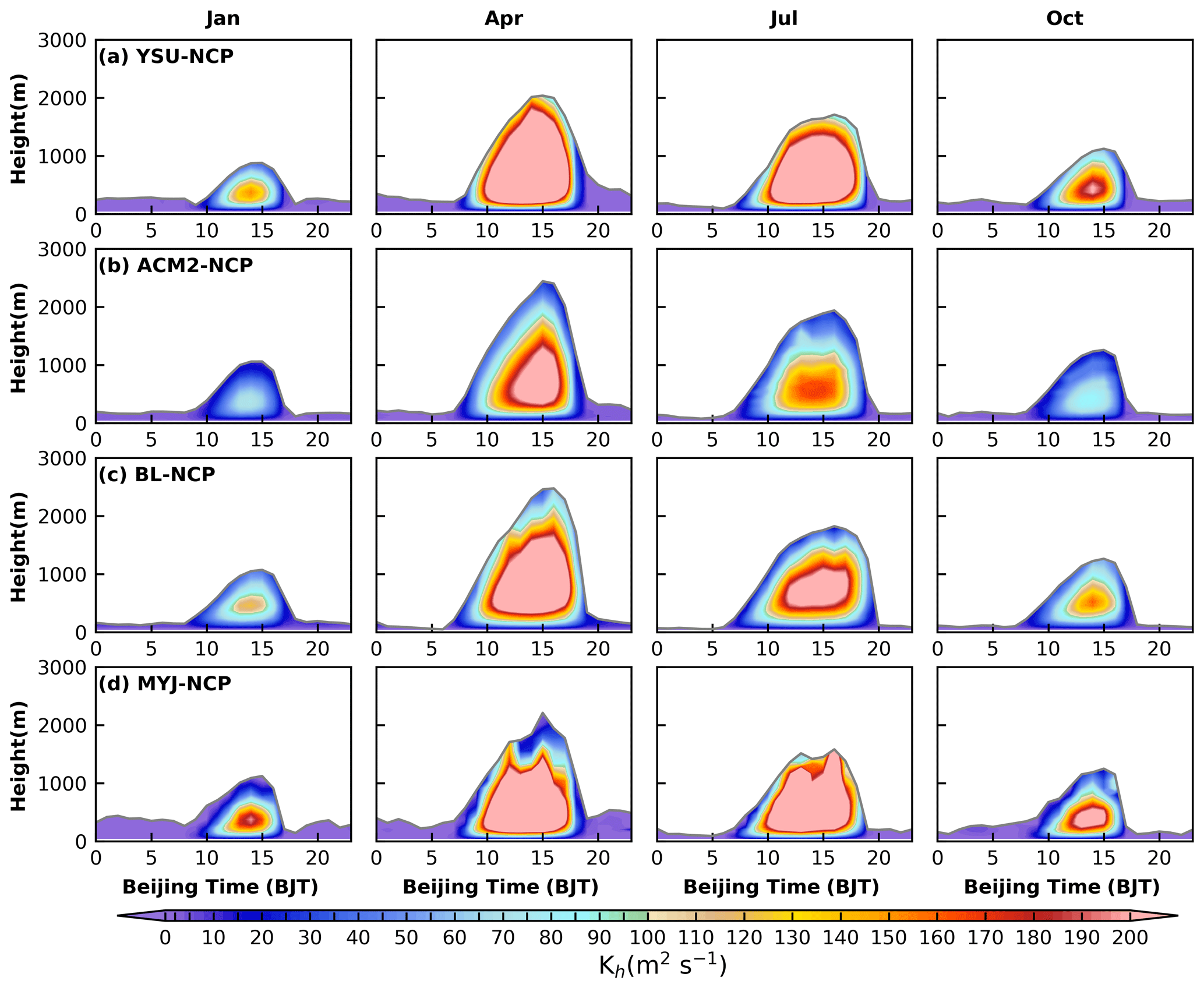
Figure 18 Time–height cross sections of heat turbulent diffusion coefficient simulated by (a) YSU scheme, (b) ACM2 scheme, (c) BL scheme, and (d) MYJ scheme for four seasons in the NCP region. The gray line indicates the PBLH.

From the Sect. 3.2.2 above, it is clear that the BL scheme has the strongest turbulent diffusion at 08:00 BJT, making the vertical gradient smaller, especially the wind speed is large. Similarly, this phenomenon can be found in the daily variation in turbulent diffusion, and not only at 08:00 BJT but almost throughout the night (Fig. 18). The difference between MYJ and BL schemes is mainly reflected in the calculation principle of mixing length, which is not directly related to the PBLH. In the BL scheme, mixing length scale can be relative to the distance that a parcel originating from this layer can travel upward and downward before being stopped by buoyancy effects (Eq. 14). Therefore, the vertical height below the temperature inversion layer at night, with the surface as the lower boundary, is the length scale of turbulence, i.e., mixing length scale. In the MYJ scheme, the mixing length scale is equal to z minus the integral depth scale, which is equal to the height of the equal-area rectangle under the profile. It is worth noting that the mixing length scale in the BL scheme mainly considers the effect of thermal and takes temperature gradient as the criterion, while the turbulent length scale in the MYJ scheme is mainly determined based on the TKE. TKE is further divided into horizontal TKE and vertical TKE. Horizontal TKE is mainly influenced by wind shear and the turbulent eddy scale can reach 1.5–3 times the PBLH on the horizontal and even reach 6 times the PBLH (Atkinson and Zhang, 1996). The vertical depth of an unstable layer capped by an inversion is automatically selected as the length scale for turbulence in the BL scheme during the daytime. Moreover, in the BL scheme, there is a counter-gradient correction term in the convective PBL, which leads to a downward transport of dry and cool air, making the thermal reach a lower height and a smaller length scale for turbulence (Bougeault and Lacarrere, 1989). We also find that the PBLH of the MYJ scheme exhibits a “sawtooth” and is more pronounced at night. This is mainly because the turbulence is weaker at night and presents intermittent characteristics, which, together with the judgment method of PBLH and the coarse vertical resolution, can cause such variation in the PBLH. Although the improvement of PBLH in the MYJ scheme cannot have a substantial effect on turbulent diffusion, the threshold value of its determination method is open to question.

3.5 Discussion of optimal PBL schemes

To better understand the simulation performance of different PBL parameterization schemes for different parameters in each region, this section will discuss the expressiveness of different PBL schemes through the statistical approach. Figure 19 shows the Taylor statistics for the analysis of near-surface meteorological parameters in 4 months in five regions.

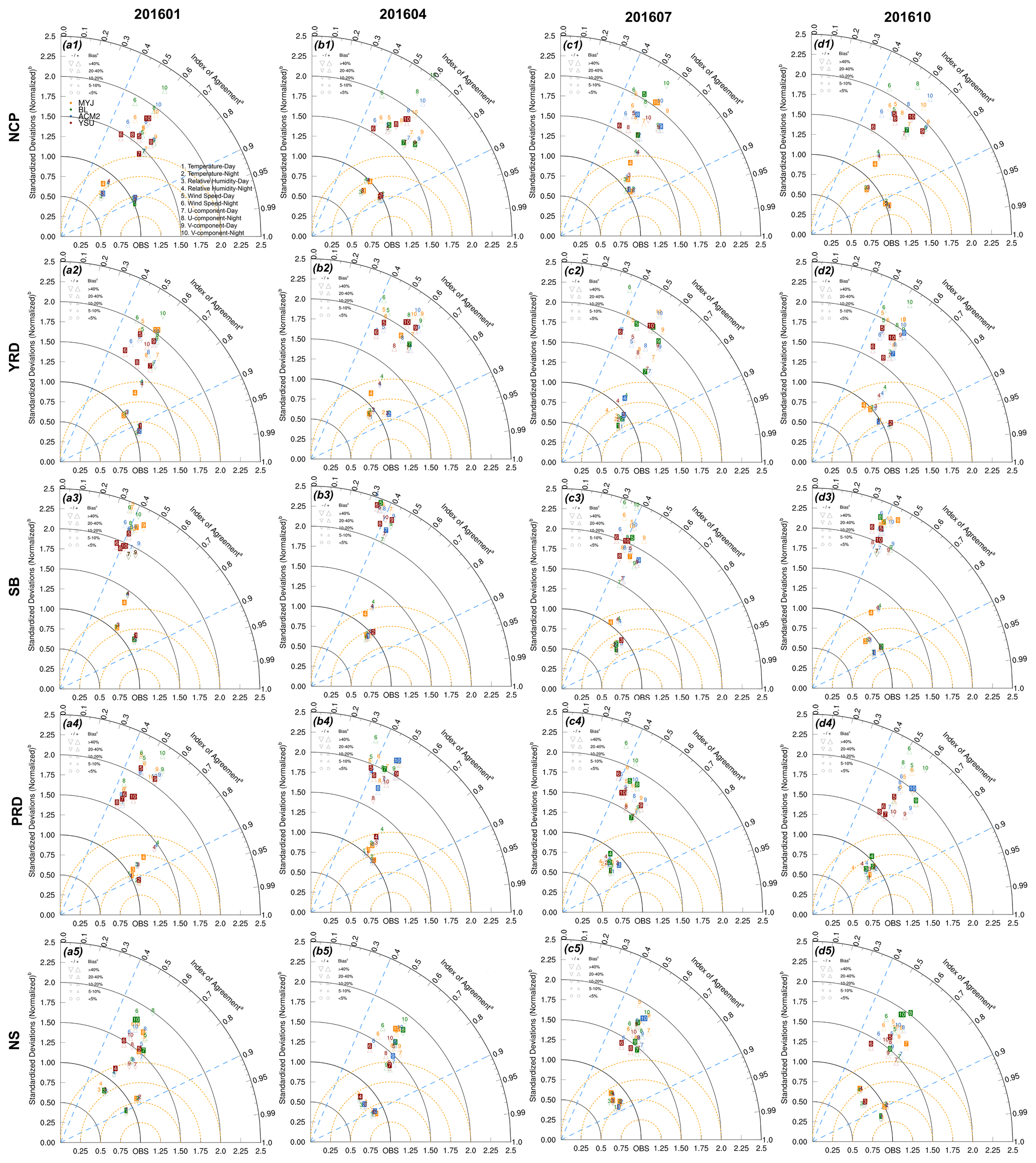
Figure 19 Taylor diagram of observation and simulation in five regions for four seasons. The x and y axes and arc represent the normalized standardized deviations (NSDs; $\mathrm{NSD}=\frac{\sqrt{\frac{\mathrm{1}}{N-\mathrm{1}}\sum _{i=\mathrm{1}}^n(X_{\mathrm{sim},i}-\stackrel{\mathrm{‾}}{X_{\mathrm{sim}}}{)}^{\mathrm{2}}}}{\sqrt{\frac{\mathrm{1}}{N-\mathrm{1}}\sum _{i=\mathrm{1}}^n(X_{\mathrm{obs},i}-\stackrel{\mathrm{‾}}{X_{\mathrm{obs}}}{)}^{\mathrm{2}}}}$, $\stackrel{\mathrm{‾}}{X_{\mathrm{sim}}}$ and $\stackrel{\mathrm{‾}}{X_{\mathrm{obs}}}$ represent the average value of simulation and observation, respectively) and index of agreement (IOA; $\mathrm{IOA}=\mathrm{1}-\frac{\left[\sum _{i=\mathrm{1}}^n\mathrm{|}{X}_{\mathrm{sim},i}-X_{\mathrm{obs},i}{\mathrm{|}}^{\mathrm{2}}\right]}{\left[\sum _{i=\mathrm{1}}^n(\left|X_{\mathrm{sim},i}-\stackrel{\mathrm{‾}}{X_{\mathrm{obs}}}\right|+\left|X_{\mathrm{obs},i}-\stackrel{\mathrm{‾}}{X_{\mathrm{obs}}}\right|{)}^{\mathrm{2}}\right]}$, X_sim,i and X_obs,i represent the simulated and observed values, respectively; i refers to time; and n is the total number of time series), respectively. Four schemes are shown in different colors, and different numbers represent different parameters. The root-mean-square error is denoted by the dashed orange line and the relative bias (RB; $\mathrm{RB}=\frac{\stackrel{\mathrm{‾}}{X_{\mathrm{sim}}}-\stackrel{\mathrm{‾}}{X_{\mathrm{obs}}}}{\stackrel{\mathrm{‾}}{X_{\mathrm{obs}}}}\times \mathrm{100}\mathit{\%}$) is shown by different symbols.

For the NCP region, the 2 m temperatures are underestimated during the daytime in January (Fig. 2), while the BL scheme simulates the highest temperature, meaning that the BL scheme performs optimally. Although the temperatures are somewhat overestimated at night, the overestimated period is shorter. The IOA of the four schemes is similar, with the ACM2 scheme having a slightly smaller bias (Fig. 19a1). Combined with the regional distribution of all stations in the NCP region, the BL scheme is recommended if the study area is mainly for Beijing, while the ACM2 and YSU schemes are recommended for the south of the NCP in January, such as Shandong Peninsula and southern Hebei province. For the other 3 months, temperatures are overestimated to varying degrees, both during the day and at night (Fig. 2). The MYJ scheme performs best in all statistical parameters at night (Fig. 19b1–d1), while during the daytime, it slightly underperforms the YSU and ACM2 schemes in relative bias in January and April, but the difference is not very distinct. Therefore, for the simulation of 2 m temperature in other 3 months, the MYJ scheme would be more recommended. In the YRD region, the 2 m temperatures are overestimated during the daytime, the BL schemes show overestimation at night, the MYJ scheme show underestimation, and the YSU and ACM2 schemes perform optimally (Fig. 2a2–d2). According to the Taylor statistical parameters, it can be seen that the ACM2 scheme performs better than the YSU scheme in the 4 months, and based on that the ACM2 scheme is recommended (Fig. 19a2–d2). The 2 m temperature in the SB region during the daytime is the same as in the YRD region, and the ACM2 scheme performs optimally (Fig. 19a3–d3). However, the BL scheme performs optimally during the nighttime, except in April (Fig. 19b3). The PRD region differs from the other regions in that the temperature simulation is significantly higher in January and April, and the MYJ scheme performs best in both daytime and nighttime (Fig. 19a4–b4). In contrast, the temperature simulation bias less in July and October, and the BL scheme performs best (Fig. 19c4–d4). The 2 m temperatures are almost underestimated during the daytime and overestimated for the nighttime in the NS region, and the MYJ scheme outperforms other schemes on account of its large diurnal temperature range (Fig. 19a5–d5). Of course, the BL scheme presents a slight advantage in the relative bias during the daytime in January (Fig. 19a5).

The results of 2 m relative humidity are relatively uniform, and the MYJ scheme shows optimal simulation performance in almost all months in all regions. Except for July in the YRD region, July and October in the PRD region, and January and April in the NS region (Fig. 19c2, c4–d4, a5–b5). For the simulation of 10 m wind speed and direction, the YSU scheme shows a very clear advantage, which is outstanding in all regions and all months (Fig. 19).

Several sounding stations with large differences between the observed and simulated altitudes are removed. Following this, the stations in each region are averaged to induce the variation characteristics from 100 to 2000 m in the vertical.

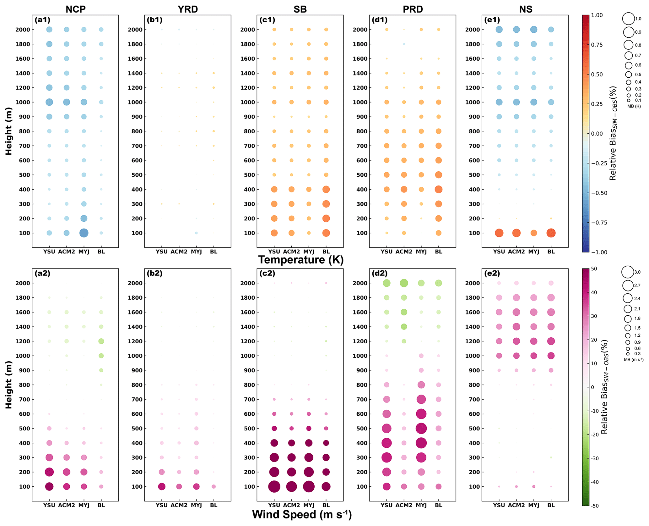
Figure 20 Statistics of temperature and wind speed in different layers at different vertical heights in January (winter), with circle size indicating the mean bias between simulations and observations, and circles filled with color denoting the relative bias.

The BL scheme has the smallest simulation bias for the temperature in the vertical direction in January for the NCP region, and performs optimally, which is associated with the discussion of the optimal scheme for the 2 m temperature (Fig. 20a1) to some degree. While in the other 3 months, the MYJ scheme has the smallest bias and is consistent with the conclusion of the 2 m temperature (Figs. S26–S28a1). In the YRD region, there is no clear difference between the four schemes for the simulation of temperature in the vertical direction, and the deviation of the simulation in January is less than 0.1 K (Fig. 20b1). The optimal scheme for 2 m temperature can be considered a representative choice. The MYJ scheme has a better simulation of the vertical profile of the temperature that is somewhat different from the most preferred scheme of 2 m temperature in the SB region (Figs. 20, S26–S28c1). This is mainly because the selected sounding stations are basically located in the basin area with low elevation, and the temperatures are overestimated, as is the 2 m temperature (Fig. 5). If the stations around the basin are not considered, the simulation of 2 m temperature will also be overestimated and the MYJ scheme also perform optimally. There is no complex topography in the PRD region, the results from the sounding stations and surface layer can be well echoed. In the vertical direction, the MYJ simulates the vertical profile of temperature better, particularly in January and April (Figs. 20, S30d1). While in July and October, the simulation results of the four schemes have little difference, especially in the lower level, which can be represented by the optimal scheme of 2 m temperature (Figs. S27–S28d1). For the NS region, there is an overestimation in the lower levels and an underestimation in the upper levels for each month. The height of overestimation is lower in January and April, around 200 m, while it can reach around 500 m in July and October (Figs. 20, S26–S28e1). The positive deviation decreases as the height increases, but after reaching a certain height, the negative deviation increases again. In the process of decreasing the positive deviation with height, the MYJ scheme performs the best, which is consistent with the 2 m temperature. While the BL scheme performs slightly better when the negative deviation gradually increases with height.

For wind speed, the YSU scheme is optimal for 10 m wind speed for all regions and months. However, they are quite different in terms of the variation in vertical wind speed. Throughout all regions and months, the simulation bias of the BL scheme is the smallest and closer to the observation, which is also the results obtained from the Sect. 3.2.2 (Figs. 20, S26–S28a2–e2). The stronger turbulent diffusion of the BL scheme at 08:00 BJT makes the wind speed more uniformly mixed in the vertical direction. The vertical variation characteristics at 08:00 BJT can be extended to the whole night. During the daytime, the result may not be the same, after all the vertical mixing of the YSU scheme is stronger and does not produce such a large wind speed gradient.

In general, in the selection process of the PBL scheme, if the focus is on temperature variation, such as temperature inversion, the optimal scheme for both 2 m temperature and vertical temperature can be considered, and there is basically no significant difference. However, if the focus is on the variation in wind speed and wind energy, then the vertical wind speed and that in the surface layer need to be evaluated and selected with comprehensive consideration.

4 Conclusions

The PBL serves as a bridge between the ground and the free atmosphere, and its role cannot be ignored. Turbulence, as the primary motion within the PBL, controls the vertical mixing of heat, water vapor, momentum, and pollutants. Turbulence as a sub-grid-scale motion is usually parameterized in the model, i.e., PBL parameterization scheme. The most widely used mesoscale model (i.e., WRF), which has developed 12 schemes, includes nonlocal closure scheme, local closure scheme and hybrid nonlocal-local closure scheme. Across the world, there have been many evaluation studies for PBL parameterization schemes (reference Fig. 1 in Jia and Zhang, 2020). However, most of the studies have been conducted for individual stations in a small region with special individual cases for research and analysis, which are not well represented and applied. Meanwhile, there is a deficiency in understanding the mechanism of the scheme itself. In response, aiming at the current research deficiencies, four typical schemes (YSU, ACM2, BL, and MYJ, covering each type scheme) are selected in this study to evaluate and analyze the near-surface meteorological parameters, vertical structure of the PBL, PBLH, and turbulence diffusion in 4 months (i.e., January, April, July, and October) in five typical regions of China (i.e., NCP, YRD, SB, PRD, and NS regions).

• a.

  The 2 m temperature. (1) In terms of time series and diurnal data, the simulation results for July are better than the other 3 months and better at night than daytime, with less deviation between simulation and observation. (2) In terms of regional distribution, temperatures at stations with higher elevations are easily underestimated (e.g., mountainous areas in the NCP region, areas around the SB basin, and the NS region) but overestimated at plains and basins (e.g., YRD, PRD, and the SB basin regions), and the overestimation and underestimation is more significant during the daytime. (3) In terms of mechanism differences between schemes, the differences in the simulated temperatures of the four schemes are more pronounced at night. The differences in simulated temperatures between the nonlocal scheme mainly originate from downward shortwave radiation, while the effects of sensible heat flux (HFX) need to be further ruminated when comparing them with the local closure scheme. When analyzing the HFX, the gradient of 2 m temperature and surface temperature, the variation in the heat transfer coefficient needs to be discussed in detail.

• b.

  The 2 m relative humidity. The changes in relative humidity and temperature correspond to each other, and again the best simulation results are obtained in July. With the exception of the NS region, the relative humidity of all regions is underestimated.

• c.

  The 10 m wind speed. (1) The simulation bias is the largest for the MYJ scheme during the daytime (except for the NCP region), the BL scheme presents the largest deviation at night in all regions, and the difference is not significant in the 4 months. The variation in 10 m wind speed is influenced by the momentum transfer coefficient, where a larger C_m produces stronger mixing and transports more momentum from the upper layers to the lower layers. For the YSU, ACM2, and BL schemes, the C_m and 10 m wind speed vary proportionally. In contrast, the MYJ scheme is different from the other schemes, and the C_m is larger than other months almost all day. However, the wind speed simulated by the MYJ scheme is at its maximum only during the daytime, which indicates that it is influenced by integrated similarity functions. (2) In terms of regional distribution, the wind speed is more overestimated in plains and basins and less overestimated or even underestimated in mountainous areas. This is chiefly due to the influence of the model on terrain smoothing. (3) The overestimation of smaller wind speed at night is more obvious in the four schemes, primarily owing to the non-application of the MOST. At night, the turbulence intensity is disproportionate to the mean gradient, and the M-O similarity theory is no longer applicable.

• d.

  The 10 m wind direction. The simulation of wind direction in January for the NCP region worse than the other 3 months, and the frequency of simulated northwesterly and northerly winds is overestimated by about 6.6 %. For the YRD region, the frequency of northeasterly winds is overestimated. The simulation of wind direction in the SB region is not as good as other regions due to the complex topography. The frequency of northeasterly winds is overestimated in January and October in the PRD region, and that of southerly winds is overestimated in April and July. The wind direction is better simulated for the NS region, and the difference is not very obvious.

• e.

  PBL vertical structures. The model can reproduce the vertical structure of temperature well, but the inversion temperature at the lower levels of many stations in complex terrain cannot be simulated well, mainly because there is a certain difference in the terrain height between observation and simulation. At 08:00 BJT, the MYJ scheme simulates the lowest temperature and the BL scheme for the highest temperature, and the difference is more conspicuous at the lower levels. The vertical structure of the wind speed is clearly not as good as the temperature. The wind speed is almost always overestimated below 1000 m, except for the NS region. Unlike the 10 m wind speed, YSU has the smallest deviation from the 10 m wind speed, while the BL scheme has the smallest bias in the vertical direction. The BL scheme has the largest turbulent diffusion and the strongest mixing at 08:00 BJT.

• f.

  PBLH. The PBLH values calculated based on the observed data using the two methods are better in January than in the other 3 months and in the NCP region than in the other four regions. The wind speed gradient simulated by the YSU scheme is large, resulting in a small Richardson number (Ri), making the height higher when Ri reaches 0.25 and the PBLH is higher than that of the ACM2 scheme. The PBLH simulated by the BL scheme is closer to the observation because the temperature gradient is best simulated. The MYJ scheme results in a jagged variation in the PBLH due to the determination of the threshold and the vertical resolution, and this phenomenon is especially obvious at night. In terms of regional distribution, the PBLH is best simulated in the YRD region, followed by the PRD region, and is worst in the NS region. The results are similar in January and October, when the PBLH is lower and the simulations are better than those in April and July.

• g.

  Turbulent diffusion coefficient. (1) The TDC simulated by the YSU and MYJ schemes is the largest during the daytime, followed by the BL scheme, and the smallest in the ACM2 scheme. The TDC simulated by the BL scheme is the largest at night, and the other three schemes are about the same. (2) The TDC is maximum in April and July and minimum in January and October. (3) The obvious difference in PBLH affects the turbulent diffusion of the YSU and ACM2 schemes. It is worth noting that the YSU scheme calculates the TDC of momentum first and then uses Prandtl number (Pr) to calculate the TDC of heat, while the ACM2 scheme calculates the TDC of both momentum and heat. (4) The difference between the BL and MYJ schemes is mainly reflected in the calculation principle of mixing length. The buoyancy effect mainly affects the mixing length scale in the BL scheme, and the mixing length scale of MYJ scheme is influenced by the TKE.

For the discussion of the optimal scheme, different schemes need to be proposed for different parameters. (1) The first is temperature, where the BL scheme is recommended for January in the NCP region, especially for Beijing, and the MYJ scheme is recommended for the other 3 months. The simulation difference between the four schemes is small in the YRD region, and the ACM2 scheme is recommended. The topography is more complex in the SB region, but the MYJ scheme is recommended for most areas within the basin, and the BL scheme is recommended for the SB region if more area around basin is involved. The MYJ scheme is recommended for the PRD region in January and April, and the BL scheme is recommended for July and October. In the NS region, the MYJ scheme is recommended. (2) The second parameter is relative humidity, where the MYJ scheme is recommended for all regions in 4 months. (3) The third parameter is wind speed, where the YSU scheme is recommended if the main concern is the surface layer, and the BL scheme is recommended if the focus is on the variation in wind speed in the vertical direction.

The PBL parameterization scheme, as the most critical parameterization process within the PBL in the model, has been proposed and developed well by previous generations, but the development has been slower in recent years, as few new theories have been proposed, almost no new schemes have been put into the model, and the existing schemes have rarely been improved. Most of the previous studies have evaluated the PBL parameterization scheme, but many of them focus on a particular case in a certain region and lack of universality. This study makes up for this deficiency and provides a comprehensive discussion on the evaluation and uncertainty analysis of the PBL parameterization scheme, hoping to give some reference to the model users. The future development of the PBL parameterization scheme needs to start from the theoretical mechanism, go deeper into the PBL parameterization scheme, and have a deeper understanding of the PBL parameterization, even if it is only for one scheme, or the improvement of one parameter. As for the GRAPES model, which was developed independently in China, the introduction and improvement of PBL parameterization schemes need to be screened, rather than introducing all the schemes into the GRAPES model at once, and in fact many schemes have hardly been tested and used.