the Creative Commons Attribution 4.0 License.
the Creative Commons Attribution 4.0 License.
 | 24 Nov 2023
Comprehensive evaluation of typical planetary boundary layer (PBL) parameterization schemes in China – Part 2: Influence of uncertainty factors
Wenxing Jia
Xiaoye Zhang
Hong Wang
Yaqiang Wang
Deying Wang
Junting Zhong
Wenjie Zhang
Lei Zhang
Lifeng Guo
Yadong Lei
Jizhi Wang
Yuanqin Yang
Yi Lin
This study focuses on the uncertainties that influence numerical simulation results of meteorological fields (horizontal resolution: 75, 15, and 3 km; vertical resolution: 48 and 62 levels; near-surface (N-S) scheme: MM5 and Eta schemes; initial and boundary conditions: Final (FNL) and European Center for Medium-Range Weather Forecasting (ECMWF) reanalysis data; underlying surface update: model default and latest updates; model version: version 3.6.1 and 3.9.1). By further evaluating and analyzing the uncertainty factors, it is expected to provide relevance for those scholars devoted to factor analysis in order to make the results closer to the observed values. In this study, a total of 12 experiments are set up to analyze the effects of the uncertainties mentioned above, and the following conclusions are drawn: (1) horizontal resolution has a greater effect than vertical resolution; (2) the simulated effects of temperature and wind speed in the N-S scheme are smaller than those in the planetary boundary layer (PBL) scheme; (3) the initial and boundary conditions of different products have the most remarkable effect on relative humidity, while the simulation results of ECMWF data are the best; (4) the updates with urban and water bodies as the underlying surface have a more significant contribution to the meteorological fields, especially on temperature; and (5) for the PBL parameterization schemes, the update of the model version has less impact on the simulation results because each update has small changes and no major changes overall. In general, the configuration of uncertainties needs to be considered comprehensively according to what you need in order to obtain the best simulation results.
- Article
(44722 KB) - Full-text XML
- Companion paper
-
Supplement
(6083 KB) - BibTeX
- EndNote


The key factor for the accurate simulation of near-surface (N-S) meteorological parameters and planetary boundary layer (PBL) structures is the PBL parameterization scheme. Part 1 discussed the impact of the PBL schemes in detail from the mechanism and assessed the applicability of the PBL schemes for different parameters (i.e., 2 m temperature, 2 m relative humidity, 10 m wind speed and direction, PBL vertical structures, PBL height, turbulent diffusion coefficient) in different regions (i.e., North China Plain, NCP; Yangtze River Delta, YRD; Sichuan Basin, SB; Pearl River Delta, PRD; and the Northwest Semi-arid region, NS) and seasons (i.e., January, April, July, and October) (Jia et al., 2023). However, there are still many uncertainties in the model that can affect the forecasts and model results. The model settings used by different scholars exhibit differences in the simulation results. For example, the horizontal and vertical resolutions are essential for model settings. Horizontal resolution, as a critical factor, must be considered in all models, whether they are macroscale Earth system models (Ma-ESMs), climate models (CMs), mesoscale weather models (Me-WMs), or microscale fluid models (Mi-FMs). Constrained by computational resources, a horizontal resolution of about 100–250 km is used for Ma-ESMs models (e.g., Coupled Model Intercomparison Project phase 6, CMIP6 model) (Li et al., 2022; Taylor et al., 2012). The horizontal resolution of CMs typically ranges from 50 to 25 km (e.g., Flexible Global Ocean-Atmosphere-Land System Finite-Volume version 3, FGOALS-f3 model) (Li et al., 2021). The horizontal resolution of Me-WMs (e.g., the Global/Regional Assimilation Prediction System model, GRAPES, and the Weather Research and Forecasting model, WRF) (García-García et al., 2022; Ma et al., 2018) can be as fine as 1 km. The Mi-FMs can have a horizontal resolution of less than 100 m (e.g., large eddy simulation model, LES) (Zhou et al., 2017). Studies have shown that the interaction between large and small-scales is influenced by resolution, with finer resolution allowing for better characterization of underlying surface features and extreme events (Rummukainen, 2016; Singh et al., 2021) and also impacting future climate predictions (Chang et al., 2020; Roberts et al., 2020; Small et al., 2014). The use of PBL scheme is usually in coarse-resolution models, which can lead to additional errors since these schemes are developed for flat terrain conditions (Weigel et al., 2007).
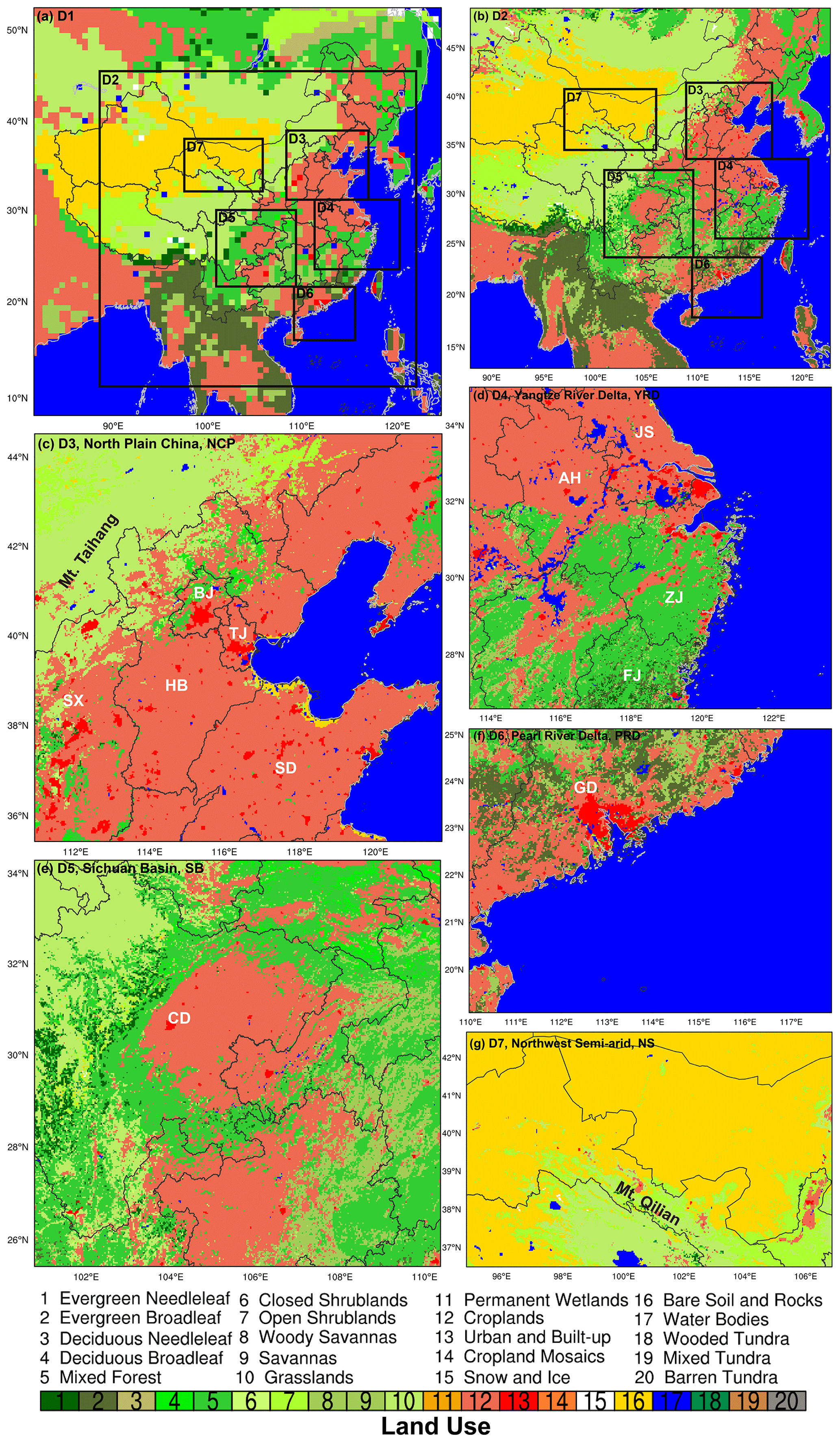
Figure 1(a–g) Map of land use type in the seven nested model domains. The abbreviations BJ, TJ, HB, SX, SD, JS, ZJ, AH, FJ, CD, GD, Mt. Taihang, and Mt. Qilian denote the Beijing municipality, Tianjin municipality, Hebei province, Shanxi province, Shandong province, Jiangsu province, Zhejiang province, Anhui province, Fujian province, Chengdu municipality, Guangdong province, Taihang mountains, and Qilian mountains in panels (c)–(g), respectively.
Finer vertical resolution can better capture changes in PBL structures, which can also have an impact on mass transport (Menut et al., 2013; O'Dea et al., 2017; Teixeira et al., 2016), especially on the accuracy of wind resources (Tolentino et al., 2016). In addition, horizontal and vertical resolutions can cause spurious gravity waves and increase model errors (Nolan and Onderlinde, 2022). Although finer resolution is better, there is no doubt that it is computationally expensive. Whether the use of finer resolution will bring significant improvement to the model results deserves further discussion.
Different PBL schemes are combined with the different N-S schemes, both of which are crucial to the simulation results of the meteorological fields (Jia and Zhang, 2020). For instance, the Mellor–Yamada–Janjić (MYJ) PBL scheme can only couple the Eta N-S scheme, while the Bougeault and Lacarrere (BL) PBL scheme can couple both the MM5 and the Eta N-S schemes. The N-S scheme is pivotal for mesoscale numerical simulation, especially for fine numerical forecasting (Li et al., 2010). Then, to figure out which scheme has a greater impact on the meteorological field will help to make targeted improvements to the forecasts in the future.
In addition, the lag of the underlying surface data can also affect the simulation results of the meteorological fields, especially for large cities with relatively rapid urbanization (Qian et al., 2022). In particular, different underlying surface conditions can have different albedos that affect the temperature changes, which can affect the urban heat island effect from a local perspective and global warming from a global perspective (Ouyang et al., 2022; Schwaab et al., 2021; Wang and Li, 2021).
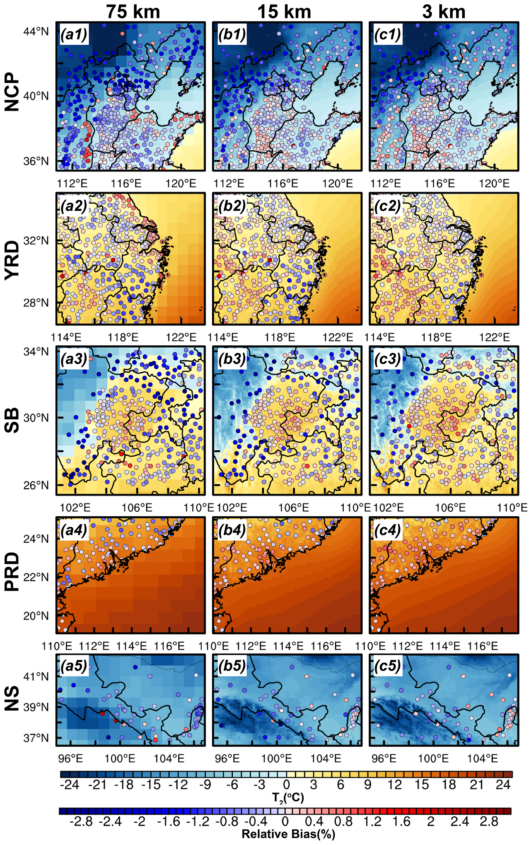
Figure 2Regional distribution of 2 m temperature simulated by (a) domain 1 (75 km), (b) domain 2 (15 km), and (c) domain 3 (3 km) for five regions in January, and distribution of relative bias between simulations and observations is denoted by scatters.
The most commonly used final (FNL) reanalysis dataset is jointly produced by the National Centers for Environmental Prediction (NCEP) and the National Center for Atmospheric Research (NCAR). They have adopted a global data assimilation system and a well-established database for quality control and assimilation of observations from various sources (ground, ships, radio soundings, wind balloons, aircraft, satellites, etc.) to obtain a complete set of reanalysis dataset. The European Center for Medium-Range Weather Forecasting (ECMWF, hereafter referred to as EC) has concluded that the steady progress in numerical forecasting over the last 30 years is mainly attributed to improvements in the forecast models themselves, the application of more observations, and the development of data assimilation techniques (Magnusson and Källén, 2013). Among these examples, the performance of the forecast model depends largely on the model resolution, the accuracy of the finite-difference method, and the representativeness of the physical process parameterization scheme. Different initial fields also influence the model results due to different observational data, quality control methods, assimilation schemes, and bias correction methods adopted for different reanalysis data (Ma et al., 2021).
Finally, we also have to take the update of the model version into account. With model versions being updated, many parameterization schemes are more or less updated (Morichetti et al., 2022). However, under the circumstance that the updates are not disclosed in scientific and technical reports or papers, we need to dig into them from the code itself. In reality, simulation results will be likely to vary from scholar to scholar because of the different model versions they choose (Jia and Zhang, 2020). Consequently, it is necessary to adopt a control variable approach when discussing the impact of model version updates. Instead of updating all parameterization schemes, only by updating the ones we are concerned with can the uncertainty arising from version updates can be quantified.
Table 1Detailed parameter settings of the 12 experiments.
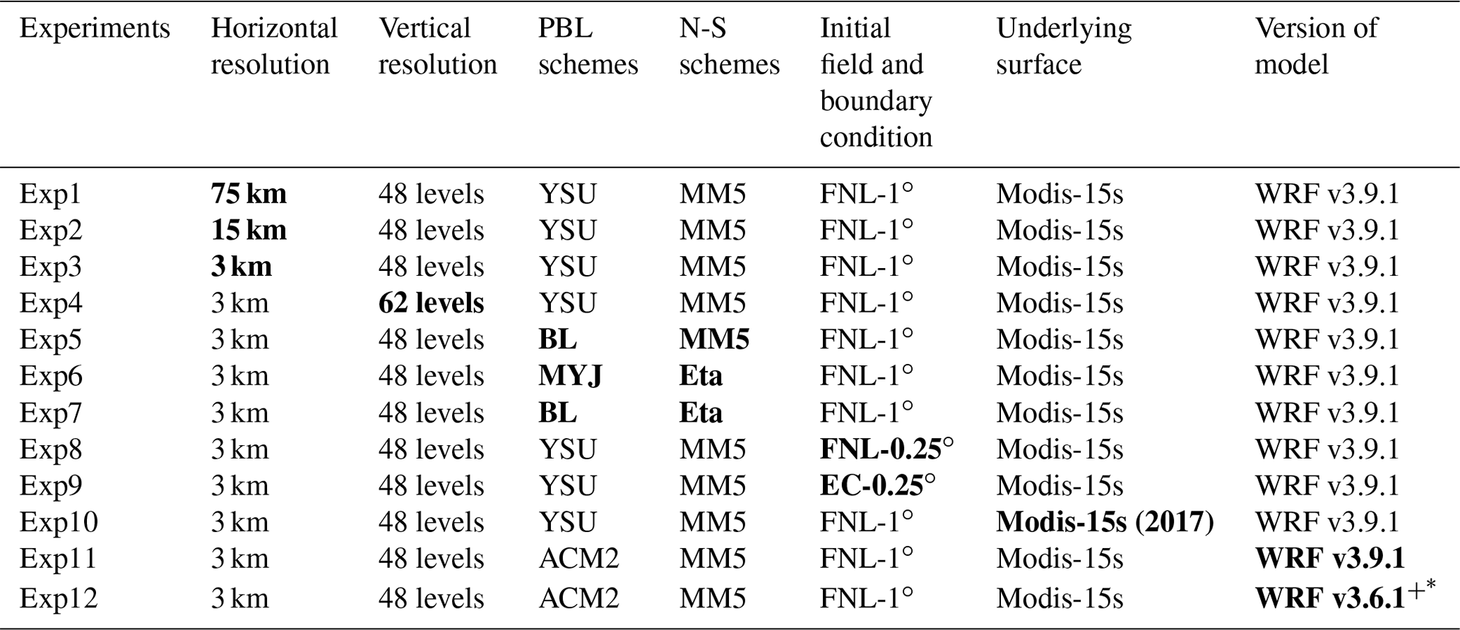
* WRF3.6.1+ refers to the migration of the ACM2 scheme from WRFv3.6.1 to WRFv3.9.1, ensuring that there are no changes in other parameterization schemes. Bold text indicates uncertainties of primary concern.
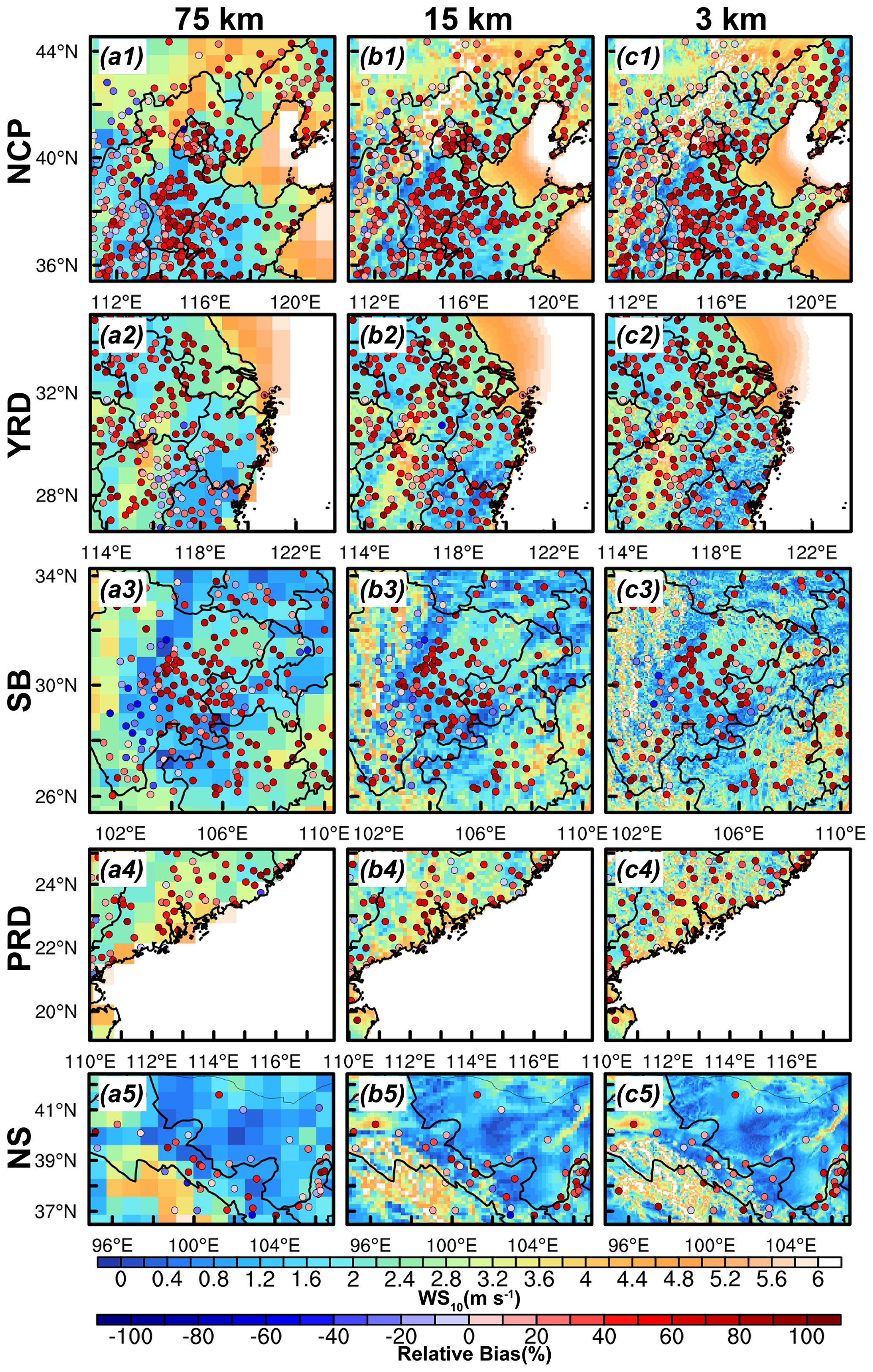
Figure 3Similar to Fig. 2 but for 10 m wind speed.
These aforementioned uncertainties have been studied by scholars individually, but few scholars have been able to synthesize and analyze these factors. In this part (i.e., Part 2), each of these uncertainties will be analyzed and discussed, and the factors with more significant effects will be selected for reference as identifying which factors besides the PBL scheme are critical to the simulation of meteorological fields makes all the difference.
2.1 Data
2.1.1 Reanalysis data
Final (FNL) reanalysis data. The NCEP global FNL reanalysis data are based on the 6 h temporal resolution (i.e., 00:00 (08:00), 06:00 (14:00), 12:00 (18:00), 18:00 UTC (02:00 BJT)) by the Global Data Assimilation System (GDAS) with a resolution of or . This product continuously collects observational data from the Global Telecommunications System (GTS) and other sources. The FNL reanalysis data are made with the same model as NCEP uses in the Global Forecast System (GFS), but the FNL reanalysis data are prepared about an hour or so after the GFS is initialized. The FNL reanalysis data parameters include surface pressure, sea level pressure, geopotential height, temperature, sea surface temperature, soil values, ice cover, relative humidity, winds, vorticity, etc. The data temporal range for 1∘ is from 30 July 1999 to the present (https://doi.org/10.5065/D6M043C6, National Centers for Environmental Prediction/National Weather Service/NOAA/U.S. Department of Commerce, 2000), while the time range for the 0.25∘ is from 8 July 2015 to the present (https://doi.org/10.5065/D65Q4T4Z, National Centers for Environmental Prediction/National Weather Service/NOAA/U.S. Department of Commerce, 2015).
The fifth-generation ECMWF reanalysis (ERA5) data. The ERA5 is the fifth-generation EC reanalysis of the global climate. Reanalysis combines model data with observations worldwide to form a globally complete and consistent dataset. ERA5 replaces its predecessor, the ERA-Interim reanalysis. ERA5 data are available from 1959 to present with a resolution of (atmosphere) and (ocean waves). The model requires 3D data and 2D data, and the variables of 3D data are temperature and U and V components of wind, geopotential height, and relative humidity (https://cds.climate.copernicus.eu/cdsapp#!/dataset/reanalysis-era5-pressure-levels?tab=overview, last access: 22 November 2023). The 2D data mainly include the parameters surface pressure; mean sea level pressure; skin temperature; 2 m temperature; 2 m relative humidity; and 10 m U and V components of wind, soil data, and soil height (https://cds.climate.copernicus.eu/cdsapp#!/dataset/reanalysis-era5-single-levels?tab=overview, last access: 22 November 2023).
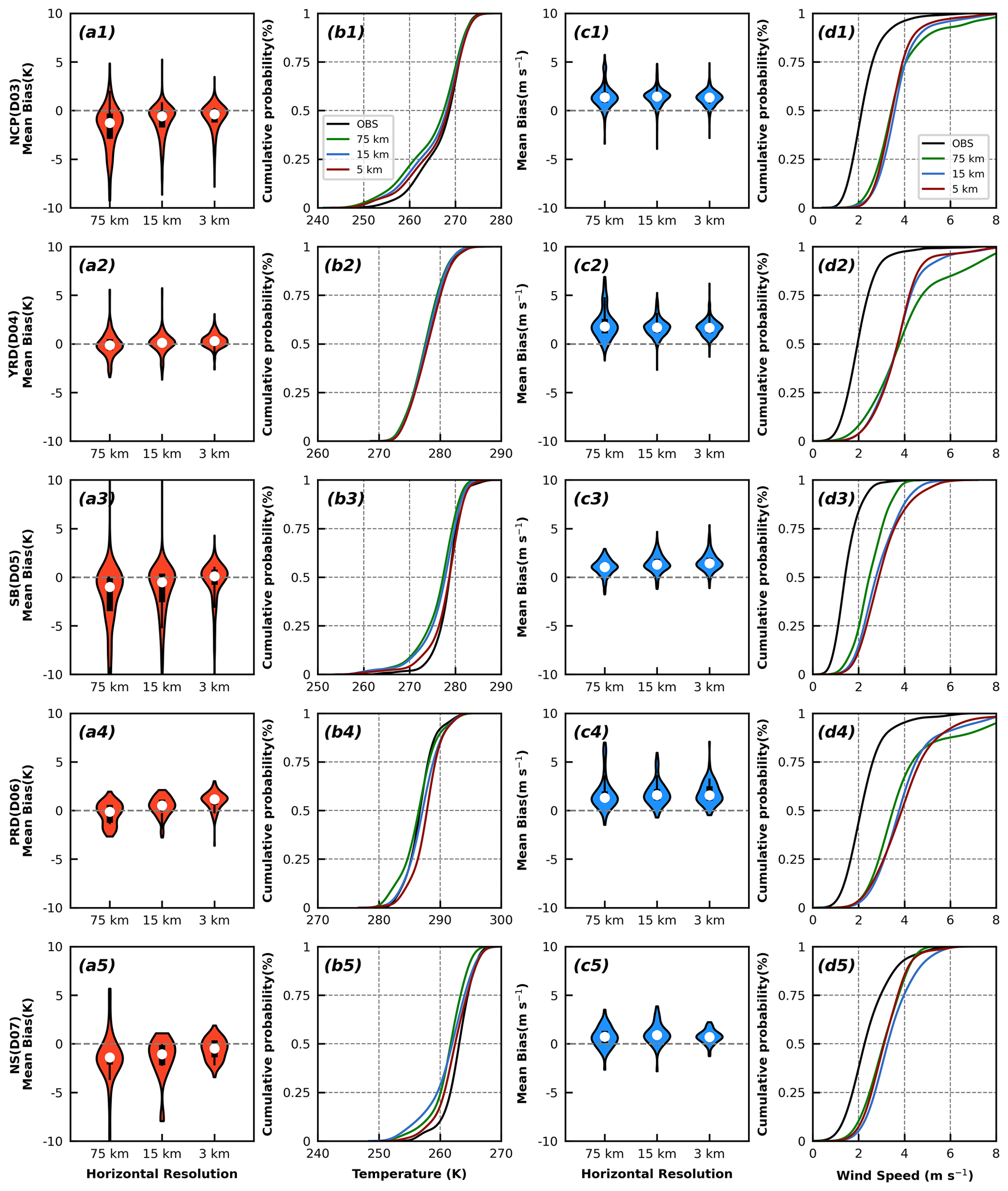
Figure 4Violin plots of mean bias of observed and simulated (a1–a5) 2 m temperature and (c1–c5) 10 m wind speed at different horizontal resolutions (i.e., 75, 15, 3 km) and the cumulative probability of observed and simulated (b1–b5) 2 m temperature and (d1–d5) 10 m wind speed at different horizontal resolutions (i.e., 75, 15, 3 km) for five regions.
2.1.2 Underlying surface data
The default underlying surface data in WRF are USGS and MODIS data, where USGS has 24 classifications and MODIS has 20 classifications. In this study, MODIS data is selected. The basic land cover is a modified International Geosphere Biosphere Programmer (IGBP), which is calculated by supervised classification using MODIS Terra and Aqua reflectance data, with a resolution of 500 m (https://www2.mmm.ucar.edu/wrf/users/download/get_sources_wps_geog.html, last access: 22 November 2023). The dataset that comes with WRF is based on the year 2001 (Bhati and Mohan, 2016). The 20 types are evergreen needleleaf, evergreen broadleaf, deciduous needleleaf, deciduous broadleaf, mixed forest, closed shrublands, open shrublands, woody savannas, savannas, grasslands, permanent wetlands, croplands, urban and built-up, cropland mosaics, snow and ice, bare soil and rocks, water bodies, wooded tundra, mixed tundra, and barren tundra.
To consider the influence of the underlying surface data on the model results, we further select the same underlying surface data as the simulation period (i.e., January 2016) (https://e4ftl01.cr.usgs.gov/MOTA/MCD12Q1.061/, last access: 22 November 2023). These data are the MCD12Q1 version 6 data product (Friedl et al., 2002), including 17 land types that cover the IGBP land cover classification.
2.2 Description of the modeling experiments
The regional settings and basic settings of the model are the same as those in Part 1, focusing on the same five regions, and the month selected as the test time is January. To evaluate the effect of these uncertainties on the simulation results of the meteorological fields, a total of 12 experiments are conducted, and the detailed configuration of the experiments is shown in Table 1. The effect of horizontal resolution is presented by three experimental comparisons in Exp1, Exp2, and Exp3, and the effect of vertical resolution is shown in Exp3 and Exp4. The implications of the surface layer schemes are analyzed by comparing three experiments in Exp5, Exp6, and Exp7. The impact of the initial field and boundary conditions are compared by three experiments, i.e., Exp3, Exp8, and Exp9. The influences of the underlying surface are displayed by Exp3 and Exp10. The update of the model version is compared by Exp11 and Exp12.
3.1 horizontal resolution impact on 2 m temperature and 10 m wind speed
The underlying surface information is crucial to the simulation of near-surface meteorological parameters. From the distribution of the underlying surface, the three different resolutions of the model can basically capture the general information of the underlying surface (Fig. 1). The resolution of 75 km is relatively coarse, so many fine features are ignored and represented uniformly by a large grid (Fig. 1a). The resolution of 15 km is significantly different compared to 75 km (Fig. 1b), and many fine characteristics (e.g., lakes, cities, etc.) are represented that are very close to the features of the 3 km resolution.
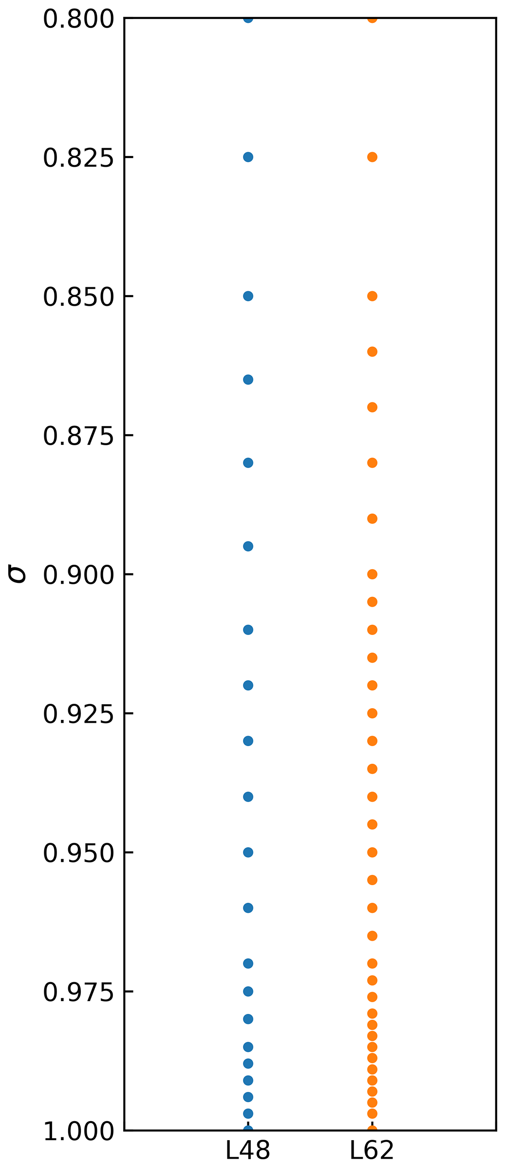
Figure 5Vertical level distributions for the two experiments with σ below 2 km in the model.
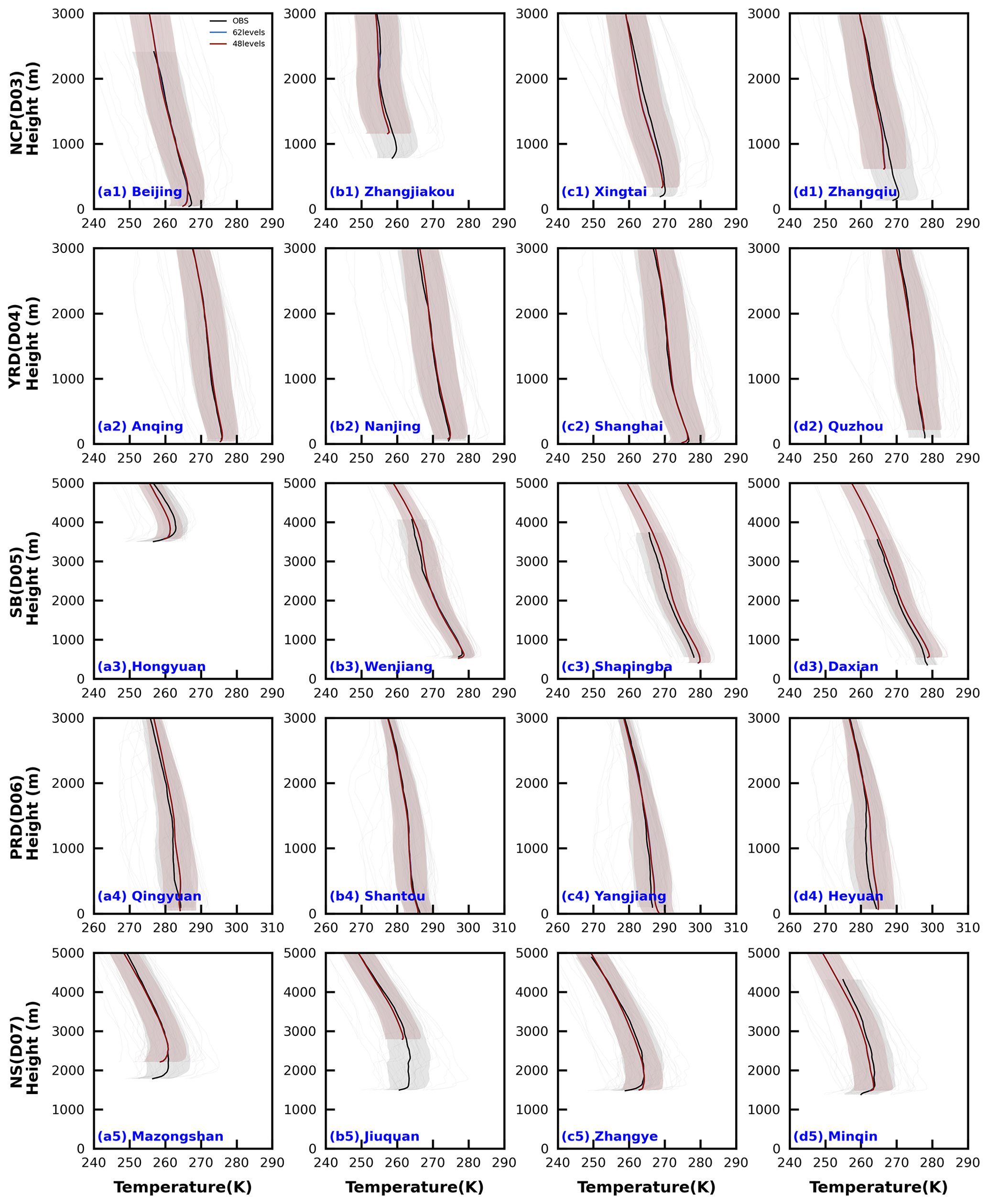
Figure 6Average vertical profiles of observed and simulated temperature at 08:00 and 20:00 BJT at four sounding stations for each region in January. The transparent gray lines indicate the simulated lines for all time periods, the lines with shading indicate the average values, and shaded areas show the uncertainty range (the mean ±1 standard deviation).
Further comparative analyses of temperature and wind speed have been performed in five regions at these three resolutions. In terms of regional distribution, all three experiments can simulate high- and low-value areas of 2 m temperature, but there are differences in the degree of overestimation and underestimation (Fig. 2). In the NCP region, the three experiments underestimate the temperature over a similar range of regions, especially in the northwest (Fig. 2a1–c1). Exp1 differs more sharply from the other two experiments in areas with more marked underlying surface variability, such as in the complex mountainous areas (i.e., Taihang mountains, Mt. Taihang) in the northwest, the underestimation of Exp1 is more significant, but at the sea–land interface, the overestimation of Exp1 is more pronounced (Fig. 2a1) because the grid resolution is too low. The number (N) of stations overestimated by the three experiments is 96, 128, and 172, and the relative bias (RB) values are 0.38 %, 0.19 %, and 0.18 %, respectively. Although the number of stations overestimated by Exp1 is small, there are more extreme values, which means that the deviation is larger. Correspondingly, the higher degree of underestimation (−0.89 %) in Exp1 derives from more minimal values and stations (N=397) as well. For the YRD region, Fig. 2a2–c2 note that the RB of the stations varies greatly with different horizontal resolutions, especially for the northeastern coast of the YRD region (i.e., northeastern Jiangsu (JS) province) from overestimation (Fig. 2a2) to underestimation (Fig. 2c2), and the degree of underestimation gradually decreases in the southeast of YRD (i.e., Zhejiang (ZJ) and Fujian (FJ) provinces). In the SB region, it is clear that Exp1 underestimates the 2 m temperature more significantly (RB , N=245), with fewer stations in the Fig. 2a3; this is followed by Exp2 (RB , N=208) and to a lesser extent by Exp3 (RB , N=152). The PRD region behaves differently from other regions, with the simulation results of Exp1 showing an underestimation (RB ), while Exp2 (RB =0.13 %) and Exp3 (RB =0.35 %) show an overestimation (Fig. 2a4–c4). The variation in the underlying surface between grids in the PRD region is more complex in comparison with other regions (Fig. 1). This does not indicate that the simulation results are better when the grid horizontal resolution is lower because the scheme itself still has errors in the simulation. It only reveals that the simulation results of Exp1 perform better statistically in the current model configuration for this region. The number of stations in Exp1 in the NS region is much lower than the other two experiments, which means that the relative bias of Exp1 is more than ±3 % and the deviation is greater for the area along the Qilian mountains (Mt. Qilian) (Fig. 2a5–c5) in particular.
The results of wind speed are different from those of temperature, and the difference between the three experiments is not as obvious as that of temperature (Fig. 3). The three experiments overestimate the wind speed to varying degrees; however, more stations underestimate wind speed in the Exp1, especially in the NCP (NExp1=34, NExp2=21, NExp3=19) and SB regions (NExp1=29, NExp2=18, NExp3=7) (Fig. 3a3). As the grid resolution is too coarse in Exp1, the wind speed is underestimated at some stations due to the complex terrain in the NCP and SB regions (Fig. 3a1, a3).
It can also be seen from Fig. 4 that the three experiments have a large difference in temperature simulation, and the underestimation in Exp1 is more significant (Fig. 4a1–a5). However, in the PRD region, the average value of the mean bias is closer to 0 on account of the offsetting positive and negative deviations. For the distribution range of the mean bias, it has been found that the distribution of the Exp1 is closer to 0 (Fig. 4a4). In terms of the cumulative probability distribution, the simulations differ for different temperature segments in the NCP, SB, and NS regions. For the NCP region, the temperature below 270 K is better simulated in Exp3, the temperature threshold in the SB region is about 280 K, and the threshold is about 265 K in the NS region (Fig. 4b1, b3, b5). In the YRD region, the simulations of all three experiments are almost the same for any segmented temperature (Fig. 4b2). In addition, the PRD region is special, with temperature below about 285 K, and the Exp2 simulates this better (Fig. 4b4). It is worth noting that, regardless of the region, one common element is that the temperature of the simulations in the three experiments gets closer and closer as the temperature increases. However, the difference in wind speed between the three experiments is not obvious (Fig. 4c1–c5). The average value of the mean bias in Exp1 is closer to 0, mainly attributable to the fact that there are more stations with negative mean bias to offset. Wind speed and temperature behave differently in regard to cumulative probability distributions, with increasing differences in simulated wind speeds for the three experiments as wind speed increases (Fig. 4d1–d5). The wind speed simulated in Exp1 is low, leading to a better performance in Exp1 for low wind speed (Fig. 4d1–d5).
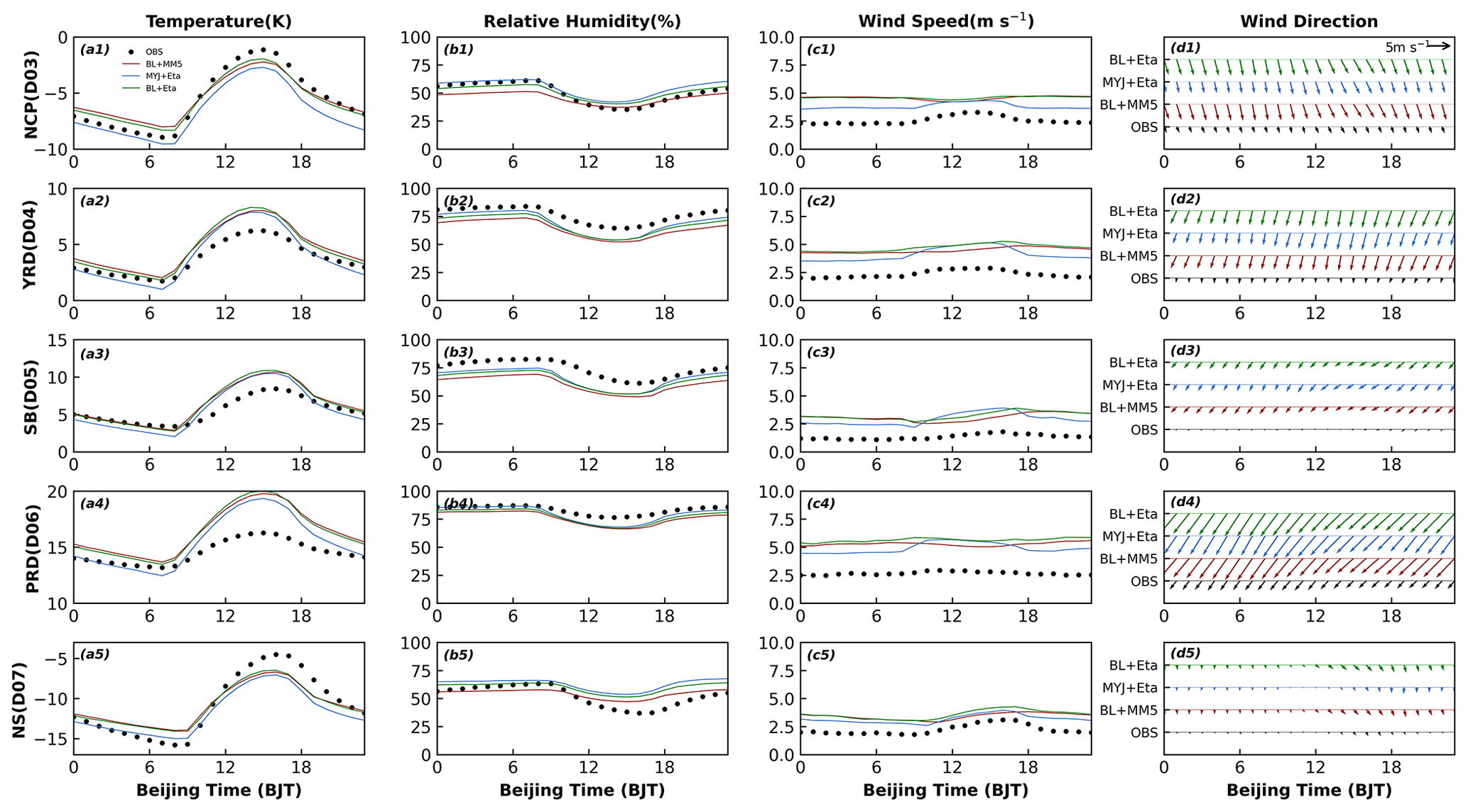
Figure 8Time series of diurnal variation of (a1–a5) 2 m temperature, (b1–b5) 2 m relative humidity, (c1–c5) 10 m wind speed, and (d1–d5) 10 m wind direction for five regions in January.
3.2 Vertical resolution impact on PBL structures
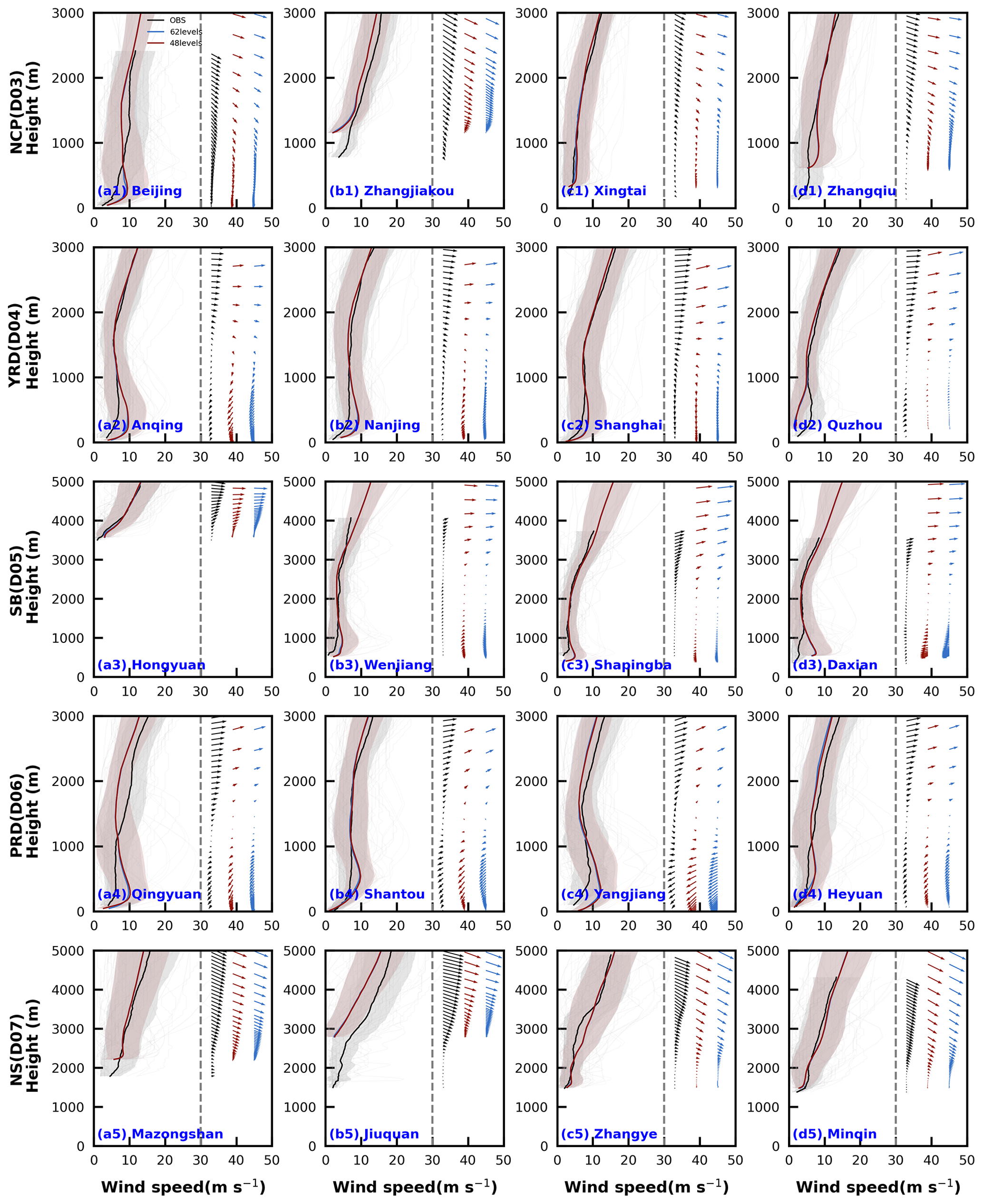
Based on Exp3, the vertical resolution has been further encrypted from 21 to 35 levels below 2 km, i.e., the total number of vertical levels is increased from 48 to 62 levels (Fig. 5). The temperature and wind fields of the two experiments (Exp3 and Exp4) simulations are compared for the four sounding stations selected for each region in Part 1 (NCP: Beijing, Zhangjiakou, Xingtai, and Zhangqiu; YRD: Anqing, Nanjing, Shanghai, and Quzhou; SB: Hongyuan, Wenjiang, Shapingba, and Daxian; PRD: Qingyuan, Shantou, Yangjiang, and Heyuan; NS: Mazongshan, Jiuquan, Zhangye, and Minqin). As can be seen from Fig. 6, the re-encryption of the vertical resolution has no effect on the simulation of the temperature, regardless of the region. The simulation results of the two experiments almost overlap in the vertical direction, implying that the vertical structure of 48 levels is sufficient. On the contrary, the encryption of vertical resolution affects the simulation results of wind speed to a certain extent, but the effect is marginal, especially for high-altitude regions like SB and NS (Fig. 7). For the YRD and PRD regions, the wind speed simulated in Exp4 is less than that of Exp3 below 1000 m, with a difference of less than 1 m s−1. However, the encryption of the vertical resolution causes an increase in memory, which would add about 5 GB of memory for a region of 1 d results and 150 GB for the month. Therefore, the improvement in wind speed in some areas due to the increase in vertical resolution is not worth the cost of increased memory, as the improvement is simply too insignificant.
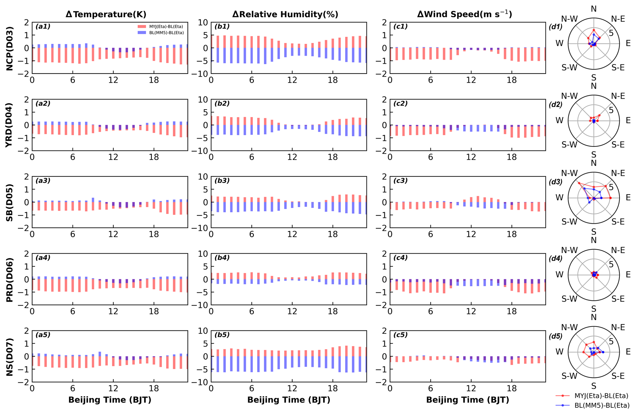
Figure 9Time series of diurnal variation in the effects of the PBL scheme and N-S schemes on (a1–a5) 2 m temperature, (b1–b5) 2 m relative humidity, (c1–c5) 10 m wind speed, and (d1–d5) 10 m wind direction for five regions in January.
It is not necessary to set the vertical resolution much finer compared to the horizontal resolution, and in this experiment 48 levels are fully sufficient to reproduce the vertical structure of the PBL.
3.3 Near-surface (N-S) scheme impact on PBL structures
For the impact of the N-S scheme, this section focuses on the changes in the N-S meteorological parameters. The N-S and PBL schemes are fixed pairings, and three experiments (i.e., Exp5, Exp6 and Exp7) are done by this study to distinguish the extent to which the N-S and PBL schemes affect the N-S meteorological parameters (2 m temperature, 2 m relative humidity, 10 m wind speed and direction). In terms of daily variation, the variation in temperature in the five regions is consistent, with similar simulated results in Exp5 (BL + MM5) and Exp7 (BL + Eta), and two experiments have notable differences from Exp6 (MYJ + Eta) (Fig. 8a1–a5). However, the relative humidity and temperature are different, and the results of Exp5 and Exp7 are not close to each other (Fig. 8b1–b5). From the results of wind speed, it is similar to the results of temperature, and the results of Exp5 and Exp7 are much closer, as is the wind direction (Fig. 8c1–d5). Furthermore, the three schemes are made differential to quantify the impact of the PBL scheme and N-S scheme. Exp6–Exp7 note the impact of the PBL scheme, and Exp5–Exp7 illustrate the effect of the N-S scheme.
As can be seen from Fig. 9a1–a5, the influence of the PBL scheme is greater compared to the N-S scheme in five regions. The difference in temperature simulated by different PBL schemes is about 1 K, while the difference for N-S schemes is just less than 0.5 K. In Fig. 9b1–b5, as in Fig. 8, the results for relative humidity differ from those for temperature. The PBL scheme and N-S scheme affect relative humidity to different degrees, with the PBL scheme having a smaller effect. Particularly in the NCP, SB, and NS regions, the impact of the PBL scheme is much smaller than that of the N-S scheme (Fig. 9b1, b3, b5). Regardless of the PBL scheme and N-S scheme, the effect is greater at night than during the day. The findings for wind speed and temperature are more similar, with the PBL scheme having a remarkably greater impact than the N-S scheme (Fig. 9c1–c5). Except for the daytime in both YRD and PRD regions, the N-S scheme has a slightly greater effect on wind speed than the PBL scheme (Fig. 9c2, c4). The wind direction is divided into a total of eight directions (N, NE, E, SE, S, SW, W, NW), and the influence of the PBL scheme is larger in terms of the the percentage frequency of each direction (Fig. 9d1–d5).
As for the regional distribution of temperatures, the distributions of Exp5 and Exp7 are more similar without regard to the region and differ considerably from that of Exp6 (Fig. 10). Therefore, for temperature, the effect of the PBL scheme is more important. For wind speed, Exp7 simulates the largest wind speed, followed by Exp5, and Exp6 has the smallest wind speed, noting that the PBL scheme has a larger degree of influence than the N-S scheme (Fig. 11).
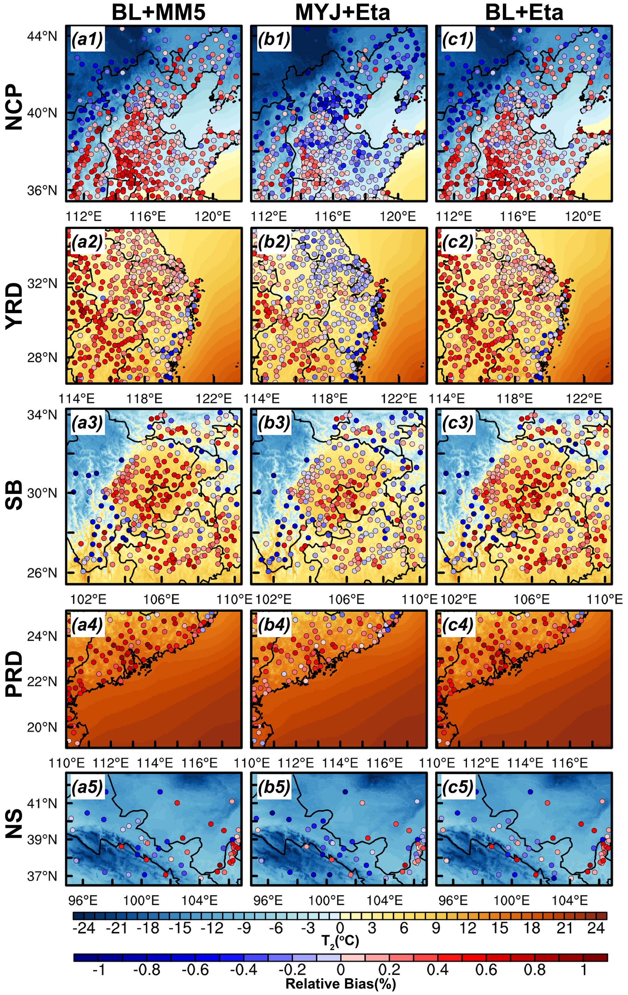
Figure 10Regional distribution of 2 m temperature simulated by the (a) BL + MM5, (b) MYJ + Eta, and (c) BL + Eta for five regions in January. The distribution of relative bias between the simulations and observations is denoted by scatters.
In general, for temperature, the choice of PBL scheme is of much more importance. For relative humidity, the PBL and N-S schemes are equally important, except for the NCP, SB, and NS regions, where the choice of the N-S scheme is more key. For wind speed and direction, the choice of PBL scheme is more critical, and the simulation of different PBL schemes leads to more differences in the results.
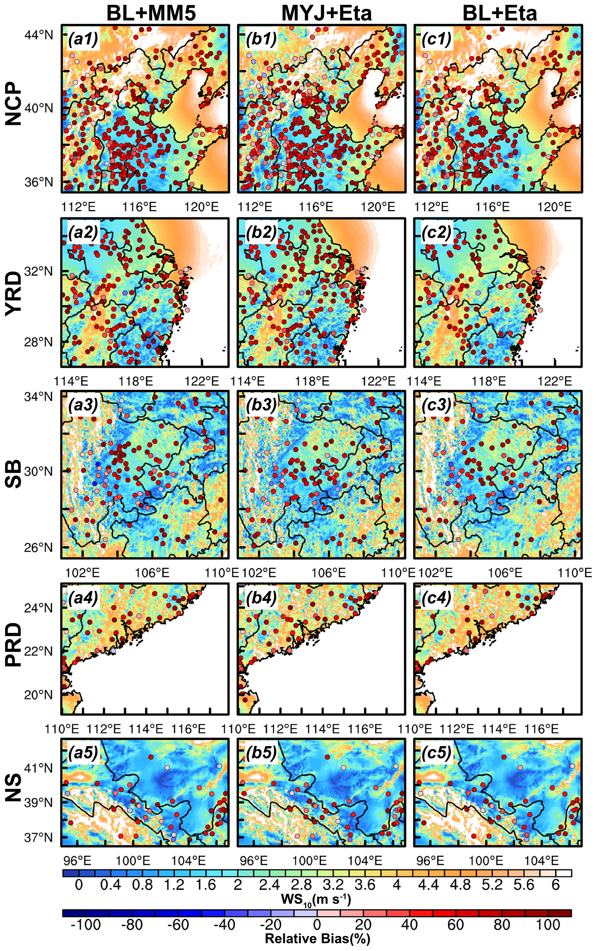
Figure 11Similar to Fig. 10 but for 10 m wind speed.
3.4 Effect of initial and boundary conditions on meteorological parameters
In this subsection, the same initial field and boundary conditions at different resolutions (i.e., FNL–1∘ and FNL–0.25∘) and different initial field and boundary conditions at the same resolution (i.e., FNL–0.25∘ and EC–0.25∘) are chosen to explore the effects of the initial field and boundary conditions on the meteorological field simulation. Figure 12 shows the daily variation series of 2 m temperature, 2 m relative humidity, and 10 m wind speed and direction. In addition, Fig. 12 notes that the effect of data with different resolutions of the same initial field on the results is small for temperature and relative humidity, but the effect of data with different initial fields of the same resolution is profound. For the five regions, the EC data better simulate the temperature than the FNL data during the day, while at night the difference between the two types of data simulating the temperature becomes less than during the day, except for the NCP and NS regions (where the temperature difference is larger for both day and night) (Fig. 12a1–a5). For relative humidity, the EC data are simulated better than the FNL data regardless of the region, playing a key role in improving the relative humidity results of the model (Fig. 12b1–b5). Overall, the increase in resolution of the initial field data from 1 to 0.25∘ has less effect on the simulation of temperature and relative humidity, while there is a striking difference between the different initial field data.
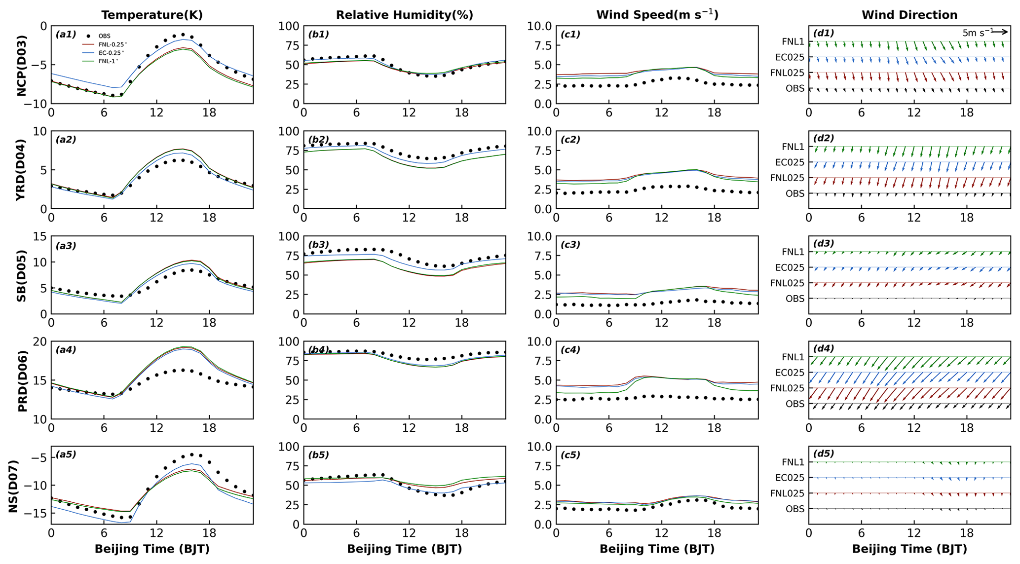
The results for wind speed differ from the first two parameters in that there is almost no difference between the three experiments for wind speed simulations during the day (Fig. 12c1–c5). However, different initial field data at the same resolution have very little effect on the wind speed, but the same initial field data at different resolutions have a significant effect on the wind speed, especially at night (Fig. 12c1–c5). All data have a negligible effect on the wind direction (Fig. 12d1–d5).
As mentioned earlier, the EC data have improved the results of relative humidity for all regions (Fig. 12b1–b5). In terms of regional distribution, the regional distribution of FNL data is similar in shape for different resolutions (Fig. 13a, c). However, the relative humidity distribution simulated by EC data and FNL data is drastically different (Fig. 13). It is worth noting that the relative humidity of the EC data is the highest in the four regions, with the exception of the NS region, where the relative humidity is the lowest (Fig. 13b1–b5).
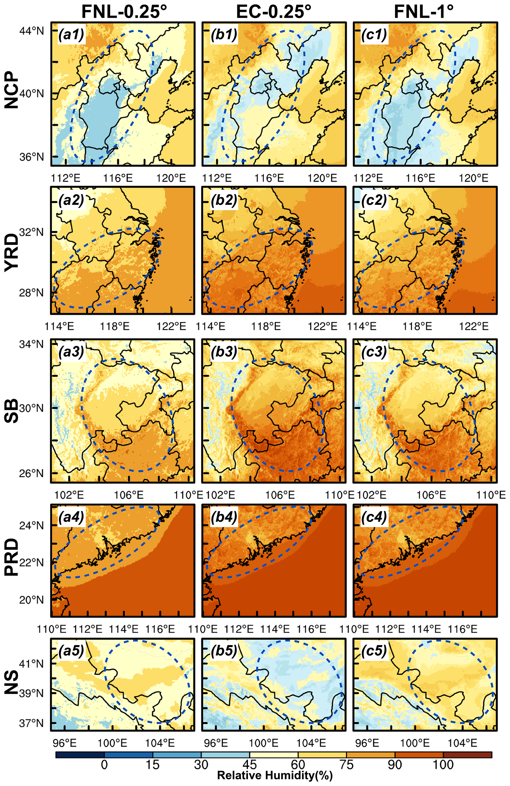
Figure 13Regional distribution of 2 m relative humidity simulated by the (a) FNL-0.25∘, (b) EC-0.25∘, and (c) FNL-1∘ for five regions in January. The dashed blue circles indicate the regions where the results of the three experimental simulations differ significantly.
In the vertical direction, the simulated results of the three experiments for temperature and wind speed do not differ much, unlike the near-surface meteorological parameters (i.e., T2, RH2, WS10, and WD10) that show such obvious differences (Figs. S1, S2 in the Supplement). Nevertheless, for the relative humidity, the variation in vertical direction at different heights is more consistent with the near-surface layer, where the relative humidity of EC data is high in the whole layer (Fig. S3). Except for a few highland stations outside the basin in the SB region, the relative humidity of EC data is low at higher altitudes (Fig. S3a3, b3, d3).
3.5 Effect of underlying surface on meteorological parameters
To further explore the impact of underlying surface changes on the simulation results of meteorological fields, we use the underlying surface data in January 2016 that are closer to the simulation time, in addition to the default underlying surface data that comes with the model, for comparative analysis of the simulation. Comparing Figs. 1 and 14, it can be concluded that the most substantial change in the domain 1 area is in the croplands type (i.e., code 12), especially for the area south of latitude 30∘ N. Many types with an underlying surface of 12 have become 14, 8, 9, etc. Although both 12 and 14 here can represent cropland, there are some differences in the specific descriptions. Code 12 mainly indicates that at least 60 % of area is cultivated cropland, while code 14 mainly refers to the mosaics of small-scale cultivation 40 %–60 % with natural tree, shrub, or herbaceous vegetation. In addition to croplands, the two types of urban and water bodies are more variable as well. Therefore, this subsection focuses on the effects of urban and water body changes on surface meteorological fields.
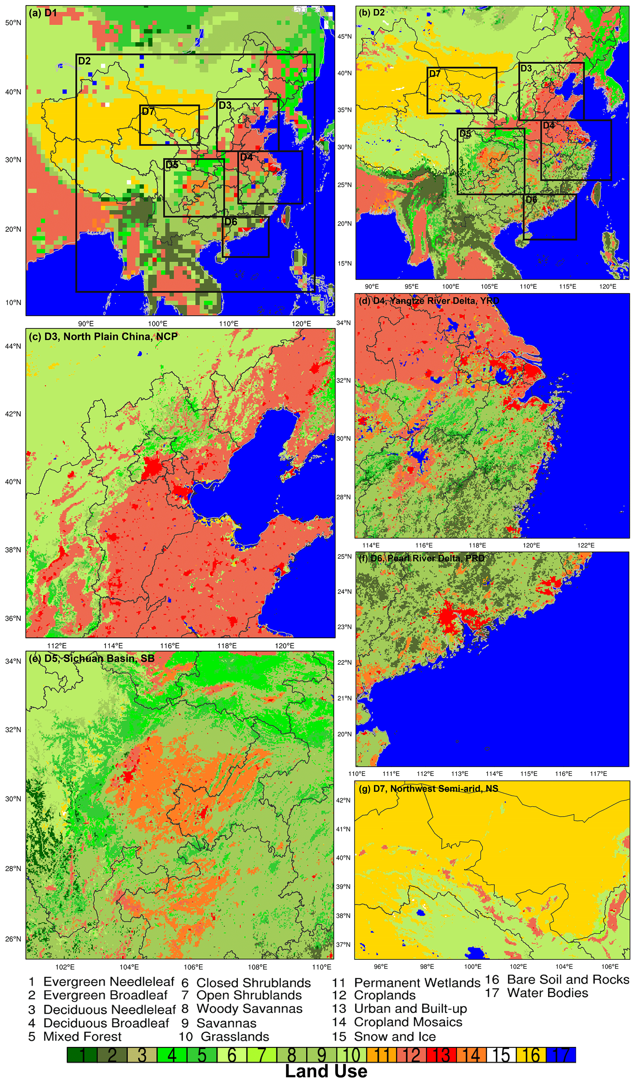
Figure 14Similar to Fig. 1 but for the land use type for January 2017.
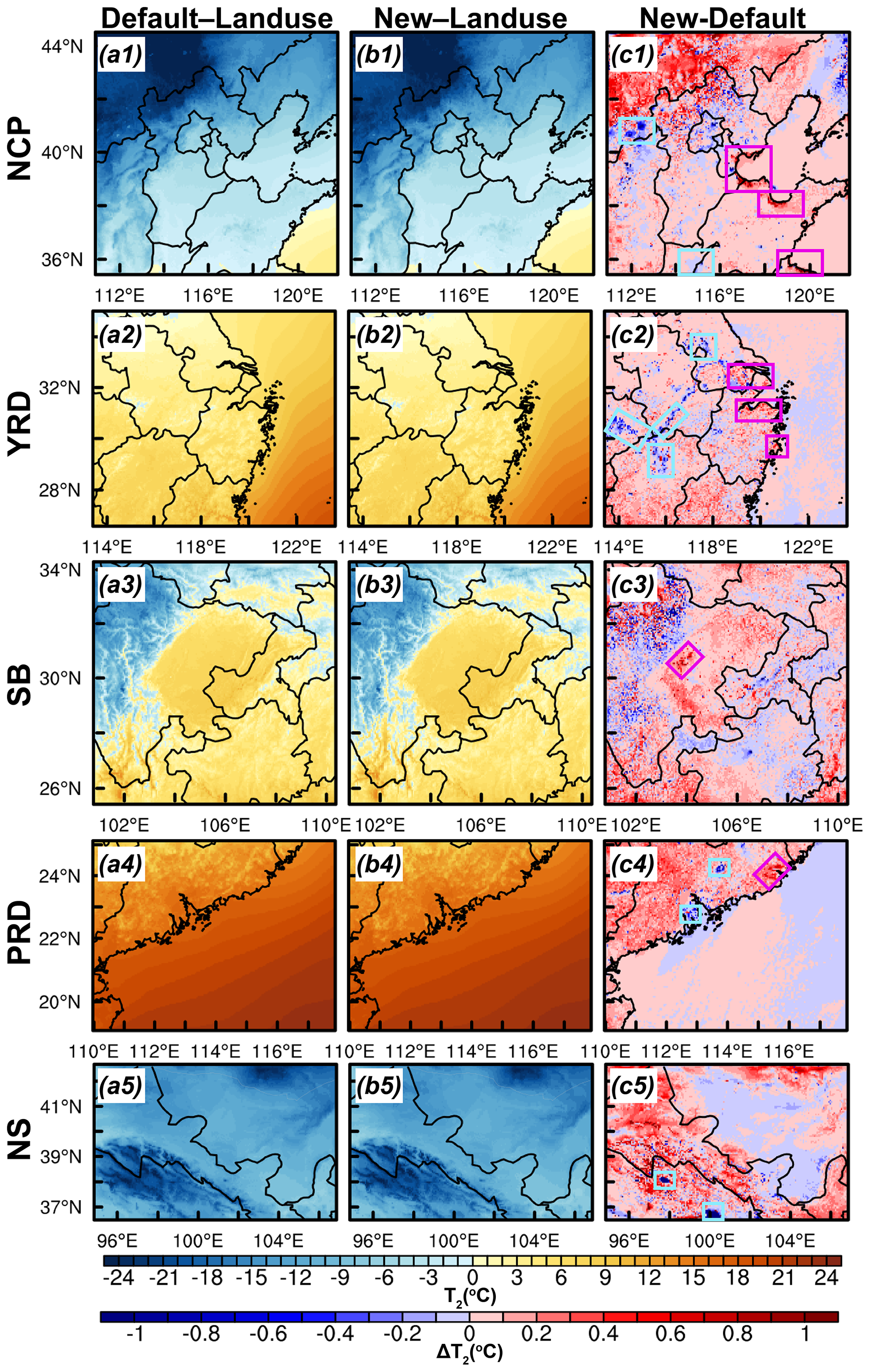
Figure 15Regional distribution of 2 m temperature simulated by the (a) default land use and (b) new land use and (c) the difference between the two land use types for five regions in January. The blue (red) box indicates the region where the wind speed decreases (increases) due to changes in the water bodies and urban areas.
In terms of the overall regional distribution, the new underlying surface did not affect the areas of high and low values of temperature (Fig. 15a–b) to an important degree. However, the difference between the simulation results of two different underlying surface shows that the change in the underlying surface has an effect on the temperature by about , especially for the grids with more obvious changes in water bodies and urban areas (Fig. 15c). In the NCP region, an increase in the area of water bodies in the coastal areas of Tianjin (TJ) municipality, Shandong (SD) province, and Jiangsu (JS) province leads to a distinct increase in temperature (i.e., indicated by red boxes), while a decrease in the area of inland water in the northern region of Shanxi (SX) province causes a decrease in temperature (i.e., denoted by blue boxes) (Fig. 15c1). The decrease in the area of water bodies in the Yangtze River in the YRD region has caused a decrease in temperature, while urbanization has contributed to an increase in temperature in several regions (Fig. 15c2). The underlying surface changes in the SB region are mainly in the form of forest and savanna changes, as well as the more rapid urbanization of the provincial capital city of Chengdu (CD) municipality (Fig. 14e). The development of this city has a positive feedback effect on the temperature of the region (Fig. 15c3). The underlying surface change in the YRD region is from croplands to savannas, with a rapid greening rate, and its excessive greening may make the green coverage of some cities too high, leading some grids to identify the cities as savannas. In the NS region, the area of croplands and cities along the Qilian Mountains increases, while the area of some inland lakes decreases, in turn leaving some influence on the results of the temperature.
The wind field does not vary as regularly as the temperature filed. Except for the variation in water body area which has a more consistent pattern on the wind field, all other types of underlying surface variation have a haphazard effect on the wind field (Fig. S4).
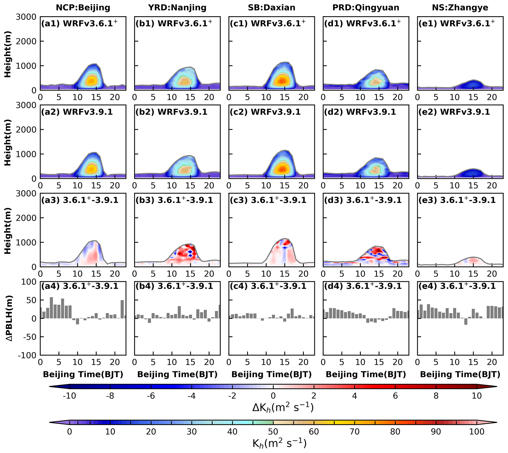
Figure 16Time–height cross sections of heat turbulent diffusion coefficient (TDC) simulated by (a1–e1) WRFv3.6.1+ and (a2–e2) WRFv3.9.1 and (a3–e3) the difference between the TDC of the two versions. (a4–e4) Time series of diurnal variation in the difference between the PBLH of the two versions. The gray line in (a1)–(e3) indicates the PBLH.
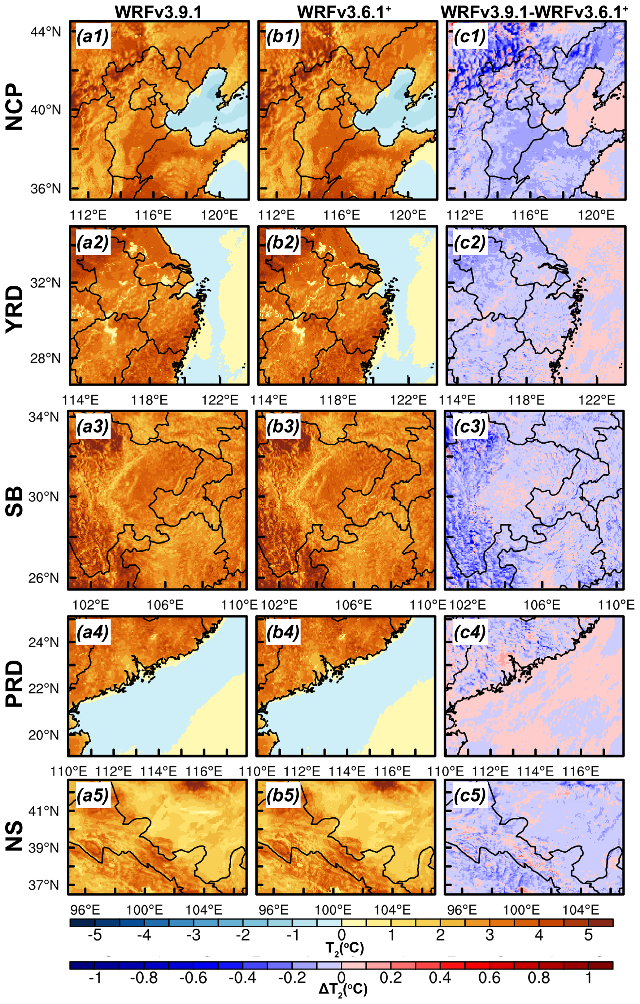
Figure 17Regional distribution of diurnal 2 m temperature range simulated by the (a) WRFv3.9.1 and (b) WRFv3.6.1+ and (c) the difference between the two versions for five regions in January.
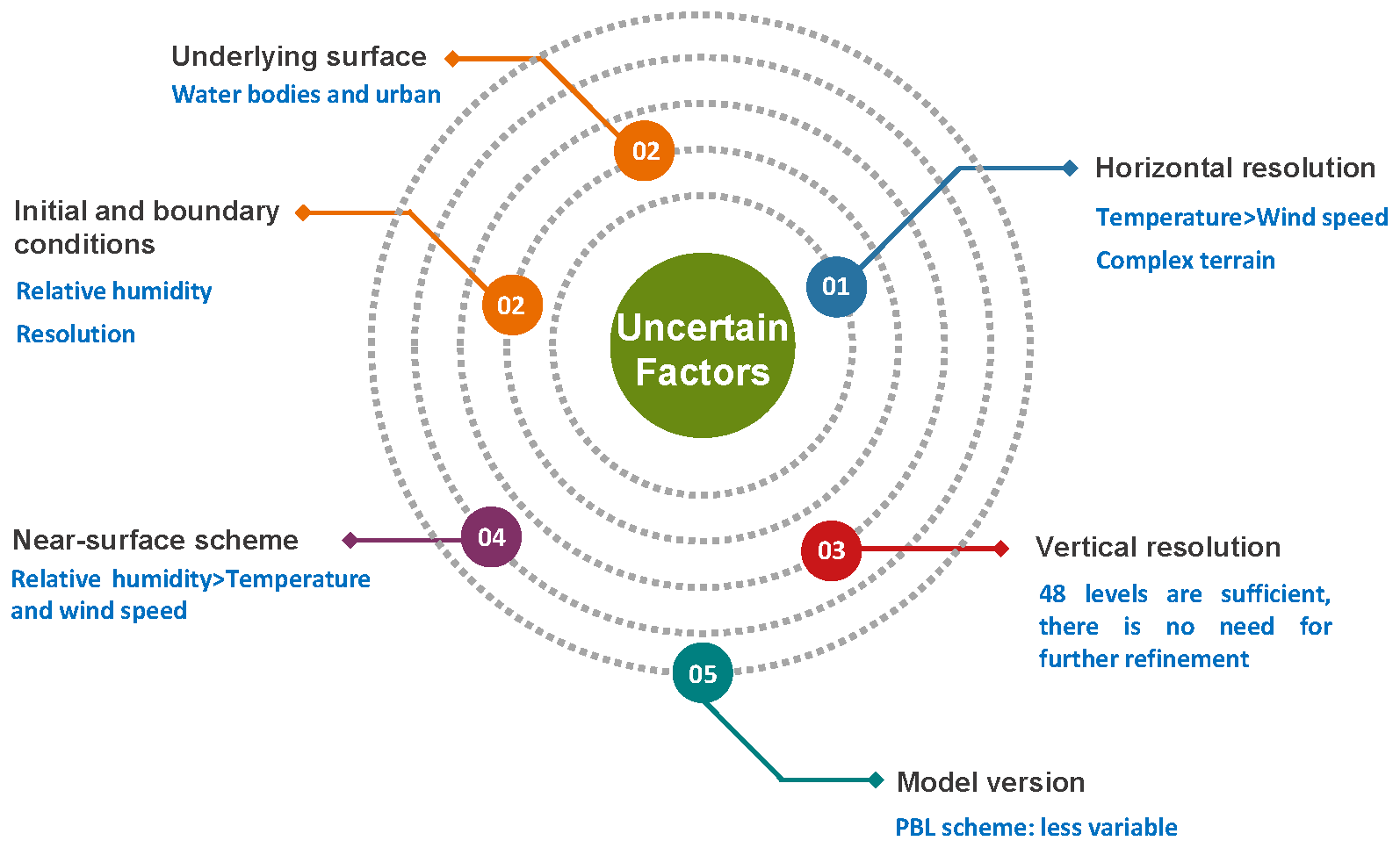
Figure 18An overview figure of the prioritization of uncertainties, where the uncertainties are in black font and the elements focused on in that factor are in blue font.
3.6 Impact of the model version update
As computer technology continues to evolve, the parameterizations in the model are being upgraded and improved, but it is worthwhile further exploring how much the parameterizations and versions affect the simulation results of the model. For the PBL parameterization scheme, turbulent diffusion is crucial for the vertical mixing of momentum, heat, water vapor, and pollutants within the PBL. In December 2014, the ACM2 parameterization scheme received two major updates. (1) The turbulent diffusion coefficients of heat were updated, meaning that the stability function of Richardson number was modified; this is expected to reduce the day and night 2 m temperature bias. (2) The bug that the minimum value of the planetary boundary layer height (PBLH) is lower than the height of the first level of the model under stable conditions has been repaired, and the minimum value of the PBLH is fixed to the height of the first level of the model. We therefore choose the ACM2 scheme in WRFv3.6.1 as a control experiment. In the control experiment, the ACM2 scheme in the WRFv3.9.1 version is replaced with WRFv3.6.1, and all other schemes are kept in WRFv3.9.1 (i.e., WRFv3.6.1+). This ensures that the difference between the two experiments is the representative of the impact of the ACM2 scheme update.
The difference between the turbulent diffusion coefficient of heat calculated by the two versions lies in the different principles of calculation using the Richardson number (Ri) method. In WRFv3.6.1+, Ri is used to judge the stability, while is also used to additionally constrain the stability and determine the empirical stability function. In contrast, only Ri is adopted to determine the function in WRFv3.9.1. Figure 16 shows the diurnal variation in turbulent diffusion coefficient of heat with height, as well as the difference with PBLH. In general, the two versions have no effect on the overall trend of turbulent diffusion coefficient (TDC) (Fig. 16a1–e2). However, within the PBL, the TDC of WRFv3.9.1 is smaller than that of WRFv3.6.1+, with the most significant difference during the daytime. Meanwhile, in some regions at night, a TDC of WRFv3.9.1 is also greater than that of WRFv3.6.1+ (Fig. 16a3–e3). In addition, the differences among the five regions slightly vary. The deviation in the NCP, SB, and NS regions is small, around 2 m2 s−1 (Fig. 16a3, c3, e3), while the deviation in the YRD and PRD regions is large, up to about 10 m2 s−1 (Fig. 16b3, d3). The TDC modification aims to reduce the temperature difference between day and night. Indeed, this expectation is fulfilled. It can be noticed in Fig. 17 that the diurnal temperature difference for WRFv3.9.1 is smaller than that of WRFv3.6.1+ in almost all regions (except for the area where the underlying surface is water). In addition, we need to pay attention to the variation in the PBLH. As shown in Fig. 16, the difference in PBLH during daytime is smaller than at night, and the PBLH of WRFv3.9.1 is lower than that of WRFv3.6.1+. The model WRFv3.9.1 fixes the minimum value of the PBLH to the first level height, markedly reducing the PBLH at night. However, this approach may be too crude and parsimonious to cause problems and should be corrected in the future.
The simulation results of the model within the PBL are subject to many factors, but its portrayal and description by the PBL parameterization schemes plays a vital role in affecting the variation in the meteorological field. The simulations of the PBL schemes on the meteorological fields were described in Part 1. In Part 2, further uncertainties affecting the results of the meteorological field have been evaluated and analyzed, and the degree of influence of different factors has been compared, in the hope of providing a reference for scholars conducting research on the model. In addition to the dominant role of the PBL scheme on the results of the meteorological field, many elements in the model are influenced by large uncertainties. For example, what is the effect of horizontal resolution, and how much does the result vary under different resolution conditions? Is the continuous encryption of the vertical levels necessary for the simulation of the vertical structure of the PBL? Which has a greater impact on the results of the meteorological field, the near-surface (N-S) layer scheme or the PBL scheme? What is the impact of these changes on the underlying surface, which is constantly updated by the development of urbanization? The innovation of computer technology has provided the opportunity to keep the model updated. How much effect will the updates have on different versions of the model results? The simulation of the model depends on the initial and boundary conditions, so how much do the initial and boundary conditions of different resolutions and products affect the model results? These uncertainties have not been fully evaluated and analyzed yet. To resolve the confusions, this study synthesizes the effects of the above factors on the model results.
- a.
Effect of the horizontal resolution. The three different resolutions have a more dramatic effect on temperature than on wind speed (Fig. 18). Regardless of the region, the distribution of temperature deviations simulated at 75 km resolution is clearly different from that of 15 and 3 km, especially in areas with more complex topography, such as the NCP, SB, and NS regions. All three resolutions overestimate the wind speed in all regions, except for the 75 km resolution, where there is an underestimation of the wind speed at the stations around the basin in the SB region (Fig. 18). The difference between the resolutions decreases with increasing temperature but becomes more pronounced with increasing wind speed.
- b.
Effect of the vertical resolution. The number of vertical levels of the model is encrypted from 48 to 62 levels with almost no effect on the vertical structure of the PBL. Meanwhile, the increase in the number of vertical levels brings an increase in memory of about 150 GB for one month. Compared to the horizontal resolution, the vertical resolution does not need to be set particularly fine, and 48 levels are perfectly sufficient to reproduce the evolution of the PBL structure (Fig. 18).
- c.
Influence of the N-S scheme. The PBL scheme makes a greater impact on the simulated results for temperature, wind speed, and direction, while for relative humidity, the N-S scheme contributes greatly, especially in the NCP, SB, and NS regions. For either scheme, the effect is much greater at night than during the daytime. In general, the choice of the PBL scheme is more critical for temperature and wind fields, but for relative humidity the PBL and N-S schemes are equally important (Fig. 18).
- d.
Impact of the initial and boundary conditions. The effect of data of different resolutions of the same product on the results of temperature and relative humidity is small, but the influence of data of different products of the same resolution is large. EC data simulates temperature better than FNL data during the daytime, while at night the difference between the two datasets is relatively small (except for the NCP and NS regions). The EC data simulate the relative humidity better than the FNL data regardless of the region, even in the vertical direction, which will expose a key way to improve the relative humidity results of the model in the future (Fig. 18). Nonetheless, data of the same resolution but different products exhibit no obvious effect on wind speed, while the influence of data from the same product with different resolutions is larger, especially at night.
- e.
Effect of the underlying surface. In terms of regional distribution, the new underlying surface make no significant difference with respect to the temperature. However, for the grids with more pronounced changes in water bodies and urban areas, the change in underlying surface has an approximate influence on temperature (Fig. 18). An increase (decrease) in the area of water bodies leads to an increase (decrease) in temperature, and the growth of urbanization brings about an increase in temperature. The variation in the wind field is not as regular as temperature. Except for the changes in the area of water bodies that affect the wind field consistently, other types of underlying surface changes show a haphazard effect on the wind filed.
- f.
Influence of the model version. The update of the PBL scheme reduces the day and night 2 m temperature bias. However, the simple definition method of fixing the minimum value of the PBLH as the first level height of the model may have some defects. The change in the stability function of the Richardson number alters the turbulent diffusion coefficient of heat, which is more distinct in the daytime, with a deviation of about 10 m2 s−1. The PBL parameterization scheme in the current model is less modified (Fig. 18).
In summary, the horizontal resolution is more influential than the vertical resolution. The N-S scheme has less effect than the PBL scheme on the results of temperature and wind speed. In addition, the initial and boundary conditions of different products have the most significant influence on relative humidity. Grid changes where the underlying surface is urban and water bodies have a more pronounced effect on the results of meteorological fields, especially for temperature. The PBL parameterization schemes in versions WRFv3.9.1 and WRFv3.6.1 have changed less and have less impact on the simulation of model results (Fig. 18). A piece of advice we can give is that the needs of different scholars for the model vary a lot, meaning that the configuration of uncertainties requires a comprehensive consideration to obtain the optimal results for the analysis.
The source codes of WRF versions 3.9.1 and 3.6.1 can be found on the following website: https://www2.mmm.ucar.edu/wrf/users/download/ (Skamarock et al., 2008). The original model settings file is already included in Supplement to Part 1, while the other model settings file used in Part 2 is provided under the filename “L62_namelist.input” and is already included in Supplement. In addition, the observations used are also provided in Supplement to Part 1. The initial field and boundary condition data and the underlying surface data are provided in the text.
The supplement related to this article is available online at: https://doi.org/10.5194/gmd-16-6833-2023-supplement.
Development of the ideas and concepts behind this work was performed by all the authors. Model execution, data analysis, and paper preparation were performed by WJ. XZ and HW provided computing resources and offered advice and feedback. YW, DW, and JZ supported the data. WZ, LZ, LG, YL, JW, YY, and YL provided suggestions. All authors contributed to the manuscript.
The contact author has declared that none of the authors has any competing interests.
Publisher's note: Copernicus Publications remains neutral with regard to jurisdictional claims made in the text, published maps, institutional affiliations, or any other geographical representation in this paper. While Copernicus Publications makes every effort to include appropriate place names, the final responsibility lies with the authors.
The work was carried out at the National Supercomputer Center in Tianjin, and the calculations were performed on TianHe-1 (A).
This research has been supported by the National Natural Science Foundation of China (NSFC) Major Project (42090031), NSFC Project (U19A2044), and the Basic Research Fund of the Chinese Academy of Meteorological Sciences (CAMS) (2023Y003).
This paper was edited by Chiel van Heerwaarden and reviewed by two anonymous referees.
Bhati, S. and Mohan, M.: WRF model evaluation for the urban heat island assessment under varying land use/land cover and reference site conditions, Theor. Appl. Climatol., 126, 385–400, https://doi.org/10.1007/s00704-015-1589-5, 2016.
Chang, P., Zhang, S., Danabasoglu, G., Yeager, S. G., Fu, H., Wang, H., Castruccio, F. S., Chen, Y., Edwards, J., Fu, D., Jia, Y., Laurindo, L. C., Liu, X., Rosenbloom, N., Small, R. J., Xu, G., Zeng, Y., Zhang, Q., Bacmeister, J., Bailey, D. A., Duan, X., DuVivier, A. K., Li, D., Li, Y., Neale, R., Stössel, A., Wang, L., Zhuang, Y., Baker, A., Bates, S., Dennis, J., Diao, X., Gan, B., Gopal, A., Jia, D., Jing, Z., Ma, X., Saravanan, R., Strand, W. G., Tao, J., Yang, H., Wang, X., Wei, Z., and Wu, L.: An Unprecedented Set of High-Resolution Earth System Simulations for Understanding Multiscale Interactions in Climate Variability and Change, J. Adv. Model. Earth Sy., 12, e2020MS002298, https://doi.org/10.1029/2020MS002298, 2020.
Friedl, M. A., McIver, D. K., Hodges, J. C. F., Zhang, X. Y., Muchoney, D., Strahler, A. H., Woodcock, C. E., Gopal, S., Schneider, A., Cooper, A., Baccini, A., Gao, F., and Schaaf, C.: Global land cover mapping from MODIS: algorithms and early results, Remote Sens. Environ., 83, 287–302, https://doi.org/10.1016/S0034-4257(02)00078-0, 2002.
García-García, A., Cuesta-Valero, F. J., Beltrami, H., González-Rouco, J. F., and García-Bustamante, E.: WRF v.3.9 sensitivity to land surface model and horizontal resolution changes over North America, Geosci. Model Dev., 15, 413–428, https://doi.org/10.5194/gmd-15-413-2022, 2022.
Jia, W. and Zhang, X.: The role of the planetary boundary layer parameterization schemes on the meteorological and aerosol pollution simulations: A review, Atmos. Res., 239, 104890, https://doi.org/10.1016/j.atmosres.2020.104890, 2020.
Jia, W., Zhang, X., Wang, H., Wang, Y., Wang, D., Zhong, J., Zhang, W., Zhang, L., Guo, L., Lei, Y., Wang, J., Yang, Y., and Lin, Y.: Comprehensive evaluation of typical planetary boundary layer (PBL) parameterization schemes in China – Part 1: Understanding expressiveness of schemes for different regions from the mechanism perspective, Geosci. Model Dev., 16, 6635–6670, https://doi.org/10.5194/gmd-16-6635-2023, 2023.
Li, D., Chang, P., Yeager, S. G., Danabasoglu, G., Castruccio, F. S., Small, J., Wang, H., Zhang, Q., and Gopal, A.: The Impact of Horizontal Resolution on Projected Sea-Level Rise Along US East Continental Shelf With the Community Earth System Model, J. Adv. Model. Earth Sy., 14, e2021MS002868, https://doi.org/10.1029/2021MS002868, 2022.
Li, J., Bao, Q., Liu, Y., Wang, L., Yang, J., Wu, G., Wu, X., He, B., Wang, X., Zhang, X., Yang, Y., and Shen, Z.: Effect of horizontal resolution on the simulation of tropical cyclones in the Chinese Academy of Sciences FGOALS-f3 climate system model, Geosci. Model Dev., 14, 6113–6133, https://doi.org/10.5194/gmd-14-6113-2021, 2021.
Li, Y., Gao, Z., Lenschow, D. H., and Chen, F.: An Improved Approach for Parameterizing Surface-Layer Turbulent Transfer Coefficients in Numerical Models, Bound.-Lay. Meteorol., 137, 153–165, https://doi.org/10.1007/s10546-010-9523-y, 2010.
Ma, Z., Liu, Q., Zhao, C., Shen, X., Wang, Y., Jiang, J. H., Li, Z., and Yung, Y.: Application and Evaluation of an Explicit Prognostic Cloud-Cover Scheme in GRAPES Global Forecast System, J. Adv. Model. Earth Sy., 10, 652–667, https://doi.org/10.1002/2017MS001234, 2018.
Ma, Z., Zhao, C., Gong, J., Zhang, J., Li, Z., Sun, J., Liu, Y., Chen, J., and Jiang, Q.: Spin-up characteristics with three types of initial fields and the restart effects on forecast accuracy in the GRAPES global forecast system, Geosci. Model Dev., 14, 205–221, https://doi.org/10.5194/gmd-14-205-2021, 2021.
Magnusson, L. and Källén, E.: Factors Influencing Skill Improvements in the ECMWF Forecasting System, Mon. Weather Rev., 141, 3142–3153, https://doi.org/10.1175/mwr-d-12-00318.1, 2013.
Menut, L., Bessagnet, B., Colette, A., and Khvorostiyanov, D.: On the impact of the vertical resolution on chemistry-transport modelling, Atmos. Environ., 67, 370–384, https://doi.org/10.1016/j.atmosenv.2012.11.026, 2013.
Morichetti, M., Madronich, S., Passerini, G., Rizza, U., Mancinelli, E., Virgili, S., and Barth, M.: Comparison and evaluation of updates to WRF-Chem (v3.9) biogenic emissions using MEGAN, Geosci. Model Dev., 15, 6311–6339, https://doi.org/10.5194/gmd-15-6311-2022, 2022.
National Centers for Environmental Prediction/National Weather Service/NOAA/U.S. Department of Commerce: NCEP FNL Operational Model Global Tropospheric Analyses, continuing from July 1999, Research Data Archive at the National Center for Atmospheric Research, Computational and Information Systems Laboratory, https://doi.org/10.5065/D6M043C6, 2000 (updated daily).
National Centers for Environmental Prediction/National Weather Service/NOAA/U.S. Department of Commerce: NCEP GDAS/FNL 0.25 Degree Global Tropospheric Analyses and Forecast Grids, Research Data Archive at the National Center for Atmospheric Research, Computational and Information Systems Laboratory, https://doi.org/10.5065/D65Q4T4Z, 2015 (updated daily).
Nolan, D. S. and Onderlinde, M. J.: The Representation of Spiral Gravity Waves in a Mesoscale Model With Increasing Horizontal and Vertical Resolution, J. Adv. Model. Earth Sy., 14, e2022MS002989, https://doi.org/10.1029/2022MS002989, 2022.
O'Dea, E., Furner, R., Wakelin, S., Siddorn, J., While, J., Sykes, P., King, R., Holt, J., and Hewitt, H.: The CO5 configuration of the 7 km Atlantic Margin Model: large-scale biases and sensitivity to forcing, physics options and vertical resolution, Geosci. Model Dev., 10, 2947–2969, https://doi.org/10.5194/gmd-10-2947-2017, 2017.
Ouyang, Z., Sciusco, P., Jiao, T., Feron, S., Lei, C., Li, F., John, R., Fan, P., Li, X., Williams, C. A., Chen, G., Wang, C., and Chen, J.: Albedo changes caused by future urbanization contribute to global warming, Nat. Commun., 13, 3800, https://doi.org/10.1038/s41467-022-31558-z, 2022.
Qian, Y., Chakraborty, T. C., Li, J., Li, D., He, C., Sarangi, C., Chen, F., Yang, X., and Leung, L. R.: Urbanization Impact on Regional Climate and Extreme Weather: Current Understanding, Uncertainties, and Future Research Directions, Adv. Atmos. Sci., 39, 819–860, https://doi.org/10.1007/s00376-021-1371-9, 2022.
Roberts, M. J., Jackson, L. C., Roberts, C. D., Meccia, V., Docquier, D., Koenigk, T., Ortega, P., Moreno-Chamarro, E., Bellucci, A., Coward, A., Drijfhout, S., Exarchou, E., Gutjahr, O., Hewitt, H., Iovino, D., Lohmann, K., Putrasahan, D., Schiemann, R., Seddon, J., Terray, L., Xu, X., Zhang, Q., Chang, P., Yeager, S. G., Castruccio, F. S., Zhang, S., and Wu, L.: Sensitivity of the Atlantic Meridional Overturning Circulation to Model Resolution in CMIP6 HighResMIP Simulations and Implications for Future Changes, J. Adv. Model. Earth Sy., 12, e2019MS002014, https://doi.org/10.1029/2019MS002014, 2020.
Rummukainen, M.: Added value in regional climate modeling, WIREs Climate Change, 7, 145–159, https://doi.org/10.1002/wcc.378, 2016.
Schwaab, J., Meier, R., Mussetti, G., Seneviratne, S., Bürgi, C., and Davin, E. L.: The role of urban trees in reducing land surface temperatures in European cities, Nat. Commun., 12, 6763, https://doi.org/10.1038/s41467-021-26768-w, 2021.
Singh, J., Singh, N., Ojha, N., Sharma, A., Pozzer, A., Kiran Kumar, N., Rajeev, K., Gunthe, S. S., and Kotamarthi, V. R.: Effects of spatial resolution on WRF v3.8.1 simulated meteorology over the central Himalaya, Geosci. Model Dev., 14, 1427–1443, https://doi.org/10.5194/gmd-14-1427-2021, 2021.
Skamarock, W. C., Klemp, J. B., Dudhia, J., Gill, D. O., Barker, D., Duda, M. G., and Powers, J. G.: A Description of the Advanced Research WRF Version 3 (No. NCAR/TN475+STR), University Corporation for Atmospheric Research, https://doi.org/10.5065/D68S4MVH, 2008 (data available at: https://www2.mmm.ucar.edu/wrf/users/download/ last access: 22 November 2023).
Small, R. J., Bacmeister, J., Bailey, D., Baker, A., Bishop, S., Bryan, F., Caron, J., Dennis, J., Gent, P., Hsu, H.-M., Jochum, M., Lawrence, D., Muñoz, E., diNezio, P., Scheitlin, T., Tomas, R., Tribbia, J., Tseng, Y.-H., and Vertenstein, M.: A new synoptic scale resolving global climate simulation using the Community Earth System Model, J. Adv. Model. Earth Sy., 6, 1065–1094, https://doi.org/10.1002/2014MS000363, 2014.
Taylor, K. E., Stouffer, R. J., and Meehl, G. A.: An Overview of CMIP5 and the Experiment Design, B. Am. Meteor. Soc., 93, 485–498, https://doi.org/10.1175/bams-d-11-00094.1, 2012.
Teixeira, J. C., Carvalho, A. C., Tuccella, P., Curci, G., and Rocha, A.: WRF-chem sensitivity to vertical resolution during a saharan dust event, Phys. Chem. Earth, 94, 188–195, https://doi.org/10.1016/j.pce.2015.04.002, 2016.
Tolentino, J., Rejuso, M. V., Inocencio, L. C., Ang, M. R. C., and Bagtasa, G.: Effect of horizontal and vertical resolution for wind resource assessment in Metro Manila, Philippines using Weather Research and Forecasting (WRF) model, Vol. 10005, SPIE, https://doi.org/10.1117/12.2241952, 2016.
Wang, L. and Li, D.: Urban Heat Islands during Heat Waves: A Comparative Study between Boston and Phoenix, J. Appl. Meteorol. Clim., 60, 621–641, https://doi.org/10.1175/JAMC-D-20-0132.1, 2021.
Weigel, A. P., Chow, F. K., and Rotach, M. W.: The effect of mountainous topography on moisture exchange between the “surface” and the free atmosphere, Bound.-Lay. Meteorol., 125, 227–244, https://doi.org/10.1007/s10546-006-9120-2, 2007.
Zhou, B., Zhu, K., and Xue, M.: A Physically Based Horizontal Subgrid-Scale Turbulent Mixing Parameterization for the Convective Boundary Layer, J. Atmos.Sci., 74, 2657–2674, https://doi.org/10.1175/jas-d-16-0324.1, 2017.