the Creative Commons Attribution 4.0 License.
the Creative Commons Attribution 4.0 License.
 | 15 Nov 2023
Evaluating 3 decades of precipitation in the Upper Colorado River basin from a high-resolution regional climate model
William Rudisill
Alejandro Flores
Rosemary Carroll
Convection-permitting regional climate models (RCMs) have recently become tractable for applications at multi-decadal timescales. These types of models have tremendous utility for water resource studies, but better characterization of precipitation biases is needed, particularly for water-resource-critical mountain regions, where precipitation is highly variable in space, observations are sparse, and the societal water need is great. This study examines 34 years (1987–2020) of RCM precipitation from the Weather Research and Forecasting model (WRF; v3.8.1), using the Climate Forecast System Reanalysis (CFS; CFSv2) initial and lateral boundary conditions and a 1 km × 1 km innermost grid spacing. The RCM is centered over the Upper Colorado River basin, with a focus on the high-elevation, 750 km2 East River watershed (ERW), where a variety of high-impact scientific activities are currently ongoing. Precipitation is compared against point observations (Natural Resources Conservation Service Snow Telemetry or SNOTEL), gridded climate datasets (Newman, Livneh, and PRISM), and Bayesian reconstructions of watershed mean precipitation conditioned on streamflow and high-resolution snow remote-sensing products. We find that the cool-season precipitation percent error between WRF and 23 SNOTEL gauges has a low overall bias ( = 0.25 %, s = 13.63 %) and that WRF has a higher percent error during the warm season ( = 10.37 %, s = 12.79 %). Warm-season bias manifests as a high number of low-precipitation days, though the low-resolution or SNOTEL gauges limit some of the conclusions that can be drawn. Regional comparisons between WRF precipitation accumulation and three different gridded datasets show differences on the order of ± 20 %, particularly at the highest elevations and in keeping with findings from other studies. We find that WRF agrees slightly better with the Bayesian reconstruction of precipitation in the ERW compared to the gridded precipitation datasets, particularly when changing SNOTEL densities are taken into account. The conclusions are that the RCM reasonably captures orographic precipitation in this region and demonstrates that leveraging additional hydrologic information (streamflow and snow remote-sensing data) improves the ability to characterize biases in RCM precipitation fields. Error characteristics reported in this study are essential for leveraging the RCM model outputs for studies of past and future climates and water resource applications. The methods developed in this study can be applied to other watersheds and model configurations. Hourly 1 km × 1 km precipitation and other meteorological outputs from this dataset are publicly available and suitable for a wide variety of applications.
- Article
(10057 KB) - Full-text XML
-
Supplement
(590 KB) - BibTeX
- EndNote


The last decade has demonstrated that non-hydrostatic, convection-permitting regional climate models (RCMs) are tools capable of simulating precipitation in complex mountain terrain (Ikeda et al., 2010; Rasmussen et al., 2011; Gutmann et al., 2012; Liu et al., 2017) and performing the related task of modeling mountain snow accumulations (Currier et al., 2017; Wrzesien et al., 2019), of which precipitation is the first-order control. Over 1.6 billion people directly rely on water resources flowing from mountain regions (Immerzeel et al., 2020), often in the form of seasonal snowpacks. At the same time, mountains are uniquely sensitive to climate change (Mountain Research Initiative Edw Working Group et al., 2015), and snowpacks are forecast to decline significantly in the coming decades (Siirila-Woodburn et al., 2021).
However, evaluating biases in precipitation from regional models is a persistent challenge, as gridded, gauge-based datasets that are commonly considered to be a gold standard can disagree substantially in mountain watersheds because of methodological choices alone and should themselves be considered to be model products and not treated wholly as observations (Henn et al., 2018; Lundquist et al., 2019). Gridded gauge-based precipitation datasets use various strategies to map sparse gauge observations across the terrain using topographic-based regressions (Daly et al., 2008; Thornton et al., 2016). Remote-sensing-based precipitation products (Ashouri et al., 2015) are not as suitable for stratiform clouds or those composed of ice-phase hydrometeors, which are both common cases for precipitation in the mountains of the western United States (Lettenmaier et al., 2015). Ground-based radar systems can measure precipitation rates (Lin and Mitchell, 2005), but radar beam blockage limits the utility in complex terrain (Maddox et al., 2002). It is fair to say that more work needs to be done to interrogate precipitation budgets in mountain watersheds, from RCMs or otherwise, as completely adequate observation data are not available at sufficient scales. Lundquist et al. (2019) articulate this point well and urge the community to consider the syntheses of indirect hydrologic information such as, but not limited to, ecological indicators, soil moisture, snowpack, and streamflow in order to better constrain precipitation inputs into mountainous watersheds. The uncertainties in precipitation data (rates, phases, and magnitudes) propagate into studies of hydrologic systems for water resource applications, snow modeling applications (Raleigh et al., 2015), and aqueous biogeochemistry (Maina et al., 2020), so improving the quality of precipitation data is of critical importance in a variety of sectors.
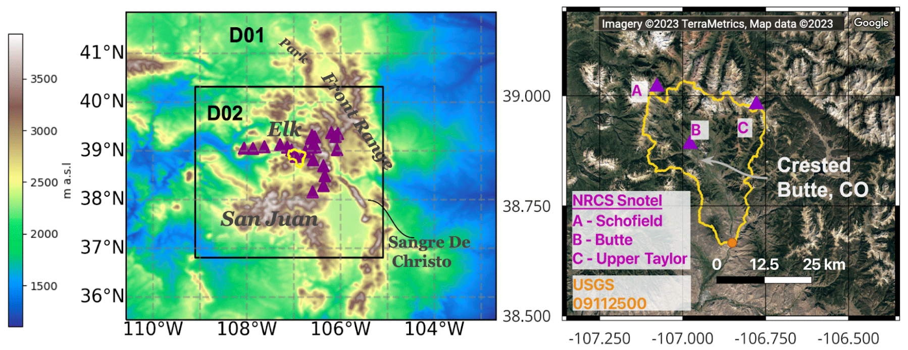
Figure 1WRF model domains and East River watershed (ERW), with the elevation (left) and satellite imagery (right) displayed. The outer nest (D01) is 3 km , and the inner domain (D02) is 1 km . Purple triangles show the locations of the SNOTEL sites examined in this study, and the orange circle shows the USGS stream gauge at the outlet of the ERW. Major mountain ranges are also labeled.
To meet this challenge, this study evaluates 34 years of Weather Research and Forecasting model version 3.8.1 (WRF v3.8.1)-simulated precipitation for a domain encompassing the Upper Colorado River basin. Special emphasis is placed on the East River watershed (ERW), a high-elevation ∼ 750 km2 watershed in the domain's center, where a variety of hydrologic and atmospheric field campaigns are being conducted. The ERW (Fig. 1) is an exemplar of Rocky Mountain landscapes (Hubbard et al., 2018) and flows from the Elk Mountains, approximately in the center of the WRF model domain described in the next section. The elevation ranges between 2500 and 4200 m above sea level. Subsets of the WRF data from this study have been made available publicly (Rudisill et al., 2022) to provide a baseline of high-resolution climate conditions for scientific activities taking place in the ERW, which include the U.S. Department of Energy East River Watershed Function Science Focus Area (Hubbard et al., 2018), Surface Atmosphere Integrated Field Laboratory (SAIL) campaign (Feldman et al., 2021), and the NOAA Study of Precipitation, the Lower Atmosphere and Surface for Hydrometeorology (SPLASH) field campaign (https://psl.noaa.gov/splash/, last access: 31 October 2023; de Boer et al., 2023). The Upper Colorado River basin is currently undergoing a devastating multi-year drought, and this study is timely in so far that it seeks to provide insight into the quantification of precipitation during the last 30 years across this critical, water-stressed region (Udall and Overpeck, 2017). The long-term nature of this dataset is also fairly novel, as many studies are conducted for only a handful of years (Ikeda et al., 2010; Rasmussen et al., 2011; Gutmann et al., 2012) or a single decade (Liu et al., 2017).
To begin our model evaluation, we compare our model results against the Liu et al. (2017) WRF dataset (Rasmussen and Liu, 2017). This comparison is meant to demonstrate the fidelity of our model configuration against a well-known and already-published dataset. We then compare the model against station observations and gridded products (described in the following sections). Many aspects of precipitation simulation can be important, depending on the question (diurnal cycles, peak intensity, and phase, for instance), and not all aspects are considered here, with the focus primarily on seasonal accumulation (Trenberth et al., 2003). We examine the biases in annual, cold-season (1 October–31 March) and warm-season (1 April–30 September) precipitation, in addition to temporal correlations of accumulation and daily precipitation rates against observation data. The spatial patterns and elevation gradients of average precipitation accumulations are also compared against the three gridded precipitation products. We compare each one across the entirety of the WRF inner-model grid (∼ 100 000 km2), and the differences with respect to elevation are considered.
After examining regional-scale precipitation, we focus on evaluating precipitation in the ERW. We examine spatial patterns of precipitation across the ERW and locations of precipitation enhancement by season. To better evaluate the differences between WRF and PRISM (Parameter Regression on Independent Slopes Model) in the ERW, we compare the basin mean precipitation from each dataset against a Bayesian precipitation methodology. The inference method estimates the basin mean precipitation, using a combination of parsimonious snow or soil water accounting models, precipitation gauge observations, streamflow records, and a limited number of Airborne Snow Observatory (ASO) snow lidar surveys collected during water years 2018–2019 (Painter et al., 2016). ASO measures snowpack depths through repeated lidar measurements of snow-covered and snow-free surfaces to produce highly accurate snow depth and snow water equivalent maps. This work builds upon prior precipitation-from-streamflow work, similar to Henn et al. (2016). The methods developed and reported upon here can be applied to other watersheds and regions. In addition, the precipitation characteristics reported in this study are meant to guide researchers who may use the data for applications and to bring attention to regions where enhanced hydrologic observations prove to be most beneficial in the Upper Colorado River basin.
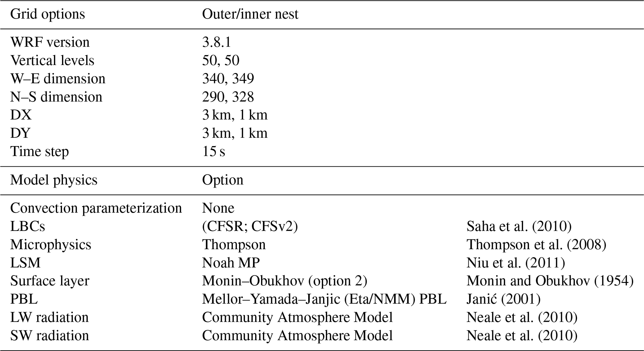
Saha et al. (2010)Thompson et al. (2008)Niu et al. (2011)Monin and Obukhov (1954)Janić (2001)Neale et al. (2010)Neale et al. (2010)Table 1Weather Research and Forecasting v3.8.1 (WRF) parameters used in this study, including the planetary boundary layer (PBL), long- and shortwave (LW and SW) radiation, land surface model (LSM), lateral boundary conditions (LBCs), grid spacing in the horizontal and vertical directions (DX and DY), and grid dimension in the west to east and north to south directions (W–E and N–S).
2.1 WRF model domain and configuration
We use the Weather Research and Forecasting version 3.8.1 (WRF; Skamarock et al., 2008; Powers et al., 2017) model with two nested domains. The inner domain has a 1 km resolution and 50 vertical levels, and the outer domain has a 3 km horizontal resolution. The inner-grid dimensions are 230 by 236 grid cells, the outer nest is 349 by 391 grid cells, and the integration time step is set to 15 s. We use the Climate Forecast System Reanalysis (CFSR) and Climate Forecast System Version 2 (CFSv2) before and after the 2011 (Saha et al., 2010) lateral boundary conditions. CFSR has a 0.5∘ horizontal grid resolution. The WRF “namelists” for configuring the model are provided in the Supplement. The outermost domain encompasses the majority of Colorado's Rocky Mountains, extending east into Kansas and as far west as the Uintas. Due to the time and computational constraints, each water year (1 October–30 September) is run independently and preceded by a 2-week spinup period. Consequently, multi-year soil–moisture or soil–atmosphere interactions might not be well represented, as the soil moisture fields (and other land surface states) are initialized at the beginning of each water year with the coarse CFSR soil moisture field. In this way, multiple water years can be run concurrently. The horizontal grid resolution of both domains is less than the 4 km typically considered necessary to permit convection (Weisman et al., 1997), so convective parameterizations are turned off. Additional WRF parameters are listed in Table 1.
In general, two predominant synoptic regimes control water inputs to the ERW, namely winter baroclinic waves (frontal systems) and summertime convective precipitation events that can sometimes be associated with the North American monsoon. Upper-level winds and moisture are predominantly from the west during the winter. The Colorado Front Range is also affected by upslope storms typified by northerly and easterly winds (Rasmussen et al., 1995). Streamflow hydrographs in the ERW are typified by a large single peaks during the spring and early summer, with occasional summer spikes, depending on the monsoonal precipitation and antecedent snow conditions, and gradually decay to baseflows in the late summer and fall (Carroll et al., 2020). The Colorado River system is undergoing a multi-decadal drought that is primarily driven by increased temperatures (Udall and Overpeck, 2017).
2.2 Comparison precipitation datasets
We compare WRF precipitation accumulations against the Natural Resources Conservation Service (NRCS) Snow Telemetry (SNOTEL) precipitation observations (Serreze et al., 1999). Analysis is conducted by water year (WY), which is from 1 October–30 September. SNOTEL stations are designed to provide cost-effective climate information for water-resource-important regions throughout the western USA and have been used extensively in the study of hydrology and climate. SNOTEL stations use both a snow pillow to measure snow accumulation mass and a separate, co-located precipitation gauge to measure the precipitation liquid equivalent. Ultimately, 23 SNOTEL sites are compared, ranging between 2400–3350 m above sea level (purple triangles in Fig. 1). The CFSR reanalyses used to force WRF do not assimilate SNOTEL precipitation data (Saha et al., 2010), so the precipitation recorded at the SNOTEL station is a completely independent check of the WRF precipitation at that grid cell. It is worth noting that there is a fundamental and unavoidable scale mismatch in making such a comparison, given that WRF grid cells are 1 km and that SNOTEL gauge orifices are less than a meter in diameter. Nevertheless this comparison is the best available for quantifying model precipitation performance and has been used as a benchmark in many other studies.
We also compare WRF precipitation fields against the Parameter Regression on Independent Slopes Model (PRISM; Daly et al., 2008), Livneh (Livneh et al., 2013), and Newman (Newman et al., 2015) geostatistical products, respectively. There are a number of differences between each model product, and elucidating the precise nature of the differences is beyond the scope of this article, but a brief description is warranted. One key difference is that PRISM and Newman use data from NRCS SNOTEL networks, whereas Livneh uses observations from the National Weather Service (NWS) Cooperative Observer Program (COOP) stations that have at least 20 years of data. Livneh precipitation accumulations are scaled such that the monthly means match mean PRISM climatology from 1961 to 1990. All three products use the PRISM terrain–precipitation relationships to distribute precipitation across terrain. PRISM uses a mapping methodology that regresses precipitation for each individual grid cell based on nearby station observations and terrain orientation with respect to climatic variables. Livneh and Newman are available until 2012 and 2013, respectively, whereas PRISM is available for the entire study period. It is also important and necessary to note the differences in grid resolution among the products. PRISM uses a 4 km × 4 km grid, the Livneh dataset is 0.0625∘ (∼ 6 km), and the Newman dataset is the coarsest at 0.125∘ (∼ 12 km). To compare the products at the regional scale, we use a bilinear interpolation as implemented in the xESMF Python package (https://xesmf.readthedocs.io/en/latest/, last access: 31 October 2023). WRF and each respective product are regridded to a common regular latitudinal and longitudinal grid, matching the coarser product's resolution with extents matching the WRF domain. A conservative regridding option was also tested, but we found that the results were very similar and had little impact on the overall interpretation.
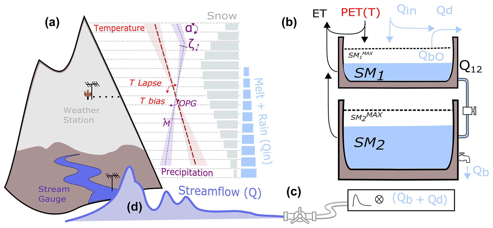
Figure 2Conceptual diagram illustrating the model used for the Bayesian inference approach. (a) Precipitation or temperature increase or decrease with elevation and snow accumulates or snowmelt based on temperature in each layer. Rain and snowmelt (Qin) and potential evapotranspiration (PET) calculated from temperature are fed into the hydrologic bucket model (b), with soil moisture in the top and bottom bucket, respectively (SM1, SM2), as state variables. Baseflow (Qb) and overland flow (Qd) are convolved with a routing kernel to produce streamflow (D) that can be compared to observations. Bayesian methods estimate the precipitation-distributing parameters conditioned on observed streamflow.
2.3 Bayesian reconstructions of ERW mean precipitation from streamflow
Estimating precipitation from streamflow observations, or “doing hydrology backwards” methods, have been employed in a number of studies (Kirchner, 2009; Pan and Wood, 2013), including those in snow-dominated alpine watersheds (Le Moine et al., 2015; Valery et al., 2009) and glaciated watersheds (Immerzeel et al., 2012), using glacier mass balance as opposed to streamflow. Henn et al. (2015) used a Bayesian inference method to evaluate gauge-based precipitation products, with further applications in Henn et al. (2016), Henn et al. (2018), and Hughes et al. (2020), the latter of which used such a methodology to evaluate atmospheric model performance for watersheds in the Sierra Nevada mountain range. The approach adopted in this study is intended to follow Henn et al. (2015) as closely as possible. In essence, the method combines a temperature index snow accumulation or ablation model run in elevation bands, a model accounting for soil water and a streamflow-routing bucket, and precipitation and temperature equations that distribute weather station observations upwards and downwards across elevation bands. Precipitation tends to increase with elevation, and temperature tends to decrease. A Bayesian inverse method finds the most likely ranges of the parameters, including parameters in the precipitation or temperature distributing functions that produce streamflow that best matches the observations. The precipitation in each elevation layer (at height z) is given by the following equation:
where Ps is the daily observed precipitation at a SNOTEL location (at height z0); Pbias is a precipitation gauge undercatch factor; OPG is the orographic precipitation gradient; m is a multiplicative error term; and , where z0 is the station elevation. Observations show that the snow water equivalent often decreases at high elevations in mountain watersheds (Kirchner et al., 2014) after increasing fairly linearly. This pattern is also seen in the ERW (see Sect. 3) and may be related to enhanced sublimation near ridges or a decrease in precipitation. Regardless of the cause, we introduce a new but simple model that can account for this using phenomena an effective layer elevation (zeff), which is proposed as follows:
where z is the height of the elevation layer. In this way, precipitation begins to decrease after a certain elevation ζ, with the slope defined by α. This relationship is graphically illustrated in Fig. 2. Other non-linear forms of the precipitation–elevation equation are frequently used (Liston and Elder, 2006), but we chose this novel, linear form for simplicity because it is found to match ASO data well. We use the SNOW-17 snow model (Anderson, 1973), which is run in discrete elevation layers to simulate the accumulation or melting of snow. In order to provide estimates that are as independent as possible of WRF, we use NRCS SNOTEL data from the Butte station located in the ERW to force the model. Periods of missing or poor-quality temperature data (a small percentage) are corrected using adjusted data from the Schofield station or interpolated between neighboring values. To infer precipitation, a three-part inference process is applied. In the first step, SNOW-17 parameters are calibrated for the Butte SNOTEL (380) site, including a precipitation undercatch term using an error minimization algorithm. Next, the OPG, ζ, α, and temperature lapse rate parameters are fitted to the mean Airborne Snow Observatory snow water equivalent (SWE) for water years 2018 and 2019. ASO produces 3 m scale estimates of snow water equivalent by taking repeated lidar observations of snow surfaces and modeling snow density using energy balance modeling. The spatial accuracy of ASO snow depths are on the order of centimeters (Deems et al., 2013). While ASO data present only a single snapshot in time, the spatial resolution and accuracy are very high and thus contain unparalleled information about the spatial distribution of orographic snowfall (Vögeli et al., 2016), while acknowledging that other factors (avalanches, wind redistribution, and sublimation) also control the snowpack depth prior to melt. The target ASO dates used are taken at our near-peak snow accumulation (early spring), so we expect that prior melt out is fairly minimal. Since we are using data averaged in elevation bands, the wind redistribution effects are also likely small.
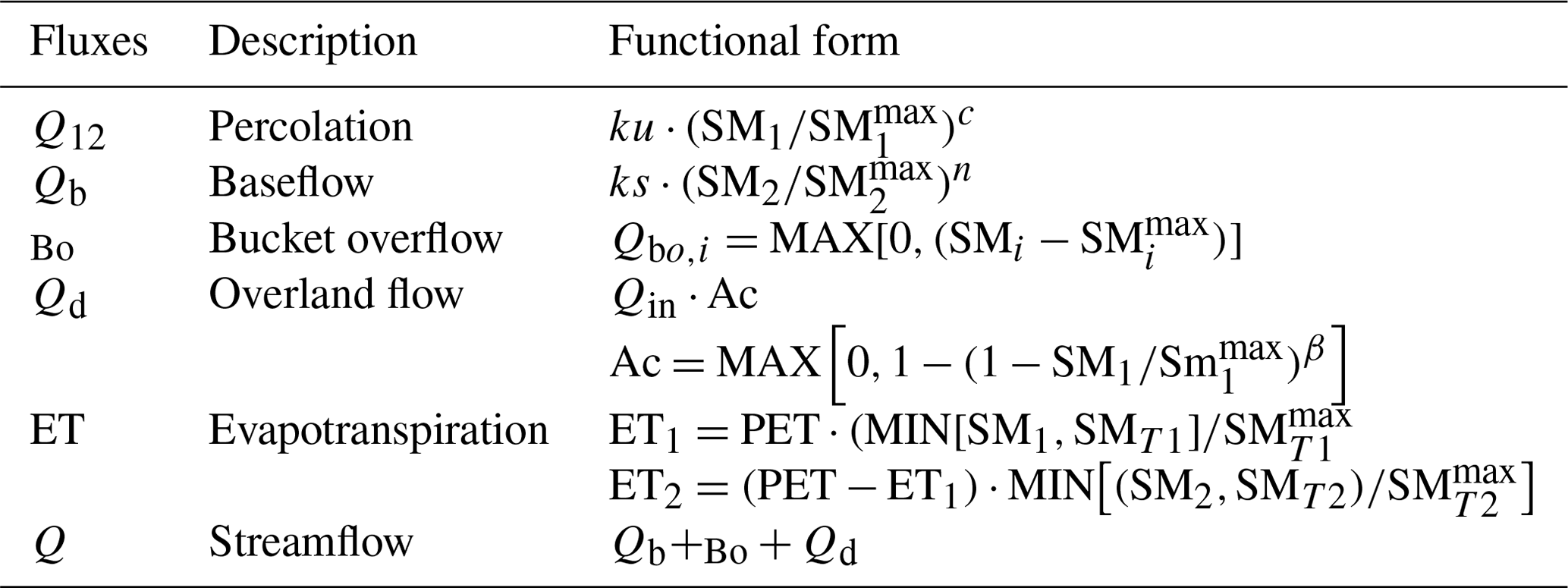
In the second step, SNOW-17 is coupled with a bucket hydrologic model, based on the FUSE hydrologic model framework Clark et al. (2008). SNOW-17 provides rain and snowmelt inputs to the hydrology model. The hydrologic model also requires a potential evapotranspiration (PET) forcing, which is computed using the Hamon formula (Hamon W. R., 1961). The model structure used in this study is the most similar to the VIC/PRMS forms described in Clark et al. (2008). The structure was chosen for simplicity and to have as few free parameters as possible. There are two state variables of soil moisture in the top and bottom buckets (SM1; SM2), with maximum capacities and . The model flux equations are solved sequentially, and time integration is performed with a basic forward Euler method, using a daily time step. The model flux equations are described in Table 2 and illustrated in Fig. 2. The evapotranspiration (ET) also depends on the fraction of water held in tension storage in the top and bottom layers (SMT1 and SMT2), which are simply given by . The summation of the bucket overflow (QBo), baseflow (QB), and direct or overland flow (Qd) is convolved with a routing function kernel to produce a streamflow that can be compared against USGS observations at the gauge site at the ERW outlet (Fig. 1).
The posterior model parameters (θ), conditioned on the model structure and observed streamflow data (d), can be expressed using Bayes' rule , where θ is the vector of model parameters, and d is the data. Analytical expressions for the posterior are not possible, so Markov chain Monte Carlo (MCMC) sampling methods are used, specifically the DEMetropolis algorithm implemented in the Python PyMC3 library (Salvatier et al., 2016). The model likelihood function P(d|θ) is a log-likelihood error function. We further employ a heteroscedastic error model, which states that the model residual is a normally distributed random variable with a standard deviation (σt) that grows linearly with discharge, following Henn et al. (2015) and Thyer et al. (2009). The model is given by , where Qt is the observed discharge at time step t. The coefficients of the error model are inferred along with model parameters. PyMC3 allows for a number of options for sampling from the posterior distribution. We found that a large number of samples (> 15 000) and multiple chains (or independent posterior samplings) led to better sampler convergences, as defined by the well-known Gelman–Rubin statistic implemented in PyMC3 (Gelman and Rubin, 1992). Example trace plots from the MCMC sampling are provided in the Supplement.
Bayesian parameter inference is performed in two parts. First, climatological or time-invariant parameters related to the subsurface hydrologic structure (Table 3) are inferred using precipitation and temperature that have been tuned to match ASO and SNOTEL observations. The assumption is that these conditions represent good approximations of the climatological behavior of the watershed. In the next step, the new posteriors of the time-invariant parameters are set as fixed, and meteorological parameters (Table 3) are inferred against discharge independently for each year, providing posterior likelihoods of precipitation that are conditioned on the model structure and streamflow data for that year.
While the details of the inference method are numerous, it is important to keep in mind the ultimate goal. We seek a Bayesian estimate of basin mean precipitation, independent of WRF and gridded precipitation products, that incorporates available high-quality hydrologic information to serve as an additional constraint on precipitation. The code for performing the analysis is posted publicly on GitHub (Rudisill, 2023a).
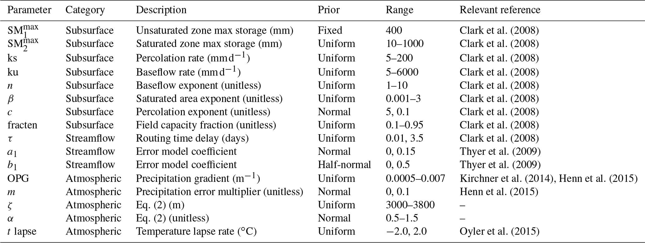
Clark et al. (2008)Clark et al. (2008)Clark et al. (2008)Clark et al. (2008)Clark et al. (2008)Clark et al. (2008)Clark et al. (2008)Clark et al. (2008)Clark et al. (2008)Thyer et al. (2009)Thyer et al. (2009)Kirchner et al. (2014)Henn et al. (2015)Henn et al. (2015)Oyler et al. (2015)Table 3Model parameter prior values and probability distribution used in the precipitation inference method. Ranges refer to the minimum or maximum of the uniform distribution or the mean or standard deviation of a normal distribution. Note that OPG is the orographic precipitation gradient.
3.1 Comparison against Liu et al. (2017)
First, to explore the fidelity of our WRF model configuration, we make a comparison against WRF v3.4.1 data from the Liu et al. (2017) 4 km dataset for water year 2013. This regional climate run covers the entirety of the continental United States and uses ERA-Interim initial and boundary conditions. Data are accessed from the National Center for Atmospheric Research (NCAR) data archive (Rasmussen and Liu, 2017). We compute the percent difference between the Liu et al. (2017) dataset and this dataset ( and find that there is generally good agreement between the datasets (Fig. 3). Our WRF configuration produces less precipitation in the center of the domain but more on the model boundaries, which is likely related to nesting effects or more finely resolved terrain in this dataset (1 km vs. 4 km). The average precipitation for the entire domain is ultimately quite similar (563 mm for this study versus 555 mm in Liu et al., 2017). This lends confidence to the overall skill of this particular WRF configuration and warrants further evaluation against other data sources.
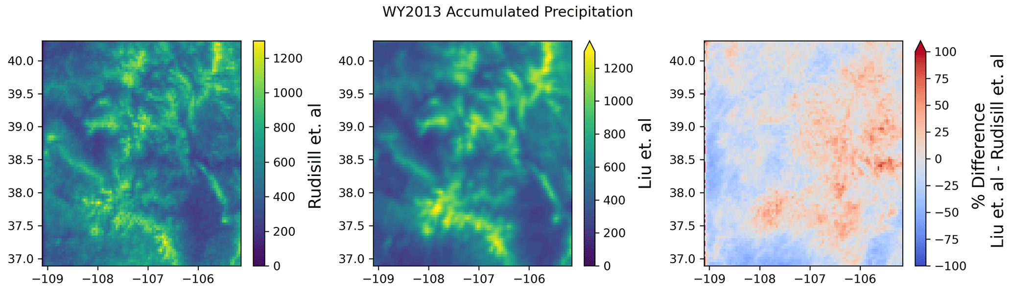
Figure 3Total accumulated model precipitation for water year 2013 from this study compared against data from the Liu et al. (2017) 4 km CONUS WRF dataset.
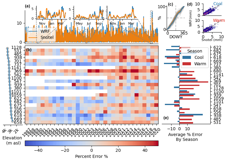
Figure 4Error characteristics of 24 SNOTEL sites compared against the corresponding WRF grid cells for 1987–2020. (a) The 1-week rolling mean time series of average SNOTEL (orange) precipitation compared against WRF (blue). (b) Annual precipitation percent error (SNOTEL as reference) for each site. (c) Average timing of water delivery (%) as a function of day of water year for WRF (blue) and SNOTEL (orange). (d) Correlations between 1-week accumulated precipitation in WRF and SNOTEL for the warm season (bottom) and cool season (top). (e) Average precipitation percent errors by season.
3.2 Seasonal precipitation accumulations compared against SNOTEL
WRF precipitation from the 34-year period is compared against corresponding SNOTEL grid cells shown in Fig. 4. Comparing WRF precipitation against SNOTEL observations demonstrates that WRF captures important features of atmospheric water delivery throughout the region. The analysis is divided into two rough categories, namely the cold season (October–March) and warm season (April–September), which are intended to roughly demarcate winter stratiform and summertime convective precipitation regimes. Analyzing the monthly averages of integrated vapor transport and 500 hPa wind directions shows that wind and moisture overwhelmingly come from the west during the cold season (October–April) and from the WSW during the remainder of the year (not shown). The percent errors in water year total precipitation, expressed as
are also examined. There is no immediately apparent trend in the location of SNOTEL site with respect to elevation or topography and error characteristics. The worst-performing site is Brumley (369), located on the lee side of a mountain ridge, where WRF overpredicts precipitation consistently throughout the study period. Interestingly, sites located only a few kilometers away on the windward side of the range are well predicted. While the correlations are similar between seasons, the errors in precipitation accumulation are not evenly distributed across the water year. During the warm season, WRF is wetter than SNOTEL sites for 16 of the 23 SNOTEL sites, with an average accumulated precipitation percent bias of 10.4 %. The cold-season percent error averaged across all years and SNOTEL locations is, remarkably, 0.264 % but with a 10.1 % standard deviation. Comparing the 1-week rolling mean time series of WRF averaged across all SNOTEL locations with the average SNOTEL precipitation shows good correlation (R2 of 0.85 and 0.88 for the warm and cold-season, respectively). The relationship between the binning window (daily–monthly) and correlation was also examined, and we found that correlations were low at the daily increments but tended to flatten beyond averaging window lengths greater than 3 to 4 d. There is no clear relationship between elevation and precipitation error.
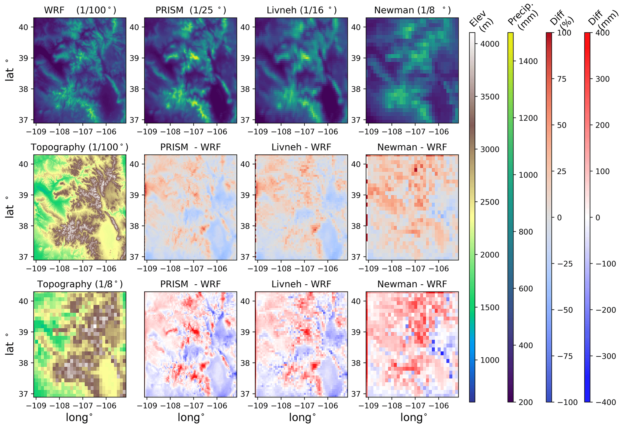
Figure 5The top row shows the spatial averages of 1987–2011 annual precipitation for the WRF, PRISM, Newman, and Livneh datasets for the entirety of the inner WRF model domain at each respective data resolution. Topography at WRF and the coarsest product resolution are also shown (far left column; second and third rows). The difference and percent difference between each product and WRF are shown in the second and third rows.
3.3 Regional comparison of WRF and gridded datasets
Three gridded precipitation datasets, namely the PRISM (4 km or ∼ ∘), Livneh (∘), and Newman (∘) products, are compared in Fig. 5 for water years between 1987 and 2012, as this is the time frame for which all data products are available. WRF is treated as the reference dataset, and the difference and percent error between each product are compared at the resolution of the coarsest product. For ease of comparison, we also bilinearly interpolate the curvilinear 1 km regular WRF grid onto a 0.01∘ regular latitudinal and longitudinal grid. The differences in topography between the high-resolution WRF grid and the coarsest grid (0.125∘) are also shown. The comparison of the water-year-averaged precipitation (1987–2012) shows significant differences between WRF and the gridded datasets, which are on the order of plus or minus 25 % and up to 400 mm in some regions. The differences among the gridded datasets are smaller, in particular between PRISM and Livneh. In general, WRF shows systematically less precipitation in the San Juan Mountains, Front Range, and Elk Mountains but sometimes more in the valleys and plateaus between ranges. PRISM shows a noticeable region of enhanced precipitation in the middle of the Elk Mountains (not far from the ERW) that is not as pronounced in the other geostatistical products. The differences between WRF and Newman are broadly similar to the other products, though WRF shows more precipitation in the southwestern corner of the domain around the Sangre de Cristo Mountains, whereas the opposite is true when compared against the other products. The mountain range is narrow and not well captured by the coarse scale of the topography at the 0.125∘ resolution.
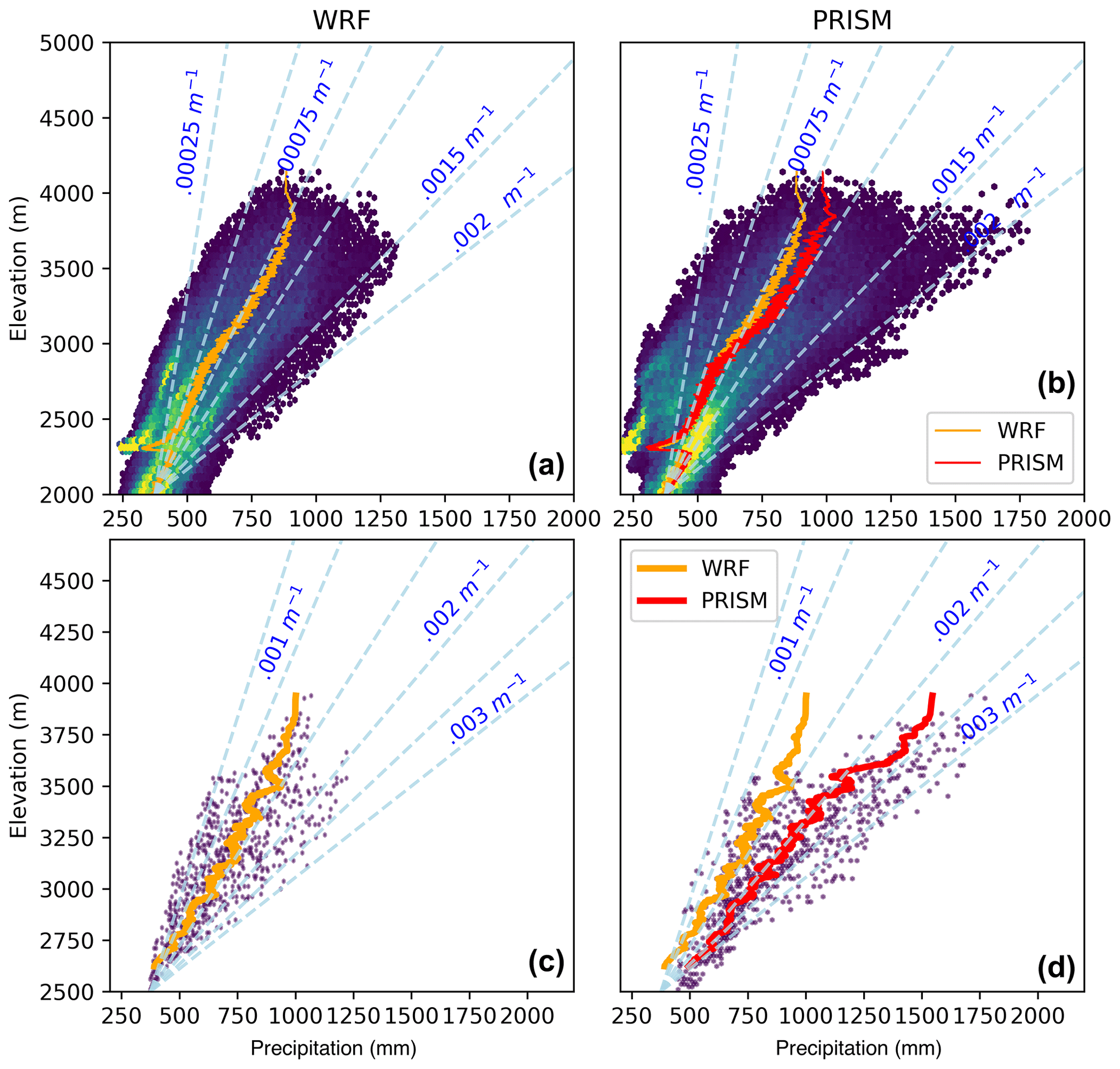
Figure 6Average annual precipitation versus elevation for WRF and PRISM for the entire WRF domain (a, b) and the ERW (c, d). Rolling means (solid lines) are shown. For comparison, constant OPG lines from Eq. (1), using a starting value of 300 mm at 2500 m of elevation, are also plotted.
Comparing precipitation as a function of terrain elevation (Fig. 6) shows that WRF typically has less precipitation at the highest elevations (greater than 3350 m) compared to PRISM and that the two datasets disagree the most in regions that are poorly sampled by SNOTEL locations (the SNOTEL maximum elevation is 3500 m). Livneh and Newman were also examined as functions of height but were ultimately very similar to the PRISM pattern and are not shown. PRISM has a more skewed distribution at higher elevations in addition to higher maxima than WRF. Both datasets show a clear rain-shadowing effect between 2250–2400 m, corresponding with the region to the east of the San Juan Mountains in the southeastern corner of the domain, although PRISM is drier than WRF (Fig. 5).
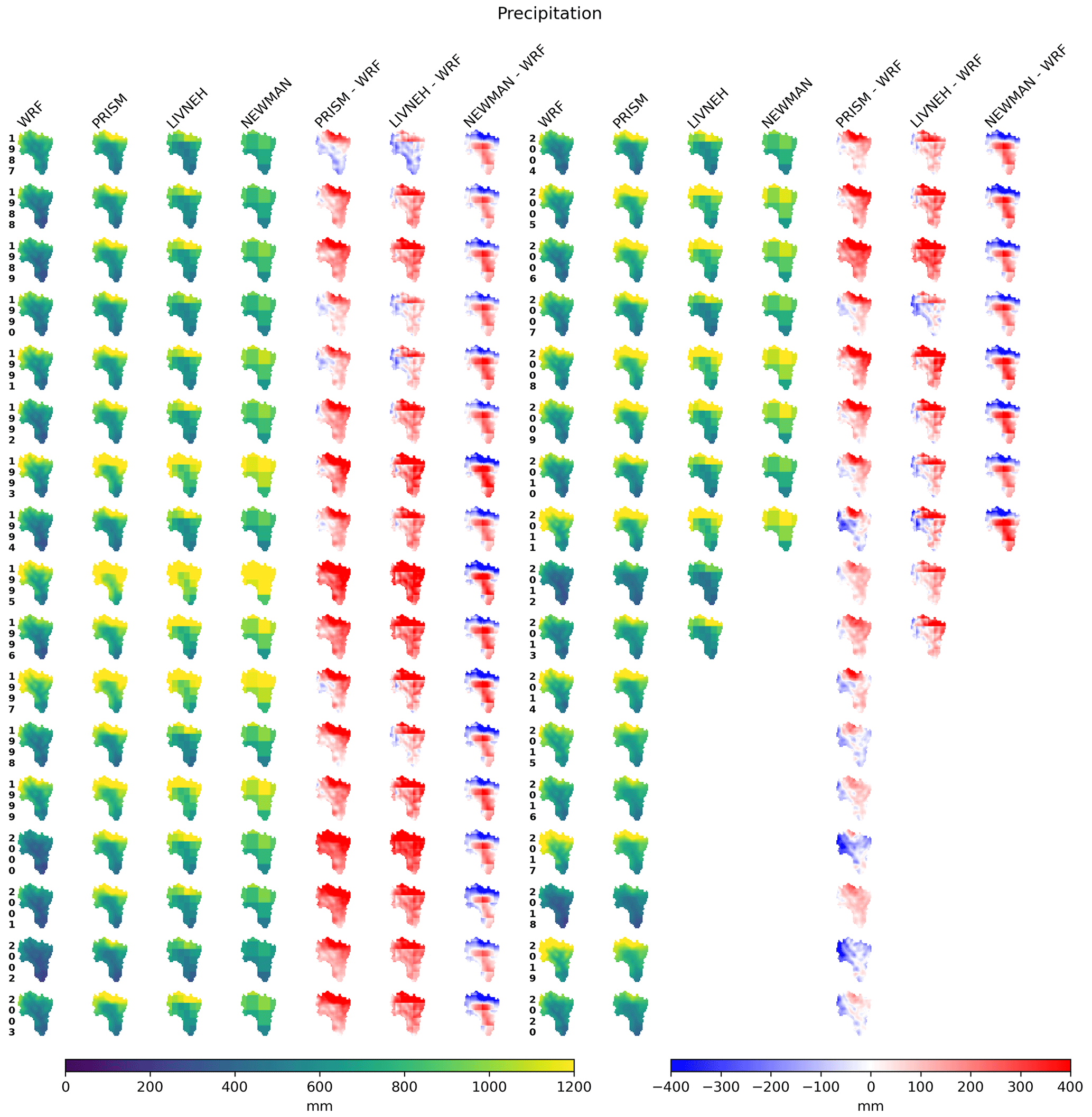
Figure 7ERW annual precipitation by water year (1987–2020) for WRF and PRISM, Livneh, and Newman precipitation products.
3.4 ERW precipitation analysis and reconstruction
To better understand the patterns and processes at the watershed scale, we examine precipitation estimates across the ERW. Unlike the regional comparisons, each product has been bilinearly interpolated to the 1 km × 1 km WRF grid. Figure 7 shows the clear effect of the resolution on the precipitation reconstruction in the ERW, as the Newman and Livneh datasets have much coarser textures than the others and do not reflect the underlying terrain very well. However, the ERW mean precipitation between Livneh and Newman is ultimately quite similar to PRISM, so consequently only PRISM and WRF are compared subsequently. WRF shows significantly less precipitation than any other product, particularly in the mid-1990s to early 2000s.
In order to better investigate some of the spatial characteristics of precipitation and relationships with terrain, we examine WRF and PRISM reconstructions for the warm and cold seasons averaged between water years 1987 and 2020. To do so, we define an enhancement factor for each grid cell, which is simply each grid cell normalized by the watershed mean value, as follows:
which is simply the ratio of the accumulated precipitation in each grid cell i,j to the m by n points averaged across the watershed.
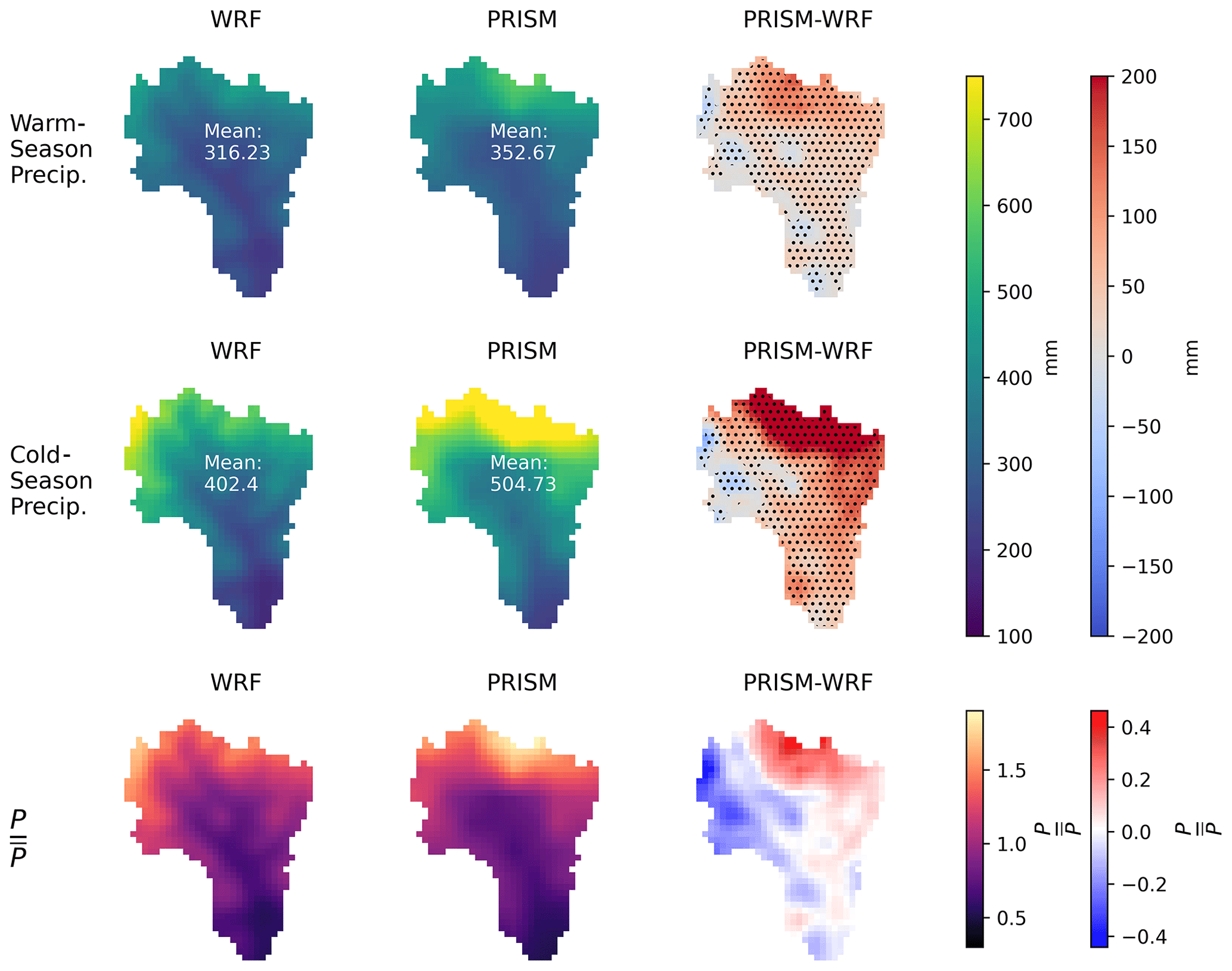
Figure 8Average cold season (October–April), warm season (April–October), and average annual precipitation in addition to the enhancement factor (precipitation normalized by the ERW mean precipitation) for WRF and PRISM across the ERW. Gray dots indicate regions with a difference that is statistically significant at the 95 % confidence level using a two-sided t test.
Both datasets show that more precipitation accumulates during the cold season on average. In many years, the mountain slopes on the windward side (west; left of the figure) receive more precipitation in WRF relative to PRISM (Fig. 8), despite having an overall lower precipitation. A two-sided t test shows that the difference in the mean precipitation between the two different datasets is statistically significant for the majority of the grid points, with the exception of a few small regions.
WRF has a much higher enhancement factor on the windward east side compared to PRISM, which has a very high enhancement factor and very high positive bias relative to WRF in the northwest. There does appear to be a significant downward shift in the PRISM basin mean precipitation in the final decade of the simulation, the causes of which are discussed in the next section. PRISM generally has a higher precipitation–elevation gradient compared to WRF for both the ERW and the entire WRF domain (Fig. 6). The averaged elevation–precipitation relationship is most similar at low to mid elevations and deviates most strongly at the highest elevations.
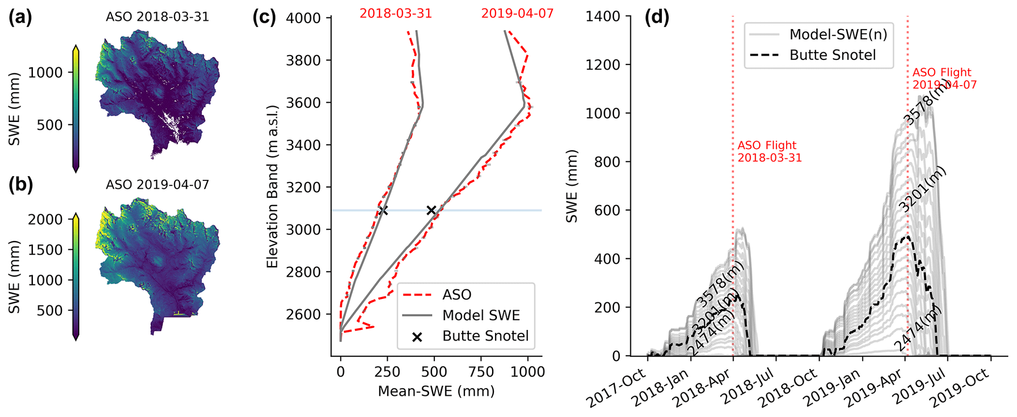
Figure 9(a, b) The Airborne Snow Observatory (ASO) SWE maps over the ERW employed in this study. (c) Basin-averaged elevation versus the average SWE for ASO and calibrated SNOW-17 at ASO flight dates. (d) Time series of calibrated SNOW-17 by elevation band (n=100).
Comparisons against Bayesian precipitation reconstructions
In order to better understand some of the discrepancies between WRF and the gridded datasets, a Bayesian precipitation inference method adapted from (Henn et al., 2015) is adapted to examine basin mean precipitation in the ERW. We analyze water years 1990–2020, as this is the time period in which high-quality USGS observations are available. Again, this method cannot isolate spatial precipitation patterns (which are significant; Fig. 8); only the basin mean precipitation is isolated. This is nonetheless useful, as the differences in the mean are large (∼ 150 mm). A three-part inference process is applied. First, SNOW-17 parameters are calibrated for the Butte SNOTEL (381; Fig. 1) site, including a precipitation undercatch term using a standard (non-Bayesian) error minimization algorithm (Pbias), as seen in Eq. (1). Given the relatively short number of model years, we choose to use the entire time series for calibration as opposed to splitting into calibration and validation periods, which is common but not always optimal in hydrologic contexts (Arsenault et al., 2018). Ad hoc splitting tests were performed, and there was not much impact on the final calibrated values. After calibration, SNOW-17 can capture the dynamics of snow accumulation and melt at the Butte SNOTEL site very well (see the Supplement). Next, the orographic precipitation gradient (OPG), temperature lapse rates, and precipitation gradient cutoff terms are calibrated against 2 years of Airborne Snow Observatory SWE products. The average ASO SWE from each elevation band is computed and compared against SNOW-17 run in elevation bands with the updated precipitation and temperature inputs. Water years 2018 and 2019 are low- and high-precipitation years, respectively, with approximately peak SWE values of greater than 2000 mm in 2019 and approximately 1000 mm in 2018 (Fig. 9). This is fortuitous, as these years represent high and low extremes and are thus good for bracketing the long-term average behavior. Aggregating SWE with respect to elevation bins shows a remarkably consistent increase in SWE with elevation, after which SWE values tend to decline. A similar pattern is found in the Tuolumne River basin in California (Henn et al., 2016; Fig. 4). Tuning the OPG gradient slope break (ζ) and decrease rate (α) in Eq. (2) allows for the fitting of the observed ASO SWE curves quite well. It is worth noting that the precipitation reduction term ultimately represents a small fraction of the total watershed area (less than 10 %). The calibrated OPG parameter is ultimately close to the initial guess of 0.002 m−1. This guess happens to be very close to the PRISM precipitation–terrain relationship (Fig. 6). The temporal evolution of SWE in the corresponding elevation bin also closely matches that of the SNOTEL site (Fig. 9c), demonstrating that this simple model can still capture key features of snow accumulation and ablation well.
Following the calibration of the SNOW-17 model parameters, the time-invariant subsurface and error model parameters are inferred using the Bayesian MCMC method from 1990—2020. The specific parameters are the subsurface parameters listed in Table 3. These parameters are related to geomorphic features of the watershed (soil depth, hydraulic conductivity, etc.) and are hypothesized to be largely unchanging during the study period. Extensive testing of the Bayesian inference approach found that sampler convergence criteria were satisfactorily met after treating the unsaturated zone maximum soil moisture storage as fixed. A value of 400 mm was chosen, reflecting approximately 1 m on average of sandy loam soil. The inference was performed with different fixed values of soil water storage, and we found there was ultimately little difference in the inferred values of other parameters. The baseline model skill is high at this stage, with an average root mean squared error of 0.65 mm prior to inferring precipitation forcing errors, suggesting that the model structure is a good approximation of the watershed dynamics. The MCMC trace plots and the prior and posterior time-invariant model parameters are shown in the Supplement.
After inferring the time-invariant subsurface model parameters, the meteorologic adjustment parameters are inferred on an annual basis against streamflow, with the mean posterior time-invariant subsurface model parameters inserted in the model and treated as fixed. This includes the precipitation error multipliers (m), OPG, OPG gradient slope break (ζ) elevation, and sensor temperature bias (atmospheric parameters in Table 3). The convergence of the posterior sampling for each case is evaluated using the Gelman–Rubin (Gelman and Rubin, 1992) statistic.
.
Figure 10Posterior and prior (blue dashed line) meteorological parameters inferred for each water year during 1990—2020. Each colored line is an independent posterior parameter distribution for each year.
Figure 11ERW basin mean precipitation for water years between 1990 and 2020 from three different estimates. WRF, PRISM, and the posterior probability distribution from the Bayesian MCMC inference method are shown. The widths of the PRISM and WRF bars are the standard error for the respective mean.
Figure 10 shows the priors and posterior parameter distributions for each water year. Interestingly, there are 1 or 2 years, where the inferred temperature lapse rate is positive. This is not completely nonphysical, as cold-air pools are very common in this watershed, particularly in the winter. We can now examine both the posterior model solutions for streamflow and the posterior probabilities of the basin mean precipitation for each year. A Gaussian kernel density estimate with a bandwidth of 2 mm is used to sample the posterior from each year and produce the plots in Fig. 11, showing the comparison with the inferred, WRF, and PRISM basin mean precipitation. There is considerable year-to-year variability in the relationship between the three estimates, but in general, the inference approach value lies in between the WRF and PRISM estimates.
Averaged across all years, the Bayesian inference method estimates 761 mm of precipitation, while WRF and PRISM estimate 725 mm and 862 mm, respectively. Consequently, WRF is slightly closer to the Bayesian inference reconstruction. For comparison, the average runoff from the ERW at the gauge outlet is 370 mm, so all estimates have a reasonable ratio of runoff to precipitation. The timing and magnitudes of the modeled streamflow compare well against the observed streamflow, lending confidence to the appropriateness of the model structure and parameter ranges (Fig. 12). Averaged across all years, the precipitation error multiplier has a mean close to 1, and OPG parameters are again close to the initial guess of 0.002 m−1 (not shown). The posterior solution model skill scores are high, indicating that the model captures the relevant watershed functions well. The entire discharge record has Kling–Gupta efficiencies (Gupta et al., 2009) greater than 0.9 (with 1 being a perfect match) and a root mean square difference (RMSD) of 0.524 mm d−1, which is an improvement from before.
Figure 12Observed streamflow compared against posterior model solutions of streamflow. The shaded region shows the 75 % model confidence intervals. Example water years are plotted on top to highlight details in the simulated hydrographs. The right panel shows the daily correlation between model and observed streamflow.
Further inspection of the data shows that the three estimates (WRF, PRISM, and inferred) tend to become approximately more alike after water year 2010. This change in behavior is almost certainly due to the addition of the Upper Taylor SNOTEL in water year 2010, immediately to the east of the ERW (Fig. 1), as PRISM uses this data source. Of the three SNOTEL sites closest to the ERW, Butte receives the least precipitation, Schofield the most (almost twice that of Butte), and Taylor typically receives a value in between the two. This relationship is illustrated in Fig. 13. The PRISM basin mean precipitation is a fairly constant +200 mm (standard deviation ∼ 60 mm) relative to the precipitation received at the Butte SNOTEL site, and the difference between the two values is significantly reduced after water year 2010 with the addition of the Upper Taylor site.
Figure 13ERW annual mean PRISM mean precipitation compared to the three closest SNOTEL sites, namely Schofield (737; north of ERW), Upper Taylor (1141; east of ERW), and Butte (381; within ERW). The pre- or post-2010 mean differences between the Butte and PRISM east mean are plotted with standard errors.
4.1 Comparisons against other regional climate reconstructions
Many other studies have evaluated WRF against SNOTEL and gridded precipitation datasets for the Colorado Rockies, though few have presented analyses for simulations spanning 3 decades. Rasmussen et al. (2011) report similar performance metrics between SNOTEL stations and WRF for a limited number of winter seasons. Jing et al. (2017) likewise found that wintertime precipitation accumulations compared against a number of SNOTEL sites was less than 15 %, using a 2 km WRF configuration with the North American Regional Reanalysis (NARR) boundary conditions. The absolute biases and percent differences between WRF and PRISM from this study are similar to both the Jing et al. (2017) 2 km WRF and 4 km WRF results from Liu et al. (2017), which are both presented in Fig. 7 found in Jing et al. (2017). Similar performance against SNOTEL is also reported in Gutmann et al. (2012), who examined winter-only precipitation, using a 2 km WRF configuration and again using the NARR boundary conditions. The similarity of results is interesting, since there are differences in resolutions, nesting configurations, model code versions, boundary conditions, microphysical schemes, and other options among all of these models. It is generally recognized that RCM precipitation is sensitive to parameterization options, which we do not explicitly test here. However, Xu et al. (2023) performed sensitivity analyses using the same physics options and boundary conditions as those used in this study (called BSU-WRF in their paper) and found that this configuration performed better for simulating near-surface climate than several other configurations for water year 2019 across the ERW and that the choice of lateral boundary conditions (LBCs) was less important than physics options for simulating meteorology across the ERW.
Differences in error behavior between cold and warm seasons can likely be attributed to precipitation generating regimes. WRF has a lower weekly correlation with SNOTEL stations (lower R2 value) and higher percent errors. Additional analysis shows that the warm season bias is related to an excessive number of wet days relative to SNOTEL during the warm season. Jing et al. (2017) likewise found that the WRF skill decreased in April, which is concurrent with an increase in convective available potential energy in the atmosphere. Surface heating tends to increase during the warmer months, leading to convective instabilities and localized precipitation, when compared to more uniform stratiform precipitation during the winter (Dai, 2006). At the same time, the nature of errors at the gauge locations can depend on the phase of falling hydrometeors (rain versus snow), as snowflakes have slower fall speeds and are more subject to undercatch during stronger winds (Goodison et al., 1998; Harpold et al., 2017). It is even more interesting that cold-season errors are lower than warm-season errors, as the gauge errors are expected to be higher in the cold season when more precipitation falls as snow. Some studies have attempted to account for gauge undercatch at SNOTEL sites using the co-located snow pillow SWE measurements and wind observations, but these methods are not employed here for the precipitation evaluation (Livneh et al., 2013; Sun et al., 2019). However, an undercatch term (Pbias) for the Butte SNOTEL was used in the precipitation inference method, but the value was small (< 1 mm), and only 2 out of the 30 years examined appeared to show snow water equivalent values greater than the co-located accumulated precipitation. The overestimation of the number of wet days is well known in both regional and global climate modeling (Maraun et al., 2010; Chen et al., 2021). However, it is difficult to determine the extent of the potential drizzle bias, given the relatively low resolution (daily; 2.54 mm) of SNOTEL gauges. The NRCS provides recent data with sub-daily frequency but not for the entirety of the analysis period. Additional comparisons with other high-resolution gauge data may shed light on some of these questions. Additional experiments may consider indirect data sources (soil moisture and remote sensing) to better understand modeling drizzle days in regions covered by SNOTEL, which account for ∼ 10 % of annual WRF precipitation. Users of regional climate model precipitation may consider performing bias correction by removing low-precipitation days (Maraun et al., 2010).
4.2 Timescales and data non-stationarity
This study illustrates some of the challenges of multi-decadal model evaluations and highlights the utility of using streamflow observations as additional long-term water balance indicators. The WRF dataset covered 1987–2020, whereas the Livneh and Newman datasets were only compared up until 2012 because of data coverage. Moreover, only 14 of the 23 regionally relevant SNOTEL sites existed for the entire data period. Streamflow, on the other hand, can often have much longer records (Tillman et al., 2022). This study demonstrates that streamflow can be a useful data point for evaluating precipitation budgets, given that comparisons of gridded precipitation datasets are imperfect. This might be particularly true for data-poor regions, where there are not as many high-elevation precipitation measurements, and globally spanning datasets, such as WorldClim (Fick and Hijmans, 2017) or other globally spanning products (Araghi et al., 2021), are likely subject to greater uncertainties. The step change in the PRISM basin mean precipitation after approximately water year 2010 (Fig. 13) underscores the fact that caution must be taken when analyzing precipitation trends from gridded datasets, as the inclusion of different stations can induce spurious trends. For instance, the annual ERW mean precipitation from PRISM from 1987–2020 shows a negative trend with p = 0.06 and R2 = 0.33, which likely reflects the addition of the Taylor SNOTEL site. The fact that PRISM more closely matches the WRF and inferred precipitation data (two independent estimates) in the last decade, after the addition of a nearby gauge, lends more confidence to the WRF-modeled precipitation in the early parts of the simulation. A similar conclusion was also reached in Gutmann et al. (2012). That being said, WRF still typically underestimates precipitation at the Schofield SNOTEL site (737; Fig. 4), so the low bias may carry over to adjacent regions within ERW. Moreover, the LBC conditions change from the CFSR (Saha et al., 2010) to the CFSv2 analysis (Saha et al., 2014) after 2011. Regional climate models are ultimately dependent on the boundary conditions (Goergen and Kollet, 2021), so changes in data assimilation and reanalyses methodologies likely influence the character of the boundary conditions and the results. The quality and quantity of data assimilation greatly increases during the late 1990s and early 2000s (Saha et al., 2010), in addition to there being model structural changes between data products. It is possible that this is the reason that the WRF precipitation tends to transition from low biased to high biased when evaluated against SNOTEL during the late 2000s.
4.3 Interpreting Bayesian precipitation reconstructions
Combining snow remote sensing, streamflow observations, and parsimonious hydrologic models in a Bayesian framework allows for creating novel constraints on watershed average precipitation that leverage both the high spatial resolution of ASO snow data and long records of streamflow. Henn et al. (2016) likewise used ASO data in a joint-inference method in the Tuolumne River watershed and found that doing so reduced the dependence of inferred precipitation on hydrologic model structure, when compared with inferring precipitation from streamflow alone. That being said, uncertainties in soil parameters, PET forcing, and water limitation relationships in the PET–ET relationships do limit the conclusions drawn from the precipitation inference approach. ET is directly related to inferred precipitation by the hydrologic mass budget equation, , so holding Q and constant implies that higher annual inferred precipitation requires higher annual ET. During the long-term hydrologic parameter inference, the parameter determining soil moisture held in tension (fracten) consistently converged towards the limit of 1 (a lower-ET solution). Additional sensitivity experiments show that higher-ET solutions (lower fracten) tended to smooth spring and early summer streamflow peaks excessively when compared to observations, suggesting some confidence in the ET solution. For these reasons, it is also unlikely that a PET forcing parameterization has significant impact on the overall water budgeting, as the soil moisture availability term also has a significant impact on actual ET.
Observations and independent modeling studies shed some light on the question of basin-wide ET. Ryken et al. (2021) reported 450–550 mm yr1 of ET, which is interpreted as being an upper limit of the basin-wide ET, as the observations were located in a well-watered riparian corridor. Carroll et al. (2019) estimated the ET for a high-elevation sub-watershed of the upper ERW as being over 623 ± 50 mm yr1, and Tran et al. (2019) found ET values between 431 and 624 mm yr1 for the same watershed extent as in this study. This is closer to, but still higher than, the average of 388 ± 50 mm that is found from the inference method presented here. However, the Tran et al. (2019) study used PRISM precipitation input, and a different precipitation dataset (such as WRF) may produce a different result, as ET depends on the antecedent precipitation.
Another major assumption is that parameters in the precipitation distribution functions are constant for each season. Future efforts could consider inferring precipitation error parameters for individual storm events, such as in Le Moine et al. (2015) and Koskela et al. (2012). Moreover, while this study demonstrated that airborne snow lidar products can be incorporated into a Bayesian inference strategy to evaluate orographic precipitation, the potential applications are vast. This study only used one-dimensional SWE versus elevation information as part of the Bayesian inference framework to calibrate the climatological OPG parameter in Eq. (2.3). A cursory analysis shows that the patterns of SWE from the ASO data (Fig. 9a) are very similar to the relative precipitation enhancement from WRF, where the largest values of precipitation or snow are on the windward (western) ridge the watershed. This region also happens to generally be the furthest from observations, so ASO provides a very unique window into the spatial water budgets of this region and supports the precipitation enhancement shape that is modeled by WRF. This study only used the Bayesian inference approach for the ERW, but similar methods could be applied to all headwaters basins in the domain without significant anthropogenic disturbances. Modern software packages such as PyMC3 (Salvatier et al., 2016) are well developed infrastructures that make implementing MCMC calculations significantly easier than ad hoc approaches.
This study examined 34 years of precipitation from a high-resolution (1 km × 1 km) regional climate model (WRF v3.8.1). The precipitation is compared against the information in the Liu et al. (2017) dataset, SNOTEL observations, three different precipitation products (PRISM, Livneh, and Newman), and basin mean precipitation inferred from a Bayesian inference method that uses streamflow and high-resolution snow lidar remote-sensing data (Painter et al., 2016). The primary goal is to better characterize precipitation biases and error characteristics from this regional climate model simulation, while acknowledging that gridded precipitation estimates are models themselves and subject to large uncertainties. We showed the following:
-
WRF has an average of 0.246 % bias (s = 13.63 %) during the cold season and an average of 10.37 % (s = 12.79 %) bias during the warm season when averaged across 24 SNOTEL stations, suggesting that cold-season precipitation is better predicted, despite being more difficult to accurately observe due to undercatch effects.
-
PRISM, Livneh, and Newman show generally similar patterns and disagree with WRF (on the order of ± 20 % per year). The largest disagreements are at the highest elevations above the SNOTEL measurement network elevation.
-
WRF is slightly closer to a Bayesian reconstruction of basin mean precipitation than the PRISM estimate. Combining multiple sources of hydrologic information in a Bayesian framework proves to be a useful data point for model evaluation.
-
WRF shows a spatial pattern of precipitation enhancement in the ERW that more closely matches patterns found in high-resolution snow remote-sensing data (ASO) compared to that of PRISM.
-
Some geostatistical, grid-based products are influenced by the change in the spatial density of gauges over time and should be treated with care for long-term model evaluations.
Many of the insights about the uncertainties in mountain precipitation have been made in other studies (Lundquist et al., 2019; Henn et al., 2018; Daly et al., 2008). While they serve a clear purpose for model development, the limitations of gridded precipitation data in mountain terrain should be carefully considered, particularly when high-resolution modeling strategies (enhanced parameterizations, fine-scale grid spacings, etc.) are employed. Using high-quality, non-traditional hydrologic indicators (such as snow remote sensing) should be a priority for regional climate simulation development.
The codes for performing the analysis, Bayesian reconstruction and hydrologic bucket model, and creating the figures are publicly available on GitHub (Rudisill, 2023a). The authors developed a Python wrapper for running the WRF model on high-performance computing (HPC) systems for this project, which is available from https://doi.org/10.5281/zenodo.10058594 (Rudisill, 2023b).
A subset of the WRF RCM dataset covering the ERW is available on the Environmental System Science Data Infrastructure for a Virtual Ecosystem (ESS-DIVE) repository (https://doi.org/10.15485/1845448, Rudisill et al., 2022). We are working on making the entire WRF dataset publicly available, and researchers are encouraged to reach out to the corresponding author about data availability. USGS streamflow data were downloaded from the package at https://doi.org/10.5066/P9X4L3GE (DeCicco et al., 2023). NRCS SNOTEL data were downloaded from https://doi.org/10.5281/zenodo.8045105 (Rudisill, 2023c). Livneh precipitation data are available from https://psl.noaa.gov/data/gridded/data.livneh.html (NOAA Physical Sciences Laboratory, 2021). Newman data are available from https://doi.org/10.5065/D6TH8JR2 (Climate Data Gateway at NCAR, 2018). PRISM data are available from https://prism.oregonstate.edu/ (PRISM Climate Group, 2021). ASO data were downloaded from the National Snow and Ice Data center at https://doi.org/10.5067/STOT5I0U1WVI (Painter, 2018). CFSR and CFSv2 were downloaded from https://www.ncei.noaa.gov/thredds/catalog.html (last access: 31 October 2023; Saha et al., 2010, 2014).
The supplement related to this article is available online at: https://doi.org/10.5194/gmd-16-6531-2023-supplement.
WR ran the WRF simulations, compiled data, performed the analysis, developed the Bayesian reconstruction methodology, and wrote the paper. AF provided funding and developed the WRF configuration options. RC provided expertise on the hydrology and climate of the ERW and edited the paper.
The contact author has declared that none of the authors has any competing interests.
Publisher's note: Copernicus Publications remains neutral with regard to jurisdictional claims made in the text, published maps, institutional affiliations, or any other geographical representation in this paper. While Copernicus Publications makes every effort to include appropriate place names, the final responsibility lies with the authors.
William Rudisill and Alejandro Flores acknowledge funding from the Department of Energy (DOE) Biological and Environmental Research (BER; grant no. DOE:DE-SC0019222). This research made use of Idaho National Laboratory computing resources, which are supported by the Office of Nuclear Energy of the U.S. Department of Energy and the Nuclear Science User Facilities (grant no. DE-AC07-05ID14517). We also acknowledge high-performance computing support of the R2 compute cluster (https://doi.org/10.18122/B2S41H, Boise State's Research Computing Department, 2017) provided by Boise State University's Research Computing Department.
This research has been supported by the Biological and Environmental Research (grant no. DE-SC0019222).
This paper was edited by Di Tian and reviewed by two anonymous referees.
Anderson, E. A.: National Weather Service River Forecast System: Snow Accumulation and Ablation Model, U. S. Department of Commerce, National Oceanic and Atmospheric Administration, National Weather Service, 1973. a
Araghi, A., Jaghargh, M. R., Maghrebi, M., Martinez, C. J., Fraisse, C. W., Olesen, J. E., and Hoogenboom, G.: Investigation of satellite-related precipitation products for modeling of rainfed wheat production systems, Agric. Water Manage., 258, 107222, https://doi.org/10.1016/j.agwat.2021.107222, 2021. a
Arsenault, R., Brissette, F., and Martel, J.-L.: The hazards of split-sample validation in hydrological model calibration, J. Hydrol., 566, 346–362, 2018. a
Ashouri, H., Hsu, K.-L., Sorooshian, S., Braithwaite, D. K., Knapp, K. R., Dewayne Cecil, L., Nelson, B. R., and Prat, O. P.: PERSIANN-CDR: Daily Precipitation Climate Data Record from Multisatellite Observations for Hydrological and Climate Studies, B. Am. Meteorol. Soc., 96, 69–83, 2015. a
Boise State's Research Computing Department: R2: Dell HPC Intel E5v4 (High Performance Computing Cluster). Boise, ID: Boise State University, https://doi.org/10.18122/B2S41H, 2017. a
Carroll, R. W. H., Deems, J. S., Niswonger, R., Schumer, R., and Williams, K. H.: The importance of interflow to groundwater recharge in a snowmelt-dominated headwater basin, Geophys. Res. Lett., 46, 5899–5908, 2019. a
Carroll, R. W. H., Gochis, D., and Williams, K. H.: Efficiency of the summer monsoon in generating streamflow within a snow-dominated headwater basin of the Colorado river, Geophys. Res. Lett., 47, e2020GL090856, https://doi.org/10.1029/2020GL090856, 2020. a
Chen, D., Dai, A., and Hall, A.: The convective-to-total precipitation ratio and the “drizzling” bias in climate models, J. Geophys. Res., 126, e2020JD034198, https://doi.org/10.1029/2020JD034198, 2021. a
Clark, M. P., Slater, A. G., Rupp, D. E., Woods, R. A., Vrugt, J. A., Gupta, H. V., Wagener, T., and Hay, L. E.: Framework for Understanding Structural Errors (FUSE): A modular framework to diagnose differences between hydrological models: DIFFERENCES BETWEEN HYDROLOGICAL MODELS, Water Resour. Res., 44, 1–14, https://doi.org/10.1029/2007WR006735, 2008. a, b, c, d, e, f, g, h, i, j, k
Climate Data Gateway at NCAR: Gridded Ensemble Precipitation and Temperature Estimates over the Contiguous United States Version 2.0, NCAR [data set], https://doi.org/10.5065/D6TH8JR2, 2018. a
Currier, W. R., Thorson, T., and Lundquist, J. D.: Independent Evaluation of Frozen Precipitation from WRF and PRISM in the Olympic Mountains, J. Hydrometeorol., 18, 2681–2703, 2017. a
Dai, A.: Precipitation Characteristics in Eighteen Coupled Climate Models, J. Climate, 19, 4605–4630, 2006. a
Daly, C., Halbleib, M., Smith, J. I., Gibson, W. P., Doggett, M. K., Taylor, G. H., Curtis, J., and Pasteris, P. P.: Physiographically sensitive mapping of climatological temperature and precipitation across the conterminous United States, Int. J. Climatol., 28, 2031–2064, 2008. a, b, c
de Boer, G., White, A., Cifelli, R., Intrieri, J., Hughes, M., Mahoney, K., Meyers, T., Lantz, K., Hamilton, J., Currier, W., Sedlar, J., Cox, C., Hulm, E., Riihimaki, L. D., Adler, B., Bianco, L., Morales, A., Wilczak, J., Elston, J., Stachura, M., Jackson, D., Morris, S., Chandrasekar, V., Biswas, S., Schmatz, B., Junyent, F., Reithel, J., Smith, E., Schloesser, K., Kochendorfer, J., Meyers, M., Gallagher, M., Longenecker, J., Olheiser, C., Bytheway, J., Moore, B., Calmer, R., Shupe, M. D., Butterworth, B., Heflin, S., Palladino, R., Feldman, D., Williams, K., Pinto, J., Osborn, J.,Costa, D., Hall, E., Herrera, C., Hodges, G., Soldo, L., Stierle, S., and Webb, R. S.: Supporting Advancement in Weather and Water Prediction in the Upper Colorado River Basin: The SPLASH Campaign, B. Am. Meteorol. Soc., 1, E1853–E1874, https://doi.org/10.1175/BAMS-D-22-0147.1, 2023. a
DeCicco, L., Hirsch, R., Lorenz, D., Watkins, D., and Johnson, M.: dataRetrieval: R packages for discovering and retrieving water data available from U.S. federal hydrologic web services, 2.7.13, U.S. Geological Survey, Reston, VA [code], https://doi.org/10.5066/P9X4L3GE, 2023. a
Deems, J. S., Painter, T. H., and Finnegan, D. C.: Lidar measurement of snow depth: a review, J. Glaciol., 59, 467–479, 2013. a
Feldman, D., Boos, A. A. W., Chandrasekar, R. C. V., Collis, W. C. S., De Mott, J. D. P., Flores, J. F. A., Harrington, D. G. J., Kumijian LR Leung, M., Raleigh, T. O. M., Mc Kenzie Skiles J Smith R Sullivan, A. R. S., Varble, P. U. A., and Williams, K.: Surface Atmosphere Integrated Field Laboratory (SAIL) Science Plan Tech. Rep. No. DOE/SC-ARM-21-004, Tech. Rep. DOE/SC-ARM-21-004, U. S. Department of Energy, Office of Science, Biological and Environmental Research Program, USA, 2021. a
Fick, S. E. and Hijmans, R. J.: WorldClim 2: new 1-km spatial resolution climate surfaces for global land areas, Int. J. Climatol., 37, 4302–4315, 2017. a
Gelman, A. and Rubin, D. B.: Inference from Iterative Simulation Using Multiple Sequences, Stat. Sci., 7, 457–472, 1992. a, b
Goergen, K. and Kollet, S.: Boundary condition and oceanic impacts on the atmospheric water balance in limited area climate model ensembles, Sci. Rep., 11, 6228, https://doi.org/10.1038/s41598-021-85744-y, 2021. a
Goodison, B. E., Louie, P. Y. T., and Yang, D.: WMO solid precipitation measurement intercomparison, World Meteorological Organization, Geneva, Switzerland, 212 pp., 1998. a
Gupta, H. V., Kling, H., Yilmaz, K. K., and Martinez, G. F.: Decomposition of the mean squared error and NSE performance criteria: Implications for improving hydrological modelling, J. Hydrol., 377, 80–91, 2009. a
Gutmann, E. D., Rasmussen, R. M., Liu, C., Ikeda, K., Gochis, D. J., Clark, M. P., Dudhia, J., and Thompson, G.: A Comparison of Statistical and Dynamical Downscaling of Winter Precipitation over Complex Terrain, J. Climate, 25, 262–281, 2012. a, b, c, d
Hamon W. R.: Estimating Potential Evapotranspiration, J. Hydr Eng. Div.-ASCE, 87, 107–120, 1961. a
Harpold, A. A., Kaplan, M. L., Klos, P. Z., Link, T., McNamara, J. P., Rajagopal, S., Schumer, R., and Steele, C. M.: Rain or snow: hydrologic processes, observations, prediction, and research needs, Hydrol. Earth Syst. Sci., 21, 1–22, https://doi.org/10.5194/hess-21-1-2017, 2017. a
Henn, B., Clark, M. P., Kavetski, D., and Lundquist, J. D.: Estimating mountain basin-mean precipitation from streamflow using Bayesian inference, Water Resour. Res., 51, 8012–8033, 2015. a, b, c, d, e, f
Henn, B., Clark, M. P., Kavetski, D., McGurk, B., Painter, T. H., and Lundquist, J. D.: Combining snow, streamflow, and precipitation gauge observations to infer basin-mean precipitation, Water Resour. Res., 52, 8700–8723, 2016. a, b, c, d
Henn, B., Newman, A. J., Livneh, B., Daly, C., and Lundquist, J. D.: An Assessment of Differences in Gridded Precipitation Datasets in Complex Terrain, J. Hydrol., 556, 1205–1219, 2018. a, b, c
Hubbard, S. S., Williams, K. H., Agarwal, D., Banfield, J., Beller, H., Bouskill, N., Brodie, E., Carroll, R., Dafflon, B., Dwivedi, D., Falco, N., Faybishenko, B., Maxwell, R., Nico, P., Steefel, C., Steltzer, H., Tokunaga, T., Tran, P. A., Wainwright, H., and Varadharajan, C.: The East River, Colorado, watershed: A mountainous community testbed for improving predictive understanding of multiscale hydrological–biogeochemical dynamics, Vadose Zone J., 17, 1–25, 2018. a, b
Hughes, M., Lundquist, J. D., and Henn, B.: Dynamical downscaling improves upon gridded precipitation products in the Sierra Nevada, California, Clim. Dynam., 55, 111–129, 2020. a
Ikeda, K., Rasmussen, R., Liu, C., Gochis, D., Yates, D., Chen, F., Tewari, M., Barlage, M., Dudhia, J., Miller, K., Arsenault, K., Grubišić, V., Thompson, G., and Guttman, E.: Simulation of seasonal snowfall over Colorado, Atmos. Res., 97, 462–477, 2010. a, b
Immerzeel, W. W., Pellicciotti, F., and Shrestha, A. B.: Glaciers as a proxy to quantify the spatial distribution of precipitation in the Hunza basin, Mt. Res. Dev., 32, 30–38, 2012. a
Immerzeel, W. W., Lutz, A. F., Andrade, M., Bahl, A., Biemans, H., Bolch, T., Hyde, S., Brumby, S., Davies, B. J., Elmore, A. C., Emmer, A., Feng, M., Fernández, A., Haritashya, U., Kargel, J. S., Koppes, M., Kraaijenbrink, P. D. A., Kulkarni, A. V., Mayewski, P. A., Nepal, S., Pacheco, P., Painter, T. H., Pellicciotti, F., Rajaram, H., Rupper, S., Sinisalo, A., Shrestha, A. B., Viviroli, D., Wada, Y., Xiao, C., Yao, T., and Baillie, J. E. M.: Importance and vulnerability of the world's water towers, Nature, 577, 364–369, 2020. a
Janić, Z. I.: Nonsingular implementation of the Mellor-Yamada level 2.5 scheme in the NCEP Meso model, Tech. rep., National Centers for Environmental Prediction Office, USA, 2001. a
Jing, X., Geerts, B., Wang, Y., and Liu, C.: Evaluating Seasonal Orographic Precipitation in the Interior Western United States Using Gauge Data, Gridded Precipitation Estimates, and a Regional Climate Simulation, J. Hydrometeorol., 18, 2541–2558, 2017. a, b, c, d
Kirchner, J. W.: Catchments as simple dynamical systems: Catchment characterization, rainfall-runoff modeling, and doing hydrology backward: CATCHMENTS AS SIMPLE DYNAMICAL SYSTEMS, Water Resour. Res., 45, W02429, https://doi.org/10.1029/2008wr006912, 2009. a
Kirchner, P. B., Bales, R. C., Molotch, N. P., Flanagan, J., and Guo, Q.: LiDAR measurement of seasonal snow accumulation along an elevation gradient in the southern Sierra Nevada, California, Hydrol. Earth Syst. Sci., 18, 4261–4275, https://doi.org/10.5194/hess-18-4261-2014, 2014. a, b
Koskela, J. J., Croke, B. W. F., Koivusalo, H., Jakeman, A. J., and Kokkonen, T.: Bayesian inference of uncertainties in precipitation-streamflow modeling in a snow affected catchment, Water Resour. Res., 48, W11513, https://doi.org/10.1029/2011WR011773, 2012. a
Le Moine, N., Hendrickx, F., Gailhard, J., Garçon, R., and Gottardi, F.: Hydrologically Aided Interpolation of Daily Precipitation and Temperature Fields in a Mesoscale Alpine Catchment, J. Hydrometeorol., 16, 2595–2618, 2015. a, b
Lettenmaier, D. P., Alsdorf, D., Dozier, J., Huffman, G. J., Pan, M., and Wood, E. F.: Inroads of remote sensing into hydrologic science during the WRR era, Water Resour. Res., 51, 7309–7342, 2015. a
Lin, Y. and Mitchell, K. E.: 1.2 the NCEP stage II/IV hourly precipitation analyses: Development and applications, in: Proceedings of the 19th Conference Hydrology, American Meteorological Society, 9–13 January 2005, San Diego, CA, USA, vol. 10, Citeseer, 2005. a
Liston, G. E. and Elder, K.: A Meteorological Distribution System for High-Resolution Terrestrial Modeling (MicroMet), J. Hydrometeorol., 7, 217–234, 2006. a
Liu, C., Ikeda, K., Rasmussen, R., Barlage, M., Newman, A. J., Prein, A. F., Chen, F., Chen, L., Clark, M., Dai, A., Dudhia, J., Eidhammer, T., Gochis, D., Gutmann, E., Kurkute, S., Li, Y., Thompson, G., and Yates, D.: Continental-scale convection-permitting modeling of the current and future climate of North America, Clim. Dynam., 49, 71–95, 2017. a, b, c, d, e, f, g, h, i, j
Livneh, B., Rosenberg, E. A., Lin, C., Nijssen, B., Mishra, V., Andreadis, K. M., Maurer, E. P., and Lettenmaier, D. P.: A Long-Term Hydrologically Based Dataset of Land Surface Fluxes and States for the Conterminous United States: Update and Extensions, J. Climate, 26, 9384–9392, 2013. a, b
Lundquist, J., Hughes, M., Gutmann, E., and Kapnick, S.: Our Skill in Modeling Mountain Rain and Snow is Bypassing the Skill of Our Observational Networks, B. Am. Meteorol. Soc., 100, 2473–2490, 2019. a, b, c
Lute, A. C. and Abatzoglou, J. T.: Best practices for estimating near-surface air temperature lapse rates, Int. J. Climatol., 41, E110–E125, https://doi.org/10.1002/joc.6668, 2021.
Maddox, R. A., Zhang, J., Gourley, J. J., and Howard, K. W.: Weather Radar Coverage over the Contiguous United States, Weather Forecast., 17, 927–934, 2002. a
Maina, F. Z., Siirila-Woodburn, E. R., and Vahmani, P.: Sensitivity of meteorological-forcing resolution on hydrologic variables, Hydrol. Earth Syst. Sci., 24, 3451–3474, https://doi.org/10.5194/hess-24-3451-2020, 2020. a
Maraun, D., Wetterhall, F., Ireson, A. M., Chandler, R. E., Kendon, E. J., Widmann, M., Brienen, S., Rust, H. W., Sauter, T., Themeßl, M., Venema, V. K. C., Chun, K. P., Goodess, C. M., Jones, R. G., Onof, C., Vrac, M., and Thiele-Eich, I.: Precipitation downscaling under climate change: Recent developments to bridge the gap between dynamical models and the end user, Rev. Geophys., 48, RG3003, https://doi.org/10.1029/2009RG000314, 2010. a, b
Monin, A. S. and Obukhov, A. M.: Osnovnye zakonomernosti turbulentnogo peremeshivanija v prizemnom sloe atmosfery (Basic laws of turbulent mixing in the atmosphere near the ground), Trudy geofiz. inst. AN SSSR, 24, 163–187, 1954. a
Mountain Research Initiative Edw Working Group, Pepin, N., Bradley, R. S., Diaz, H. F., Baraer, M., Caceres, E. B., Forsythe, N., Fowler, H., Greenwood, G., Hashmi, M. Z., Liu, X. D., Miller, J. R., Ning, L., Ohmura, A., Palazzi, E., Rangwala, I., Schöner, W., Severskiy, I., Shahgedanova, M., Wang, M. B., Williamson, S. N., and Yang, D. Q.: Elevation-dependent warming in mountain regions of the world, Nat. Clim. Change, 5, 424–430, 2015. a
Neale, R. B., Chen, C. C., Gettelman, A., Lauritzen, P. H., Park, S., Williamson, D. L., Conley, A. J., Garcia, R., Kinnison, D., Lamarque, J. F., and Marsh, D.: Description of the NCAR community atmosphere model (CAM 5.0), NCAR Tech. Note NCAR/TN-486+ STR, 1, 1–12, 2010. a, b
Newman, A. J., Clark, M. P., Craig, J., Nijssen, B., Wood, A., Gutmann, E., Mizukami, N., Brekke, L., and Arnold, J. R.: Gridded Ensemble Precipitation and Temperature Estimates for the Contiguous United States, J. Hydrometeorol., 16, 2481–2500, 2015. a
Niu, G.-Y., Yang, Z.-L., Mitchell, K. E., Chen, F., Ek, M. B., Barlage, M., Kumar, A., Manning, K., Niyogi, D., Rosero, E., Tewari, M., and Xia, Y.: The community Noah land surface model with multiparameterization options (Noah-MP): 1. Model description and evaluation with local-scale measurements, J. Geophys. Res., 116, 1–19, https://doi.org/10.1029/2010JD015139, 2011. a
NOAA Physical Sciences Laboratory: Livneh daily CONUS near-surface gridded meteorological and derived hydrometeorological data, NOAA PSL, Boulder, Colorado, USA [data set], https://psl.noaa.gov/data/gridded/data.livneh.html last access: 1 January 2021. a
Oyler, J. W., Dobrowski, S. Z., Ballantyne, A. P., Klene, A. E., and Running, S. W.: Artificial amplification of warming trends across the mountains of the western United States, Geophys. Res. Lett., 42, 153–161, 2015. a
Painter, T.: ASO L4 Lidar Snow Depth 50m UTM Grid, Version 1, Boulder, Colorado USA, NASA National Snow and Ice Data Center Distributed Active Archive Center [data set], https://doi.org/10.5067/STOT5I0U1WVI, 2018. a
Painter, T. H., Berisford, D. F., Boardman, J. W., Bormann, K. J., Deems, J. S., Gehrke, F., Hedrick, A., Joyce, M., Laidlaw, R., Marks, D., Mattmann, C., McGurk, B., Ramirez, P., Richardson, M., Skiles, S. M., Seidel, F. C., and Winstral, A.: The Airborne Snow Observatory: Fusion of scanning lidar, imaging spectrometer, and physically-based modeling for mapping snow water equivalent and snow albedo, Remote Sens. Environ., 184, 139–152, 2016. a, b
Pan, M. and Wood, E. F.: Inverse streamflow routing, Hydrol. Earth Syst. Sci., 17, 4577–4588, https://doi.org/10.5194/hess-17-4577-2013, 2013. a
Powers, J. G., Klemp, J. B., Skamarock, W. C., Davis, C. A., Dudhia, J., Gill, D. O., Coen, J. L., Gochis, D. J., Ahmadov, R., Peckham, S. E., Grell, G. A., Michalakes, J., Trahan, S., Benjamin, S. G., Alexander, C. R., Dimego, G. J., Wang, W., Schwartz, C. S., Romine, G. S., Liu, Z., Snyder, C., Chen, F., Barlage, M. J., Yu, W., and Duda, M. G.: The Weather Research and Forecasting Model: Overview, System Efforts, and Future Directions, B. Am. Meteorol. Soc., 98, 1717–1737, 2017. a
PRISM Climate Group: PRISM Climate Data, PRISM Climate Group, Oregon State University [data set], https://prism.oregonstate.edu, last access: 1 January 2021. a
Raleigh, M. S., Lundquist, J. D., and Clark, M. P.: Exploring the impact of forcing error characteristics on physically based snow simulations within a global sensitivity analysis framework, Hydrol. Earth Syst. Sci., 19, 3153–3179, https://doi.org/10.5194/hess-19-3153-2015, 2015. a
Rasmussen, R. and Liu, C.: High Resolution WRF Simulations of the Current and Future Climate of North America, Research Data Archive at the National Center for Atmospheric Research, Computational and Information Systems Laboratory, https://doi.org/10.5065/D6V40SXP, 2017. a, b
Rasmussen, R., Liu, C., Ikeda, K., Gochis, D., Yates, D., Chen, F., Tewari, M., Barlage, M., Dudhia, J., Yu, W., Miller, K., Arsenault, K., Grubišić, V., Thompson, G., and Gutmann, E.: High-Resolution Coupled Climate Runoff Simulations of Seasonal Snowfall over Colorado: A Process Study of Current and Warmer Climate, J. Climate, 24, 3015–3048, 2011. a, b, c
Rasmussen, R. M., Bernstein, B. C., Murakami, M., Stossmeister, G., Reisner, J., and Stankov, B.: The 1990 Valentine's Day Arctic Outbreak. Part I: Mesoscale and Microscale Structure and Evolution of a Colorado Front Range Shallow Upslope Cloud, J. Appl. Meteorol. Clim., 34, 1481–1511, 1995. a
Rudisill, W.: bsu-wrudisill/precipitation_inference_publish: pre-release, Zenodo [data set], https://doi.org/10.5281/zenodo.7702749, 2023a. a, b
Rudisill, W.: bsu-wrudisill/WRF-Run: first release pt 2 (v.0.1), Zenodo [code], https://doi.org/10.5281/zenodo.10058594, 2023b. a
Rudisill, W.: bsu-wrudisill/NRCSSnotel-Downloader: 1st Release (v1.0.0), Zenodo [code], https://doi.org/10.5281/zenodo.8045105, 2023c. a
Rudisill, W., Vincent, A., Nash, C., and Flores, A.: Dynamically Downscaled (WRF) 1 km, Hourly Meteorological Conditions 1987–2020. East/Taylor Watersheds. Science Area 1: Standard Award: Model-Data Fusion to Examine Multiscale Dynamical Controls on Snow Cover and Critical Zone Moisture Inputs, ESS-DIVE repository [data set], https://doi.org/10.15485/1845448, 2022. a, b
Ryken, A., Gochis, D., and Maxwell, R. M.: Unraveling groundwater contributions to evapotranspiration and constraining water fluxes in a high-elevation catchment, Hydrol. Process., e14449, https://doi.org/10.1002/hyp.14449, 2021. a
Saha, S., Moorthi, S., Pan, H.-L., Wu, X., Wang, J., Nadiga, S., Tripp, P., Kistler, R., Woollen, J., Behringer, D., Liu, H., Stokes, D., Grumbine, R., Gayno, G., Wang, J., Hou, Y.-T., Chuang, H.-Y., Juang, H.-M. H., Sela, J., Iredell, M., Treadon, R., Kleist, D., Van Delst, P., Keyser, D., Derber, J., Ek, M., Meng, J., Wei, H., Yang, R., Lord, S., van den Dool, H., Kumar, A., Wang, W., Long, C., Chelliah, M., Xue, Y., Huang, B., Schemm, J.-K., Ebisuzaki, W., Lin, R., Xie, P., Chen, M., Zhou, S., Higgins, W., Zou, C.-Z., Liu, Q., Chen, Y., Han, Y., Cucurull, L., Reynolds, R. W., Rutledge, G., and Goldberg, M.: The NCEP Climate Forecast System Reanalysis, B. Am. Meteorol. Soc., 91, 1015–1058, 2010. a, b, c, d, e, f
Saha, S., Moorthi, S., Wu, X., Wang, J., Nadiga, S., Tripp, P., Behringer, D., Hou, Y.-T., Chuang, H.-Y., Iredell, M., Ek, M., Meng, J., Yang, R., Mendez, M. P., van den Dool, H., Zhang, Q., Wang, W., Chen, M., and Becker, E.: The NCEP Climate Forecast System Version 2, J. Climate, 27, 2185–2208, 2014. a, b
Salvatier, J., Wiecki, T. V., and Fonnesbeck, C.: Probabilistic programming in Python using PyMC3, PeerJ Comput. Sci., 2, e55, https://doi.org/10.7717/peerj-cs.55, 2016. a, b
Serreze, M. C., Clark, M. P., Armstrong, R. L., McGinnis, D. A., and Pulwarty, R. S.: Characteristics of the western United States snowpack from snowpack telemetry (SNOTEL) data, Water Resour. Res., 35, 2145–2160, 1999. a
Siirila-Woodburn, E. R., Rhoades, A. M., Hatchett, B. J., Huning, L. S., Szinai, J., Tague, C., Nico, P. S., Feldman, D. R., Jones, A. D., Collins, W. D., and Kaatz, L.: A low-to-no snow future and its impacts on water resources in the western United States, Nature Reviews Earth & Environment, 2, 800–819, 2021. a
Skamarock, W. C., Klemp, J. B., Dudhia, J., Gill, D. O., Barker, D. M., Duda, M. G., Huang, X.-Y., Wang, W., and Powers, J. G.: G.: A description of the Advanced Research WRF version 3, in: NCAR Tech. Note NCAR/TN-475+STR, National Center for Atmospheric Research; Boulder, Colorado, USA, 2008. a
Sun, N., Yan, H., Wigmosta, M. S., Leung, L. R., Skaggs, R., and Hou, Z.: Regional snow parameters estimation for large-domain hydrological applications in the western United States, J. Geophys. Res., 124, 5296–5313, 2019. a
Thompson, G., Field, P. R., Rasmussen, R. M., and Hall, W. D.: Explicit Forecasts of Winter Precipitation Using an Improved Bulk Microphysics Scheme. Part II: Implementation of a New Snow Parameterization, Mon. Weather Rev., 136, 5095–5115, 2008. a
Thornton, P. E., Thornton, M. M., Mayer, B. W., Wei, Y., Devarakonda, R., Vose, R. S., and Cook, R. B.: Daymet: daily surface weather data on a 1-km grid for North America, version 3. ORNL DAAC, Oak Ridge, Tennessee, USA, in: USDA-NASS, 2019. 2017 Census of Agriculture, Summary and State Data, Geographic Area Series, Part 51, AC-17-A-51, ORNL DAAC, Oak Ridge, Tennessee, USA, https://daac.ornl.gov (last access: 31 October 2023), 2016. a
Thyer, M., Renard, B., Kavetski, D., Kuczera, G., Franks, S. W., and Srikanthan, S.: Critical evaluation of parameter consistency and predictive uncertainty in hydrological modeling: A case study using Bayesian total error analysis, Water Resour. Res., 45, 22, https://doi.org/10.1029/2008WR006825, 2009. a, b, c
Tillman, F. D., Day, N. K., Miller, M. P., Miller, O. L., Rumsey, C. A., Wise, D. R., Longley, P. C., and McDonnell, M. C.: A Review of Current Capabilities and Science Gaps in Water Supply Data, Modeling, and Trends for Water Availability Assessments in the Upper Colorado River Basin, Water, 14, 3813, https://doi.org/10.3390/w14233813, 022. a
Tran, A. P., Rungee, J., Faybishenko, B., Dafflon, B., and Hubbard, S. S.: Assessment of Spatiotemporal Variability of Evapotranspiration and Its Governing Factors in a Mountainous Watershed, Water, 11, 243, https://doi.org/10.3390/w11020243, 2019. a, b
Trenberth, K. E., Dai, A., Rasmussen, R. M., and Parsons, D. B.: The Changing Character of Precipitation, B. Am. Meteorol. Soc., 84, 1205–1218, 2003. a
Udall, B. and Overpeck, J.: The twenty-first century Colorado River hot drought and implications for the future, Water Resour. Res., 53, 2404–2418, 2017. a, b
Valery, A., Andréassian, V., and Perrin, C.: Inverting the hydrological cycle: when streamflow measurements help assess altitudinal precipitation gradients in mountain areas, IAHS Publishing. Location: Wallingford, Oxfordshire, UK, https://iahs.info/uploads/dms/14842.41-281-286-333-28-3967--VALERY-Corr.pdf, last access: 2021-4-20, 2009. a
Vögeli, C., Lehning, M., Wever, N., and Bavay, M.: Scaling Precipitation Input to Spatially Distributed Hydrological Models by Measured Snow Distribution, Front Earth Sci. Chin., 4, 108, https://doi.org/10.3389/feart.2016.00108, 2016. a
Weisman, M. L., Skamarock, W. C., and Klemp, J. B.: The Resolution Dependence of Explicitly Modeled Convective Systems, Mon. Weather Rev., 125, 527–548, 1997. a
Wrzesien, M. L., Pavelsky, T. M., Durand, M. T., Dozier, J., and Lundquist, J. D.: Characterizing biases in mountain snow accumulation from global data sets, Water Resour. Res., 55, 9873–9891, 2019. a
Xu, Z., Siirila-Woodburn, E. R., Rhoades, A. M., and Feldman, D.: Sensitivities of subgrid-scale physics schemes, meteorological forcing, and topographic radiation in atmosphere-through-bedrock integrated process models: a case study in the Upper Colorado River basin, Hydrol. Earth Syst. Sci., 27, 1771–1789, https://doi.org/10.5194/hess-27-1771-2023, 2023. a