the Creative Commons Attribution 4.0 License.
the Creative Commons Attribution 4.0 License.
 | 14 Nov 2023
Ocean wave tracing v.1: a numerical solver of the wave ray equations for ocean waves on variable currents at arbitrary depths
Kai Håkon Christensen
Gaute Hope
Øyvind Breivik
Lateral changes in the group velocity of waves propagating in oceanic or coastal waters cause a deflection in their propagation path. Such refractive effects can be computed given knowledge of the ambient current field and/or the bathymetry. We present an open-source module for solving the wave ray equations by means of numerical integration in Python v3. The solver is implemented for waves on variable currents and arbitrary depths following the Wentzel–Kramers–Brillouin (WKB) approximation. The ray tracing module is implemented in a class structure, and the output is verified against analytical solutions and tested for numerical convergence. The solver is accompanied by a set of ancillary functions such as retrieval of ambient conditions using OPeNDAP, transformation of geographical coordinates, and structuring of data using community standards. A number of use examples are also provided.
- Article
(4877 KB) - Full-text XML
-
Supplement
(368 KB) - BibTeX
- EndNote


Ambient currents and varying water depth affect the propagation path of ocean waves through refraction. Such changes can induce substantial horizontal wave height variability and build complex sea states through crossing rays, leading to caustics (Fig. 1) (Holthuijsen, 2007). The linear theory of wave kinematics has been known for almost a century and applies the Wentzel–Kramers–Brillouin approximation (WKB, and sometimes WKBJ, where the last initial refers to Jeffreys) to characteristic wave and current conditions (Kenyon, 1971). That is, the changes in wave amplitude a, angular intrinsic frequency σ, and ambient medium are small over distances on the order of a wavelength λ. Such a treatment is known as the geometrical optics approximation and is applicable in various scientific branches dealing with the propagation of wave rays on different frequency scales. The resulting set of equations, typically referred to as the wave ray equations, only have analytical solutions for certain idealized cases; hence numerical integration is necessary to calculate the wave rays in arbitrary current fields and over arbitrary bathymetry (Kenyon, 1971; Mathiesen, 1987; Johnson, 1947). Such solvers have been available in the ocean wave community since the advent of spectral wave models but often as part of a large and complex model framework and not generally available as stand-alone applications.
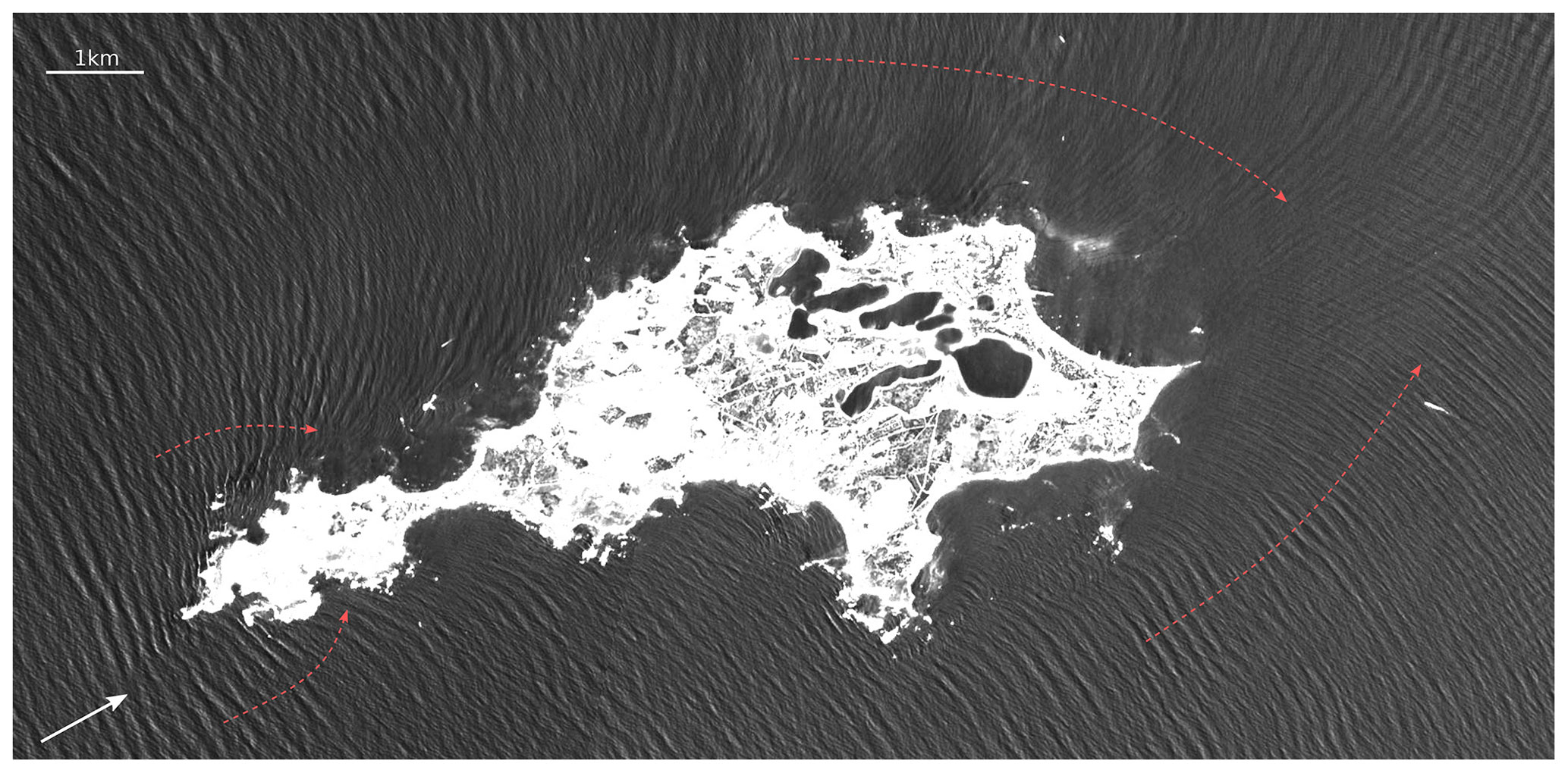
Figure 1Depth refraction of swell against Rottnest Island off the coast of Western Australia depicted by the Copernicus Sentinel-2 mission, processed by ESA, in December 2021. The swell propagates northeastwards (white arrow) and interacts with the bathymetry when coming close to the island. Red arrows indicate the change in wave propagation direction, which is normal to the wave crest. An area subject to crossing waves is found on the east side of the island due to the change in wave propagation direction on both sides of the island.
Recent developments in the ocean modeling community, including assimilation of observations, have led to more realistic ocean-model output fields, which in turn have led to an increased interest in wave–current interaction studies (Babanin et al., 2017). Current-induced refraction has often been singled out as the principal mechanism leading to horizontal wave height variability at scales between 1 km and several hundred kilometers (e.g., Irvine and Tilley, 1988; Ardhuin et al., 2017, 2012). Thus, a number of recent studies employ wave ray equation solvers in order to quantify the impact of refraction (e.g., Romero et al., 2017, 2020; Ardhuin et al., 2012; Masson, 1996; Bôas et al., 2020; Halsne et al., 2022; Saetra et al., 2021; Sun et al., 2022; Gallet and Young, 2014; Rapizo et al., 2014; Kudryavtsev et al., 2017; Bôas and Young, 2020; Jones, 2000; Segtnan, 2014; Mapp et al., 1985; Wang et al., 1994; Liu et al., 1994). However, such implementations are rarely open to the community. To the best of our knowledge, there is no open-source solver available in a high-level computer language to support such analyses. Furthermore, some of the solvers only focus on deep water where the wave ray equations are simplified since the topographic steering is negligible (e.g., Bôas and Young, 2020; Bôas et al., 2020; Mathiesen, 1987; Kenyon, 1971; Rapizo et al., 2014; Kudryavtsev et al., 2017). However, the joint effect of current- and depth-induced refraction at intermediate depth can be important (Romero et al., 2020; Halsne et al., 2022).
The scope of this paper is to present an open-source numerical solver of the wave ray equations implemented in Python. The paper is structured as follows: in Sect. 2 we present the theoretical background for the geometrical optics approximation of the wave ray equations on ambient currents and in variable depths. The numerical discretization and implementation of the equations and model are given in Sect. 3. Furthermore, some ancillary functions that support efficient workflows are also presented in Sect. 3. In Sect. 4, we compare the model output against analytical solutions and inspect the numerical convergence. A selection of examples using the ray tracing module, including idealized current fields and output from ocean circulation models, are presented in Sect. 5. Finally, a brief discussion and some concluding remarks are provided in Sect. 6.
For simplicity, we first derive the wave ray equations in the x direction and then extend the results to both horizontal directions. We assume linear wave theory such that ak≪1, where a denotes the wave amplitude and is the wave number. When considering the kinematics of wave trains through the geometrical optics approximation, it should be emphasized that diffraction is neglected. For a more complete description of the kinematics and dynamics of ocean waves, we refer the reader to Phillips (1977) and Komen et al. (1994).
2.1 The one-dimensional problem
A plane wave propagating in a slowly varying medium is given by
where is the phase function. Here x,t, and δ denote position, time, and the phase, respectively, and σ is the wave angular intrinsic frequency given by the dispersion relation
where d=d(x) is the water depth, which we assume to be constant in time. In the presence of an ambient current , the absolute wave angular frequency is
which is often referred to as the Doppler shift equation. Consider now a phase function in a frame of reference not moving with the current. Since and , by cross-differentiating, we obtain the conservation of wave crests (see Note D, Holthuijsen, 2007, p. 339),
If we also assume local stationarity, i.e., , k becomes constant in time and the frequency remains constant along the rays (). By taking the partial derivative of Eq. (3) while keeping t constant, we obtain
where is the advection velocity, which contains the wave group velocity . We define the material (or total) derivative as
Thus, advection of a wave group is simply
This is the first of the wave ray equations. The evolution of the wave number k follows by inserting Eq. (5) into Eq. (4) such that
which is the second of the wave ray equations. Using the same approach for ω, for a fixed bathymetry we get
which reduces to
for a stationary current , since we consider ambient currents that vary slowly compared to a characteristic wave period. Thus, the absolute wave frequency is constant. Summarized, we have obtained the wave ray equations in one horizontal dimension as
The wave ray equations constitute a set of coupled ordinary differential equations (ODEs) that define a characteristic curve in space and time. They can be solved as an initial value problem if defined with a starting point of and an initial wave period of by using the dispersion relation from Eq. (2). In deep water, where the wavelength , the first term on the right-hand side of Eq. (12) vanishes since tanh (kd)→1 in Eq. (2). Under such conditions the evolution of k is only a function of the horizontal gradients in the ambient current.
2.2 The two-dimensional problem
In 2D we denote the position vector and the ambient current vector . We define the horizontal gradient operator as
where and denote the unit vectors for x and y, respectively. Now, the absolute angular frequency,
and the wave ray equations for a stationary current field become
In the context of spectral wave modeling, the dynamical evolution of the wave field is governed by the wave action balance equation,
Here, is the wave action density, which is a conserved quantity in the presence of currents (Bretherton and Garrett, 1968). The wave action density contains the wave variance density E, which is ∝a2. The right-hand side of Eq. (19) represents sources and sinks of wave action. The wave number gradient operator is
The wave ray equations (Eqs. 16–17) model the terms written (for brevity) with overdots in Eq. (19), i.e.,
There is thus a connection between the wave field dynamics and kinematics where represents the advection of wave action in physical space and represents the refraction (“advection” in k space). The wave action balance (Eq. 19) is solved by third-generation spectral wave models but then discretized either by wave number k or frequency f and direction θ (Komen et al., 1994).
3.1 Finite-difference discretization
The wave ray equations (Eqs. 16–17) are well suited for numerical integration. The ocean_wave_tracing module offers two finite-difference numerical schemes: a fourth-order Runge–Kutta scheme and a forward Euler scheme through its solver method. For readability, the latter is used here to present the discretization of the wave ray equations. The advection (Eq. 16) becomes
Here n denotes the discrete time index, with and . Discrete horizontal indices are given by ; ; and , . The fx is a function of the group velocity and ambient current and becomes (skipping time and horizontal indices for readability)
The evolution in wave number (Eq. 17) becomes
Here, fk is a function of the horizontal derivatives of σ and U. Horizontal derivatives are discretized using a central difference scheme, such that fk becomes
3.2 Stability condition
A constraint for hyperbolic equations in finite-difference numerical schemes is the Courant–Friedrichs–Lewy (CFL) condition, which for a process with advection velocity W demands that the non-dimensional Courant number be defined as
where . If C>1, the process will advect a distance larger than the grid point resolution over a period Δt, leading to instabilities in the numerical solution. A dedicated method, check_CFL, is implemented in the Wave_tracing class and added to the set_initial_condition method (Fig. 2). The Courant number is written to the log file as
The advection velocity (the absolute group velocity as seen from a fixed point) in Eq. (29) is implemented as
which is a good proxy for the magnitude of the maximum advection speed. It may, however, exceed W for n>0 for waves starting in shallow water and propagating towards deeper water. In the check_CFL, .
Algorithm 1Generic workflow code example.
import numpy as npimport maplotlib.pyplot as pltfrom ocean_wave_tracing import Wave_tracing# Defining some properties of the mediumnx = 100; ny = 100 # number of grid points in x- and y-directionx = np.linspace(0,2000,nx) # size x-domain [m]y = np.linspace(0,3500,ny) # size y-domain [m]T = 250 # simulation time [s]U=np.zeros((nx,ny))U[nx//2:,:]=1# Define a wave tracing objectwt = Wave_tracing(U=U,V=np.zeros((ny,nx)),nx=nx, ny=ny, nt=150,T=T,dx=x[1]-x[0],dy=y[1]-y[0],nb_wave_rays=20,domain_X0=x[0], domain_XN=x[-1],domain_Y0=y[0], domain_YN=y[-1],)# Set initial conditionswt.set_initial_condition(wave_period=10,theta0=np.pi/8)# Solvewt.solve()3.3 Model simulation workflow
The wave ray equations are implemented in Python 3 in the ocean_wave_tracing module available on GitHub at https://github.com/hevgyrt/ocean_wave_tracing (last access: 6 November 2023) under a GPL v.3 license. It is based on common native Python libraries and open-source projects. Key open-source projects include numpy (numerical Python – https://numpy.org/, last access: 6 November 2023), matplotlib (https://matplotlib.org/, last access: 6 November 2023), and xarray (https://docs.xarray.dev/en/stable/, last access: 6 November 2023). The latter library is a large project, which has become a de facto standard in geophysical sciences for analyzing and dealing with multi-dimensional data. The wave ray tracing tool is a class instance, and the Wave_tracing object contains multiple auxiliary methods before and after performing the numerical integration. Here, we will focus on the workflow, input fields, implementation, and the ancillary methods enclosing the wave ray tracing solver method.
3.3.1 Operating conditions
A set of fixed conditions are specified for the ocean_wave_tracing module. The most important conditions include the following:
-
The model domain must be rectangular and in Cartesian coordinates with a uniform horizontal resolution in each direction.
-
Units must follow the SI system with length scale units of meters (m) and seconds (s). The angular units are radians (rad). Wave propagation direction θ follows a right handed coordinate system with θ=0 being parallel to the x axis and propagating in the positive x direction.
-
Variable names, structures, and metadata are, to a large extent, based on the Climate and Forecast (CF) metadata convention (https://cfconventions.org/, last access: 6 November 2023).
3.3.2 Ray tracing model initialization
A flowchart of the model simulation workflow is given in Fig. 2 and an associated code example in Alg. 1. Firstly, a wave ray tracing object Wave_tracing is initialized by an __init__ method. The input variables define the ambient conditions and include
-
the ambient current U,V = U;
-
the bathymetry depth (optional);
-
the boundaries X0,XN,Y0, and YN and horizontal resolution dx and dy of the domain;
-
the number of time steps nt and total duration time for wave propagation T;
-
the number of wave rays nb_wave_rays.
The current is allowed to vary in time by setting temporal_evolution=True, but it is up to the user to make sure that U(t,x) is not violating Eq. (18) by . If the bathymetry is not specified, the model assumes deep-water waves and sets a fixed uniform depth at 105 m. Depth values are defined as positive, implying that negative values will be treated as land if both negative and positive values are present through a dedicated bathymetry checker (check_bathymetry), which is invoked within __init__. Furthermore, the input velocity field is checked and xarray datasets are created for the bathymetry and velocity field as class variables following the CF convention.
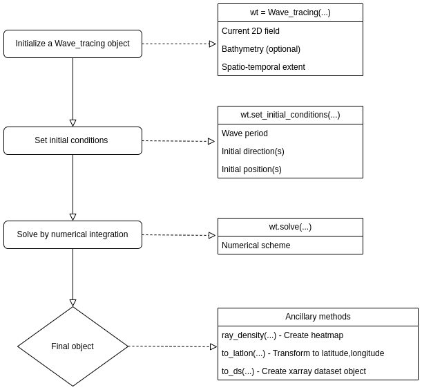
Figure 2Flowchart of the workflow from initializing a ray tracing object to solving the wave ray tracing equations. The left column denotes the most important steps in the workflow, and the right column highlights the most important parameters and supporting methods under each step.
3.3.3 Setting the initial conditions
Before the numerical integration, initial conditions for the ODEs are specified in a dedicated set_initial_condition() method (Alg. 1, Fig. 2). Here the initial wave period Tn=0, wave propagation direction , and initial position are specified. By utilizing the rectangular model domain, the initial position can most easily be given as one of the sides of the domain, i.e., top, bottom, left, or right, where left is default (see Alg. 1). In such cases, the number of wave rays is spread uniformly on the selected boundary. Another option is to specify initial grid points ipx and ipy for each wave ray. Similarly, can also be specified for each ray, or a single uniform direction can be given for all rays. Such examples are provided later.
The model is solved for a single wave frequency, dictated by the initial wave period Tn=0. The wave number k is retrieved from Tn=0 using Eq. (2), which in intermediate depths requires an iterative solver. Using the approximation by Eckart (1952), the error in k is less than 5 % (Holthuijsen, 2007).
3.3.4 Numerical integration
Numerical integration of Eqs. (23)–(28) is initiated by invoking the solver method. Here, ∇hU is computed prior to the integration using the numpy gradient method. The integration is performed iteratively in a Lagrangian sense by computing the next position rn+1 from the current position rn for each wave ray. Thus, the solver keeps track of the horizontal indices l and j for every time step and for each wave ray in the model domain. Hence, the numerical integration for the wave rays can follow a vectorized approach, which is conceptually visualized in Fig. 3. For a given position r, the properties of the ambient medium, i.e., the current and bathymetry, are selected using a nearest-neighbor approach.
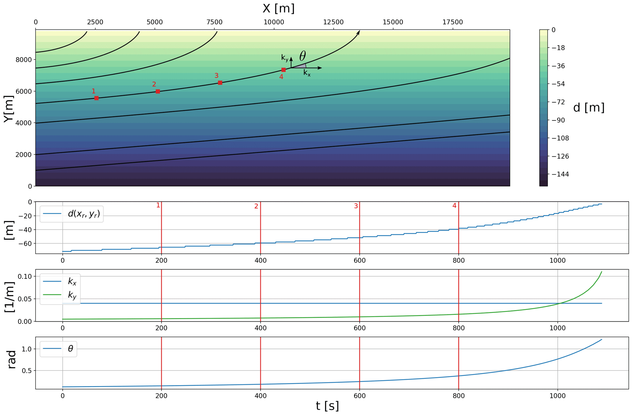
Figure 3A conceptual figure highlighting the workflow strategy of the model. Here, depth refraction of a T=10 s period wave propagating from left with an initial angle rad is shown for seven different rays (black lines). The propagation path for each wave ray is computed simultaneously through vectorization. The lower panels denote the change in depth, evolution in k, and corresponding wave propagation direction, θ, in time along one of the rays. As expected, the wave rays deflect towards shallower regions due to the increase in the ky wave number component.
Even though ∇hU is static for each model field, ∇hσ in Eq. (28) must be computed for each iteration n since the wave number k evolves in time. Furthermore, for each iteration of n, the wave propagation direction θn is computed from kn using the numpy atan2 function.
After a successful call of the solve() function, the Wave_tracing object will have populated its class variables for the wave rays being (ray_x,ray_y), (ray_kx,ray_ky), ray_k, ray_theta, ray_cg, and (ray_U,ray_V), which are the horizontal position vector, wave number vector, wave number, wave propagation direction, wave group velocity, and ambient current vector, respectively. All of the aforementioned class variables have the dimensions number_of_wave_rays×N.
The numerical scheme used in the solver method is configurable by the user, and the default is a fourth-order Runge–Kutta scheme. That is, the numerical scheme is generic and detached from the wave ray equations. The schemes are available in a separate utility function util_solvers, which contains (currently two) numerical schemes which are defined Python classes in a hierarchy with a generic ODE solver as the top node. That is, each sub-class has its own advance method, which corresponds to the numerical scheme. This approach is to a large extent built on material from Langtangen (2016). Furthermore, the util_solvers also contain the advection and wave number evolution functions in Eq. (25) and Eq. (28), respectively.
3.4 Ancillary methods and testing
3.4.1 Ancillary functions
Ancillary functions include methods which are considered useful for the user community. The current version has four methods, three within the Wave_tracing object and one outside the object.
The method outside the Wave_tracing object is targeted for data preparation before model initialization. It is not strictly a Python method, but it is a generic workflow for data retrieval. More specifically, since the ray tracing model is focused on ocean currents and bathymetry, it is natural to exploit variable fields from ocean circulation models. It is common for oceanographic centers to disseminate model results under a free and open data policy and to enable the Open-source Project for a Network Data Access Protocol (OPeNDAP – https://www.opendap.org/, last access: 6 November 2023) on the data distribution server (e.g., THREDDS – https://www.unidata.ucar.edu/software/tds/current/, last access: 6 November 2023 or HYRAX – https://www.opendap.org/software/hyrax-data-server, last access: 6 November 2023). The OPeNDAP enables spatio-temporal subsetting to be carried out on the server side and thus avoids the problem of downloading huge amounts of data prior to use. Such user-defined subsets can be accessed directly via data streaming by using common netCDF4 readers (https://www.unidata.ucar.edu/software/netcdf/, last access: 6 November 2023), which are available in xarray. The ancillary method, or workflow, is provided in the Jupyter notebook extract_ocean_model_data.ipynb. Here, the user can plot and check the user-defined area and temporal extent prior to writing the subset to disk or initiating the Wave_tracing object directly. It is common for ocean circulation models to have output variable fields with hourly temporal resolution such that U(t,x) is unlikely to violate Eq. (18). However, it is up to the user to understand the limitations of the model if simulating wave rays for very long shallow-water waves like tsunamis and tidal waves.
The first of the three class methods within the Wave_tracing object is a transformation method from projection coordinates to latitude and longitude values, which is called to_latlon() (see Fig. 2). That is, when using ocean-circulation-model field variables as input data, it is not readily possible to compare the Wave_tracing output with other sources of data since ocean-model field variables are most often in a specific projection. In this context, using latitude and longitude coordinates is often much more convenient. The method requires the proj4 string of the ocean-model domain and performs coordinate transformation using the pyproj (https://pyproj4.github.io/pyproj/stable/, last access: 6 November 2023) library in Python. Even if not required, it is common that the proj4 string is listed in the grid_mapping variable in a CF-compliant ocean-model dataset.
The second ancillary function is based on the wave ray density method by Rapizo et al. (2014) and is called ray_density(). It computes the relative number of wave rays within user-defined grid boxes, which can be considered proportional to the wave height and thus the horizontal wave height variability. The method returns a 2D grid and the associated ray density variable.
The third method takes care of converting all the characteristic Wave_tracing class variables into an xarray dataset, including latitude and longitude if the proj4 string is given as input. The method is called to_ds(). The output xarray dataset follows the CF convention for metadata. Thus, the data can utilize all the functionality within xarray, including the plotting and writing of data to disk. Examples using all the methods listed above will be shown later in Sect. 5.
3.4.2 Tests
The ocean_wave_tracing repository is equipped with unit tests written in the framework of Pythons pytest. Unit tests are tailored for the methods within and used by the Wave_tracing class and typically check the numerical implementation against known solutions. For instance, the computation of wave celerity for deep and shallow water is tested against analytical solutions.
For integration tests, a set of example scripts running the entire chain of operations is embedded in the test folder. Such tests are also implicitly inherent in the scripts provided in the notebooks and verification folders, since these notebooks run the entire chain. Moreover, continuous integration tests are embedded in the repository utilizing the poetry project (https://python-poetry.org/, last access: 6 November 2023).
Here we verify the output of the Wave_tracing solver against analytical solutions for idealized cases for depth- and current-induced refraction. Model differences are given as the absolute relative difference between the analytical solution A and the numerical model solution B for an arbitrary variable z as
given in the units of percentage.
4.1 Snell's law
When only considering the bathymetry, Snell's law,
applies for parallel depth contours (see Note 7A, Holthuijsen, 2007, p. 207). Here, subscripts 1 and 2 indicate the properties of the wave and medium before and after being transmitted through an interface, which here are lines of different bathymetry, and c is the phase speed. The ϕ1 denotes the incidence angle between the wave ray and the normal to the interface, and ϕ2 is the angle of refraction after the interaction.
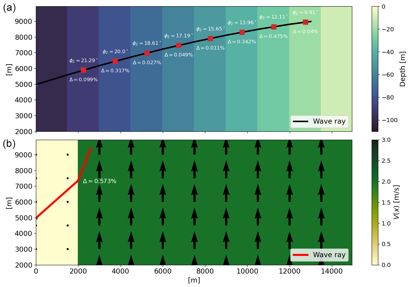
In the presence of ambient currents, Snell's law can be written for a horizontally sheared current V=V(x) (Kenyon, 1971),
Verification of the wave ray tracing model results against Eqs. (33) and (34) is shown in the upper and lower panels of Fig. 4, respectively. For the idealized bathymetry, the wave ray tracing was performed for a shallow-water wave with wavelength λ=10 000 m propagating towards a stepwise shallower region.
Here, Δϕ2 was computed for each new depth regime (upper panel Fig. 4a). For the horizontally sheared current (Fig. 4b), a T=10 s period deep-water wave propagated through the current field where
The relative differences in both the idealized bathymetry and horizontally sheared current cases listed above were (Fig. 4). The script producing Fig. 4 and computing the analytical results is available as a Jupyter notebook under verification/snells_law.ipynb.
4.2 Wave deflection
For deep-water waves, there is a direct relation between wave ray curvature and the vertical vorticity (henceforth vorticity) (Kenyon, 1971; Dysthe, 2001):
valid for . Here, positive vorticity will deflect a wave to the left relative to its wave propagation direction and to the right for negative vorticity. The ratio with the wave group velocity also entails that shorter waves will deflect more compared with longer waves.
An approximate wave deflection angle can be computed from Eq. (36) by adding a characteristic ζ=ζ0 and length scale l such that (Gallet and Young, 2014)
We use the idealized horizontally sheared current,
where α increases linearly from α=0 at y=0 to at y=Y such that ζ values are constant within the regions. An assessment of θν for a T=10 s period deep-water wave propagated through Eq. (38) is shown in Fig. 5. Here, the solution in the lower panel also uses Eq. (38) but with a minus sign in front of α. Relative differences between the model and analytical solution are Δ(θν)∼100 %. The difference is a sum of the numerical errors together with the approximate equality in Eq. (37). Furthermore, the difference between the simulation of the negative and positive vorticity ζ is also due to the advection of the current. Furthermore, the deflection direction for negative and positive ζ is readily seen in Fig. 5. The full analysis is available in the verification/wave_deflection.ipynb notebook in the GitHub repository.
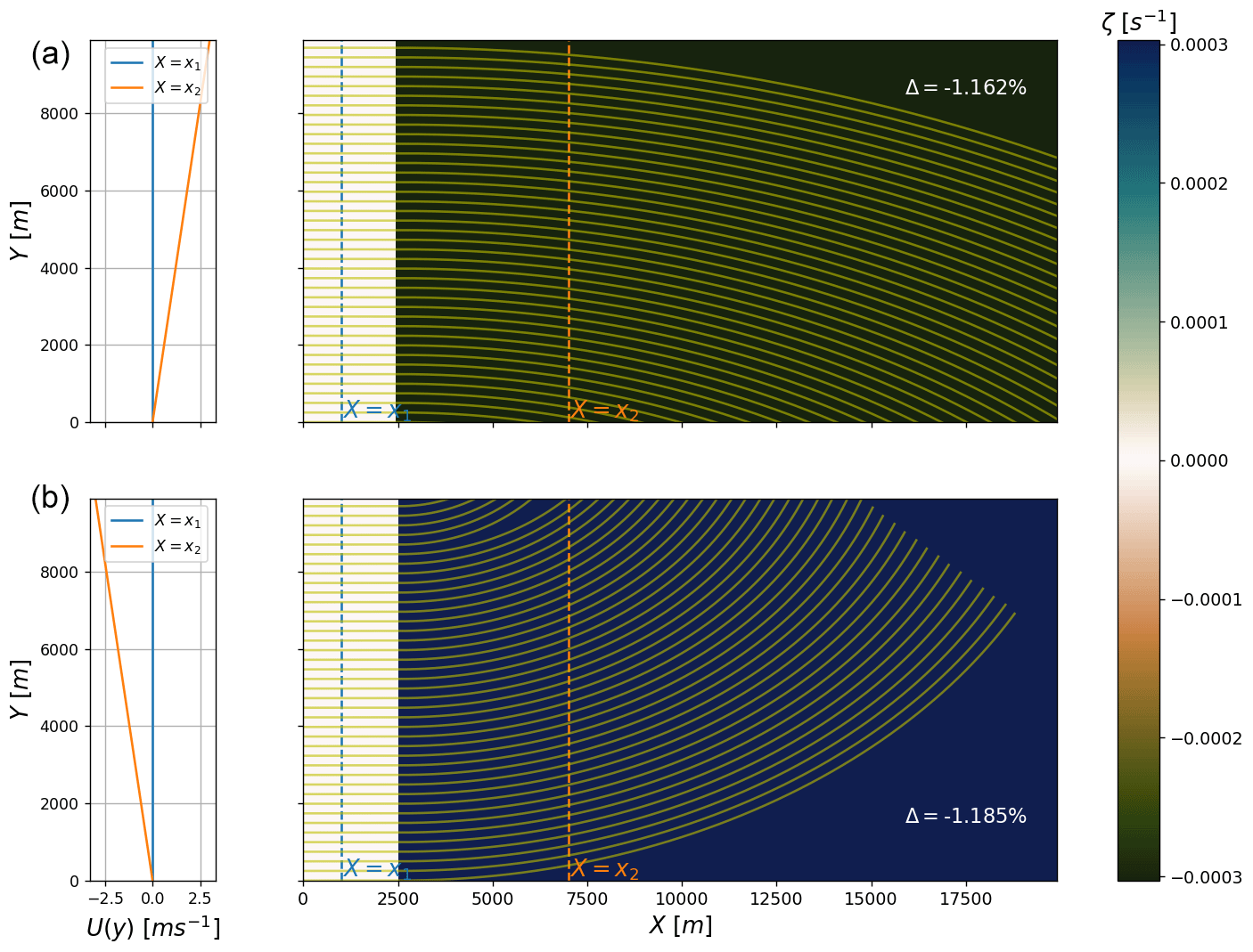
Figure 5Verifying the approximate solutions of wave deflection (Eq. 37) against the wave ray tracing output for cases with idealized negative (a) and positive vorticity ζ (b). The associated velocity field at is given in the left column plots. The relative differences Δθν [Eq. 32] using l=2500 m are given for both cases (see insert text). Yellow lines denote the wave rays.
4.3 Numerical convergence
The numerical convergence for decreasing values of the CFL number C is tested for the conservation of absolute frequency ω in Eq. (18). For the idealized case of a deep-water wave propagating in the x direction from a region with U=0 to a region with an opposing current , Eq. (18) requires
where subscript 0 denotes the region with U=0. For deep water, the phase speed such that Eq. (39) can be rearranged and
In our example, k=0.046 m−1 for a T=10 s period wave propagating into the region . The numerical convergence for Eq. (18) is shown in Fig. 6. Here, the error Δω decreases with decreasing C due to the increasing number of time steps N. The error does not decrease monotonically, however, since k must be solved sufficiently many times within the region where to obtain its correct value. Nevertheless, the solution converges to the analytical solution with decreasing C (see kan in Fig. 6). The test on the numerical convergence is available in the GitHub repository in the verification/numerical_convergence_ omega.ipynb notebook.
Here we provide some use examples of the wave ray tracing model, which include simulations under idealized current and bathymetry fields and ambient conditions retrieved from an ocean circulation model. The code for running the tool is similar to the generic example given in Alg. 1 but with different ambient and initial conditions. The idealized current fields are part of the repository as a netCDF4 file and reproducible in the notebooks/create_idealized_current_and_ bathymetry.ipynb notebook. The examples include specifying different initial conditions as well as utilizing the ancillary functions described in Sect. 3.4.1.
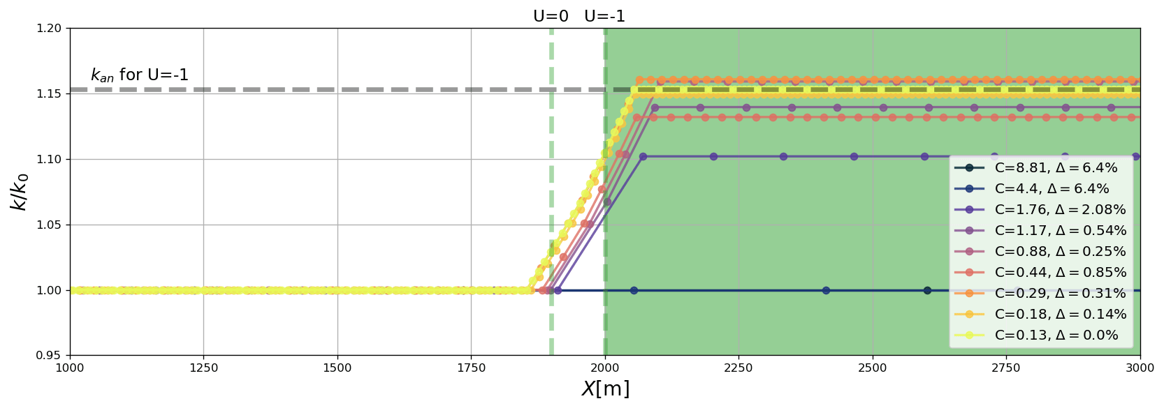
Figure 6The numerical convergence tested for conservation of absolute frequency ω in Eq. (18). The convergence is tested for an increasing number of discrete time indices n with an accompanied decreasing Courant number C. Here, a domain with velocity field U=0 for X<2000 and for X≧2000, where ΔX=100 m (see dashed vertical lines), was used. The analytical value kan is obtained from Eq. (40). The relative error decreases with C. The results here are obtained by using the RK4 scheme, but similar results are obtained using the FE (not shown).
5.1 Idealized cases
Cases with depth-induced refraction are shown in Fig. 7. Here the idealized cases show the expected veering of wave rays towards shallower regions when the deep-water limit is no longer applicable. The examples also show how the initial position rn=0 can be set differently using the different sides of the domain (i.e., left and bottom in Fig. 7a, c, d) and from a single point with the initial propagation angle uniformly distributed in a sector (Fig. 7b).
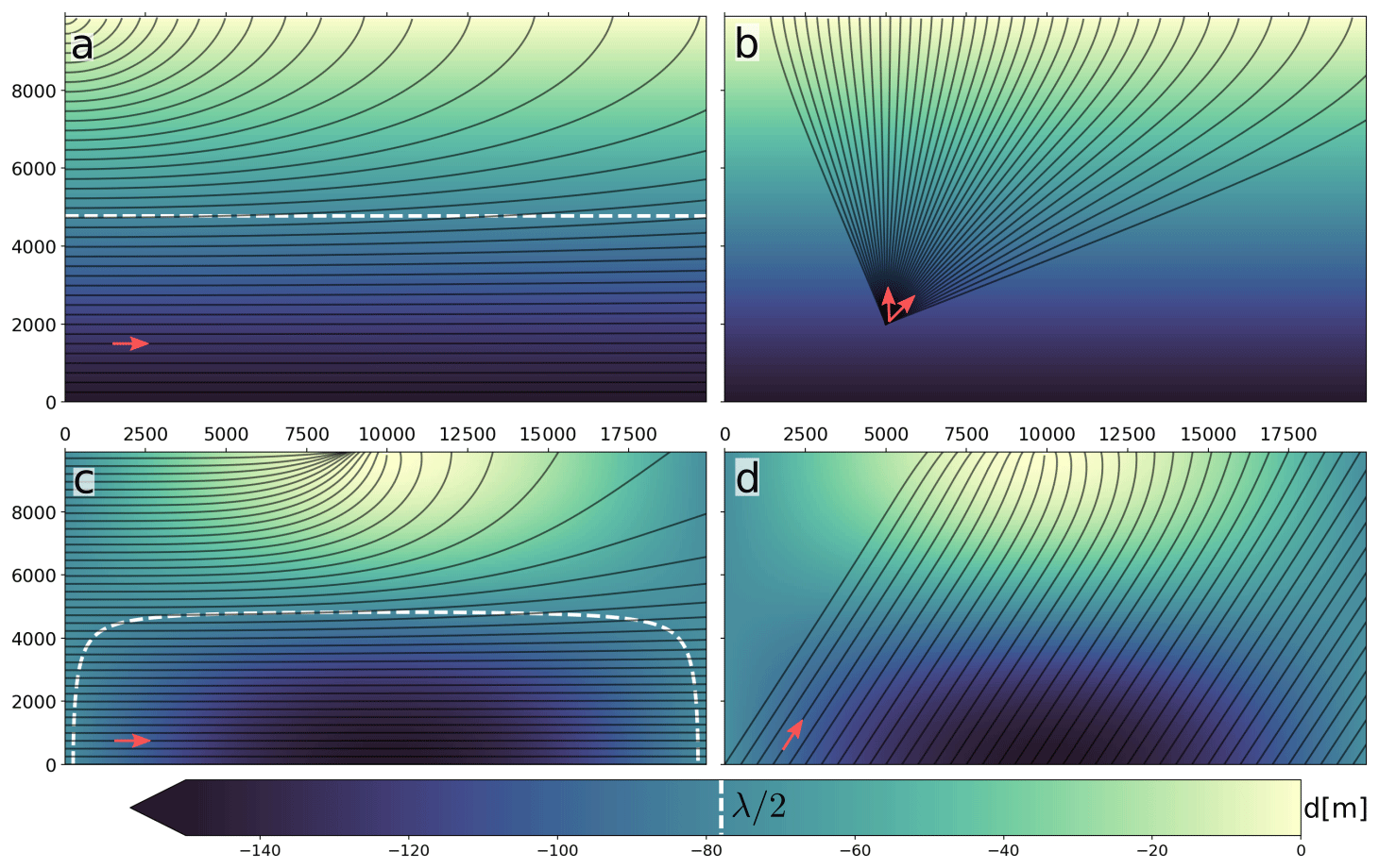
Figure 7Examples of depth refraction of a long crested 10 s period wave using various initial positions and initial propagation directions (red arrows), for two different depth profiles in the upper (a, b) and lower panels (c, d). Waves with (λ=156 m on deep water, white contour lines) will not “feel” the bottom and thus not be refracted.
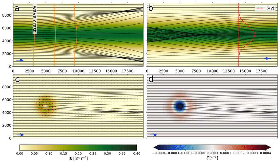
Figure 8Examples of current-induced refraction under different flow regimes and initial propagation directions (blue lines). Panel (a) denotes the evolution of the wave crest (orange lines) as it rides along a current jet (see current profile U(y) in b). In panel (b) the current jet is opposing the waves, inducing focal points in the middle of the jet. Panel (c) shows how a characteristic current whirl impacts the wave propagation paths, and (d) denotes the relation between deflection angle and the vorticity, ζ.
Cases with current-induced refraction in deep water are shown in Fig. 8. Examples of wave trains both following and opposing a horizontally sheared current are provided (Fig. 8a, b). The ambient current causes areas of converging and crossing wave rays, which are known as caustics or focal points. Furthermore, an example of waves propagating through an idealized oceanic eddy is shown (Figs. 8c, d).
The joint effect of current- and depth-induced refraction at intermediate depth is shown in Fig. 9. Here, the ray_density method is used to highlight the different focal points obtained in deep water and when the waves are also influenced by the bathymetry.
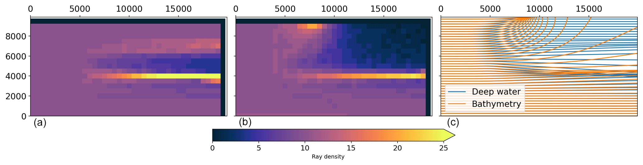
Figure 9The impact of depth and current refraction on horizontal wave height variability as seen through wave ray density plots. Panel (a) shows results using the wave ray density method for a current whirl on deep water (see Fig. 8c). Panel (b) shows the impact on wave ray density for the same current whirl but on intermediate depths, i.e., adding the bathymetry in Fig. 7c. Panel (c) denotes the difference in the wave ray paths between the two cases.
All the examples listed above are available in the notebooks/idealized_examples.ipynb notebook.
5.2 Ocean-model output
Examples of using surface currents and bathymetry extracted from the operational coastal ocean circulation model at the Norwegian Meteorological Institute (Albretsen et al., 2011) as input in wave tracing simulations are shown for different regions in Fig. 10. Here, the to_latlon() method has been used together with to_ds() in order to visualize the output on a georeferenced map. Figure 10b denotes the refraction due to currents and bathymetry (red rays), compared with bathymetry only (yellow rays). There are clear differences between the wave rays with and without currents. The current field used here spanned four model output time steps with an hourly temporal resolution. Figure 10c and d show how the wave kinematics are affected by a barotropic tidal current under two characteristic cycles. In the lower left panel, the tidal current gives rise to a focal point and crossing wave rays. Cases similar to the latter two were investigated in Halsne et al. (2022), comparing the results with output from a spectral wave model (Eq. 19). The examples provided here are available in the notebooks/ocean_model_example.ipynb notebook.
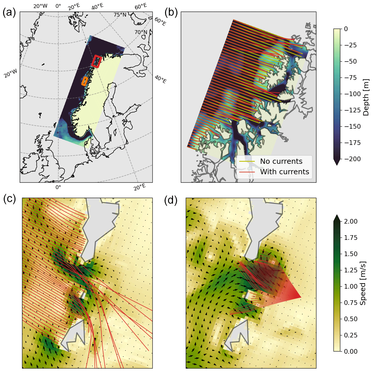
Figure 10The impact of currents and bathymetry on wave propagation paths using current and bathymetry fields from an 800 m resolution Regional Ocean Modeling System (ROMS) model in Northern Norway (a). (b) Subset in the red rectangle in (a); it shows how time-varying surface currents (i.e., four model time steps) impact the wave propagation paths for a T=10 s period wave (red rays) when compared to refraction due to bathymetry only (yellow rays). (c, d) Subset in the orange rectangle in (a); panels (c) and (d) show the impact of a tidal current on the wave propagation paths for a T=10 s period wave (c) and a T=7 s period wave (d). Here, arrows denote the direction of the ambient current.
The famous textbook example of trapped waves in the Agulhas Current east of South Africa is shown in Fig. 11. Here, the wave tracing simulations used the surface current from the ESA's GlobCurrent project (https://data.marine.copernicus.eu/product/MULTIOBS_GLO_PHY_REP_015_004/description, last access: 6 November 2023). The particular point in time for the simulation is the same as used in Kudryavtsev et al. (2017) (i.e., 4 January 2016, see their Figs. 14–15) but here with an apparently coarser horizontal resolution in the current forcing.
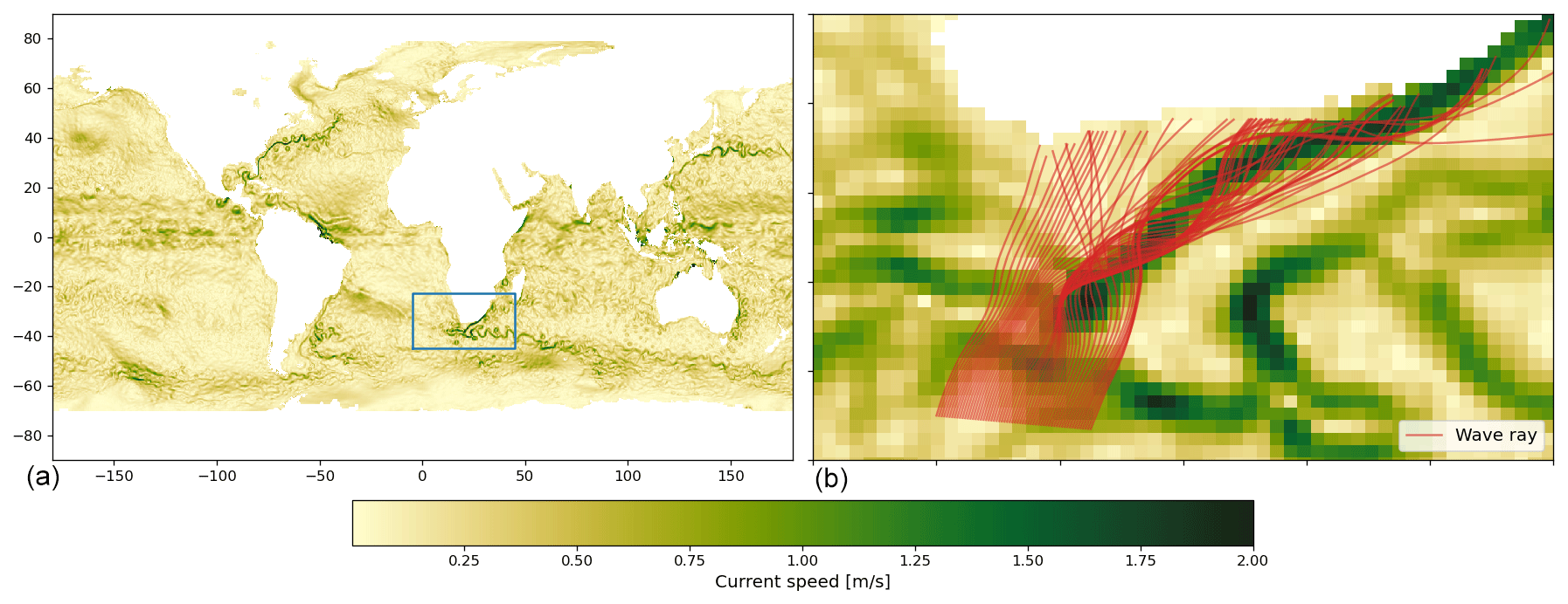
Figure 11Focusing of wave rays by the Agulhas Current. Here, surface current data from the GlobCurrent project are used from 4 January 2016 (a). The data are originally given in spherical latitude and longitude coordinates but are approximated here in the area of interest to equidistant Cartesian coordinates with 22 and 28 km spatial resolution in the x and y directions, respectively. The famous trapping of wave rays within the branch of the Agulhas Current is shown in (b) using a T=10 s period wave. The duration of the run was 62 h, and 18 consecutive model output times (temporal resolution of 3 h) were used.
We have presented a Python-based, open-source, finite-difference ray tracing model for arbitrary depths at variable currents. The Wave_tracing module has been tested and verified against analytical solutions and tested for numerical convergence. The solver comes with a set of ancillary functions aimed at supporting relevant workflows for data retrieval, transformation, and visualization in the scientific community as well as being compatible with the standardized Climate and Forecast (CF) metadata conventions. Such workflows have been documented and are available in the repository as examples for the end users.
To the best of our knowledge, no such modeling tool is openly available in a high-level computing language despite its usefulness for the investigation and quantification of the impact of ambient currents and bathymetry on the wave field (e.g., Romero et al., 2017, 2020; Ardhuin et al., 2012; Masson, 1996; Bôas et al., 2020; Halsne et al., 2022; Saetra et al., 2021; Sun et al., 2022; Gallet and Young, 2014; Rapizo et al., 2014; Kudryavtsev et al., 2017; Bôas and Young, 2020).
The solver is applicable to waves in finite depth, which is in contrast to previously reported models which handle only current-induced refraction in deep water (e.g., Bôas and Young, 2020; Bôas et al., 2020; Mathiesen, 1987; Kenyon, 1971; Rapizo et al., 2014; Kudryavtsev et al., 2017). For intermediate depths, the joint effect of current- and depth-induced refraction can be very important for the wave height variability (Fig. 9). Such examples were presented in Halsne et al. (2022) and Romero et al. (2020), where the combined refraction of wave rays due to the ambient current and bathymetry caused focusing, which led to a significant increase in the local wave height (see Fig. 11 in Halsne et al., 2022 and Fig. 14 in Romero et al., 2020).
The effect of vertically sheared currents is usually neglected in coupled wave model simulations since it is a second-order effect. However, in strong baroclinic environments, such shear may strongly affect the absolute angular frequency (Zippel and Thomson, 2017). In ocean_wave_tracing, the impact of vertically sheared currents can be accounted for by computing an effective depth-integrated current (e.g., Kirby and Chen, 1989). Such an extension is easy to add as an optional method in the ray tracing model initialization due to the class structure (see Sect. 3.3.2), given that the input ambient current field is three-dimensional. However, and as shown by Calvino et al. (2022), care should be taken since numerical errors can be introduced in the computation of an effective current from horizontally varying 3D sheared currents with coarse vertical resolution. An implementation of the effective current is planned as a future extension in ocean_wave_tracing.
The ocean_wave_tracing module does not support wave reflection. Such processes are complex but could be added later. This means that wave rays can essentially propagate through land and out of the model domain. Such effects are, however, circumvented by using numpy's masked arrays and not-a-number (NaN) values. For instance in the bathymetry_checker, negative bathymetry values will be treated as land and set to a numpy NaN. When plotting, NaN values do not appear. Furthermore, masked values are often standard in ocean circulation models, and thus wave rays “stop” when entering land grid points (see Fig. 10).
Solving the ray equation using a high-level language such as Python gives added execution time and memory usage compared to lower-level languages. However, execution times are normally on the order of 101 s but will obviously increase with the number of time steps nt. It is possible to further speed up the code by utilizing other modules and by making the code base more dense in terms of reducing the amount of code. However, the objective of the wave ray tracing tool described here is neither to create a substitute to wave models nor to optimize it for large and/or long simulations. It is rather to provide a framework that is easy to understand and simple to run. In addition, a comprehensible code base makes the tool suitable for further development by other contributors. Furthermore, best practices like vectorization have been used in order to speed up the solver, without loss of general readability of the code.
The source code is available at https://github.com/hevgyrt/ocean_wave_tracing (last access: 6 November 2023) under a GPL v.3 license with DOI https://doi.org/10.5281/zenodo.7602540 (Halsne et al., 2023). ROMS data from MET Norway is available on under a free an open data policy at https://thredds.met.no/thredds/fou-hi/norkyst800v2.html?dataset=norkyst800m_1h_be (Albretsen et al., 2011). This study has been conducted using E.U. Copernicus Marine Service Information, specifically using the ESA GlobCurrent dataset; https://doi.org/10.48670/moi-00050 (GlobCurrent E.U. Copernicus Marine Service Information, 2022).
The supplement related to this article is available online at: https://doi.org/10.5194/gmd-16-6515-2023-supplement.
TH designed and implemented the software, including the formal analysis and model validation, and wrote the manuscript draft. GH supported the development and GitHub integration. GH, KHC, and ØB reviewed and edited the manuscript.
The contact author has declared that none of the authors has any competing interests.
Publisher’s note: Copernicus Publications remains neutral with regard to jurisdictional claims made in the text, published maps, institutional affiliations, or any other geographical representation in this paper. While Copernicus Publications makes every effort to include appropriate place names, the final responsibility lies with the authors.
This research was partly funded by the Research Council of Norway through the project MATNOC (grant no. 308796). Trygve Halsne and Øyvind Breivik are grateful for additional support from the Research Council of Norway through the StormRisk project (grant no. 300608).
This research has been supported by the Norges Forskningsråd (grant nos. MATNOC 308796 and Stormrisk 300608).
This paper was edited by P. N. Vinayachandran and reviewed by Leonel Romero and one anonymous referee.
Albretsen, J., Sperrevik, A. K., Staalstrøm, A., Sandvik, A. D., Vikebø, F., and Asplin, L.: NorKyst-800 report no. 1: User manual and technical descriptions, Tech. Rep. 2, Institute of Marine Research, Bergen, Norway, https://www.hi.no/en/hi/nettrapporter/fisken-og-havet/2011/fh_2-2011_til_web (last access: 6 November 2023), 2011. a, b
Ardhuin, F., Roland, A., Dumas, F., Bennis, A.-C., Sentchev, A., Forget, P., Wolf, J., Girard, F., Osuna, P., and Benoit, M.: Numerical Wave Modeling in Conditions with Strong Currents: Dissipation, Refraction, and Relative Wind, J. Phys. Oceanogr., 42, 2101–2120, https://doi.org/10.1175/JPO-D-11-0220.1, 2012. a, b, c
Ardhuin, F., Gille, S. T., Menemenlis, D., Rocha, C. B., Rascle, N., Chapron, B., Gula, J., and Molemaker, J.: Small-scale open ocean currents have large effects on wind wave heights, J. Geophys. Res.-Oceans, 122, 4500–4517, https://doi.org/10.1002/2016JC012413, 2017. a
Babanin, A. V., van der Weshuijsen, A., Chalikov, D., and Rogers, W. E.: Advanced wave modeling, including wave-current interaction, J. Mar. Res., 75, 239–262, https://doi.org/10.1357/002224017821836798, 2017. a
Bretherton, F. P. and Garrett, C. J. R.: Wavetrains in Inhomogeneous Moving Media, P. Roy. Soc. Lond. A Mat., 302, 529–554, ISSN 0080-4630, 1968. a
Bôas, A. B. V. and Young, W. R.: Directional diffusion of surface gravity wave action by ocean macroturbulence, J. Fluid Mech., 890, 1469–7645, https://doi.org/10.1017/jfm.2020.116, 2020. a, b, c, d
Bôas, A. B. V., Cornuelle, B. D., Mazloff, M. R., Gille, S. T., and Ardhuin, F.: Wave-Current Interactions at Meso- and Submesoscales: Insights from Idealized Numerical Simulations, J. Phys. Oceanogr., 50, 3483–3500, https://doi.org/10.1175/JPO-D-20-0151.1, 2020. a, b, c, d
Calvino, C., Dabrowski, T., and Dias, F.: Theoretical and applied considerations in depth-integrated currents for third-generation wave models, AIP Adv., 12, 015017, https://doi.org/10.1063/5.0077871, 2022. a
Dysthe, K. B.: Refraction of gravity waves by weak current gradients, J. Fluid Mech., 442, 157–159, https://doi.org/10.1017/S0022112001005237, 2001. a
Eckart, C.: The propagation of gravity waves from deep to shallow water, https://ui.adsabs.harvard.edu/abs/1952grwa.conf..165E (last access: 6 November 2023), U. S. National Bureau of Standards, 1952. a
Gallet, B. and Young, W. R.: Refraction of swell by surface currents, J. Mar. Res., 72, 105–126, https://doi.org/10.1357/002224014813758959, 2014. a, b, c
GlobCurrent E.U. Copernicus Marine Service Information (CMEMS): Global Total Surface and 15m Current (COPERNICUS-GLOBCURRENT) from Altimetric Geostrophic Current and Modeled Ekman Current Reprocessing, Marine Data Store (MDS) [data set], https://doi.org/10.48670/moi-00050, 2022. a
Halsne, T., Bohlinger, P., Christensen, K. H., Carrasco, A., and Breivik, Ø.: Resolving regions known for intense wave–current interaction using spectral wave models: A case study in the energetic flow fields of Northern Norway, Ocean Model., 176, 102071, https://doi.org/10.1016/j.ocemod.2022.102071, 2022. a, b, c, d, e, f
Halsne, T., Christensen, K. H., Hope, G., and Breivik, Ø.: Model repository, Zenodo [code], https://doi.org/10.5281/zenodo.7602540, 2023. a
Holthuijsen, L. H.: Waves in Oceanic and Coastal Waters, Cambridge University Press, https://doi.org/10.1017/CBO9780511618536, 2007. a, b, c, d
Irvine, D. E. and Tilley, D. G.: Ocean wave directional spectra and wave-current interaction in the Agulhas from the Shuttle Imaging Radar-B synthetic aperture radar, J. Geophys. Res.-Oceans, 93, 15389–15401, https://doi.org/10.1029/JC093iC12p15389, 1988. a
Johnson, J. W.: The refraction of surface waves by currents, Eos, Transactions American Geophysical Union, 28, 867–874, https://doi.org/10.1029/TR028i006p00867, 1947. a
Jones, B.: A Numerical Study of Wave Refraction in Shallow Tidal Waters, Estuar. Coast. Shelf Sci., 51, 331–347, https://doi.org/10.1006/ecss.2000.0679, 2000. a
Kenyon, K. E.: Wave refraction in ocean currents, Deep-Sea Res., 18, 1023–1034, https://doi.org/10.1016/0011-7471(71)90006-4, 1971. a, b, c, d, e, f
Kirby, J. T. and Chen, T.-M.: Surface waves on vertically sheared flows: Approximate dispersion relations, J. Geophys. Res.-Oceans, 94, 1013–1027, https://doi.org/10.1029/JC094iC01p01013, 1989. a
Komen, G. J., Cavaleri, L., Doneland, M., Hasselmann, K., Hasselmann, S., and Janssen, P. A. E. M. (Eds.): Dynamics and Modelling of Ocean Waves, Cambridge Univeristy Press, https://doi.org/10.1017/CBO9780511628955, 1994. a, b
Kudryavtsev, V., Yurovskaya, M., Chapron, B., Collard, F., and Donlon, C.: Sun glitter imagery of surface waves. Part 2: Waves transformation on ocean currents, J. Geophys. Res.-Oceans, 122, 1384–1399, 2017. a, b, c, d, e
Langtangen, H. P.: A Primer on Scientific Programming with Python, vol. 6 of Texts in Computational Science and Engineering, Springer, Berlin, Heidelberg, ISBN 978-3-662-49886-6 978-3-662-49887-3, https://doi.org/10.1007/978-3-662-49887-3, 2016. a
Liu, A. K., Peng, C. Y., and Schumacher, J. D.: Wave-current interaction study in the Gulf of Alaska for detection of eddies by synthetic aperture radar, J. Geophys. Res.-Oceans, 99, 10075–10085, https://doi.org/10.1029/94JC00422, 1994. a
Mapp, G. R., Welch, C. S., and Munday, J. C.: Wave refraction by warm core rings, J. Geophys. Res., 90, 7153, https://doi.org/10.1029/JC090iC04p07153, 1985. a
Masson, D.: A Case Study of Wave–Current Interaction in a Strong Tidal Current, J. Phys. Oceanogr., 26, 359–372, https://doi.org/10.1175/1520-0485(1996)026<0359:ACSOWI>2.0.CO;2, 1996. a, b
Mathiesen, M.: Wave refraction by a current whirl, J. Geophys. Res.-Oceans, 92, 3905–3912, https://doi.org/10.1029/JC092iC04p03905, 1987. a, b, c
Phillips, O. M.: The Dynamics of the Upper Ocean, Cambridge University Press, Cambridge, 2 edn., https://doi.org/10.1002/zamm.19790590714, 1977. a
Rapizo, H., Babanin, A., Gramstad, O., and Ghantous, M.: Wave Refraction on Southern Ocean Eddies, in: 19th Australasian Fluid Mechanics Conference, Melbourne, Australia, 8–11 December 2014, 18, 46–50, ISBN 978-1-5108-2684-7, 2014. a, b, c, d, e
Romero, L., Lenain, L., and Melville, W. K.: Observations of Surface Wave–Current Interaction, J. Phys. Oceanogr., 47, 615–632, https://doi.org/10.1175/JPO-D-16-0108.1, 2017. a, b
Romero, L., Hypolite, D., and McWilliams, J. C.: Submesoscale current effects on surface waves, Ocean Model., 153, 101662, https://doi.org/10.1016/j.ocemod.2020.101662, 2020. a, b, c, d, e
Saetra, Ø., Halsne, T., Carrasco, A., Breivik, Ø., Pedersen, T., and Christensen, K. H.: Intense interactions between ocean waves and currents observed in the Lofoten Maelstrom, J. Phys. Oceanogr., 51, 3461–3476, https://doi.org/10.1175/JPO-D-20-0290.1, 2021. a, b
Segtnan, O. H.: Wave Refraction Analyses at the Coast of Norway for Offshore Applications, Energy Proced., 53, 193–201, https://doi.org/10.1016/j.egypro.2014.07.228, 2014. a
Sun, R., Villas Bôas, A. B., Subramanian, A. C., Cornuelle, B. D., Mazloff, M. R., Miller, A. J., Langodan, S., and Hoteit, I.: Focusing and Defocusing of Tropical Cyclone Generated Waves by Ocean Current Refraction, J. Geophys. Res.-Oceans, 127, e2021JC018112, https://doi.org/10.1029/2021JC018112, 2022. a, b
Wang, D. W., Liu, A. K., Peng, C. Y., and Meindl, E. A.: Wave-current interaction near the Gulf Stream during the Surface Wave Dynamics Experiment, J. Geophys. Res.-Oceans, 99, 5065–5079, https://doi.org/10.1029/93JC02714, 1994. a
Zippel, S. and Thomson, J.: Surface wave breaking over sheared currents: Observations from the Mouth of the Columbia River, J. Geophys. Res.-Oceans, 122, 3311–3328, https://doi.org/10.1002/2016JC012498, 2017. a
- Abstract
- Introduction
- Derivation of the wave ray equations
- Numerical implementation
- Model validation
- Examples of usage
- Discussion and concluding remarks
- Code and data availability
- Author contributions
- Competing interests
- Disclaimer
- Acknowledgements
- Financial support
- Review statement
- References
- Supplement