Implementation of a satellite-based tool for the quantification of CH₄ emissions over Europe (AUMIA v1.0) – Part 1: forward modelling evaluation against near-surface and satellite data

Methane is the second-most important greenhouse gas after carbon dioxide and accounts for around 10 % of total European Union greenhouse gas emissions. Given that the atmospheric methane budget over a region depends on its terrestrial and aquatic methane sources, inverse modelling techniques appear as powerful tools for identifying critical areas that can later be submitted to emission mitigation strategies. In this regard, an inverse modelling system of methane emissions for Europe is being implemented based on the Weather Research and Forecasting (WRF) model: the Aarhus University Methane Inversion Algorithm (AUMIA) v1.0. The forward modelling component of AUMIA consists of the WRF model coupled to a multipurpose global database of methane anthropogenic emissions. To assure transport consistency during the inversion process, the backward modelling component will be based on the WRF model coupled to a Lagrangian particle dispersion module. A description of the modelling tools, input data sets, and 1-year forward modelling evaluation from 1 April 2018 to 31 March 2019 is provided in this paper. The a posteriori methane emission estimates, including a more focused inverse modelling for Denmark, will be provided in a second paper. A good general agreement is found between the modelling results and observations based on the TROPOspheric Monitoring Instrument (TROPOMI) onboard the Sentinel-5 Precursor satellite. Model–observation discrepancies for the summer peak season are in line with previous studies conducted over urban areas in central Europe, with relative differences between simulated concentrations and observational data in this study ranging from 1 % to 2 %. Domain-wide correlation coefficients and root-mean-square errors for summer months ranged from 0.4 to 0.5 and from 27 to 30 ppb, respectively. On the other hand, model–observation discrepancies for winter months show a significant overestimation of anthropogenic emissions over the study region, with relative differences ranging from 2 % to 3 %. Domain-wide correlation coefficients and root-mean-square errors in this case ranged from 0.1 to 0.4 and from 33 to 50 ppb, respectively, indicating that a more refined inverse analysis assessment will be required for this season. According to modelling results, the methane enhancement above the background concentrations came almost entirely from anthropogenic sources; however, these sources contributed with only up to 2 % to the methane total-column concentration. Contributions from natural sources (wetlands and termites) and biomass burning were not relevant during the study period. The results found in this study contribute with a new model evaluation of methane concentrations over Europe and demonstrate a huge potential for methane inverse modelling using improved TROPOMI products in large-scale applications.

1 Introduction

Atmospheric methane (CH₄) has more than doubled since the pre-industrial era (Meinshausen et al., 2017). Although it remains in the atmosphere for a relatively short period of time (∼ 10 years) compared to carbon dioxide (centuries to millennia), its constant emission all over the world makes it a well-mixed greenhouse gas (IPCC, 2021). CH₄ concentrations have a direct influence on the climate but also have a number of indirect effects on human health and vegetation, including crop production (Mar et al., 2022). After decades of steady growth, even reaching a growth rate of approximately zero from 2000 to 2006, the atmospheric CH₄ has returned to values observed in the second half of the twentieth century, and in recent years it has increased at a faster rate (Rigby et al., 2008; Nisbet et al., 2016; Palmer et al., 2021). According to Van Dingenen et al. (2018), if unabated, the global anthropogenic CH₄ emissions could increase up to 100 % by 2050, thus leading to a general situation in which ozone-related premature mortality and crop damage events linked to CH₄ emissions would be more frequent. In the European Union (EU), 53 % of anthropogenic CH₄ emissions come from agriculture, 26 % from waste, and 19 % from energy, with these sectors accounting for up to 95 % of CH₄ emissions associated with human activity worldwide (European Commission, 2020). Improving the quality of CH₄ emissions data for these concerned key sectors in the EU inventory has been mandatory in recent years (EEA, 2022), with the implementation of emissions monitoring technologies, including satellite missions such as the TROPOspheric Monitoring Instrument (TROPOMI) onboard the Sentinel-5 Precursor satellite. In addition, some major initiatives involving the use of atmospheric inverse modelling at the global scale, with emphasis given to greenhouse gases that have large anthropogenic sources, have been implemented in order to respond to an identified demand from the climate community at large (Bergamaschi et al., 2018).

Prior to an inverse analysis as such, a robust evaluation using chemical transport models and satellite observations is usually performed to identify and quantify deficiencies in the CH₄ emission model. Such comparative studies have focused mostly on CH₄ column-averaged dry air mole fractions (hereafter referred to as XCH₄ concentrations) from the SCanning Imaging Absorption spectroMeter for Atmospheric ChartographY (SCIAMACHY), Thermal And Near-infrared Sensor for carbon Observation (TANSO), and Infrared Atmospheric Sounding Interferometer (IASI) instruments onboard the Environmental Satellite (EnviSat), Greenhouse gases Observing SATellite (GOSAT), and Meteorological Operational (Metop-A, Metop-B, and Metop-C) satellites, respectively. However, since it was made publicly available to the community in April 2018, TROPOMI XCH₄ data have been exploited in numerous studies not only for validation purposes (e.g. Zhao et al., 2019, 2022; Callewaert et al., 2022) but mainly to optimize emission estimates (e.g. Varon et al., 2022; Chen et al., 2022). TANSO and IASI provide more mature but sparser XCH₄ concentrations than TROPOMI and, together with TROPOMI, are the only three satellite instruments that have remained operational since they were launched in 2009, 2012 (Metop-B), and 2017, respectively. Qu et al. (2021), in a 1-year global validation of TROPOMI and TANSO XCH₄ retrievals with Total Carbon Column Observing Network (TCCON) CH₄ total-column measurements, have shown larger biases with TROPOMI in some regions of the world. Nevertheless, with further improvements in the retrieval algorithms, such as those implemented by Lorente et al. (2021) to correct systematic biases in low- and high-albedo regions, TROPOMI high observation density and resolution will likely improve forward modelling evaluation and inversion results (Hu et al., 2018; Jacob et al., 2022).

In addition to a chemical transport model to relate emissions to satellite observations, Bayesian inversion techniques require a cost function to fit the satellite observations to the model predictions and a priori estimates of emissions to regularize the solution where the observations provide insufficient information (Brasseur and Jacob, 2017). Inverse modelling studies of CH₄ emissions available for Europe have been mostly performed at a global scale and based on TANSO observations (e.g. Tsuruta et al., 2017; Segers et al., 2020), with just a few based on TROPOMI such as the Integrated Methane Inversion (IMI) v1.0, a cloud-based facility developed to support a growing demand for tools to infer regional CH₄ emissions (Varon et al., 2022). IMI v1.0 exploits the GEOS-Chem chemical transport model and its nested capability to simulate CH₄ concentrations over inversion domains at 0.25^∘ × 0.3125^∘ resolution, with dynamic boundary conditions from a global archive of smoothed TROPOMI data. In 2014, the EU's Earth Observation Programme implemented the Copernicus Atmosphere Monitoring Service (CAMS) for developing information services based on environmental monitoring satellites. CAMS global inversion-optimized CH₄ fluxes are constrained based on TANSO measurements and are available for the period 1990–2020 at a 2^∘ × 3^∘ resolution (Segers et al., 2020). Inverse modelling studies using in situ (e.g. Bergamaschi et al., 2018) and ground-based total-column (e.g. Wunch et al., 2019) measurements instead of satellite observations have also been conducted – depending on the European region, inversions yielded higher/lower CH₄ emissions with regard to the Emissions Database for Global Atmospheric Research (EDGAR)-based a priori emission estimates. A review of the global CH₄ budget by Saunois et al. (2020) found significant discrepancies between CH₄ emission estimates using bottom–up and top–down approaches, with most of the discrepancies being attributed to uncertainties in natural sources. Recent inverse modelling studies combining CH₄ concentrations with isotopic signature of CH₄ (δ¹³C-CH₄) attribute roughly 85 % of the post-2006 growth in atmospheric CH₄ to microbial sources, with about 50 % coming from the tropics (Basu et al., 2022).

A few studies have combined model simulations with satellite observations to characterize CH₄ concentrations over Europe. Hence, this study aims to evaluate recent improvements to atmospheric modelling tools and satellite measurements made by the atmospheric modelling community. This is the first in a series of two papers that aim to implement an inversion system of CH₄ emissions for Europe based on the next-generation TROPOMI XCH₄ measurements: the Aarhus University Methane Inversion Algorithm (AUMIA) v1.0. Here, we evaluate XCH₄ concentrations derived from the AUMIA forward modelling component coupled to a multipurpose global database of CH₄ anthropogenic emissions against the Netherlands Institute for Space Research (SRON) S5P-RemoTeC XCH₄ product version 17. This is a new scientific TROPOMI XCH₄ product that presents substantial improvements in relation to the operational product. Several 2-week periods in 2018 and 2019 were carefully selected for model sensitivity tests. Then, a 1-year simulation period from 1 April 2018 to 31 March 2019 was performed for model validation. In addition, simulated CH₄ concentrations have been compared to near-surface observations from the Integrated Carbon Observation System (ICOS) network. In the second part of this work, we will provide a posteriori CH₄ emission estimates based on the WRF model coupled to a Lagrangian particle dispersion module which is currently under development. Model evaluation and inverse modelling of CH₄ emissions for Denmark will also be provided. The paper is arranged as follows. In Sect. 2, the CH₄ observations and modelling tools, including a description of the experimental design, are introduced. Next, in Sect. 3, the forward modelling performance is evaluated by comparing the model results against near-surface and total-column observations. Section 4 will discuss the contributions of anthropogenic sources to the XCH₄ concentration. Finally, a summary and concluding remarks are given in Sect. 5.

2 Data and methods

2.1 WRF-GHG model

The core component of AUMIA v1.0 is the Weather Research and Forecasting (WRF) model (Skamarock et al., 2021). WRF is a fully compressible, non-hydrostatic model supported by the National Center for Atmospheric Research (NCAR) for a worldwide community of users. Due to its robustness and versatility, WRF has been widely used for operational forecasts and research related to severe weather and air pollution (e.g. Vara-Vela et al., 2021), the latter through the use of its chemistry extension, the WRF-Chem model (Grell et al., 2005). The WRF Greenhouse Gas model (Beck et al., 2011), hereafter referred to as WRF-GHG, is selected as the forward modelling component of AUMIA. WRF-GHG is an extension of the WRF-VPRM model (Ahmadov et al., 2007), which couples the WRF model to the Vegetation Photosynthesis and Respiration Model (VPRM) (Mahadevan et al., 2008).

WRF-GHG simulates CH₄ concentration based on emission estimates from external data sets as well as from online calculations driven by model parameters such as soil moisture, soil temperature, and vegetation type. CH₄ fluxes from external data sets, specifically for anthropogenic (except for biomass burning) and biomass burning sources, are converted into atmospheric concentrations based on an incremental approach. The CH₄ concentration changes are calculated as the CH₄ emission multiplied by a conversion factor that depends on the air density and thickness of the first model layer. On the other hand, CH₄ fluxes from wetlands and termites, as well as CH₄ uptake by soil, are all calculated online in the simulations (see Sect. 2.2.2 for further details). CH₄ contributions from anthropogenic, biogenic (wetlands, termites, and soil uptake), and biomass burning sources as well as those from background concentrations are separately determined using tagged tracers. WRF-GHG allows for passive transport (i.e. without any chemical loss or production) of not only CH₄ but also of carbon dioxide and carbon monoxide, which undergo advection and convective mixing as any other chemical species. WRF-GHG was incorporated into the WRF-Chem model for the first time at its version 3.4 and since then has been one of the many available chemistry options in this model. A detailed description of the WRF-GHG model, its emission preprocessors, and related modules can be found in Beck et al. (2011) and Beck (2012). In this work, WRF-GHG was run as a chemistry option in the WRF-Chem model version 4.3. Implementing the AUMIA v1.0 will enable us to extend its application to other greenhouse gases such as carbon dioxide, e.g. by incorporating new satellite missions such as the Copernicus Anthropogenic Carbon Dioxide Monitoring (CO₂M).

2.1.1 Grid configuration

The experimental setup consisted of two nested domains configured in a Lambert conformal projection at horizontal resolutions of 30 and 10 km. The parent domain has 120 × 120 grid points and is defined to cover most of Europe, whereas the nested domain (D02) has 67 × 61 grid points and focuses on Denmark (see Fig. 1). The 10 km grid spacing domain covering Denmark is motivated by improving the country greenhouse gas quantification. WRF-GHG uses an Arakawa C-grid staggering and a hybrid vertical coordinate, which is a coordinate that is terrain-following near the ground and becomes isobaric higher up. The vertical resolution includes 45 layers extending from the surface up to 1 hPa, with more closely spaced layers at lower altitudes. Static geographical data (e.g. topography, land use) and masked surface fields are derived from the Moderate Resolution Imaging Spectroradiometer (MODIS) and U.S. Geological Survey (USGS) products. Table 1 lists the main grid configuration features used in the simulations.

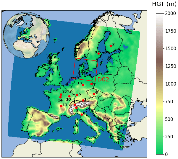
Figure 1 Modelling domains. The parent domain covers most of Europe, whereas the nested domain (D02) focuses on Denmark. The red markers, numbered from 1 to 14, indicate the location of the ICOS stations considered for model evaluation. ICOS station features are presented in detail in Table 3.

Table 1 WRF-GHG grid configuration.

2.2 Input emissions

2.2.1 Anthropogenic fluxes

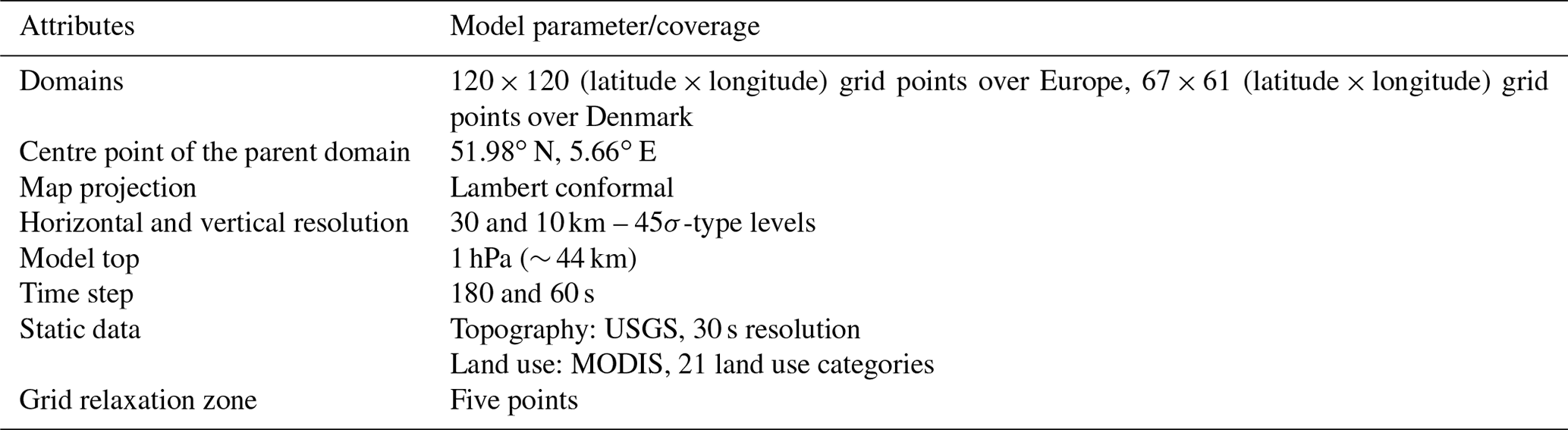
Anthropogenic fluxes of CH₄ (not including biomass burning sources) are externally prepared based on the Emissions Database for Global Atmospheric Research (EDGAR) version 6 Greenhouse Gas Emissions (Ferrario et al., 2021). EDGAR has been widely used in support of policy design for greenhouse gas emissions verification, using international statistics and a consistent Intergovernmental Panel on Climate Change (IPCC) methodology. Statistical information compiled by the IPCC Guidelines for National Greenhouse Gas Inventories (IPCC, 2006) is adopted by EDGAR for most sources and countries, complemented with information from scientific literature and other references for specific processes and/or countries. A detailed description of data providers and technical procedures for the greenhouse gas emissions of EDGAR can be found in Janssens-Maenhout et al. (2019). EDGARv6.0 includes a set of key novelties such as country/region- and sector-specific yearly profiles for all sources and country-specific weekly and daily profiles to represent hourly emissions. EDGARv6.0 CH₄ fluxes in this work include activity data from 24 different sectors that can be grouped into the following broad sectors: energy, industry, aviation, ground transport, shipping, agriculture, and waste. Biomass burning fluxes from human activities were prepared separately using a satellite-based emissions preprocessor (Wiedinmyer et al., 2023). EDGARv6.0 CH₄ fluxes are provided as monthly grid maps spatially distributed on a common grid at 0.1^∘ × 0.1^∘ resolution and can be freely downloaded at http://jeodpp.jrc.ec.europa.eu/ftp/jrc-opendata/EDGAR/datasets/v60_GHG/ (last access: 13 July 2022). Figure 2 shows the spatial distributions of CH₄ emission rates for different sectors for May 2018 in the 30 km modelling domain.

Figure 2 Spatial distribution of EDGARv6.0 CH₄ emission rates for the concerned key sectors for May 2018 in the 30 km modelling domain. Each grid point in panel (d) represents the sum of emission rates from all different sectors (except biomass burning) based on country-specific temporal profiles.

2.2.2 Biogenic fluxes

Anaerobic microbial production of CH₄ in wetlands represents the dominant source of CH₄ emissions from nature, followed by CH₄ emissions from termites. Uptake of atmospheric CH₄ by soil is the only terrestrial sink. CH₄ fluxes from natural source and sink processes are all calculated online in the model simulations. CH₄ fluxes from wetlands are based on the wetland model developed by Kaplan (2002). This model is based on a diagnostic approach that determines CH₄ emissions from wetlands as a percentage of the heterotrophic respiration following the approach of Christensen et al. (1996). The heterotrophic respiration is previously calculated based on a carbon decomposition rate and WRF-GHG variable soil moisture and soil temperature following the approach of Sitch et al. (2003). CH₄ fluxes from termites are calculated, based on the global database for termite emissions described in Sanderson (1996), as the product of the biomass of a population of termites and the flux of CH₄ emitted from that termite population. A mapping of the vegetation types used by Sanderson (1996) to the WRF-GHG vegetation type is previously performed for the quantification of the termite's biomass per grid cell. Based on WRF-GHG driving variables such as soil moisture, soil temperature, CH₄ concentration, and precipitation, soil uptake fluxes are calculated following the approach devised by Ridgwell et al. (1999). For wetland grid cells (i.e. grid cells dominated by wetlands), the calculation of soil uptake is suppressed as this process does not take place over flooded areas. It was verified that no significant natural wetlands were found over the modelling domain, with termites and soil uptake being the primary sources and sinks of CH₄ emissions in the region. Figure S1 in the Supplement shows the temporal mean spatial distribution of CH₄ emission rate for natural sources and sinks, averaged over the period from 1 to 31 May 2018.

2.2.3 Biomass burning fluxes

Biomass burning fluxes of CH₄ are externally prepared based on the Fire INventory from NCAR version 2.5 (FINNv2.5) (Wiedinmyer et al., 2023). FINNv2.5 uses satellite observations of active fires and land cover, together with emission factors and fuel loadings to provide daily, highly resolved (1 km) open burning emissions estimates for use in chemical transport models. Active fire products from both MODIS instruments onboard the Terra and Aqua satellites are applied, and to avoid double counting of the same fire on a single day, multiple detections of the fire in question are identified globally and then removed as described by Al-Saadi et al. (2008). While CH₄ fluxes from anthropogenic and biogenic sources are added at the first model level, a plume rise algorithm is applied to determine the injection height of biomass burning plumes. The plume rise algorithm, implemented in the WRF-Chem by Grell et al. (2011), is based on the 1-D time-dependent cloud model developed by Freitas et al. (2007). The algorithm is used for numerical integration for grid cells that contain fire spots, with the lower and upper limits of the injection height being calculated based on the fire category (biome burned) provided by the FINNv2.5, as well as heat flux fields inferred from WRF-GHG.

2.3 Experiment design

Initially, a model sensitivity analysis for evaluating physics schemes, such as planetary boundary layer and cumulus clouds and global forcings for meteorological fields and CH₄ concentration, was carried out over several 2-week periods in 2018 and 2019. Each of these 2-week periods were previously examined to have at least 75 % of days with TROPOMI XCH₄ data covering large portions of Europe. As a result, the physics schemes Yonsei University (YSU) for the planetary boundary layer and Kain–Fritsch for cumulus clouds, together with initial and boundary conditions from the European Centre for Medium-Range Weather Forecasts (ECMWF) Reanalysis v5 (ERA5) model (Hersbach et al., 2022) for meteorological processes and from the NCAR Community Atmosphere Model with Chemistry (CAM-chem) (Lamarque et al., 2012; Emmons et al., 2020) for background concentrations of CH₄, were selected and then used to perform a 1-year simulation period from 1 April 2018 to 31 March 2019. This period was defined based on the following criteria: (i) availability of TROPOMI XCH₄ data, (ii) latest available year data of EDGARv6.0 emissions for CH₄, and (iii) no occurrence of sustained and irregular scenarios in terms of emissions (e.g. large-scale fire outbreaks and emission reductions associated with COVID-19 lockdowns). Table 2 lists the physics and emissions schemes used in the simulations, with physics schemes other than planetary boundary layer and cumulus clouds being selected based on Beck et al. (2011). A schematic of the model running process is depicted in Appendix A. Off-line initial and boundary conditions derived from the simulations at 30 km are used as input to feed the simulations at 10 km. Model results and discussion for the nested domain are under development and will be described in a forthcoming paper.

2.3.1 Postprocessing

In order to compare the simulated XCH₄ concentrations with the observations, a set of model data postprocessing steps involving the satellite retrievals were carried out as follows. (i) The a priori profiles and averaging kernels for each orbit were regridded to the WRF-GHG discretization using a bilinear interpolation. (ii) The simulated concentrations were resampled to the SRON S5P-RemoTeC standard 12-level pressure grid. (iii) The smoothed concentrations corresponding to the resampled profiles were calculated according to the following linear transformation:

$$\begin{array}{}\text{(1)}& {\mathrm{CH}}_{\mathrm{4},\mathrm{smooth}}=\mathbf{K}\cdot {\mathrm{CH}}_{\mathrm{4},\mathrm{tot}}+\left(\mathbf{I}-\mathbf{K}\right)\cdot \mathbf{A},\end{array}$$

where CH_4,smooth represents the smoothed CH₄ concentration; A and K are the a priori profile and averaging kernel of the retrieval, respectively; I is the identity matrix; and CH_4,tot is the total CH₄ concentration. CH_4,tot is obtained by adding up the tracer contributions from the emission sources, and background concentrations are

$$\begin{array}{}\text{(2)}& {\mathrm{CH}}_{\mathrm{4},\mathrm{tot}}={\mathrm{CH}}_{\mathrm{4},\mathrm{ant}}+{\mathrm{CH}}_{\mathrm{4},\mathrm{bio}}+{\mathrm{CH}}_{\mathrm{4},\mathrm{bbu}}+{\mathrm{CH}}_{\mathrm{4},\mathrm{bgd}},\end{array}$$

where CH_4,ant, CH_4,bio, CH_4,bbu, and CH_4,bgd represent the CH₄ concentrations from anthropogenic sources, biogenic sources, biomass burning, and background concentrations. (iv) The XCH₄ concentration was finally calculated as the pressure-weighted concentration following Zhao et al. (2019):

$$\begin{array}{}\text{(3)}& {\mathrm{XCH}}_{\mathrm{4}}={\sum }_i\left[{\displaystyle \frac{P_{\mathrm{bottom}}-P_{\mathrm{top}}}{P_{\mathrm{sfc}}-P_{\mathrm{top}}}}\right]\times {\mathrm{CH}}_{\mathrm{4},\mathrm{smooth}},\end{array}$$

where P_bottom and P_top represent the pressures at the bottom and at the top of the ith vertical grid cell, and P_top and P_sfc represent the hydrostatic pressures at the top and at the surface of the model domain, respectively. Simulated total-column concentrations, without taking into account the a priori information and averaging kernels, were also computed to evaluate smoothing effects. In this case, Eqs. (2) and (3) are directly applied to the model outputs without any previous smoothing. Model evaluation against in situ CH₄ measurements is performed on the basis of the closest model grid points to the ICOS stations. Three groups of eight, six, and five ICOS stations, with sampling heights between 8.0–16.8, 40–50, and 100 m, respectively, were selected for comparison with simulated CH₄ concentrations interpolated to roughly 10, 50, and 100 m above ground level.

Table 2 WRF-GHG simulation design.

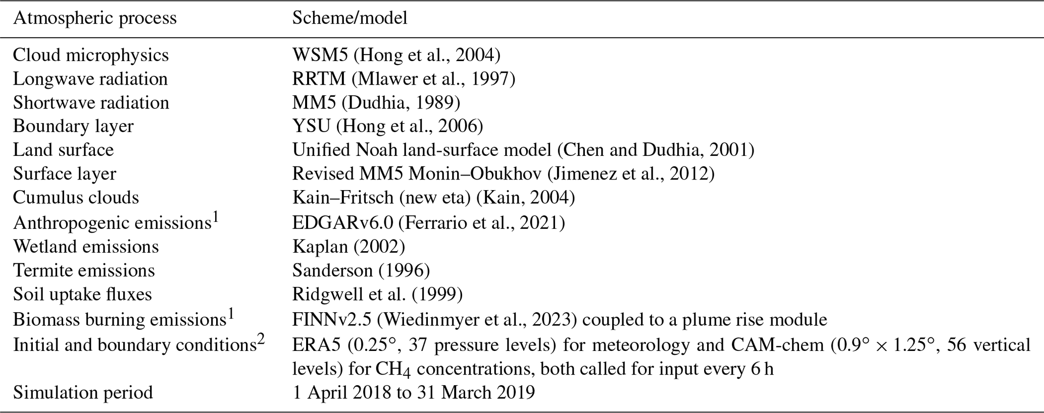
¹ The emission files for anthropogenic and biomass burning sources were processed for model input using the NCAR utilities anthro_emis and fire_emis, respectively. ² The initial and boundary conditions for CH₄ concentrations were prepared using the NCAR utility mozbc.

2.4 Observational data

2.4.1 TROPOMI

The TROPOspheric Monitoring Instrument (TROPOMI) onboard the Copernicus Sentinel-5 Precursor (S5P) satellite is a spectrometer that provides global coverage of total-column concentrations for different gases at an unprecedent resolution of 5.5 × 7 km² utilizing a push-broom configuration. The TROPOMI-based XCH₄ concentrations in this study are taken from the Netherlands Institute for Space Research (SRON) S5P-RemoTeC XCH₄ product version 17 (Lorente et al., 2022a, b), available at https://ftp.sron.nl/open-access-data-2/TROPOMI/tropomi/ch4/ (last access: 10 October 2022). In relation to the operational data products (Hu et al., 2016), the SRON S5P-RemoTeC XCH₄ product v17 provides updates regarding the regularization scheme, the selection of the spectroscopic database, the implementation of a higher-resolution digital elevation map for surface altitude, and a more sophisticated a posteriori correction for the albedo dependence. The main update with respect to the previous version, the SRON S5P-RemoTeC XCH₄ v14 (Lorente et al., 2021), includes XCH₄ retrievals over the ocean for observations made under sun-glint geometries. A quality data assessment was performed using TCCON and TANSO measurements. The TROPOMI XCH₄ data of interest to this work correspond to the recommended high-quality retrievals, with quality assurance value of 1 and for S5P orbits over Europe, i.e. with crossing times between 09:00 and 13:00 UTC.

2.4.2 ICOS

The Integrated Carbon Observation System (ICOS) is a pan-European Research Infrastructure that provides harmonized, high-precision, and long-term monitoring of atmospheric greenhouse gases. It sustains a network of stations that is spread out over different ecosystems across 12 European countries (Heiskanen et al., 2022). Greenhouse gas concentrations and meteorological parameters are usually taken at different heights of measurement towers set up in mountainous terrain or in remote environments. ICOS CH₄ concentrations in this study correspond to the fully quality-checked Level 2 data (ICOS RI, 2022), available for download at the ICOS Carbon Portal (https://data.icos-cp.eu, last access: 7 November 2022). For users interested in using ICOS data, we strongly recommend using the ICOS Carbon Portal pylib, a Python library that provides easy access to data hosted at the ICOS Carbon Portal. The ICOS stations used in this study are compiled in Table 3, and their locations are shown in Fig. 1.

Table 3 ICOS stations and atmospheric parameters considered for model evaluation.

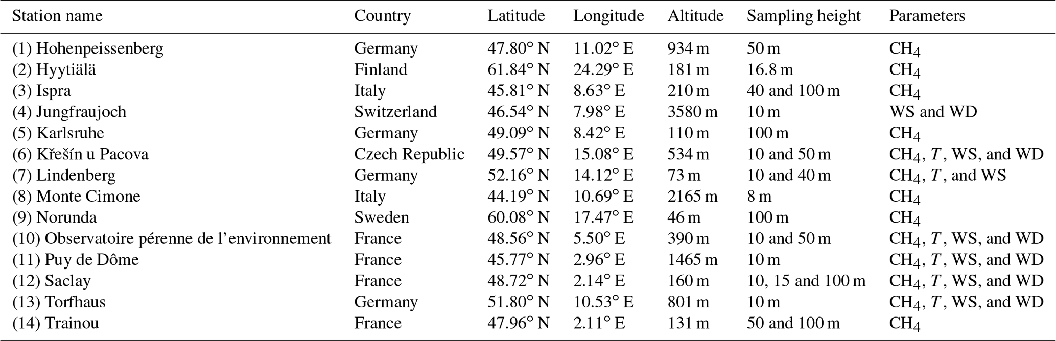
T: air temperature; WS: wind speed; WD: wind direction. CH₄ and T were interpolated to roughly 10, 50, and 100 m above ground level, while the simulated WS and WD were calculated based on the model parameters U10 and V10.

2.5 Evaluation metrics

There are a number of statistical parameters that can be used to evaluate the performance of atmospheric models, including the correlation coefficient (r), mean bias error (MBE), and root-mean-square error (RMSE). r is a measure of the strength and direction of the linear relationship between simulation and observation, MBE measures the mean difference between simulation and observation, and RMSE is the square root of the mean squared error between simulation and observation. All three are appropriate over multiple timescales and space scales and can be calculated as follows:

$$\begin{array}{}\text{(4)}& {\displaystyle }r={\displaystyle \frac{\sum \left[\left(P_j-\overline{P}\right)x\left(O_j-\overline{O}]\right)\right]}{\sqrt{\sum {\left(P_j-\overline{P}\right)}^{\mathrm{2}}x\sum {\left(O_j-\overline{O}\right)}^{\mathrm{2}}}}},\text{(5)}& {\displaystyle }\mathrm{MBE}={\displaystyle \frac{\mathrm{1}}{n}}\sum \left(P_j-O_j\right),\text{(6)}& {\displaystyle }\mathrm{RMSE}=\sqrt{{\displaystyle \frac{\mathrm{1}}{n}}\sum {\left(P_j-O_j\right)}^{\mathrm{2}}}.\end{array}$$

Here, j represents the pairing of observations (O) and predictions (P) by site and time. Overbars signify means over site and/or time. n is the number of pairs of observation–prediction values.

In conjunction with the statistics previously mentioned, graphical methods such as time series, scatter plots, and Taylor diagrams (Taylor, 2001) were also included to better understand the model behaviour over entire ranges of concentrations and gauge performance more fully. To facilitate the statistical evaluation of the model–satellite comparison, both the satellite and model data were transformed into one-dimensional arrays. Subsequently, Eqs. (4), (5), and (6) were applied to compute domain-wide statistics. Overall, as described in Sect. 3, the simulated CH₄ concentrations were in good agreement with the satellite information and near-surface measurements reported at different ICOS sites across Europe. However, several limitations and uncertainties were identified and will help to improve the model's forecast capability in future implementations.

3 Model evaluation

3.1 Near-surface CH₄ concentration

Given that the distances between the model grid points and ICOS sites can be several kilometres, it is important to highlight that the model evaluation in this section focuses more on the model's ability to reproduce the broad spatial and temporal variability in CH₄ over the modelling domain. As mentioned in Sect. 2.2.2, three sets of eight, six, and five ICOS stations, with sampling heights between 8.0–16.8, 40–50, and 100 m, respectively, were selected for comparison with simulated CH₄ concentrations interpolated to roughly 10, 50, and 100 m above ground level. Figures 3, 4, and 5 show the monthly mean spatial distributions of observed and simulated CH₄ concentrations for the first, second, and third vertical levels, respectively, with both data sets averaged over the period from 1 April 2018 to 31 March 2019. Figure S2 in the Supplement shows the monthly mean time series of CH₄ concentrations averaged over all ICOS stations and corresponding model grid points for the three levels.

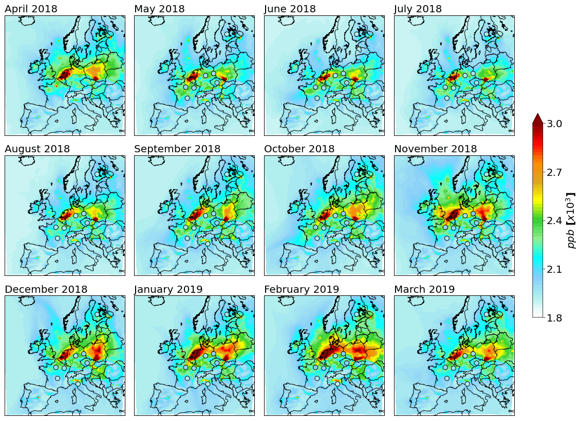
Figure 3 Monthly mean spatial distributions of simulated CH₄ concentration interpolated to roughly 10 m (shaded), together with monthly mean CH₄ concentrations from the ICOS sites with sampling heights between 8 and 16.8 m (circles), with both data sets averaged over the period from 1 April 2018 to 31 March 2019. The concentrations are in parts per billion and were computed based on quality-controlled ICOS CH₄ data for all stations simultaneously.

Overall, CH₄ concentrations for the first level were overestimated, mainly during wintertime when model–observation mismatches reached their highest values, between 200 and 300 ppb (see Fig. S2 in the Supplement). According to modelling results in this study, the simulated CH₄ concentrations depended largely on the background concentrations, followed by a small contribution from anthropogenic sources. A small month-to-month variation is observed in the CH₄ concentrations from ICOS measurements, whereas strong seasonal changes are, by contrast, observed in the CH₄ concentrations derived from model simulations – seasonal changes in the simulated concentrations are modulated by the anthropogenic sources. Using EDGARv6.0 CH₄ fluxes as the a priori emission estimates and two sets of TROPOMI-based XCH₄ observations, the global inversion approach conducted by Tsuruta et al. (2023) showed that over central Europe the anthropogenic CH₄ emissions would be slightly overestimated, mainly during spring and autumn. However, higher emission estimates are otherwise found when ground-based data are used to drive the inversions. The inversion approach for CH₄ emissions over China conducted by Hu et al. (2023) showed that the a posteriori emissions (excluding agricultural soil) decreased by 36 % compared to the EDGARv6.0 a priori emission estimates. They also found a 47.1 % reduction when it came to CH₄ emissions from waste alone. Waste emissions in EDGARv6.0 for 2018 do not have a significant daily and weekly patterns over the year, although emission peaks can be observed in February. Under real conditions, however, the production of CH₄ from waste sources depends not only on the amount of degradable organic matter but also on seasonal weather conditions (Kissas et al., 2022). Uncertainties in EDGAR emissions from other key sectors such as agriculture and energy can also contribute significantly to the overall model–observation discrepancies. For the EU27+UK (the 27 European countries and the UK), Solazzo et al. (2021) reported that while CH₄ has the best level of accuracy among the three EDGAR greenhouse gases, with only a roughly 10 % uncertainty share, the structural uncertainties in the three key sectors in terms of CH₄ (agriculture, waste, and energy) account for nearly 90 %.

Comparatively, model–observation discrepancies in CH₄ concentration at upper levels (50 and 100 m) were noticeably reduced with increasing height (see Fig. S2 in the Supplement). The bias reductions in this case are attributed to a diminishing influence of surface emissions on both magnitude and variability in CH₄ concentrations. The top-left panel in Fig. S4 in the Supplement shows the reductions in variability as a function of standard deviation, based on a site-specific comparison. The higher the sampling height (or vertical level), the smaller the model–observation discrepancies in terms of standard deviations are. Despite improvements in terms of variability, correlation coefficients remained quite similar between the three levels, ranging from 0.2 to 0.4 in most cases. Model evaluation of the global CAMS chemical modelling system against ICOS measurements, for the sites here selected and for a period 2.5 years from now (https://global-evaluation.atmosphere.copernicus.eu/ch4/ghg/insitu-icos, last access: 8 November 2022), shows structural correlation coefficients similar to those found here with WRF-GHG. However, unlike the large positive bias found in this work for the sampling height of 10 m, CAMS does underpredict the observations with model–observation discrepancies ranging from −100 to −200 ppb most of the time. In addition, no bias reduction with increasing height can be noticed in this CH₄ product. Input emissions from anthropogenic sources in CAMS simulations are built based on various existing data sets, including nationally reported emissions as well as global estimates (e.g. EDGAR; Evaluating the Climate and Air Quality Impacts of Short-Lived Pollutants, ECLIPSE; and CEDS, Community Emissions Data System). As pointed out by Solazzo et al. (2021), the fact that EDGAR has adopted the IPCC recommendations assures consistency in time and comparability across countries, but conversely, it can facilitate the propagation of uncertainties when similar emission sources are incorporated.

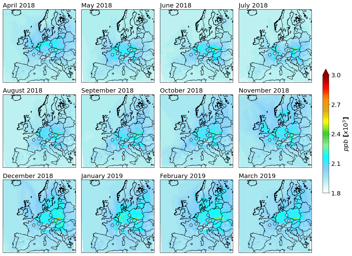
Figure 4 Monthly mean spatial distributions of simulated CH₄ concentration interpolated to roughly 50 m (shaded), together with monthly mean CH₄ concentrations from the ICOS sites with sampling heights between 40 and 50 m (circles), with both data sets averaged over the period from 1 April 2018 to 31 March 2019. The concentrations are in parts per billion and were computed based on quality-controlled ICOS CH₄ data for all stations simultaneously.

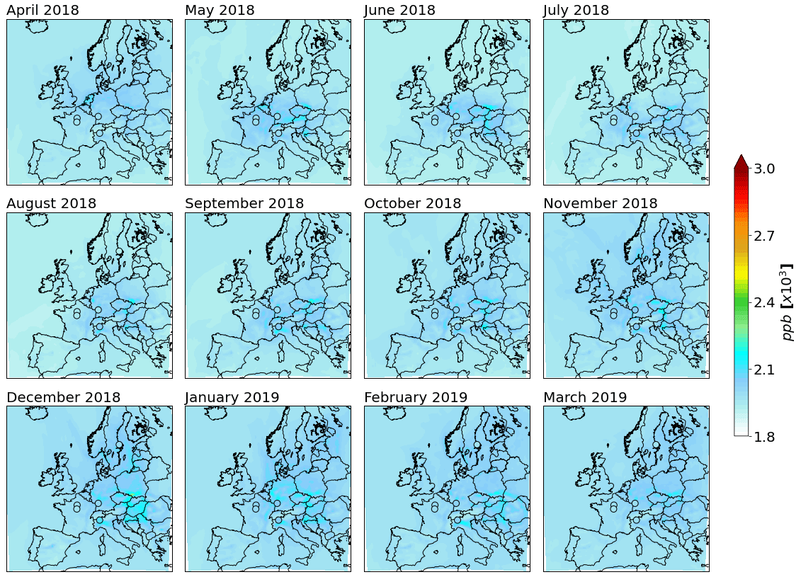
Figure 5 Monthly mean spatial distributions of simulated CH₄ concentration interpolated to roughly 100 m (shaded), together with monthly mean CH₄ concentrations from the ICOS sites with sampling heights of 100 m (circles), with both data sets averaged over the period from 1 April 2018 to 31 March 2019. The concentrations are in parts per billion and were computed based on quality-controlled ICOS CH₄ data for all stations simultaneously.

Besides errors in the CH₄ emission estimates, inaccuracies in background concentrations and meteorological conditions may have also partly contributed to model–observation discrepancies. With regard to the contribution from background concentrations, boundary conditions in the lowest model layer in CAM-chem are set to the fields specified for Climate Model Intercomparison Project – Phase 6 (CMIP6) historical conditions and future scenarios provided by Meinshausen et al. (2017). These prescribed CH₄ concentrations are then used in the model to overwrite, at each time step, the corresponding model mixing ratios (Lamarque et al., 2012). Thus, the combined effect of using uniform and projected CH₄ concentrations as lower boundary conditions in WRF-GHG simulations represents a source of uncertainty and contributes to the model–observation discrepancies. Regarding the meteorological conditions, unprecedented warmer than normal weather conditions were observed throughout the study period (Hari et al., 2020), mainly during the 2018–2019 winter season. In fact, model simulations for the period from 21 December 2018 to 14 January 2019 were not included in the model evaluation due to persistent instabilities in vertical winds over central Europe, where a sequence of heavy snowfall events has been observed (e.g. Yessimbet et al., 2022). As can be seen in Fig. S3 in the Supplement, the model overpredicted the temperature at 10 m throughout the entire winter, with overpredictions for December (averaged over 1–20 December 2018) and January (averaged over 15–31 January 2019) being much larger compared to the other winter months. Wind shifts were fairly well represented by the model, but at the same time, it did overpredict wind speed. A site-specific model evaluation in terms of correlation coefficient and standard deviation is provided in Fig. S4 in the Supplement.

3.2 XCH₄ concentration

Figure 6 shows the temporal mean spatial distributions of XCH₄ concentration from SRON RemoTeC-S5P estimates and WRF-GHG simulations, along with their relative differences, averaged over the period from 1 May to 31 August 2018. Temporal mean spatial distributions by month are shown in Figs. S5 to S16 in the Supplement. Differences between simulated XCH₄ concentrations with and without smoothing are noticeable. While relative differences between simulated concentrations without smoothing and observational data usually range from −1 % to 1 % (Fig. 6g), those between smoothed concentrations and observational data usually range from 1 % to 2 % (Fig. 6c). Model–observation discrepancies in the latter case reached their minimum values during the summer peak season (Figs. S7 to S9 in the Supplement) but otherwise reached their maximum values during winter months (Figs. S14 to S16 in the Supplement). Model performance for different seasons can be also observed in Fig. 7 which shows the monthly variability in observed and simulated XCH₄ concentrations over the study region. The lower differences between the satellite measurements and model results without smoothing were related to a CH₄ offset (against the anthropogenic emissions contribution), as the atmospheric layer above the model top (1 hPa) was not vertically integrated in Eq. (3). Simulated CH₄ concentrations and atmospheric pressures in this case did not experience any smoothing before vertical integration. Regarding the smoothed profiles, despite the fact that it was verified that the averaging kernels from satellite retrievals fluctuate slightly up and down around 1 in the troposphere (where much of atmospheric CH₄ resides), the smoothing effects in the upper levels usually lead to a XCH₄ reduction. This reduction often happens because the a priori profile (second term on the right-hand side of Eq. 1) does not influence the retrieval accuracy significantly (Hu et al., 2016). Since there is no CH₄ compensation in this case, then the bigger differences in the XCH₄ concentrations can be attributed mainly to an overestimation of anthropogenic emissions, although a systematic bias related to background signals should also be considered. At an urban scale, analysis of downwind and upwind concentrations such as the differential column methodology devised by Chen et al. (2016) can be applied to minimize the influence of background signals (e.g. Zhao et al., 2022); however, its application at a continental scale would require a high-resolution modelling configuration as well as a dense network of spectrometers. Data gaps such as those observed in central and southern Europe (Fig. 6a or e) are often produced as a consequence of applying regridding techniques to sparse data sets.

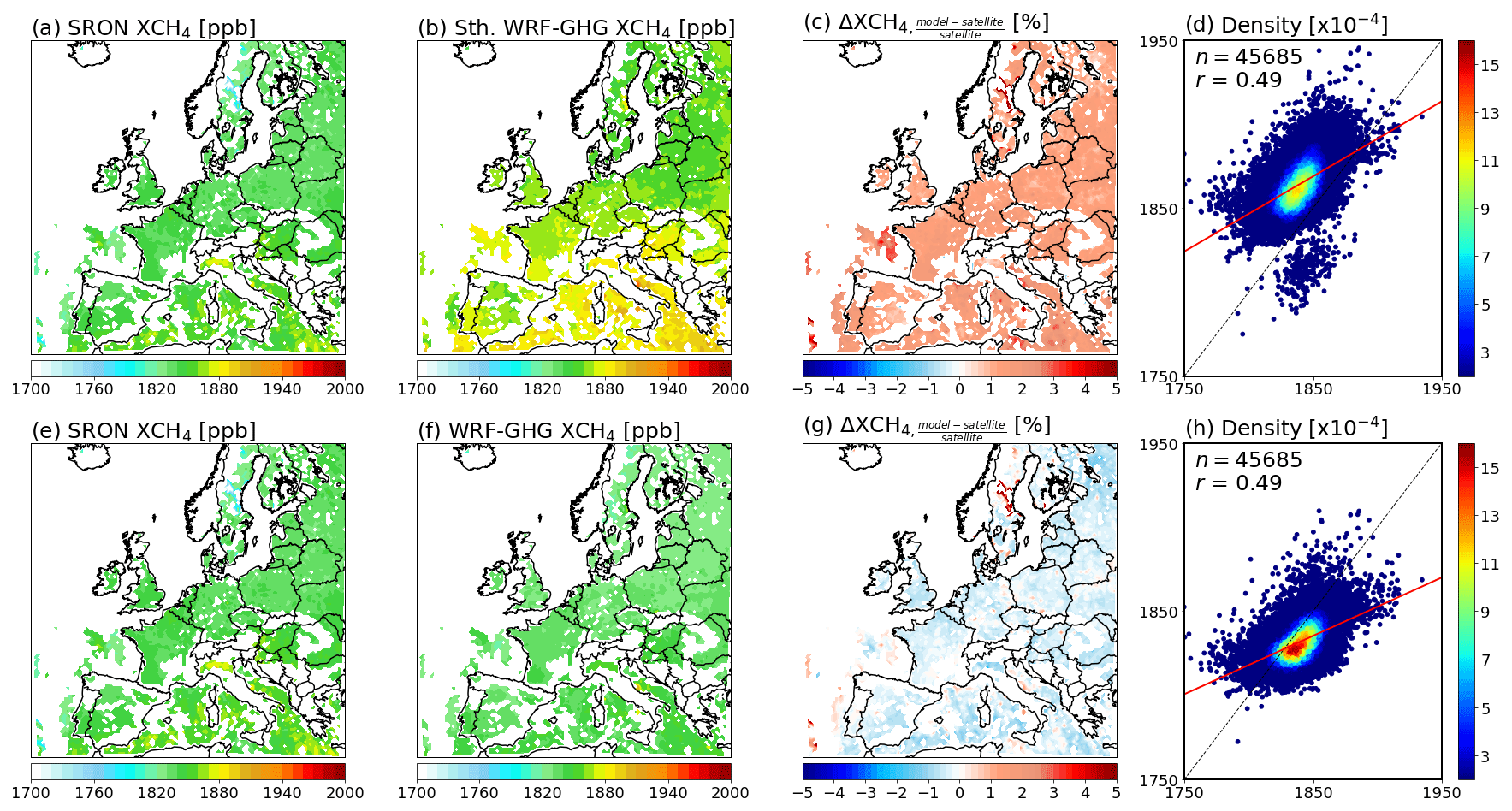
Figure 6 Temporal mean spatial distributions of XCH₄ concentration from SRON RemoTeC-S5P (a, e) and WRF-GHG estimates with and without smoothing ((b) and (f), respectively), along with their relative differences (c, g), averaged over the period from 1 May to 31 August 2018. The simulated mean XCH₄ concentrations are calculated on the basis of the closest model times to the S5P crossing times. Panels (d) and (h) show the scatter plots of observed and simulated XCH₄ concentrations, together with the number of pairs of observation–model values and the domain-wide correlation coefficient.

Zhao et al. (2019) applied the WRF-GHG model to analyse XCH₄ observations over Berlin for a period during summertime and found a bias in the simulated XCH₄ concentration of around 2.7 %. In this case, they updated the boundary conditions with information from CAMS instead of CAM-chem, used EDGARv4.1 emission estimates for anthropogenic sources, and compared the model results against total-column measurements from a network of five spectrometers. Based on the smoothed concentrations in this work, relative differences between 1 % and 2 % were often found for the summer peak season, when the anthropogenic sources had their minimum contributions to the XCH₄ concentration. For winter months, the differences were found to range from 2 % to 3 %, similar to those found by Zhao et al. (2019) for summertime. Despite the fact that a model overestimation of near-surface CH₄ concentrations on the order of 200–300 ppb is observed during wintertime, the model–observation discrepancies in XCH₄ concentration ranged roughly from 40 to 60 ppb. The higher model–observation discrepancies during winter months suggest that a more refined inverse analysis assessment will be required for this season. A recent joint inversion of CH₄ and δ¹³C-CH₄ conducted by Basu et al. (2022) for periods of relatively stability (2000–2006) and growth (2008–2014) in atmospheric CH₄ suggests a significant reduction in the a priori CH₄ emission estimates from fossil and microbial sources over northern extra-tropic regions. Bias in simulated XCH₄ concentrations over waterbodies, namely the Mediterranean Sea, the Bay of Biscay, and small portions of the Atlantic Ocean adjacent to Spain and Portugal, is of similar magnitude as that found over land. Thanks to the TROPOMI's wide swath, the SRON S5P-RemoTeC XCH₄ product v17 provides new opportunities to look into the sensitivity of CH₄ signals to surface emissions in the Mediterranean Sea (e.g. CH₄ emissions from oil and gas platforms).

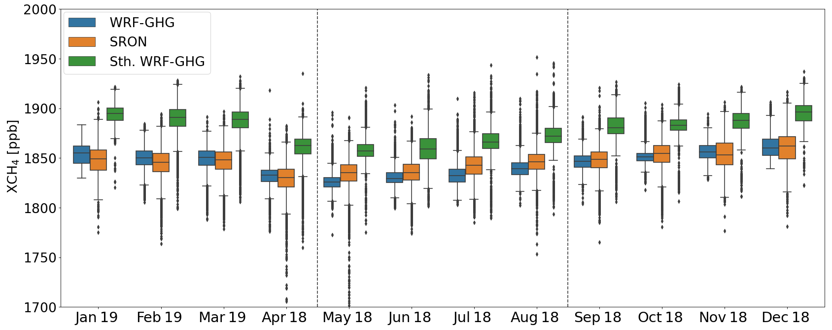
Figure 7 Monthly boxplots of observed and simulated XCH₄ concentrations with and without smoothing for the period from 1 April 2018 to 31 March 2019. The months from May to August of 2018 (between dashed lines) were selected for the model evaluation of the contribution of anthropogenic sources to the XCH₄ concentration, discussed ahead in Sect. 4.

With regard to temporal variability, a clear annual cycle of the XCH₄ interquartile range can be noticed regardless of its smooth month-to-month variation throughout the year (orange boxes in Fig. 7). Both sets of simulated XCH₄ concentrations, i.e. the simulated profiles with and without smoothing, represented this cycle fairly well although with less dispersion (length of the box). The simulated XCH₄ concentrations without smoothing show an even less dispersed interquartile range (blue boxes in Fig. 7) compared to that of the smoothed concentrations (green boxes in Fig. 7). In addition, the minimum concentrations in the simulated interquartile ranges are delayed (May) compared to observations (April), with the same happening in terms of medians. Based on the smoothed concentrations, model–observation discrepancies reached their maximum values during winter months (differences in median concentrations between 40–50 ppb), while they reached their minimum values during the summer peak season (differences in median concentrations between 20–30 ppb). As discussed in Sect. 3.2, the improved XCH₄ representation (with the simulated profiles without smoothing) responded to a CH₄ compensation, as the atmospheric layer above the model top (1 hPa) was not vertically integrated in Eq. (3). Since there is no a CH₄ compensation with the smoothed profiles, then the bigger differences in the XCH₄ concentrations can be attributed mainly to an overestimation of anthropogenic emissions. A systematic bias related to the background concentrations, however, should be also embedded in the model bias in both cases. Modelling studies using CAMS suggest that an offset between model concentrations and observations needs to be taken into account previously in the boundary conditions (Zhao et al., 2019; Gałkowsky et al., 2021). Looking at the other 50 % of data, including outliers, a similar behaviour can also be observed, with observations spread out further than simulated concentrations. A number of outliers with concentrations below 1750 ppb have been observed in April and May of 2018, although the reason why they occur in the months with the lowest CH₄ concentrations needs to be further investigated. Statistical metrics of the model–observation comparison indicate, overall, a better model performance for summer months, with correlation coefficients and root-mean-square errors ranging from 0.4–0.5 and from 27–30 ppb, respectively (see Table 4).

Table 4 Overall WRF-GHG performance against space-based XCH₄ observations. Sth.: smoothed.

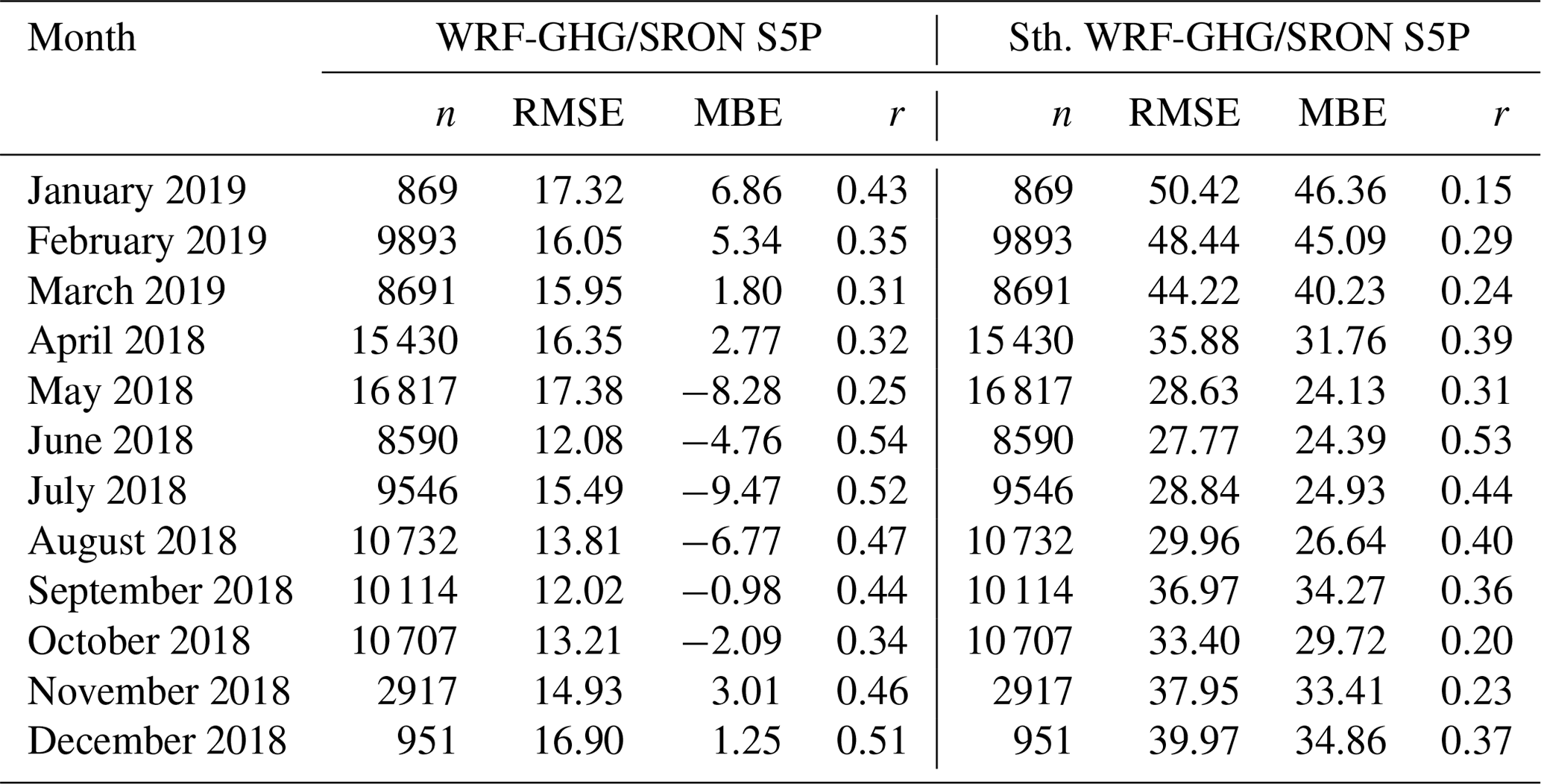
n: number of pairs of observation–model values; RMSE: root-mean-square error (in ppb); MBE: mean bias error (in ppb); r: correlation coefficient.

4 XCH₄ concentration from anthropogenic sources

The contribution of anthropogenic emissions to the XCH₄ concentration is calculated based on the months with the best model performance between May and August of 2018 (see Fig. 4). Figure 8 shows the temporal mean spatial distributions with and without smoothing of simulated XCH₄ concentrations, XCH₄ enhancement above background (EAB) concentrations, XCH₄ enhancement from human activities (EHAs) concentrations, and the contribution of anthropogenic sources to the XCH₄ concentration. Model results suggest that XCH₄ EHA concentrations as high as (or even higher than) those found over high-CH₄-emitting countries in western Europe can accumulate over countries in central and southern parts of Europe during summer months (see Fig. 8c and g). The XCH₄ EAB concentrations (Fig. 8b and f) depended almost entirely on the CH₄ contribution from human activities (Fig. 8c and g), a result that is in line with previous studies conducted over urban areas in central Europe (e.g. Zhao et al., 2019, 2022). However, the anthropogenic sources contribute only up to 2 % to the XCH₄ concentration (Fig. 8d and h), with the largest part of XCH₄ coming from background signals.

XCH₄ signals from natural sources (wetlands and termites) and biomass burning were not relevant during the study period. The inversion estimates for 2018 conducted by Tsuruta et al. (2023) showed that, compared to the anthropogenic emissions, the wetland emissions over central Europe were small, mainly during summer months when biogenic fluxes reached their minimum values. Among the factors that could have negatively influenced the accumulation of biospheric CH₄ in the atmosphere over the study region are less CH₄ formation tied to the extremely dry season in summer 2018 over central and northern Europe (Rousi et al., 2023), CH₄ compensation by soil uptake processes as the fluxes are dominated by mineral soils which are mostly net sinks of CH₄ (Tsuruta et al., 2023), and transport mechanisms. According to the Kaplan wetland map, potential natural wetlands in Europe concentrate over western regions of Russia. Yu et al. (2023) suggest that northern temperate wetland emissions in Russia show strong sensitivity to both hydrology and temperature. On the other hand, winds may disperse CH₄ concentrations out of the study region, thus reducing drastically the XCH₄ concentrations over specific regions. Both the observed and simulated wind patterns over central Europe show that, between May and August of 2018, air masses flowed mostly southeast–southwest (see Fig. S3 in the Supplement), thus deflecting most of the air coming from wetland areas. A recent study conducted by Karoff and Vara-Vela (2023) found that the XCH₄ concentrations over wetlands in Europe are lower than the average XCH₄ levels for all the land cover types analysed. They recommend, however, that before this result is verified with observations from other satellite instruments, the TROPOMI XCH₄ measurements over wetlands need to be handled with caution.

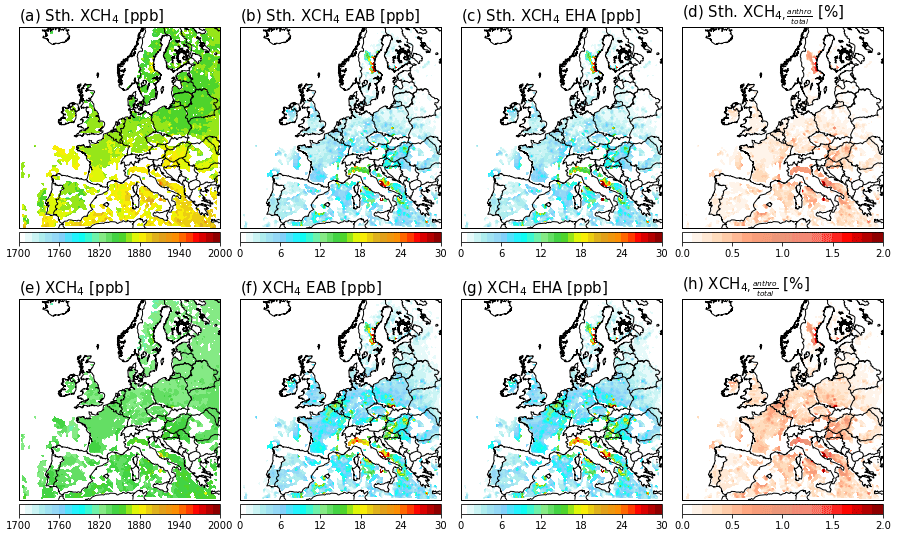
Figure 8 Temporal mean spatial distributions with and without smoothing of simulated XCH₄ concentration (a, e), XCH₄ enhancement above background (EAB) (b, f), XCH₄ enhancement from human activities (EHA) (c, g), and the contribution of anthropogenic sources to the XCH₄ concentration (d, h). Concentrations were averaged for grid points with satellite measurements during the period from 1 May to 31 August 2018, the period with the best model performance for smoothed concentrations (see Fig. 4).

5 Summary and conclusions

A new CH₄ inversion system for Europe is being implemented in order to evaluate CH₄ emission estimates from different sources, with a focus on anthropogenic activities. In this first part, the forward modelling component of the system is introduced and evaluated against CH₄ column-averaged dry air mole fractions (XCH₄) and near-surface CH₄ observations. To that end, sets of 97 h simulations for a 1-year simulation period from 1 April 2018 to 31 March 2019, were run using the WRF greenhouse gases model coupled to a multipurpose global database of CH₄ anthropogenic emissions. CH₄ fluxes from biogenic sources were calculated online in the simulations, whereas fluxes from biomass burning were externally prepared based on a satellite-based emissions preprocessor. Model results were evaluated against Netherlands Institute for Space Research (SRON) S5P-RemoTeC XCH₄ (v17) concentrations as well as against CH₄ Level 2 data from Integrated Carbon Observation System (ICOS) stations. Simulated XCH₄ concentrations without taking into account the a priori information and averaging kernels from satellite retrievals were also computed to evaluate smoothing effects.

Model–observation discrepancies on near-surface CH₄ concentration (10 m) indicate a significant overestimation on the order of 200–300 ppb during winter months. Comparatively, model–observation discrepancies on CH₄ concentration at upper levels (50 and 100 m) were noticeably reduced with increasing height. The bias reductions in this case are attributed to a diminishing influence of surface emissions on both magnitude and variability in CH₄ concentrations. In terms of XCH₄, a better representation was found with the simulated profiles without smoothing – it was related to a CH₄ offset (against the anthropogenic emissions contribution) as the atmospheric layer above the model top was not vertically integrated in Eq (3). Based on the smoothed concentrations, model–observation discrepancies reached their maximum values during winter months (differences in median concentrations between 40–50 ppb), while they reached their minimum values during the summer peak season (differences in median concentrations between 20–30 ppb). Domain-wide correlation coefficients and root-mean-square errors ranged from 0.4 to 0.5 and from 27 to 30 ppb, respectively, for summer months, and from 0.1 to 0.4 and from 33 to 50 ppb, respectively, for winter months. The higher model–observation discrepancies on XCH₄ concentration found during winter months are largely related to a significant overestimation of anthropogenic emissions; however, a systematic bias related to background signals should be also embedded in the model bias, in both scenarios with and without smoothing. The XCH₄ enhancement above background concentrations depended almost entirely on the CH₄ contribution from anthropogenic sources; however, these sources contributed with only up to 2 % to the XCH₄ concentration. XCH₄ signals from natural sources (wetlands and termites) and biomass burning were not relevant during the study period.

The results found in this study are in line with previous studies conducted over urban areas in central Europe and, thus, demonstrate a huge potential for CH₄ inverse modelling using updated TROPOMI XCH₄ data sets in large-scale applications. As discussed in Sect. 3, the model results suggest a significant overestimation of anthropogenic emissions during winter months. Therefore, for a better constraint of monthly country-scale fluxes of CH₄, an inverse analysis method taking full advantage of all satellite data available for a given month might provide much more accurate emission estimates. Ongoing work is being conducted in this direction and will be published in a second part.

Appendix A: Model running process

As a detailed description on how to run WRF-GHG can be found in Beck et al. (2011), only the initialization process, which can vary depending on specific requirements, is summarized here. Firstly, moving simulations of 97 h were performed automatically for each month so that the number of 97 h simulations in a given month constitutes a cycle in our automated bash routines. Each cycle begins, through its first moving simulation, with initial and boundary conditions previously prepared from a 7 d simulation which ends at the initialization time of the cycle at YYYY-MM-DD 00:00:00 (according to WRF-GHG date and time format). Most of this 7 d simulation is discarded as spin-up time, and only the last hour is saved to be used as initial conditions in the first moving simulation. Then, when the first moving simulation ends, the second one begins right after it with initial conditions prepared from the first moving simulation at YYYY-MM-D+1 00:00:00 and goes ahead to complete a 97 h simulation length at YYYY-MM-D+5 00:00:00. The third moving simulation will begin right after the second one ends, with initial conditions prepared from the second moving simulation at YYYY-MM-D+2 00:00:00, and will go ahead to complete a 97 h simulation length at YYYY-MM-D+6 00:00:00. This process will continue to complete the cycle, with the same procedures being applied to the other 11 remaining cycles. The boundary conditions are prepared from CAM-chem data during the preprocessing part in each moving simulation. With this methodology, all satellite data available for a given month could potentially be ingested in sets of simulations going up to 73 h backward in time. As the first day of each moving simulation is used as spin-up time, it is discarded and only the second day is used for model evaluation. The simulations were executed on LUMI (Large Unified Modern Infrastructure), which is a pan-European pre-exascale supercomputer able to provide a computing power of up to 552 petaflops.