Design and evaluation of an efficient high-precision ocean surface wave model with a multiscale grid system (MSG_Wav1.0)

Ocean surface waves induced by wind forcing and topographic effects are a crucial physical process at the air–sea interface, which significantly affect typhoon development, ocean mixing, etc. Higher-resolution wave modeling can simulate more accurate wave states but requires a huge number of computational resources, making it difficult for Earth system models to include ocean waves as a fast-response physical process. Given that high-resolution Earth system models are in demand, efficient high-precision wave simulation is necessary and urgent. Based on the wave dispersion relation, we design a new wave modeling framework using a multiscale grid system. It has the fewest number of fine grids and reasonable grid spacing in deep-water areas. We compare the performance of wave simulation using different spatial propagation schemes, reveal the different reasons for wave simulation differences in the westerly zone and the active tropical cyclone region, and quantify the matching of spatial resolutions between wave models and wind forcing. A series of numerical experiments show that this new modeling framework can more precisely simulate wave states in shallow-water areas without losing accuracy in the deep ocean while costing a fraction of the price of traditional simulations with uniform fine-gridding space. With affordable computational expenses, the new ocean surface wave modeling can be implemented into high-resolution Earth system models, which may significantly improve the simulation of the atmospheric planetary boundary layer and upper-ocean mixing.

1 Introduction

Ocean surface waves induced by wind forcing and topographic effects significantly affect the flux exchange at the air–sea interface (e.g., Garg et al., 2018; Qiao et al., 2010; Sullivan and McWilliams, 2010). Ocean surface waves can modify the underestimated intensity of tropical cyclones in coupled models by sea surface roughness and ocean spray (e.g., Bao et al., 2000; Zhang et al., 2021). They can also mitigate the overestimated sea surface temperature in summer in ocean circulation models by enhancing ocean mixing with the help of wave breaking, wave–turbulence interaction, and Langmuir circulation (e.g., Hughes et al., 2021; Zhang et al., 2012). Moreover, ocean surface waves contribute to the transport of sea surface floating litter (Higgins et al., 2020) and underwater spilled oil (Cao et al., 2021) because there are Stokes drifts as ocean surface waves propagate forward. Furthermore, driven by strong winds, disastrous waves with extreme wave heights (Wu et al., 2021) can cause huge economic losses and serious casualties with respect to coastal residents (Tao et al., 2018). Therefore, obtaining an accurate distribution of wave states in time and space is extremely important for studying atmospheric and oceanic phenomena and for guiding human production and life.

Because of their small scales with wavelengths ranging from centimeters to hundreds of meters, ocean surface waves are difficult to be resolved explicitly in large-scale numerical models (Brus et al., 2021). Widely used phase-averaged wave models only describe the statistical characteristics of wave states in every fluid unit, which is dominated by source–sink terms (e.g., WAMDI group, 1988; Yang et al., 2005). Up to now, several studies have been conducted to enhance wave simulation accuracy, such as choosing the appropriate parameterization schemes for different external forcings (e.g., Kaiser et al., 2022; Stopa et al., 2016), optimizing the parameterizations of source–sink terms (e.g., Liu et al., 2019; Zieger et al., 2015), and implementing more physical processes (e.g., Mentaschi et al., 2015; Rogers and Holland, 2009).

A higher-resolution model consisting of finer grid units can better describe complex topographic features and meandering shorelines (e.g., Chawla and Tolman, 2008; Tolman, 2003). Wave models with higher resolution can express the blocking effect of small islands better and take into account more local responses to high-precision environmental forcings, especially wind forcing. Thus, enhancing wave model resolution is also a very feasible way of obtaining high-precision wave states. However, high-resolution simulation in the whole domain can be very expensive and is limited by the available computational resources. These limitations are unconducive for operational wave forecasting that needs to predict high-precision wave states very quickly and also prevent ocean surface waves from being incorporated into high-resolution Earth system models as a fast-response physical process at the air–sea interface (e.g., Dunne et al., 2020; Jungclaus et al., 2022). Usually, in weather-scale numerical simulations, a nesting way is used to obtain local high-precision wave states and then study their effects on the air–sea interface in coupled system models. In climate-scale coupled simulations, either the wave process is not considered (Lin et al., 2020; Ziehn et al., 2020) or wave states are simulated using a coarse-resolution wave model (Bao et al., 2020; Danabasoglu et al., 2020), based on the assumption that ocean surface waves have a negligible or very small effect on the atmosphere and ocean.

Nowadays, the role of ocean surface waves in Earth system models is becoming increasingly important during this seamless climate and weather study period. The advancement of high-performance computing (hereafter HPC) also provides us with an opportunity to obtain high-precision wave states. Considering that high-precision operational wave forecasting and high-resolution Earth system models are in demand, we urgently need high-precision ocean surface wave modeling with high efficiency. After analyzing the theory that wave modeling describes the average characteristics of wave states using the wave action density spectrum as a statistical variable, regulated by the wave dispersion relation, a new wave modeling framework is designed in this paper based on a multiscale grid system with a variable grid resolution in geographical space. This paper compares the performance of this system using four numerical schemes in geographical space, reveals the different reasons for wave simulation differences in two strong-wind areas, and quantifies the matching of grid resolution between the wave model and wind signal. The optimized multiscale grid system is much finer in coastal areas but with a reasonable coarse grid spacing in open oceans. Using this grid can eliminate the disadvantages of using traditional multi-layer nesting grids. For example, it can eliminate the excessive usage of computational resources due to double calculations in overlapping areas. It can also eliminate errors caused by the downscaling process at the boundary, which will be propagated to the inner region driven by external forcings. It can still reduce uncertainty and complexity when wave models are incorporated into a multi-layer nesting Earth system model (such as the Weather Research and Forecasting (WRF) atmosphere model using a nesting and moving grid system to study typhoons).

This paper is organized as follows. In Sect. 2 the importance and constraint of high-resolution wave simulation is displayed, and the feasibility of efficient and high-precision wave modeling based on theoretical analysis of the wave dispersion relation and a series of numerical simulation experiments is analyzed. A new wave modeling framework with the unstructured triangular multiscale grid system after the comparison of different multiscale grid systems is discussed in Sect. 3. The performance of this new modeling in deep- and shallow-water areas is systematically tested and thoroughly evaluated in Sect. 4 using a series of numerical experiments. Finally, a summary and discussions are given in Sect. 5.

Table 1 Design of wave simulation experiments with different grid systems and model resolutions in Asia–Pacific areas.

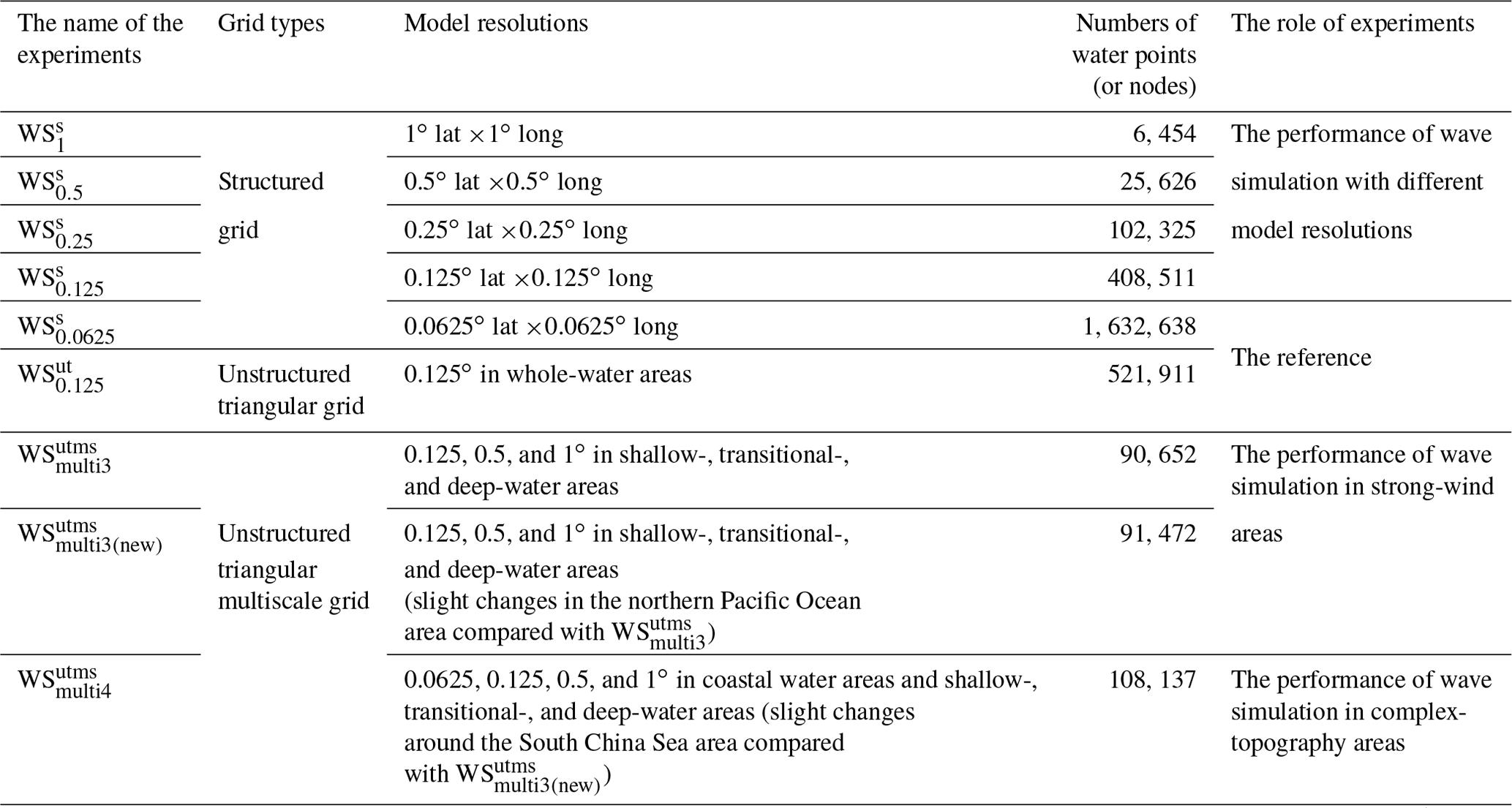
Note: to reduce the uncertainty, the maximum global time step, maximum Courant–Friedrichs–Lewy (CFL) time step for geographic and spectral spaces, and minimum source–sink term time step in all experiments are the same, which are 900 s, 90 s, 300 s, and 10 s, respectively.

2 Raising the scientific idea

2.1 The importance and constraint of high-resolution wave modeling

In this section, we first analyze the characteristics of wave simulation using traditional structured grids (or regular latitude–longitude grids) with different model resolutions by a set of experiments shown in Table 1. The design of these experiments is briefly introduced below. All physical processes in the WAVEWATCH III version 5.16 (hereafter WW3; Tolman, 1991) wave model are activated, of which parameterization settings can be referred to in Li and Zhang (2020). The needed wind forcing is from the ERA5 reanalysis dataset of the European Centre for Medium-Range Weather Forecasts (hereafter ECMWF), with a spatial and temporal resolution of 0.25^∘ and 6 h, respectively. The shoreline data can be obtained from the Global Self-consistent, Hierarchical, High-resolution Shoreline (hereafter GSHHS) dataset and the National Oceanic and Atmospheric Administration (hereafter NOAA). The topography data are from the NOAA ETOPO1 dataset with a spatial resolution of 1^′. For simplicity, we choose the Asia–Pacific area (16^∘ S–62.5^∘ N, 39–178.5^∘ E) to explain our scientific idea. The required wave boundary information is from the global wave simulation (0–359^∘, 75^∘ S–75^∘ N) using a traditional structured grid with 1^∘ resolution driven by ERA5 wind.

Driven by the same ERA5 wind, Fig. 1 shows the spatial distributions of significant wave heights (hereafter SWHs) around Taiwan (21–26^∘ N, 119–123^∘ E) in January 2018. The spatial distributions are from wave simulations (WSs) using a traditional structured grid system (“s” in the superscript) with 1, 0.5, 0.25, and 0.125^∘ model resolutions (denoted as the subscript), called WS${}_{\mathrm{1}}^{\mathrm{s}}$, WS${}_{\mathrm{0.5}}^{\mathrm{s}}$, WS${}_{\mathrm{0.25}}^{\mathrm{s}}$, and WS${}_{\mathrm{0.125}}^{\mathrm{s}}$ in Table 1. The ability to identify land and the ocean in wave models is a prerequisite for obtaining accurate wave states. However, there is an obvious mismatch between the real (surrounded by black lines, from the GSHHS dataset) and identified (white fill) locations of Taiwan and the Chinese mainland, particularly in WS${}_{\mathrm{1}}^{\mathrm{s}}$ and WS${}_{\mathrm{0.5}}^{\mathrm{s}}$ (Fig. 1a and b). Moreover, the lack of representation of some islands is a major local error source (Tolman, 2003). When model resolutions are coarse (Fig. 1a and b), the blocking effects of the Penghu islands (for example) are not expressed well. Unsurprisingly, as model resolutions increase in WS${}_{\mathrm{0.25}}^{\mathrm{s}}$ and WS${}_{\mathrm{0.125}}^{\mathrm{s}}$ (Fig. 1c and d), the above poor shoreline fitting and island representativeness are improved. Nevertheless, even if the model resolution is increased to 0.125^∘ in Fig. 1d, there is still a gap between the real and identified shorelines and topography. For instance, Green Island is too small to be resolved in wave models, which will be approximated with obstruction grids (Chawla and Tolman, 2008) (used in this paper) or parameterized with a source term (Mentaschi et al., 2015) instead.

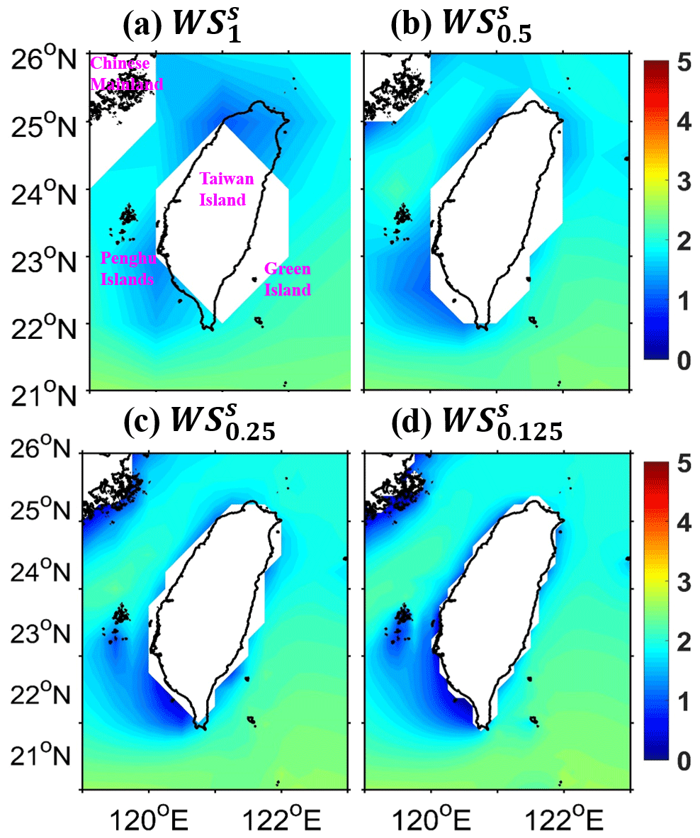
Figure 1 Spatial distributions of significant wave heights (SWHs) from wave simulation (WS) using a traditional structured grid system (“s” in the superscript) with (a) 1^∘, (b) 0.5^∘, (c) 0.25^∘, and (d) 0.125^∘ model resolutions (denoted as the subscript) around Taiwan in January 2018, called WS${}_{\mathrm{1}}^{\mathrm{s}}$, WS${}_{\mathrm{0.5}}^{\mathrm{s}}$, WS${}_{\mathrm{0.25}}^{\mathrm{s}}$, and WS${}_{\mathrm{0.125}}^{\mathrm{s}}$ (see Table 1), respectively (unit: m). The color shades and white colors indicate the ocean and land identified in the WW3 wave model with different resolutions. The areas surrounded by black lines (from the NOAA GSHHS dataset) generally represent the real land.

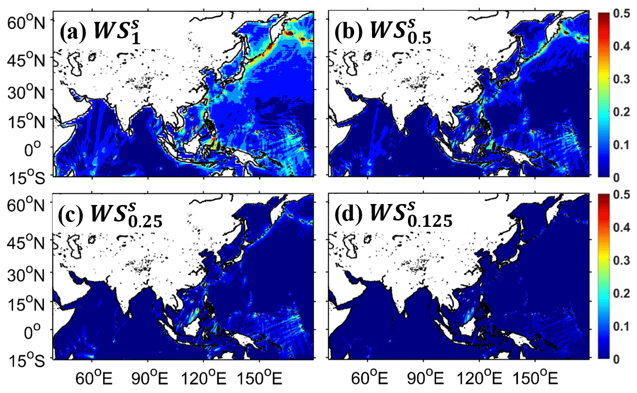
Figure 2 Spatial distributions of SWH root mean square differences (RMSDs) from (a) WS${}_{\mathrm{1}}^{\mathrm{s}}$, (b) WS${}_{\mathrm{0.5}}^{\mathrm{s}}$, (c) WS${}_{\mathrm{0.25}}^{\mathrm{s}}$, and (d) WS${}_{\mathrm{0.125}}^{\mathrm{s}}$ around the Asia–Pacific area in January 2018 (unit: m). WS${}_{\mathrm{0.0625}}^{\mathrm{s}}$ in Table 1 is considered to be a reference to calculate four SWH RMSDs by linear interpolation.

It is generally believed that the finer the model resolution, the more accurate the wave states that can be obtained. Since we do not have real wave states in the whole domain, simulation results obtained from the experiment using the structured grid with 0.0625^∘ resolutions (named WS${}_{\mathrm{0.0625}}^{\mathrm{s}}$ in Table 1) are considered to be a reference to verify the influence of different model resolutions on wave simulation accuracy. The linear interpolation method is used to calculate the SWH root mean square differences (hereafter RMSDs). Figure 2 shows the spatial distributions of SWH RMSDs around the Asia–Pacific area in January 2018. The simulated RMSDs become smaller as the model resolution gets finer. When the model resolution is 1, 0.5, 0.25, and 0.125^∘ (Fig. 2a–d), the corresponding RMSD is 0.11, 0.07, 0.04, and 0.02 m, respectively.

Figure 3 shows the time consumption of the above simulation experiments using a structured grid system under the same computational condition. When the model resolution is coarse (WS${}_{\mathrm{1}}^{\mathrm{s}}$, WS${}_{\mathrm{0.5}}^{\mathrm{s}}$, WS${}_{\mathrm{0.25}}^{\mathrm{s}}$, and WS${}_{\mathrm{0.125}}^{\mathrm{s}}$), it takes very little computational time, and we can afford it easily. However, when the model resolution is improved from 0.125 to 0.0625^∘, the consumed time increases dramatically from 1.92 to 33.79 h. The more likely reason for this phenomenon, in addition to usual reasons (an increased model resolution and a large amount of model data output), is the parallelism called card deck used in WW3. In this mechanism, one computing core calculates the wave state of one water point (not all water points in a small domain), and the wave states of two adjacent water points are calculated by different cores. See Abdolali et al. (2020) for a more in-depth understanding. The common approach to shortening computational time is to add parallel computing cores if computational resources are abundant. It is feasible when the cores used are smaller than a certain threshold. As the number of cores increases, the saved computational time can be offset by the increased time from the excessive information exchange between the cores (Feng et al., 2016). This offset situation is more obvious when you use a parallel scheme like the card deck. In addition, when computational resources are limited, it is impossible to achieve high-resolution wave simulation. In the future, if higher-resolution, longer-duration, and larger-area wave states are needed, it will require a large number of computational resources and a huge amount of time, even as expensive as atmosphere–ocean coupled models (Brus et al., 2021). This is the situation we want to prevent, and it needs to be addressed urgently.

In summary, higher-resolution wave models show better performance with respect to shoreline fitting and topography description (Fig. 1) and can simulate wave states (Fig. 2) more precisely. However, high-resolution wave simulation with a uniform fine-gridding space requires a huge number of computational resources (Fig. 3), which is a big challenge to high-precision operational forecasting systems and high-resolution Earth system models. Therefore, efficient and high-precision wave modeling is very necessary and urgent.

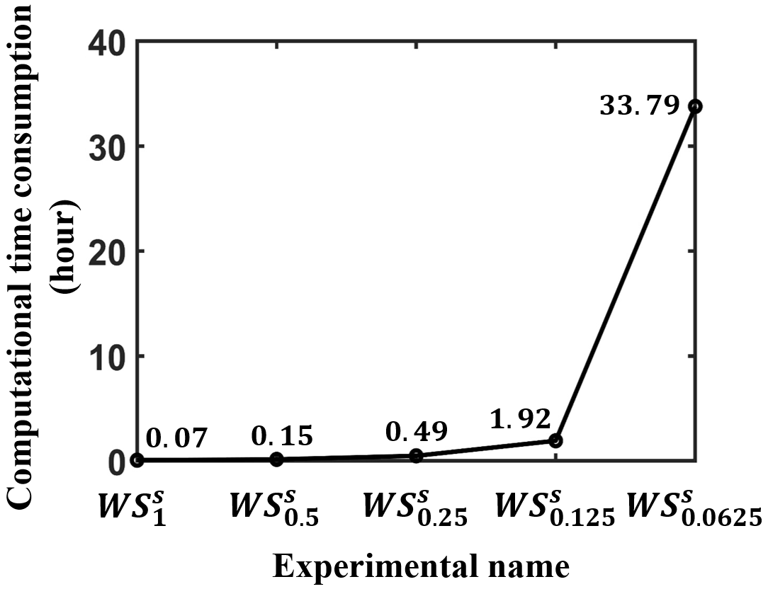
Figure 3 The computational time consumption from WS${}_{\mathrm{1}}^{\mathrm{s}}$, WS${}_{\mathrm{0.5}}^{\mathrm{s}}$, WS${}_{\mathrm{0.25}}^{\mathrm{s}}$, WS${}_{\mathrm{0.125}}^{\mathrm{s}}$, and WS${}_{\mathrm{0.0625}}^{\mathrm{s}}$ using the same computational resources (128 computing cores) to simulate 1-month (January 2018) wave states around the Asia–Pacific area (unit: h). The specific time consumption is shown at the corresponding position.

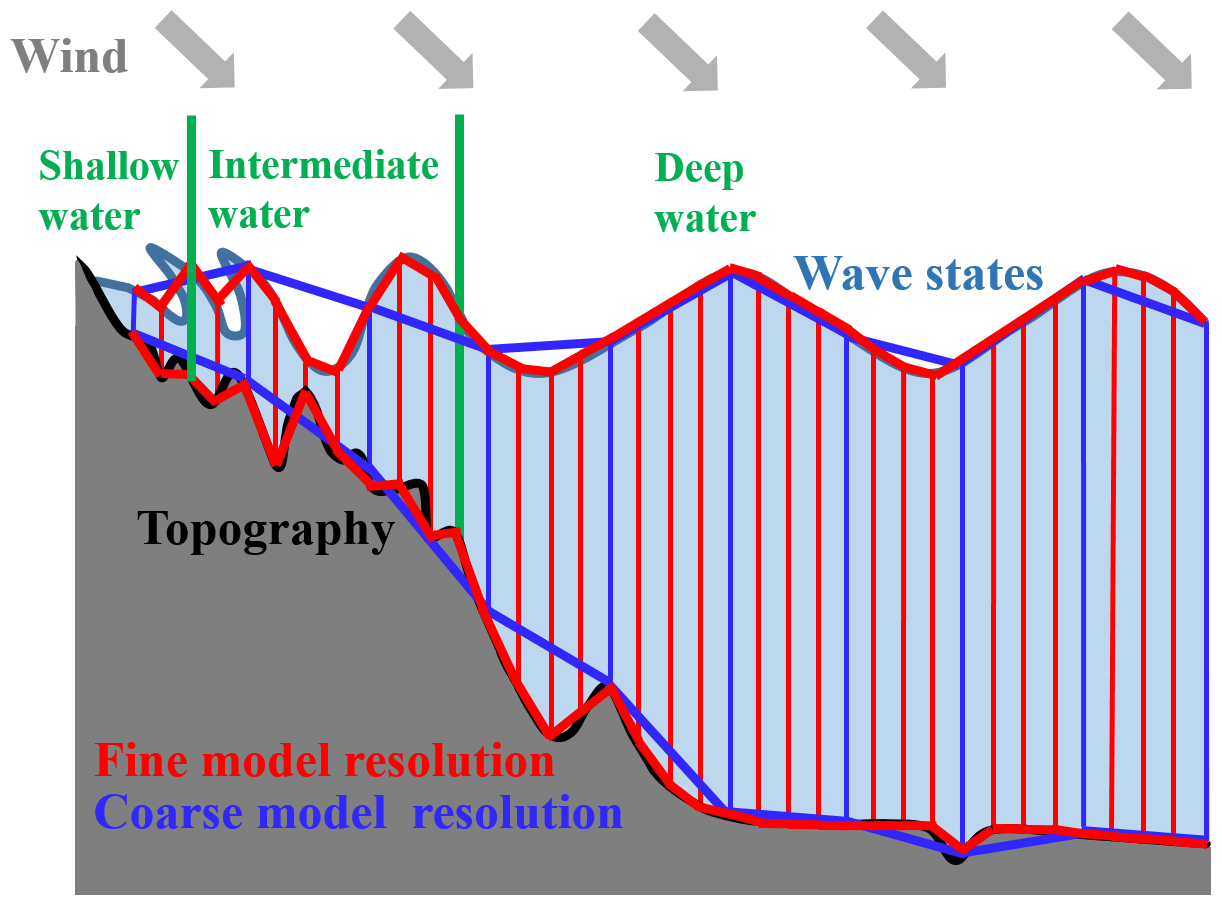
Figure 4 A schematic diagram of wave models describing complex topographic features (grey fill) and simulating wave states (navy blue lines) using fine (red lines) and coarse (blue lines) model resolutions in shallow-, intermediate-, and deep-water areas (using vertical green bars as dividing lines). The black and navy blue lines represent the actual land–ocean boundary and wave states, which are described with the thick red and blue lines in the wave models. Note that this figure does not represent the actual wave modeling process and the spatial scale of ocean surface waves.

2.2 Analysis and understanding of the wave dispersion relation

As we know, wave modeling is regulated by the wave dispersion relation; here we reintroduce it. The dispersion relation, which is the relationship between relative frequency (σ), wave number (k), and water depth (d), represents the nature and characteristics of ocean surface waves. It is expressed by σ²=gktanh (kd), where g and tanh are the gravitational acceleration and hyperbolic tangent function, respectively. In classic ocean surface wave theory, the magnitude relationship of $\frac{d}{l}>\frac{\mathrm{1}}{\mathrm{2}}$, $\frac{\mathrm{1}}{\mathrm{20}}<\frac{d}{l}\le \frac{\mathrm{1}}{\mathrm{2}}$, and $\frac{d}{l}\le \frac{\mathrm{1}}{\mathrm{20}}$ is used to determine deep-, intermediate-, and shallow-water areas, where l represents the wavelength. After a simple mathematical limit operation, the wave dispersion relation σ²=gktanh (kd) is simplified to σ²=gdk² and σ²=gk in shallow- $\left(\frac{d}{l}\le \frac{\mathrm{1}}{\mathrm{20}}\right)$ and deep-water $\left(\frac{d}{l}>\frac{\mathrm{1}}{\mathrm{2}}\right)$ areas, respectively.

To more vividly show the meaning of the wave dispersion relation, a schematic diagram of wave propagation characteristics described in different water areas and simulated with different spatial resolutions is shown in Fig. 4. In deep-water areas, ocean surface waves have large wavelengths and long wave periods. Because they are insensitive to topographic features (represented by water depth d in the above dispersion relation), wave models with coarse or fine resolution, consisting of coarse or fine grid units, have good performance in simulating wave states almost without losing accurate responses to wind signals. When ocean surface waves travel from deep- to intermediate-water areas (their boundary is marked with a vertical green bar), the wavelength decreases, and the wave height increases. The effects of topographic features (thick black line) on the wave states are activated. These features (such as sea peaks and valleys) are well represented (excessively smoothed) using fine-resolution (coarse-resolution) models, shown with thick red lines (thick blue lines), which directly affects wave simulation accuracy. Moreover, when ocean surface waves reach coastal areas with very shallow water, more complex physical processes should be considered, such as depth-induced wave breaking, wave scattering, and reflection, etc. However, the described topographic features are distorted even when using fine-resolution models, let alone coarse-resolution models. This situation directly leads to very poor simulation precision (as shown in Fig. 1d). Thus, wave model resolution needs to be improved constantly, especially in coastal areas. It is worth mentioning that Fig. 4 is a schematic diagram and does not represent the actual wave modeling process (using the wave action density spectrum as the integral variable) and spatial scales of ocean surface waves – it only illustrates our idea.

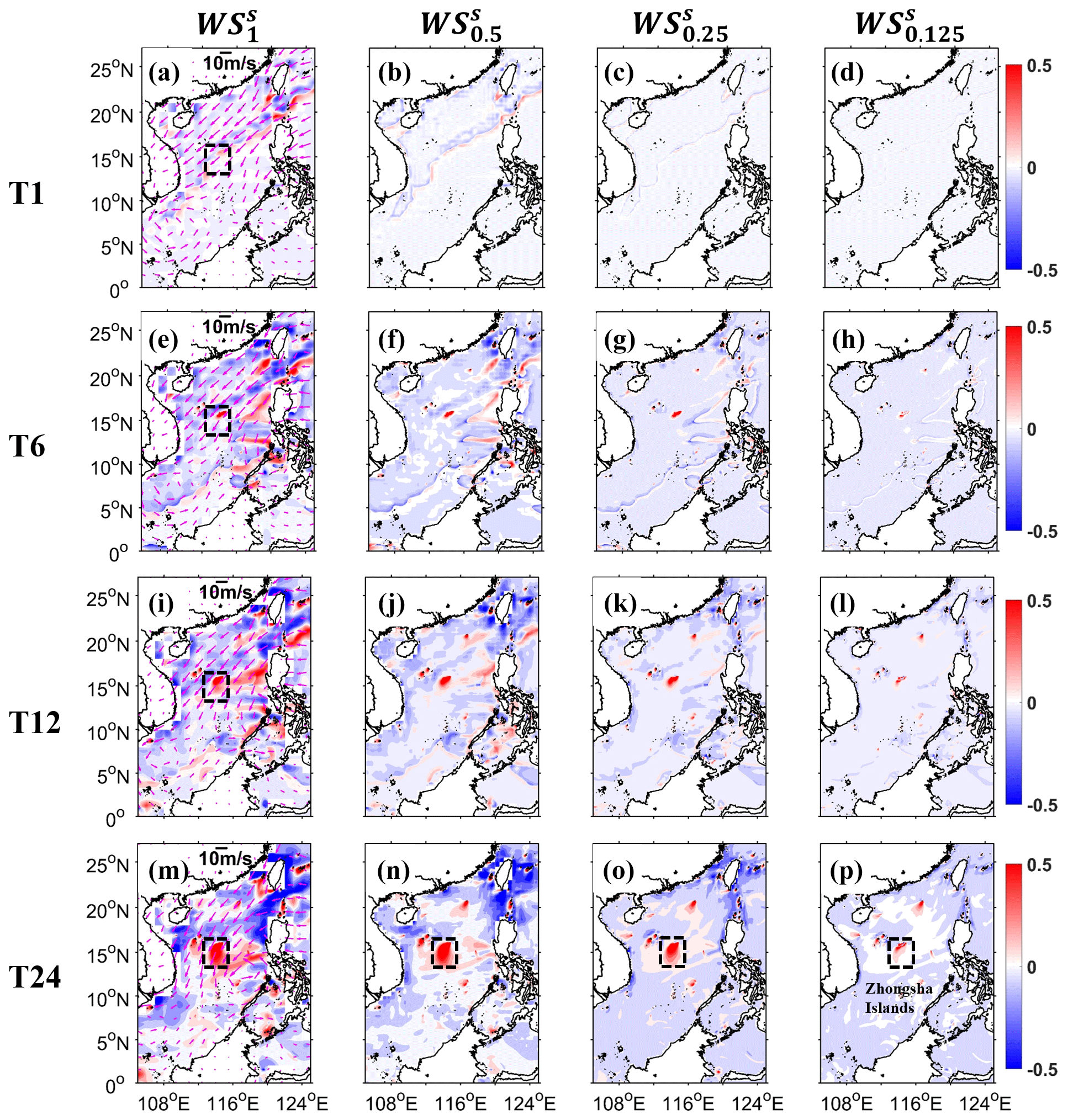
Figure 5 Spatial distributions of SWH differences from WS${}_{\mathrm{1}}^{\mathrm{s}}$ (a, e, i, m), WS${}_{\mathrm{0.5}}^{\mathrm{s}}$ (b, f, j, n), WS${}_{\mathrm{0.25}}^{\mathrm{s}}$ (c, g, k, o), and WS${}_{\mathrm{0.125}}^{\mathrm{s}}$ (d, h, l, p) around the South China Sea at 01:00, 06:00, and 12:00 UTC, 1 November 2017 (the first, second, and third rows, named T1, T6, and T12), and 00:00 UTC, 2 November 2017 (the fourth row, named T24) (note that the wave states of all experiments at 00:00 UTC, 1 November 2017, are resting) (unit: m). The magenta arrows in the first column (a, e, i, m) are wind vectors for the corresponding moment (unit: m s⁻¹). The Zhongsha Islands are framed by dashed boxes in the first column and the last row. WS${}_{\mathrm{0.0625}}^{\mathrm{s}}$ in Table 1 is considered to be a reference to calculate SWH differences by linear interpolation (interpolated results minus the reference).

Next, we use numerical simulation results to further understand the above theoretical characteristics. The wave simulation using a structured grid with 0.0625^∘ resolutions is regarded as the reference experiment and that with 1, 0.5, 0.25, and 0.125^∘ resolutions separately is regarded as a control experiment (four control experiments in total). Figure 5 shows the evolution of SWH differences (control minus reference, representing errors) around the South China Sea (0–27^∘ N, 105–125^∘ E) on the first day of model integration. The wave states are resting at the first moment of the model run (00:00 UTC, 1 November 2017). After that, ocean surface waves begin to generate and propagate, induced by wind forcing and topographic effects. Driven by strong wind (magenta arrows in the first column of Fig. 5), ocean waves in the northwestern South China Sea have rapid responses at the first integral time step (00:15 UTC, 1 November 2017). Because coarse-resolution models lack representation of complex topography (WS${}_{\mathrm{1}}^{\mathrm{s}}$ for example), SWH differences are generated at the beginning of the model run. They are propagated forward, driven by wind, which can be observed clearly at the fourth integral time step in Fig. 5a. As time passes, the simulated differences are constantly generated and propagated to the deep ocean, driven by the strong wind (Fig. 5e and i). At the 24th hour of model integration, they are almost distributed over the whole South China Sea (Fig. 5m). At the same time, driven by weak wind, SWH differences are small, and their effects on the surrounding sea areas are relatively weak in the southeastern South China Sea (the first column of Fig. 5). As we expected, with the increase in model resolution, there is a higher representation of topographic features and a more accurate response to local wind, so the simulated differences gradually decrease. They are almost imperceptible when the model resolution is 0.125^∘ (WS${}_{\mathrm{0.125}}^{\mathrm{s}}$, the fourth column). See Zhongsha Islands framed by dashed boxes in the first column and last row for a more in-depth observation.

2.3 On the feasibility of efficiently modeling ocean surface waves

Based on the above theoretical analysis and numerical simulation, we have the following understanding. (1) In shallow- and intermediate-water areas, wave states are very sensitive to topographic features, especially in coastal areas. Therefore, a finer-resolution wave model consisting of smaller fluid units is necessary to better describe the complex topographic features and meandering shorelines. This can reduce wave simulation errors in shallow-water areas and weaken their effects on the surrounding sea areas. It also takes into account more local responses driven by high-precision environmental forcings, especially wind forcing. (2) In deep-water areas, wave states are insensitive to topographic effects. Hence, a coarse-resolution model is suggested to save computational resources without sacrificing accurate responses to external forcings.

Therefore, similar to the classic wave theory, we choose the magnitude relationship between $\frac{d}{l}$ and $\frac{\mathrm{1}}{\mathrm{2}}$ to determine shallow- $\left(\frac{d}{l}\le \frac{\mathrm{1}}{\mathrm{2}}\right)$ and deep-water $\left(\frac{d}{l}>\frac{\mathrm{1}}{\mathrm{2}}\right)$ areas for simplification. Here, the shallow-water areas are a general notion, including the shallow- and intermediate-water areas defined in classic theory, where topographic effects should be taken into account in wave simulation. It is important to note that we only follow the idea of dividing different water areas from the classic theory and do not change the expression of the wave dispersion relation in all numerical simulation experiments. Previous studies have used a specific/gravity water depth as a criterion to classify different waters (e.g., Brus et al., 2021; Li, 2012; Mao et al., 2015), which has achieved good results in saving wave simulation time. The method used in this paper is a direct application of the wave dispersion relation, which can minimize the number of fine grids. This will further improve wave simulation efficiency, which is needed very much for the Earth system models considering the ocean surface wave process.

Therefore, we can design a new wave modeling framework with a multiscale grid system that is much finer in coastal areas but relatively coarse in open oceans, to achieve efficient and high-precision wave simulation. This wave modeling idea is preliminarily feasible, since the global ocean is almost completely covered by deep water, with only a small portion of shallow water, such as only 2.7 % of shallow water in the Asia–Pacific area. Next, we introduce in detail the different implementations of building this framework, the factors to consider for designing a multiscale grid system, and the performance of this framework.

3 Design of an efficient and high-precision wave modeling framework

3.1 Multiscale grid systems

Multiscale grid systems are usually made up of multiple polygons with different spatial sizes. Currently, two multiscale grid systems are available in wave models. One is made up of rectangles with different sizes (Li, 2011), named the unstructured rectangular multiscale grid in this paper. The other is made up of triangles (e.g., Roland et al., 2009; Zijlema, 2010), called the unstructured triangular multiscale grids (“utms” for short, superscripts of experiment names in Table 1). They have similar design ideas, setting fine-resolution meshes in shallow-water areas to enhance simulation accuracy and coarse-resolution meshes in deep-water areas to save computation resources. At the same time, to avoid a sharp gradient in coastal water depth, setting modest-resolution meshes in transitional-water areas ensures a stable calculation. Note that the transitional-water areas here are part of deep-water areas, which are different from the intermediate-water areas in classic wave theory. Now, using simple diagrams in Fig. 6, the generation steps of these two grids both with variable resolutions from Δx in shallow-water areas to 2Δx in transitional-water areas and then to 4Δx in deep-water areas and their performance are briefly introduced. Note that curvilinear grids as an extension of traditional structured grids (Rogers and Campbell, 2009) are not discussed here.

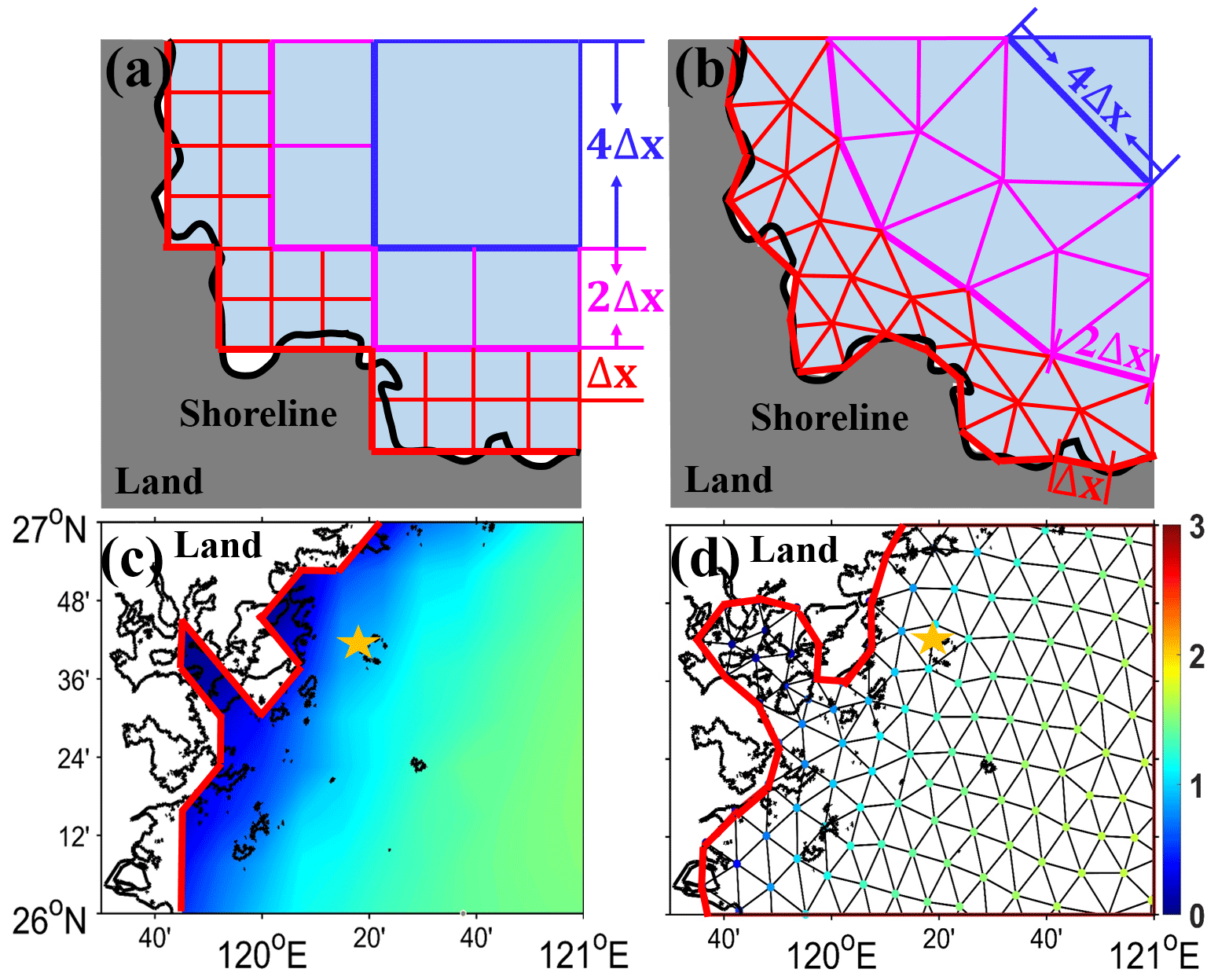
Figure 6 A diagram of unstructured (a) rectangular and (b) triangular multiscale grid systems with Δx, 2Δx, and 4Δx spatial resolutions in shallow-, transitional-, and deep-water areas marked with red, magenta, and blue lines. Spatial distributions of SWHs are from wave simulation using (c) a traditional structured grid and (d) an unstructured triangular grid, both with a fine resolution (named WS${}_{\mathrm{0.125}}^{\mathrm{s}}$ and WS${}_{\mathrm{0.125}}^{\mathrm{ut}}$ in Table 1) in July 2018 (unit: m). The Chinese oceanic station named BSG is located at 26.7^∘ N, 120.3^∘ E and is marked with yellow stars in (c) and (d). The thick black and red lines are the actual and described land–ocean boundaries in the four panels.

3.1.1 Generation of multiscale grid systems

The steps for making unstructured rectangular multiscale grid systems are described as follows (Hou et al., 2022). The study area can be divided into 2×2 rectangular groups with 4Δx resolutions. Looping for every group, if there is no land inside, the group is marked with blue lines in Fig. 6a. Otherwise, the group can further be divided into 2×2 boxes with 2Δx resolutions. Similarly, looping for every box, it is marked with magenta lines if the box is covered with water everywhere. Or, the box is divided into 2×2 cells with Δx resolution. Cells near shorelines can be identified as land or ocean by judging the land–ocean ratio in every cell. The actual and fitted shorelines are marked with thick black and red lines, respectively. Now, the unstructured rectangular multiscale grid is generated. Note that the scale of two adjacent meshes is 1:1 or 1:2.

The steps of generating an unstructured triangular multiscale grid are described in the following. In the beginning, obtaining fine shoreline data is necessary. Next, with the help of shorelines and two types of control lines marked with thick red, magenta, and blue lines in Fig. 6b, the spatial resolution in shallow-, transitional-, and deep-water areas can be set to Δx, 2Δx, and 4Δx, respectively. Once reasonable control lines are ready, a lot of triangles with different spatial sizes are generated quickly, completing the unstructured triangular multiscale grid. Note that if the grid resolution is set to 4Δx, this does not mean that the length of three elements in every triangle is exactly 4Δx but that it varies within a reasonable range around 4Δx (±20 % used in this paper).

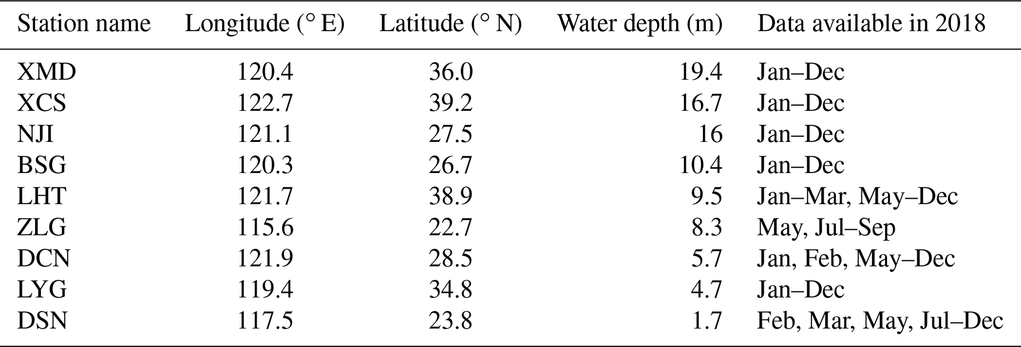
Table 2 Information pertaining to the Chinese oceanic observation stations used in this paper.

3.1.2 Comparison of two grid systems

Here we further compare the performance of wave simulation using different grid systems with the same fine resolution. The lower panels of Fig. 6 show spatial distributions of SWHs from wave simulation using the traditional structured and unstructured triangular grids, both with 0.125^∘ resolutions (named WS${}_{\mathrm{0.125}}^{\mathrm{s}}$ and WS${}_{\mathrm{0.125}}^{\mathrm{ut}}$ in Table 1; Fig. 6c and d show wave states in a small area of the Asia–Pacific region for clarity). The finest spatial resolution (0.125^∘) is used in the entire region in Fig. 6c and d, just as the finest spatial resolution (Δx) is set throughout the whole domain in the upper panels (Fig. 6a and b). Compared to those using the structured grid (red lines in Fig. 6c), wave models using the unstructured grid (red lines in Fig. 6d) have a better ability to fit the actual land–ocean shorelines (black lines in Fig. 6c and d). This is the reason why the latter has simulation results at all nine available Chinese oceanic stations that are very close to shorelines (Table 2), while the former has simulation data only at four stations, including XCS, NJI, BSG, and DCN. Since wave simulation using different grids performs similarly at these four stations, the results at station BSG are used here as an example for illustration purposes. This station is marked with yellow stars in Fig. 6c and d near a group of small islands (a distance from the mainland), which are not enough to be resolved in wave models using structured or unstructured grids with 0.125^∘ resolutions. The former uses sub-grid obstacles with different levels of transparency for approximation, while the latter directly treats them as water areas. When waves travel from the open ocean to the mainland in a southeastern direction, ocean surface waves at this observation station behind these islands are underestimated resulting from a lot of wave energy dissipation caused by excessive blocking in wave models using a structured grid. For example, the observed average SWH is 1.28 m at the valid observed time in July 2018, and the simulated SWHs are 1 and 1.23 m in WS${}_{\mathrm{0.125}}^{\mathrm{s}}$ and WS${}_{\mathrm{0.125}}^{\mathrm{ut}}$ (Fig. 6c and d), respectively. Therefore, wave models using the unstructured triangular grid have more advantages than those using the traditional structured grid in shoreline fitting and coastal simulation accuracy, while they take almost the same computational time (2.04 and 1.92 h in Fig. 13).

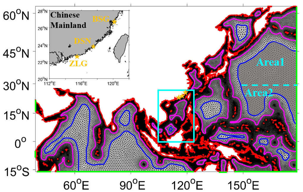
Figure 7 The spatial distribution of the new wave modeling framework using an unstructured triangular multiscale grid system. Grid resolutions vary from 0.125^∘ in shallow-water areas to 0.5^∘ in transitional-water areas and then to 1^∘ in deep-water areas, with the help of the shorelines (red) and two types of control lines (magenta and blue), named WS${}_{\mathrm{multi}\mathrm{3}}^{\mathrm{utms}}$ in Table 1. The green lines represent the spatial locations of the open boundary. The Chinese oceanic stations named BSG (the same station in Fig. 6), DSN, and ZLG are marked with yellow stars, and the top-left panel is a clearer display. In Sect. 4, this framework is further developed in two areas. The first is the northern Pacific Ocean area with a grey fill (surrounded by a blue line) $\left({\mathrm{WS}}_{\mathrm{multi}\mathrm{3}\left(\mathrm{new}\right)}^{\mathrm{utms}}\right)$. The second is around the South China Sea area framed by a solid cyan box $\left({\mathrm{WS}}_{\mathrm{multi}\mathrm{4}}^{\mathrm{utms}}\right)$. See the corresponding section for details.

3.2 Design of a new wave modeling framework

Considering the advantages of triangular grids in coastal areas (e.g., Engwirda, 2017; Roberts et al., 2019) and the follow-up sustainability of this work, we design the first version of a new wave modeling framework using an unstructured triangular multiscale grid to achieve the goal of efficient and high-precision wave simulation. The generated steps in Surface-water Modeling System (SMS) software are described as follows. Similar to previous papers, we first empirically set the spatial resolution of this multiscale grid in different water areas. In the next section, we optimize this grid after evaluating its performance through a series of experiments. Finally, we give a few tips for designing the grid resolution, particularly in deep-water areas, which is easy for readers to follow.

•  

  Step 1 – obtaining and optimizing shorelines. Theoretically, with the support of high-resolution topography and shoreline datasets, mesh resolution can be refined infinitely (e.g., Li and Saulter, 2014) in shallow-water areas to simulate higher-precision wave states. Fine shoreline data come from the NOAA GSHHS dataset with a 1 km resolution, and topography data come from the NOAA ETOPO1 dataset with a 1^′ resolution. In practice, trading off the simulation accuracy and computational resource consumption, we set the shoreline resolution to 0.125^∘ (red lines in Fig. 7) for a preliminary test. Proper shoreline adjustment is suggested if there is any unsuitability, which is very important to accurately obtain coastal wave states (Fig. 6d). When finer shoreline data are available in key areas, the shorelines should be further refined if necessary.

•  

  Step 2 – setting control lines with different spatial resolutions. As stated in Sect. 2.2, wave states are insensitive to topographic features in deep-water areas, which can be simulated using coarse-resolution models. Here, we determine the boundary locations between shallow- and deep-water areas (their definitions differ from the classic definitions and are introduced in Sect. 2.3) based on the relationship between the water depth and half of the minimum mean wavelength. These two variables are derived from wave simulation results with a resolution of 0.0625^∘ (WS${}_{\mathrm{0.0625}}^{\mathrm{s}}$ in Table 1) in 2018. Then, the control lines following this boundary can be set to 0.5^∘ (magenta lines in Fig. 7). To further shorten the computational time, we set other control lines with 1^∘ resolution (blue lines in Fig. 7) in the deeper ocean, where the global grid resolution is suggested in Tolman (2003). Note that the spatial locations of these two types of control lines are adjusted by constant testing to achieve a stable calculation and maximum benefit.

•  

  Step 3 – generating the unstructured triangular multiscale grid. Once reasonable control lines and open boundaries (green lines in Fig. 7) are determined, a lot of triangles with different spatial sizes are quickly generated in SMS. This software has a powerful function to identify poor-quality meshes (just a tiny fraction of the total meshes), such as one node connecting too many elements (eight used in this paper) or a triangle with too big (130^∘ used in this paper) or too small (30^∘ used in this paper) interior angles. It is recommended to adjust these poor-quality meshes to ensure stable computation, which takes very little time.

Now, the first version of the wave modeling framework using the unstructured triangular multiscale grid with the spatial resolutions of 0.125, 0.5, and 1^∘ in shallow-, transitional-, and deep-water areas is finished (WS${}_{\mathrm{multi}\mathrm{3}}^{\mathrm{utms}}$ in Table 1). Figure 7 shows that the spatial size of these meshes gradually and smoothly increases from coastal areas to deep oceans with the help of control lines.

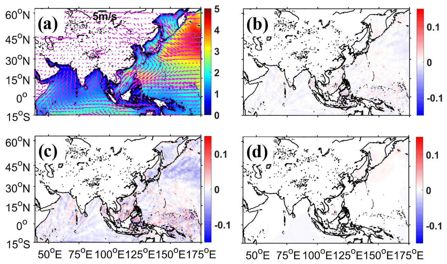
Figure 8 (a) Spatial distributions of SWH from WS${}_{\mathrm{multi}\mathrm{3}}^{\mathrm{utms}}$ using the CRD-N propagation scheme and monthly mean wind vectors (magenta arrows) in January 2018 (unit: m for SWH and m s⁻¹ for wind vectors). (b–d) Spatial distributions of SWH differences from WS${}_{\mathrm{multi}\mathrm{3}}^{\mathrm{utms}}$ using the CRD-PSI, CRD-FCT, and implicit N propagation schemes, respectively, minus that using the CRD-N scheme (Fig. 8a) (unit: m).

4 Evaluation of wave simulations

4.1 Evaluation with different propagation schemes

Wave models describe the evolution of the wave action density spectrum in the geographic space (including longitude and latitude) and spectral space (including frequency and direction), dominated by source–sink terms. Since we only change the grid size in the geographic space, here we evaluate the performance of wave simulation using the unstructured triangular multiscale grid (WS${}_{\mathrm{multi}\mathrm{3}}^{\mathrm{utms}}$ in Table 1) in this space. There are four propagation schemes available in wave model WW3, including CRD-N, CRD-FCT, CRD-PSI, and implicit N. See Roland (2009) for more detailed descriptions. After a 14-month numerical integration (from 00:00 UTC, 1 November 2017, to 23:00 UTC, 31 December 2018) using four numerical schemes separately, WS${}_{\mathrm{multi}\mathrm{3}}^{\mathrm{utms}}$ can run stably. This indicates that it is feasible that wave energy can propagate smoothly and continuously on multiple meshes with different spatial resolutions. Wave simulation results using four spatial propagation schemes and their comparison are shown in Fig. 8, and the duration of their computation time is listed in Table 3.

Figure 8a displays SWH distributions of wave simulation using the propagation scheme CRD-N (the default scheme, first-order precision in time and space) in January 2018 (the month with the largest differences when wave simulation uses four numerical schemes in 2018). There is a high correlation between the magnitude of wave height (color shaded) and wind intensity (magenta arrows); for example, in the northern Pacific Ocean (the northern Indian Ocean and equatorial Pacific region), ocean surface waves have large (small) wave heights driven by strong (weak) wind. Figure 8b–d show the SWH differences between wave simulation using CRD-PSI, CRD-FCT, and implicit N schemes, respectively, and those using the CRD-N scheme (Fig. 8a). The differences between wave simulation using nonlinear CRD-PSI and linear CRD-N schemes are relatively small (Fig. 8b), and the spent calculation time of these two experiments is roughly the same (Table 3). Roland (2009) mentioned that the CRD-PSI scheme is second order only in the cross-flow direction and is first order in the longitudinal flow direction and time. There are obvious simulation differences in Fig. 8c, and they propagate forward, driven by wind (wind vectors shown in Fig. 8a). This is because CRD-FCT has second-order precision in time and space, and, by using this scheme with respect to wave simulation, it is easier to produce differences in complex topographic areas (especially in the archipelago region of the eastern equatorial Pacific Ocean) compared with using the linear CRD-N scheme. Also, using the CRD-FCT scheme leads to the lowest calculation efficiency among the four schemes (Table 3). There are only slight differences in Fig. 8d because the CRD-N and implicit N schemes both use a linear scheme. Although there are differences in wave simulation results using four schemes, these differences are almost within a scale of ±0.1 m, which is negligible. Similar performance is given after verifying with observations at nine available Chinese oceanic stations (Table 2) (not shown). The wave parameters of the mean wave period (hereafter MWP) and mean wave direction (hereafter MWD) also have negligible simulation differences (not shown). On the whole, wave simulation with the explicit and implicit schemes has a similar simulation accuracy for Courant–Friedrichs–Lewy (CFL) <1 (WW3DG, 2019). It should be noted that when wave simulation uses multiscale grid systems, it is better to extend the computing area outward by 3^∘ (1^∘ spatial resolution at most boundary areas) to reduce the influence of open boundaries on the concerned area, especially if the wave model uses the CRD-FCT scheme that has a two-order precision.

Wave simulation results using the unstructured triangular grid with 0.125^∘ resolutions in the whole domain (WS${}_{\mathrm{0.125}}^{\mathrm{ut}}$ in Table 1) are regarded as a reference to evaluate the performance of WS${}_{\mathrm{multi}\mathrm{3}}^{\mathrm{utms}}$. The comparison is listed in Table 3. Compared with WS${}_{\mathrm{0.125}}^{\mathrm{ut}}$ using the four schemes, simulation results of WS${}_{\mathrm{multi}\mathrm{3}}^{\mathrm{utms}}$ using the corresponding scheme are almost the same. Wave parameters of SWH and MWP both have very small simulation differences (about 0.1 m and 0.2 s, respectively) and large correlation coefficients (hereafter CCs; about 0.98). The performance of MWD is slightly worse (about 24^∘ simulation differences and 0.92 CCs) than SWH and MWP, and a similar situation can also be seen in Pallares et al. (2017). As we expected, wave simulation using a multiscale grid system has a high computational efficiency, saving more than 80 % of computational time. This is consistent with the theoretical analysis in Sect. 2.2. Considering the simulation accuracy and computational efficiency (Table 3), the default scheme CRD-N will be adopted in the following study.

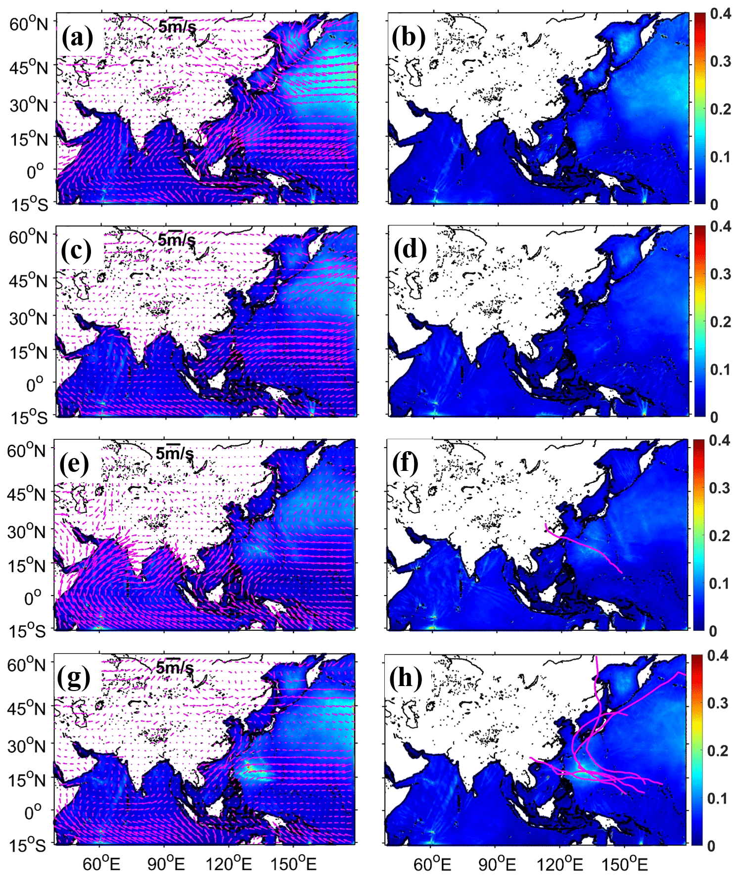
Figure 9 Spatial distributions of SWH RMSDs from WS${}_{\mathrm{multi}\mathrm{3}}^{\mathrm{utms}}$ (a, c, e, g) and WS${}_{\mathrm{multi}\mathrm{3}\left(\mathrm{new}\right)}^{\mathrm{utms}}$ (b, d, f, h) in boreal winter (a, b), spring (c, d), summer (e, f), and autumn (g, h) of 2018 (unit: m). The reference WS${}_{\mathrm{0.125}}^{\mathrm{ut}}$ is used to calculate SWH RMSDs by linear interpolation. The magenta arrows in the left panels (a, c, e, g) are the average wind vectors in every season (unit: m s⁻¹). In panels (f) and (h), the locations of large simulation differences coincide with partial tracks of some typhoons, which are shown with magenta lines.

4.2 Evaluation of the influences of strong wind

Atmospheric wind is an important energy source for ocean surface waves (e.g., Roland and Ardhuin, 2014), and its seasonal characteristics affect the evolution of wave states. Here we use the reference and control experiments to evaluate the influences of strong wind. The former uses an unstructured triangular grid with 0.125^∘ resolutions in the whole domain (named WS${}_{\mathrm{0.125}}^{\mathrm{ut}}$ in Table 1), and the latter uses an unstructured triangular multiscale grid with a varying resolution (0.125, 0.5, and 1^∘) in the study areas (named WS${}_{\mathrm{multi}\mathrm{3}}^{\mathrm{utms}}$ in Table 1). These two experiments share the same shorelines and grid resolution in shallow-water areas, but the control experiment has a coarser grid resolution in deep-water areas. In this section, two experiments are driven by the same ECMWF ERA5 wind, and the spatial distributions of SWH RMSDs in four seasons are shown in Fig. 9. Compared to the reference WS${}_{\mathrm{0.125}}^{\mathrm{ut}}$, simulation differences in WS${}_{\mathrm{multi}\mathrm{3}}^{\mathrm{utms}}$ are very small in most ocean areas (less than 0.1 m) (left panels), such as the south of the Equator region and the northern Indian Ocean region. However, in the north of the northern Pacific Ocean, there are obvious differences in all seasons, especially in boreal winter (more than 0.15 m), as shown in Fig. 9a. Similar visible differences can also be found in the west of the northern Pacific Ocean in autumn (Fig. 9g and h). Wind distributions in this area (magenta arrows in the left panels of Fig. 9) show that the north and west of the northern Pacific Ocean are affected by strong wind, which is westerly wind and tropical cyclones, respectively. We know that when the spatial resolution of wind forcing and wave models is inconsistent, wind signals will be interpolated onto the wave model grid before model integration. Chen et al. (2018) tested the effect of a smoothed wind on wave simulation in an ideal experiment, and the results showed that it reduced the wave energy magnitude. We propose a hypothesis that if the wind is very strong and the wind direction changes rapidly, wind signals will be over-smoothed during the interpolation process (wind forcing with 0.25^∘ resolutions and wave models with 1^∘ resolution), resulting in poor wave simulation accuracy.

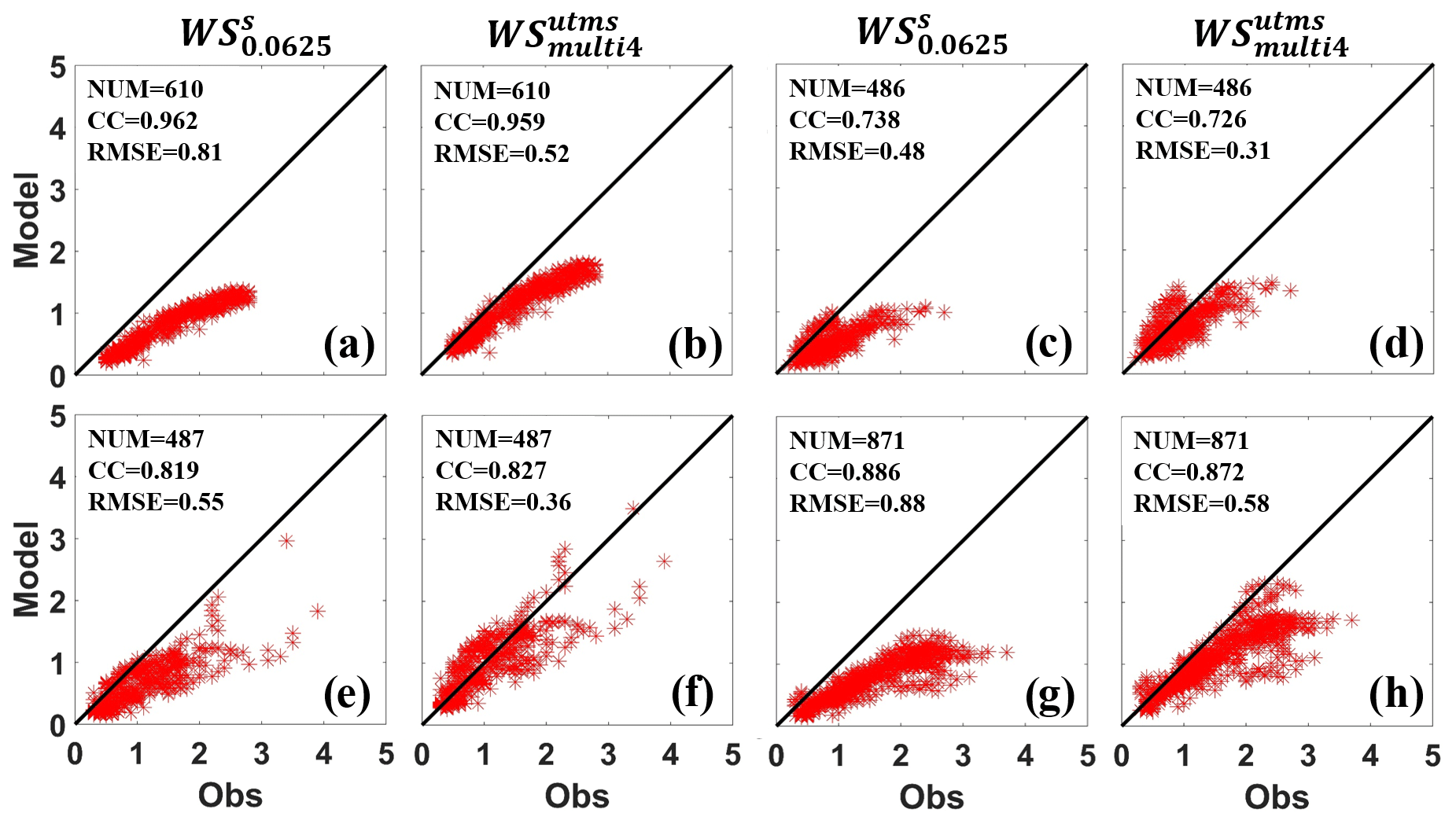
Figure 10 Scattered distributions of SWHs from WS${}_{\mathrm{0.0625}}^{\mathrm{s}}$ (a, c, e, g) and WS${}_{\mathrm{multi}\mathrm{4}}^{\mathrm{utms}}$ (b, d, f, h) at the observational station BSG (marked with yellow stars in Figs. 6 and 7) in boreal winter (a, b), spring (c, d), summer (e, f), and autumn (g, h) of 2018 (unit: m). The black lines in every panel indicate the best fit between wave simulation results (the vertical axis) and observations (the horizontal axis). The number of valid observations and the calculated SWH root mean square errors (RMSEs) and CCs are listed in the upper-left corner of every panel.

To confirm this hypothesis, we encrypt the unstructured triangular multiscale grid in the north of the northern Pacific Ocean for a preliminary test. As shown in Fig. 7, keeping other areas unchanged, we divide the northern Pacific Ocean areas filled with grey (surrounded by a solid blue line) into two small areas named Area1 and Area2, delineated with a dashed cyan line (located at 27^∘ N). Only the mesh resolution in Area1 is changed from 1 to 0.5^∘, and the mesh setting in Area2 remains the same as before. Now, the optimized unstructured triangular multiscale grid is generated. Using this grid, a similar numerical simulation (named WS${}_{\mathrm{multi}\mathrm{3}\left(\mathrm{new}\right)}^{\mathrm{utms}}$ in Table 1) is done. We can see that its simulation differences in the northern Pacific Ocean are largely mitigated (less than 0.1 m) (right panels of Fig. 9) compared with WS${}_{\mathrm{multi}\mathrm{3}}^{\mathrm{utms}}$ (left panels of Fig. 9), while there are still some visible differences in boreal winter (Fig. 9b). We know compared with other seasons that the wind in this season is stronger and changes faster. This situation will lead to over-smoothing wind energy when the wind forcing is interpolated onto wave models' grid and a larger splitting error when the WW3 wave model uses an explicit scheme (CRD-N used here) (Roland, 2009). Splitting errors occur because of a fluctuation splitting scheme used for the integration of geographical, spectral advection terms and source terms. Chen et al. (2018) mitigated the splitting error by using small time steps but with little effect. If using the implicit N scheme, WW3 integrates the wave action equation directly without a splitting error (Abdolali et al., 2020; Sikiric et al., 2018), resulting in slightly smaller simulation differences than that using the explicit CRD-N scheme. Simulation differences in MWD and MWP are also alleviated. As their differences are small, the improvement is not as obvious as SWH (not shown). In terms of computational efficiency, WS${}_{\mathrm{multi}\mathrm{3}\left(\mathrm{new}\right)}^{\mathrm{utms}}$ has only a slightly larger number of grids than WS${}_{\mathrm{multi}\mathrm{3}}^{\mathrm{utms}}$ (Table 1); these two experiments take almost the same computational time (Fig. 13).

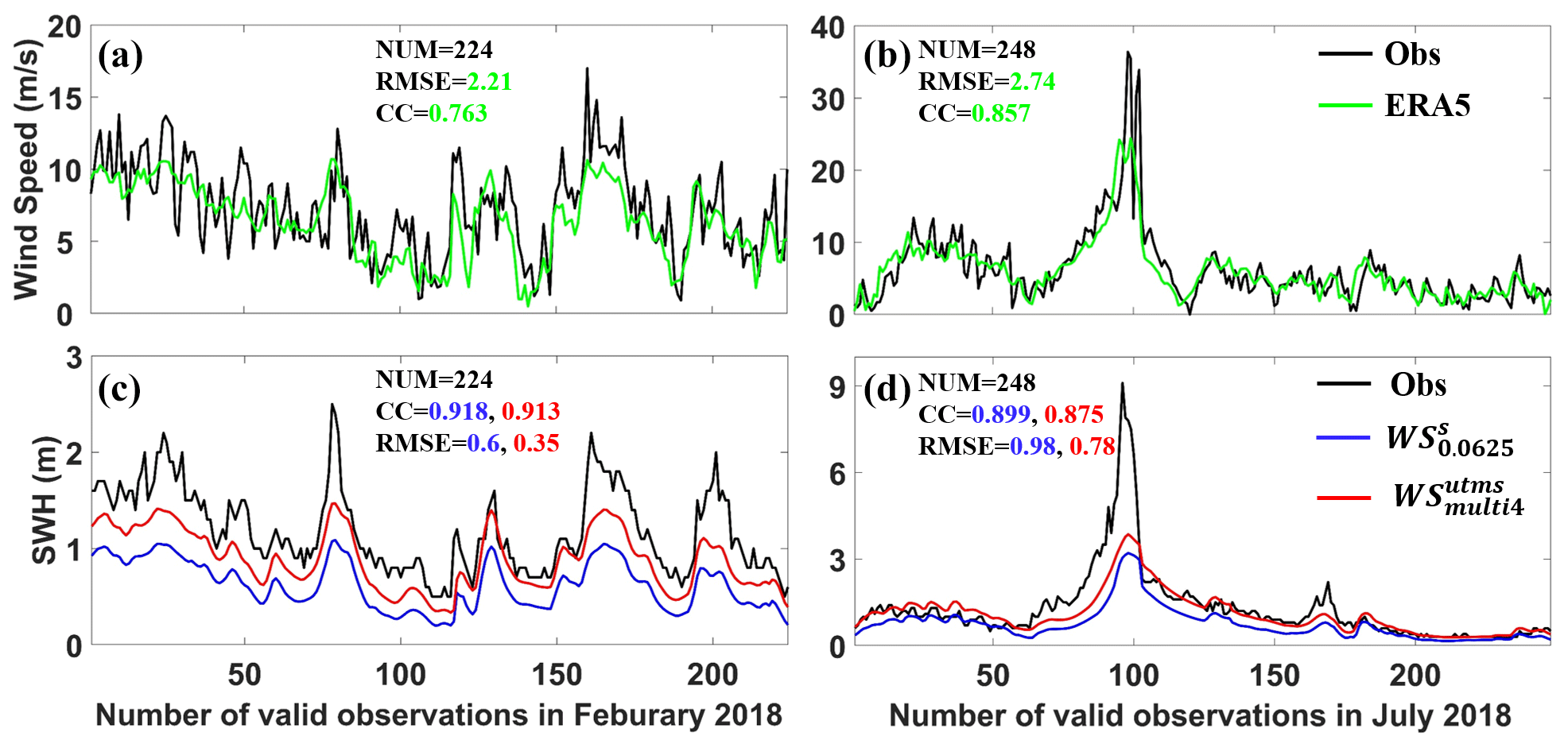
Figure 11 Time series of wind speeds (a, b) and SWHs (c, d) at the BSG observation station in boreal February (a, c) and July (b, d), 2018 (unit: m for SWHs and m s⁻¹ for wind speeds). The observed wind speeds and SWHs are plotted with black lines. The wind forcing is from the ERA5 reanalysis dataset plotted with green lines in (a) and (b). The simulated SWHs from WS${}_{\mathrm{0.0625}}^{\mathrm{s}}$ and WS${}_{\mathrm{multi}\mathrm{4}}^{\mathrm{utms}}$ are plotted with blue and red lines in (c) and (d), respectively.

Different tropical cyclones vary greatly in time, space, and intensity, which will have important effects on wave simulation accuracy. As shown in Fig. 9f and h, locations of large simulation differences overlap the partial tracks of some typhoons (magenta lines). The simulated SWH differences both have a high correlation with wind intensity in active typhoon areas. The large differences often occur when the wind speed exceeds 50 m s⁻¹. Xu et al. (2017) stated that if the wind signal is not enriched from coarse grid to fine grid, only an encrypting wave model resolution has little effect on wave simulation accuracy. The wind forcing we used is from the ECMWF ERA5 reanalysis dataset with a coarse spatial resolution (0.25^∘ lat $\times \mathrm{0.25}{}^{\circ }$ long). It is unable to reproduce the typhoon process well, resulting in underestimated wave simulation results (as shown in Fig. 11b and d) (Hsiao et al., 2020; Jiang et al., 2022; Wu et al., 2020). We preliminarily suggest that the grid resolution in whole active typhoon areas is consistent with the spatial resolution of wind forcing to avoid missing wind signals. In the next paper, we will revise this long-duration reanalysis dataset using typhoon parameters to get a more accurate wave state, analyze the relationship between large simulation differences and typhoon intensity, and then determine the specific area of multiscale grid encryption to further improve simulation efficiency.

In short, in deep-water areas, wave simulation using coarse-resolution grids can achieve the goal of enhancing computational efficiency without sacrificing simulation accuracy. According to the wind intensity, some suggestions are given for designing unstructured multiscale grid systems in these areas. (1) In active typhoon areas, we preliminarily suggest the spatial resolution of multiscale grid systems to be consistent with that of wind forcing to accurately capture the rapidly changing wind characteristics. (2) In the westerly zone, such as 30–60^∘ N areas, the spatial resolution of multiscale grid systems could be twice coarser than that of wind forcing to avoid over-smoothing wind signals. (3) In moderate or weak wind areas, the grid resolution of wave models could be 4 times coarser than that of wind forcing to shorten the computational time consumption.

4.3 Evaluation of influences of complex topography

With the advancement of HPC, ultra-high-resolution coupled models have been widely developed to understand air–sea interactions. For example, Li et al. (2020) have developed three versions of coupled models in the Asia–Pacific area, of which the highest-resolution version is a 3 km atmosphere coupled with a 3 km ocean. This coupled system does not currently achieve online wave coupling because a high-resolution wave simulation has low computational efficiency, as we described earlier (Fig. 3). In this section, we focus on evaluating the effect of increasing spatial resolution in coastal areas on wave simulation accuracy and computational efficiency and explore the possibility of using a multiscale grid to achieve efficient and ultra-high-precision wave simulation. Considering that the highest resolution of the unstructured triangular multiscale grid (WS${}_{\mathrm{multi}\mathrm{3}\left(\mathrm{new}\right)}^{\mathrm{utms}}$) designed above in these areas is 0.125^∘ (about 13 km), we encrypt the grid resolution in coastal areas around the South China Sea (framed by a solid cyan box in Fig. 7) for further testing. The steps are as follows: (1) designing the shorelines with 0.0625^∘ resolutions (about 7 km), (2) adjusting new control lines with 0.125^∘ resolutions in suitable locations, (3) generating the new meshes in shallow-water areas, and (4) replacing these meshes in the previous version (WS${}_{\mathrm{multi}\mathrm{3}\left(\mathrm{new}\right)}^{\mathrm{utms}}$). Now, a finer unstructured triangular multiscale grid is finished (not shown). Afterwards, a similar numerical experiment using the finer unstructured triangular multiscale grid is done, named WS${}_{\mathrm{multi}\mathrm{4}}^{\mathrm{utms}}$ in Table 1.

Similar to the last section, we still design the reference experiment using a structured grid with 0.0625^∘ resolutions in the whole domain (named WS${}_{\mathrm{0.0625}}^{\mathrm{s}}$ in Table 1) to evaluate the performance of this control experiment (WS${}_{\mathrm{multi}\mathrm{4}}^{\mathrm{utms}}$). Since the meshes are modified only in shallow-water areas, we use observation data from three Chinese oceanic stations named BSG (marked with yellow stars in Figs. 6 and 7), DSN, and ZLG (marked with yellow stars in Fig. 7) to evaluate simulation results of the control and reference. Figure 10 shows the scatter diagram of the observed and simulated SWHs at the BSG station within the valid observed time in four seasons of 2018. As described in Sect. 3.1.2, wave simulation using a structured grid over-blocks wave energy at station BSG, resulting in the SWH underestimation. This situation is still not alleviated when the spatial resolution is increased from 0.125^∘ (Fig. 6c) to 0.0625^∘ (Fig. 10a, c, e, g). The WS${}_{\mathrm{multi}\mathrm{4}}^{\mathrm{utms}}$ without considering the island's blocking effect has a good performance (Fig. 10b, d, f, h). The SWH root mean square errors (RMSEs) are reduced by about 35 % in every season.

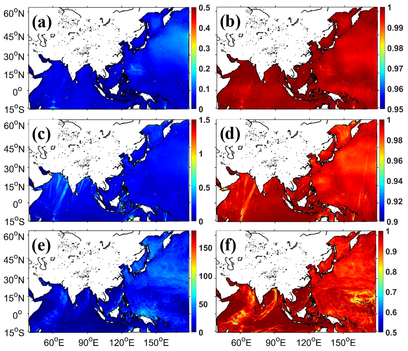
Figure 12 Spatial distributions of RMSDs (a, c, e) and CCs (b, d, f) of SWHs (a, b), MWPs (c, d), and MWDs (e, f) from WS${}_{\mathrm{multi}\mathrm{4}}^{\mathrm{utms}}$ in 2018 (units: panel a, m; panel c, s; panel e, ^∘). WS${}_{\mathrm{0.125}}^{\mathrm{ut}}$ in Table 1 is considered to be a reference to calculate the RMSDs and CCs by linear interpolation.

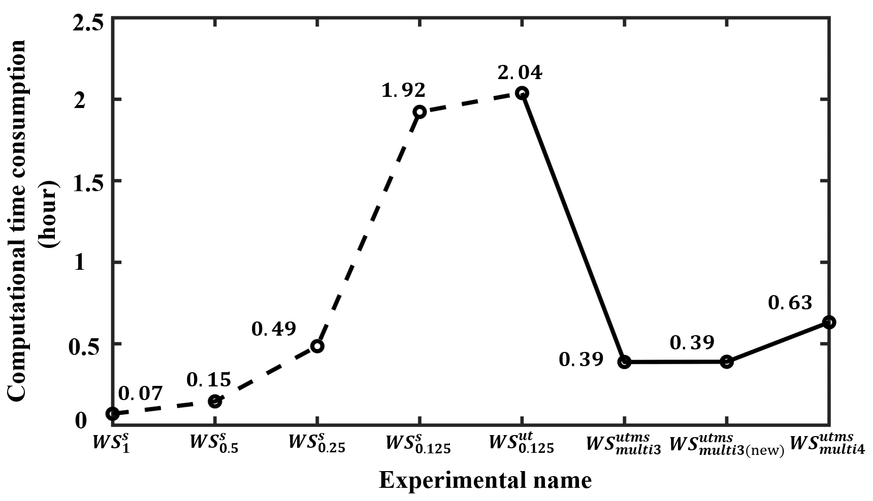
Figure 13 The computational time consumption from wave simulation with unstructured triangular (multiscale) grid systems (solid lines) under the same computational condition. The computational time consumption from Fig. 3 is plotted here with dashed lines for comparison.

We further analyze the temporal evolution of observed and simulated wind speeds and SWHs at the BSG station in February and July 2018 (an example of boreal winter and summer), respectively. As we expected, the observed wind intensity and SWH magnitude have a good agreement, both plotted with black lines in Fig. 11. When the wind is strong, SWH is large, more obviously in July (Fig. 11b and d). Figure 11 also shows the simulated SWHs driven by the same reanalysis wind, plotted with colored lines. It is noted that the ECMWF ERA5 dataset has no reanalysis data available at this station because its spatial resolution is too coarse to identify this station. Simulation results using the multiscale grid (red lines) and structured grid (blue lines) have a similar evolution, but the former is closer to the observation (black lines), whether under low–moderate wind speeds (Fig. 11c) or high wind speeds as the typhoon passes through (typhoon Maria in Fig. 11d). In terms of computational efficiency, WS${}_{\mathrm{multi}\mathrm{4}}^{\mathrm{utms}}$ (0.63 h in Fig. 13) takes much less computational time than WS${}_{\mathrm{0.0625}}^{\mathrm{s}}$ (33.79 h in Fig. 3). Therefore, in shallow-water areas (with a water depth greater than 10 m), wave simulation using the unstructured multiscale grid can improve the description of complex shorelines and topography and enhance wave simulation precision. Similar to the BSG station, the performance of the control and reference experiments at the DSN and ZLG stations are also evaluated. However, because the water depth at these two stations is too shallow (less than 10 m, in Table 2), the WW3 wave model using these two grids has similar underestimated behavior (not shown). This underestimation also occurs even though the wind magnitude and evolution from ECMWF ERA5 are similar to those from the observation (although under this circumstance, the wave simulation using a multiscale grid is closer to the observation than that using a structured grid) (Fig. 11a and c). This indicates that it is urgent to enhance the simulated ability of wave models in shallow-water areas.

Table 3 The performance of WS${}_{\mathrm{multi}\mathrm{3}}^{\mathrm{utms}}$ and the reference WS${}_{\mathrm{0.125}}^{\mathrm{ut}}$, both using four propagation schemes in January 2018.

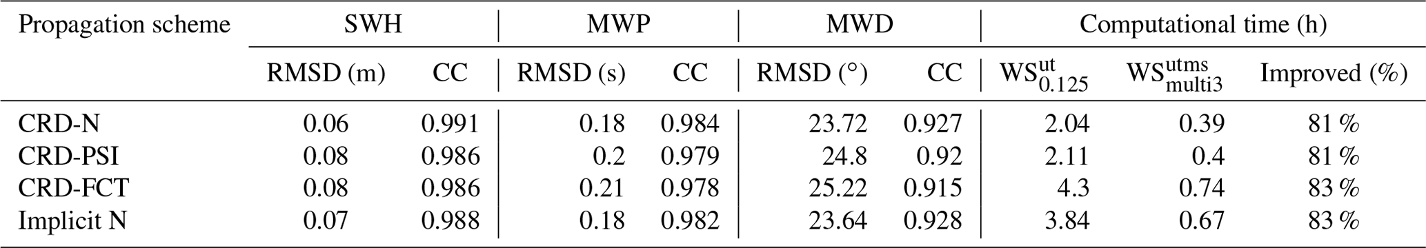
Note: simulation results of ${\mathrm{WS}}_{\mathrm{multi}\mathrm{3}}^{\mathrm{utms}}$ are interpolated onto the reference grid to calculate the RMSDs and correlation coefficients (CCs) of SWH, the mean wave period (MWP) and the mean wave direction (MWD), respectively.

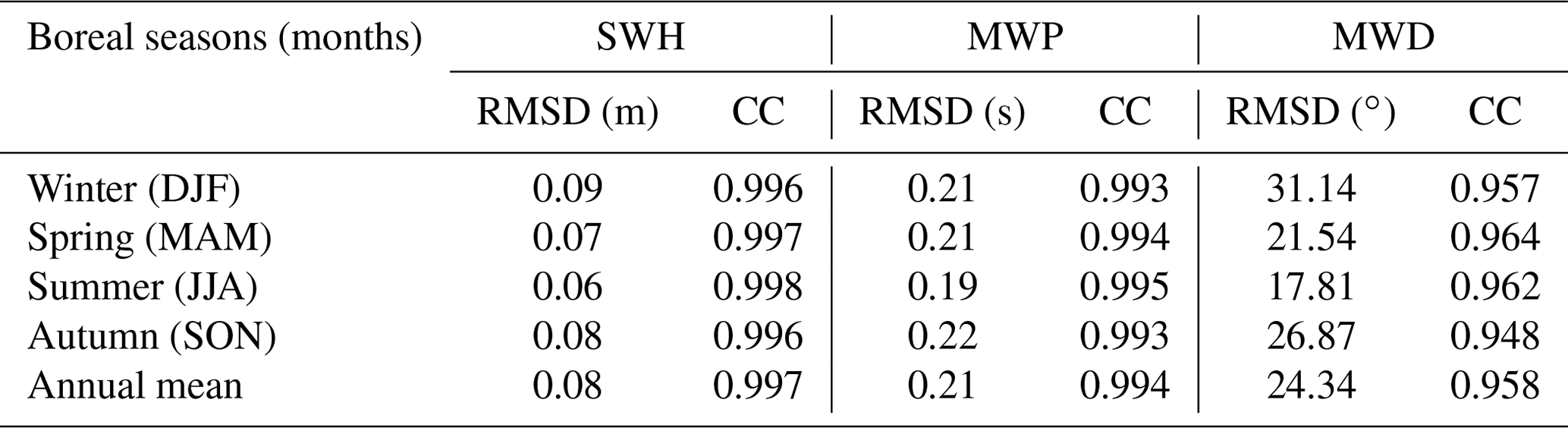
Table 4 The RMSD and CC statistics of SWHs, MWPs, and MWDs from ${\mathrm{WS}}_{\mathrm{multi}\mathrm{4}}^{\mathrm{utms}}$ compared with the reference ${\mathrm{WS}}_{\mathrm{0.125}}^{\mathrm{ut}}$ in 2018.

4.4 Evaluation of the applicability

Through the systematic tests above, we know that the WW3 wave model with a multiscale grid system is feasible and has a good performance in simulation accuracy and computational efficiency. Here, we continue to test its applicability based on the previous section. Since there are a few meshes with 0.0625^∘ resolutions in WS${}_{\mathrm{multi}\mathrm{4}}^{\mathrm{utms}}$, we still use WS${}_{\mathrm{0.125}}^{\mathrm{ut}}$ as the reference to evaluate the performance of this control experiment (WS${}_{\mathrm{multi}\mathrm{4}}^{\mathrm{utms}}$). Figure 12 shows that the two simulation results have negligible differences in 2018. In detail, the RMSDs of SWHs, MWPs, and MWDs are all less than 0.1 m, 0.23 s, and 32^∘ in Table 4, respectively. The CCs of SWHs and MWPs are around 0.99, and the MWD CCs are around 0.95. There is a slight impact on MWD. A similar phenomenon can also be seen in Pallares et al. (2017), where the MWD is the most sensitive among these three variables when the grid used is changed. The control has fewer water points (WS${}_{\mathrm{multi}\mathrm{4}}^{\mathrm{utms}}$, 108, 137 in Table 1), 79 % and 83 % less than the reference using an unstructured triangular grid with 0.125^∘ resolutions (WS${}_{\mathrm{0.125}}^{\mathrm{ut}}$, 521, 911) and the traditional simulation using a structured grid with 0.0625^∘ resolution (WS${}_{\mathrm{0.0625}}^{\mathrm{s}}$, 1, 632, 638) in the whole domain, respectively. Then, WS${}_{\mathrm{multi}\mathrm{4}}^{\mathrm{utms}}$ takes 0.63 h (Fig. 13), saving about 70 % and 98 % of the calculation time compared to the reference WS${}_{\mathrm{0.125}}^{\mathrm{ut}}$ (2.04 h in Fig. 13) and the traditional simulation WS${}_{\mathrm{0.0625}}^{\mathrm{s}}$ (33.79 h in Fig. 3), respectively, when using the same computational resources (128 computing cores) and simulating the same time length (31 d). These results demonstrate that the WW3 wave model using a coarse-resolution grid in deep-water areas has a negligible effect on wave simulation accuracy in the annual mean, and it takes a small fraction of the computational time, compared with that using an unstructured grid or a structured grid with a uniform fine resolution in the whole domain.

From the above detailed evaluation, we can conclude that a new wave modeling framework with a multiscale grid system can achieve the goals of less computational time consumption (Figs. 3 and 13) and better wave simulation precision (Figs. 10, 11, and 12). Such efficient wave simulations are beneficial to operational wave forecasting. It can give faster warnings than before (wave prediction using a uniform fine resolution grid) to minimize the losses of coastal residents when catastrophic waves occur. It can also reduce the error generation and propagation caused by the boundary downscaling process, decrease complexity (compared with a multi-layer nesting simulation), and enhance the computation efficiency of wave components in atmosphere–ocean–wave coupled models. This indicates that this new wave modeling framework will accelerate the pace of high-resolution Earth system models including ocean surface waves as a fast-response physical process at the air–sea interface.

5 Summary and discussions

This paper directly demonstrates that higher-resolution wave simulation can obtain a more accurate wave state, but it requires huge computational resources and has low computing efficiency. To address this situation, this paper designs a new wave modeling framework with a multiscale system. It has the following advantages.

1. Minimizing the number of computational grids. The wave dispersion relation regulating the wave modeling process shows that ocean surface waves are sensitive (insensitive) to topographic effects in shallow-water (deep-water) areas. As a result, the relationship between water depth and half of the wavelength can be a criterion dividing shallow- and deep-water areas, which can decrease the number of fine (coarse) grids in shallow-water (deep-water) areas as much as possible. This is more advantageous when the ocean wave process is incorporated into Earth system models because it can shorten the added computational time considerably.

2. Quantifying the match between grid resolution settings and wind signals. After a series of experiment evaluations, this paper gives some suggestions for designing unstructured multiscale grid systems in deep-water areas to avoid over-smoothing wind signals and enhance computational efficiency. In active typhoon areas, westerly areas, and weak wind areas, the spatial resolution of multiscale grid systems is suggested to be 1, 2, and 4 times coarser than that of wind forcing, respectively.

3. Having similar accuracy using different spatial propagation schemes. This wave modeling framework has a variable grid resolution in geographic space. The performance of wave simulation using four propagation schemes (including CRD-N, CRD-PSI, CRD-FCT, and implicit N) in this space is evaluated. Results show that the four schemes have similar behavior in simulation accuracy, but the default CRD-N scheme takes the least computational time.

4. Achieving efficient and high-precision wave simulation. Evaluations of a series of experiments show that the designed wave modeling framework can achieve the goals of enhancing wave simulation precision and saving computational costs. Compared with using an unstructured grid (WS${}_{\mathrm{0.125}}^{\mathrm{ut}}$, 0.125^∘ in the whole domain), the wave model using the unstructured multiscale grid (WS${}_{\mathrm{multi}\mathrm{3}}^{\mathrm{utms}}$, keeping the same resolution (0.125^∘) in shallow-water areas and varying the resolution (0.5^∘ and 1^∘) in deep-water areas) has very similar performance in simulation accuracy but decreases more than 80% of the computational time consumption. Compared with using a structured grid (WS${}_{\mathrm{0.0625}}^{\mathrm{s}}$, 0.0625^∘ in the whole domain), the wave model using the multiscale grid (WS${}_{\mathrm{multi}\mathrm{4}}^{\mathrm{utms}}$, keeping the same resolution (0.0625^∘) in the South China Sea area and varying the resolution (0.125, 0.5, and 1^∘) in other areas) can obtain more accurate wave states and only takes 2 % of the computational time.

After establishing this powerful wave modeling framework, we will continue to conduct the following studies in the future.

1. This framework can be updated constantly in order to do the following.

   • a.

     Optimize multiscale grids. As HPC technology advances, a multiscale grid with ultra-high-resolution (tens of meters or even meters) in coastal areas and gradually coarse resolution towards the open ocean, eventually covering the global ocean, is needed. A very flexible and automatic tool, OceanMesh2D (Roberts et al., 2019), is used to generate this multiscale grid, which does not take much time. In the process of grid generation, a quantitative relationship of spatial resolution between wind forcing and wave models is provided in this paper for reference.

   • b.

     Further improve the computational efficiency. A powerful implicit scheme is recommended because it is not restrained by the CFL condition compared with the commonly used explicit scheme. We can set relatively large and reasonable integration time steps to further save computational time. Moreover, the newly developed parallelization algorithm named domain decomposition (Abdolali et al. 2020) can greatly reduce the number of information exchanges between computing cores compared with the old algorithm called card deck.

   • c.

     Improve physical processes. The physical processes in current wave models are suitable for wave simulation on the scale of hundreds of meters or kilometers. It is urgent to improve the underestimated wave states in coastal areas in numerical simulation and develop physical processes to enhance the simulation ability of wave models with the scale of tens of meters or even meters. In particular, the physical mechanism and numerical scheme of wave models using multiscale grids, which is the mainstream, should be improved.

   • d.

     Optimize the interpolation method. A linear interpolation method in wave models is used to address the common phenomenon that the spatial resolution of wave models and external forcings is inconsistent. This will over-smooth wind energy, leading to underestimated wave energy and poor wave simulation accuracy. A more reasonable interpolation method should then be explored to alleviate this situation.

2. The applicability of this framework will be validated further.

   • a.

     Validation using other wind forcings. The ECMWF ERA5 atmospheric reanalysis dataset is used to drive the WW3 wave model with a multiscale grid in this paper. The applicability of this framework should be further verified using another common wind forcing, the Climate Forecast System Version 2 (CFSR2) from the National Centers for Environmental Prediction (NCEP) with 0.2^∘ resolutions. Moreover, the wind from an ultra-high-resolution coupled system which has the ability to describe the track and intensity of tropical cyclones should be used to verify the applicability of this framework in active typhoon areas.

   • b.

     Validation in the Simulating WAves Nearshore (SWAN) wave model. This paper systematically evaluates the framework in the WW3 wave model. Since the SWAN wave model has similar modeling ideas and governing equations to the WW3 wave model, the quantitative relationship of spatial resolution between wave models and wind forcing obtained in WW3 is also theoretically applicable to SWAN. More detailed testing and evaluations will be done in the future. It should be noted that this framework is not suitable for the WAve Modeling (WAM) wave model, for this model does not currently support unstructured triangular grids.

   • c.

     Validation in Earth system models. As an important physical process at the air–sea interface, ocean surface waves should be incorporated into Earth system models. Usually, the significant wave feedback to the atmosphere and ocean is where the wave height is large, and these areas are already gridded with high-resolution model resolutions in this paper. A more detailed test of whether the wave feedback to air–sea interactions is related to wave model resolutions that have inhomogeneous wave information will be conducted further. Afterwards, a systematic evaluation of the contribution of ocean surface waves to the atmospheric planetary boundary layer and upper-ocean mixing will be carried out. This will help us to deepen our understanding of physical processes at the air–sea interface.