The capabilities of the adjoint of GEOS-Chem model to support HEMCO emission inventories and MERRA-2 meteorological data

The adjoint of the GEOS-Chem (Goddard Earth Observing System with Chemistry) model has been widely used to constrain the sources of atmospheric compositions. Here, we designed a new framework to facilitate emission inventory updates in the adjoint of the GEOS-Chem model. The major advantage of this new framework is good readability and extensibility, which allows us to support Harmonized Emissions Component (HEMCO) emission inventories conveniently and to easily add more emission inventories following future updates in GEOS-Chem forward simulations. Furthermore, we developed new modules to support MERRA-2 (Modern-Era Retrospective Analysis for Research and Applications, version 2) meteorological data, which allows us to perform long-term analyses with consistent meteorological data for the period 1979–present. The performances of the developed capabilities were evaluated with the following steps: (1) diagnostic outputs of carbon monoxide (CO) sources and sinks to ensure the correct reading and use of emission inventories, (2) forward simulations to compare the modeled surface and column CO concentrations among various model versions, (3) backward simulations to compare adjoint gradients of global CO concentrations to CO emissions with finite-difference gradients, and (4) observing system simulation experiments (OSSEs) to evaluate the model performance in 4D variational (4D-Var) assimilations. Finally, an example application of 4D-Var assimilation was presented to constrain anthropogenic CO emissions in 2015 by assimilating Measurement of Pollution in the Troposphere (MOPITT) CO observations. The capabilities developed in this work are important for better applications of the adjoint of the GEOS-Chem model in the future. These capabilities will be submitted to the standard GEOS-Chem adjoint code base for better development of the community of the adjoint of the GEOS-Chem model.

1 Introduction

The Goddard Earth Observing System with Chemistry (GEOS-Chem) model is a global 3D chemical transport model (CTM) and has been widely used to analyze the sources and variabilities of atmospheric compositions (Whaley et al., 2015; Li et al., 2019; Hammer et al., 2020; Jiang et al., 2022). The GEOS-Chem model is driven by meteorological reanalysis data from the Goddard Earth Observing System (GEOS) of the Global Modeling and Assimilation Office (GMAO). Emissions in the GEOS-Chem model are calculated with state-of-the-art inventories such as CEDS (Community Emissions Data System) (Hoesly et al., 2018), MIX (Li et al., 2017) and NEI2011 (National Emissions Inventory). Based on the GEOS-Chem forward simulation, the adjoint of the GEOS-Chem model (Henze et al., 2007) further provides the capability for backward simulation of physical and chemical processes within the 4D variational (4D-Var) framework. The major advantage of the adjoint model is obtaining the sensitivity of atmospheric concentrations to multiple model variables within a single backward simulation. The major applications of the adjoint of the GEOS-Chem model include inverse analyses of atmospheric composition emissions by minimizing the difference between simulations and observations (Jiang et al., 2015a; Zhang et al., 2018; Qu et al., 2022), as well as sensitivity analyses to analyze the sources of atmospheric compositions (Jiang et al., 2015b; Zhao et al., 2019; Dedoussi et al., 2020).

The algorithm of the 4D-Var framework requires identical model processes in the forward and backward simulations. Ideally, the code for the adjoint model should be updated following the GEOS-Chem forward codes to take advantage of the new features in GEOS-Chem forward simulations. However, the updates in the adjoint model are difficult and usually delayed. For example, the MERRA-2 (Modern-Era Retrospective Analysis for Research and Applications, version 2) meteorological reanalysis data with temporal coverage of 1979–present were supported in the GEOS-Chem forward simulations in v11-01. The adjoint of the GEOS-Chem model does not support MERRA-2, and thus, long-term analysis must combine different meteorological reanalysis data, such as GEOS-4 (1985–2007), GEOS-5 (2004–2012) and GEOS-FP (2012–present). For instance, Jiang et al. (2017) constrained global carbon monoxide (CO) emissions in 2001–2015, while the derived trends in CO emissions in Jiang et al. (2017) could be affected by the discontinuity among various versions of the meteorological data (i.e., GEOS-4 in 2001–2003, GEOS-5 in 2004–2012 and GEOS-FP in 2013–2015) and the lack of consistency in the model physics of GEOS-5.

Emission inventories play a key role in the simulation of atmospheric compositions. The Harmonized Emissions Component (HEMCO) (Keller et al., 2014; Lin et al., 2021) was included in the GEOS-Chem forward simulations in v10-01. HEMCO is responsible for inputs of meteorological and emission data with default support for emission inventories such as CEDS, MIX and NEI2011. New emission inventories can be added readily within the HEMCO framework. There are noticeable differences between HEMCO and the adjoint of the GEOS-Chem model. First, meteorological and emission data are read with individual modules in the adjoint of the GEOS-Chem model. Second, the inputs of emission inventories are undertaken by different modules that were developed individually with significant discrepancies in the source code. In addition, the file format (e.g., binary punch in the adjoint of GEOS-Chem that is the format of older GEOS-Chem versions in contrast to netCDF in HEMCO), the emission variables and the usage methods of emission variables (e.g., emission hierarchy, scaling factors and time slice) are inconsistent. These differences have posed a barrier to the application of new emission inventories in the adjoint of the GEOS-Chem model.

The lack of support to the updated emission inventories can affect the applications of the adjoint of the GEOS-Chem model. First, adjoint-based sensitivity analyses are obtained by the backward simulations of atmospheric compositions (i.e., adjoint tracers) and the combination of adjoint tracers with emissions. Out-of-date emission inventories can thus result in inaccurate estimation of the adjoint sensitivities. Second, while inverse analyses are constrained by atmospheric observations, the updated emission inventories are still critical because they are helpful for better convergence of 4D-Var assimilations by setting a more reasonable a priori penalty in the cost function. For instance, the a priori biomass burning CO emissions (GFED3, van der Werf et al., 2010) in Jiang et al. (2017) lack interannual variabilities later than 2011. In order to obtain reasonable convergence of biomass burning emissions, the a priori biomass burning emissions in September–November 2006 were applied to September–November 2015 over Indonesia in Jiang et al. (2017).

Ideally, people should consider porting the complete HEMCO to the adjoint of the GEOS-Chem model to match the new features in GEOS-Chem forward simulations. However, a complete port of HEMCO implies replacing the input framework of the adjoint of the GEOS-Chem model, as well as a restructuring of HEMCO and the adjoint of the GEOS-Chem model to address the compatibility issues, which is very challenging and may not be necessary because the meteorological modules still work well in the adjoint of the GEOS-Chem model. Consequently, a major objective of this work is to design a new framework to facilitate emission inventory updates in the adjoint of the GEOS-Chem model. For this objective, this new framework must have good readability and extensibility to allow us to support HEMCO emission inventories conveniently and to add more emissions inventories following future updates in GEOS-Chem forward simulations easily. Furthermore, we developed new modules to support MERRA-2 meteorological data within the current framework of the adjoint of the GEOS-Chem model as reusing existing frameworks can save much work.

CO is one of the most important atmospheric pollutants and plays a key role in tropospheric chemistry. Sources of atmospheric CO include fossil fuel combustion, biomass burning and oxidation of hydrocarbons. The major sink of atmospheric CO is hydroxyl radical (OH). The simple chemical sink of atmospheric CO allows us to simulate atmospheric CO with linearized chemistry; for example, the tagged-CO mode of the GEOS-Chem model can reduce the calculation cost by 98 % with respect to the full chemistry mode by reading archived monthly OH fields. The tagged-CO mode of the GEOS-Chem model has been widely used to investigate the sources and variabilities of atmospheric CO in recent decades (Heald et al., 2004; Kopacz et al., 2009; Jiang et al., 2017). The capabilities developed in this work are thus based on the tagged-CO mode as it can effectively accelerate the model development process. More efforts are needed in the future to extend these capabilities to support emissions inventories associated with full chemistry simulations.

The results presented in this paper show the development, integration, evaluation and application of these new capabilities, which is important for better applications of the adjoint of the GEOS-Chem model in the future. The capabilities developed in this work will be submitted to the standard GEOS-Chem adjoint code base (Henze et al., 2007) for better development of the community of the adjoint of the GEOS-Chem model. This paper is organized as follows: in Sect. 2, we describe the adjoint of the GEOS-Chem model, the development of these new capabilities and the Measurement of Pollution in the Troposphere (MOPITT) CO observations used in this work. In Sect. 3, we evaluate the performances of the developed capabilities in forward and backward simulations together with observing system simulation experiments (OSSEs) to evaluate the model performance in 4D-Var assimilations. An example application of 4D-Var assimilation to constrain anthropogenic CO emissions in 2015 by assimilating MOPITT CO observations was also presented. Our conclusions follow in Sect. 4.

2 Methodology and data

2.1 Adjoint of the GEOS-Chem model

We use version v35n of the adjoint of the GEOS-Chem model. Our analysis is conducted at a horizontal resolution of $\mathrm{4}{}^{\circ }\times \mathrm{5}{}^{\circ }$ with 47 vertical levels and employs the CO-only simulation (tagged-CO mode). The global default anthropogenic emission inventory in the standard version of the adjoint of the GEOS-Chem model (hereafter referred to as GC-Adjoint-STD) is the Global Emissions InitiAtive (GEIA), but this is replaced by the following regional emission inventories: NEI2008 in North America, the Criteria Air Contaminants (CAC) inventory for Canada, the Big Bend Regional Aerosol and Visibility Observational (BRAVO) Study Emissions Inventory for Mexico (Kuhns et al., 2003), the Cooperative Program for Monitoring and Evaluation of the Long-range Transmission of Air Pollutants in Europe (EMEP) inventory for Europe in 2000 (Vestreng and Klein, 2002) and the INTEX-B Asia emissions inventory for 2006 (Zhang et al., 2009). Biomass burning emissions are based on the GFED3 (van der Werf et al., 2010).

The objective of the 4D-Var approach is to minimize the difference between simulations and observations described by the cost function (Henze et al., 2007):

$$\begin{array}{}\text{(1)}& \begin{array}{rl}J\left(\mathit{x}\right)& ={\sum }_{i=\mathrm{1}}^N\left({\mathbf{F}}_i\right(\mathit{x})-{\mathit{z}}_i{)}^T{\mathbf{S}}_{\mathrm{\Sigma }}^{-\mathrm{1}}({\mathbf{F}}_i\left(\mathit{x}\right)-{\mathit{z}}_i)\\ & +\mathit{\gamma }(\mathit{x}-{\mathit{x}}_a{)}^T{\mathbf{S}}_{\mathrm{a}}^{-\mathrm{1}}(\mathit{x}-{\mathit{x}}_a),\end{array}\end{array}$$

where x is the state vector of CO emissions, N is the number of observations that are distributed in time over the assimilation period, z_i is a given measurement, and F(x) is the forward model. The error estimates are assumed to be Gaussian and are given by S_Σ, the observational error covariance matrix, and S_a, the a priori error covariance matrix. The cost function is minimized through minimizing the adjoint gradients by adjusting the CO emissions iteratively:

$$\begin{array}{}\text{(2)}& \begin{array}{rl}{\mathrm{\nabla }}_{\mathit{x}}J\left(\mathit{x}\right)& ={\sum }_{k=\mathrm{1}}^N\left[\mathrm{2}{\mathbf{S}}_{\mathrm{\Sigma }}^{-\mathrm{1}}\left({\mathbf{F}}_i\right(\mathit{x})-{\mathit{z}}_i){\displaystyle \frac{\partial {\mathbf{F}}_i}{\partial \mathit{x}}}\right]\\ & +\mathrm{2}\mathit{\gamma }{\mathbf{S}}_{\mathrm{a}}^{-\mathrm{1}}(\mathit{x}-{\mathit{x}}_a).\end{array}\end{array}$$

We assume a uniform observation error of 20 %. The combustion CO sources (fossil fuel, biofuel and biomass burning) and the oxidation source from biogenic volatile organic compounds (VOCs) are combined, assuming a 50 % uniform a priori error. We optimize the source of CO from the oxidation of methane (CH₄) separately as an aggregated global source, assuming an a priori uncertainty of 25 %. The CO emission estimates are optimized with monthly temporal resolution. Following Jiang et al. (2017), we performed 40 iterations (forward + backward simulations) for each month, which usually produced six to eight accepted iterations (i.e., successful line searches in the large-scale bound constrained optimization (L-BFGS-B, Zhu et al., 1997)) to reduce the cost functions and adjoint gradients. The a posteriori CO emission estimates were calculated based on the last accepted iteration, which usually corresponded to the iteration with the lowest cost function.

Figure 1 Framework to read the updated emission inventories in GC-Adjoint-HEMCO.

2.2 New framework to read emission inventories

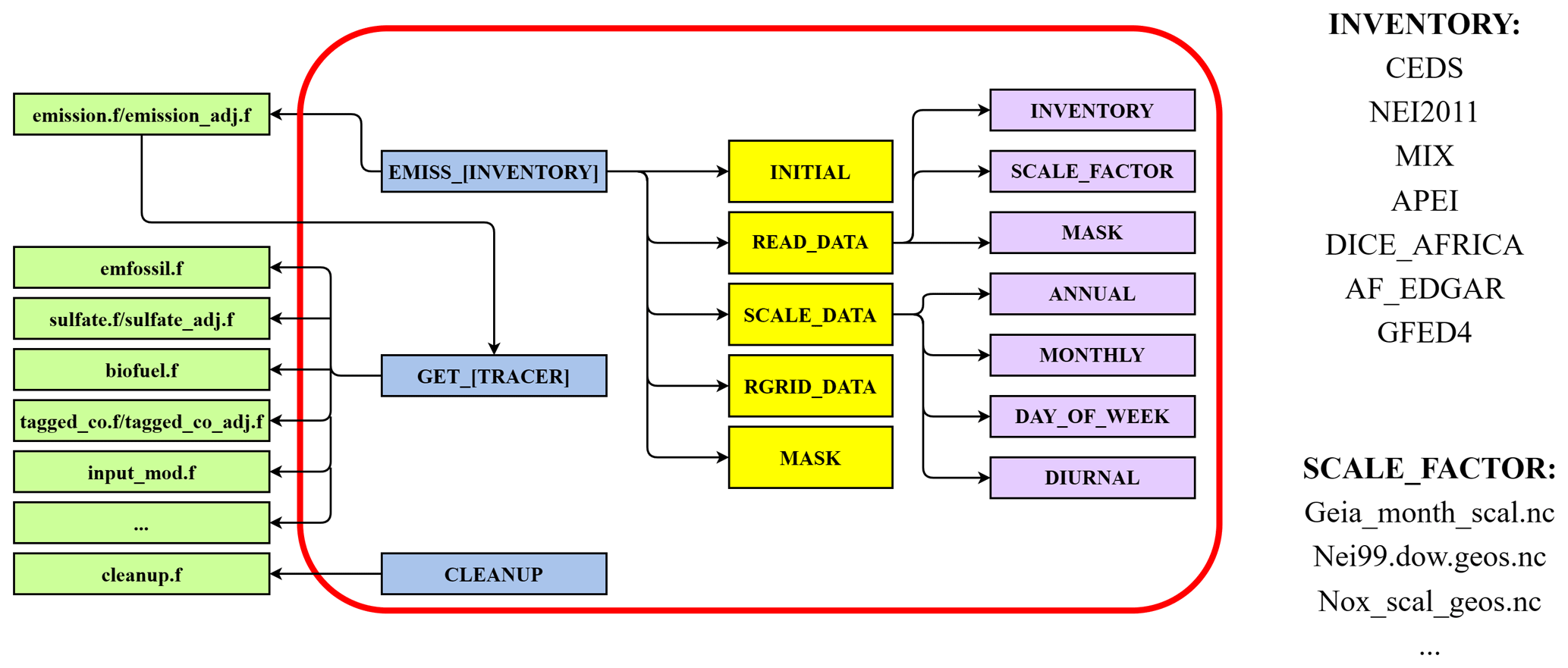
A major objective of this work is to design a new framework to facilitate emission inventory updates in the adjoint of the GEOS-Chem model. As shown in Fig. 1, we first initialize the array in [INITIAL] and batch read the emission data in [READ_DATA], which were interpolated offline with $\mathrm{1}{}^{\circ }\times \mathrm{1}{}^{\circ }$ resolution by considering the mass conservation. Here, the data include the emission inventory data listed in Table S1 in the Supplement, the corresponding scaling factor data and the mask map files of domain definitions. The data are scaled in [SCALE_DATA] by multiplying the corresponding annual, seasonal, monthly, weekly and 24 h emission factors and are then interpolated online to the current resolution ($\mathrm{4}{}^{\circ }\times \mathrm{5}{}^{\circ }$ in this work) of the model by [RGRID_DATA], which was followed by the application of region masks in [MASK].

The emission variable of CO obtained in this part is written to the model memory in emission.f and emission_adj.f by calling DO_EMISSIONS to ensure consistent emissions in both forward and backward simulations. The GET_[TRACER] subroutines are used to obtain the CO emission variable, which participates in the calculation of physicochemical processes in the model, to interact with other modules. Finally, the variable is cleaned from the memory by the [CLEANUP] module. It should be noted that a two-step interpolation is employed in this work (hereafter referred to as GC-Adjoint-HEMCO) following GC-Adjoint-STD, for example, $\mathrm{0.1}{}^{\circ }\times \mathrm{0.1}{}^{\circ }$ to $\mathrm{1}{}^{\circ }\times \mathrm{1}{}^{\circ }$ and then to $\mathrm{4}{}^{\circ }\times \mathrm{5}{}^{\circ }$ for the NEI2011 inventory, which is different from the one-step interpolation in the GEOS-Chem forward model (v12-08-01, hereafter referred to as GC-v12), for example, $\mathrm{0.1}{}^{\circ }\times \mathrm{0.1}{}^{\circ }$ to $\mathrm{4}{}^{\circ }\times \mathrm{5}{}^{\circ }$ directly for the NEI2011 inventory. The different interpolation methods can lead to differences in the interpolated emission data.

Table 1 CO emissions for each inventory in 2015 (in Tg yr⁻¹).

2.3 Updates in emission inventories

In addition to baseline emission data, there are critical factors that affect the usage of emission data in the models. Reading the emission data correctly thus does not necessarily mean using emission data correctly. For example, the emission hierarchy is used to prioritize emission fields within the same emission category. Emissions of a higher hierarchy overwrite lower-hierarchy data. Regional emission inventories usually have a higher hierarchy within their mask boundaries. Scaling factors are used to adjust the baseline emissions with annual, seasonal, monthly, weekly and 24 h temporal scales. The time slice selection is used to define the usage methods of the emission data outside the original temporal range; for instance, data can be interpreted as climatology and recycled once the end of the last time slice is reached, or they can be considered only as long as the simulation time is within the time range. Consequently, we must validate the integrated emissions carefully to ensure that the abovementioned factors have been correctly applied and to ensure that the calculated emissions are reasonable for individual inventories and the combination of all inventories.

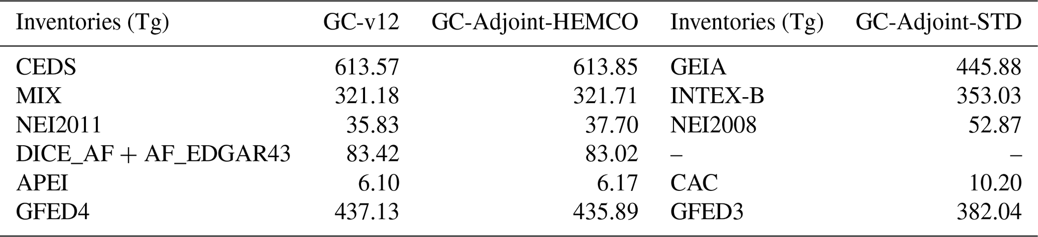
To take advantage of this new framework, six HEMCO emission inventories have been added to this work. To validate the emissions, we performed actual simulations with GC-v12, GC-Adjoint-HEMCO and GC-Adjoint-STD, and the emissions were calculated in the model simulations and then output to the Log file. As shown in Table S1, the CEDS emission inventory ($\mathrm{0.5}{}^{\circ }\times \mathrm{0.5}{}^{\circ }$) is adopted in GC-Adjoint-HEMCO to provide global default emissions for 1750–2019. The diurnal scale factors are applied to obtain CO emissions at different moments of the day. Figure S1 (see the Supplement) shows CEDS CO emissions in 2015 in GC-v12 and GC-Adjoint-HEMCO and GEIA CO emissions in GC-Adjoint-STD, and we find noticeable differences in CO emissions between CEDS and GEIA. As shown in Table 1, the CEDS CO emissions in 2015 were 613.57 and 613.85 Tg yr⁻¹ in GC-v12 and GC-Adjoint-HEMCO, respectively, with a relative difference of 0.05 % between GC-v12 and GC-Adjoint-HEMCO. The GEIA CO emissions in 2015 were 445.88 Tg yr⁻¹ in GC-Adjoint-STD.

The default CEDS inventory is replaced by the following regional emission inventories in GC-Adjoint-HEMCO: MIX in Asia ($\mathrm{0.25}{}^{\circ }\times \mathrm{0.25}{}^{\circ }$), NEI2011 in the United States ($\mathrm{0.1}{}^{\circ }\times \mathrm{0.1}{}^{\circ }$), DICE_AFRICA and EDGARV43 in Africa ($\mathrm{0.1}{}^{\circ }\times \mathrm{0.1}{}^{\circ }$), and APEI in Canada ($\mathrm{0.1}{}^{\circ }\times \mathrm{0.1}{}^{\circ }$). As shown in Fig. S2, the MIX inventory provides Asian emissions in 2008–2010, accompanied by diurnal scale factors to describe daily emission variations. The $\mathrm{1}{}^{\circ }\times \mathrm{1}{}^{\circ }$ scale factors in the AnuualScalar.geos.1x1.nc file further provide the annual variation in 1985–2010. As shown in Table 1, the MIX CO emissions in 2015 were 321.18 and 321.71 Tg yr⁻¹ in GC-v12 and GC-Adjoint-HEMCO, respectively, with a relative difference of 0.17 % between GC-v12 and GC-Adjoint-HEMCO. The INTEX-B CO emissions in 2015 were 353.03 Tg yr⁻¹ in GC-Adjoint-STD.

The NEI2011 inventory (Fig. S3) provides anthropogenic emissions for the United States in 2011 with annual scalar factors from 2006 to 2013. The weekday and weekend factors are read from the NEI99.dow.geos.1x1.nc file from 1999 with CO factors of 1.0 on weekdays and between 0.990 and 0.997 on Saturdays and Sundays. The NEI2011 CO emissions in 2015 were 35.83 and 37.70 Tg yr⁻¹ in GC-v12 and GC-Adjoint-HEMCO, respectively, with a relative difference of 5.22 % between GC-v12 and GC-Adjoint-HEMCO. The NEI2008 CO emissions in 2015 were 52.87 Tg yr⁻¹ in GC-Adjoint-STD. APEI (Fig. S4) is the primary source of anthropogenic emissions in the Canadian domain. The APEI CO emissions in 2015 were 6.10 and 6.17 Tg yr⁻¹ in GC-v12 and GC-Adjoint-HEMCO, respectively, with a relative difference of 1.14 % between GC-v12 and GC-Adjoint-HEMCO. The CAC CO emissions in 2015 were 10.20 Tg yr⁻¹ in GC-Adjoint-STD. Following GC-v12, the CO emissions in APEI are enhanced by 19 % to account for co-emitted VOCs in the tagged-CO simulation.

Emissions for the African domain are provided by the combination of DICE_AFRICA and EDGARV43 (Fig. S5). Here, DICE_AFRICA includes anthropogenic and biofuel emissions in 2013. We read the DICE_AFRICA emissions data into the model in two types according to the guidelines of the inventory. Emissions from sectors such as automobiles and motorcycles are aggregated into anthropogenic sources, and household-generated emissions such as charcoal and agricultural waste are aggregated into biofuel sources. Efficient combustion emissions from EDGAR v4.3 in 1970–2010 then compensate for the lacking sources in DICE_AFRICA. Daily variation factors for CO are also used here for emissions across the African region. The 2010 CO seasonal-scale factors are used in EDGAR v4.3 for sectoral emission sources. The DICE_AFRICA and EDGARV43 CO emissions in 2015 were 83.42 and 83.02 Tg yr⁻¹ in GC-v12 and GC-Adjoint-HEMCO, respectively, with a relative difference of −0.48 % between GC-v12 and GC-Adjoint-HEMCO. Following GC-v12, the CO emissions in DICE_AFRICA and EDGARV43 are enhanced by 19 % to account for co-emitted VOCs in the tagged-CO simulation.

Table 2 Regional combustion CO emissions, VOC-generated CO (PCO_NMVOC), CH₄-generated CO (PCO_CH₄), CO sinks (CO_OH, calculated as CO_OH = KRATE × CO × OH), and simulated surface and column CO concentrations in 2015. The region definitions are shown in Fig. 2a.

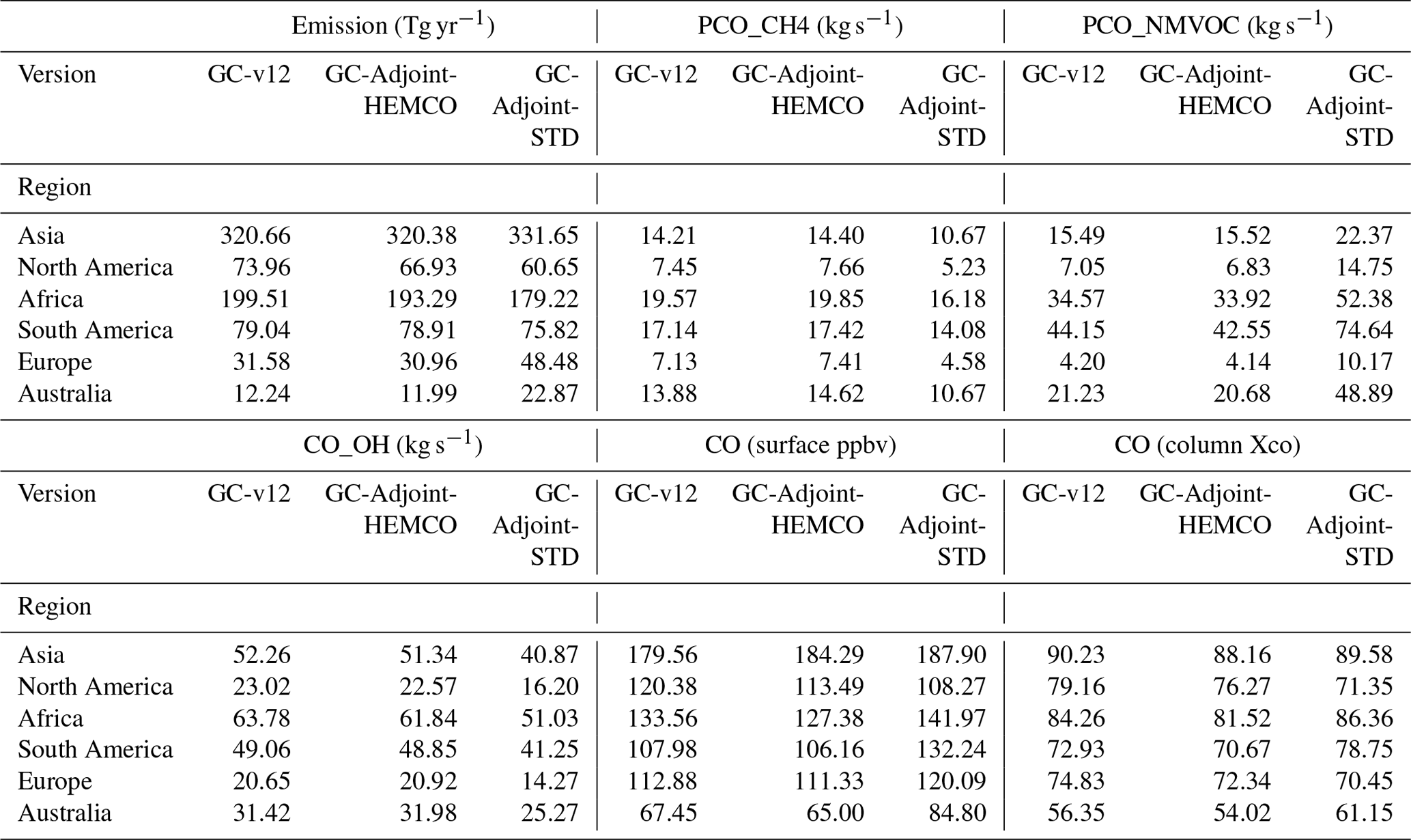
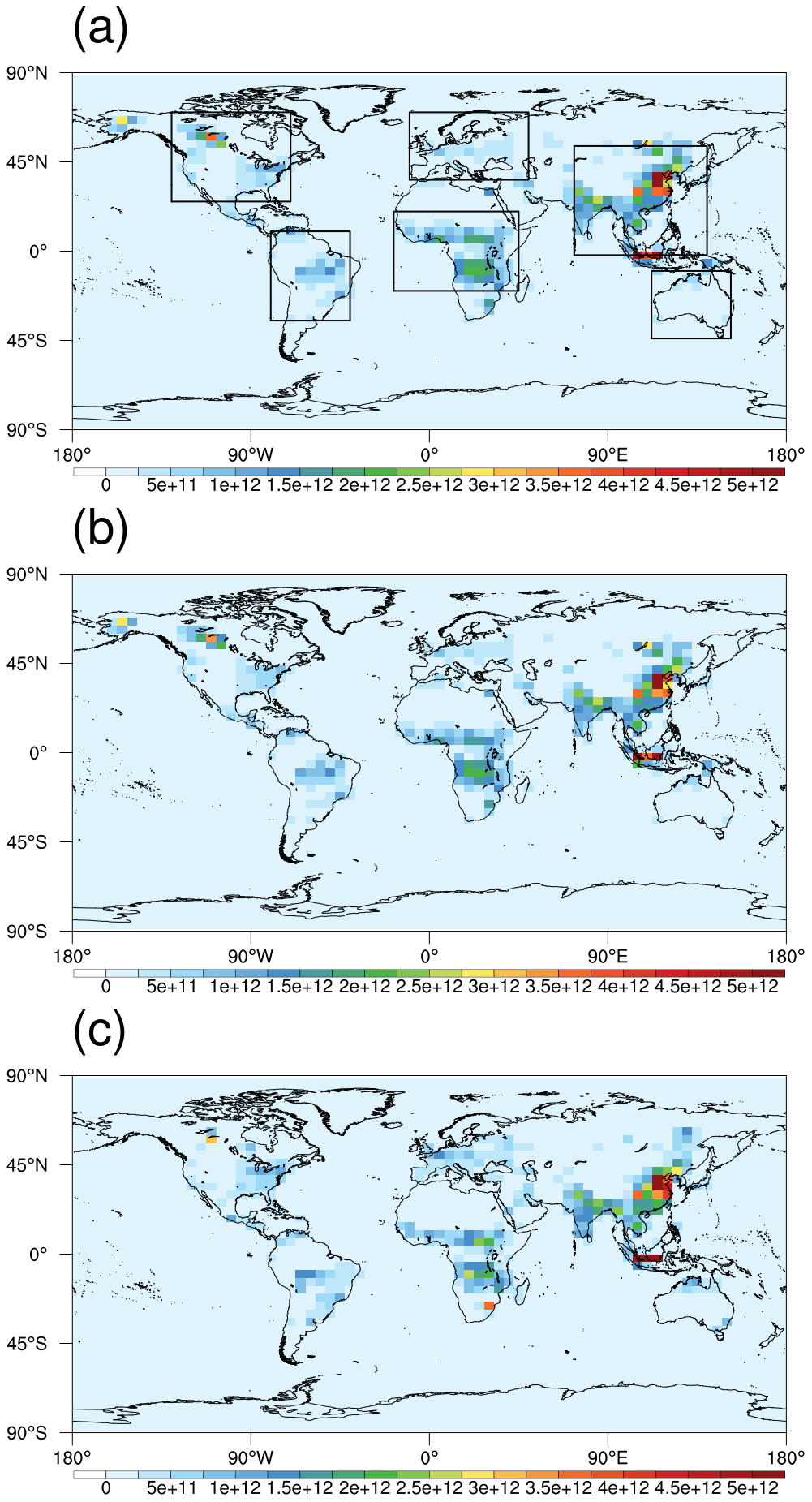
Figure 2 Total combustion CO emissions in 2015 from (a) GC-v12, (b) GC-Adjoint-HEMCO and (c) GC-Adjoint-STD (in molec. cm² s⁻¹).

The biomass burning emission inventory in GC-Adjoint-HEMCO is GFED4 (Fig. S6), which includes dry-matter emissions from a total of seven sectors in 1997–2019. The same GFED_emission_factors.H header file as in the GC-v12 version is read in the GC-Adjoint-HEMCO. This file contains the ratio factors of atmospheric pollutants, and we multiply the ratio factors one by one according to the ID of each species to ensure that the species in the model have biomass burning sources. The GFED4 CO emissions in 2015 were 437.13 and 435.89 Tg yr⁻¹ in GC-v12 and GC-Adjoint-HEMCO, respectively, with a relative difference of −0.28 % between GC-v12 and GC-Adjoint-HEMCO. The GFED3 CO emissions in 2015 were 382.04 Tg yr⁻¹ in GC-Adjoint-STD. Following GC-v12, the combustion CO sources in biomass burning are enhanced by 5 % to consider the CO generated by VOCs in the tagged-CO simulation.

Figure 2 shows the total combustion CO emissions in 2015 from GC-v12, GC-Adjoint-HEMCO and GC-Adjoint-STD. As shown in Table 2, the regional combustion CO emissions are 320.66 and 320.38 Tg yr⁻¹ (Asia), 73.96 and 66.93 Tg yr⁻¹ (North America), 199.51 and 193.29 Tg yr⁻¹ (Africa), 79.04 and 78.91 Tg yr⁻¹ (South America), 31.58 and 30.96 Tg yr⁻¹ (Europe), and 12.24 and 11.99 Tg yr⁻¹ (Australia) in GC-v12 and GC-Adjoint-HEMCO, respectively. Figure 3 further shows the monthly combustion CO emissions in 2015 from GC-v12, GC-Adjoint-HEMCO and GC-Adjoint-STD, and there are good agreements in the monthly variation of CO emissions between GC-v12 and GC-Adjoint-HEMCO. The CO emissions in GC-Adjoint-STD are similar to those in GC-v12 and GC-Adjoint-HEMCO in winter and spring but with large differences in summer and autumn. This seasonal difference may reflect the influence of different emission inventories on biomass burning.

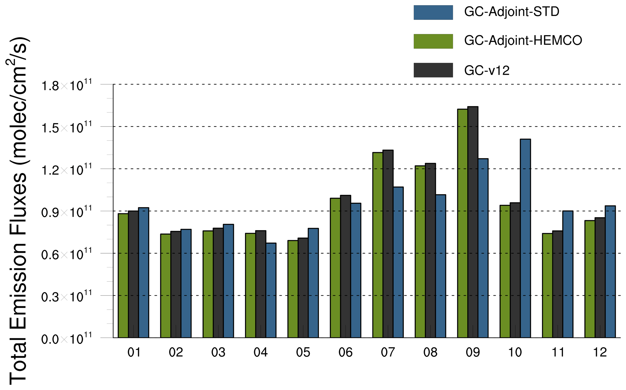
Figure 3 Monthly variation in combustion CO emissions in 2015 from GC-v12, GC-Adjoint-HEMCO and GC-Adjoint-STD.

2.4 Updates in CO chemical sources and sinks

The biogenic emissions in GC-Adjoint-STD are from the Model of Emissions of Gases and Aerosols from Nature, version 2.0 (MEGANv2.0, Guenther et al., 2006) in the full chemistry simulation but are from GEIA in the tagged-CO simulation (Fig. S7). Fisher et al. (2017) demonstrated improvement in modeled CO concentrations in the tagged-CO simulation by reading archived VOC- and CH₄-generated CO fields provided by the full chemistry simulation. The archived VOC- and CH₄-generated CO fields in 2013 (PCO_3Dglobal.geosfp.4x5.nc) were set as the default CO chemical sources in the tagged-CO simulation in GC-v12 and were supported in GC-Adjoint-HEMCO. As shown in Table 2, the CO chemical sources (columns) obtained by reading the archived VOC- and CH₄-generated CO fields demonstrate good agreement between GC-v12 and GC-Adjoint-HEMCO. However, they are 30 %–60 % lower than those in GEIA in GC-Adjoint-STD, and this difference could be partially associated with the inconsistency between the archived VOC-generated CO fields in 2013 and the actual meteorological data in 2015 in the simulation.

The default CH₄-generated CO emissions in GC-Adjoint-STD (Fig. S8) are calculated based on averaged CH₄ concentrations in four latitudinal bands (90–30^∘ S, 30–00^∘ S, 00–30^∘ N, 30–90^∘ N), which are based on Climate Monitoring and Diagnostics Laboratory (CMDL) surface observations and Intergovernmental Panel on Climate Change (IPCC) future scenarios. As shown in Table 2, there are good agreements in the CH₄-generated CO emissions between GC-v12 and GC-Adjoint-HEMCO when reading PCO_3Dglobal.geosfp.4x5.nc, and they are 20 %–60 % lower than those in CMDL/IPCC in GC-Adjoint-STD. Furthermore, the default archived monthly OH fields were updated following GC-v12 with updated calculations for the decay rate (KRATE, from JPL 03 to JPL 2006) in GC-Adjoint-HEMCO. The subsequent CO sinks (Fig. S9) in GC-v12 and GC-Adjoint-HEMCO are 20 %–40 % higher than those in GC-Adjoint-STD.

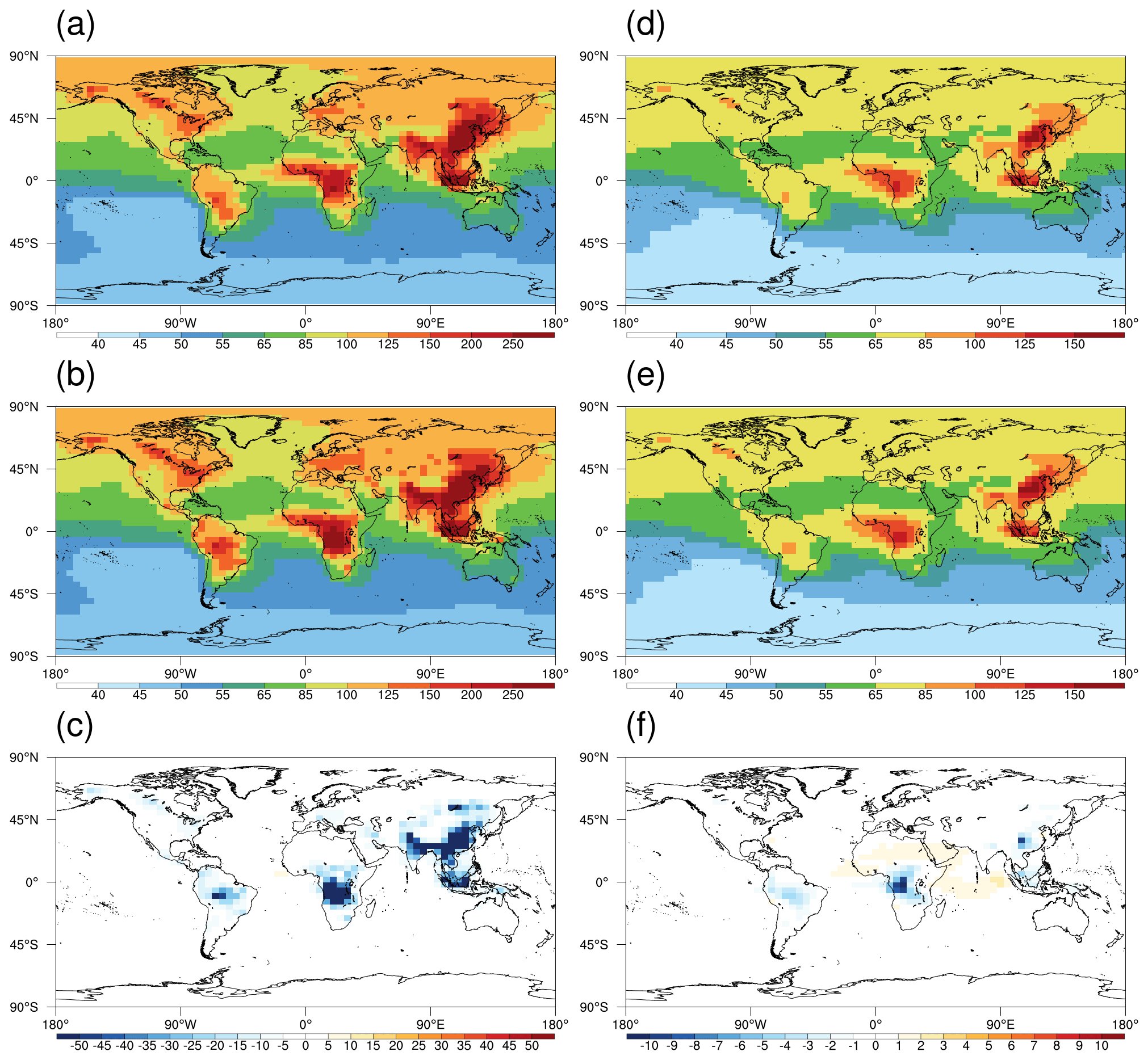
Figure 4 Averages of surface CO concentrations (unit: ppbv) in 2015 from (a) GC-Adjoint-HEMCO driven by MERRA-2, (b) GC-Adjoint-HEMCO driven by GEOS-FP and (c) their difference; (d–f) same as panels (a–c) but for CO columns (column-averaged dry-air mole fractions, Xco).

2.5 Updates in meteorological data

The MERRA-2 meteorological data (1979–present) are supported in GC-Adjoint-HEMCO to ensure long-term consistency in the meteorological data in the analyses. The code porting to support MERRA-2 follows the current framework of the adjoint of the GEOS-Chem model, particularly because the meteorological variables and vertical resolutions of MERRA-2 are the same as those of GEOS-FP (2012–present), while GEOS-FP is already supported by GC-Adjoint-STD. Figure 4a–b show the averages of surface CO concentrations in 2015 from GC-Adjoint-HEMCO driven by MERRA-2 and GEOS-FP, respectively. Our results demonstrate lower surface CO concentrations driven by MERRA-2 (Fig. 4c), although there is good agreement in the spatial distributions of CO concentrations. Similarly, Fig. 4d–f show the averages of CO columns in 2015 from GC-Adjoint-HEMCO driven by MERRA-2 and GEOS-FP and their differences. Despite the noticeable differences in surface CO concentrations (Fig. 4c), the differences in CO columns (Fig. 4f) are much smaller, and the modeled CO columns driven by MERRA-2 are higher than those driven by GEOS-FP over the Indian Ocean. The discrepancy between surface and column CO in Fig. 4 may reflect the impacts of different convective transports on the modeled CO concentrations.

2.6 MOPITT CO measurements

The MOPITT data used here were obtained from the joint retrieval (V7J) of CO from thermal infrared (TIR, 4.7 µm) and near-infrared (NIR, 2.3 µm) radiances using an optimal estimation approach (Worden et al., 2010; Deeter et al., 2017). The retrieved volume mixing ratios (VMRs) are reported as layer averages of 10 pressure levels with a footprint of 22 km ×22 km. Following Jiang et al. (2017), we reject MOPITT data with CO column amounts less than 5×10¹⁷ molec. cm⁻² and with low cloud observations. Since the NIR channel measures reflected solar radiation, only daytime data are considered.

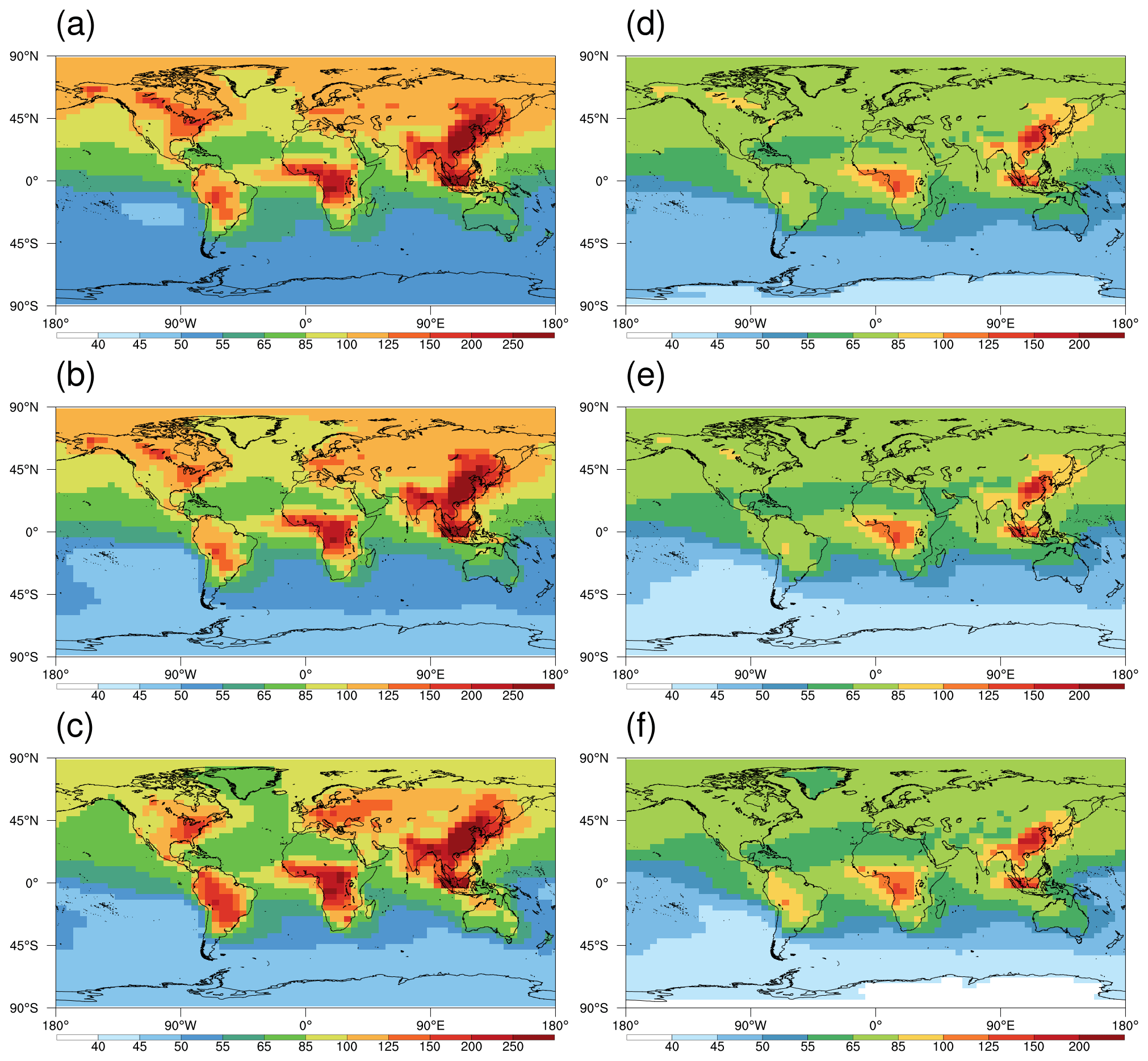
Figure 5 Averages of surface CO concentrations (unit: ppbv) in 2015 from (a) GC-v12, (b) GC-Adjoint-HEMCO and (c) GC-Adjoint-STD; (d–f) same as panels (a–c) but for CO columns (column-averaged dry-air mole fractions, Xco).

3 Model evaluation and application

3.1 Model performances in forward and backward simulations

The reasonable emissions in the diagnostic outputs in Sect. 2 do not necessarily mean the correct integration of emissions in the assimilations. Consequently, here, we evaluate the performance of GC-Adjoint-HEMCO in forward simulations. Figure 5 shows the averages of surface and column CO concentrations in 2015 from GC-v12, GC-Adjoint-HEMCO and GC-Adjoint-STD. As shown in Table 2, the regional differences between GC-v12 and GC-Adjoint-HEMCO are 2.6 %, −5.7 %, −4.6 %, −1.7 %, −1.4 % and −3.6 % in surface CO concentrations and −2.3 %, −3.6 %, −3.3 %, −3.1 %, −3.3 % and −4.1 % in CO columns over Asia, North America, Africa, South America, Europe and Australia, respectively. There are larger regional differences in CO concentrations between GC-v12 and GC-Adjoint-STD: 4.6 %, −10.1 %, 6.3 %, 22.5 %, 6.4 % and 25.7 % in surface CO concentrations and −0.7 %, −9.9 %, 2.5 %, 8.0 %, −5.8 % and 8.5 % in CO columns over Asia, North America, Africa, South America, Europe and Australia, respectively. The agreement between GC-v12 and GC-Adjoint-HEMCO confirms the reliability of GC-Adjoint-HEMCO in forward simulations, while the small differences in CO concentrations between GC-v12 and GC-Adjoint-HEMCO are expected in view of the comparable differences in regional emissions, chemical sources and sinks, as shown in Table 2.

In addition to forward simulations, the reliability of 4D-Var assimilation also relies on the accuracy of the adjoint-based sensitivities, which are obtained by the backward simulations of adjoint tracers and the combination of adjoint tracers with emissions. As mentioned in Sect. 2.2, we have made corresponding modifications to both forward and backward modules. Consequently, here, we further evaluate the performance of GC-Adjoint-HEMCO in backward simulations. Here, the adjoint gradients are simplified as follows:

$$\begin{array}{}\text{(3)}& {\mathrm{\nabla }}_{\mathit{x}}J\left(\mathit{x}\right)={\displaystyle \frac{\partial {\mathbf{F}}_N}{\partial \mathit{x}}}.\end{array}$$

The adjoint gradients (Eq. 3) represent the sensitivities of modeled atmospheric compositions at the final time step (i.e., i=N) to emissions, which were then compared with the finite-difference gradients calculated with

$$\begin{array}{}\text{(4)}& \mathrm{\Lambda }={\displaystyle \frac{J\left(\mathit{x}+\mathit{\delta }\mathit{x}\right)-J\left(\mathit{x}-\mathit{\delta }\mathit{x}\right)}{\mathrm{2}\mathit{\delta }\mathit{x}}}.\end{array}$$

Here, the finite-difference gradients represent the response of modeled atmospheric compositions at the final time step to finite perturbations in emissions provided by the forward simulations (δx=10 % in this work).

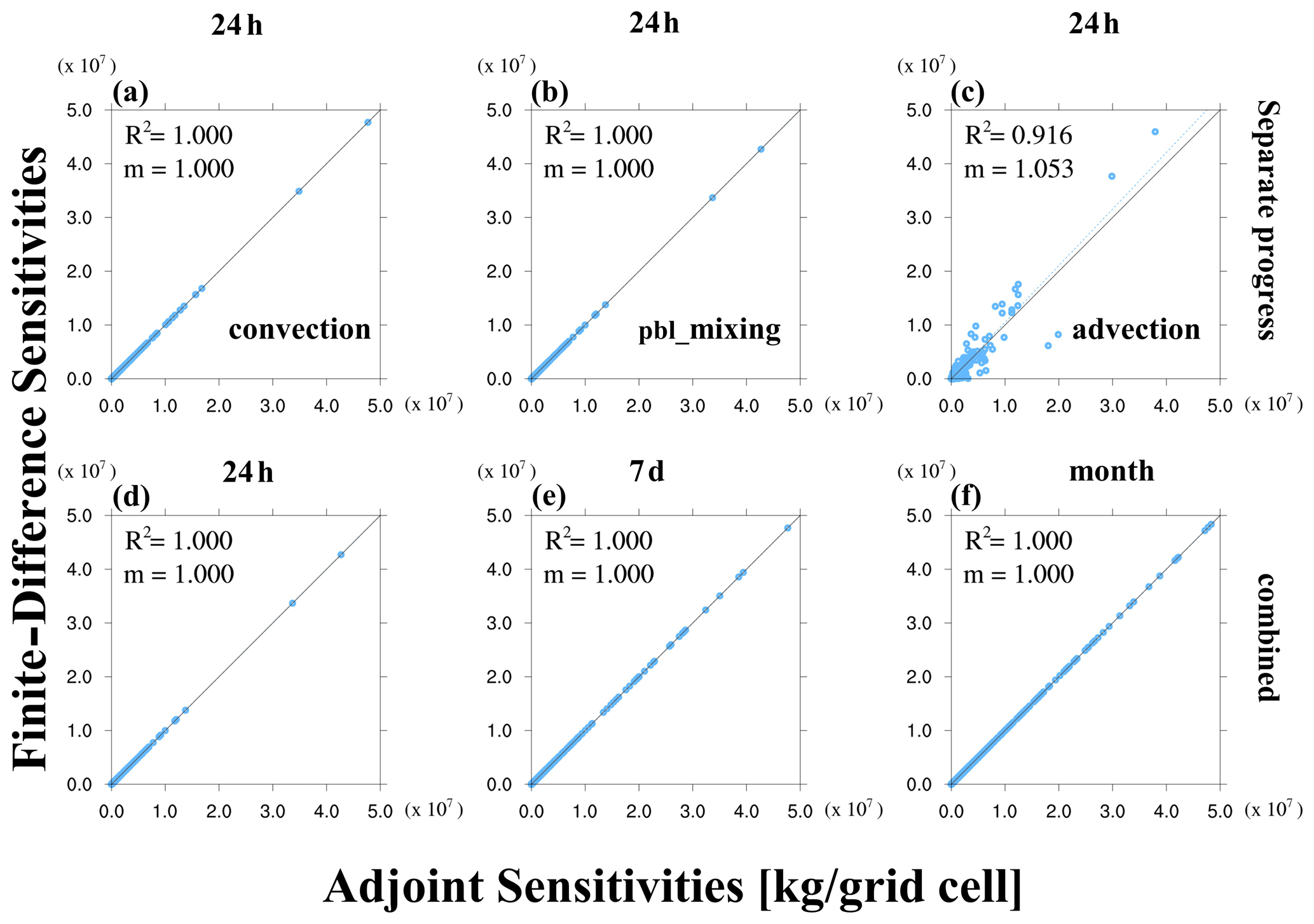
Figure 6 Comparison of sensitivities of global CO concentrations (LFD_GLOB and model level 1) to CO emission scaling factors calculated using the adjoint method vs. the finite-difference method. (a–c) The effects of convection, PBL mixing and advection with 24 h assimilation window. (d–f) The combined effects (the advection process is turned off) with increased assimilation windows.

Figure 6a–c show the comparison of adjoint and finite-difference gradients of global surface CO concentrations to CO emissions with a 24 h assimilation window by turning on the convection, planetary boundary layer mixing and advection processes individually. We find good consistency in the gradients with respect to convection and planetary boundary layer (PBL) mixing. The larger deviation with respect to advection is caused by the discrete advection algorithm in forward simulations and the continuous advection algorithm in backward simulations (Henze et al., 2007). Figure 6d–f further exhibit the effects of combined model processes (turning off advection as suggested by Henze et al., 2007). We find good agreement between the adjoint and finite-difference gradients with different assimilation windows (24 h, 7 d and 1 month). Moreover, Figs. S10 and S11 demonstrate the comparisons of sensitivities at higher model levels within the PBL and free troposphere by showing consistent results in relation to Fig. 6. This confirms the consistency in the impacts of emissions on modeled atmospheric compositions between the forward and backward simulations, which is the prerequisite for more detailed evaluations in the following sections.

3.2 Observing system simulation experiments with pseudo-CO observations

Here, we further evaluate the performance of GC-Adjoint-HEMCO in 4D-Var assimilations. OSSE is a useful method and has been widely used to evaluate the performance of various data assimilation systems (Jones et al., 2003; Barré et al., 2015; Shu et al., 2022). In contrast to assimilations by assimilating actual atmospheric observations, pseudo-observations are usually generated by model simulations and then assimilated in OSSE. The true atmospheric states are known in OSSEs as they are used to produce the pseudo-observations, and consequently, the difference between assimilated and true atmospheric states describes the capability of the assimilation systems to converge to the true atmospheric states in assimilations when assimilating actual observations.

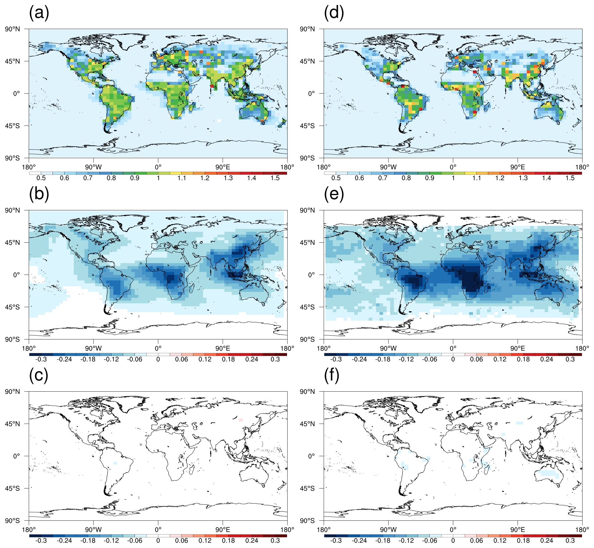
Figure 7 (a) Annual scaling factors in OSSE-FullOBS. The scaling factors represent the ratio of the estimated to true emissions. The ratio for the first guess is 0.5. The actual value is 1.0. (b–c) The a priori and a posteriori biases calculated by (model–observation)/observation in OSSE-Full. (d–f) Same as panels (a–c) but for OSSE-MOPITT.

The pseudo-observations in this work are produced by archiving CO concentrations from GC-Adjoint-HEMCO forward simulations with the CO emissions unchanged (i.e., the default CO emission inventory such as CEDS, MIX and NEI2011). According to the usage of pseudo-observations, two types of OSSEs are performed in this work: (1) full modeled CO fields are assimilated as pseudo-observations so that we have pseudo-CO observations at every grid, level and time step (hereafter referred to as OSSE-FullOBS). This experiment is designed to evaluate the performance of the assimilation system under ideal conditions with full coverage of observations. (2) The modeled CO fields are sampled at the locations and times of MOPITT CO observations and smoothed with MOPITT a priori concentrations and averaging kernels to produce MOPITT-like pseudo-CO observations (hereafter referred to as OSSE-MOPITT). This experiment is designed to evaluate the performance of the assimilation system under actual conditions with limited coverage of observations.

In the inverse analysis with the pseudo-CO observations, we reduce the anthropogenic CO emissions by 50 % so that the objective of the OSSE is to produce scaling factors that can return the source estimate to the default emissions (i.e., scaling factors of 1.0). Figure 7a shows the annual scaling factors in 2015 in OSSE-FullOBS. After 40 iterations, the a posteriori anthropogenic CO emission estimates converge to the true states in all major emission regions. As shown in Table 3, the regional scaling factors of OSSE-FullOBS are 1.00, 0.97, 0.97, 1.00, 0.98 and 0.94 for anthropogenic CO emissions over Asia, North America, Africa, South America, Europe and Australia, respectively.

Table 3 Annual scaling factors of anthropogenic CO emissions in OSSEs. The scaling factors represent the ratio of the estimated to true emissions. The ratio for the first guess is 0.5. The actual value is 1.0. The pseudo-observations are produced by the GC-Adjoint-HEMCO forward simulation. The full modeled CO fields are used in OSSE-FullOBS as pseudo-CO observations. The modeled CO fields are smoothed with MOPITT averaging kernels to produce MOPITT-like pseudo-CO observations in OSSE-MOPITT.

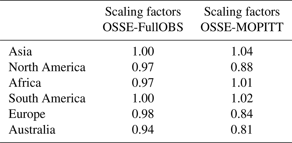
Furthermore, Fig. 7d shows the annual scaling factors in OSSE-MOPITT, which are noticeably worse than those in Fig. 7a. The regional scaling factors of OSSE-MOPITT are 1.04, 0.88, 1.01, 1.02, 0.84 and 0.81 for anthropogenic CO emissions over Asia, North America, Africa, South America, Europe and Australia, respectively. With respect to OSSE-FullOBS, the limited coverage of observations in OSSE-MOPITT has resulted in approximately 15 % underestimations in the a posteriori CO emission estimates over North America and Europe. In addition, Fig. 7b–c and e–f show the a priori and a posteriori biases in the modeled CO columns. We find dramatic improvements in the modeled CO columns, which confirms the reliability of the 4D-Var assimilation system. The difference between Figs. 7b and 6e reflects the influence of the application of MOPITT averaging kernels, which lead to larger negative biases in the a priori simulation. It should be noted that we cannot expect comparable improvement in the actual assimilations because of the potential effects of model and observation errors.

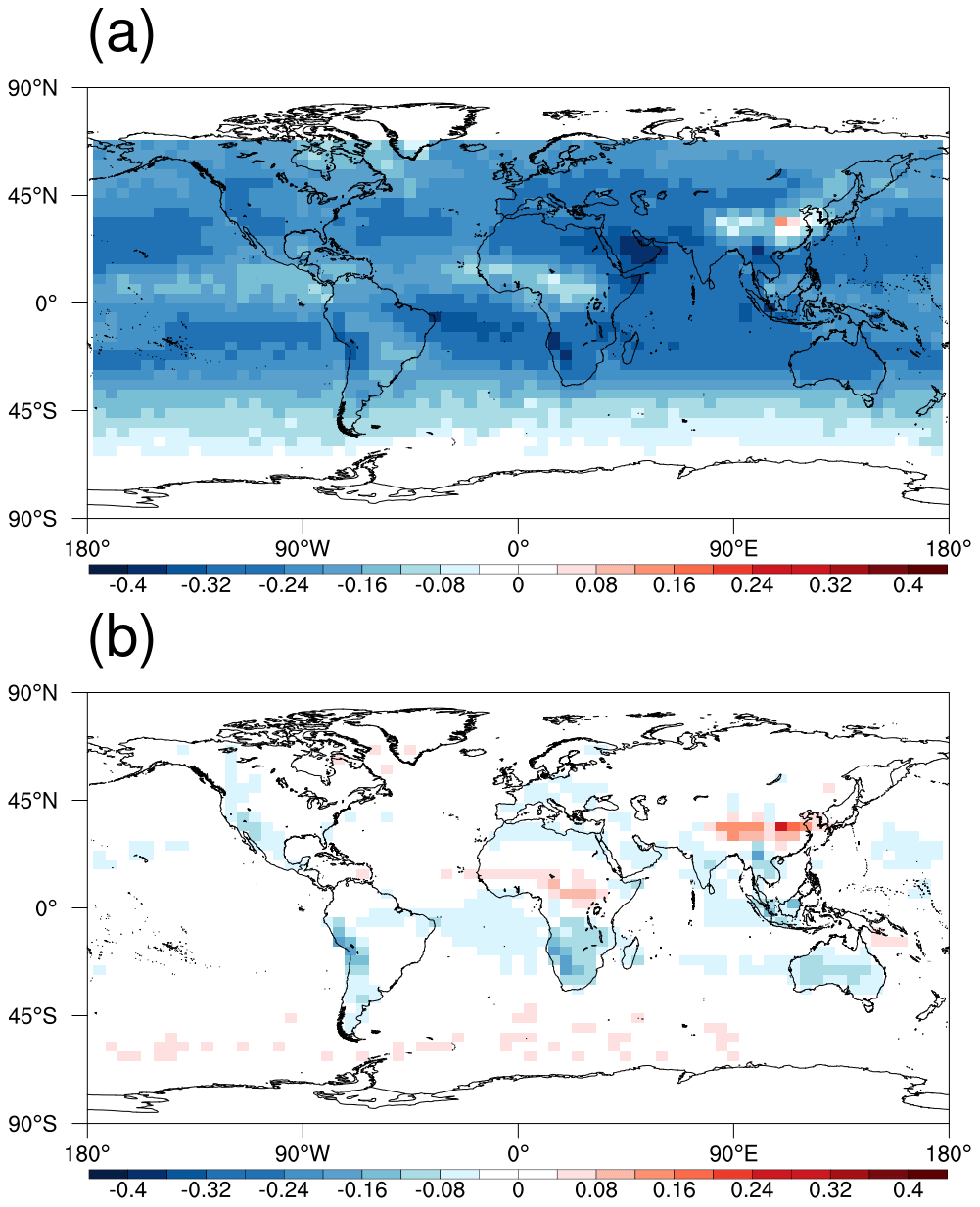
Figure 8 (a) Biases in monthly initial CO conditions in 2015 in the original GEOS-Chem simulation. (b) Same as panel (a) but with optimized initial CO conditions provided by sub-optimal sequential Kalman filter. The biases are calculated by (model–MOPITT)/MOPITT.

3.3 Anthropogenic CO emissions constrained with MOPITT CO observations

As an example of the application of GC-Adjoint-HEMCO, here, we constrain anthropogenic CO emissions in 2015 by assimilating MOPITT CO observations. Figure 8a shows the relative differences between modeled and MOPITT CO columns at the beginning of each month in 2015 (i.e., biases in monthly initial CO conditions) in the original GEOS-Chem simulations. We find dramatic underestimations in the modeled CO columns of approximately 30 %–40 %. As indicated by previous studies (Jiang et al., 2013, 2017), the biases in monthly initial CO conditions are caused by model biases in CO concentrations accumulated in previous months. Considering that the lifetime of CO is approximately 2–3 months, the negative biases in the initial conditions can result in negative biases in the modeled CO concentration in the following month. A lack of consideration of these biases, as shown in Fig. 8a, can thus result in overestimations in the derived monthly CO emission estimates because the assimilation system will tend to adjust emissions to reduce the initial condition-induced biases.

Table 4 Regional anthropogenic CO emissions (in Tg yr⁻¹) and annual scaling factors in 2015 in this work and Jiang et al. (2017).

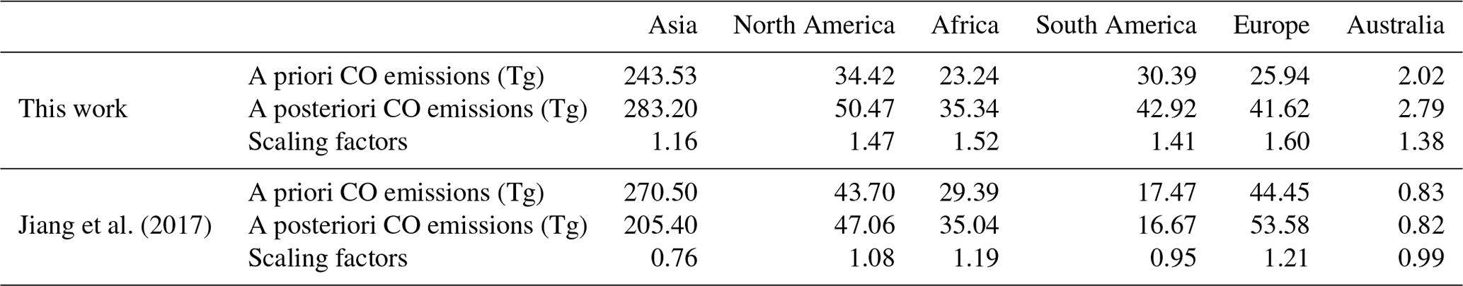
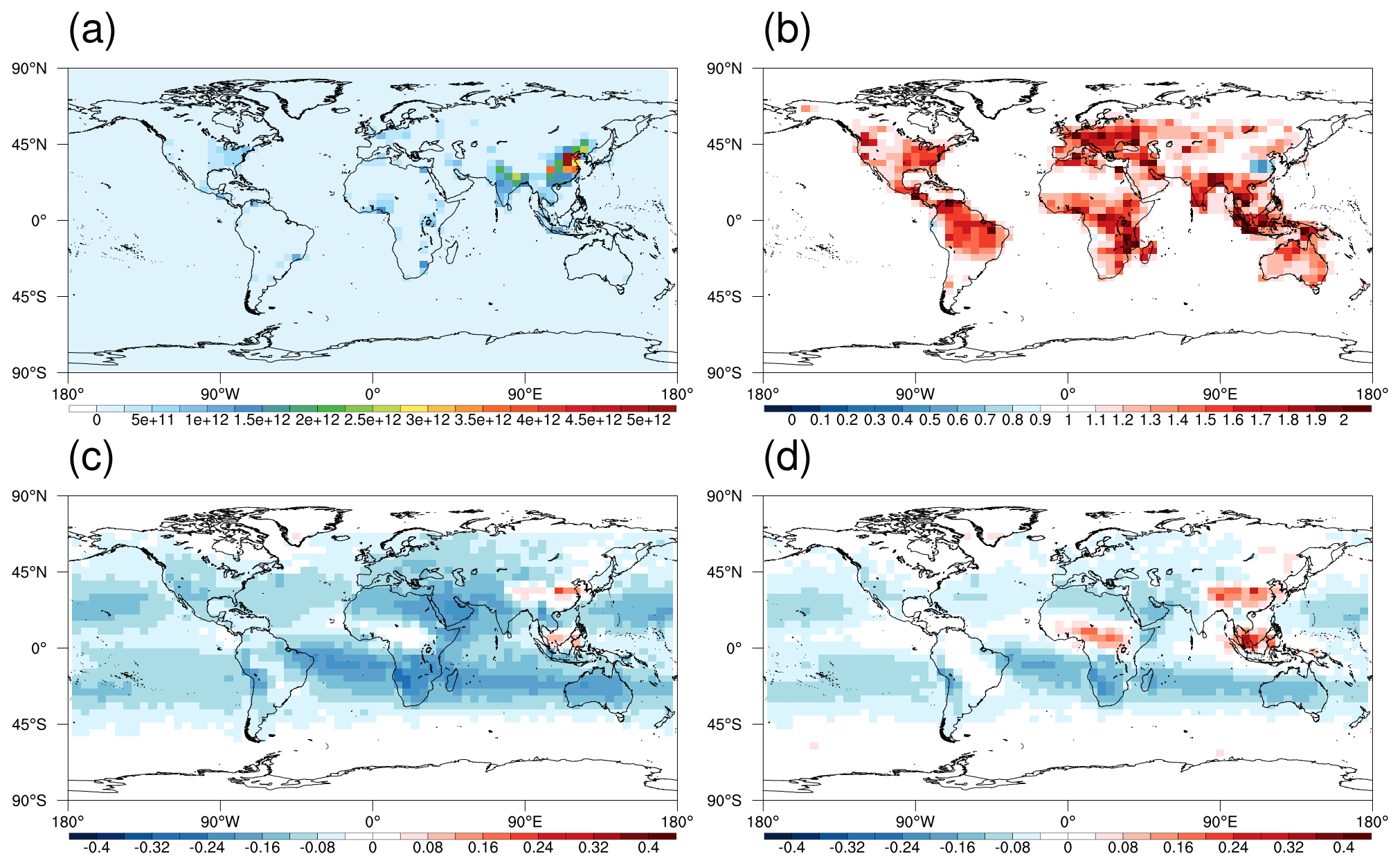
Figure 9 (a) A priori anthropogenic CO emissions in 2015 (in molec. cm² s⁻¹). (b) Annual scaling factors for CO emissions in 2015. The scaling factors represent the ratio of the estimated to true emissions. (c–d) The a priori and a posteriori biases calculated by (model–MOPITT)/MOPITT.

Following Jiang et al. (2017), a sub-optimal sequential Kalman filter (Todling and Cohn, 1994; Tang et al., 2022) was employed in this work to optimize the modeled CO concentrations with an hourly resolution by combining GC-Adjoint-HEMCO forward simulations and MOPITT CO observations. The CO concentrations provided by the Kalman filter assimilations were archived at the beginning of each month and were used as the optimized monthly initial CO conditions in the inverse analysis. As shown in Fig. 8b, the biases in the modeled CO columns in the optimized initial CO conditions are pronouncedly lower than those in the original simulation (Fig. 8a). The optimization of the initial CO conditions is essential for our inverse analysis as it can ensure that the adjustments in CO emissions are dominated by the differences between simulations and observations in the current month instead of the 30 %–40 % underestimations in CO columns accumulated in previous months.

Figure 9a shows the distribution of a priori anthropogenic CO emissions in 2015. The regional a priori anthropogenic CO emissions (as shown in Table 4) are 243.53, 34.42, 23.24, 30.39, 25.94 and 2.02 Tg yr⁻¹ over Asia, North America, Africa, South America, Europe and Australia, respectively. As shown in Fig. 9b, our inverse analysis suggests a wide distribution of underestimations in the a priori anthropogenic CO emissions in 2015 except in China. The regional scaling factors (Table 4) are 1.16, 1.47, 1.52, 1.41, 1.60 and 1.38, and the a posteriori anthropogenic CO emissions are 283.20, 50.47, 35.34, 42.92, 41.62 and 2.79 Tg yr⁻¹ over Asia, North America, Africa, South America, Europe and Australia, respectively. As shown in Fig. 9c, we find noticeable underestimations in the modeled CO columns in the a priori simulations despite the negative biases being much weaker than those in Fig. 8a due to the optimization of the initial CO conditions. The negative biases are effectively reduced in the a posteriori simulation driven by the a posteriori CO emission estimates (Fig. 9d).

Finally, we compare the a posteriori CO emission estimates in this work with those of Jiang et al. (2017), who constrained CO emissions in 2001–2015 with GC-Adjoint-STD by assimilating the same MOPITT CO observations. As shown in Table 4, the a posteriori anthropogenic CO emission estimates in this work match well with those of Jiang et al. (2017) in North America and Africa but are 38 %, 157 % and 228 % higher than those in Jiang et al. (2017) in Asia, South America and Australia, respectively. A major discrepancy between this work and Jiang et al. (2017) is the treatment of ocean grids. Jiang et al. (2017) defined ocean grids as continental boundary conditions, which were rewritten hourly using the optimized CO concentrations archived from the sub-optimal sequential Kalman filter by assimilating MOPITT CO observations. Only MOPITT data over land were assimilated in the 4D-Var assimilations in Jiang et al. (2017) without any change in CO distribution over the ocean. In addition, the large differences in chemical sources and sinks between GC-Adjoint-HEMCO and GC-Adjoint-STD – for example, 40 %–60 % lower VOC-generated CO emissions and 20 %–40 % higher CO sinks in GC-Adjoint-HEMCO, as shown in Table 2 – may also contribute to the discrepancy in the derived a posteriori CO emission estimates.

As shown in Fig. 9d, the a posteriori simulation demonstrates positive biases in CO columns over China and southeast Asia, which is a signal of overestimated local CO emissions; meanwhile, the negative biases over the northern Pacific Ocean are reduced in the a posteriori simulation. The negative biases over the remote ocean are more affected by CO chemical sources and sinks; however, biases in chemical sources cannot be effectively adjusted because of the global uniform scaling factor for CH₄-generated CO emissions; biases in chemical sinks cannot be adjusted because of the fixed OH fields in the tagged-CO simulation. Jiang et al. (2017) tried to address this problem by defining continental boundary conditions so that the inverse analysis is dominated by local MOPITT observations to avoid the influence of model biases accumulated within the long-range transport. Conversely, CO emissions over China and southeast Asia are overestimated in this work to offset the negative biases over the northern Pacific Ocean. We expect similar overestimations in the a posteriori CO emission estimates over South America, southern Africa and Australia in this work because it is the effective pathway to reduce the negative bias over the ocean in the Southern Hemisphere.

4 Conclusions

This work demonstrates our efforts in the development of a new framework to facilitate emission inventory updates in the adjoint of the GEOS-Chem model. The major advantage of this new framework is good readability and extensibility, which allows us to conveniently support HEMCO emission inventories, including CEDS, MIX, NEI2011, DICE_AF, AF_EDGAR43, APEI and GFED4. The updated emission inventories are critical for reliable sensitivity analyses, as well as better convergence of assimilations by setting a more reasonable a priori penalty in the cost function. Second, we developed new modules to support MERRA-2 meteorological data, which allows us to perform long-term inverse analyses with consistent meteorological data for the period 1979–present. We evaluated the performances of the developed capabilities by validating the diagnostic outputs of CO emissions, modeled surface and column CO concentrations in forward simulations, and adjoint gradients of global CO concentrations to CO emissions with respect to the finite-difference gradients.

Two types of OSSEs were conducted to evaluate the model performance in 4D-Var assimilations. The a posteriori CO emissions converged to the true states in all major emission regions with fully covered pseudo-CO observations; the limited coverage of observations from sampling the pseudo-CO observations at the locations and times of MOPITT CO observations and smoothing with MOPITT averaging kernels resulted in underestimations of approximately 15 % in the a posteriori CO emissions over North America and Europe. Furthermore, as an example application of the developed capabilities, we constrain anthropogenic CO emissions in 2015 by assimilating MOPITT CO observations. The a posteriori anthropogenic CO emission estimates derived in this work match well with those of Jiang et al. (2017) in North America and Africa but are overestimated in Asia, South America and Australia, which could be associated with the different treatment of MOPITT CO observations over ocean grids and the large differences in CO chemical sources and sinks. The capabilities developed in this work are a useful extension for the adjoint of the GEOS-Chem model. More efforts are needed to support emissions inventories associated with full chemistry simulations, as well as for integration of these capabilities with the standard GEOS-Chem adjoint code base for better development of the community of the adjoint of the GEOS-Chem model.