A robust error correction method for numerical weather prediction wind speed based on Bayesian optimization, variational mode decomposition, principal component analysis, and random forest: VMD-PCA-RF (version 1.0.0)

Accurate wind speed prediction is crucial for the safe and efficient utilization of wind resources. However, current single-value deterministic numerical weather prediction methods employed by wind farms do not adequately meet the actual needs of power grid dispatching. In this study, we propose a new hybrid forecasting method for correcting 10 m wind speed predictions made by the Weather Research and Forecasting (WRF) model. Our approach incorporates variational mode decomposition (VMD), principal component analysis (PCA), and five artificial intelligence algorithms: deep belief network (DBN), multilayer perceptron (MLP), random forest (RF), eXtreme gradient boosting (XGBoost), light gradient boosting machine (lightGBM), and the Bayesian optimization algorithm (BOA). We first predict wind speeds using the WRF model, with initial and lateral boundary conditions from the Global Forecast System (GFS). We then perform two sets of experiments with different input factors and apply BOA optimization to tune the four artificial intelligence models, ultimately building the final models. Furthermore, we compare the aforementioned five optimal artificial intelligence models suitable for five provinces in southern China in the wintertime: VMD-PCA-RF in December 2021 and VMD-PCA-lightGBM in January 2022. We find that the VMD-PCA-RF evaluation indices exhibit relative stability over nearly a year: the correlation coefficient (R) is above 0.6, forecasting accuracy (FA) is above 85 %, mean absolute error (MAE) is below 0.6 m s⁻¹, root mean square error (RMSE) is below 0.8 m s⁻¹, relative mean absolute error (rMAE) is below 60 %, and relative root mean square error (rRMSE) is below 75 %. Thus, for its promising performance and excellent year-round robustness, we recommend adopting the proposed VMD-PCA-RF method for improved wind speed prediction in models.

1 Introduction

Sustainable energy plays a vital role in reducing carbon footprint and increasing system reliability (Hanifi et al., 2020). As renewable energy sources have a negligible carbon footprint, they have become the preferred choice for many industries in the power sector (Dhiman and Deb, 2020). Among these sources, wind energy is a crucial low-carbon energy technology with the potential to become a sustainable energy source (Tascikaraoglu and Uzunoglu, 2014). In 2022, the global wind power capacity reached 906 GW, with a 9 % year-on-year increase due to a newly installed capacity of 77.6 GW. The global onshore wind market increased by 68.8 GW, while facing a 5 % growth decline compared to the previous year. Such change is attributed to a slowdown in China and the US, the world's two largest wind markets that account for over two-thirds of the world's onshore wind farm installations (Joyce and Feng, 2023). The instability and unpredictability of wind power generation can lead to instability in the power system. In addition, the decline of the wind energy market also makes it more challenging to improve the accuracy of wind speed forecasts. An accurate wind speed prediction method is needed to reduce the instability risk of the power system and the economic loss of wind power enterprises (Huang et al., 2019). Therefore, accurate and stable wind speed prediction (WSP) is very important for the safe and stable operation of the power grid system and for improving the utilization rate of wind energy and economic development (Guo et al., 2021; Xiong et al., 2022; Tang et al., 2021).

Current WSP algorithms are primarily categorized into physical algorithms (Zhao et al., 2016), statistical algorithms (Wang and Hu, 2015; Barthelmie et al., 1993), machine learning (ML) algorithms (Huang et al., 2019; Salcedo-Sanz et al., 2011; Ma et al., 2020), and hybrid algorithms (Deng et al., 2020; Xu et al., 2021; Zhao et al., 2019; Xiong et al., 2022; Tang et al., 2021). Physical methods, such as numerical weather prediction (NWP), are commonly used in wind speed forecasting. NWP, which accounts for atmospheric processes and physical laws, solves discrete mass, momentum, and energy conservation equations along with other fundamental physical principles, establishing itself as a widely adopted and reliable physical method. Currently, the High-resolution Limited Area Model (HIRLAM) (Služenikina and Männik, 2016), the European Centre for Medium-Range Weather Forecasts (ECMWF) model, the Fifth-Generation Mesoscale Model (MM5) (Salcedo-Sanz et al., 2009), and the Weather Research and Forecasting (WRF) model (Skamarock et al., 2021) are extensively utilized for wind speed prediction. However, NWP modeling faces challenges due to the selection of parameterization schemes, such as model microphysics and systematic errors, which exhibit temporal and spatial differences and uncertainties. These uncertainties hinder the accuracy of NWP models in wind speed prediction, making it difficult to meet the rising demands of the grid system (Zhao et al., 2019; Xu et al., 2021).

Studies have demonstrated that enhancing the accuracy of numerical weather prediction (NWP) models and correcting prediction errors can effectively minimize the errors associated with wind speed prediction. These research endeavors have typically sought to optimize the physical and dynamic parameters of the NWP model (Cheng et al., 2013), refine the model structure (Jiménez and Dudhia, 2012), or improve the accuracy of model inputs through preprocessing and denoising techniques (Xu et al., 2015). Additionally, improving initial field error through methods, such as target observation and data assimilation (Williams et al., 2013), can also minimize wind speed errors predicted by NWP models.

Physical methods are generally more appropriate for long-term wind speed prediction, such as those 48–72 h in advance, while their practical application in short-term forecasting is limited (Zhao et al., 2019; Deng et al., 2020; James et al., 2018). In contrast, statistical methods utilize historical data to establish a relationship between input and output variables and are therefore well suited for short-term wind speed prediction. They are usually time series models, such as autoregressive moving average (ARMA) (Erdem and Shi, 2011) and autoregressive integrated moving average (ARIMA) (Wang and Hu, 2015), whereas filtering models (Cassola and Burlando, 2012; Chen and Yu, 2014), machine learning models (Hu et al., 2013), and hybrid models (Huang et al., 2019) have been gradually developed to further improve wind speed prediction accuracy.

With purely statistical models becoming less suitable for wind speed predictions beyond 6 h, the use of a combination of physical and statistical methods has gained growing interest (Zjavka, 2015; Xu et al., 2021). The error correction model improves the accuracy of the NWP model by training on the relationship between the NWP predictor variables and the observed correlation variables (Sun et al., 2019). However, traditional error prediction models rely solely on historical wind speed sequences as input factors (Deng et al., 2020; Guo et al., 2021) and do not incorporate the characteristic meteorological factors forecasted by the WRF model. Studies have shown that considering all relevant historical meteorological factors can lead to more accurate predictions compared to only taking into account historical wind speed (Z. Zhang et al., 2019). Therefore, it is crucial to include meteorological characteristic factors as input in the prediction model.

For an error prediction model, wind speed is the most important input factor. Traditionally, the error prediction model uses historical wind speed data as input, without any feature selection. Feature selection methods, such as filtering methods, are commonly used in time series analysis. Currently, empirical mode decomposition (EMD) (Liu et al., 2018; Guo et al., 2012), ensemble empirical mode decomposition (EEMD) (Wang et al., 2017), wavelet decomposition (WD) (Y. Zhang et al., 2019), variational mode decomposition (VMD) (Hu et al., 2021; D. Zhang et al., 2019), and other filtering methods are used to select key features in the wind speed data. As mentioned above, studies have shown that these feature selection methods can effectively extract the hidden features in the wind speed series to improve wind speed prediction accuracy. However, despite the effectiveness of wind speed filtering methods in wind speed prediction, only a few studies have applied these methods to the correction of wind speed errors in NWP forecasting (Xu et al., 2021; Li et al., 2022).

In addition, traditional error correction methods generally adopt linear regression (Dong et al., 2013), multiple linear regression (Liu et al., 2016), machine learning (Salcedo-Sanz et al., 2011), and deep learning algorithms (Z. Zhang et al., 2019). However, the efficacy of machine learning and deep learning algorithms is highly dependent on the selection of model parameters (Guo et al., 2021; Xiong et al., 2022). The Bayesian optimization algorithm (Li and Shi, 2010; Guo et al., 2021) is considered a relatively advanced algorithm for optimizing model parameters and has been widely used in MATLAB and Python packages.

In this study, we investigate a multi-step wind speed forecasting model that combines NWP simulation and an error correction strategy. We present two sets of experiments divided into three steps. (1) We use the first group of experiments to extract hidden features from various meteorological elements forecasted by NWP; the second group of experiments mainly focuses on the wind speed forecast of NWP, and the VMD-PCA algorithm is used to extract the hidden features in the forecasted wind speed. Each set of experimental input factors is matched with the actual 10 m wind speed data of 410 stations in time and space. (2) We employ four advanced machine learning algorithms optimized by the BOA algorithm and DBN deep learning algorithm to train the two groups of experiments and perform 5-fold cross-validation. (3) We analyze six distinct wind speed error indicators to compare and identify the most suitable wind speed error correction schemes for the five southern provinces (Yunnan, Guizhou, Guangxi, Guangdong, Hainan) in winter and throughout most of the year. The remainder of this paper is organized into sections discussing the effects of the BOA-VMD-PCA approach, the interpretability of RF feature importance, and the stability analysis of the proposed models.

2 Data and methods

2.1 Data

The observed data come from the China Meteorological Administration Land Data Assimilation System (CLDAS-V2.0) real-time product dataset. According to the description of the documents on the official website (https://data.cma.cn/data/cdcdetail/dataCode/NAFP_CLDAS2.0_RT.html, last access: 13 October 2023), the dataset is constructed through the integration of multiple sources, including ground and satellite data, and is refined using advanced techniques such as multi-grid variational assimilation, physical inversion, and terrain correction. This dataset exhibits superior quality in comparison to other products, offering higher spatial and temporal resolutions. The target observation data include 2 m air temperature, 2 m specific humidity, 10 m wind speed, surface pressure, and precipitation. These data are processed by the China Meteorological Public Service Center to an equivalent latitude and longitude grid scale, covering a geographical range of 15–32.97^∘ N and 94–120.97^∘ E. The spatial resolution of the grid is 0.03^∘ × 0.03^∘ (3 km by 3 km), and the temporal resolution is 1 h. The China Meteorological Public Service Center applied the nearest neighbor interpolation for precipitation and bilinear interpolation for the other four meteorological elements with downscaling from 3 km to 410 sites. We select the 10 m wind speed data of 410 sites, as illustrated in Fig. 1.

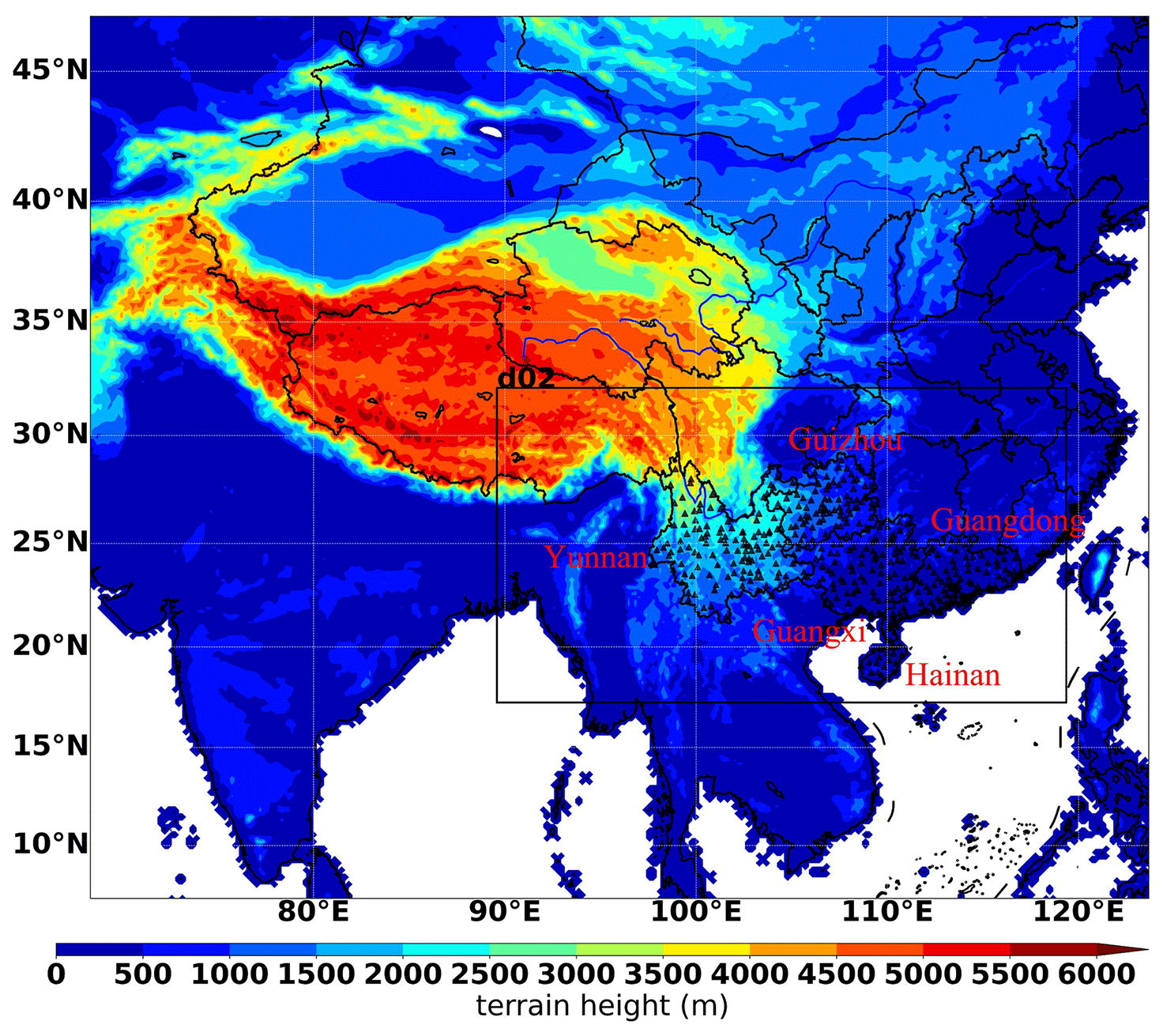
Figure 1 WRF model simulation area elevation diagram (d02 represents the nested area of the second layer of the WRF model, and the black triangles represent the meteorological sites).

2.2 Methods

2.2.1 WRF simulation

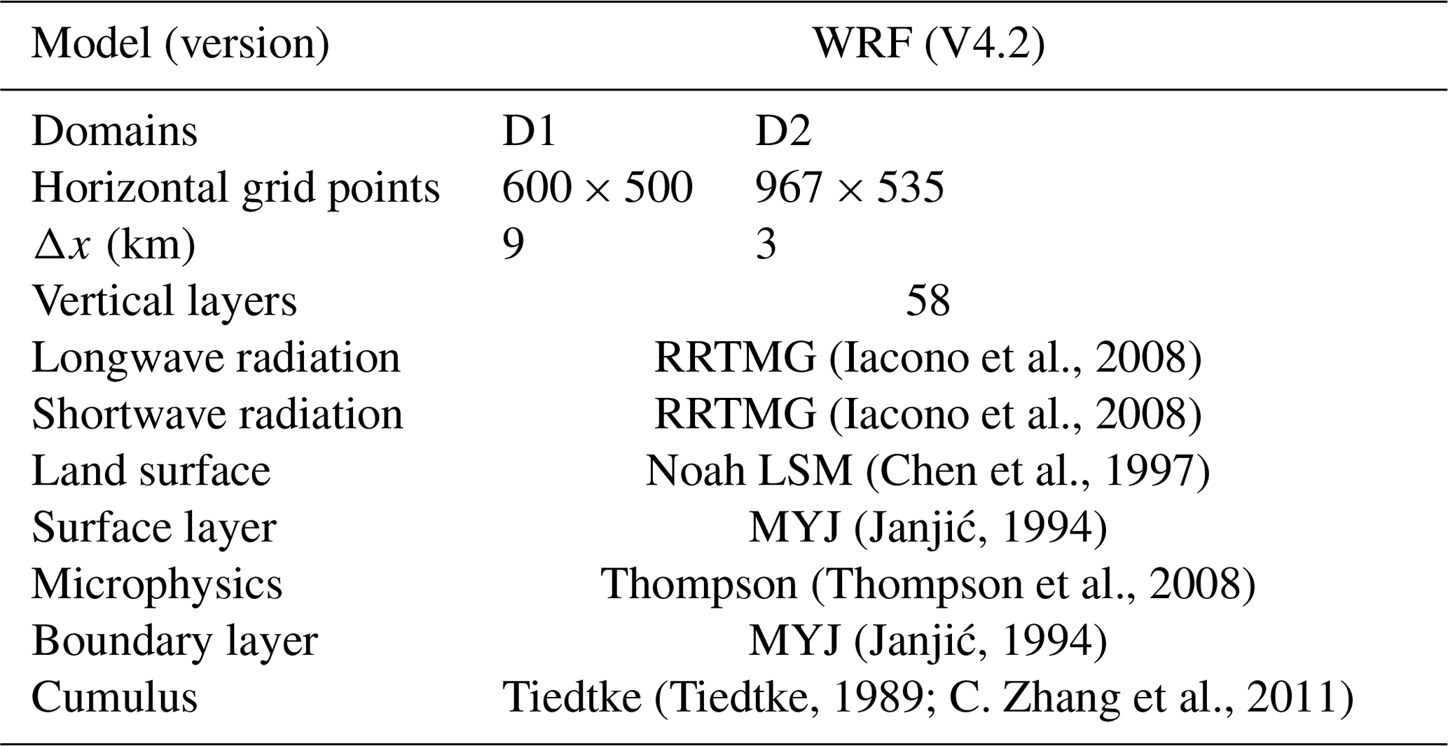
The WRF 4.2 model (Skamarock et al., 2021), developed by the National Center for Atmospheric Research (NCAR), represents a new generation of mesoscale numerical models with numerous applications in research forecasting. We use the WRF model with forcing from the 0.25^∘ × 0.25^∘ Global Forecast System (GFS) model developed by the National Centers for Environmental Prediction (NCEP). We use the first 90 h of the daily GFS forecast initialized at 06:00 UTC (hereafter all time zones are provided as UTC), with 3 h output, to provide initial and boundary conditions for a daily 42 h WRF forecast, analyzing the 18–42 h forecast and discarding the first 18 h as spinup. Surface static data, such as terrain, soil data, and vegetation coverage, are derived from the Moderate Resolution Imaging Spectroradiometer (MODIS) satellite with a resolution of 15 s (approximately 500 m). Incorporating a two-layer grid nesting configuration, the forecast area is illustrated in Fig. 1. The WRF configuration process is detailed in Table 1. Given that the timescale of the meteorological station data in the study area is 1 h, the forecast data time interval of the WRF model is also set to 1 h. As a widely used numerical weather forecast model, the WRF model is suitable for weather studies from a few meters to several thousand kilometers. Therefore, this paper uses the WRF model to predict 10 m wind speed as the input factor for the error correction model.

Table 1 WRF configuration scheme.

2.2.2 Variational mode decomposition

As a new filtering method, VMD is robust in feature selection. The VMD algorithm decomposes a time series signal into several intrinsic mode functions (Isham et al., 2018). The sum of the modes equals the original signal, and the sum of the bandwidths is the smallest. The analysis signal is calculated using the Hilbert transform to estimate the modal bandwidth. The optimization model is described as

$$\begin{array}{}\text{(1)}& \left\{{\min }_{\left\{u_k\right\},\left\{{\mathit{\omega }}_k\right\}}\left\{\sum _{k=\mathrm{1}}^K\left|\right|{\left.{\partial }_t\left[\left(\mathit{\delta }\left(t\right)+{\displaystyle \frac{j}{\mathit{\pi }t}}\right)u_k\left(t\right)\right]e^{-j{\mathit{\omega }}_{k}t}\right|}_{\mathrm{2}}^{\mathrm{2}}\right\}\mathrm{s}.\mathrm{t}.\sum _{k=\mathrm{1}}^K{u}_k=v,\right.\end{array}$$

where K is the total number of modes; u_k is the decomposed kth mode; w_k is the corresponding center frequency; and v is the time series signal, representing the wind speed sequence predicted by the WRF model in this study.

The above-constrained problem can be transformed into an unconstrained problem using the Lagrangian function:

$$\begin{array}{}\text{(2)}& \begin{array}{rl}L& \left(\left\{u_k\right\},\left\{{\mathit{\omega }}_k\right\},\mathit{\lambda }\right)={\mathit{\omega }}_k^{n+\mathrm{1}}\\ & ={\displaystyle \frac{{\int }_{\mathrm{0}}^{\mathrm{\infty }}\mathit{\omega }{\left|{\widehat{u}}_k\left(\mathit{\omega }\right)\right|}^{\mathrm{2}}\mathrm{d}\mathit{\omega }}{{\int }_{\mathrm{0}}^{\mathrm{\infty }}{\left|{\widehat{u}}_k\left(\mathit{\omega }\right)\right|}^{\mathrm{2}}\mathrm{d}\mathit{\omega }}}\sum _{k=\mathrm{1}}^K\left|\right|{\partial }_t\left[\left(\mathit{\delta }\left(t\right)+{\displaystyle \frac{j}{\mathit{\pi }t}}\right)u_k\right(t)\\ & \times ]e^{-j{\mathit{\omega }}_{k}t}\mathrm{|}{\mathrm{|}}_{\mathrm{2}}^{\mathrm{2}}+|\left|v\right(t)-\sum _{k=\mathrm{1}}^K{u}_k(t)\mathrm{|}{\mathrm{|}}_{\mathrm{2}}^{\mathrm{2}}+〈\mathit{\lambda }\left(t\right),v\left(t\right)-\sum _{k=\mathrm{1}}^K{u}_k\left(t\right)〉,\end{array}\end{array}$$

where α is the penalty parameter and λ(t) is the Lagrange multiplier.

Then we update u_k, w_k, and λ using the alternating direction method of the multiplier:

$$\begin{array}{}\text{(3)}& {\displaystyle }{\widehat{u}}_k^{n+\mathrm{1}}\left(\mathit{\omega }\right)={\displaystyle \frac{\widehat{v}\left(\mathit{\omega }\right)-\sum _{i\ne k}{\widehat{u}}_i\left(\mathit{\omega }\right)+\frac{\widehat{\mathit{\lambda }}\left(\mathit{\omega }\right)}{\mathrm{2}}}{\mathrm{1}+\mathrm{2}\mathit{\alpha }{\left(\mathit{\omega }-{\mathit{\omega }}_k\right)}^{\mathrm{2}}}},\text{(4)}& {\displaystyle }{\mathit{\omega }}_k^{n+\mathrm{1}}={\displaystyle \frac{{\int }_{\mathrm{0}}^{\mathrm{\infty }}\mathit{\omega }{\left|{\widehat{u}}_k\left(\mathit{\omega }\right)\right|}^{\mathrm{2}}d\mathit{\omega }}{{\int }_{\mathrm{0}}^{\mathrm{\infty }}{\left|{\widehat{u}}_k\left(\mathit{\omega }\right)\right|}^{\mathrm{2}}\mathrm{d}\mathit{\omega }}},\text{(5)}& {\displaystyle }{\widehat{\mathit{\lambda }}}^{n+\mathrm{1}}\left(\mathit{\omega }\right)={\widehat{\mathit{\lambda }}}^n\left(\mathit{\omega }\right)+\mathit{\tau }\left[\widehat{v}\left(\mathit{\omega }\right)-\sum _{k=\mathrm{1}}^K{\widehat{u}}_k^{n+\mathrm{1}}\left(\mathit{\omega }\right)\right],\end{array}$$

where τ is the update parameter.

When the accuracy (left side of the following expression) meets the following condition, u_k, w_k, and λ would stop updating:

$$\begin{array}{}\text{(6)}& \sum _{k=\mathrm{1}}^K{\displaystyle \frac{\left|\right|{\widehat{u}}_k^{n+\mathrm{1}}-{\left.{\widehat{u}}_k^n\right|}_{\mathrm{2}}^{\mathrm{2}}}{\left|\right|{\widehat{u}}_k^n\mathrm{|}{\mathrm{|}}_{\mathrm{2}}^{\mathrm{2}}}}<\mathit{\epsilon },\end{array}$$

where ε is the tolerance of the convergence criterion.

The VMD algorithm is implemented to decompose the wind speed signal predicted by the WRF model. When using multiple sub-signals instead of the original signal, more features of the wind speed can be obtained. Therefore, it is beneficial to improve the prediction accuracy when using the sub-signal as input to the error correction model (Xu et al., 2021; Li et al., 2022).

2.2.3 Principal component analysis

Subsequences obtained by VMD usually have several illusory components. Using PCA to extract the principal components of subsequences increases the number of features input into the model and reduces the dimension of the data decomposed by VMD. When principal components (PCs) are used as the input of the error prediction algorithm, the PCs fully reflect the characteristics of the subsequence and reduce the model complexity. The PCs y_k, k=1, 2, …, K of the subsequence matrix U and the cumulative contribution rate η_n of the first n principal components are expressed as

$$\begin{array}{}\text{(7)}& {\displaystyle }{y}_k=c_k^{\prime }\mathbf{U},\text{(8)}& {\displaystyle }{\mathit{\eta }}_n={\displaystyle \frac{\sum _{k=\mathrm{1}}^n{\mathit{\lambda }}_k}{\sum _{k=\mathrm{1}}^K{\mathit{\lambda }}_k}},\end{array}$$

where c_k is the corresponding characteristic unit vector, with k=1, 2, …, K; λ_k is the characteristic root, with ${\mathit{\lambda }}_{\mathrm{1}}\ge {\mathit{\lambda }}_{\mathrm{2}}\ge \mathrm{\dots }\ge {\mathit{\lambda }}_K$.

2.2.4 Evaluation indicators

There are many commonly used predictive effect evaluation indicators. This article uses the following evaluation indicators: correlation coefficient (R), root mean square error (RMSE), mean absolute error (MAE), relative root mean square error (rRMSE), relative mean absolute error (rMAE), and forecasting accuracy (FA). Six error indicators are used to evaluate the correction results of short-term wind speed forecasts of wind farms. The formula for calculating the error index is as follows:

$$\begin{array}{}\text{(9)}& {\displaystyle }R={\displaystyle \frac{\sum _i^n\left(y_i-\stackrel{\mathrm{‾}}{y}\right)\left({\widehat{y}}_i-\stackrel{\mathrm{‾}}{\widehat{y}}\right)}{\sqrt{\sum _{i=\mathrm{1}}^n{\left(y_i-\stackrel{\mathrm{‾}}{y}\right)}^{\mathrm{2}}}\sqrt{\sum _{i=\mathrm{1}}^n{\left({\widehat{y}}_i-\stackrel{\mathrm{‾}}{\widehat{y}}\right)}^{\mathrm{2}}}}},\text{(10)}& {\displaystyle }\mathrm{RMSE}=\sqrt{{\displaystyle \frac{\mathrm{1}}{n}}\sum _{i=\mathrm{1}}^n{\left({\widehat{y}}_i-y_i\right)}^{\mathrm{2}}},\text{(11)}& {\displaystyle }\mathrm{MAE}={\displaystyle \frac{\mathrm{1}}{n}}\sum _{i=\mathrm{1}}^n\left|{\widehat{y}}_i-y_i\right|,\text{(12)}& {\displaystyle }\mathrm{rRMSE}=\left[\sqrt{{\displaystyle \frac{\mathrm{1}}{n}}\sum _{i=\mathrm{1}}^n{\left({\widehat{y}}_i-y_i\right)}^{\mathrm{2}}}/\left({\displaystyle \frac{\mathrm{1}}{n}}\sum _{i=\mathrm{1}}^n{y}_i\right)\right]\times \mathrm{100}\mathit{\%},\text{(13)}& {\displaystyle }\mathrm{rMAE}=\left({\displaystyle \frac{\mathrm{1}}{n}}\sum _{i=\mathrm{1}}^n\left|{\widehat{y}}_i-y_i\right|/\left({\displaystyle \frac{\mathrm{1}}{n}}\sum _{i=\mathrm{1}}^n{y}_i\right)\right)\times \mathrm{100}\mathit{\%},\text{(14)}& {\displaystyle }\mathrm{FA}=N_r/N_f.\end{array}$$

Among them, n represents the number of samples, ${\widehat{y}}_i$ represents the ith predicted value, and y_i represents the ith actual value; N_r represents the number of wind speed absolute errors not greater than 1 m s⁻¹, and N_f represents the number of research samples.

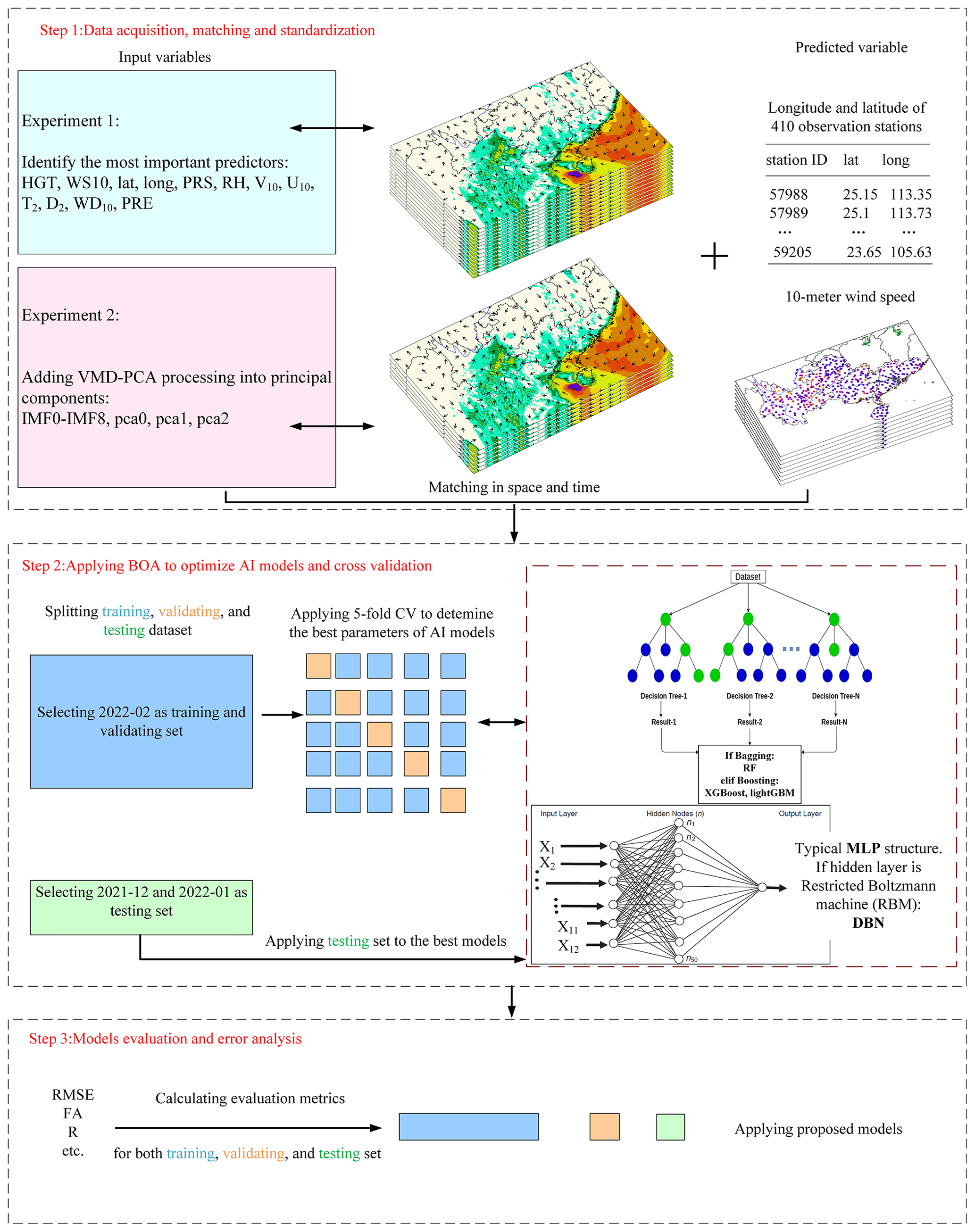
Figure 2 Flowchart of the artificial intelligence (AI) model used to correct WRF-predicted wind speeds in the two main experimental pathways.

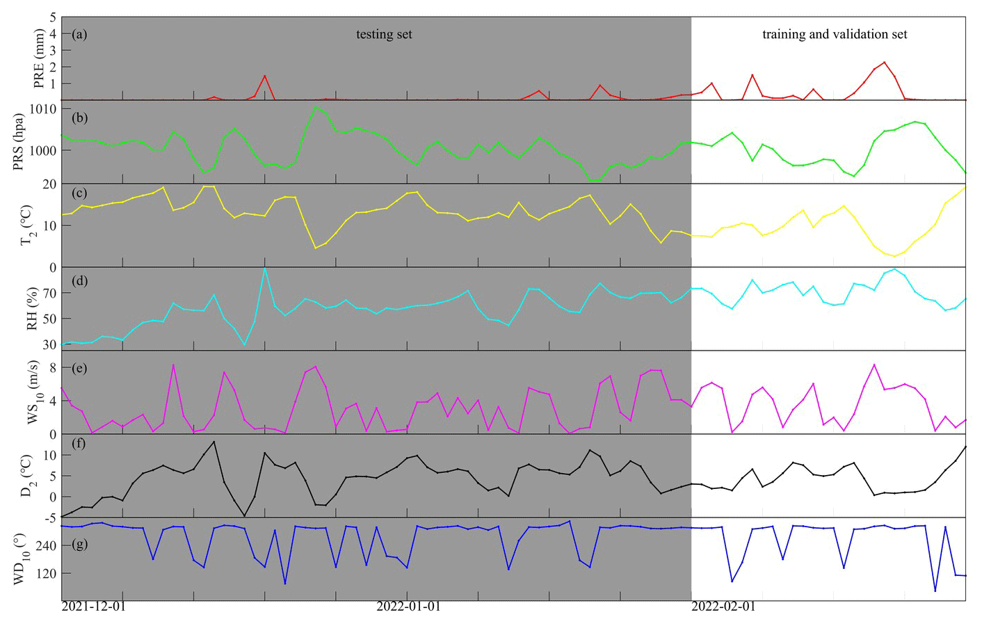
Figure 3 Daily average hourly rainfall (a), surface pressure (b), 2 m temperature (c), 2 m relative humidity (d), 10 m wind speed (e), 2 m dew point temperature (f), and 10 m wind direction (g) which are located at Guangdong Lechang Station from 1 December 2021, to 28 February 2022. (February 2022 represents the training and verification sets, and December 2021 to January 2022 represents the testing set).

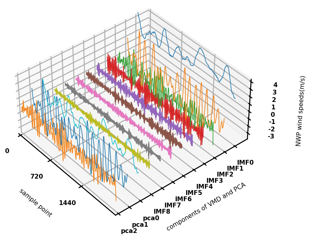
Figure 4 Three-dimensional view of 12 wind speed components after VMD and PCA processing of the 10 m forecast wind speed at Lechang Station in Guangdong from 1 December 2021 to 28 February 2022.

2.2.5 Proposed hybrid forecasting algorithms

This study used five machine learning algorithms to conduct 10 experiments following two main paths. The first path involves increasing the meteorological variables possibly related to wind speed in the forecast field. The correlation between the WRF-predicted 10 m wind speed and the observed wind speed is the highest. The purpose of the second experimental path is using the VMD-PCA algorithm to dig out the hidden wind speed characteristics of the 10 m forecast wind speed, reduce the input of other meteorological factors such as WD₁₀ and D₂, and further prove that the VMD-PCA algorithm is effective before correcting the WRF-predicted wind speed. The overarching goal is to achieve accurate correction of the forecast field wind speed. The flowchart of the artificial intelligence models used to correct the WRF-predicted wind speed for the two main experimental paths is illustrated in Fig. 2 and comprises the following three steps:

•  

  Step 1 – data fusion, cleaning, and standardization. As depicted in Fig. 2, this paper proposes two distinct experimental paths, with the primary difference being the selection of input variables. In experiment 1, as shown in Fig. 2, 12 sets of data are selected from the WRF forecast field, including altitude (HGT), 10 m wind speed (WS₁₀), latitude (lat), longitude (long), surface pressure (PRS), relative humidity (RH), 10 m meridional wind (V₁₀), 10 m zonal wind (U₁₀), 2 m temperature (T₂), 2 m dew point temperature (D₂), 10 m wind direction (WD₁₀), and hourly precipitation (PRE). Experiment 2 derives eight sets of data by reducing the selected WRF field forecast data to include only altitude, 10 m wind speed, latitude, longitude, surface pressure, relative humidity, 2 m temperature, and hourly precipitation. The focus is on unearthing hidden characteristic information of forecast wind speed. In this experiment, the wind speed is decomposed into nine intrinsic mode functions (IMFks; k=0, 1, 2, …, 8) using VMD. Subsequently, a low-dimensional wind speed vector is extracted from the nine IMF components via PCA dimensionality reduction (pca0, pca1, pca2), and all data are concatenated to construct the input factors for the model in experiment 2. The time points in the dataset where missing values are located are eliminated. Experiment 1 (experiment 2) standardizes 12 sets of meteorological elements (8 sets of meteorological elements in Fig. 3, 9 IMF components, and 3 PCA vectors in Fig. 4) and wind speed observation data, respectively. Standardization addresses the issue of varying meteorological factor values during training, which may result in different contributions. In this paper, the 24 h forecast data correspond to the observation data of the subsequent 24 h. The dataset spans from 00:00 on 1 December 2021 to 23:00 on 28 February 2022, totaling 2160 h and encompassing 410 weather stations. Consequently, the original dataset comprises 2160 × 410 samples, with each sample containing 12 meteorological features in experiment 1 and 20 input features in experiment 2. While similar past studies for wind speed correction from NWP models usually use several years for training and at least 1 year for testing, our periods are shorter, but the size of our dataset is sufficient. For example, Sun et al. (2019) used a dataset that contained 1827 d, from January 2012 to December 2016, using 143 grid points with a resolution of 0.5^∘ × 0.5^∘ predicted by ECMWF, followed by 24 features for each sample, with a training set size of 1827 × 143 × 24 for each prediction time. Meanwhile, the size of our training set is about 2160 × 410 × 12. Therefore, even though it only took us a month to train, for this project, we trained millions of data. Second, the training data we used here were obtained through daily operational runs of numerical weather forecasting, so it would have taken several years to get an equal amount of training data.

•  

  Step 2 – BOA optimization of AI models and cross-validation. In this study, the dataset is partitioned into training, validation, and test sets in accordance with the time series. February 2022 serves as the training and validation sets, while December 2021 and January 2022 constitute the test set. The training and validation sets are divided based on 5-fold cross-validation. Both experiments employ five machine learning algorithms (DBN, MLP, RF, XGBoost, and lightGBM) to construct distinct machine learning models. Concurrently, this paper utilizes the BOA algorithm to tune the parameters of all models, except for DBN, resulting in the optimal hyperparameters for each model.

•  

  Step 3 – model evaluation and error analysis. The trained machine learning models are applied to the test set to obtain the revised wind speed data, and ultimately, the accuracy of all models is assessed through the wind speed evaluation index. The ultimate goal here is to identify the best wind speed correction model suitable for the entire year. Accordingly, the generalization of all models is evaluated across other seasonal months of the year, culminating in the selection of the best model.

3 Results

3.1 Experiment 1 evaluation

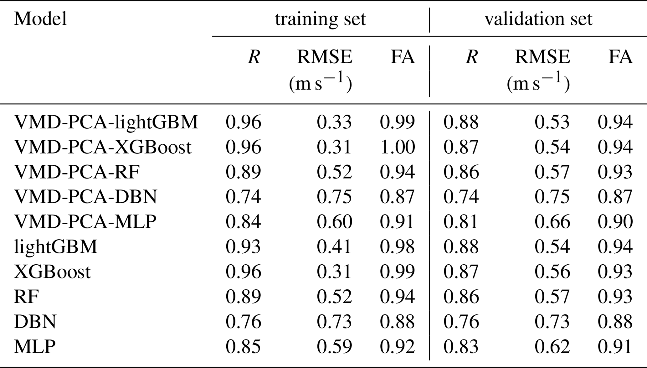
In experiment 1, the BOA optimization algorithm was applied to five AI models to correct the 10 m wind speed forecasted by WRF. There were 12 meteorological element features to establish five different AI models (see Table S1 for the hyperparameters of the five AI models). The training, validation, and testing results for 10 m wind speed are shown in Figs. S1–S5 in the Supplement. It is clear from Table 2 that all models, except the DBN model, can fit the training set data well. The DBN model exhibits the weakest performance on both the training and the validation sets. Alternatively, the lightGBM and XGBoost models demonstrate superior prediction performance on the training set compared to the validation set. The scatters of the training sets of these two models accumulate on the 1:1 diagonal, indicating slight overfitting. As shown in Figs. S1–S5d, f, considering different evaluation indices, the revision effects of the five models in 2 months demonstrate that RMSE in January 2022 is generally lower than in December 2021, FA in January 2022 is generally higher than in December 2021, and R in January 2022 is generally lower than in December 2021. Overall, the prediction performance of the five models in January 2022 surpassed that in December 2021. Furthermore, the lightGBM and RF models exhibited the best performance among the five models in the 2-month test sets, while the DBN model had the least effective correction effect.

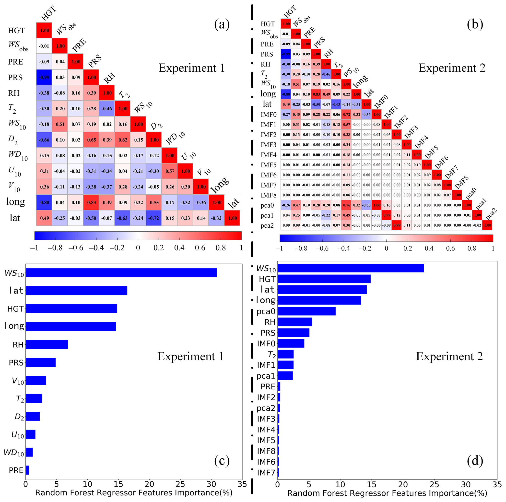
Figure 5 Schematic diagram of correlation coefficients (represented by the WS₁₀ and input variables) and feature importance (calculated by the scikit-learn Python package) for two sets of experiments. Panels (a) and (c) represent experiment 1, and (b) and (d) represent experiment 2.

Table 2 Table of the evaluation indices of wind speed error trained and verified by the 10 models in February 2022.

As illustrated in Fig. 5a, b, WS₁₀ showed the strongest positive correlation with WS_obs, with the highest R of 0.51, which was consistent with the highest variable importance value of 31 % (23 %) in experiment 1 (experiment 2). In addition to WS₁₀, experiment 1 (experiment 2) also had another three dominant variables, namely lat, HGT, and long, with importance values of 16 % (14 %), 15 % (15 %), and 15 % (13 %), respectively. Meanwhile, in experiment 2, IMF0 and pca0 generated by the VMD-PCA algorithm have a good importance value of 9 % and 4 %, and the R values of them with WS_obs are as high as 0.47 and 0.45.

Concerning the importance of RF characteristics (Fig. 5a, c), it is indisputable that the 10 m wind speed predicted by WRF plays a dominant role in correcting the actual wind speed. The ones following are latitude, longitude, and topographic height, which represent spatial geographic information, and the actual wind speed is closely related to geographic information. Subsequently, relative humidity is of lesser importance. The distribution of the humidity field typically correlates with the movement of the atmosphere, which is also closely related to wind speed. Certain meteorological elements, such as rainfall, 2 m dew point temperature, and 2 m temperature, contribute less importance.

3.2 Experiment 2 evaluation

Experiment 2 builds upon experiment 1, concentrating on the predicted 10 m wind speed by the WRF model. We use the VMD algorithm to decompose the predicted wind speed into nine components and use the PCA algorithm to extract the main three principal components. In the RF feature importance analysis (Fig. 5b, d), it is evident that the VMD algorithm can decompose IMF0 and IMF1, with contributions surpassing those of 2 m temperature and precipitation, respectively. The importance of the pca0 component, after PCA extraction, reaches up to 8 %. What is particularly interesting is that in the correlation analysis, the correlation values between the IMF0 and pca0 components and the actual wind speed are 0.50 and 0.51, which are second only to the forecasted wind speed.

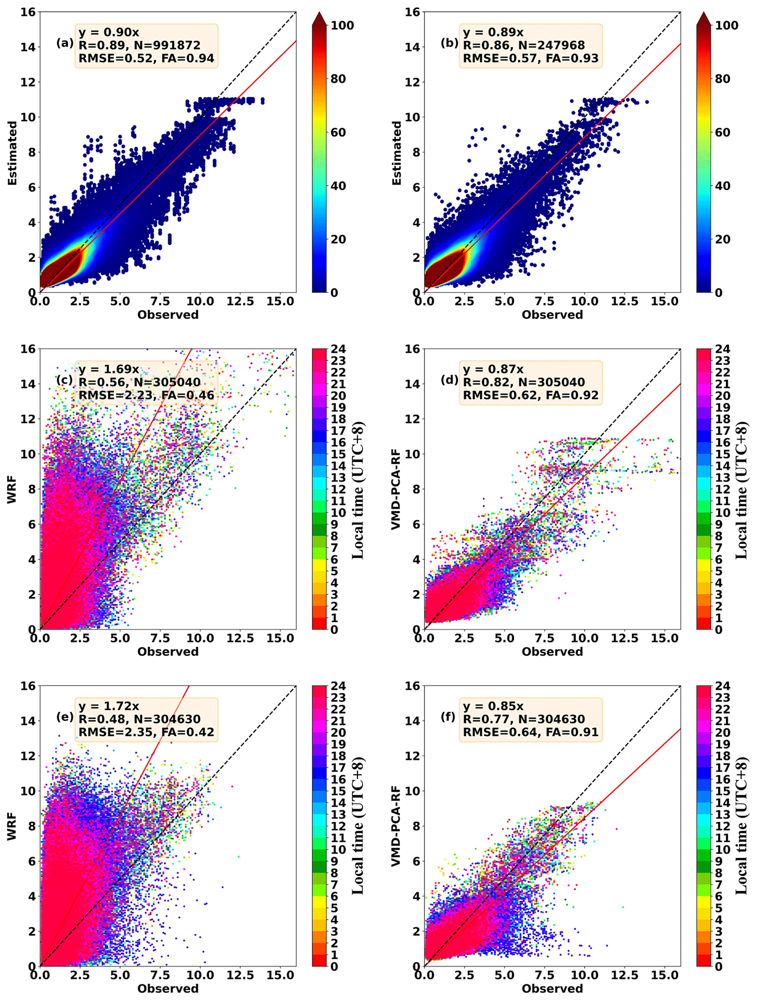
Figure 6 The scatter density map compared with the actual 10 m wind speed: (a) 10-fold cross-validation training set of the VMD-PCA-RF model in February 2022 and (b) 10-fold cross-validation validation set of the VMD-PCA-RF model in February 2022. The 24 h scatter map compared with the actual 10 m wind speed: (c) WRF forecasts in December 2021, (d) the VMD-PCA-RF model forecasts in December 2021, (e) WRF forecasts in January 2022, and (f) the VMD-PCA-RF model forecasts in January 2022.

From the indices (RMSE, FA, R) of the training and validation sets shown in Table 2, in comparison to the above five artificial intelligence methods, the training results of VMD-PCA-DBN are relatively inferior. VMD-PCA-lightGBM and VMD-PCA-XGBoost models still train the processed data effectively. According to the scatter density figure (Figs. 6a, 7a), the scatters are relatively concentrated on the 1:1 line. From the indicators (RMSE, FA, R) of the testing set shown in Figs. S6–S8d, f and 6–7d, f, the test results of the five models in experiment 2 in December 2021 and January 2022 show that the error indices of RMSE and FA of each model exhibit a minimal difference in 2 months. Nonetheless, disregarding the R results, the performance of the five models in December 2021 is inferior to that in January 2022. The diurnal variation scatterplot of 2 months is tested. As is shown in Figs. S6–S8d, f and 6–7d, f, the red scatters represent the nighttime wind speed, which is more concentrated on the 1:1 line. In contrast, the blue scatters represent the afternoon wind speed, which is slightly away from the 1:1 line. This suggests that the correction effect of the five models (VMD-PCA-lightGBM, VMD-PCA-XGBoost, VMD-PCA-RF, VMD-PCA-DBN, and VMD-PCA-MLP) exhibits a noticeable diurnal variation.

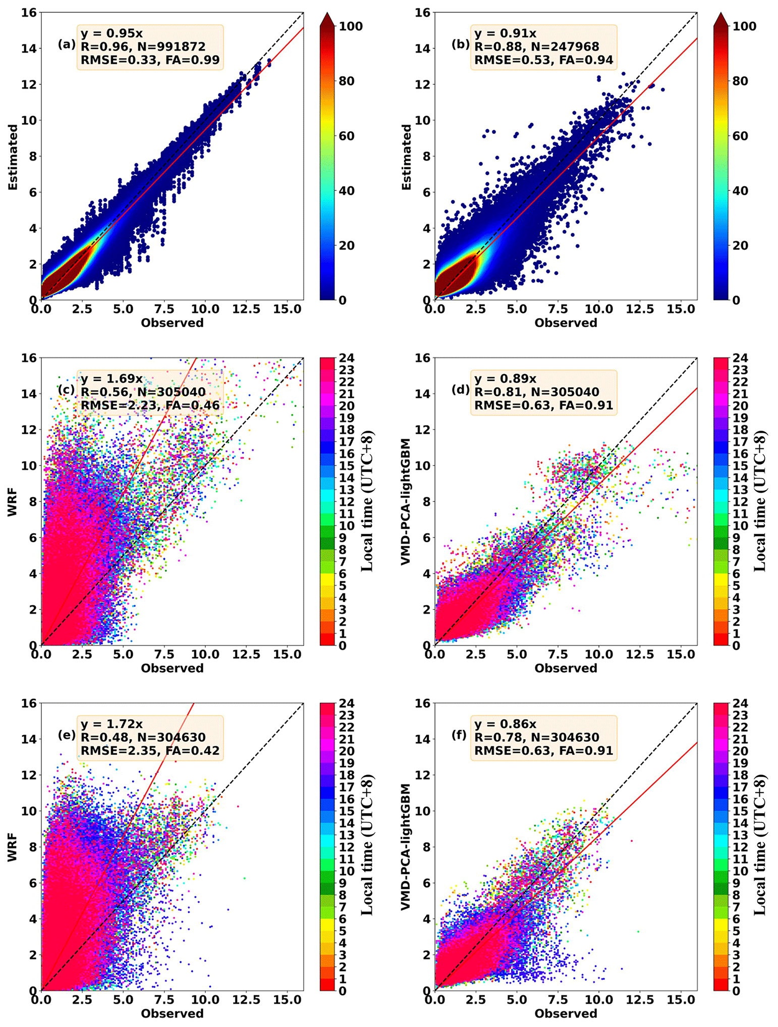
Figure 7 The scatter density map compared with the actual 10 m wind speed: (a) 10-fold cross-validation training set of the VMD-PCA-lightGBM model in February 2022 and (b) 10-fold cross-validation validation set of the VMD-PCA-lightGBM model in February 2022. The 24 h scatter map compared with the actual 10 m wind speed: (c) WRF forecasts in December 2021, (d) the VMD-PCA-lightGBM model forecasts in December 2021, (e) WRF forecasts in January 2022, and (f) the VMD-PCA-lightGBM model forecasts in January 2022.

3.3 Comparison of the two experiments

Firstly, all 10 models effectively corrected the 10 m wind speed forecasted by WRF. Tables S2 and S3 represent the evaluation indices of wind speed errors predicted by the 10 models in December 2021 and January 2022. From the two tables, it is evident that the VMD-PCA-RF and VMD-PCA-lightGBM models have the best performance in December 2021 and January 2022, respectively, with the most comprehensive performance of the forecast indicators. The MAE, RMSE, rMAE, rMAE, and FA for the two models VMD-PCA-RF (VMD-PCA-lightGBM) were 0.46 m s⁻¹ (0.45 m s⁻¹), 0.62 m s⁻¹ (0.63 m s⁻¹), 37.36 % (34.75 %), 50.39 % (48.65 %), and 91.79 % (91.49 %) in December 2021 (January 2022). Additionally, based on the analysis of the Taylor chart (Fig. 8e, f) of the 10 models in Fig. 8, it can also be seen that the scatter distance of VMD-PCA-RF and VMD-PCA-lightGBM models is the closest to the observed dotted black line and the black triangle position. The two models show that the standard deviation is close to the observed wind speed, with the lowest RMSE and the highest R. Secondly, in the comparison of cumulative probability distributions, all models passed Kolmogorov's 5 % confidence interval test when the interval of wind speed is 0.5 m s⁻¹ (Fig. 8a, d). However, when the interval of wind speed is 0.2 m s⁻¹ (Fig. 8b, e), the VMD-PCA-lightGBM model deviated from Kolmogorov's 5 % confidence interval detection in December 2021. This indicates that the VMD-PCA-RF model has a better predictive effect than the VMD-PCA-lightGBM model in December 2021 when the actual wind speed is within the range of 0.4–0.8 m s⁻¹.

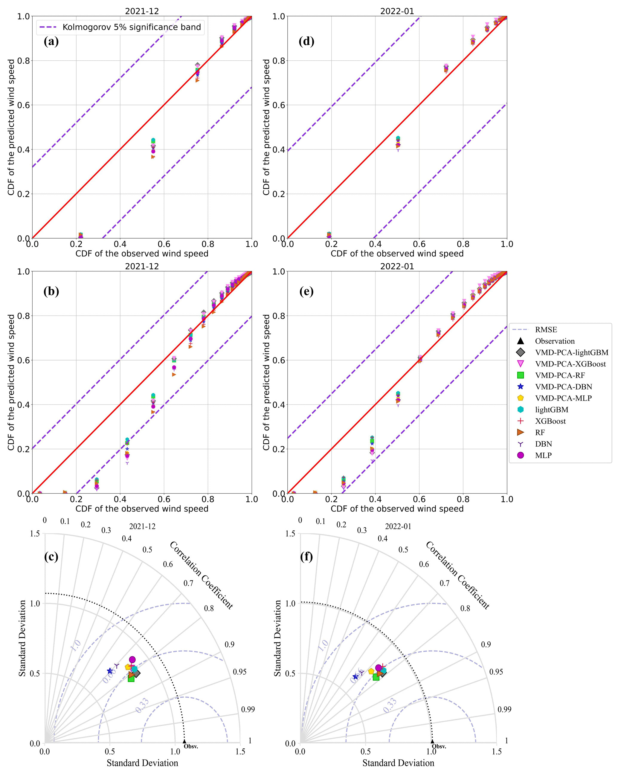
Figure 8 The cumulative distribution probability scatterplots of the actual wind speed and the predicted wind speed of the 10 models in wind speed intervals of 0.5 m s⁻¹ (a represents December 2021, d represents January 2022) and 0.2 m s⁻¹ (b represents December 2021, e represents January 2022), respectively; Taylor distribution map (c represents December 2021, f represents January 2022).

3.4 Spatial–temporal variations in the best models

Based on our comparative analysis results, we conclude that the best-performing combination models in December 2021 and January 2022 are VMD-PCA-RF and VMD-PCA-lightGBM, respectively. Figures 9 and S9 show the diurnal variation corrections of the two best models for a given month, as well as the diurnal variation of wind speed in the original WRF forecast. The wind speed of the original WRF numerical weather forecast shows a noticeable overestimation, which is confirmed in Fig. 7c and e. The scatters of the WRF forecast predominantly deviate towards the upper-left corner, with relatively low correlation coefficients, 0.56 and 0.23, respectively. Furthermore, the wind speed forecast by WRF displays obvious diurnal variation traits, characterized by large errors between the afternoon and evening, specifically between 11:00 and 20:00 (Figs. 9a, S9a). Moreover, the actual average wind speed in January 2022 deviates from the range of 1 standard deviation of the WRF forecast wind speed at 17:00 and 18:00 (Fig. S9a). This demonstrates that the wind speed forecast by WRF is inaccurate and exhibits substantial diurnal variation errors.

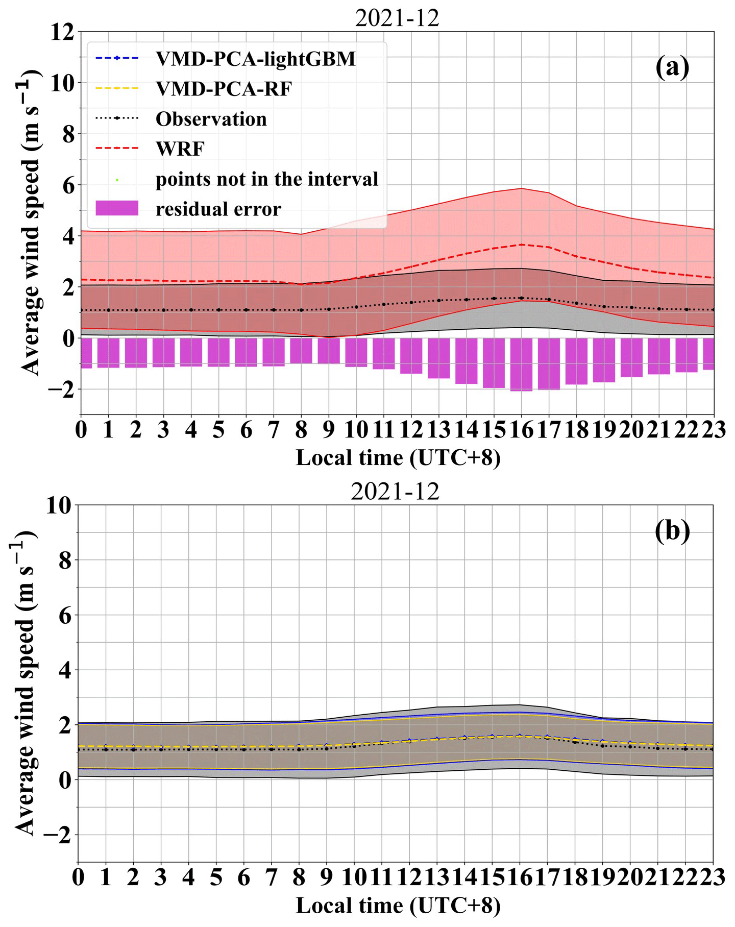
Figure 9 VMD-PCA-lightGBM, VMD-PCA-RF, and WRF daily variation in predicted and actual wind speeds in December 2021. (The shaded areas represent an interval of 1 standard deviation, which is a 68 % confidence interval).

After the best model was corrected, the error in diurnal variation was significantly reduced (Figs. 9b, S9b). First, the average wind speed corrected by the best model is essentially consistent with the actual average wind speed curve, with minimal error and no diurnal variation. Second, the 1 standard deviation range of the corrected and actual wind speeds is also well matched, indicating that the corrected and actual wind speed distributions are consistent. The correction effect at 16:00 and 17:00 on January 2022 is suboptimal, which may be due to the insufficient generalization of the training model and the excessive fluctuation of the actual wind speed at these two time points.

The FA (Figs. 10a, S10a) and RMSE (Figs. 10b, S10b) distribution of the WRF forecast 10 m wind speed at 410 stations in the five southern provinces shows that the 10 m wind speed prediction effect of the WRF model in Yunnan is superior to that in the other four provinces. In the regions of Hainan, Guangxi, and Guangdong, the number of sites with an RMSE for 10 m wind speed forecast in December 2021 ranging from 5.6 to 6.0 m s⁻¹ was significantly higher than in January 2022, especially in coastal areas (Figs. 10b, S10b). In the Yunnan area, the FA of most WRF forecast station 10 m wind speeds exceeds 40 %, and the RMSE value is mostly below 2.4 m s⁻¹. Conversely, in other regions, such as Guangxi, Guangdong, and Hainan, the terrain is relatively flat. The FA of the 10 m wind speed forecast by WRF is as low as 30 % at some stations, and the RMSE reaches up to 5.4 m s⁻¹. However, after the VMD-PCA-RF and VMD-PCA-lightGBM models are corrected, the FA of most stations in the five southern provinces is as high as 90 %, and the RMSE is as low as 0.6 m s⁻¹. Moreover, in Guangxi, Guangdong, and Hainan, where the WRF forecast effect is subpar, the accuracy of the corrected 10 m wind speed by VMD-PCA-RF (VMD-PCA-lightGBM) is significantly improved.

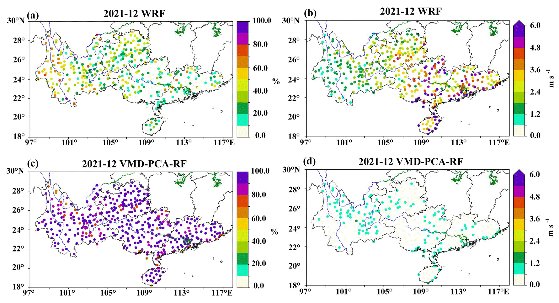
Figure 10 FA (a, c) and RMSE (b, d) distribution maps of the VMD-PCA-RF and WRF models at 410 sites in five southern provinces in December 2021.

4 Discussion

4.1 The effects of BOA-VMD-PCA

It is shown in Table S1 that the hyperparameters of the 10 models in the two experiments are different. Since the DBN model is not added to the scikit-learn Python learning package, it is challenging to use the BOA algorithm for tuning parameters. Apart from the DBN model, all the other models are optimized using the BOA algorithm. From the various evaluation indicators in Tables S2 and S3, the DBN model, which does not use the BOA algorithm to adjust the model parameters to obtain an optimal parameter configuration, yields the worst prediction results in December 2021 and January 2022. Moreover, studies (Xiong et al., 2022) have also shown that BOA can further improve the model's prediction accuracy by configuring optimal hyperparameters. The hyperparameters, such as the number of neurons and learning rate in the hidden layer, significantly impact the model's performance. When the same model is applied to different datasets of two experiments, the BOA adaptively obtains the optimal combination of hyperparameters, overcoming the limitations of manual parameter adjustment (Guo et al., 2021). This suggests that the selection of model hyperparameters introduces considerable uncertainty in our prediction results. Therefore, the choice of optimization model parameters represents one source of uncertainty in the correction results, which entails the complexity of parameter selection. However, a more advanced parameter tuning method, such as the BOA tuning algorithm, is essential.

The VMD is used to obtain unknown but meaningful features hidden in the 10 m wind speed sequences predicted using WRF models (Li et al., 2022). In addition, the PCA can extract important components of anemometer subsequences. When the stationary subsequence serves as an input to the error correction model, it contains more valuable information than the previous non-stationary wind speed sequences (Xu et al., 2021).

The complexity of the input factors in this study is one of the sources of uncertainty in the process of correcting WRF prediction results. The input factors of the two experiments are not identical. In the second set of experiments, the input of meteorological factors is reduced based on the first set of experiments, while component information of the 10 m wind speed predicted by WRF is increased. Multiple wind speed components processed by VMD-PCA and noise reduction are introduced. Among them, the importance of introduced pca0 and IMF0 is approximately 5 %. In the 13-month test sets, the correction accuracy of experiment 2 is no less than the results of experiment 1 (Figs. S11, 12), indicating that the 10 m wind speed components introduced by VMD-PCA contribute positively to the correction results.

4.2 RF feature importance

To further understand the feature importance ranking of the RF models, we divided the model prediction results and actual wind speeds of the 410 stations into 20 equal parts according to terrain height above sea level (Fig. 11). First of all, the actual wind speed in December 2021 and January 2022 varies with the height of the station, showing that the lower the height of the station, the more significant the change in wind speed. This relationship is associated with the wind speed profile of the atmosphere, where wind speed increases as height decreases. Secondly, the wind speed during the day is generally greater than the wind speed at night, which is related to the turbulent motion of the atmosphere during the day. Solar radiation causes the atmosphere to mix, resulting in convective movement. The 10 m wind speed at night is affected by the cooling radiation of the surface, and the atmosphere is relatively stable.

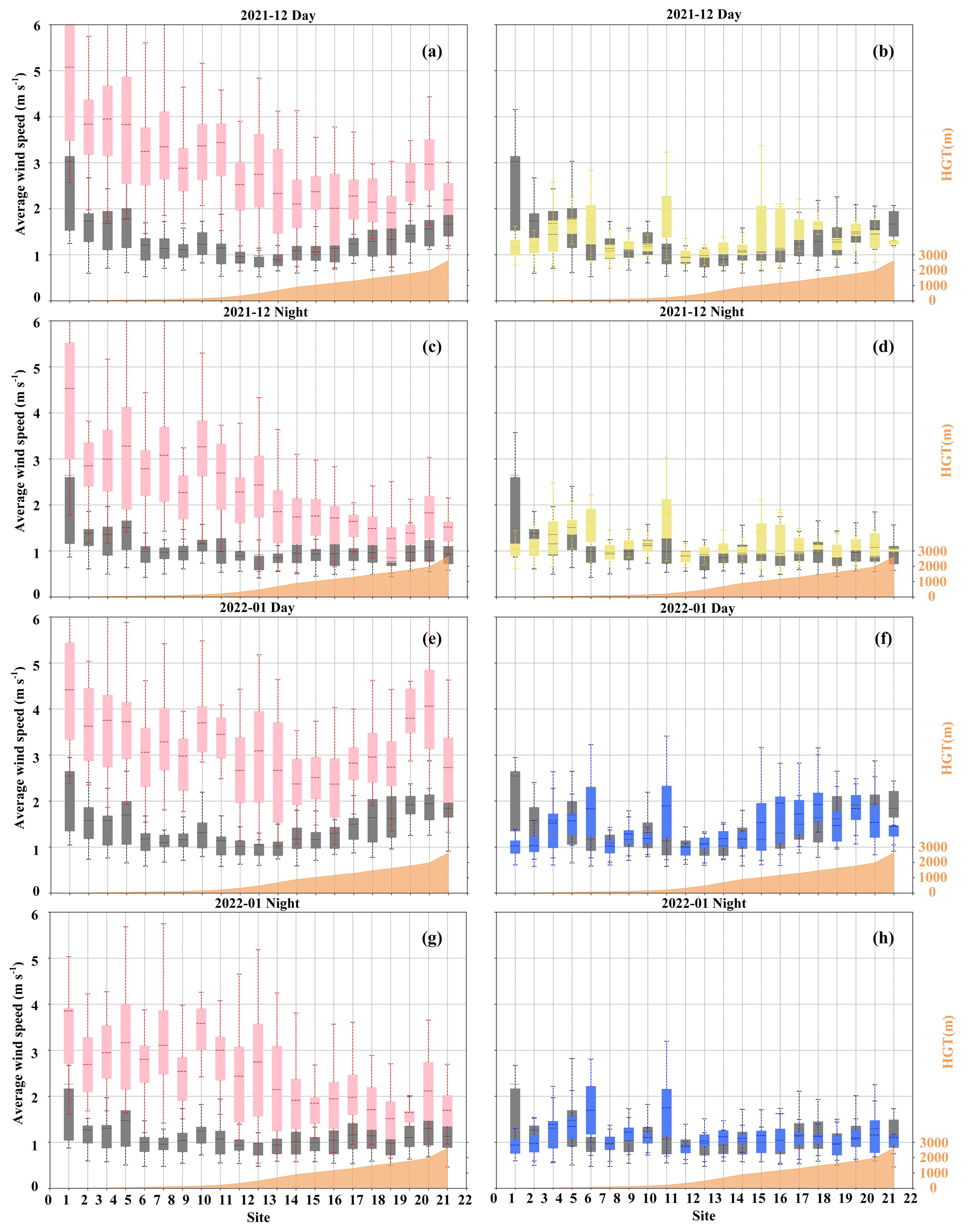
Figure 11 The boxplots of the predicted wind speeds of the VMD-PCA-RF (yellow), VMD-PCA-lightGBM (blue), and WRF (pink) models at 20 stations at different height intervals and the boxplots of the actual wind speeds (gray).

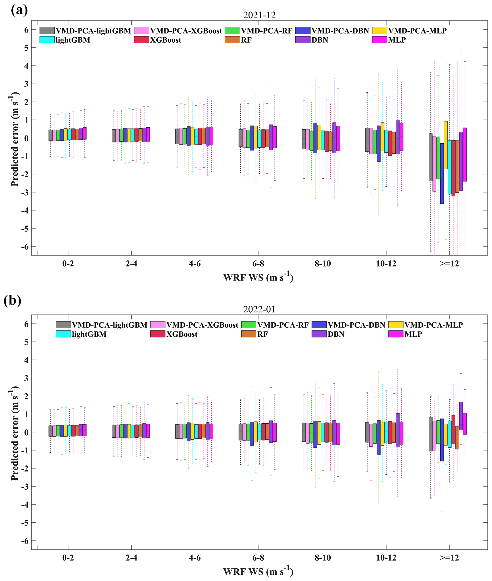
The 10 m wind speed predicted by WRF has the highest feature importance in the correction process of the RF models. Input factors with distinct geographic information, such as latitude, longitude, and height, rank highly in feature importance. Similarly, when Sun et al. (2019) used machine learning to correct the 10 m wind speed predicted by the numerical weather prediction model ECMWF, the characteristic weight of the 10 m wind speed predicted by the model was the highest, followed by the sea–land factor. Moreover, as the 10 m wind speed forecast by WRF increased, the instability of the 10 m wind speed corrected by the 10 machine learning models gradually increased, and the correction accuracy gradually decreased (Fig. 12). This partly explains the higher importance of the 10 m wind speed forecast by WRF.

Figure 12 The prediction error boxplots of 10 models in different WRF prediction intervals.

With 1 km as the center, the measured 10 m wind speed is more variable in areas where the station terrain height increases or decreases. However, the pink box of the 10 m wind speed predicted by WRF becomes wider as the station terrain height decreases (Fig. 11). The distance between the gray box and the pink box is greater as the station terrain height decreases. It shows that the 10 m wind speed predicted by WRF has less accuracy with the station terrain height decreases. The VMD-PCA-RF and VMD-PCA-lightGBM models significantly reduce the variability in the 10 m wind speed predicted by WRF. When the height of the station increases or decreases at 1 km, the correction intensity tends to increase gradually. This further explains the higher importance of the height factor in the RF model training.

4.3 Stability analysis of the proposed models

In order to identify the best model of the five southern provinces and assess the model's stability, we evaluated all 10 models over 13 different months. Figure 13 shows the evaluation histogram of the 10 m wind speed predicted by the 10 models in experiment 1 and experiment 2, as well as the actual wind speed in various months. Meanwhile, Figs. S11 and S12 can more effectively illustrate the daily changes in the revised results of the 10 models in 13 different months. As shown in Fig. 13, the evaluation indices of the model trained in experiment 2, after VMD-PCA processing, outperform those of the model trained in experiment 1. The RF model demonstrates exceptional robustness, while the MLP model exhibits the poorest performance. VMD-PCA-RF evaluation indices are relatively stable across the 13 months, with a correlation coefficient R above 0.6, FA above 85 %, MAE below 0.6 m s⁻¹, RMSE below 0.8 m s⁻¹, rMAE below 60 %, and rRMSE below 75 %. However, the robustness of the VMD-PCA-lightGBM and VMD-PCA-XGBoost models is inferior to that of the VMD-PCA-RF model, with all six evaluation indices performing worse than the VMD-PCA-RF model as the seasons and months change. In general, VMD-PCA-lightGBM is the superior wind speed correction model for the winter, and VMD-PCA-RF performs the best throughout the entire year in the five southern provinces. In cases where ample machine CPU and other hardware resources, as well as training time, are available, we recommend using VMD-PCA-lightGBM for modeling each season. However, when dealing with limited resources such as a laptop and constrained training time, we recommend using VMD-PCA-RF to train data for a single month, as this yields the most robust correction results.

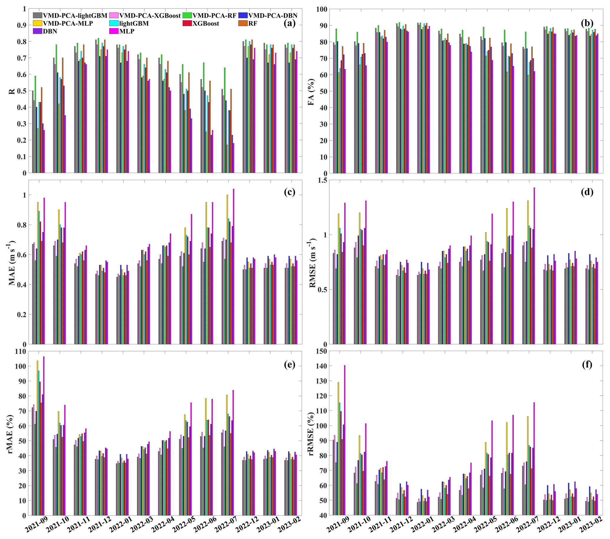
Figure 13 Evaluation histograms of 10 m wind speed predicted by the 10 models in different months in experiment 1 and experiment 2 (a, b, c, d, e, and f represent R, FA (%), MAE (m s⁻¹), RMSE (m s⁻¹), rMAE (%), and rRMSE (%), respectively).

5 Conclusions

In an effort to enhance the wind speed prediction performance for wind farms, this study developed a WRF-based multi-step wind speed prediction model. A hybrid error correction strategy combining BOA, VMD, PCA, and RF (lightGBM) is proposed to increase the accuracy of WRF simulations. The first group of experiments used various meteorological elements as input factors in a control experiment. In the second group of experiments, the wind speed sequence predicted by the WRF model was decomposed into multiple IMFs using the VMD algorithm for feature extraction. A principal component analysis method is used to extract meaningful principal components from these subsequence IMFs to improve computational efficiency. In the error correction model, RF (lightGBM) and other algorithms are used to train the relationship between different input factors and the actual wind speed error, respectively.

Through a case analysis of 410 stations in five southern provinces in China, the following conclusions can be drawn: (1) the machine learning models tuned by the BOA-VMD-PCA algorithm exhibit a positive impact on wind speed error correction; (2) feature importance analysis revealed that the top eight contributing factors for correcting WRF-forecasted wind speed include WRF forecast 10 m wind speed (WS₁₀), latitude, longitude, altitude, pca0 (pca0 physically represents the lowest-frequency wind speed series after PCA treatment of all IMFks (k=0, 1, 2, …, 8) sub-series with reduced dimension), humidity, pressure, IMF0 (IMF0 physically represents the wind speed stationary series with a specific lowest center frequency after the original wind speed series has been processed by VMD); (3) VMD-PCA-RF and VMD-PCA-lightGBM are the most suitable wind speed correction algorithms for December 2021 and January 2022, respectively. The MAE, RMSE, FA, rMAE, rRMSE, and R of the corrected wind speed and the actual wind speed are 0.46 (0.45), 0.62 m s⁻¹ (0.63 m s⁻¹), 37.36 % (34.75 %), 50.39 % (48.65 %), 91.79 % (91.49 %), and 0.82 (0.78); and (4) the proposed wind speed correction model (VMD-PCA-RF) demonstrates the highest prediction accuracy and stability in the five southern provinces in nearly a year and at different heights. VMD-PCA-RF evaluation indices for 13 months remain relatively stable: R is above 0.6, FA is above 85 %, MAE is below 0.6 m s⁻¹, RMSE is below 0.8 m s⁻¹, rMAE is below 60 %, and rRMSE is below 75 %. In future research, the proposed VMD-PCA-RF algorithm can be extrapolated to the 3 km grid points of the five southern provinces to generate a 3 km grid-corrected wind speed product.