A simplified non-linear chemistry transport model for analyzing NO₂ column observations: STILT–NO_x

Satellites monitoring air pollutants (e.g., nitrogen oxides; NO_x = NO + NO₂) or greenhouse gases (GHGs) are widely utilized to understand the spatiotemporal variability in and evolution of emission characteristics, chemical transformations, and atmospheric transport over anthropogenic hotspots. Recently, the joint use of space-based long-lived GHGs (e.g., carbon dioxide; CO₂) and short-lived pollutants has made it possible to improve our understanding of emission characteristics. Some previous studies, however, lack consideration of the non-linear NO_x chemistry or complex atmospheric transport. Considering the increase in satellite data volume and the demand for emission monitoring at higher spatiotemporal scales, it is crucial to construct a local-scale emission optimization system that can handle both long-lived GHGs and short-lived pollutants in a coupled and effective manner. This need motivates us to develop a Lagrangian chemical transport model that accounts for NO_x chemistry and fine-scale atmospheric transport (STILT–NO_x) and to investigate how physical and chemical processes, anthropogenic emissions, and background may affect the interpretation of tropospheric NO₂ columns (tNO₂).

Interpreting emission signals from tNO₂ commonly involves either an efficient statistical model or a sophisticated chemical transport model. To balance computational expenses and chemical complexity, we describe a simplified representation of the NO_x chemistry that bypasses an explicit solution of individual chemical reactions while preserving the essential non-linearity that links NO_x emissions to its concentrations. This NO_x chemical parameterization is then incorporated into an existing Lagrangian modeling framework that is widely applied in the GHG community. We further quantify uncertainties associated with the wind field and chemical parameterization and evaluate modeled columns against retrieved columns from the TROPOspheric Monitoring Instrument (TROPOMI v2.1). Specifically, simulations with alternative model configurations of emissions, meteorology, chemistry, and inter-parcel mixing are carried out over three United States (US) power plants and two urban areas across seasons. Using the U.S. Environmental Protection Agency (EPA)-reported emissions for power plants with non-linear NO_x chemistry improves the model–data alignment in tNO₂ (a high bias of ≤ 10 % on an annual basis), compared to simulations using either the Emissions Database for Global Atmospheric Research (EDGAR) model or without chemistry (bias approaching 100 %). The largest model–data mismatches are associated with substantial biases in wind directions or conditions of slower atmospheric mixing and photochemistry. More importantly, our model development illustrates (1) how NO_x chemistry affects the relationship between NO_x and CO₂ in terms of the spatial and seasonal variability and (2) how assimilating tNO₂ can quantify systematic biases in modeled wind directions and emission distribution in prior inventories of NO_x and CO₂, which laid a foundation for a local-scale multi-tracer emission optimization system.

1 Introduction

Emissions of air pollutants (APs) and greenhouse gases (GHGs) adversely impact urban ecosystems and environments, human health, and the climate via the moderation of energy budgets (Myhre et al., 2013; Watts et al., 2021). APs and GHGs are directly inter-connected, considering that they are co-emitted from many combustion sources, suggesting that reductions in GHGs may bring co-benefits in mitigating APs (Cifuentes et al., 2001; West et al., 2013; Lin et al., 2018). Although quantifying emissions in GHGs and APs and understanding their underlying drivers at all scales are equally important, emission estimates beyond a county or city become more relevant in addressing policy-relevant topics such as emission mitigation.

Space-based remote sensors offer an objective perspective to monitoring global air quality and GHGs. These new data enable us to uncover the spatial variability along with the temporal trend and perturbation of anthropogenic emissions. Air-quality-related observations have been among the first to demonstrate the capability of satellite remote sensing to globally diagnose air quality (Duncan et al., 2016; Laughner and Cohen, 2019; Jin et al., 2020); constrain emissions across time, space, and sectors (Jiang et al., 2018; Goldberg et al., 2019; Tang et al., 2019; Qu et al., 2022); and evaluate real-world decisions (Lamsal et al., 2011; Demetillo et al., 2020). Leveraging satellite observations in understanding the spatiotemporal distribution of emissions within cities is still limited compared to those city total estimates. Data and analysis uncertainty further present the main challenge in extracting robust combustion signals from remotely sensed measurements, and these uncertainties are amplified in attempt to resolve dynamic flows and heterogeneous combustion activities within cities (Valin et al., 2013; Goldberg et al., 2022; Souri et al., 2022).

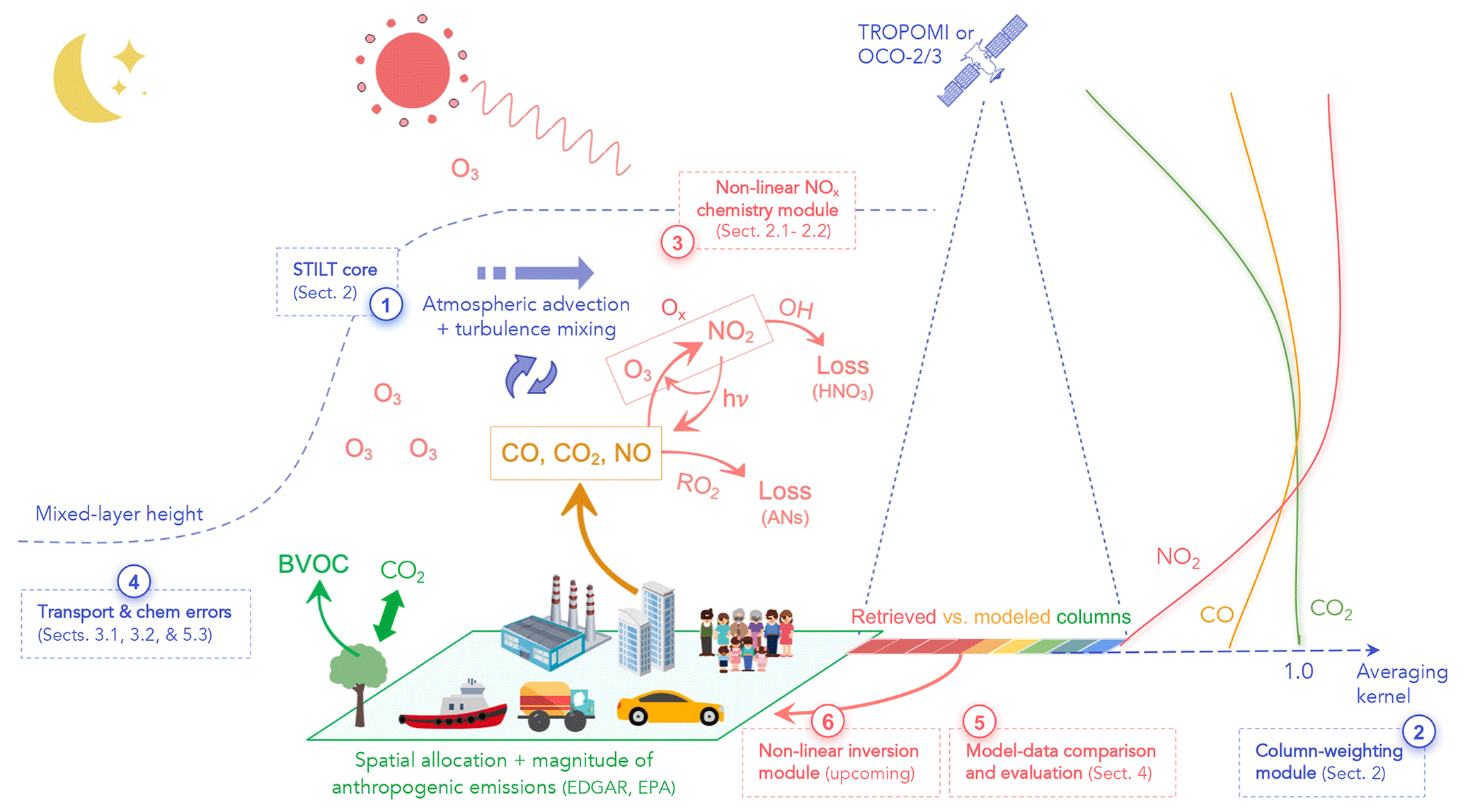
Figure 1 A conceptual diagram of our proposed local-scale multi-tracer modeling framework in interpreting column observations. It contains a road map for this study (points 1 through 5). The diagram highlights the key biogenic, physical, and/or chemical processes for quantifying NO_x, CO, and CO₂ around cities, based on space-based measurements (pixels from red to blue). These include details on the atmospheric conditions (wind speed and planetary boundary layer height for vertical mixing, horizontal mixing, and diffusion lengths); chemical conditions (photolysis rate and NO_x regimes and regional versus local oxidant conditions); the spatial distribution of emissions (urban vs. power plant); and sensitivities of the column abundance to individual vertical levels (averaging kernel).

Making full use of the existing and upcoming satellites that retrieve concentrations of APs and GHGs offers an informative way to target urban emissions from different sources at a policy-relevant scale of a few kilometers. Combining satellite observations of species with different atmospheric lifetimes has enabled studies to diagnose chemical conditions and meteorological processes (Jin et al., 2017; Lama et al., 2022), identify urban plumes, constrain emissions for the tracer of interest (Wunch et al., 2009; Yang et al., 2023), and obtain observation-based ratios between tracers (Silva and Arellano, 2017; Wu et al., 2022; MacDonald et al., 2022) to infer structural changes in combustion activities (Reuter et al., 2014; Miyazaki and Bowman, 2023). In light of the rapid rise in satellite data volume, it is beneficial to have an analysis system that adequately accounts for the important local-scale processes in interpreting the abundance of GHGs and APs in a coupled manner (Fig. 1). Analogies to such local-scale systems in a global context include the AP-focused Tropospheric Chemistry Reanalysis version 2 (TCR-2; Miyazaki et al., 2020) and the GHG-focused Carbon Monitoring System Flux (CMS-Flux; Hurtt et al., 2022). Only a few recent multi-tracer modeling systems aim to bridge CO₂ and NO₂ column measurements (Reuter et al., 2014; Kaminski et al., 2022; Hakkarainen et al., 2023), despite limits in their modeling tools (elaborated upon in the next paragraph). In addition, as emphasized in Reuter et al. (2014), most multi-tracer studies rely on emission ratio or conversion ratio from inventories, which can be problematic.

In efforts to interpret CO₂ or NO_x emission signatures from satellite observations, most prior studies used either statistical or inversion approaches. The former approach involves the use of a Gaussian plume or exponentially modified Gaussian distribution (EMG) models with input from simple wind information to derive emissions of CO₂ and NO_x (or a lifetime if for NO_x) purely from observations in a computationally efficient manner without relying much on prior assumptions of emissions (Nassar et al., 2022; Beirle et al., 2011). These statistical approaches only provide a plume-integrated emission estimate that can be sensitive to the input wind speed and chemical lifetime. Multiple satellite overpasses need to be aggregated with wind direction aligned for a robust fit in the EMG model to obtain the emission and lifetimes. It is challenging to infer and evaluate sub-grid-cell variations in emissions. The more sophisticated inverse approach involves the use of a chemical transport model (CTM) that comprehensively accounts for atmospheric transport and chemical transformation and a coupled inversion or data assimilation system (e.g., Liu et al., 2022; Qu et al., 2022). CTMs are, however, computationally expensive and often involve hundreds of species and their coupling reactions. Most CTMs used in AP-related studies are Eulerian models, which may suffer from complications caused by rigid model grids (Wohltmann and Rex, 2009; Valin et al., 2011). Motivated by these approaches that rely on a constant lifetime or solve for individual chemical reactions, we have built a modeling framework to balance the advantages and imperfections – i.e., to simplify the chemical transformation process that preserves the non-linear relationship between NO_x emissions and the observed concentration field, together with a high-resolution atmospheric transport using a Lagrangian particle dispersion model (LPDM).

LPDMs have been increasingly utilized for emission estimates over the past few decades. For instance, the Stochastic Time-Inverted Lagrangian Transport model (STILT; Lin et al., 2003) building upon HYSPLIT (Stein et al., 2015) has been well adapted to analyze emission signals from all sorts of measurement platforms. STILT was designed to better describe the movement of air parcels only relevant to an observation site and explicitly provide the source–receptor relationship (i.e., the Jacobian matrix) to facilitate efficient atmospheric inversions for optimizing emissions. Besides, LPDMs themselves possess inherent numerical and computational advantages, such as avoiding artificial smoothing of concentration fields by spurious numerical diffusion in confined model boxes (Wohltmann and Rex, 2009; Lin et al., 2013). More importantly, the Lagrangian transport perspective is intuitively coupled with box models that handle chemical reactions. Noticeable examples include STOCHEM (Collins et al., 1997), ATLAS (Wohltmann and Rex, 2009), CLaMS v2.0 (Konopka et al., 2019), and HYSPLIT-based variations, including HYSPLIT CheM (Stein et al., 2000), ELMO-2 for ozone (Strong et al., 2010), and STILT-Chem (Wen et al., 2012). These Lagrangian chemical models describe the chemical reactions of each species or lumped group with similar functional groups to calculate chemical transformation along trajectories but vary in the complexity of implemented chemistry and parameterization for turbulent mixing and numerical diffusion. Despite these prior modeling efforts, Lagrangian chemical models are more often adopted to inform the origins of APs but are less commonly used to constrain emissions. Such under-appreciation is in part a result of the heavy computational expenses in solving chemical changes at a high frequency via ordinary differential equations (similar to most Eulerian CTMs) and the reliance on external meteorological fields.

To reduce computational costs in dealing with complex chemistry, studies have proposed machine learning techniques or defaulted to a constant-lifetime assumption as a shortcut. Machine learning techniques have been applied to approximate the chemical mechanisms (Keller and Evans, 2019; Huang and Seinfeld, 2022), predict the OH field with observational constraint (Zhu et al., 2022), and calculate emissions (He et al., 2022). Other studies have assumed a constant first-order lifetime to estimate NO_x emissions and emission ratios between NO_x and CO₂ (Lee et al., 2014; Hakkarainen et al., 2023). However, unlike chemically passive species such as CO₂, the chemical tendency of NO_x is not independent of atmospheric advection and turbulent mixing because of the chemically driven non-linearity between the NO_x lifetime and the NO and NO₂ concentrations (Laughner and Cohen, 2019). More specifically, during the day, NO_x is lost through two more permanent pathways of (1) NO₂ + OH to nitric acid and (2) NO + peroxy radicals (RO₂), with a minor branch in producing alkyl nitrates or ANs (point 3 in Fig. 1). The two pathways compete with one another and either may dominate, depending on the chemical conditions. Such non-linear dependence of the NO_x lifetime or chemical tendency with the NO_x concentration must be accounted for to estimate the NO_x emissions from atmospheric NO₂ concentrations. Such non-linearity will affect the interpretation of tracer-to-tracer emission ratios from observed enhancement ratios.

In this study, we present a non-linear modeling framework, STILT–NO_x, to simulate tropospheric column-averaged NO₂ mixing ratio (tNO₂) as retrieved from the TROPOspheric Monitoring Instrument (TROPOMI). Note that initial NO₂ vertical column density (VCD; $\mathrm{molec}.{\mathrm{cm}}^{-\mathrm{2}}$) is converted to tNO₂ (ppb) by dividing by a dry air VCD. The dry air VCD is calculated by integrating a profile of the ideal gas number density of air minus a modeled water vapor profile. As illustrated in Fig. 1, the overarching goal of this framework is to facilitate emission optimizations over global anthropogenic hotspots by simulations of the concentrations of key trace gases of CO₂, CO, and NO_x at the local scale. To do so, the current work aims to equip the STILT model with simplified chemistry that avoids explicit calculations of chemical reactions, while preserving the non-linearity that ties the NO_x concentrations to its emission (point 3 in Fig. 1). The proposed STILT–NO_x framework is comprised of four components, outlined below, which correspond, respectively, to points 1 to 4 in Fig. 1 and will be coupled to an upcoming non-linear flux inversion module (point 6).

1. The HYSPLIT–STILT core resolves fine-scale atmospheric advection and turbulence and calculates the sensitivity of concentration anomalies to upwind fluxes (footprint) (Lin et al., 2003; Fasoli et al., 2018; Loughner et al., 2021), with an additional simplified inter-parcel mixing scheme (Sect. 2.3).

2. A column-weighting module to simulate atmospheric columns (and uncertainties) that incorporates pressure weighting functions and retrieval-specific averaging kernel profiles (X-STILT; Wu et al., 2018).

3. A simplified chemistry module that describes the NO_x chemical tendency (Sect. 2.1) and how much NO_x is presented as NO₂ (i.e., NO₂ : NO_x ratio; Sect. 2.2).

4. An error analysis module that quantifies errors and biases in wind fields and chemical parameters (Sect. 3), following the methods initially proposed in Lin and Gerbig (2005) and Wu et al. (2018), which can be used for future flux inversions.

We illustrate the skill of this framework using comparisons of modeled tNO₂ and those diagnosed from TROPOMI over three United States (US) power plants and two cities across seasons (Sect. 4). Last, we discuss possible future advances in Sect. 5.3 and demonstrate the benefits of applying this framework, especially on the quantification of CO₂ emissions, emission ratios between NO_x and CO₂, and near-field wind biases in Sects. 5.1 and 5.2.

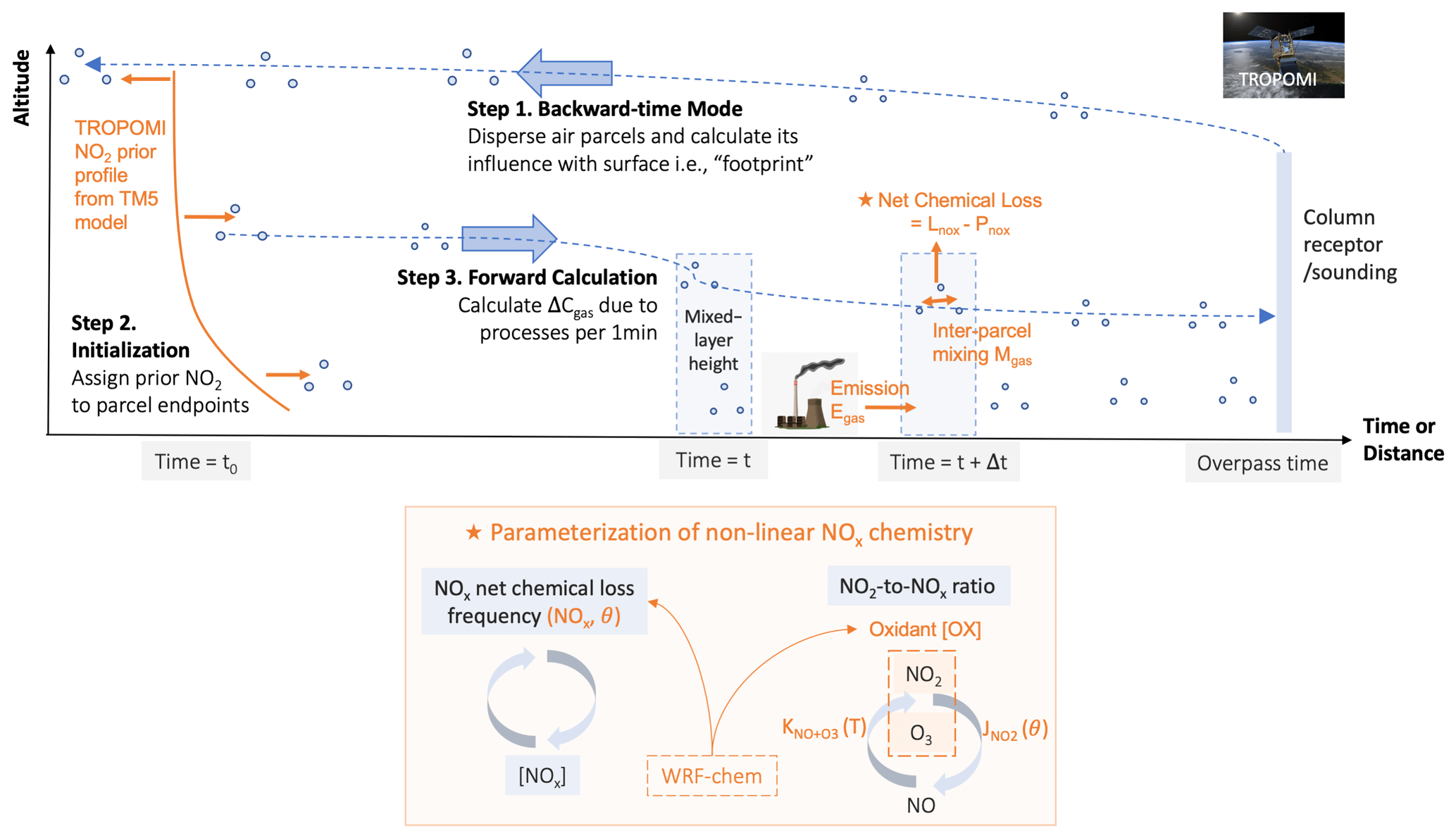
Figure 2 A schematic of STILT–NO_x for simulating concentrations in three steps. Step 1 is a routine backward-time calculation that records the locations of air parcels at each timestamp (Δt) of 1 min or shorter and their influence from potential fluxes (footprint). Step 2 is to calculate the initial condition for which the trajectory endpoint at time t₀ is given a concentration from 4D fields (e.g., TM5 in the case of NO_x). Step 3 is a forward-time concentration calculation that updates change in concentrations due to emissions, net chemical losses, and inter-parcel mixing along each trajectory at a timescale of ≤ 1 min. To clarify, Step 3 makes use of trajectories originating from a column receptor stretching from the surface to 2 km, as generated from Step 1.

2 STILT–NO_x model descriptions

Building upon the HYSPLIT–STILT atmospheric transport core, the STILT–NO_x framework traces the origin of the atmospheric column observed by the satellite and calculates changes in the NO_x concentrations due to emissions, inter-parcel mixing, and chemical transformations at the (sub-)minute scale. The STILT–NO_x simulations are conducted in three steps (Fig. 2).

First, the backward-trajectory mode records the latitude, longitude, and pressure coordinates of air parcels originating from the same atmospheric column sampled by satellites and being driven by the Eulerian meteorological fields (Step 1 in Fig. 2). In this work, we test two meteorological fields when they are available for each examined region, namely from the Global Forecast System (GFS0p25) and the High-Resolution Rapid Refresh (HRRR), with a respective horizontal grid spacing of 0.25^∘ and 3 km (Rolph et al., 2017). As most anthropogenic and all soil sources of NO_x are from the surface, air parcels are evenly distributed and released from the surface to 2 km, which is slightly above the typical planetary boundary layer (PBL) height (Wu et al., 2018). To evaluate how representative enhancements between 0 and 2 km are compared to the total tropospheric column enhancements (which can include sources from lightning and aviation), we analyzed vertical distributions of NO_x mixing ratios from TCR-2 (Miyazaki et al., 2020). TCR-2 is a global chemical reanalysis that includes full physical and chemical processes for various species and assimilates multiple satellite products of NO₂, ozone, CO, and SO₂. As a result, the monthly mean NO_x concentrations over the 2^∘ × 2^∘ area around the top 1000 cities is quite insignificant for pressure ≤ 700 hPa when compared to huge signals within the PBL (Fig. S1 in the Supplement). Although 0 to 2 km columns include most anthropogenic enhancements over urban areas, we subtracted a local NO₂ background from the total tropospheric columns to minimize the non-anthropogenic influences with a plume detection algorithm, following Kuhlmann et al. (2019). The model–data comparisons with background subtracted are discussed in Sect. 4.1.

After being released from a given TROPOMI sounding at the overpass time (∼ 13:00 local time for nadir soundings), air parcels are dispersed backward in time for 12 h (time at t₀ in Fig. 2). Step 1 also provides the STILT footprint ($\mathrm{ppm}(\mathrm{\mu }\mathrm{mol}{\mathrm{m}}^{-\mathrm{2}}{\mathrm{s}}^{-\mathrm{1}}{)}^{-\mathrm{1}}$) per air parcel per timestamp (Lin et al., 2003). The STILT footprint of a given air parcel is proportional to the time this parcel spends in a small area (of ∼ 100 m) and describes how the downwind concentration may be altered if this air parcel is influenced by emissions. A much more complete description of STILT can be found in Lin et al. (2003); Fasoli et al. (2018). The footprint concept, by definition, relies on atmospheric transport and only accounts for concentration changes due to emissions but not chemical transformations.

Next, NO_x concentrations at the endpoints of the model trajectory are extracted from the Tracer Model version 5, massively parallel version (TM5-MP) to serve as the initial conditions (Step 2 in Fig. 2). TM5-MP is an auxiliary dataset in which the NO₂ vertical profiles serve as the prior knowledge facilitating the stratosphere–troposphere separation in Level 2 (L2) NO₂ retrieval (Van Geffen et al., 2022). Here, we simply assume that most NO_x is presented as NO₂ at nighttime, despite the apparent caveat for neglecting NO₃ chemistry and heterogenous reactions involving N₂O₅.

Once NO_x is initialized at the time t₀ for the endpoint of every trajectory, we proceed with Step 3 (Fig. 2) to estimate the changes in concentrations due to emissions, chemical transformation, and inter-particle mixing. Mathematically, the concentration per air parcel per timestamp (C_p,t) relies on that from the last timestamp, following Eq. (1):

$$\begin{array}{}\text{(1)}& \begin{array}{rl}{C}_{\text{p,t}}=& C_{\text{p,t}-\mathrm{\Delta }t}+\mathrm{\Delta }{C}_{\text{emis,p,t}}(E,F_{\text{p,t}})\\ & +\mathrm{\Delta }{C}_{\text{chem,p,t}}(C_{\text{p,t}},{\mathit{\theta }}_{\text{p,t}})+\mathrm{\Delta }{C}_{\text{mix,p,t}}(C_{\text{p,t}},\stackrel{\mathrm{‾}}{C_{{\mathrm{p}}_{\text{ngb}},\mathrm{t}}}),\end{array}\end{array}$$

where the time interval for updating concentrations, Δt, is defaulted to 1 min or reduced to a sub-minute value when C_t becomes nonphysically negative to ensure numerical stability. Concentration gains from emissions, ΔC_emis, result from multiplying STILT-parcel-specific footprints (F_p,t) with prior emissions (E) from EDGARv6.1 (Monforti Ferrario et al., 2022) and the U.S. Environmental Protection Agency (EPA; United States Environmental Protection Agency, 2022) for power plant cases in this study. We neglect soil NO_x emissions, given the relatively small contributions in cities. Unlike sophisticated CTMs which resolve the chemical reactions of an individual or lumped groups of species, concentration anomalies due to chemical reactions, ΔC_chem, are solved in an explicit first-order fashion involving a net chemical tendency, with a unit of parts per billion per hour (ppb h⁻¹). Such a chemical tendency ($R_{{\mathrm{NO}}_x}$ in Eq. 2b) is parameterized offline as functions of NO_x concentrations and solar zenith angles, θ, which is explained in Sect. 2.1. The final term, ΔC_mix,p,t, denotes the concentration exchange between a given air parcel and its volumetric neighborhood (p_ngb), which is explained in Sect. 2.3.

Following these steps, we obtain the modeled NO_x mixing ratio for every trajectory released between the surface and 2 km, based on NO_x curves described in Sect. 2.1. To compare against TROPOMI tropospheric NO₂ columns, we account for the fraction of NO_x that is present as NO₂ (Sect. 2.2) and properly weight the modeled NO₂ from different altitudes, according to the pressure weighting function and averaging kernel profiles, following Wu et al. (2018). Such an approach in applying averaging kernel (Fig. 1) to the modeled profiles is equivalent to a more commonly used approach, which re-calculated the retrieved tNO₂, as seen from the CTM, by re-calculating the air mass fraction based on modeled NO_x profiles, as investigated in Goldberg et al. (2022). In addition, we evaluate the modeled meteorology and chemistry using a separate set of STILT–NO_x simulations with true NO_x emissions from the EPA for three US power plants (Sect. 4.1).

2.1 NO_x net chemical tendency, $R_{{\mathrm{NO}}_x}$, and uncertainty

Inspired by the theoretical non-linear curves of NO_x lifetimes as functions of NO₂ vertical column density and volatile organic compound reactivity (VOC_R) and based on a box model in Laughner and Cohen (2019), we extract similar non-linear parameterizations using the Weather Research and Forecasting model coupled with Chemistry (WRF-Chem v4.0.2; Grell et al., 2005). Focusing primarily on polluted environments, we carried out WRF-Chem simulations for three mid-latitude cities and extracted model outputs from a 2^∘ × 2^∘ region centered around each city. Three cities, namely Los Angeles in the USA, Shanghai in China, and Madrid in Spain, represent typical megacities in North America, Asia, and Europe. Their varied climatic conditions and sectoral emissions of NO_x, VOC, and GHGs provide a holistic view of the variability in the NO_x chemical tendency. While our analyses extended to power plants and cities beyond these three training sites when compared to TROPOMI data (Sect. 4), it helps assess the broader applicability of our chemical parameterizations.

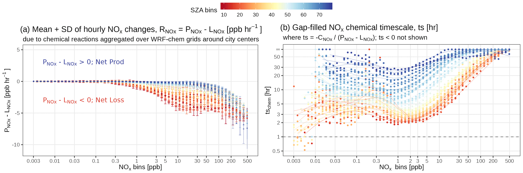
Figure 3 A diagram of NO_x net chemical loss tendency ($R_{{\mathrm{NO}}_x}$; ppb h⁻¹) as functions of the NO_x concentration ($C_{{\mathrm{NO}}_x}$) and solar zenith angle (θ). The net loss timescale was first calculated for each 12 km grid cell of all WRF-Chem simulations for three cities (with specific model setups summarized in Appendix A) and then aggregated into multiple bins of NO_x concentration (ppb). The NO_x bins are equally divided in the logarithmic space. The solid dots and error bars denote the average and standard deviation of $R_{{\mathrm{NO}}_x}$ within each combined θ and $C_{{\mathrm{NO}}_x}$ bin. For the net loss timescale, only positive values are displayed, given the logarithmic scale of the y axis in panel (b), and data points with values > 72 h are simply treated as infinite.

Appendix A describes our specific WRF-Chem settings used to generate lookup tables of NO_x chemical loss tendencies, which we will refer to as NO_x curves (Fig. 3). Of the WRF-Chem settings, the chosen chemical mechanism (Regional Acid Deposition Model or RADM2; Stockwell et al., 1990) is the most relevant to the accuracy of these NO_x curves. Despite uncertainties in these WRF-Chem simulations, what matters the most for reproducing the NO_x tendency is how NO_x varies with, for example, the solar zenith angle (SZA) and ozone, rather than the exact accuracy of NO_x concentrations themselves (from WRF-Chem). Thus, non-chemical components (prior emissions, boundary conditions, and physical processes) in this specific WRF-Chem configuration do not necessarily need to be perfect or optimized against observations. We clarify that WRF-Chem simulations had been performed to facilitate the parameterization of the NO_x tendency within STILT–NO_x but are not required when running STILT–NO_x.

By leveraging WRF-Chem's chemical diagnostic capability, we derive the net chemical tendency of NO_x within each hour ($R_{{\mathrm{NO}}_x}$, ppb h⁻¹) for every model grid within the lower 12 vertical levels ($x,y,z$). $R_{{\mathrm{NO}}_x}$ is calculated specifically from the cumulative changes in NO and NO₂ concentrations, solely due to chemical reactions (i.e., chem_no2 and chem_no in WRF-Chem registry), following Eq. (2):

$$\begin{array}{}\text{(2a)}& {\displaystyle }\begin{array}{rl}\sum _{h_{\mathrm{0}}}^h\mathrm{\Delta }{C}_{{\mathrm{NO}}_x}(x,y,z)=& \sum _{h_{\mathrm{0}}}^h\mathrm{\Delta }{C}_{\mathrm{NO}}(x,y,z)\\ & +\sum _{h_{\mathrm{0}}}^h\mathrm{\Delta }{C}_{{\mathrm{NO}}_{\mathrm{2}}}(x,y,z)\end{array}\text{(2b)}& {\displaystyle }\begin{array}{rl}& R_{{\mathrm{NO}}_x}(x,y,z,h)=P_{{\mathrm{NO}}_x}(x,y,z,h)-L_{{\mathrm{NO}}_x}(x,y,z,h)\\ & ={\displaystyle \frac{{\sum }_{h_{\mathrm{0}}}^h\mathrm{\Delta }{C}_{{\mathrm{NO}}_x}(x,y,z)-{\sum }_{h_{\mathrm{0}}}^{h-\mathrm{1}}\mathrm{\Delta }{C}_{{\mathrm{NO}}_x}(x,y,z)}{\mathrm{1}\mathrm{h}}},\end{array}\end{array}$$

where the model hour h denotes the start time of each hour interval in the WRF-Chem outputs, and z denotes the index of model vertical levels (i.e., from 1 to 12). ${\sum }_{h_{\mathrm{0}}}^h\mathrm{\Delta }{C}_{{\mathrm{NO}}_x}$ describes the cumulative net changes to the NO_x concentration, given the chemical reactions from the initial model hour h₀.

WRF-Chem pixel-specific hourly NO_x rate changes, $R_{{\mathrm{NO}}_x}$, are then grouped by both SZA (θ) bins, with a spacing of 2^∘, and $C_{{\mathrm{NO}}_x}$ bins, with equal spacing, in log10 scale (Fig. 3a). θ is chosen, given the close relation to solar radiation under clear-sky conditions, and controls the photolysis frequency of ozone and OH production (Rohrer and Berresheim, 2006) when the ozone and water vapor abundance remain unchanged. Because the intention in using STILT–NO_x is to inform the relationship between emission sources and satellite NO₂ columns, which are almost always filtered to remove cloudy scenes (i.e., quality assurance of ≥ 0.7), the choice of θ without considering cloud coverage is reasonable. Specifically, these net chemical changes explicitly contain all NO_x-relevant reactions within the WRF-Chem and RADM2 scheme, such as the recycling of NO_x from oxidized odd-nitrogen species like peroxyacetyl nitrate.

The above grouping procedure of $R_{{\mathrm{NO}}_x}$ is based on a finite number of bins of $C_{{\mathrm{NO}}_x}$, and θ unavoidably reduces the variability in the $R_{{\mathrm{NO}}_x}$ that were directly derived from WRF-Chem. To assess the extent to which the $R_{{\mathrm{NO}}_x}$ variability can be explained by the selected binning feature variables, we performed a sensitivity test to quantify the deviation of bin-averaged $R_{{\mathrm{NO}}_x}$ from the initial $R_{{\mathrm{NO}}_x}$. Generally, the $R_{{\mathrm{NO}}_x}$ variability is better preserved over polluted regimes with a higher-NO_x level > 1 ppb than over low-NO_x regimes (Fig. S2a and b in the Supplement). Choosing $C_{{\mathrm{NO}}_x}$ alone better explains the $R_{{\mathrm{NO}}_x}$ variability than choosing SZA or air temperature alone. Including additional variables (e.g., air temperature, NO₂ : NO_x ratio, and VOC_R) on top of our default choice of SZA and $C_{{\mathrm{NO}}_x}$ marginally improves the prediction of $R_{{\mathrm{NO}}_x}$, except for the inclusion of ozone. However, estimating ozone remains a challenging problem; thereby, ozone is not included as a feature variable in this study.

As a net result, $R_{{\mathrm{NO}}_x}$ is mostly negative during the day, meaning that NO_x is removed from the system. $R_{{\mathrm{NO}}_x}$ is large, with small spread at low θ of ≤ 20^∘ and gradually decreases during the day. $R_{{\mathrm{NO}}_x}$ becomes positive as it approaches the nighttime hours (Fig. S2c), and its variability peaks during sunset when $\mathit{\theta }\in [\mathrm{80}{}^{\circ },\mathrm{100}{}^{\circ }]$, with a fractional uncertainty of over 100 % (blue error bars in Fig. 3a) when considering the transition to nighttime chemistry. When focusing on the daytime portion with θ < 70^∘ and $C_{{\mathrm{NO}}_x}$ ≥ 1 ppb, the spread in $R_{{\mathrm{NO}}_x}$ among the WRF-Chem urban pixels ranges from 12.2 % to 67.9 %, according to varied θ and $C_{{\mathrm{NO}}_x}$ (red to yellow error bars in Fig. 3a), with an average uncertainty of 41.2 %. When focusing on the nighttime portion with θ ≥ 70^∘ and $C_{{\mathrm{NO}}_x}$ ≥ 1 ppb, the spread in $R_{{\mathrm{NO}}_x}$ spans from 27.9 % to over 100 %, with an average uncertainty of 96.3 % that is largely skewed by the high uncertainty around the dusk hours. Last, the average daytime uncertainty in the NO_x tendency at medium to high NO_x concentrations (i.e., 41.2 %) will be propagated into chemical uncertainties in tNO₂ for cases of power plants and urban areas, which is further described in Sect. 3.

Given the further fluctuation in $R_{{\mathrm{NO}}_x}$ with $C_{{\mathrm{NO}}_x}$, we define a net loss timescale (h) as ${\text{ts}}_{{\mathrm{NO}}_x}=-C_{{\mathrm{NO}}_x}/R_{{\mathrm{NO}}_x}$ and distinguish it from the conventional chemical lifetime that only accounts for chemical losses. For reference, a positive (or negative) timescale corresponds to a net loss (or production) of NO_x (Fig. 3b). The contribution from NO_x production is minor during noon hours. The non-linear dependence of ${\text{ts}}_{{\mathrm{NO}}_x}$ with $C_{{\mathrm{NO}}_x}$ is largely driven by several NO_x loss pathways (predominately by the loss processes of NO₂ +  OH and the formation of alkyl nitrates during the daytime and by the NO₃ chemistry and heterogeneous chemistry at nighttime; Fig. S2). Here, we do not differentiate between the NO_x curves by VOC_R, despite its critical role in determining the turning point when NO_x is mainly lost to either nitric acid or alkyl nitrates (Laughner and Cohen, 2019). We instead perform a sensitivity study of the impact on NO_x curves for three VOC_R intervals in Sect. 5.3. Note that these NO_x curves should be considered to be a first-order approximation and can certainly be improved upon to evaluate more complex parameterization (Sect. 5.3). When it comes to calculating chemical changes within STILT–NO_x per air parcel per timestamp (i.e., ΔC_chem,p,t in Eq. 1), such a loss timescale is looked up according to parcel-specific θ and $C_{{\mathrm{NO}}_x}$ to enable the non-linearity core (Fig. 2; bottom panel).

2.2 NO₂ : NO_x ratio

As only the vertical column density of NO₂ is retrieved, the fraction of NO_x present as NO₂ as TROPOMI passed over is an important component of our analysis. Prior studies estimated such ratios using a constant value (e.g., 0.75) at noon hours across seasons, with a 10 % uncertainty (Beirle et al., 2011, 2019; Goldberg et al., 2022), monthly mean climatology of ozone from reanalysis (Beirle et al., 2021), and CTMs. NO_x is primarily emitted as NO but converted to NO₂ via the reaction with ozone. During the daytime, NO₂ is photolyzed back to NO with a photolysis frequency, $J_{{\mathrm{NO}}_{\mathrm{2}}}$. Thus, the NO₂ : NO_x ratio scales with the ratio of ozone and $J_{{\mathrm{NO}}_{\mathrm{2}}}$ (Eq. 3a).

Considering the close coupling between NO₂ and O₃, their sum O_x in Eq. (3b) is a key indicator of the atmospheric oxidant capability for understanding the urban air chemistry (Clapp and Jenkin, 2001; Fujita et al., 2016) and informing chemical dynamics (e.g., during the COVID-19 pandemic; Parker et al., 2020; Lee et al., 2020). O_x levels within the PBL can be regarded as a NO_x-independent component related to regional ozone inflow plus a NO_x-dependent component that varies non-linearly with local NO_x and VOC_R conditions (Clapp and Jenkin, 2001; Jenkin, 2004). The complexity in the local O_x–NO_x non-linearity is caused by key reactions behind NO_x curves, which are discussed in Sect. 5.3.1.

For simplification, we prescribed a typical O_x level of 50 ppb in the first version of STILT–NO_x and calculated the NO₂ : NO_x ratio via Eq. (3), assuming a steady state.

$$\begin{array}{}\text{(3a)}& {\displaystyle }{J}_{{\mathrm{NO}}_{\mathrm{2}}}\left(\mathit{\theta }\right)\left[{\mathrm{NO}}_{\mathrm{2}}\right]& {\displaystyle }=k_{\mathrm{NO}+{\mathrm{O}}_{\mathrm{3}}}(T_{\mathrm{A}},P)\left[{\mathrm{O}}_{\mathrm{3}}\right]\left[\mathrm{NO}\right]\text{(3b)}& {\displaystyle }\left[{\mathrm{O}}_x\right]& {\displaystyle }=\left[{\mathrm{O}}_{\mathrm{3}}\right]+\left[{\mathrm{NO}}_{\mathrm{2}}\right],\end{array}$$

where $J_{{\mathrm{NO}}_{\mathrm{2}}}$ relies on θ for daytime, and the reaction rate coefficient of NO with O₃ ($k_{\mathrm{NO}+{\mathrm{O}}_{\mathrm{3}}}$) is a function of the air temperature T_A and pressure P (Fig. 2; bottom panel). The inclusion of O_x in calculating the NO₂ : NO_x ratio is to avoid a non-physical infinite conversion of NO to NO₂ at high-emitting sources, following the titration of the ambient ozone. Sensitivity tests were performed to reveal how biases in the prescribed O_x level may modify the modeled tNO₂ (Sect. 3). Typical NO₂ : NO_x ratios over the examined mid-latitude targets across seasons are summarized in Sect. 5.2. In the future, satellite observations of tropospheric ozone could be used to add the additional complexity of variable O_x.

2.3 Inter-parcel mixing

Eulerian chemical models often suffer from mixing or numerical diffusion that is too strong within their model grid, while Lagrangian models (equivalent to those possessing extremely high spatial resolution) may lack any mixing between air parcels that are normally assumed to be independent of one another (Lin et al., 2013; Brunner, 2012). Such a lack of mixing has a negligible impact on the passive tracers, as mixing alters only the spatial distribution of concentration among air parcels but not the resultant concentration averaged across parcels at the receptor. However, non-linear processes alter both the spatial distribution of parcel-specific concentrations and the average resultant concentration. As a result, the calculation of the total NO_x tendency will be sensitive to how inter-parcel mixing is parameterized. Common ways to realize turbulence mixing are through (1) stochastic processes followed by the exchanging or averaging properties of air parcels found within a certain mixing length (e.g., STILT-Chem; Wen et al., 2012), (2) implemented deformation-driven and instability-driven schemes that rely on atmospheric stability and wind shear or stress characteristics (e.g., CLaMS; McKenna et al., 2002; Konopka et al., 2019), and (3) diffusion approaches that require the vertical gradient of concentrations (e.g., CiTTyCAT and ELMO-2; Pugh et al., 2012; Strong et al., 2010).

Here we follow the STILT-Chem approach to enable a process of exchanging concentrations per timestamp among the air parcels in close proximity to each other (ΔC_mix term back in Eq. 1), which smooth the horizontal gradient of concentrations among those air parcels. Specifically, at the timestamp of t, the concentration for a given air parcel p is updated, based on the concentration gradient between p and its neighborhood according to a mixing timescale (τ_mix) within a grid volume, with a mixing length scale of a horizontal area and the mixed layer height for the height as follows:

$$\begin{array}{}\text{(4)}& C_{\text{p,t}}^{\prime }=C_{\text{p,t}}\exp \left(-{\displaystyle \frac{\mathrm{\Delta }t}{{\mathit{\tau }}_{\text{mix}}}}\right)+{\stackrel{\mathrm{‾}}{C}}_{{\mathrm{p}}_{\text{ngb}},\mathrm{t}}\left[\mathrm{1}-\exp \left(-{\displaystyle \frac{\mathrm{\Delta }t}{{\mathit{\tau }}_{\text{mix}}}}\right)\right],\end{array}$$

where $\exp (-{\displaystyle \frac{\mathrm{\Delta }t}{{\mathit{\tau }}_{\text{mix}}}})$ implies the degree of horizontal mixing, and $\stackrel{\mathrm{‾}}{C}\left(t\right)$ represents the average concentration among air parcels within the mixing volume. The update of $C_{\text{p,t}}^{\prime }$ from C_p,t responds to ΔC_mix in Eq. (1). A relatively fast mixing timescale of 3 h and a horizontal mixing length of 1 km is used for testing the mixing impact on modeling tNO₂. Although we neglect the mixing in the free troposphere and the mixing between the mixed layer and the free troposphere in this first model version, we tested a spectrum of the horizontal mixing scales and include possible future improvements (Sect. 5.3.2).

3 Model uncertainty in tNO₂ due to wind and chemistry

As atmospheric transport and chemical transformation are the two main components in any CTMs, we assess how uncertainties tied to the modeled wind field, NO_x loss timescale, and NO₂ : NO_x ratio may contribute to uncertainties in tNO₂ (in ppb).

$$\begin{array}{}\text{(5)}& {\mathit{\sigma }}_{\text{sim}}^{\mathrm{2}}={\mathit{\sigma }}_{\text{trans}}^{\mathrm{2}}+{\mathit{\sigma }}_{\text{ts}}^{\mathrm{2}}+{\mathit{\sigma }}_{\text{nn}}^{\mathrm{2}}.\end{array}$$

Here we briefly describe how various tNO₂ uncertainties were approximated, based on our understanding of errors in respective model parameters or inputs (i.e., wind error, NO_x chemical tendency, or O_x levels). To approximate the tNO₂ uncertainties due to transport errors, we followed previous approaches to first assess the GFS- and HRRR-modeled wind profiles against radiosonde; calculate respective error statistics including wind error, correlation time, and length scales; and, last, propagate wind error statistics into errors in column concentrations. Mathematically, ${\mathit{\sigma }}_{\text{trans}}^{\mathrm{2}}$ in Eq. (5) is derived from the difference in the variance of STILT–NO_x air-parcel-specific NO₂ concentrations between the original simulation and a second simulation with wind error (Lin and Gerbig, 2005; Wu et al., 2018). The derivations of modeled wind errors and contributions to tNO₂ errors are elaborated in Appendix B. To evaluate the impact due to errors associated with chemical parameters, we perturbed the NO_x curves or the O_x level according to 20 perturbing factors. Perturbed curves or parameters are used to generate 20 new sets of tNO₂ fields, of which their respective standard deviation among perturbations serves as the chemical uncertainty (ppb) due to NO_x net loss timescale and NO₂ : NO_x ratio (σ_ts and σ_nn in Eq. 5). These 20 perturbing factors were randomly selected from a normal distribution N ($\mathit{\mu }=\mathrm{1};{\mathit{\sigma }}_{\text{param}}$). Here we tested out σ_param of 40 % for NO_x loss timescales, according to uncertainties in the chemical tendency (Fig. 3) and a σ_param of 40 % for the O_x level (Eqs. 3).

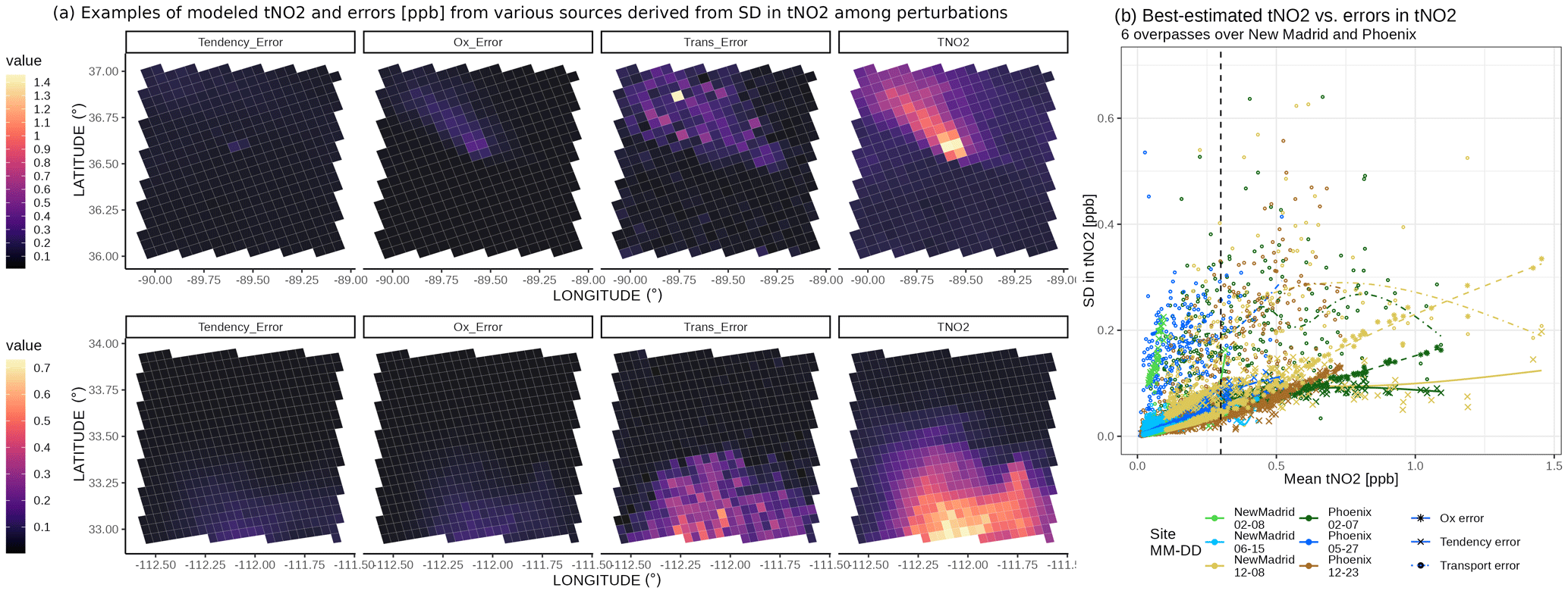
Figure 4 (a) Demonstrations of best-estimated tNO₂ (TNO2) and their uncertainties (ppb) due to random u or v wind errors (Trans_Error), NO_x chemical tendency (Tendency_Error), and O_x levels (Ox_Error) on 8 December 2020, over the New Madrid power plant (USA), and 23 December 2020, over Phoenix (USA). (b) Scaling between uncertainties and mean tNO₂ signals over six overpasses for the two targets with smooth splines fitted (crosses with solid lines for tendency errors, stars with dashed lines for O_x errors, and circles with dotted-dashed lines for transport errors). Colors differentiate the sites and TROPOMI overpass times.

Due to heavy computational expenses in conducting such wind and chemical perturbation analyses for all overpasses and locations, we only ran error analyses for a total of six overpasses over a power plant and a city. To cover the seasonal changes in the NO₂ signals and their uncertainties, overpasses in varied seasons are examined for the New Madrid (USA) power plant on 8 February, 15 June, and 8 December 2020 and Phoenix (USA) on 7 February, 27 May, and 23 December 2020. Two winter cases with relatively large signals are shown in Fig. 4a. Considering the non-linearity between the chemical tendency and NO_x concentration, sounding-specific uncertainties for all six cases are presented against modeled tNO₂ in Fig. 4b. When conducting those perturbations, other model parameters like the meteorological field and emissions remain unchanged.

As a result, the average percent error in u or v wind speed in the PBL is roughly 22 % for the New Madrid case (Fig. S3a in the Supplement), which contributes to 50 % uncertainty in tNO₂ at the sounding level (third column in Fig. 4a). Higher transport errors may occur more frequently if an intensive point source is in the area or over pixels on the border of the NO₂ plumes, with moderate signals of about 0.2 to 0.5 ppb (e.g., dots in Fig. 4b). This is because a small deviation in the modeled wind vectors causes air parcels to either hit or miss the intensive source. The transport uncertainty appears to first correlate positively with the signals and then decreases when signals are sufficiently high, e.g., > 0.7 ppb. Such a decline may be associated with hyper-near-field soundings, where the deviation in wind fields may not alter modeled signals, as modeled air parcels will always experience a large influence from the emission source (dotted–dashed lines in Fig. 4b). Compared to power plants, cities may be associated with a more homogeneous transport uncertainty if emissions are more homogeneous and better mixed in the PBL.

Given a roughly 40 % uncertainty in the O_x levels or NO_x chemical tendency, chemical uncertainties (in ppb) remain small when modeled signals are compared (Fig. 4a). Uncertainties from chemical tendency first increase with tNO₂ signals and gradually plateau for tNO₂ beyond 0.7 ppb, likely because NO_x is lost slowly when the NO_x concentration stays high, and further perturbations in the chemical tendency are less impactful. In contrast, the uncertainty from O_x levels appears to consistently scale against the signals, i.e., more apparent for soundings adjacent to the power plant, with reasons explained as follows. When the certain perturbed O_x level approaches zero, the amount of NO that can be oxidized as NO₂ becomes minimal (second column in Fig. 4a). This case mimics the scenario where O₃ can be titrated in proximity to an intense release of NO before the ozone-depleted plume air is mixed with the ambient ozone-rich air. Nevertheless, considering the entire sample, the percent of errors due to chemical parameters remains relatively low (13 % to 18 % for six cases in Fig. 4b).

Whether chemical or meteorological errors dominate the total model errors fundamentally depends on tropospheric NO₂ signals which further rely on factors like atmospheric stability with wind errors, chemical tendency, and emission distribution. Such a dependence leads to a spatial gradient and seasonal variations in estimated errors, as seen from the above examples. In brief, our limited perturbation experiments suggest that transport uncertainties dominate the total modeled uncertainties, except for a few hyper-near-field soundings, where chemical uncertainties become more substantial.

For future emission optimizations, uncertainties in the emissions, retrieval, and background should also be included. Despite the significant advance in the TROPOMI NO₂ retrieval version of v2 compared to v1 (Van Geffen et al., 2022), v2 retrieval is associated with a fractional uncertainty (normalized over retrieved tNO₂) of ∼ 30 % to 50 % for most soundings within the plume. Uncertainties in the NO_x emissions between inventories can serve as the prior uncertainty, which is substantial at the pixel level (Figs. S4 and S5 in the Supplement). Besides the regional wind assessment, a novel plume rotation algorithm based on model–data NO₂ plumes is proposed in Sect. 5.2 to quantify near-field wind biases.

4 Model–data evaluations and comparisons

The tropospheric NO₂ mixing ratio at a given sounding location is influenced by the regional inflow, atmospheric advection and turbulence mixing, underlying emission characteristics, and chemical changes en route to the sounding (Fig. 2). Modeled tropospheric NO₂ mixing ratios using a variety of model configurations are compared against retrieved values from TROPOMI. Such model–data comparisons help evaluate the overall model performance and the roles of individual physical and chemical processes with a naming convention of 〈MET〉_〈EMISS〉_〈GAS〉_〈PROC〉, which is explained as follows:

• 〈MET〉 represent the meteorological fields of either 0.25^∘ GFS or 3 km HRRR that are used to drive STILT air parcels.

• 〈EMISS〉 represent two prior NO_x emission inventories. EDGARv6.1 is presented with monthly mean emissions, and the latest year available (2018) is the primary one for simulating all cases. Hourly mean emissions from EPA reports are only used to evaluate modeled chemistry and meteorology for several US power plants (Sect. 4.1).

• 〈GAS〉 represent the simulated species, with a default string of TNO2 without subtracting a localized tNO₂ background. A separate comparison with the background subtracted is shown in multi-track comparisons (Fig. 6; Sect. 4.1).

• 〈PROC〉 denotes the physical and chemical processes considered per run. Two main configurations include (1) DEF runs, with both inter-parcel mixing and chemical parameterization included, and (2) NOCHEM runs, with mixing but without considering the NO_x chemical tendency. The NOCHEM runs do account for the NO₂ : NO_x conversion but as a constant ratio of 0.74, according to EMG-based studies.

Only model–data comparisons using TROPOMI v2 are shown. As the satellite averaging kernel (AK) and observed tNO₂ differ substantially between v1 and v2, modeled concentrations are weighted by the version-specific AKs to yield apples-to-apples comparisons. Changes in AKs and the retrieved and modeled values between versions are summarized in Fig. S6 in the Supplement.

4.1 Model validation: US power plants

The New Madrid power plant along the Mississippi River is a 1300 MW coal-fired power station (GEM, 2021), which ranks first in 2020 among the US power plants regarding NO_x emissions provided by EPA. The Thomas Hill and Martin Lake power plants ranked second and third in 2020, respectively. We also report results for an overpass over the Intermountain power plant in Utah, where the surrounding complex terrain is difficult to model properly. Let us start with two examples to illustrate plumes modeled by different model configurations (Sect. 4.1.1) and then present model–data comparisons over dozens of overpasses of the three power plants (Sect. 4.1.2).

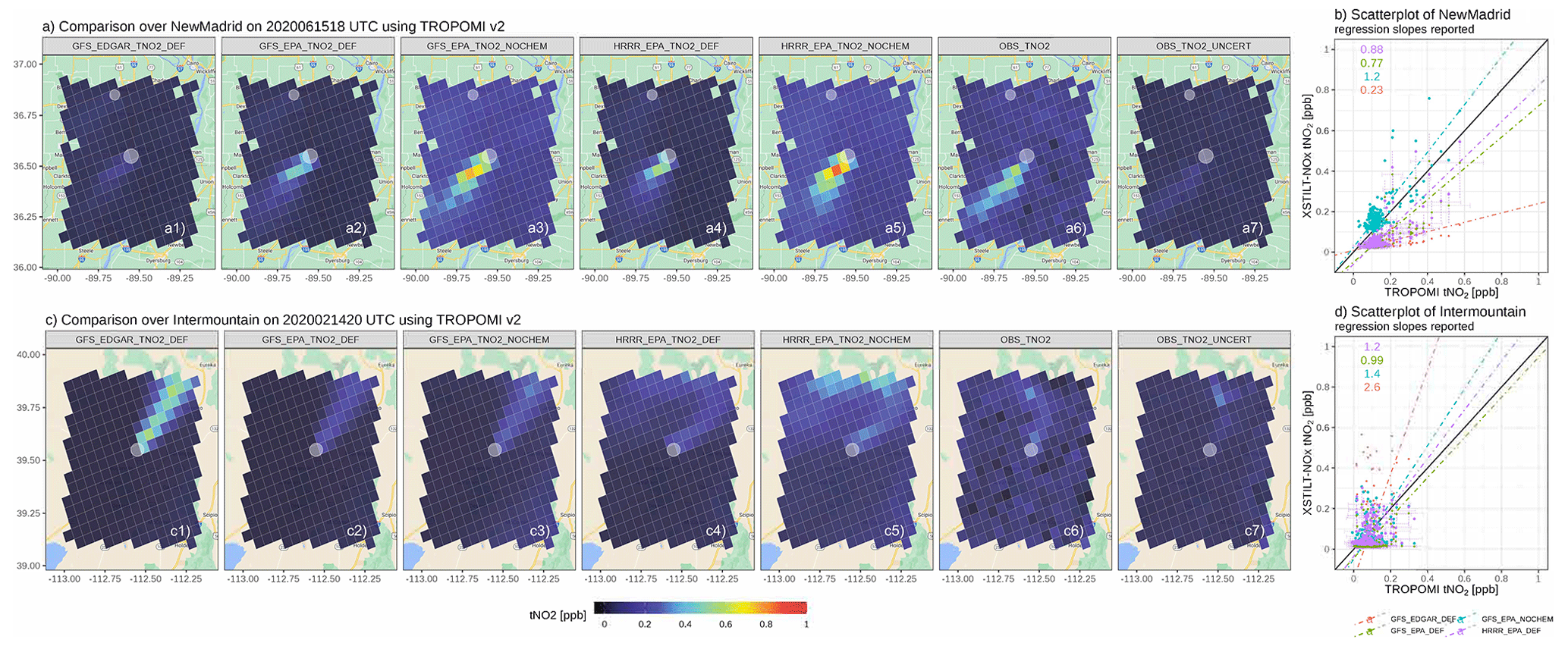
Figure 5 Maps (a) and scatterplots (b) of the modeled plumes, based on several model configurations (first five columns) versus retrieved plumes and uncertainties from TROPOMI v2.3 (last two columns) for the New Madrid power plant on 15 June 2020 and Intermountain, a Utah power plant, on 14 February 2020. Varied model configurations are labeled at the top of each panel, following the naming convention of 〈MET〉_〈EMISS〉_〈GAS〉_〈PROC〉, as explained in the list of Sect. 4. In particular, _DEF and _NOCHEM denote the modeled columns using the default (with mixing and chemistry) and non-chemistry configurations. Grid cells with intensive NO emissions from EDGARv6 are labeled as white circles, with the sizes denoting the relative emission magnitude. The type-II linear regression slope is fitted for each configuration (dotted–dashed line), and modeled and retrieval uncertainties are added (dashed error bars). The underlying road maps were created using the ggmap library in R (map data © 2023).

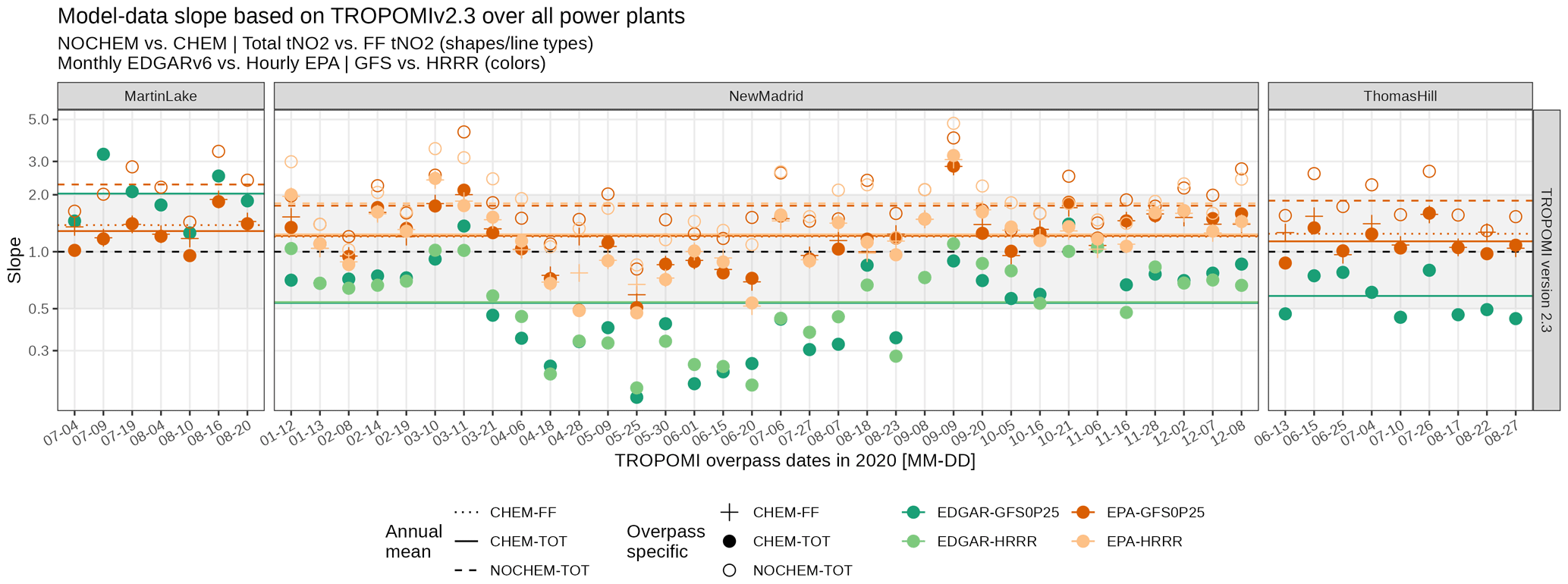
Figure 6 A summary figure of the linear slope between the observed tNO₂ and simulated tNO₂, using a variety of model configurations over all three US power plants. Model configurations include simulations (1) with or without NO_x chemistry parameterization (empty vs. solid dots); (2) using default EDGAR or scaled emissions from EPA (green vs. orange dots); (3) using 0.25^∘ GFS or 3 km HRRR (dark green or orange vs. light green or orange dots); and (4) using total tNO₂ or background-removed local enhancements (e.g., CHEM-FF as crosses). Annual mean slopes are displayed as horizontal solid or dashed lines. The model evaluation here uses TROPOMI v2.3 and emissions from EDGARv6.1. Evaluations that are based on TROPOMI v1.3 and annual mean EDGARv5 emissions are shown in Fig. S13a in the Supplement.

4.1.1 Single-track demonstration

The correction in NO_x emissions greatly improves the model–data alignment. For example, EDGAR-based simulations substantially underestimate or overestimate the tropospheric columns (Fig. 5a1 and c1), as EDGAR emissions are almost one-third or twice of the reported hourly EPA emissions for the New Madrid or Intermountain power plants, respectively (Fig. S7 in the Supplement). EPA-based simulations align better with retrieved values from TROPOMI v2, despite deviations over the far-field region (Fig. 5a2 vs. Fig. 5a6). Such improvements in the model–data alignment are also inferred from the linear regression slopes reported in Fig. 5b and d. Not accounting for NO_x chemistry or lifetime elevates NO₂ concentrations both within the plume and over the background, even if EPA emissions are assumed to be correct (Fig. 5a3 and a5). The inter-parcel mixing with a 3 h mixing timescale redistributes the NO_x concentrations among adjacent air parcels but leads to a minimal impact of ≤ 5 % of the modeled tNO₂ at individual column receptors (thereby not shown).

The choice of meteorological fields with different spatial resolutions insignificantly affects the modeled signals, except for cases surrounded by complex topography and flows. For example, the HRRR-based plumes resemble the GFS-based plumes for the New Madrid power plant (Fig. 5a2 vs. Fig. 5a4), which is also revealed by their similar wind error statistics (Fig. S3a). However, the complex terrain and stable PBL during wintertime complicate and usually worsen the model performance as a result of increased meteorological errors. On 14 February 2020, EPA-based plumes over the Intermountain power plant in Utah using two meteorological fields differ substantially from each other, and they both deviate from the observed plume regarding the plume shape. GFS delineates the mean wind direction within its coarser 0.25^∘ grid box, while 3 km HRRR offers more spatial variability in wind directions (Fig. 5c2 vs. Fig. 5c4). Yet, precisely capturing the curvature in the wind vector is extremely challenging, even when using 3 km meteorological fields (Fig. 5c6) and is more difficult when using Gaussian plume approaches that rely on only one effective wind vector. Such a model–data mismatch in plume shapes can further help to quantify the wind biases, which are discussed in Sect. 5.2.1.

Besides modeling challenges, the retrieval uncertainty cannot be neglected, as it ranges from 22 % to 31 % of the retrieved signal for the New Madrid case (Fig. 5a7) and up to 100 % for the Intermountain case (Fig. 5c7) at the sounding level. When using retrieved data and the averaging kernel from TROPOMI v1, the regression slope becomes 1.18 and 1.25 (Fig. S8 in the Supplement), indicating that modeled plumes using both meteorological fields are larger than observed plumes. While using TROPOMI v2, the respective slopes are 0.88 and 1.2 (Fig. 5b and d). This again emphasizes the substantial uncertainty in the retrieved signals, which is large enough to even alter the conclusion of whether emissions are underestimated or overestimated for a single overpass, and the need for analyzing multiple overpasses for evaluations (Sect. 4.1.2).

4.1.2 Multi-track evaluation

To provide a broad impression of the model performance, we expand the model–data comparisons to a total of 50 TROPOMI overpasses across all seasons in 2020, including 34 overpasses for the New Madrid power plant and 9 and 7 summertime overpasses for the Thomas Hill and Martin Lake power plants, respectively. These overpasses are selected based on their relatively intense signals compared to the surroundings. Model–data comparisons for all overpasses are shown in the maps in Figs. S9–S12 in the Supplement, with the linear regression slopes reported and summarized in Fig. 6 and Table S1 in the Supplement.

Cases with slopes deviating significantly from 1 are usually associated with substantial near-field wind directional biases. For instance, modeled wind vectors on 11 March, 28 April, and 9 September 2020 have directional biases of > 30^∘ (Figs. S9b and S10b), which explain the respective abnormal linear regression slopes of −1.75, 0.49, and 3.2 (Fig. 6). EDGAR-based simulations are biased too high or too low by a factor of 2 or more when compared to observed values from TROPOMI v2.3 (green dots in Fig. 6) that are driven by the biases in the EDGAR emissions (Fig. S7). The NOCHEM simulations without accounting for NO_x losses overestimate tNO₂ by a factor of 2 across all seasons and three power plants, regardless of the meteorological or emission fields adopted (empty circles in Fig. 6). Upgrading meteorological fields to a higher resolution seems to contribute less to the improvement of model–data agreements than correcting the emissions or chemistry. In the end, modeled values with NO_x chemistry and correct EPA emissions using either GFS or HRRR yield the best agreement with retrieved values from TROPOMI v2 (orange dots and lines in Fig. 6). When aggregating the results of all overpasses, simulations using the best knowledge of the emissions, the simplified chemistry, two different meteorological fields, and inter-parcel mixing are biased slightly high (regression slope up to 1.2; Table S1). RMSE values between the observed and modeled tNO₂ with NO_x chemistry-enabled range from 0.11 to 0.15 ppb (Table S1), which is comparable to the random uncertainty in the NO₂ retrieval of 0.09 ppb.

The statistics discussed above compared the total tropospheric NO₂ columns from the model and TROPOMI for soundings around each power plant. It is noticeable that modeled tNO₂ uncontaminated by emissions (i.e., background tNO₂) are sometimes slightly lower than observed background tNO₂ (Figs. S9a and S10a), possibly because higher chemical uncertainties are related to low-NO_x regimes, and non-anthropogenic NO_x sources from soil and lightning are excluded from current simulations but can play a significant role on tNO₂ over rural regions (Goldberg et al., 2022; Shah et al., 2023). In particular, column contributions from lightning NO_x emissions aloft may be amplified, since the TROPOMI NO₂ retrieval has a higher sensitivity towards the free troposphere than PBL. Since our current model setup only accounts for anthropogenic NO_x sources below 2 km, we conducted an additional test by subtracting the background tNO₂ from total tNO₂ to arrive at observed anthropogenic enhancements (the second paragraph in Sect. 2), assuming that the soundings within or outside the plumes have equal contributions from the nearby non-anthropogenic NO_x sources. After subtracting the tNO₂ background, the model–data comparison based on observed tNO₂ enhancements does not change dramatically (e.g., orange crosses vs. orange solid dots in Fig. 6).

In summary, using more accurate NO_x emissions with chemistry considerably improves the model–data comparison. Increasing the spatial resolution of meteorological fields has less impact on cases with relatively flat terrain. Larger model–data mismatches generally are associated with larger wind directional biases. Modeled values in tNO₂ may be biased to be slightly low in summer months from April to June and high in winter months from November to February, with minimal annual biases, assuming that the EPA emissions and observed tNO₂ are unbiased.

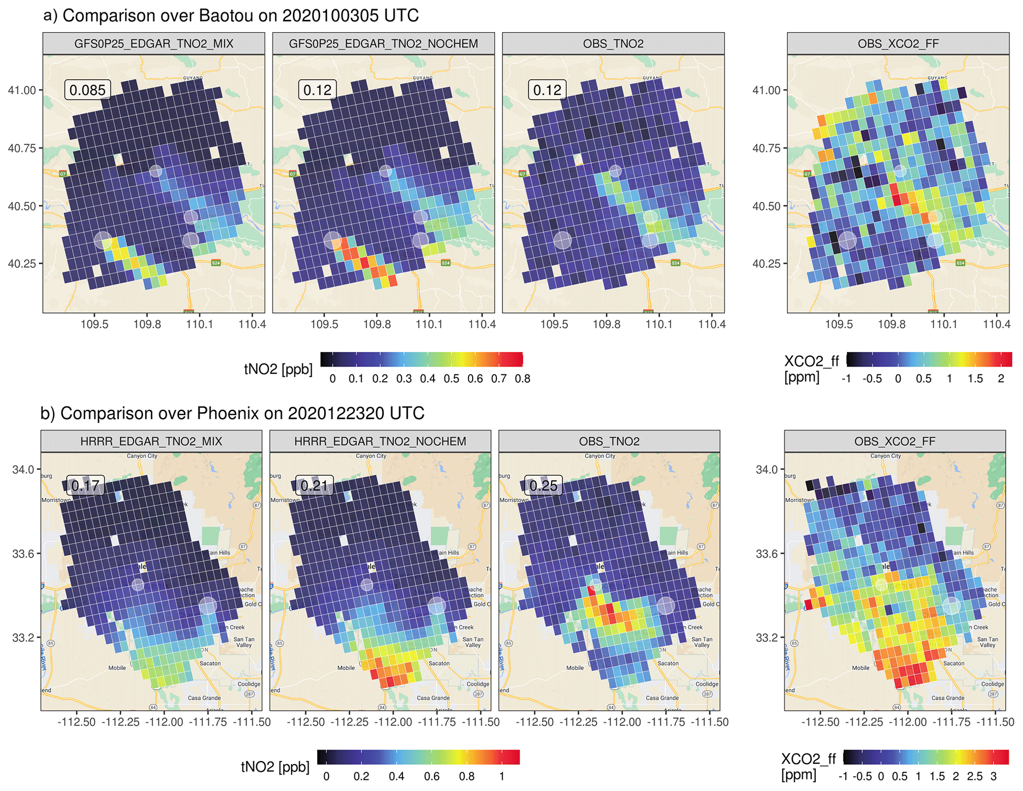
Figure 7 An example of GFS-based tNO₂ plumes over Baotou (China) on 3 October 2020 (a) and the HRRR-based tNO₂ plumes over Phoenix (USA) on 23 December 2020 (b). Modeled plumes are generated using annual mean ENO_x from EDGAR, with the top emitters highlighted in light-gray circles. Both observed tNO₂ and the anthropogenic XCO₂ enhancements from OCO-3 are plotted. XCO₂ enhancements calculated from a local background have been averaged based on the TROPOMI sounding size. Overpass time differences between TROPOMI and OCO-3 for the two cases are < 1 h. TROPOMI observations are cropped to match the boundary of the available OCO-3 soundings. The underlying road maps over Baotou and Phoenix were created using the ggmap library in R (map data © 2023).

4.2 Model application: two cities

We now move to city cases that include an industrial Chinese city, Baotou, and one of the fastest growing megacities in the US, Phoenix. As CO₂ and NO_x are commonly co-emitted into the atmosphere, observed XCO₂ enhancements derived from the Orbiting Carbon Observatory 3 (OCO-3) Snapshot Area Mapping (SAM) mode are displayed with observed tNO₂ (Fig. 7). Background XCO₂ is defined as the mean values over the background region that is determined by NO₂ plumes (modified from the background approach in Wu et al., 2018). Both cities possess relatively richer OCO-3 SAM observations co-located with TROPOMI data. Since no true NO_x emissions are available for cities, EDGAR is utilized as the prior emission inventory for simulating tNO₂ and optimizing NO_x emissions.

We simulated 18 and 12 TROPOMI overpasses, respectively, for Baotou and Phoenix (Figs. S14 and S15 in the Supplement) and first presented one example per city in Fig. 7. Baotou is surrounded by four point sources, as suggested by EDGARv6, but one large source in the city center, as informed by both the observed tNO₂ and XCO₂ enhancements on 3 October 2020 (Fig. 7a). Such a mismatch is confirmed by the comparison of normalized tNO₂ across all 18 TROPOMI overpasses with various wind speeds and directions (Fig. S14b), suggesting that EDGAR very likely misallocated anthropogenic NO_x sources. Similarly, the largest emission source to the east of the city center of Phoenix, according to EDGAR, seems suspicious and may again be misplaced when more overpasses are simulated (Fig. S15b). The observed plume is concentrated near the city center, compared to the HRRR-derived plume that dispersed farther away from the city center on 23 December 2020 (Fig. 7b). Such a spatial offset of the tNO₂ plumes is likely due to an overestimation in the modeled wind speed, which pushes the plumes to the southern edge while diluting tNO₂ values over the urban core.

When more overpasses are examined, the model captures the seasonal variation in tNO₂ well (i.e., higher or lower values in winter or summer months; Figs. S14a and S15a). Other than emission biases that affect all cases, a few overpasses stand out for Baotou, with poorer agreements with TROPOMI likely owing to (1) clear biases in wind direction on 31 May, 9 August, 15 December 2020, and 19 February 2021; (2) a likely overestimation in STILT footprint that may trigger several effects on 29 September, 29 March 2020, and 16 October 2021 (Fig. S14a). Although STILT can characterize the sub-grid-cell turbulent mixing by its stochastic nature, the 0.25^∘ GFS may be insufficient to resolve the complex terrain and air flows, contributing to biases in wind directions and planetary boundary layer heights (PBLHs) over mountainous locations (Lin et al., 2017) such as over Baotou. Deviations in the PBLH may cause a cascade of effects, such as deciding up to what height the emissions are diluted, whether such height is above or below the emission or plume height, and chemical changes along the way. Such effects may be magnified under low-mixing and low-wind conditions where the model particularly struggles with the accuracy of PBLH. Without much mixing between the plume and background air, the prescribed available O_x level may be overestimated adjacent to intensive NO_x sources. Overestimation in the NO₂ concentration may further be amplified when considering the dependence of NO_x rate changes on its concentration. Hence, concentrations of chemically reactive species under low-mixing scenarios are extremely challenging to model properly with an extreme during the nighttime.

5 Discussion

Our ultimate goal is to explore what can be learned about the emission characteristics from anthropogenic hotspots with the joint use of space-based NO₂, CO, and CO₂ plumes. As an intermediate step, this study is informed by previous efforts to extract and constrain urban CO₂ emissions from satellites using a Lagrangian framework (Wu et al., 2018; Roten et al., 2022) and extends it to the interpretation of tropospheric NO₂ satellite data. To diagnose NO_x emissions from NO₂ column signals, we need to effectively account for how NO_x evolves in air parcels from its initial source to locations sampled by TROPOMI, making the Lagrangian perspective an ideal candidate. Now we discuss when and how such a framework can be of most use and also the possible future improvements.

5.1 Model advantages and flexibility

Our framework accounts for atmospheric transport and chemical transformation in a more rigorous way than typical statistical approaches such as the EMG method and in a more efficient way than full-chemistry models that explicitly resolve individual chemical reactions.

Another advantage of the STILT–NO_x design is that each of the three main components (trajectory calculations representing air transport, chemical production or loss of the target species, and optimization of emission) are independent and each can reuse the previously saved output from the others. For example, if one wanted to test how sensitive model concentrations were to the chosen chemical scheme, then the simulations of atmospheric transport can be reused via the storage of trajectory-based modeling, thereby reducing the computational cost. Our prototype demonstrates a global solution of the NO_x chemical tendency parameterized by the one set of NO_x curves in Fig. 3. Although this simplification may be thought of as a limitation, one can easily replace those default curves with alternatives that are tailored toward a specific region or regime of interest. Such flexibility can inform us of the influence on modeled columns from NO_x curves derived from different chemical mechanisms. Similarly, one can investigate the sole meteorological influence by diversifying the meteorological and mixing parameters. Moreover, because air parcels in LPDMs are not tied to a certain atmospheric tracer, we can estimate the concentrations of various species along model trajectories. It allows us to constrain emissions for multiple atmospheric constituents in a consistent framework, which may shed light on tracer–tracer analyses (Sect. 5.2).

The Lagrangian modeling approach has its inherent benefits. First, the generation and recording of trajectories can easily reveal the source regions that are only relevant to a specific satellite sounding and the sub-city-scale variations in emission characteristics (Wu et al., 2022). In addition to storing latitudinal and longitudinal coordinates and extrapolated meteorological quantities along every trajectory at each timestamp, STILT–NO_x outputs and records NO_x concentration changes due to every process, including emission, net chemical changes, and inter-parcel mixing at minute scales. Those trajectory-level concentration changes are further driven by several model configurations listed in Sect. 4, which facilitates model debugging and comprehends modeled results. See Sect. 5.2 for one of the applications. Second, the spatial resolution of concentration calculations is not bounded by the rigid boundary of model grid cells, which is particularly important for dealing with non-linear processes for chemically active species. As demonstrated in several studies (e.g., Valin et al., 2011), the grid-averaged concentration may undergo excessive mixing in Eulerian models, and the concentration-driven chemical tendency varies with the adopted spatial resolution. While the Lagrangian perspective solves for concentration changes at extremely high spatiotemporal resolutions, inter-parcel mixing schemes can be implemented to smooth the concentration gradients, whereas it may be challenging to recover the sub-grid-cell concentration gradients in the Eulerian framework unless also increasing the spatial resolution.

More broadly, the proposed simplified parameterization of the non-linear NO_x tendency or NO_x curves is not limited to the STILT framework and can potentially be incorporated into other Lagrangian modeling frameworks or even Eulerian frameworks with a fine spatial resolution to resolve the local variability in chemistry.

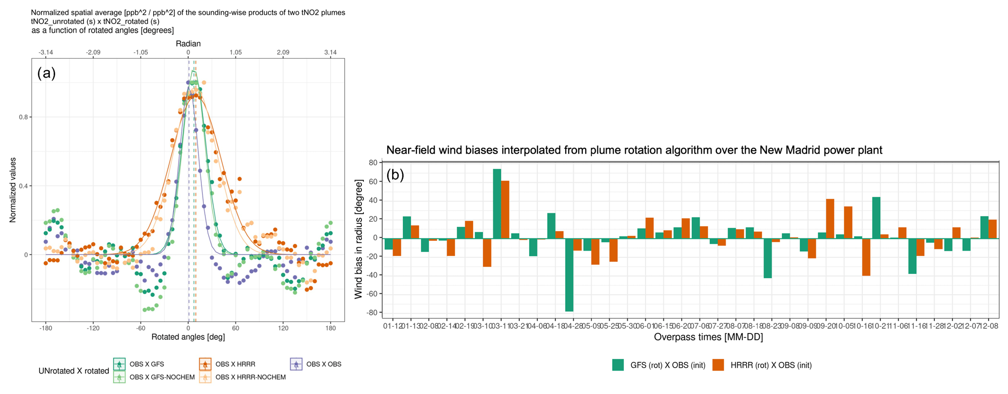
Figure 8 (a) An example of the normalized spatial mean of the sounding-wise product (ppb² ppb⁻²) between an unrotated observed tNO₂ and a rotated plume for the New Madrid power plant on 15 June 2020. Gaussian-like curves are fitted to each set, with the mean and standard deviation indicating modeled wind biases. Five sets of rotated plumes include observed tNO₂ (purple) and simulated tNO₂ driven by GFS (dark green) or HRRR (dark orange), with or without the account of the NO_x lifetime (light green or light orange). The horizontal dashed lines denote the μ parameter that can translate into wind bias in degrees or radians. (b) Near-field wind directional bias quantified by the modeled tNO₂ plumes, using 3 km HRRR (orange bars) or 0.25^∘ GFS (green bars), and retrieved tNO₂ plumes for every examined TROPOMI overpass (y axis; in degrees), following the rotation algorithm in panel (a).

5.2 Implications for constraining urban CO₂ emission and emission ratios

The knowledge learned from analyzing NO₂ plumes can be transferrable to constraining bottom-up CO₂ emissions. Two main sources of biases influencing the urban CO₂ emission constraint include biases in wind direction and emission locations. Model–data mismatches in NO₂ columns have shown great value in easily identifying the biases with emission locations, even without deploying atmospheric inverse analyses (Sect. 4.2), especially for point sources in urban areas, when plumes from multiple sources overlap less with one another. Additionally, diagnosing the NO_x emissions can facilitate CO₂ emission estimates in two ways. It can reveal systematic biases in near-field wind directions (Sect. 5.2.1) and quantify the NO_x : CO₂ emission ratios for point and/or area sources to assist in sector-based attribution (Sect. 5.2.2).

5.2.1 Quantifying wind bias

In addition to leveraging limited radiosonde measurements, the obtained modeled and retrieved NO₂ plumes can be used to quantify wind biases to improve the accuracy of top-down CO₂ emission constraints, whether or not conventional atmospheric inversions are employed. To do so, we conducted a second wind assessment involving a plume rotation algorithm. In brief, a NO₂ plume from either model or retrieval is rotated clockwise (α from −180 to −5^∘, with a spacing of 5^∘) or counter-clockwise (from 5 to 180^∘) around the emission source and then resampled onto the original TROPOMI pixels (Fig. S16 in the Supplement). tNO₂ from an original and a rotated plume are multiplied to arrive at a cross-product of tNO₂ (in ppb²), which is analogous to the concept of cross-correlation. The original or rotated plume can be chosen from either the model or observations, and their normalized cross-product can be expressed as a function of rotating angles (colors in Fig. 8a). More details on intermediate steps to calculate such a function are described in Appendix C.

As a result, the width of the Gaussian-shaped curve of the cross-product (as measured by the σ parameter of a Gaussian fit) reflects the bias in the plume shape resulting from horizontal dispersion. A larger area under the Gaussian curve indicates a greater overlap between the initial plume and the rotated plume. More importantly, deviations in the central line of the Gaussian fit away from zero (as measured by the μ parameter) imply possible biases in the near-field wind direction for each TROPOMI overpass (Fig. 8b). Specifically, wind directional biases of both GFS and HRRR appear to be smaller from May to early September than in the remaining months (Fig. 8b). A few outliers stand out due to large wind biases on 11 March, 28 April, 20 September, 5 October, 16 October, and 16 November 2020.

By identifying those outliers with strong wind directional biases, one can consider either removing those cases or assigning a larger observational uncertainty when attempting to constrain emissions of NO_x, CO, and CO₂, assuming that their emissions are mostly co-located. Alternatively, we can use this rotating algorithm to create a model plume with minimized wind directional bias before being fed into atmospheric inversions or data assimilation systems (which usually deal with random uncertainties). A more sophisticated approach would be to optimize the emission and wind field simultaneously (Liu et al., 2017). More investigations may be needed to examine the degree of freedom of such a wind-emission optimization framework.

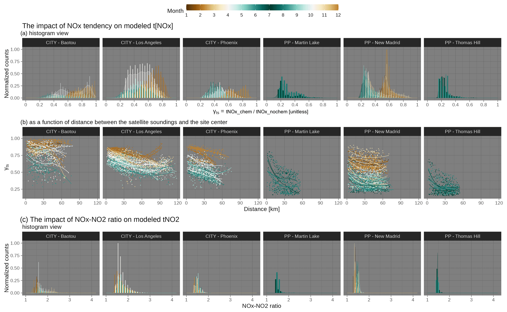
Figure 9 A quantitative metric of the impact from NO_x chemistry on tropospheric NO_x and NO₂ columns. Ratios in tNO_x between simulations with and without chemistry are calculated as ${\mathit{\gamma }}_{\text{ts,s}}={\mathrm{tNO}}_{x,\mathrm{CHEM},\mathrm{s}}/{\mathrm{tNO}}_{x,\mathrm{NOCHEM},\mathrm{s}}$, which is displayed as a histogram (a) and as a function of the distance of the satellite sounding from the site center (b). Soundings in summertime overpasses are colored in dark green, whereas brown is used for soundings in the dormant months. Soundings of all overpasses for all city and power plant cases are included in histograms. Only downwind soundings in the NO₂ plumes are included in the distance panel (b), with a smooth spline fitted per overpass to reveal the anti-correlation. The ratio between the modeled tropospheric NO_x column versus the tropospheric NO₂ column is derived from each sounding to reveal the NO₂ : NO_x ratio influence (c). As a reference, most previous studies adopted a constant NO_x : NO₂ ratio (reciprocal of NO₂ : NO_x ratio) of 1.32 and can reach 2 in a hyper-near-field area of a major NO_x source.

5.2.2 Quantifying emission ratios between NO_x and GHGs

Our modeling development offers additional insights into the discrepancy between emission ratios at the sources and directly observed enhancement ratios between two species with different chemical lifetimes. The joint use of NO₂ and CO₂ has enabled the calculation of emission ratios by adopting a spatial constant NO_x lifetime (MacDonald et al., 2022; Hakkarainen et al., 2023) and the constraint of CO₂ emissions using NO₂ plumes by adopting inventory-based emission ratios (Zheng et al., 2020; Zhang et al., 2023). However, inventory-based emission ratios might not be well constrained, and the impact of how NO_x decays over time and space on observed ENO_x : ECO₂ emission ratios has not been comprehensively assessed, which may impair the ability to accurately quantify such observed emission ratios (Kuhlmann et al., 2021).

Thanks to the ability of our model to track NO_x and NO₂ concentrations along trajectories with different model configurations, we can provide an assessment of the influence of atmospheric chemistry on estimating emission ratios. Specifically, the impact from NO_x net losses from each satellite sounding(s) is specified as the ratio of modeled tropospheric NO_x with chemistry over that without chemistry in the following: ${\mathit{\gamma }}_{\text{ts,s}}={\mathrm{NO}}_{x,\text{CHEM,s}}/{\mathrm{NO}}_{x,\text{NOCHEM,s}}$. Because NO_x is simply treated as a passive tracer like CO₂ in the NOCHEM simulations, γ_ts are naturally smaller than 1. Lower γ_ts corresponds to faster NO_x chemical frequency and more chemical losses en route to the sounding location, suggesting that NO₂ : CO₂ enhancement ratios derived directly from satellites need to be scaled up to render the ENO_x : ECO₂ emission ratios at source locations.

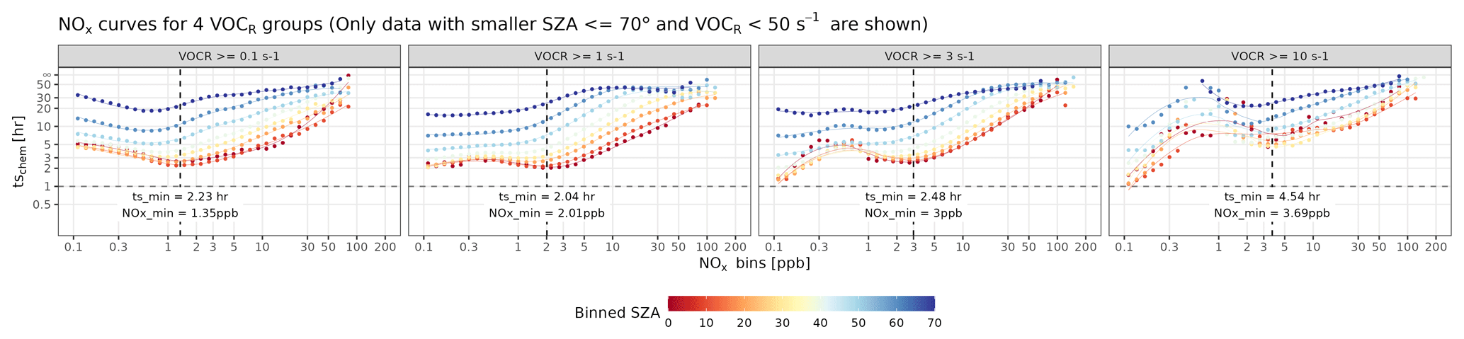
Figure 10 (a) Similar to Fig. 3b but differentiated by four intervals of VOC_R and SZA bins smaller than 70^∘, with a spacing of 10^∘. All panels here utilized model results from the same WRF-Chem simulations described in Sect. 2 and Appendix A.

We calculated γ_ts for every sounding and present their distribution as histograms in Fig. 9a or as a function of the distance from the emission source (Fig. 9b). γ_ts ranges from 0.24 to 0.61 for three power plants and from 0.42 to 0.84 for three cities, where lower values correspond to summer months (green bars in Fig. 9a). That is to say, the directly observed NO₂ : CO₂ enhancement ratios may have to be scaled up by 1.2 to even 4 times across seasons to properly recover the NO_x being lost en route from emission sources to the sounding locations. Not properly accounting for such an effect leads to an underestimation of the derived emission ratios from satellites. More importantly, discrepancies between enhancement ratios and emission ratios, reflected by γ_ts, are not spatially uniform. γ_ts gradually decline as soundings move away from the emission sources (Fig. 9b). Soundings located farther downwind of emission sources tend to undergo more chemical transformations, likely because NO_x losses become more rapid as NO_x concentrations become lower by atmospheric dispersion (triggering positive feedback). We clarify that only downwind soundings affected by major NO_x emissions are included in Fig. 9b, and simulations with or without chemistry have included the effect of atmospheric dispersion as distance increases. Furthermore, how quickly γ_ts declines with distance depends on the wind speed and heterogeneity in emissions. For example, the faster the wind may be, or the more isolated emissions there are, the steeper γ_ts decline with distance. γ_ts at the distance of 0 are much lower than 1 in summer, which suggests that the chemical transformation can affect the NO_x inflow. We further observe slight differences in the distribution of γ_ts for cities versus power plants. Histograms of both tropospheric NO_x (Fig. S17 in the Supplement) and γ_ts over cities are associated with a wider spread than power plants because cities contain a wider spectrum of emission types and intensities.

Last, enhancement ratios need to be adjusted considering the NO₂ : NO_x ratio and differences in averaging kernels among two retrievals. The medians of our estimated NO_x : NO₂ ratio over power plants and cities range from 1.33 to 1.66, which generally aligns with previous studies of around 1.32 (Beirle et al., 2011; Goldberg et al., 2022). Our estimates are lower in winter than in summer and can be as large as 2 or 3 for a few soundings experiencing intense NO_x sources (Fig. 9c).

5.3 Limitations and room for improvement

The diversity of VOC emissions, the vertical profiles of emissions, and the extent of inter-parcel mixing may impact the modeled results. Perhaps one of the biggest limitations of the current NO_x chemical representation lies in not directly accounting for VOCs, which may affect (a) the sweet spot on NO_x curves, where two NO_x loss pathways reach their maximum, and (b) the O_x-based NO₂ : NO_x ratios (Sect. 5.3.1). Moreover, the influence of representations of the emission profile on modeled tNO₂ can be magnified when further when considering the TROPOMI NO₂ averaging kernel (Sect. 5.3.2). Simulations of point sources like power plants may be more sensitive to these factors compared to simulations of areal sources.

5.3.1 The impact from VOC_R

To investigate the impact of VOCs on NO_x curves, we calculated the VOC reactivity against OH from existing WRF-Chem results, based on the following formula: VOC_R = $\sum i={\mathrm{1}}^n{k}_{\mathrm{OH}+{\mathrm{VOC}}_i}\left[{\mathrm{VOC}}_i\right]$ and generated separate sets of NO_x curves for four respective VOC_R intervals of [0.1, 1), [1, 3), [3, 10), and [10, 50) s⁻¹, with a coarse SZA bin spacing of 10^∘. Curves become much noisier at night and in pristine environments with extremely low NO_x (≤ 0.1 ppb), where WRF-Chem and RADM2 may be less suitable (thereby not shown in Fig. 10).

When considering lower SZAs (consistent with the TROPOMI overpass time of 13:00 local time), the general non-linear characteristic of these NO_x curves holds as VOC_R increases (Fig. 10). Higher VOC_R relative to lower NO_x concentration favors the oxidation of VOCs by OH and the associated minor loss pathway of NO + RO₂ to form alkyl nitrates with a minor branching ratio over the competing major NO_x loss pathway of NO₂ + OH (Fig. 1). With rising VOC_R, the NO_x chemical tendency becomes more positive (P – L; Fig. S18a in the Supplement), and the net loss timescale elongates (e.g., ts_min from 2 to 4 h in Fig. 10). Moreover, NO_x is required to reach a higher level to compete with the reactions involving VOCs, evident by the shift in the trough of the NO_x curves (e.g., NOx_min from 1.4 to 3.7 ppb in Fig. 10). To put it in context, the NO_x curves shown in Fig. 3 represent typical patterns, as long as VOC_R remains below 10 s⁻¹.

VOC_R may also affect the O_x level and the NO₂ : NO_x ratio. The prescribed O_x level of 50 ppb (Sect. 2.2) overlooks the non-linear O_x variability related to VOC_R (Murphy et al., 2007; Li et al., 2022). In NO_x-limited scenarios, OH favors the oxidation of VOCs, and local-scale O_x is predominately produced by NO + RO₂ or HO₂, suggesting higher O_x levels with increased NO_x concentrations. The omission of NO + RO₂ or HO₂ in Eqs. (3) could lead to an underestimation of the NO₂ : NO_x ratio, which likely explains the modeled tNO₂ being consistently lower than observations over background regions. Conversely, under NO_x-saturated conditions, the consumption of OH by NO_x may limit the VOC oxidation and O_x production, leading to a decline in O_x level as the NO_x concentration rises. Consequently, the NO₂ : NO_x ratio might be overestimated when the true O_x levels fall below 50 ppb (particularly under stagnant atmospheric mixing) or underestimated due to the absence of NO + RO₂ reactions. Nevertheless, our predetermined O_x level of 50 ppb acts as a first-order limit to prevent unrealistic conversion from NO to NO₂ at extremely high NO_x levels when O₃ is being titrated.

To address these limitations, one potential approach is to leverage formaldehyde concentrations retrieved from TROPOMI. Recent studies revisited the use of the formaldehyde : NO₂ ratios (i.e., FNR) from satellites as a means of inferring O₃ production rates (Goldberg et al., 2022; Souri et al., 2022). Our WRF-Chem simulations, which were used to parameterize the NO_x chemical tendency, show that modeled formaldehyde generally increases with VOC_R with varying slopes influenced by SZA and NO_x concentrations (Fig. S18c), and O₃ concentrations scale non-linearly with FNRs with O₃ concentration, approaching a background value at a high FNR > 10 (Fig. S18d). Even though satellite-based FNRs may theoretically help probe the O₃ or O_x concentration to better parameterize NO₂ : NO_x ratios, Souri et al. (2022) stressed that retrieval errors, especially from formaldehyde (40 % to 90 % with ≤ 50 % over cities) and inherent chemical errors in the predictive power of FNRs, may hinder the broad application of space-based FNRs at the current stage. Nonetheless, sensitivity analyses in Sect. 3 indicate an overall chemical uncertainty in tNO₂ of about 10 % to 20 % with respect to NO₂ signals, even if the perturbed O_x level is much lower than 50 ppb (Fig. 4).

5.3.2 Uncertainties in non-chemical processes

Besides the simplification of chemical reactions, modeled tNO₂ values can be subject to a few physical processes and parameters, including emission profiles, inter-parcel mixing scales, and dry deposition.

The underlying STILT v2 (Fasoli et al., 2018) accounted for a gradual growth of the mixed layer height over the hyper-near-field area around emissions. Yet, by convolving the STILT footprint with NO_x emissions, we assumed that emissions originate from the surface and are uniformly mixed over the mixed layer without considering the possible uneven distribution of emissions from different vertical levels. In reality, under stable atmospheric conditions, the stack heights or plume heights of emission sources can sometimes extend above the shallow PBL. Our current assumption may thus lead to an overestimation in modeled concentrations, and such biases can in turn affect the estimate of the NO_x tendency. More importantly, changes in the vertical profile of emissions can lead to changes in concentration per model level, which affect the tropospheric columns, as the typical averaging kernel profile is far from uniform within the PBL. Recall that TROPOMI NO₂ AKs decrease rapidly towards the surface (Fig. 1). Hence, placing an emission plume at the surface or an elevated altitude (e.g., 400 m) can cause a discrepancy in modeled column concentrations. In addition, if the wind shear is strong over an intensive point source (likely the Intermountain example in Fig. 5c), assumptions about the injection height and vertical profile of emission plumes may affect the modeled plume shape and possibly deviate the estimated near-field wind bias, following Sect. 5.2.1. Noticeably, Maier et al. (2022) investigated the influence of the inaccurate representation of emission profiles on the flask-like modeled concentrations by implementing a time-varying, sector-specific emission profile into STILT. Such an impact on column concentrations may be minimized but requires future in-depth investigations, particularly over point sources.

Accounting for inter-parcel mixing was an important aspect when developing Lagrangian chemical models. Omitting inter-parcel mixing makes solving for non-linear processes (such as chemical NO_x loss) problematic. On the contrary, Eulerian models suffer from excessive numerical diffusion. Mixing that is too strong smooths the spatial gradient of concentration and can lower the concentration within the fixed model grids, which may cause slight shifts in the NO_x regimes. Valin et al. (2011) suggested that a spatial resolution of 4 to 12 km is sufficient to capture the non-linearity in the NO_x loss rate. As for Lagrangian models, efforts can be made to enable the flux exchange between air parcels via deformations (Konopka et al., 2019; McKenna et al., 2002). In addition to the inter-parcel mixing within the mixed layer (ML), several other turbulent mixing processes require future investigation, including (1) horizontal mixing in the free troposphere (FT), (2) vertical mixing between the ML and FT, and (3) mixing between tracked air parcels with the untracked surrounding background. For example, Real et al. (2008) utilized a linear relaxation, with an exponential decay of the plume concentrations towards the background based on a timescale of 2 d to address the third mixing process. The second mixing process requires future modifications involving the determination of entrainment zones and mixing hyperparameters for such ML–FT exchange.

The original STILT model realized vertical mixing by diluting the surface emissions across the ML height (Lin et al., 2003), and we further enabled an exchange in pollutants' concentrations with prescribed mixing length scales and timescales representing typical horizontal mixing rates (Sect. 2.3). As part of the final sensitivity tests, we simulated tNO₂ based on a spectrum of mixing hyperparameters for the New Madrid power plant. Uncertainties in the mixing parameters result in minimal uncertainties in the sounding-specific modeled tNO₂ values (Fig. S19 in the Supplement). For example, differences in modeled tNO₂ between the mixing and non-mixing simulations become larger as mixing becomes faster and for receptors or soundings located on the edge of the plume (i.e., only a small fraction of the trajectories encountered power plant emission in Fig. S20 in the Supplement). Uncertainties in the prescribed mixing hyperparameters contribute even less to the modeled values over urban areas (i.e., < 10 % for Phoenix cases), where emissions are generally better mixed than at power plants. In addition, such a mixing influence can vary with the spatial resolution of the emission inventory used in the simulations.

The dry deposition of NO₂ was not factored into this study, which could lead to an overestimation of modeled NO₂. For future model implementations, it is possible to track the loss of NO₂ concentrations due to dry deposition by calculating the dry deposition velocities (e.g., Wesely, 1988) when air parcels descend close to the surface, e.g., 50 m above the surface (Wen et al., 2012).

6 Summary

In developing STILT–NO_x, we aim to quantify anthropogenic NO_x emission signals for power plants and cities using remote sensors with a novel Lagrangian chemical system that preserves the non-linear relationship between NO_x concentrations and emissions. This development is motivated by the desire to reduce computational costs by replacing the conventional kinetics-based approach to solve for concentration changes with a simplified parameterization relying on as few variables as possible. Such a simplified parameterization can be improved and adopted by other Lagrangian models. This work expands the capability of (X-)STILT in tracing the origins of chemically reactive species to simulate their concentrations at satellite soundings (Fig. 1). Although uncertainties exist in modeling atmospheric transport, mixing, and chemical processes, this study covers the key NO_x chemical mechanisms, various error sources, model validation, and the benefit of using NO_x to constrain CO₂ emissions and tracer–tracer emission ratios.

To evaluate our modeling system, which consists of the HYSPLIT–STILT core and modules of column weighting, simplified chemistry, and error analyses (Fig. 1), we compared modeled tropospheric NO₂ columns using EPA-reported emissions against observed columns from TROPOMI over three power plants in the US (Fig. 6). The largest model–data discrepancies are found for overpasses with substantial wind directional biases. Across three power plants and seasons, the systematic bias informed by the model–data regression slope appears to be small when using EPA emissions. Switching NO_x emissions from prior emissions to EPA (usually with a scaling factor of 2 to 3) greatly improves the model–data agreement, followed by the impact of whether to turn on the NO_x chemistry. Upgrading to a higher-resolution meteorological field minimally alleviated the model–data mismatches but should be considered for regions with complex terrain. Subtracting the background NO₂ is necessary, especially over stagnant days and regions with strong non-anthropogenic emission influences. Based on our limited case studies, NO₂ simulations of power plants are usually more challenging compared to urban areas with more of the areal source for several reasons (from atmospheric mixing, spatial heterogeneity, and vertical profiles of emissions to the exposure of ambient ozone-rich air when estimating the NO₂ : NO_x ratios).

Our comprehensive analyses on modeling tNO₂ further shed light on the estimation of CO₂ emissions at the local scale. Modeling two species in a consistent modeling framework makes the quantification of two key bias terms easier, namely from wind directions and emission locations. For example, we demonstrate the use of model–data NO₂ plumes to obtain a quantitative value of the directional biases associated with the modeled wind (Sect. 5.2.1) and biases with the emission distribution in prior inventories like EDGARv6 (Sect. 4.2). As growing interest arose from the joint use of GHG and air pollutants, we also investigated the differences between NO₂ : CO₂ enhancement ratios and the ENO_x : ECO₂ emission ratios (Fig. 9). Such differences between the two tracer–tracer ratios vary across seasons and space and are again driven by the non-linearity between the emissions and concentrations. For instance, to be consistent with emission ratios at the sources, observation-based enhancement ratios need to be scaled up by 2 to 3 times in the summer months due to faster photochemistry. Soundings with a separation of 60 km from the site center need to be scaled up further by roughly 1.3 times more than near-field soundings when concerning changes in chemical tendency.

STILT–NO_x, in conjunction with the forthcoming local-scale multi-tracer non-linear modeling and inversion system (Fig. 1), can be employed to simultaneously constrain emissions from multiple species of both GHGs and key air pollutants, along with their respective emission ratios, allowing for improvements in sectoral attributions. Such a framework has the potential to be scaled up to a large number of cities for estimating emissions of NO_x, CO₂, and possibly other tracers from space-based sensors.

Appendix A: WRF-Chem setups

We used meteorological fields from the Global Forecast System (0.25^∘ × 0.25^∘ GFS-FNL; NCEP, 2015) to generate hourly outputs at a grid spacing of 12 km for 5 consecutive days in each month of 2020. The first day is regarded as the spin-up time to stabilize the model whose concentration fields are excluded from the following analyses. Anthropogenic emissions of air pollutants and VOCs are adopted, respectively, from EDGARv6.1 (Monforti Ferrario et al., 2022) and EDGARv4.3.2 (Huang et al., 2017), with biogenic VOC emissions derived from the Model of Emissions of Gases and Aerosols from Nature (MEGANv2; Guenther et al., 2012). No lightning or soil NO_x source is included in WRF-Chem simulations. The boundary condition of chemicals relies on the CAM-CHEM model (Buchholz et al., 2019). The most important part is the gas-phase photochemistry scheme, which is driven by the second generation of the Regional Acid Deposition Model (RADM2; Stockwell et al., 1990), with dry and wet depositions included. RADM2 is well suited under polluted environments but may miss several key aromatic components for pristine environments dominated by biogenic volatile organic compounds (BVOCs; Stockwell et al., 1997).

Appendix B: Technical notes on regional wind assessment

We assess the wind uncertainty associated with two meteorological fields that drive (X-)STILT, namely the 3 km HRRR and 0.25^∘ GFS. The first approach targets regional wind error statistics by comparing modeled wind fields (both HRRR and GFS) against true wind observations at radiosonde stations. The wind error statistic is further used to translate wind errors to uncertainties in tNO₂. Radiosonde balloons are normally launched at 00:00 or 12:00 UTC. Only u- and v-component wind observations for levels below 2 km over the 24 h ahead of the TROPOMI overpass time are selected. We then estimate the random uncertainties in the u-/v-component wind speed (i.e., RMSE in m s⁻¹) and normalize the RMSEs over mean wind speed to yield fractional uncertainties (%) for every overpass (Fig. S3). For example, fractional wind uncertainties over Missouri (around 20 % to 40 %) are generally smaller than uncertainties over mountainous lands in Utah (> 40 %), which relates to the model's capabilities in resolving topography and topographic flows. In addition, HRRR-based winds at radiosonde stations appear to be more erroneous compared to GFS-based winds. High-resolution models provide better descriptions of the surface land cover type, terrain height, and surface roughness, which may improve the spatial variability in the PBLH (Lin et al., 2017) and wind vectors. Without true wind measurements, it remains unclear whether higher-resolution models can capture more accurate fine-scale meteorology. Nevertheless, the radiosonde analysis provides an overall picture of the regional wind uncertainty.

To propagate wind error statistics to transport uncertainty in concentrations, a wind error component is added to the mean wind component and the turbulence component when generating backward trajectories. Transport uncertainties in tNO₂ are defined as the differences in variations in the parcel-specific NO₂ mixing ratio with the proper vertical weighting of AK and pressure-weighting function (PWF) between the perturbed and the initial set of the trajectories.

Appendix C: Technical notes on near-field wind bias quantification

As introduced in Sect. 5.2.1, a NO₂ plume from either model or retrieval is rotated clockwise (α from −180 to −5^∘, with a spacing of 5^∘) or counter-clockwise (from 5 to 180^∘) around the emission source and then resampled onto the original TROPOMI pixels (Fig. S16). We then multiply gridded tNO₂ from the initial plume with gridded tNO₂ from each rotated plume under each rotating angle, α. The cross-product of two tNO₂ plumes (XP; ppb²) measures how two tNO₂ plumes are similar in terms of their spatial structures, as one is rotated around its source location for 360^∘ (Eq. C1):

$$\begin{array}{}\text{(C1)}& \mathrm{XP}(x_{\mathrm{s}},y_{\mathrm{s}},\mathit{\alpha })={\mathrm{tNO}}_{\mathrm{2}}^{\mathrm{initial}}(x_{\mathrm{s}},y_{\mathrm{s}}){\mathrm{tNO}}_{\mathrm{2}}^{\mathrm{rotated}}(x_{\mathrm{s}},y_{\mathrm{s}},\mathit{\alpha }).\end{array}$$

We next calculate the square-root mean of these sounding-specific cross-products per rotating angle (Fig. 8a). The peak of the Gaussian shape suggests when two plume signals reach the maximum correlation, while the wing suggests when one plume signal starts to decouple with another plume signal. The plume that undergoes rotation (${\mathrm{tNO}}_{\mathrm{2}}^{\mathrm{rotated}}$) can either be a modeled plume with different model configurations (e.g., GFS or HRRR; with or without chemistry) or an observed plume. For example, root mean products based on the simulations without chemistry display a high bias compared to root mean products using observed tNO₂, which implies that the entire modeled scene including the background signal is biased high when NO_x lifetime is not included. When an observed plume was rotated to match its original self, then the tNO₂ product can serve as a baseline. Normalizing the cross-products offers a diagnostic (Fig. 8), analogous to the concept of the cross-correlation coefficient.