the Creative Commons Attribution 4.0 License.
the Creative Commons Attribution 4.0 License.
 | 27 Oct 2023
A standardized methodology for the validation of air quality forecast applications (F-MQO): lessons learnt from its application across Europe
Lina Vitali
Kees Cuvelier
Antonio Piersanti
Alexandra Monteiro
Mario Adani
Roberta Amorati
Agnieszka Bartocha
Alessandro D'Ausilio
Paweł Durka
Carla Gama
Giulia Giovannini
Stijn Janssen
Tomasz Przybyła
Michele Stortini
Stijn Vranckx
Philippe Thunis
A standardized methodology for the validation of short-term air quality forecast applications was developed in the framework of the Forum for Air quality Modeling (FAIRMODE) activities. The proposed approach, focusing on specific features to be checked when evaluating a forecasting application, investigates the model's capability to detect sudden changes in pollutant concentration levels, predict threshold exceedances and reproduce air quality indices. The proposed formulation relies on the definition of specific forecast modelling quality objectives and performance criteria, defining the minimum level of quality to be achieved by a forecasting application when it is used for policy purposes. The persistence model, which uses the most recent observed value as the predicted value, is used as a benchmark for the forecast evaluation. The validation protocol has been applied to several forecasting applications across Europe, using different modelling paradigms and covering a range of geographical contexts and spatial scales. The method is successful, with room for improvement, in highlighting shortcomings and strengths of forecasting applications. This provides a useful basis for using short-term air quality forecasts as a supporting tool for providing correct information to citizens and regulators.
- Article
(6282 KB) - Full-text XML
- BibTeX
- EndNote


Air pollution models play a key role in both enhancing the scientific understanding of atmospheric processes and supporting policy in adopting decisions aimed at reducing human exposure to air pollution. The current European Ambient Air Quality (AAQ) Directives, 2008/50/EC (European Union, 2008) and 2004/107/EC (European Union, 2004), and even more the proposal of their revision (European Union, 2022) encourage the use of models in combination with monitoring in a wide range of applications. Indeed, models have the advantages of being cheaper than measurements and continuously and simultaneously covering large areas. Advances in the knowledge of atmospheric processes and the enhancement in computational technologies fostered the usage of three-dimensional numerical models, the chemical transport models, not only for air quality assessment (retrospective simulation of historical air quality scenarios in support of regulation and planning) but also for real-time air quality forecasting. Indeed, during the last few decades, air quality forecasting systems based on chemical transport models have rapidly been developed, and they are currently operational in many countries, providing early air quality warnings that allow policymakers and citizens to take measures in order to reduce human exposure to unhealthy levels of air pollution. On the European scale, a real-time air quality forecasting system (Marécal et al., 2015) has been operational since 2015 in the framework of the Copernicus Atmosphere Monitoring Service (CAMS) and currently includes 11 numerical air quality models, contributing to the CAMS regional ENSEMBLE production (https://regional.atmosphere.copernicus.eu/, last access: 20 October 2023). Several review papers are available in the literature, comprehensively describing the current status of and emerging challenges in real-time air quality forecasting (e.g. Kukkonen et al., 2012; Zhang et al., 2012; Baklanov et al., 2014; Ryan, 2016; Bai et al., 2018; Baklanov and Zhang, 2020; Sokhi et al., 2022), including air quality forecasting systems based on artificial intelligence methods (e.g. Cabaneros et al., 2019; Masood and Ahmad, 2021; Zhang et al., 2022).
A thorough assessment of model performances is fundamental to building confidence in models' capabilities and potential and becomes imperative when model applications support policymaking. Moreover, performance evaluation is also very important for research purposes, since investigating models' strengths and limitations provides essential insights for planning new model developments.
The main goal of a model evaluation process is to prove that the performances are satisfactory for the model application's intended use, in other words, that it is “fit for purpose” (e.g. Hanna and Chang, 2012; Dennis et al., 2010; Baklanov et al., 2014; Olesen, 1996). Indeed, to be able to determine whether a model application is fit for purpose, its purpose should be stated at the outset. Since air quality models are used to perform various tasks (e.g. assessment, forecasting, planning), depending on the aim pursued, different evaluation strategies should be put into practice.
Several scientific studies have already proposed different evaluation protocols or have suggested recommendations for good practices (e.g. Seigneur et al., 2000; Chang and Hanna, 2004; Borrego et al., 2008; Dennis et al., 2010; Baklanov et al., 2014; Emery et al., 2017). Models used for regulatory air quality assessment are commonly evaluated through statistical analysis examining how well they match the observations. From literature reviews, many statistical measures are used to quantify the different aspects of the agreement between simulations and observations. Indeed, no single metric is likely to reveal all aspects of model skills. So, the usage of several metrics, in concert, is generally recommended to support an in-depth assessment of performances. Zhang et al. (2012) provide an exhaustive collection of the most-used metrics. The list includes both traditional discrete statistical measures (e.g. Emery et al., 2017), quantifying the differences between modelled and observed values, and categorical indices (e.g. Kang et al., 2005), describing the capability of the model application to predict categorical answers (e.g. exceedances of limit values).
Ideally, a set of performance criteria should be given within a model evaluation exercise, stating if the model application skills can be considered adequate. As an example, Boylan and Russell (2006) and Chemel et al. (2010) proposed performance criteria and goals for mean fractional bias (MFB) and mean fractional error (MFE) concerning the validation of aerosol and ozone modelling applications, respectively. Criteria define the acceptable accuracy level, whereas goals specify the highest expected accuracy. Russell and Dennis (2000), citing Tesche et al. (1990), provided informal fitness criteria for urban photochemical modelling, according to some commonly used metrics (i.e. normalized bias, normalized gross error, unpaired peak prediction accuracy). Indeed, these recommendations are based on the outcomes of performance skills from previous model studies. Specifically concerning air quality forecasting, in the framework of the CAMS regional ENSEMBLE production, performance targets (key performance indicators, KPIs) are defined for the root mean square error (RMSE) in simulating ozone, nitrogen dioxide and aerosol. KPI compliance is regularly reported within the quarterly Evaluation and Quality Control Reports (https://atmosphere.copernicus.eu/regional-services, last access: 20 October 2023).
Concerning both the definition of protocols for model evaluation and the proposal of performance criteria, an important contribution has been made in the last few decades from the activities and coordination efforts of the Forum for Air quality Modeling in Europe (FAIRMODE; https://fairmode.jrc.ec.europa.eu/home/index, last access: 20 October 2023). FAIRMODE was launched in 2007 as a joint initiative of the European Environment Agency (EEA) and the European Commission's Joint Research Centre. Its primary aim is to promote the exchange of good practices among air quality modellers and users and foster harmonization in the use of models by European member states, with an emphasis on model application under the European Ambient Air Quality Directives. In this context, one of the main activities of FAIRMODE has been the development of harmonized protocols for the validation and benchmarking of modelling applications. These protocols include the definition of common standardized modelling quality objectives (MQOs) and modelling performance criteria (MPC) to be fulfilled in order to ensure a sufficient level of quality of a given modelling application. An evaluation protocol has been proposed for the evaluation of model applications for regulatory air quality assessment. The methodology (Thunis et al., 2012b; Pernigotti et al., 2013; Thunis et al., 2013; Janssen and Thunis, 2022) is based on the comparison of model–observation differences (namely the root mean square error) with a quantity proportional to the measurement uncertainty. The rationale is that a model application can be considered acceptable if the model–measurement differences remain within a given proportion of the measurement uncertainty. The approach is consolidated in the DELTA Tool software (Thunis et al. 2012a, https://aqm.jrc.ec.europa.eu//Section/Assessment/Download, last access: 20 October 2023). It has reached a good level of maturity, and it has been widely used and tested by model developers and users (Georgieva et al., 2015; Carnevale et al., 2015; Monteiro et al., 2018; Kushta et al., 2019). This approach focuses on applications related to air quality assessment in the context of the AAQ Directive 2008/50/EC (European Union, 2008), taking pollutants and metrics into account in accordance with the AAQ Directive requirements.
Recently, FAIRMODE worked on developing and testing additional quality control indicators to be complied with when evaluating a forecast application, extending the approach used for assessment applications. A scientific consensus was reached, specifically focusing on the model's ability to accurately predict sudden changes and peaks in the pollutant concentration levels. The proposed methodology, based on the usage of the persistence model (e.g. Mittermaier, 2008) as a benchmark, is now publicly available for testing and application.
This paper describes this new standardized approach and is organized as follows. Section 2 illustrates the rationale and the main features of the developed methodology. Section 3 describes the setup of the forecasting simulations which the methodology was applied to, including information on the monitoring data used for the validation. Results are presented in Sect. 4, focusing on lessons learnt from the application of the proposed approach in different geographical contexts and on different spatial scales. Finally, conclusions are drawn in Sect. 5 together with suggestions for further developments.
The validation protocol proposed in this work is specifically for forecasting evaluation. It is an extension of the consolidated and well-documented methodology fostered by FAIRMODE for the evaluation of model applications for regulatory air quality assessment. Therefore, it is recommended that the metrics suggested when evaluating forecasting applications are applied in addition to the standard assessment MQO, as defined in Janssen and Thunis (2022). This section describes the main features of the proposed protocol, which focuses on the model's capability to (1) detect sudden changes in concentration levels (Sect. 2.1), (2) predict threshold exceedances (Sect. 2.2) and (3) reproduce air quality indices (Sect. 2.3). Note that the proposed approach is not exhaustive. It does not evaluate all relevant features of a forecast application, and other analyses will be helpful to gain further insights into the behaviour, strengths and shortcomings of a forecast application.
The methodology, as currently implemented in the DELTA Tool software, supports the following pollutants and time averages: the NO2 daily maximum, O3 daily maximum of 8 h average, and PM10 and PM2.5 daily means.
2.1 Forecast modelling quality objective (MQOf) based on the comparison with the persistence model
Predicting the status of air quality is useful in order to prevent or reduce health impacts from acute episodes and to trigger short-term action plans. Therefore, our main focus is to verify the forecast application's ability to accurately reproduce sudden changes in the pollutant concentration levels. To account for this, within the proposed protocol, the main evaluation assessment of the fitness for purpose of a forecast application is based on the usage, as a benchmark, of the persistence model, which is by default not able to capture any changes in the concentration levels, since measurement data of the previous day are used as an estimate for the full forecast horizon. Indeed, the persistence approach is the simplest method for predicting future behaviour if no other information is available and is often used as a point of reference in verifying the performances of weather forecasts (e.g. Knaff and Landsea, 1997; Mittermaier, 2008).
Within the proposed forecasting evaluation protocol, the root mean square error of the forecast model is compared with the root mean square error of the persistence model. The forecast modelling quality indicator (MQIf) is defined as the ratio between the two RMSEs; i.e.
where Mi, Pi and Oi represent the forecast, persistence and measured values, respectively, for day i, and N is the number of days included in the time series.
The persistence model uses the observations from the previous day as an estimate for all forecast days. As an example, we can consider a 3 d forecast, providing concentration values for today (day0), tomorrow (day1) and the day after tomorrow (day2). If today is 5 February, the persistence model uses data referring to yesterday (4 February) for all forecast data produced today. So, Pi refers to Oi−1 for day0 (5 February), Oi−2 for day1 (6 February) and Oi−3 for day2 (7 February). More generally, the persistence model is related to the forecast horizon (FH = 0, 1, 2, etc.) as follows:
where the measurement uncertainty U is also taken into account, in accordance with the FAIRMODE approach. The methodology for estimating the measurement uncertainty as a function of the concentration values is described in Janssen and Thunis (2022), where the parameters for its calculation of PM, NO2 and O3 are provided as well. It is important to note that we use the 95th percentile highest value among all uncertainty values as representative of the measurement uncertainty. For PM10 and PM2.5 the results of the Joint Research Centre (JRC) instrument inter-comparison (Pernigotti et al., 2013) have been used, whereas a set of EU AirBase stations available for a series of meteorological years has been used for NO2, and analytical relationships have been used for O3. These 95th percentile uncertainties only include the instrumental error. More details are provided in Appendix A. The fulfilment of the forecast modelling quality objective (MQOf) is proposed as a necessary but not sufficient quality test to be achieved by the forecasting application. MQOf is fulfilled when MQIf is less than or equal to 1, indicating that the forecast model performs better (within the measurement uncertainty) than the persistence one, with respect to its capability to detect sudden changes in concentration levels.
Within the proposed protocol, two aspects are included in a single metric (MQIf): (1) check how well the model prediction compares with measurements and (2) check whether the model prediction performs better than a given benchmark (here the persistence model).
The magnitude of the MQIf score, since it is referenced to a benchmark, is dependent on the skill of the benchmark itself. To account for this, additional modelling performance indicators (MPIs) are proposed as part of the evaluation protocol, based on the mean fractional error (MFE), a normalized statistical indicator widely used in the literature, defined as follows:
Based on this indicator, two different MPIs are defined and both included within the protocol: (1) MPI1= MFEf MFEp that compares the forecast model performances with the persistence model ones and (2) MPI2= MFEf MFU that evaluates forecast performances regardless of persistence aspects, using an acceptability threshold based on measurement uncertainty, where MFU is the mean fractional uncertainty, defined as follows:
Using the uncertainty parameters provided in Table A1 in Appendix A, it turns out that shows larger values in the low-concentration range and then tends towards a constant (0.5 for NO2, 0.3 for O3, 0.55 for PM10, 0.6 for PM2.5) at higher-concentration values (Fig. A1, Appendix A). So, the choice of MFU as the acceptability threshold is consistent with performance criteria and goals defined in the literature for PM (Boylan and Russell, 2006) and O3 (Chemel et al., 2010), and it has the advantage of not introducing any additional free parameters, and it can be applied to all pollutants for which uncertainty parameters are set. For both MPIs, modelling performance criteria (MPC) are proposed, being fulfilled when MPIs are less than or equal to 1.
2.2 Assessment of modelling applications' capability to predict threshold exceedances
When a forecasting system is used for policy purposes, it is of utmost importance to verify its skill in predicting categorical answers (yes/no) in relation to exceedances of specific threshold levels, e.g. the limit values set by the current European legislation (European Union, 2008).
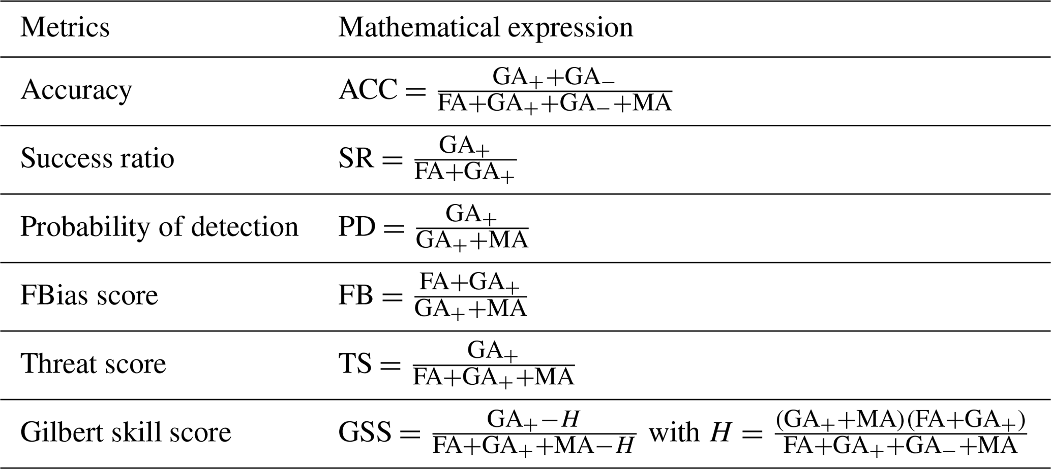
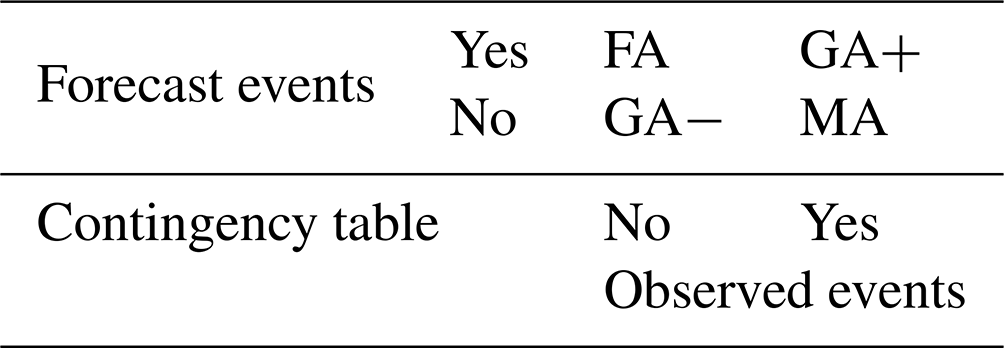
To account for this, the most commonly used threshold indicators (as defined in Table 1) are included in the proposed validation approach, based on the 2×2 contingency table (Table B1, Appendix B) representing the joint distribution of categorical events (below/above the threshold value) predicted by the model and observed by the measurements; i.e. GA+ represents the number of correctly forecasted exceedances, GA− represents the number of correctly forecasted non-exceedances, false alarms (FAs) represent the number of forecasted exceedances that were not observed and missed alarms (MAs) represent the number of observed exceedances that were not forecasted.
All metrics included are listed in Table 1, ranging from 0 to 1, with 1 being the optimal value.
Table 1Categorical metrics included in the validation protocol.
2.3 Assessment of modelling applications' capability to predict air quality indices
One of the main objectives of a forecasting system is to provide citizens with simple information about local air quality and its potential impact on their health, with special regard for sensitive and vulnerable groups (i.e. the very young or old, asthmatics, etc.). Air quality indices (AQIs) are designed to provide information on the potential effects of the different pollutants on people's health by means of a classification of concentration values in terms of qualitative categories.
The AQI outcome is commonly provided by operational forecasting systems; therefore its assessment has been included in the proposed validation approach, by means of a simple multiple threshold assessment, and the number of days predicted by the forecast model in each category is compared with the corresponding number of measured days in more detail.
Of course, the performance assessment depends on the chosen classification table. In the current approach, several AQI tables are available, namely EEA (https://www.eea.europa.eu/themes/air/air-quality-index/index, last access: 20 October 2023), UK Air (https://uk-air.defra.gov.uk/air-pollution/daqi, last access: 20 October 2023; https://uk-air.defra.gov.uk/air-pollution/daqi?view=more-info, last access: 20 October 2023) and the US Environmental Protection Agency (US EPA; https://www.airnow.gov/aqi/aqi-basics/, last access: 20 October 2023; Eder et al., 2010).
The proposed methodology was applied across Europe to evaluate the performances of several forecasting applications. This paper focuses on lessons learnt by the validation of five forecasting applications, based on various methods (in terms of both chemical transport models and statistical approaches) and covering different geographical contexts and spatial scales, from very local to European scales. The key features of the forecast applications are summarized in Table 2. More details are provided for each of them in the following, along with information on the monitoring data used for the validation.
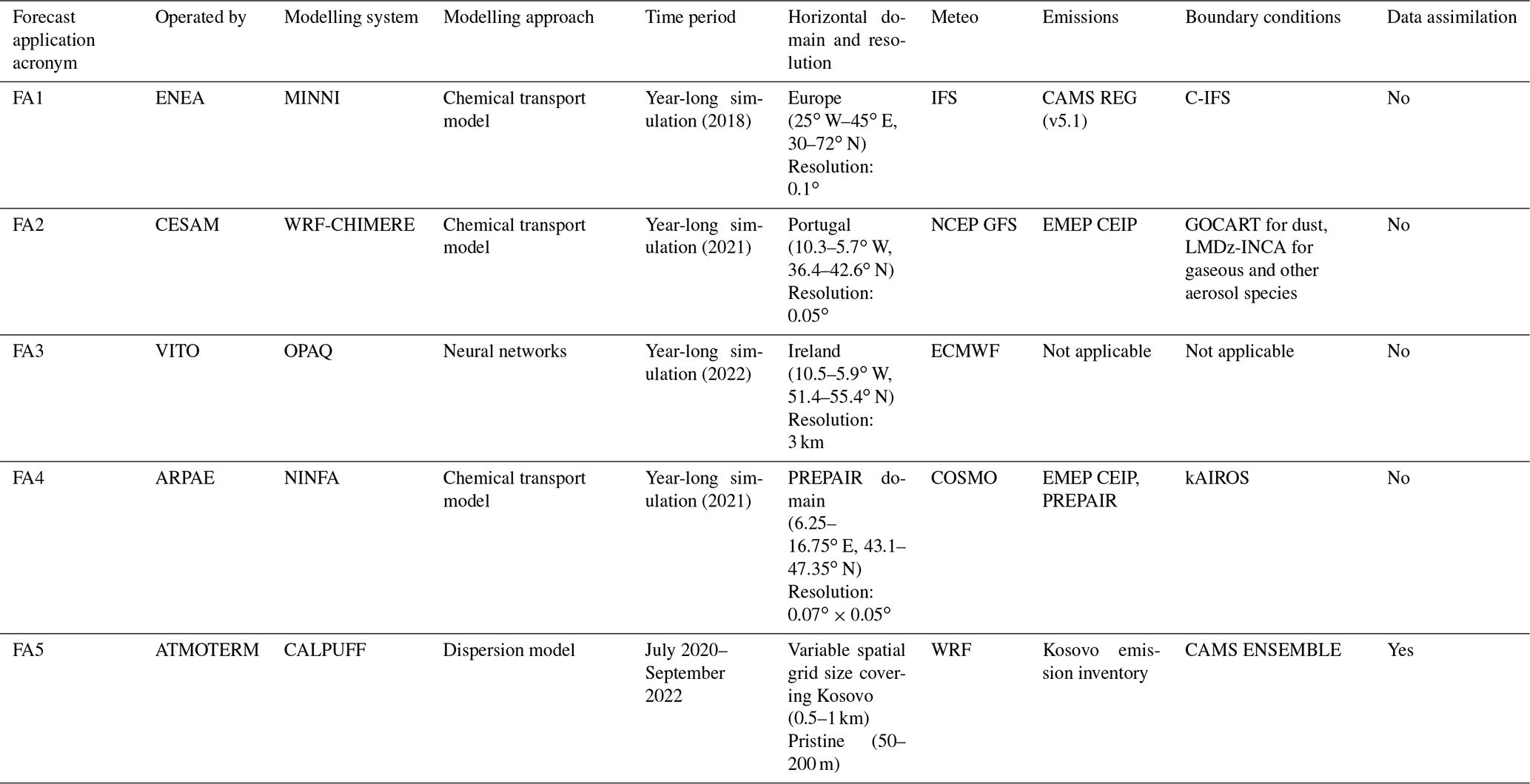
3.1 MINNI simulation over Europe (FA1)
The first forecast application (FA1) was operated by the National Agency for New Technologies, Energy and Sustainable Economic Development (ENEA) applying the MINNI atmospheric modelling system (Mircea et al., 2014; D'Elia et al., 2021) on a European domain at 0.1∘ horizontal spatial resolution. FA1 is a year-long simulation, referring to 2018. MINNI, which has operationally been providing air quality predictions over an Italian domain since 2017 (Adani et al., 2020, 2022), was recently added to the ensemble of the 11 models contributing to the CAMS regional ENSEMBLE production. FA1 was carried out during a preliminary benchmark phase, using CAMS input and setup, but it is not an official CAMS product.
Since no data assimilation was applied within FA1, all available data measured at European background monitoring stations and collected by EEA (E1a at https://discomap.eea.europa.eu/map/fme/AirQualityExport.htm, last access: 20 October 2023) were considered for the validation.
3.2 WRF-CHIMERE simulation over Portugal (FA2)
In Portugal, an air quality modelling system based on the WRF version 3 (Skamarock et al., 2008) and the CHIMERE chemical transport model v2016a1 (Menut et al., 2013; Mailler et al., 2017) has been used for forecasting purposes on a daily basis since 2007 (Monteiro et al., 2005, 2007a, b). The modelling setup comprises three nested domains covering part of northern Africa and Europe, with horizontal resolutions of 125, 25 and 5 km for the innermost domain covering Portugal. At the boundaries of the outermost domain, the outputs from LMDz-INCA (Szopa et al., 2009) are used for all gaseous and aerosol species, and the outputs from the GOCART model are used for dust (Ginoux et al., 2001). The main human activity emissions (traffic, industries and agriculture, among others) are derived based on data from the annual EMEP CEIP emission database (available at https://www.ceip.at/webdab-emission-database/, last access: 20 October 2023), following a procedure of spatial and temporal downscaling. Biogenic emissions are computed online using MEGAN (Guenther et al., 2006), while dust emission fluxes are calculated using the dust production model proposed by Alfaro and Gomes (2001).
Data from the national air quality monitoring network (https://qualar.apambiente.pt, last access: 20 October 2023) are used every year to assess the performance of this forecasting modelling system, usually evaluated on an annual basis. This consists of a group of more than 40 background monitoring stations, classified as urban, suburban and rural, according to the classification settled by European legislation.
3.3 OPAQ simulation over Ireland (FA3)
The OPAQ (Hooyberghs et al., 2005; Agarwal et al., 2020) statistical forecast system has been configured and applied to forecast pollution levels in Ireland by the Irish EPA and VITO. During the configuration stage neural networks are trained at station level with historical observations, ERA5 reanalysis meteorological data and the CAMS air quality forecasts. The forecasts at station level are interpolated to forecast maps for the whole country using the detrended kriging model RIO (Janssen et al., 2008; Rahman et al., 2023), which is part of the OPAQ system.
In this study, we present the historical validation results of a feed-forward neural network model that uses 2 m temperature, vertical and horizontal wind velocity components, CAMS PM10 forecasts, and PM10 observations. More than 2 years of data are used to configure the OPAQ model. Data from October 2019 to June 2022 are used for training. The model is validated on the data for July to December 2022. The testing holdout sample, used to avoid overfitting, covers a time span of 3 months from June to September 2019. The model was optimized using the AdaMax algorithm (Kingma and Ba, 2014) with 4 hidden layers and 200 units per layer; the activation function uses sigmoid functions, while the mean squared error is used as a loss function.
3.4 NINFA simulation over the Po Valley and Slovenia (FA4)
FA4 was operated by the Regional Agency for Prevention, Environment and Energy (ARPAE) applying NINFA, the operational air quality model chain over Po Valley and Slovenia in the framework of the LIFE-IP PREPAIR project (https://www.lifeprepair.eu/, last access: 20 October 2023; Raffaelli et al., 2020). The model suite includes a chemical transport model, a meteorological model and an emissions pre-processing tool. The chemical transport model is CHIMERE, v2017r3. Emission data cover the Po Valley (Marongiu et al., 2022), Slovenia and the other regions/countries present in the model domain (http://www.lifeprepair.eu/wp-content/uploads/2017/06/Emissions-dataset_final-report.pdf, last access: 20 October 2023). The meteorological hourly input is provided by COSMO (http://www.cosmo-model.org, last access: 20 October 2023; Baldauf et al., 2011; Doms and Baldauf, 2018). The boundary conditions are provided by kAIROS (Stortini et al., 2020).
The database of observed data used in this work was built with the support of PREPAIR partners providing revised validated data for 2021.
3.5 CALPUFF simulation over Kosovo (FA5)
FA5 was operated by ATMOTERM between July 2020 and September 2022. Analyses were based on data available from the Kosovo Air Quality Portal hosted by the Hydrometeorological Institute of Kosovo and the Kosovo Open Data Platform (https://airqualitykosova.rks-gov.net/en/, last access: 20 October 2023; https://opendata.rks-gov.net/en/organization/khmi, last access: 20 October 2023). The forecast service used the following modelling tools: the WRF meteorological prognostic model, CAMS ENSEMBLE Eulerian air quality models, and the CALPUFF modelling system with a 1 km receptor grid covering the Kosovo territory and a 0.5 km grid applied in the main cities in Kosovo. In addition a high-resolution receptor network was created for Pristine, with a basic grid step of 50 and 200 m along the roads. The system includes an assimilation module implemented at the post-processing stage using available data from all monitoring stations in Kosovo.
The proposed evaluation methodology for forecasting is in addition to the consolidated FAIRMODE protocol for assessment. The assessment MQO therefore comes first to provide a preliminary evaluation of the five forecasting applications (see Appendix C). This section focuses on the outcomes of applying the additional forecast objectives and criteria and in particular on the lessons learnt by their application in different geographical contexts and on different spatial scales, pointing out the strengths and shortcomings of the approach.
4.1 MQOf skills versus the capability to predict threshold exceedances
Forecast modelling quality objective (MQOf) outcomes are presented here for three forecasting applications, covering different spatial scales, namely FA1 (European scale), FA2 (national scale) and FA4 (regional scale). Along with MQOf outcomes, the skills of the three modelling applications in predicting threshold exceedances are provided as well. We present outcomes for PM10 daily means and O3 daily maximums of 8 h average, since both indicators have a daily limit value set by the current European legislation (European Union, 2008).
Figures 1 and 2, 3 and 4, and 5 and 6 show the outcomes for FA1, FA2 and FA4 applications, respectively. PM10 outcomes are provided in Figs. 1, 3 and 5, while Figs. 2, 4 and 6 present the O3 ones. MQIf values are provided in the forecast target plots (Janssen and Thunis, 2022), at the top of each figure. Within these plots, MQIf is represented by the distance between the origin and a given point (for each monitoring station). Values lower than 1 (i.e. within the green circle) indicate better capabilities than the persistence model (within the measurement uncertainty), whereas values larger than 1 indicate poorer performances. Indeed, the green area identifies the fulfilment of the MQOf at each monitoring station. The MQIf associated with the 90th percentile worst station is reported in the upper-left corner of the plots. This value is used as the main indicator in the proposed benchmarking procedure: its value should be less than or equal to 1 for the fulfilment of the benchmarking requirements. In other words, within the proposed protocol a forecasting application is considered fit for purpose if MQIf is lower than 1 for at least 90 % of the available stations. Note that passing the MQOf test is intended here as a necessary condition for the use of the modelling results, but it must not be understood as a sufficient condition that ensures that model results are of sufficient quality.
The outcomes of all categorical metrics included in the validation protocol are provided at the bottom of each figure, by means of the forecast summary p-normalized reports. Within these plots, the statistical distributions (5th, 25th, 50th, 75th, 95th percentiles) of the outcomes of all the indicators defined in Sect. 2.2 are summarized and compared with the corresponding outcomes of the persistence model (i.e. the ratios of the skills are considered). The green area indicates that the model performs better than the persistence model for that particular indicator.
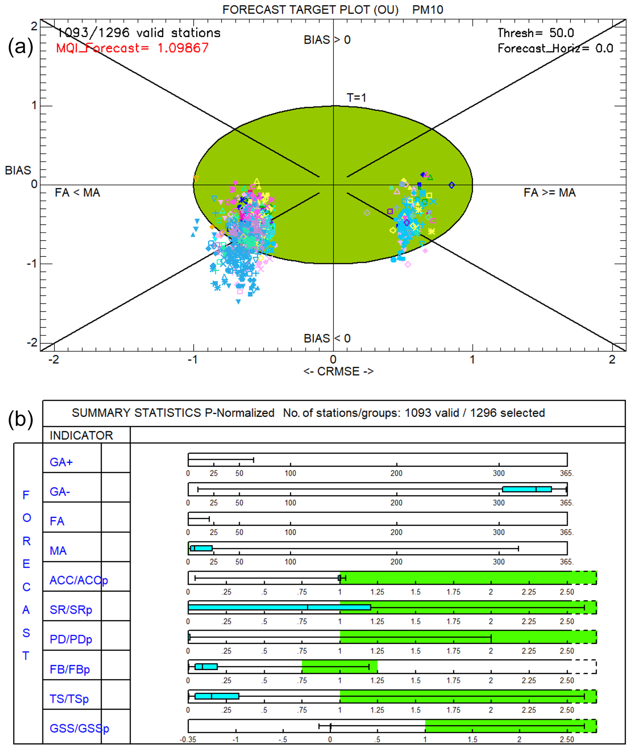
Figure 1FA1 validation outcomes for PM10. The forecast target plots (a) provide the MQIf values for each monitoring station, as the distance between the origin and a given point. The boxplots in the forecast summary p-normalized reports (b) provide the statistical distribution (5th, 25th, 50th, 75th, 95th percentiles) of the categorical metrics.
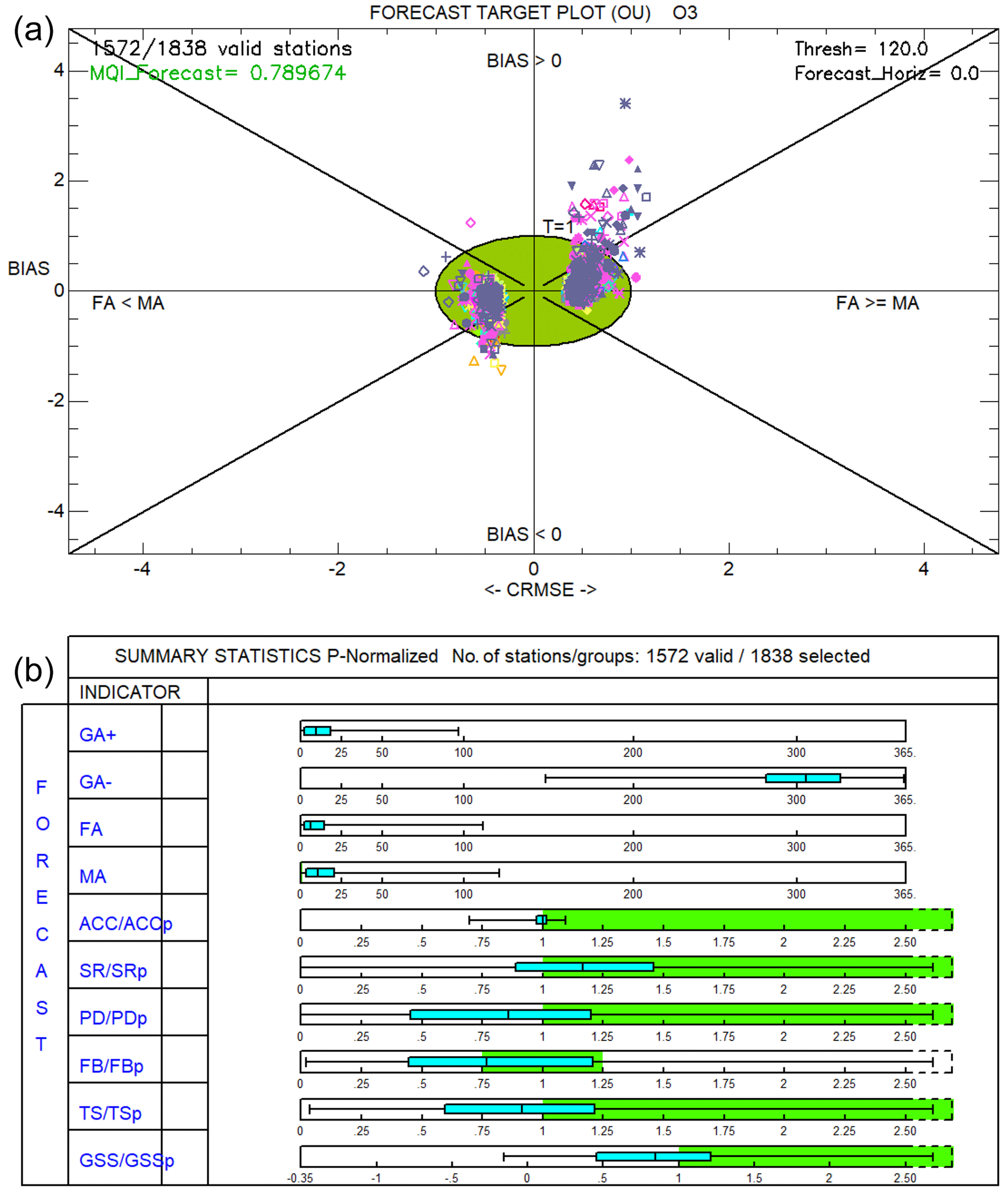
Figure 2FA1 validation outcomes for O3. The forecast target plots (a) provide the MQIf values for each monitoring station, as the distance between the origin and a given point. The boxplots in the forecast summary p-normalized reports (b) provide the statistical distribution (5th, 25th, 50th, 75th, 95th percentiles) of the categorical metrics.
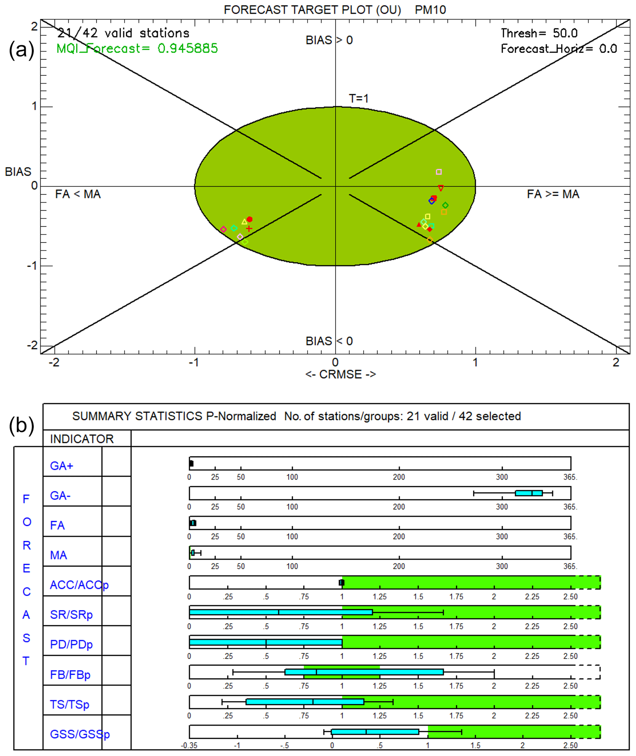
Figure 3FA2 validation outcomes for PM10. The forecast target plots (a) provide the MQIf values for each monitoring station, as the distance between the origin and a given point. The boxplots in the forecast summary p-normalized reports (b) provide the statistical distribution (5th, 25th, 50th, 75th, 95th percentiles) of the categorical metrics.
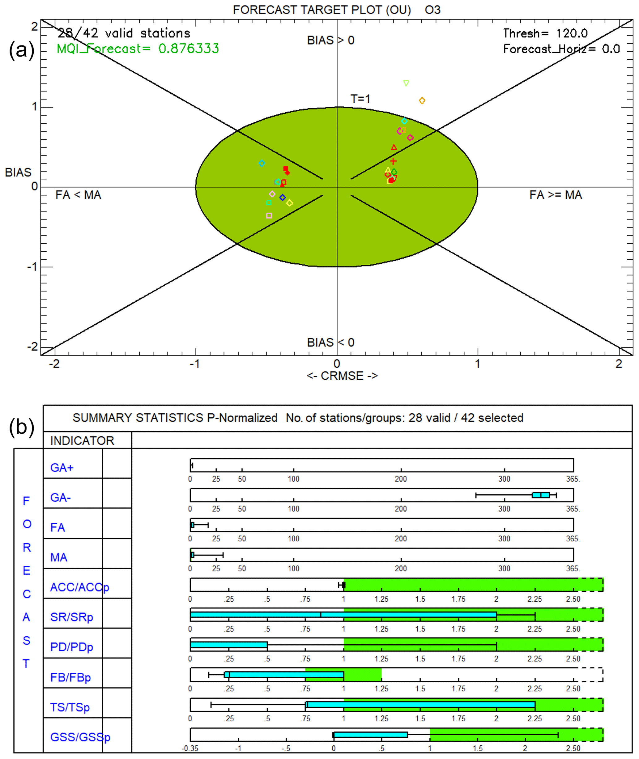
Figure 4FA2 validation outcomes for O3. The forecast target plots (a) provide the MQIf values for each monitoring station, as the distance between the origin and a given point. The boxplots in the forecast summary p-normalized reports (b) provide the statistical distribution (5th, 25th, 50th, 75th, 95th percentiles) of the categorical metrics.
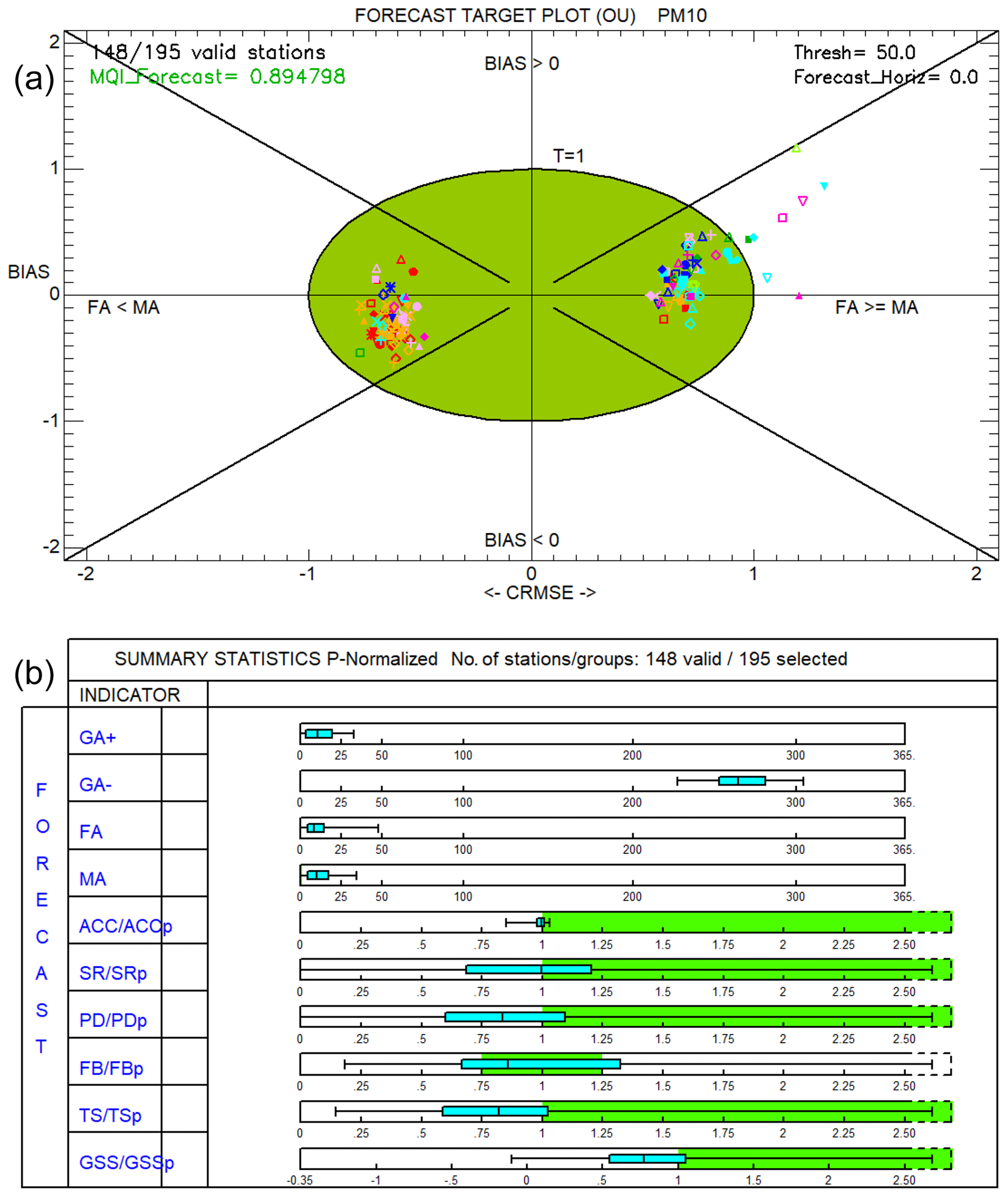
Figure 5FA4 validation outcomes for PM10. The forecast target plots (a) provide the MQIf values for each monitoring station, as the distance between the origin and a given point. The boxplots in the forecast summary p-normalized reports (b) provide the statistical distribution (5th, 25th, 50th, 75th, 95th percentiles) of the categorical metrics.
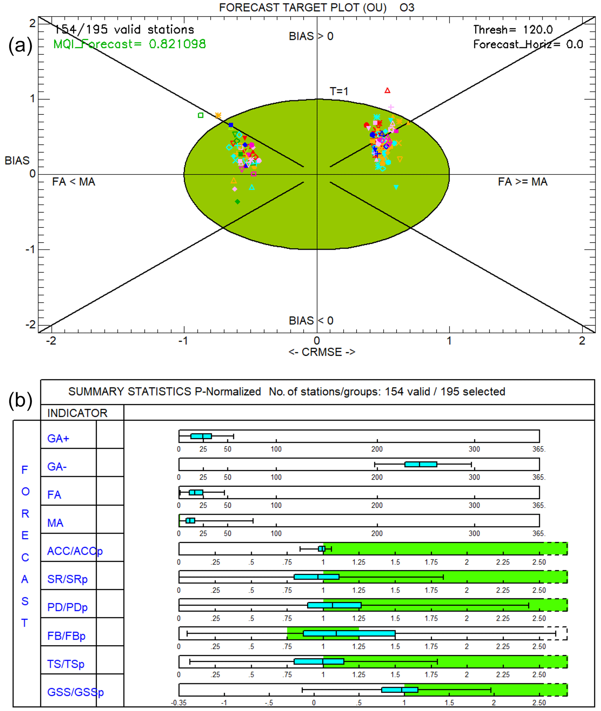
Figure 6FA4 validation outcomes for O3. The forecast target plots (a) provide the MQIf values for each monitoring station, as the distance between the origin and a given point. The boxplots in the forecast summary p-normalized reports (b) provide the statistical distribution (5th, 25th, 50th, 75th, 95th percentiles) of the categorical metrics.
Forecast target plot outcomes indicate a very good level of quality of all forecast applications in simulating O3. The 90th percentile of the MQIf values is lower than 1 for all three forecast applications, indicating that the model performs better than the persistence model in simulating O3 at more than 90 % of the available stations. FA2 and FA4 also fulfil the MQIf requirements in simulating PM10, but there is room for improvement for the European-scale simulation FA1 (the 90th percentile of the MQIf values is slightly higher than 1). Further investigations show that most of the issues emerge in a limited part of the modelling domain (Turkey), where very high, and sometimes unlikely, PM10 values are measured at several monitoring sites for most of the year. By removing Turkish monitoring stations from the validation data set, MQOf turns out to be fulfilled (Fig. D1, Appendix D). It is worth noting that the MQOf outcomes are consistent with the standard assessment evaluation (Appendix C). Table C1 shows that the standard MQO is fulfilled for all O3 forecast applications. For PM10, the MQI is higher than 1 but only for the FA1 simulation.
Concerning the capability to predict exceedances, model performances improve moving from FA1 to FA4 applications (i.e. as spatial resolution increases), and skills are generally better at simulating O3 than PM10. Concerning the comparison of the performances according to the different metrics, all forecast applications turn out to be better at avoiding false alarms than at reproducing all of them, since success ratio (SR) scores are generally better than probability of detection (PD) ones, especially for PM10.
In general, even if forecast applications are generally better than the persistence model according to the main outcome MQOf (top plots of Figs. 1–6), it becomes harder for them to beat the persistence model at predicting exceedances (bottom plots of Figs. 1–6). Apart from a few cases (namely the regional FA4 application), the median values of the statistical distribution of the outcomes are not in the green area, indicating that the model performs worse than the persistence model at more than 50 % of the available stations.
4.2 MPI plot supporting the interpretation of MQOf outcomes
When evaluating a forecasting application, it is important to assess the evolution of skill metrics with the forecast horizon. Indeed, a good forecasting application should not incur a substantial degradation of its performances along with forecast time.
FA3, carried out over Ireland by means of the OPAQ statistical system, was evaluated for each of the forecasted days, which included the current day (day0), tomorrow (day1) and the day after tomorrow (day2).
In the following it is reported how performances in simulating PM10 vary along with the forecast days. Outcomes for day0 and day2 are shown in more detail in Figs. 7 and 8, respectively. On the top of each figure, the forecast target plots (described in the previous section) are reported. On the bottom, the forecast MPI plots are added, describing the fulfilment of both criteria defined in Sect. 2.1 (i.e. MPI less than or equal to 1). Indeed, here the forecast performances (MFEf) are compared with the persistence model performances (MFEp) along the y axis (MPI1) and with the mean fractional uncertainty (MFU) along the x axis (MPI2). The green area identifies the area of fulfilment of both proposed criteria. The orange areas indicate where only one of them is fulfilled.
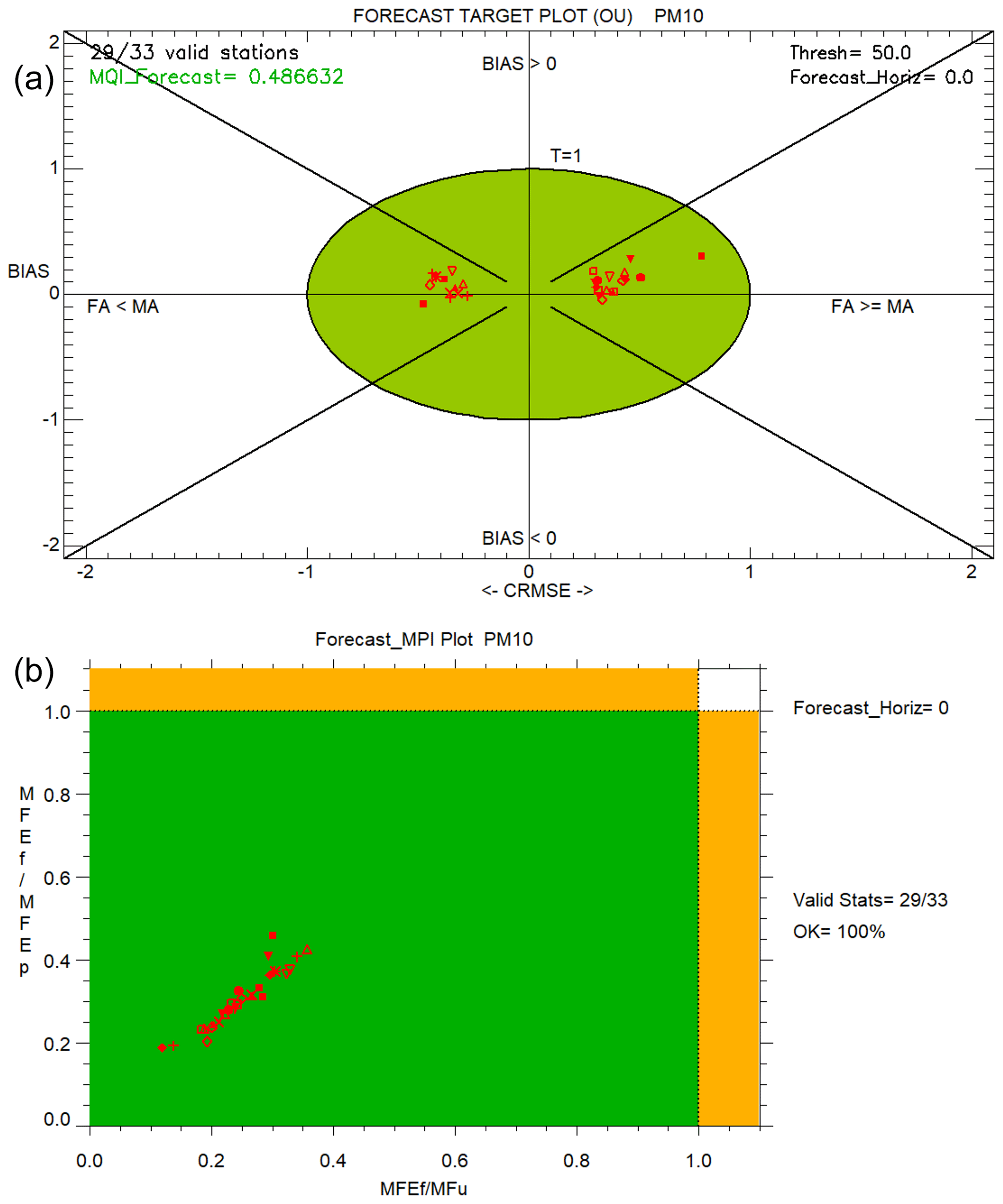
Figure 7FA3 validation outcomes for day0. The forecast target plots (a) provide the MQIf values for each monitoring station, as the distance between the origin and a given point. The forecast MPI plots (b) provide MPI1 and MPI2 values for each monitoring station along the y and x axes, respectively.
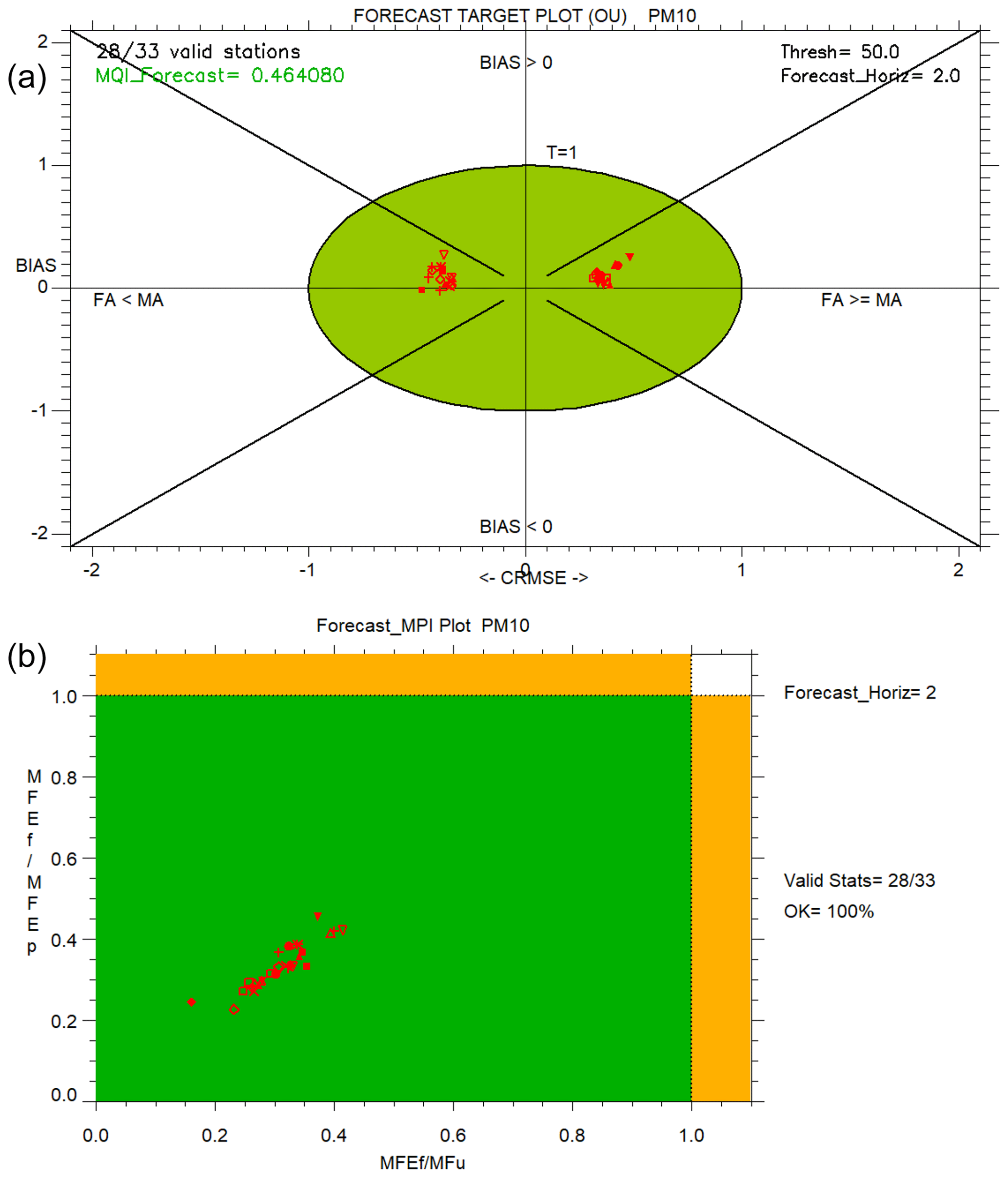
Figure 8FA3 validation outcomes for day2. The forecast target plots (a) provide the MQIf values for each monitoring station, as the distance between the origin and a given point. The forecast MPI plots (b) provide MPI1 and MPI2 values for each monitoring station along the y and x axes, respectively.
The outcomes in Figs. 7–8 indicate a very good level of quality of the forecast application, since the modelling quality objective is fulfilled (top), together with the two additional performance criteria (bottom). These outcomes are consistent with the standard MQO skills provided in Table C1 of Appendix C, which points out very good performances of FA3 for PM10, namely the best performances among all forecast applications.
Concerning the evolution of skill metrics with the forecast horizon, according to the forecast target plot outcomes (top), modelling performances unexpectedly get better from day0 to day2, since the MQIf value associated with the 90th percentile worst station (reported in the upper-left corner of the plots) becomes lower. According to the forecast MPI plots (bottom), performances remain almost constant with the forecast horizon, indicative of a good behaviour of the modelling application. Moreover, forecast MPI plots help to clarify that the unrealistic improvement in model performances from day0 to day2, pointed out by the forecast target plots, is due to the persistence model performance degradation. Indeed, moving from day0 to day2, the forecast model performances get slightly better along the y axis, where they are normalized to the persistence model's skills, but they deteriorate slightly along the x axis, where they are considered regardless of persistence aspects. In other words, model performances deteriorate slightly along with the forecast days, but the persistence model deteriorates more so that performance ratios (i.e. both MQIf and MPI1 values) become lower.
4.3 Assessment of modelling applications' capability to predict air quality indices
The current approach for assessing modelling applications' capability to predict air quality indices is based on a cumulative analysis for answering the following questions: are citizens correctly warned against high-pollution episodes? Or, in another words, does the model properly forecast AQI levels?
Air quality indices are designed to provide information on local air quality. Moreover, within the proposed validation protocol, the capability to correctly predict AQIs is assessed at single monitoring stations. For these reasons, FA5 at the local scale is the most suitable for testing the proposed approach. Indeed, it was carried out at high spatial resolution and focused on only two monitoring sites, located in two cities in Kosovo: Pristine (the capital) and Drenas.
Before analysing the AQI results for PM2.5, it has to be mentioned that the FA5 standard MQO is fulfilled for all available pollutants (Table C1, Appendix C). Concerning additional features of the forecasting validation protocol, both the forecast target plot and the forecast MPI plot show very good performances for both locations. The forecast summary p-normalized report indicates good model performance in Drenas and some room for improvement in Pristine due to underestimation of PM2.5 episodes.
Figure 9 provides the AQI diagram, based on EEA classification, for PM2.5 and the day0 forecast. For each station, the bar plot shows two paired bars: the number of predicted (left bar) and measured (right bar) concentration values that fall within a given air quality category. In Drenas, forecast values populate categories 2 (“good”), 3 (“medium”) and 4 (“poor”) to a greater extent than the measurements. On the contrary, in Pristine forecast values are more frequent than the measurements at the lowest AQI (“very good”).
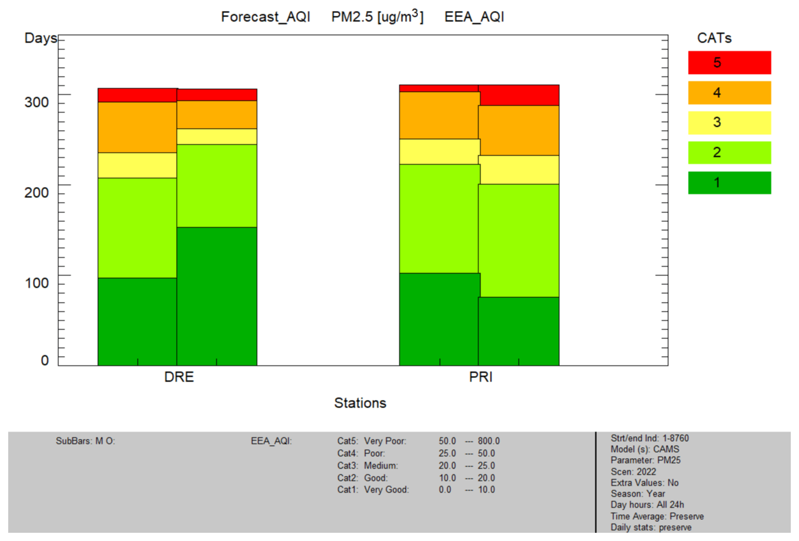
Figure 9FA5 validation outcomes for PM2.5 at Drenas and Pristina. The AQI diagram provides for each monitoring station the number of predicted (left bar) and measured (right bar) concentration values that fall within each air quality category. The last two EEA AQI classes (very poor and extremely poor) are merged into one.
Overall, Fig. 9 points out that FA5 generally overestimates PM2.5 concentration levels in Drenas and underestimates them in Pristine. The AQI forecast bar plots provide information about the total number of occurrences in each AQI class, but there is no information about the correct timing of the forecasted AQI level.
So, there is room for future improvement, and other additional outputs could be included within the protocol. In particular, multi-category contingency tables can be created for each station, and multi-categorical skill scores can be computed, according to the literature (e.g. EPA, 2003). Outcomes can be plotted for single stations or skill score statistical distributions among the stations can be described for each AQI class.
For example, in Fig. 10 an in-depth insight into AQI assessment is proposed for Drenas (top) and Pristina (bottom). Two additional multi-categorical metrics are proposed. Both of them are computed for each AQI level and are based on the comparison between forecast and measurement values also considering the correct timing of the predicted AQI level. AQI comparability (left plots in Fig. 10) represents, for each of the five AQI classes, the percentage of the correct forecast events in this class with respect to the total events based on measurements. Since AQI comparability values are percentages, they range from 0 to 100, with 100 being the optimal value. TS_AQI (right plots in Fig. 10) is computed according to the same definition of TS in Table 1. Indeed, here multiple thresholds (i.e. class limits) are taken into account, and so multiple outcomes, one for each AQI class, are provided. TS_AQI values range from 0 to 1, with 1 being the optimal value.
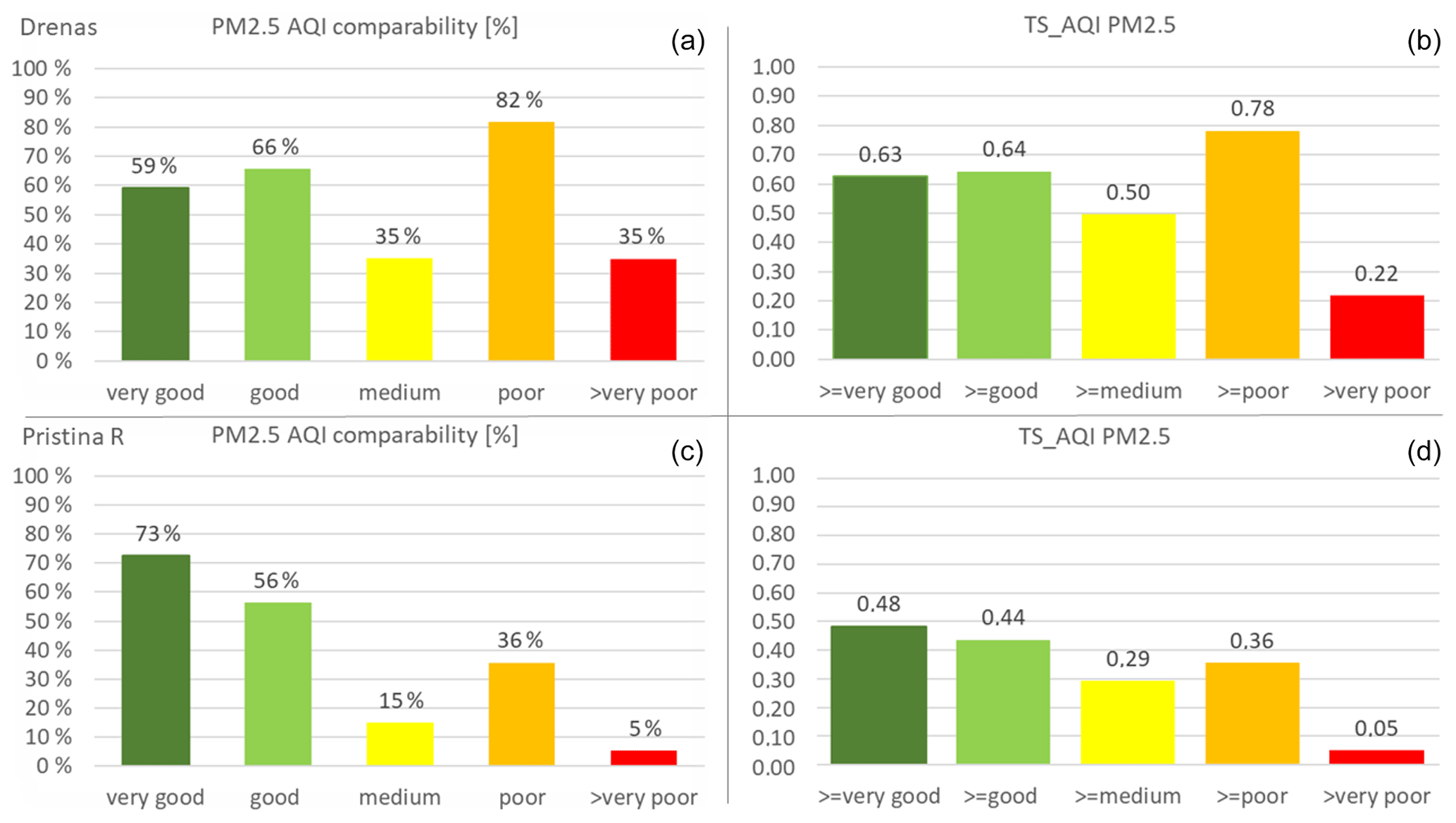
Figure 10Multi-categorical metric outcomes for Drenas (a, b) and Pristina (c, d). The AQI comparability plots (a, c) provide for each AQI class the percentage of the correct forecast events with respect to the total events based on measurements. TS_AQI plots (b, d) provide TS_AQI values for each AQI class.
AQI comparability and TS_AQI in Fig. 10 provide additional information with respect to the AQI diagram. For example, in the case of Drenas, it is shown that, according to both metrics, the best agreement between forecast and measurements in predicting the correct timing of the occurrences is found for the poor AQI class. It is also worth noting that, even if according to cumulative analysis (Fig. 9) forecast and measurements present a similar number of occurrences in both the medium and the very poor classes, according to AQI comparability, these classes are characterized by the worst performances. TS_AQI gives additional information about the model performances, which is especially noticeable for the medium and very poor classes, as it defines levels differently (the medium class includes medium and all higher classes, i.e. poor and very poor). In this case the medium class is characterized by better performances than the very poor class. In the case of Pristine, the best performances, according to both metrics, are achieved for low concentrations (very good and good classes) and the worst ones for very poor and medium AQI levels. It is also worth noting that the best agreement is found for the good class, according to the cumulative comparison (Fig. 9), but it is better for the very good class if the timing of the occurrences is taken into account (Fig. 10).
4.4 Discussion
Several lessons were learnt from the results presented here. The main proposed criterion (MQOf) turned out to be useful for evaluating the strengths and shortcomings of a forecasting application, focusing on features which could not be addressed with the assessment evaluation approach.
Side outcomes, included within the protocol, can help to deepen the analysis. For example, MPI analysis based on MFE helps to interpret the outcomes, since MPI2 is formulated regardless of persistence aspects, providing details on the model performances.
Consistently with the FAIRMODE approach, the measurement uncertainty is considered within the MQOf formulation. While values are currently based on maximum uncertainties (95th percentile), these could be modified in the future to obtain a consensus level of stringency for the MQOf, i.e. a level reachable for the best applications while stringent enough to preserve sufficient quality. In Appendix E the outcomes of a sensitivity analysis are provided, in which we investigate the impact of the value chosen as representative for measurement uncertainty.
Concerning the capability to predict the exceedances, it turned out that, regardless of the spatial scale and pollutants, even if a forecast application is better than the persistence model according to the general evaluation criterion (MQOf), it can be worse at correctly providing categorical answers. Indeed, the difficulty in beating the persistence model skills is not infrequent in weather forecasting applications (Mittermaier, 2008). Moreover, it is worth noting that, differently from MQOf analysis, the evaluation of the model's capability to predict the exceedances, being based on the definition of fixed thresholds, does not take the measurement uncertainty into account. For these reasons, a fitness for purpose criterion concerning exceedance metrics (e.g. which percentiles of a categorical indicator should be in the green area in order to define its skill as “good enough”? And following this, how many indicators should be good enough in order to define the forecast application as fit for purpose?) is not definitively set within the proposed protocol. Indeed, more discussions based on further tests on forecasting applications are needed.
The greatest room for improvement concerns the evaluation of the capability of the forecasting application to predict AQI levels. The current approach is based on a cumulative analysis, and no information is provided about the correct timing of the forecasted AQI levels. To account for this, some preliminary tests were carried out based on two additional multi-categorical metrics, which sound interesting with respect to complementing the current approach. The main weakness of the proposed approach is the large number of different values to be provided, thus making this type of outcome usable only for single monitoring stations. Moreover, the question of which level of performances in AQI predicting is good enough is currently an open issue, and benchmarking of several forecasting applications is needed to establish some quality criteria.
A standardized validation protocol for air quality forecast applications was proposed, following FAIRMODE community discussions on how to address specific issues typical of forecasting applications.
The proposal of a common benchmarking framework for model developers and users supporting policymaking under the European Ambient Air Quality Directives is a major achievement.
The proposed validation protocol enables an objective assessment of the fitness for purpose of a forecasting application, since it relies on the usage of a reference forecast as a benchmark (i.e. the persistence model), includes the measurement uncertainty and bases the evaluation on the fulfilment of specific performance criteria defining an acceptable quality level of the given model application. On top of a pass–fail test to ensure fitness for purpose (intended as a necessary but not sufficient condition), a series of indicators is proposed to further analyse the strengths and weaknesses of the forecast application.
Moreover, relying on a common standardized validation protocol, the comparison of performances of different forecast applications, within a common benchmarking framework, is made available.
The application of the methodology to validate several forecasting simulations across Europe, using different modelling systems and covering various geographical contexts and spatial scales, suggested some general considerations about its usefulness.
The main fitness for purpose criterion, describing the global performances of the model application with respect to persistence skills, proves to be useful for a comprehensive evaluation of the strengths and shortcomings of a forecasting application. Generally, the forecast modelling quality objective turns out to be achievable for most of the examined validation exercises. When the criterion was not addressed, side analyses and outcomes, included within the protocol, helped to deepen the analysis and to identify the most critical issues of the forecasting application.
On the other hand, it turned out that, regardless of the spatial scale and the pollutants, it can be hard for a forecast application to beat the persistence model skills at correctly providing categorical answers, namely on exceedances of concentration thresholds. Therefore, further tests and analyses are needed in order to provide some criteria for defining the fitness for purpose of a forecasting application in predicting exceedances.
The last model capability assessed within the proposed validation protocol concerns the correct prediction of air quality indices, designed to provide citizens with effective and simple information about air quality and its impact on their health. The current approach is based on a cumulative analysis of relative distributions of observed and forecasted AQIs. As no information is provided about the correct timing of the forecasted AQI levels, further developments are foreseen based on multi-category contingency tables and multi-categorical skill scores.
Discussion on the proposed approach will continue within the FAIRMODE community, and upgrades and improvements of the current validation protocol will be fostered by its usage. In particular, it will be of interest to collect feedback from in-depth diagnostic analyses focusing on the validation of specific forecast applications, using both the proposed criteria and the threshold-based categorical metrics to gain further insights. From its preliminary applications across Europe, the methodology has turned out to be sufficiently robust for testing and application, especially with respect to targeting air quality forecasting services supporting policymaking in European member states.
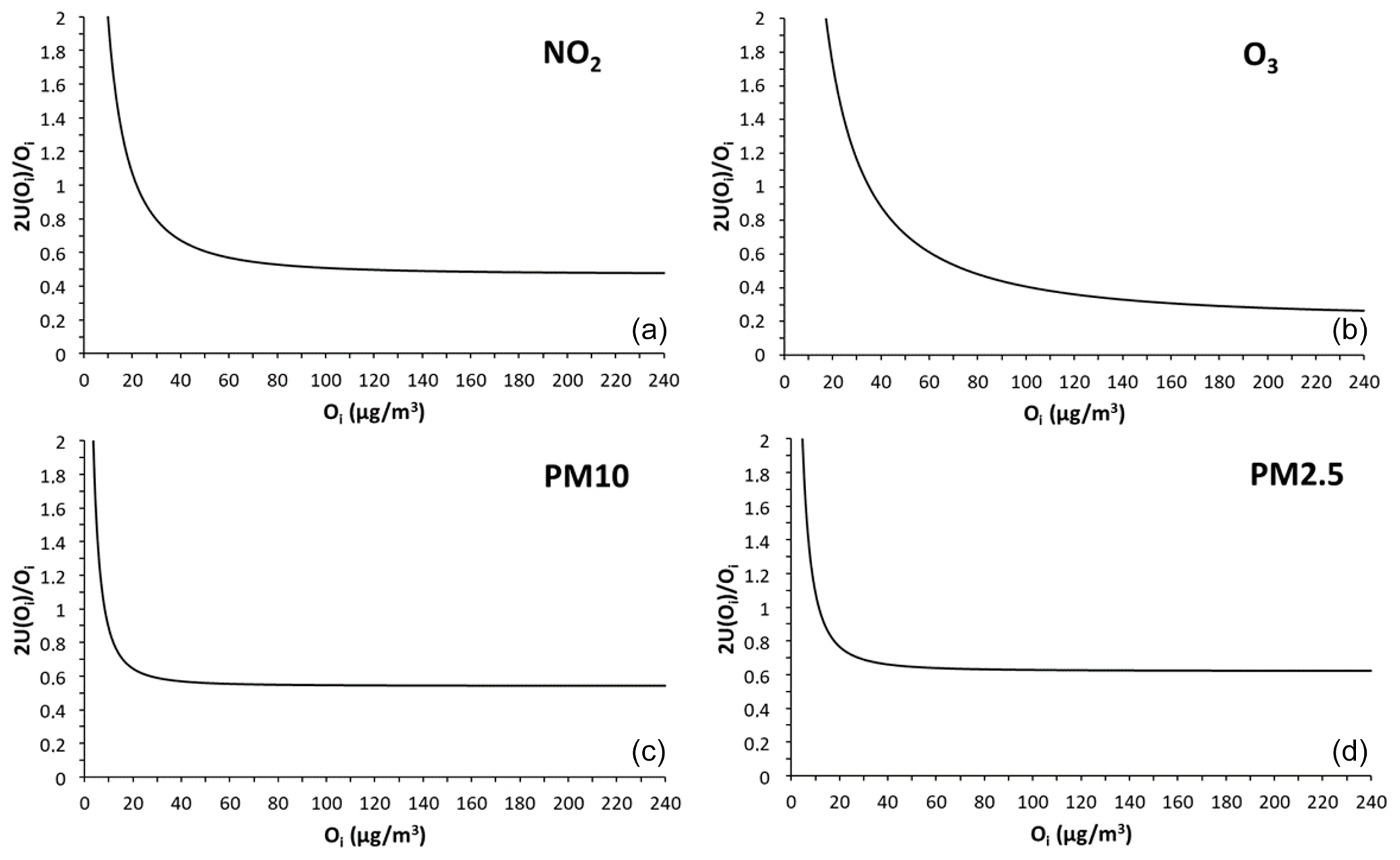
Figure A1Double relative measurement uncertainties as a function of concentration values for NO2 (a), O3 (b), PM10 (c) and PM2.5 (d).
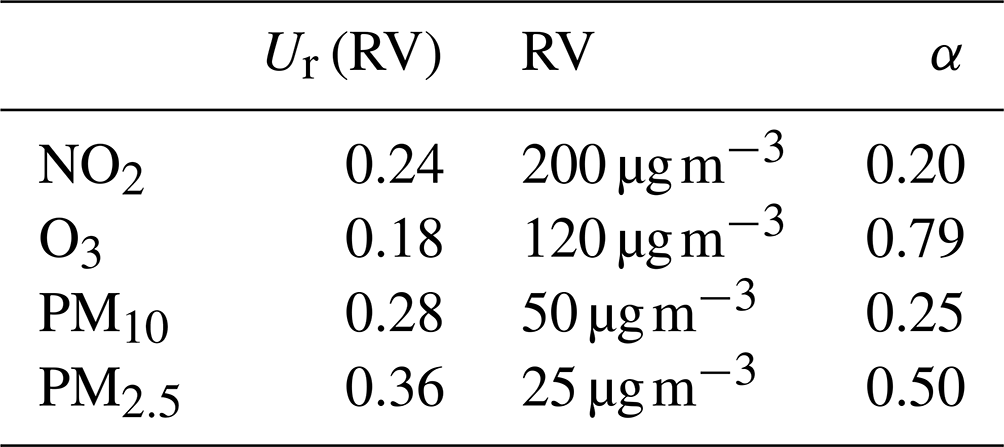
Table A1Parameters for the calculation of measurement uncertainty.
Measurement uncertainty U(Oi) as a function of the concentration values Oi can be expressed as follows:
An in-depth description of the rationale and formulation of the measurement uncertainty estimation is provided in Thunis et al. (2013) for O3 and in Pernigotti et al. (2013) for PM and NO2. The formulation of the measurement uncertainty as a function of the measured concentration is based on two coefficients: Ur(RV), i.e. the relative uncertainty around a reference value RV, and α, i.e. the fraction of uncertainty not proportional to the concentration value. It is important to note that we use as representative for the measurement uncertainty the 95th percentile highest value among all uncertainty values. For PM10 and PM2.5 the results of the JRC instrument inter-comparison (Pernigotti et al., 2013) have been used, whereas a set of EU AirBase stations available for a series of meteorological years has been used for NO2, and analytical relationships have been used for O3. These 95th percentile uncertainties only include the instrumental error. Ur(RV), RV and α for U(Oi) calculation of NO2, O3 and PM are provided in Table A1.
The standard modelling quality objective (MQO), valid for assessment, is defined by the comparison of model–observation differences (namely the root mean square error, RMSE) with a quantity proportional to the measurement uncertainty.
β is set to 2, thus allowing the deviation between modelled and observed concentrations to be twice the measurement uncertainty. The measurement uncertainty U(Oi) as a function of the concentration values Oi is defined in Appendix A.
MQO is fulfilled when MQI is less than or equal to 1.
Standard assessment MQO outcomes (i.e. MQI value associated with the 90th percentile worst station) for all available pollutants are summarized in Table C1 for all forecast applications.
Table C1Standard assessment MQI values (associated with the 90th percentile worst station) for all forecast applications.
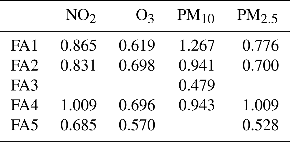
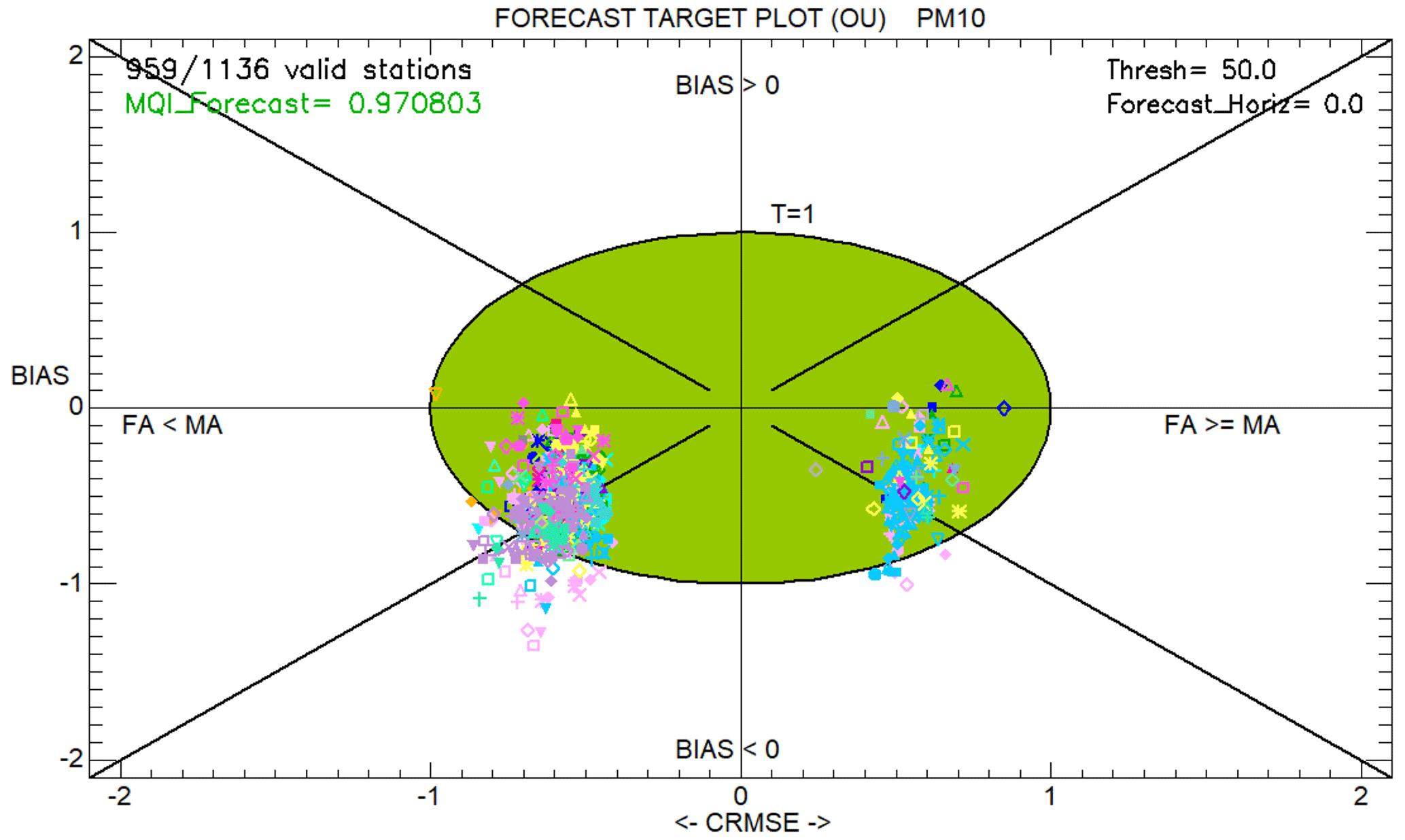
Figure D1FA1 forecast target plot for PM10, removing Turkish monitoring stations from the validation data set.
The effect on MQIf outcomes of lowering measurement uncertainty estimates is investigated here. The values of Ur(RV) parameters in Table A1 (i.e. the estimates of the relative uncertainty around the reference value, defining the asymptotic behaviour of the functions of Fig. A1) were reduced by 25 % and 50 % for all the pollutants, and the MQIf were recalculated for the different forecast applications. Figure E1 shows the results for all available data: FA1, FA2 and FA4 outcomes for the current forecast day (all pollutants available) and FA3 outcomes along a 3 d forecast horizon (only PM10 available). Different colours refer to results based on different Ur(RV) values: 1 Ur(RV) indicates the original values in Table A1; 0.75 Ur(RV) and 0.50 Ur(RV) refer to 25 % and 50 % reductions, respectively. Indeed, the 50 % reduction decreases the Ur(RV) values to 0.12 (NO2), 0.09 (O3), 0.14 (PM10) and 0.18 (PM2.5), i.e. well below the data quality objective values set by the current European legislation (European Union, 2008), namely 15 % for NO2 and O3 and 25 % for particulate matter.
The results of the sensitivity analysis are provided by means of violin plots (Hintze and Nelson, 1998), showing the distributions of the MQIf values computed for each monitoring station. In other words, each violin refers to all the data provided within the corresponding forecast target plot, giving in a single plot an overall view of all the outcomes available. Three lines were added to the display of each violin, indicating the 10th, 50th and 90th percentiles of the distributions.
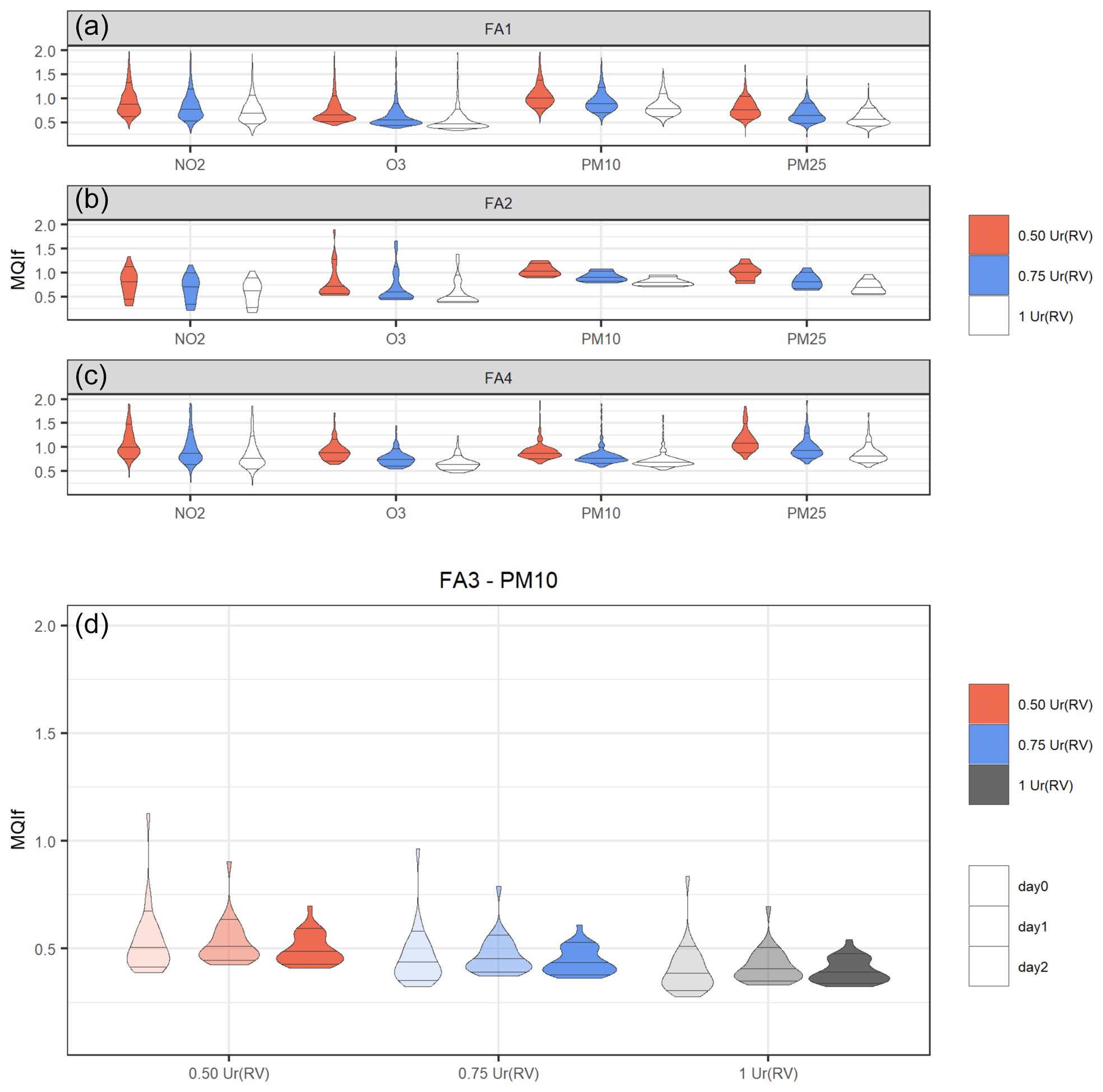
Figure E1The effect of lowering Ur(RV) on the distribution of MQIf values. (a–c) FA1, FA2 and FA4 outcomes for the current forecast day (all the pollutants available). (d) FA3 outcomes along a 3 d forecast horizon (only PM10 available).
The results show that both MQIf values and the shape of their distribution depend on both the forecast application and the pollutant. Within this context, changing Ur(RV) values induces a very slight effect on the shape of the MQIf value distribution, apart from the case of PM2.5 for FA2, where a small amount of data are available (11 monitoring stations). On the contrary, as expected, changing Ur(RV) values result in variations in MQIf values, which increase as Ur(RV) decreases, to a different extent depending on the forecast application and the pollutant. Generally, variations tend to be lower if data availability is higher. Concerning the main MQOf criterion fulfilment (i.e. the 90th percentile of the MQIf values is lower than 1), being based on a categorical answer (yes/no), it changes or not mainly depending on the performances of the reference analysis (1 Ur(RV)). The same answer is maintained both in the case of very good performances (MQIf 90th percentile value largely lower than 1) and in the case of the criterion not being fulfilled even in the reference analysis (MQIf 90th percentile value already higher than 1). If the MQIf 90th percentile value is lower but quite close to 1, the MQOf criterion fulfilment is of course more sensitive to measurement uncertainty estimates. Indeed, this is expected, and it is a typical shortcoming of the usage of criteria based on categorical answers.
The DELTA Tool software and all data sets generated and analysed during the current study are available on Zenodo at https://doi.org/10.5281/zenodo.7949868 (Thunis and Vitali, 2023).
KC, PD, SJ, AM, AP, PT and LV contributed to the study conception and design. PT conceived part of the methodology, and KC developed the software. Material preparation, data collection and analysis were performed by MA, RA, AB, AD'A, CG, GG, AM, TP, MS, LV and SV. The first draft of the manuscript was written by AM, AP and LV, and all authors commented on previous versions of the manuscript. All authors read and approved the final paper.
The contact author has declared that none of the authors has any competing interests.
Publisher's note: Copernicus Publications remains neutral with regard to jurisdictional claims made in the text, published maps, institutional affiliations, or any other geographical representation in this paper. While Copernicus Publications makes every effort to include appropriate place names, the final responsibility lies with the authors.
The analysis for the Irish air quality forecasts has been supported by the LIFE Emerald project Emissions Modelling and Forecasting of Air in Ireland. VITO thanks the Irish EPA for sharing all observation data and for continuous valuable feedback on the model developments.
The NINFA simulation over the Po Valley and Slovenia was developed under the project LIFE-IP PREPAIR (Po Regions Engaged to Policies of AIR), which was co-funded by the European Union LIFE programme in 2016, under grant number LIFE15 IPE/IT/000013. Acknowledgements are given to all the beneficiaries of the LIFE-IP PREPAIR project: the Emilia-Romagna (project coordinator), Veneto, Lombardy, Piedmont, and Friuli Venezia Giulia regions; the Autonomous Province of Trento; the Regional Agency for Prevention, Environment and Energy Emilia-Romagna; the Regional Agency for Environmental Prevention and Protection of Veneto; the Regional Agency for the Protection of the Environment of Piedmont; the Regional Agency for Environmental Protection of Lombardy; the Environmental Protection Agency of Valle d'Aosta; the Environmental Protection Agency of Friuli Venezia Giulia; the Slovenian Environment Agency; the municipality of Bologna; the municipality of Milan; the city of Turin; ART-ER; and the Lombardy Foundation for the Environment.
The forecasts for Kosovo were developed under the Supply of Project Management, Air Quality Information Management, Behaviour Change and Communication Services project managed by the Millennium Foundation Kosovo (MFK), funded by the Millennium Challenge Corporation (MCC). Acknowledgements are given to all the beneficiaries and participants of the project for Kosovo, including the Millennium Foundation Kosovo, the Hydrometeorological Institute of Kosovo and the National Institute of Public Health of Kosovo.
This research has been supported by the European Union (grant nos. LIFE19 GIE/IE/001101 and LIFE15 IPE/IT/000013). FCT/MCTES supported the contract granted to Carla Gama (2021.00732.CEECIND) and the CESAM Associated Laboratory (UIDB/50017/2020 and UIDP/50017/2020).
This paper was edited by Jason Williams and reviewed by three anonymous referees.
Adani, M., Piersanti, A., Ciancarella, L., D'Isidoro, M., Villani, M. G., and Vitali, L.: Preliminary Tests on the Sensitivity of the FORAIR_IT Air Quality Forecasting System to Different Meteorological Drivers, Atmosphere, 11, 574, https://doi.org/10.3390/atmos11060574, 2020.
Adani, M., D'Isidoro, M., Mircea, M., Guarnieri, G., Vitali, L., D'Elia, I., Ciancarella, L., Gualtieri, M., Briganti, G., Cappelletti, A., Piersanti, A., Stracquadanio, M., Righini, G., Russo, F., Cremona, G., Villani, M. G., and Zanini, G.: Evaluation of air quality forecasting system FORAIR-IT over Europe and Italy at high resolution for year 2017, Atmos. Pollut. Res., 13, 101456, https://doi.org/10.1016/j.apr.2022.101456, 2022.
Agarwal, S., Sharma, S., R., S., Rahman, M. H., Vranckx, S., Maiheu, B., Blyth, L., Janssen, S., Gargava, P., Shukla, V. K., and Batra, S.: Air quality forecasting using artificial neural networks with real time dynamic error correction in highly polluted regions, Sci. Total Environ., 735, 139454, https://doi.org/10.1016/j.scitotenv.2020.139454, 2020.
Alfaro, S. C. and Gomes, L.: Modeling mineral aerosol production by wind erosion: Emission intensities and aerosol size distributions in source areas, J. Geophys. Res.-Atmos., 106, 18075–18084, https://doi.org/10.1029/2000JD900339, 2001.
Bai, L., Wang, J., Ma, X., and Lu, H.: Air Pollution Forecasts: An Overview, Int. J. Environ. Res. Publ. He., 15, 780, https://doi.org/10.3390/ijerph15040780, 2018.
Baklanov, A. and Zhang, Y.: Advances in air quality modeling and forecasting, Glob. Transit., 2, 261–270, https://doi.org/10.1016/j.glt.2020.11.001, 2020.
Baklanov, A., Schlünzen, K., Suppan, P., Baldasano, J., Brunner, D., Aksoyoglu, S., Carmichael, G., Douros, J., Flemming, J., Forkel, R., Galmarini, S., Gauss, M., Grell, G., Hirtl, M., Joffre, S., Jorba, O., Kaas, E., Kaasik, M., Kallos, G., Kong, X., Korsholm, U., Kurganskiy, A., Kushta, J., Lohmann, U., Mahura, A., Manders-Groot, A., Maurizi, A., Moussiopoulos, N., Rao, S. T., Savage, N., Seigneur, C., Sokhi, R. S., Solazzo, E., Solomos, S., Sørensen, B., Tsegas, G., Vignati, E., Vogel, B., and Zhang, Y.: Online coupled regional meteorology chemistry models in Europe: current status and prospects, Atmos. Chem. Phys., 14, 317–398, https://doi.org/10.5194/acp-14-317-2014, 2014.
Baldauf, M., Seifert, A., Förstner, J., Majewski, D., Raschendorfer, M., and Reinhardt, T.: Operational Convective-Scale Numerical Weather Prediction with the COSMO Model: Description and Sensitivities, Mon. Weather Rev., 139, 3887–3905, https://doi.org/10.1175/MWR-D-10-05013.1, 2011.
Borrego, C., Monteiro, A., Ferreira, J., Miranda, A. I., Costa, A. M., Carvalho, A. C., and Lopes, M.: Procedures for estimation of modelling uncertainty in air quality assessment, Environ. Int., 34, 613–620, https://doi.org/10.1016/j.envint.2007.12.005, 2008.
Boylan, J. W. and Russell, A. G.: PM and light extinction model performance metrics, goals, and criteria for three-dimensional air quality models, Atmos. Environ., 40, 4946–4959, https://doi.org/10.1016/j.atmosenv.2005.09.087, 2006.
Cabaneros, S. M., Calautit, J. K., and Hughes, B. R.: A review of artificial neural network models for ambient air pollution prediction, Environ. Model. Softw., 119, 285–304, https://doi.org/10.1016/j.envsoft.2019.06.014, 2019.
Carnevale, C., Finzi, G., Pederzoli, A., Pisoni, E., Thunis, P., Turrini, E., and Volta, M.: A methodology for the evaluation of re-analyzed PM10 concentration fields: a case study over the PO Valley, Air Qual. Atmos. Health, 8, 533–544, https://doi.org/10.1007/s11869-014-0307-2, 2015.
Chang, J. C. and Hanna, S. R.: Air quality model performance evaluation, Meteorol. Atmos. Phys., 87, 167–196, https://doi.org/10.1007/s00703-003-0070-7, 2004.
Chemel, C., Sokhi, R. S., Yu, Y., Hayman, G. D., Vincent, K. J., Dore, A. J., Tang, Y. S., Prain, H. D., and Fisher, B. E. A.: Evaluation of a CMAQ simulation at high resolution over the UK for the calendar year 2003, Atmos. Environ., 44, 2927–2939, https://doi.org/10.1016/j.atmosenv.2010.03.029, 2010.
D'Elia, I., Briganti, G., Vitali, L., Piersanti, A., Righini, G., D'Isidoro, M., Cappelletti, A., Mircea, M., Adani, M., Zanini, G., and Ciancarella, L.: Measured and modelled air quality trends in Italy over the period 2003–2010, Atmos. Chem. Phys., 21, 10825–10849, https://doi.org/10.5194/acp-21-10825-2021, 2021.
Dennis, R., Fox, T., Fuentes, M., Gilliland, A., Hanna, S., Hogrefe, C., Irwin, J., Rao, S. T., Scheffe, R., Schere, K., Steyn, D., and Venkatram, A.: A framework for evaluating regional-scale numerical photochemical modeling systems, Environ. Fluid Mech., 10, 471–489, https://doi.org/10.1007/s10652-009-9163-2, 2010.
Doms, G. and Baldauf, M.: A Description of the Non Hydrostatic Regional COSMO-Model. Part I: Dynamics and Numeric. User Guide Documentation, http://www.cosmo-model.org (last access: 20 October 2023), 2018.
Eder, B., Kang, D., Rao, S. T., Mathur, R., Yu, S., Otte, T., Schere, K., Wayland, R., Jackson, S., Davidson, P., McQueen, J., and Bridgers, G.: Using National Air Quality Forecast Guidance to Develop Local Air Quality Index Forecasts, B. Am. Meteorol. Soc., 91, 313–326, https://doi.org/10.1175/2009BAMS2734.1, 2010.
Emery, C., Liu, Z., Russell, A. G., Odman, M. T., Yarwood, G., and Kumar, N.: Recommendations on statistics and benchmarks to assess photochemical model performance, J. Air Waste Manag. Assoc., 67, 582–598, https://doi.org/10.1080/10962247.2016.1265027, 2017.
EPA: Guidelines for Developing an Air Quality (Ozone and PM2.5) Forecasting Program, EPA-456/R-03-002 June 2003, 2003.
European Union: Directive 2004/107/EC of the European Parliament and of the Council of 15 December 2004 relating to arsenic, cadmium, mercury, nickel and polycyclic aromatic hydrocarbons in ambient air, 2004.
European Union: Directive 2008/50/EC of the European Parliament and of the Council of 21 May 2008 on ambient air quality and cleaner air for Europe, OJ L, 152, 2008.
European Union: Proposal for a DIRECTIVE OF THE EUROPEAN PARLIAMENT AND OF THE COUNCIL on ambient air quality and cleaner air for Europe (recast), 2022.
Georgieva, E., Syrakov, D., Prodanova, M., Etropolska, I., and Slavov, K.: Evaluating the performance of WRF-CMAQ air quality modelling system in Bulgaria by means of the DELTA tool, Int. J. Environ. Pollut., 57, 272–284, https://doi.org/10.1504/IJEP.2015.074512, 2015.
Ginoux, P., Chin, M., Tegen, I., Prospero, J. M., Holben, B., Dubovik, O., and Lin, S.-J.: Sources and distributions of dust aerosols simulated with the GOCART model, J. Geophys. Res.-Atmos., 106, 20255–20273, https://doi.org/10.1029/2000JD000053, 2001.
Guenther, A., Karl, T., Harley, P., Wiedinmyer, C., Palmer, P. I., and Geron, C.: Estimates of global terrestrial isoprene emissions using MEGAN (Model of Emissions of Gases and Aerosols from Nature), Atmos. Chem. Phys., 6, 3181–3210, https://doi.org/10.5194/acp-6-3181-2006, 2006.
Hanna, S. R. and Chang, J.: Setting Acceptance Criteria for Air Quality Models, in: Air Pollution Modeling and its Application XXI, Dordrecht, 479–484, https://doi.org/10.1007/978-94-007-1359-8_80, 2012.
Hintze, J. L. and Nelson, R. D.: Violin Plots: A Box Plot-Density Trace Synergism, Am. Stat., 52, 181–184, https://doi.org/10.1080/00031305.1998.10480559, 1998.
Hooyberghs, J., Mensink, C., Dumont, G., Fierens, F., and Brasseur, O.: A neural network forecast for daily average PM10 concentrations in Belgium, Atmos. Environ., 39, 3279–3289, https://doi.org/10.1016/j.atmosenv.2005.01.050, 2005.
Janssen, S. and Thunis, P.: FAIRMODE Guidance Document on Modelling Quality Objectives and Benchmarking (version 3.3), EUR 31068 EN, Publications Office of the European Union, Luxembourg, 2022, JRC129254, ISBN 978-92-76-52425-0, https://doi.org/10.2760/41988, 2022.
Janssen, S., Dumont, G., Fierens, F., and Mensink, C.: Spatial interpolation of air pollution measurements using CORINE land cover data, Atmos. Environ., 42, 4884–4903, https://doi.org/10.1016/j.atmosenv.2008.02.043, 2008.
Kang, D., Eder, B. K., Stein, A. F., Grell, G. A., Peckham, S. E., and McHenry, J.: The New England Air Quality Forecasting Pilot Program: Development of an Evaluation Protocol and Performance Benchmark, J. Air Waste Manag. Assoc., 55, 1782–1796, https://doi.org/10.1080/10473289.2005.10464775, 2005.
Kingma, D. P. and Ba, J.: Adam: A Method for Stochastic Optimization, arXiv preprint arXiv:1412.6980, https://doi.org/10.48550/arXiv.1412.6980, 2014.
Knaff, J. A. and Landsea, C. W.: An El Niño–Southern Oscillation Climatology and Persistence (CLIPER) Forecasting Scheme, Weather Forecast., 12, 633–652, https://doi.org/10.1175/1520-0434(1997)012<0633:AENOSO>2.0.CO;2, 1997.
Kukkonen, J., Olsson, T., Schultz, D. M., Baklanov, A., Klein, T., Miranda, A. I., Monteiro, A., Hirtl, M., Tarvainen, V., Boy, M., Peuch, V.-H., Poupkou, A., Kioutsioukis, I., Finardi, S., Sofiev, M., Sokhi, R., Lehtinen, K. E. J., Karatzas, K., San José, R., Astitha, M., Kallos, G., Schaap, M., Reimer, E., Jakobs, H., and Eben, K.: A review of operational, regional-scale, chemical weather forecasting models in Europe, Atmos. Chem. Phys., 12, 1–87, https://doi.org/10.5194/acp-12-1-2012, 2012.
Kushta, J., Georgiou, G. K., Proestos, Y., Christoudias, T., Thunis, P., Savvides, C., Papadopoulos, C., and Lelieveld, J.: Evaluation of EU air quality standards through modeling and the FAIRMODE benchmarking methodology, Air Qual. Atmos. Health, 12, 73–86, https://doi.org/10.1007/s11869-018-0631-z, 2019.
Mailler, S., Menut, L., Khvorostyanov, D., Valari, M., Couvidat, F., Siour, G., Turquety, S., Briant, R., Tuccella, P., Bessagnet, B., Colette, A., Létinois, L., Markakis, K., and Meleux, F.: CHIMERE-2017: from urban to hemispheric chemistry-transport modeling, Geosci. Model Dev., 10, 2397–2423, https://doi.org/10.5194/gmd-10-2397-2017, 2017.
Marécal, V., Peuch, V.-H., Andersson, C., Andersson, S., Arteta, J., Beekmann, M., Benedictow, A., Bergström, R., Bessagnet, B., Cansado, A., Chéroux, F., Colette, A., Coman, A., Curier, R. L., Denier van der Gon, H. A. C., Drouin, A., Elbern, H., Emili, E., Engelen, R. J., Eskes, H. J., Foret, G., Friese, E., Gauss, M., Giannaros, C., Guth, J., Joly, M., Jaumouillé, E., Josse, B., Kadygrov, N., Kaiser, J. W., Krajsek, K., Kuenen, J., Kumar, U., Liora, N., Lopez, E., Malherbe, L., Martinez, I., Melas, D., Meleux, F., Menut, L., Moinat, P., Morales, T., Parmentier, J., Piacentini, A., Plu, M., Poupkou, A., Queguiner, S., Robertson, L., Rouïl, L., Schaap, M., Segers, A., Sofiev, M., Tarasson, L., Thomas, M., Timmermans, R., Valdebenito, Á., van Velthoven, P., van Versendaal, R., Vira, J., and Ung, A.: A regional air quality forecasting system over Europe: the MACC-II daily ensemble production, Geosci. Model Dev., 8, 2777–2813, https://doi.org/10.5194/gmd-8-2777-2015, 2015.
Marongiu, A., Angelino, E., Moretti, M., Malvestiti, G., and Fossati, G.: Atmospheric Emission Sources in the Po-Basin from the LIFE-IP PREPAIR Project, Open J. Air Pollut., 11, 70–83, https://doi.org/10.4236/ojap.2022.113006, 2022.
Masood, A. and Ahmad, K.: A review on emerging artificial intelligence (AI) techniques for air pollution forecasting: Fundamentals, application and performance, J. Clean. Prod., 322, 129072, https://doi.org/10.1016/j.jclepro.2021.129072, 2021.
Menut, L., Bessagnet, B., Khvorostyanov, D., Beekmann, M., Blond, N., Colette, A., Coll, I., Curci, G., Foret, G., Hodzic, A., Mailler, S., Meleux, F., Monge, J.-L., Pison, I., Siour, G., Turquety, S., Valari, M., Vautard, R., and Vivanco, M. G.: CHIMERE 2013: a model for regional atmospheric composition modelling, Geosci. Model Dev., 6, 981–1028, https://doi.org/10.5194/gmd-6-981-2013, 2013.
Mircea, M., Ciancarella, L., Briganti, G., Calori, G., Cappelletti, A., Cionni, I., Costa, M., Cremona, G., D'Isidoro, M., Finardi, S., Pace, G., Piersanti, A., Righini, G., Silibello, C., Vitali, L., and Zanini, G.: Assessment of the AMS-MINNI system capabilities to simulate air quality over Italy for the calendar year 2005, Atmos. Environ., 84, 178–188, https://doi.org/10.1016/j.atmosenv.2013.11.006, 2014.
Mittermaier, M. P.: The Potential Impact of Using Persistence as a Reference Forecast on Perceived Forecast Skill, Weather Forecast., 23, 1022–1031, https://doi.org/10.1175/2008WAF2007037.1, 2008.
Monteiro, A., Lopes, M., Miranda, A. I., Borrego, C., and Robert Vautard: Air pollution forecast in Portugal: a demand from the new air quality framework directive, Int. J. Environ. Pollut., 25, 4–15, https://doi.org/10.1504/IJEP.2005.007650, 2005.
Monteiro, A., Miranda, A. I., Borrego, C., and Vautard, R.: Air quality assessment for Portugal, Sci. Total Environ., 373, 22–31, https://doi.org/10.1016/j.scitotenv.2006.10.014, 2007a.
Monteiro, A., Miranda, A. I., Borrego, C., Vautard, R., Ferreira, J., and Perez, A. T.: Long-term assessment of particulate matter using CHIMERE model, Atmos. Environ., 41, 7726–7738, https://doi.org/10.1016/j.atmosenv.2007.06.008, 2007b.
Monteiro, A., Durka, P., Flandorfer, C., Georgieva, E., Guerreiro, C., Kushta, J., Malherbe, L., Maiheu, B., Miranda, A. I., Santos, G., Stocker, J., Trimpeneers, E., Tognet, F., Stortini, M., Wesseling, J., Janssen, S., and Thunis, P.: Strengths and weaknesses of the FAIRMODE benchmarking methodology for the evaluation of air quality models, Air Qual. Atmos. Health, 11, 373–383, https://doi.org/10.1007/s11869-018-0554-8, 2018.
Olesen, H. R.: Toward the Establishment of a Common Framework for Model Evaluation, in: Air Pollution Modeling and Its Application XI, edited by: Gryning, S.-E. and Schiermeier, F. A., Springer US, Boston, MA, 519–528, https://doi.org/10.1007/978-1-4615-5841-5_54, 1996.
Pernigotti, D., Gerboles, M., Belis, C. A., and Thunis, P.: Model quality objectives based on measurement uncertainty. Part II: NO2 and PM10, Atmos. Environ., 79, 869–878, https://doi.org/10.1016/j.atmosenv.2013.07.045, 2013.
Raffaelli, K., Deserti, M., Stortini, M., Amorati, R., Vasconi, M., and Giovannini, G.: Improving Air Quality in the Po Valley, Italy: Some Results by the LIFE-IP-PREPAIR Project, Atmosphere, 11, 429, https://doi.org/10.3390/atmos11040429, 2020.
Rahman, M. H., Agarwal, S., Sharma, S., Suresh, R., Kundu, S., Vranckx, S., Maiheu, B., Blyth, L., Janssen, S., Jorge, S., Gargava, P., Shukla, V. K., and Batra, S.: High-Resolution Mapping of Air Pollution in Delhi Using Detrended Kriging Model, Environ. Model. Assess., 28, 39–54, https://doi.org/10.1007/s10666-022-09842-5, 2023.
Russell, A. and Dennis, R.: NARSTO critical review of photochemical models and modeling, Atmos. Environ., 34, 2283–2324, https://doi.org/10.1016/S1352-2310(99)00468-9, 2000.
Ryan, W. F.: The air quality forecast rote: Recent changes and future challenges, J. Air Waste Manag. Assoc., 66, 576–596, https://doi.org/10.1080/10962247.2016.1151469, 2016.
Seigneur, C., Pun, B., Pai, P., Louis, J.-F., Solomon, P., Emery, C., Morris, R., Zahniser, M., Worsnop, D., Koutrakis, P., White, W., and Tombach, I.: Guidance for the Performance Evaluation of Three-Dimensional Air Quality Modeling Systems for Particulate Matter and Visibility, J. Air Waste Manag. Assoc., 50, 588–599, https://doi.org/10.1080/10473289.2000.10464036, 2000.
Skamarock, C., Klemp, B., Dudhia, J., Gill, O., Barker, D., Duda, G., Huang, X., Wang, W., and Powers, G.: A Description of the Advanced Research WRF Version 3. NCAR Tech. Note NCAR/TN-475+STR, https://doi.org/10.5065/D68S4MVH, 2008.
Sokhi, R. S., Moussiopoulos, N., Baklanov, A., Bartzis, J., Coll, I., Finardi, S., Friedrich, R., Geels, C., Grönholm, T., Halenka, T., Ketzel, M., Maragkidou, A., Matthias, V., Moldanova, J., Ntziachristos, L., Schäfer, K., Suppan, P., Tsegas, G., Carmichael, G., Franco, V., Hanna, S., Jalkanen, J.-P., Velders, G. J. M., and Kukkonen, J.: Advances in air quality research – current and emerging challenges, Atmos. Chem. Phys., 22, 4615–4703, https://doi.org/10.5194/acp-22-4615-2022, 2022.
Stortini, M., Arvani, B., and Deserti, M.: Operational Forecast and Daily Assessment of the Air Quality in Italy: A Copernicus-CAMS Downstream Service, Atmosphere, 11, 447, https://doi.org/10.3390/atmos11050447, 2020.
Szopa, S., Foret, G., Menut, L., and Cozic, A.: Impact of large scale circulation on European summer surface ozone and consequences for modelling forecast, Atmos. Environ., 43, 1189–1195, https://doi.org/10.1016/j.atmosenv.2008.10.039, 2009.
Tesche, T. W., Lurmann, F. R., Roth, P. M., Georgopoulos, P., and Seinfeld, J. H.: Improvement of procedures for evaluating photochemical models, Final report, Radian Corp., Sacramento, CA (USA), 1990.
Thunis, P. and Vitali, L.: Supporting data and tool, for the paper “A standardized methodology for the validation of air quality forecast applications (F-MQO): Lessons learnt from its application across Europe” (Version v2), Zenodo [data set], https://doi.org/10.5281/zenodo.7949868, 2023.
Thunis, P., Georgieva, E., and Pederzoli, A.: A tool to evaluate air quality model performances in regulatory applications, Environ. Model. Softw., 38, 220–230, https://doi.org/10.1016/j.envsoft.2012.06.005, 2012a.
Thunis, P., Pederzoli, A., and Pernigotti, D.: Performance criteria to evaluate air quality modeling applications, Atmos. Environ., 59, 476–482, https://doi.org/10.1016/j.atmosenv.2012.05.043, 2012b.
Thunis, P., Pernigotti, D., and Gerboles, M.: Model quality objectives based on measurement uncertainty. Part I: Ozone, Atmos. Environ., 79, 861–868, https://doi.org/10.1016/j.atmosenv.2013.05.018, 2013.
Zhang, B., Rong, Y., Yong, R., Qin, D., Li, M., Zou, G., and Pan, J.: Deep learning for air pollutant concentration prediction: A review, Atmos. Environ., 290, 119347, https://doi.org/10.1016/j.atmosenv.2022.119347, 2022.
Zhang, Y., Bocquet, M., Mallet, V., Seigneur, C., and Baklanov, A.: Real-time air quality forecasting, part I: History, techniques, and current status, Atmos. Environ., 60, 632–655, https://doi.org/10.1016/j.atmosenv.2012.06.031, 2012.
- Abstract
- Introduction
- Methodology
- Forecasting applications: models, setup and monitoring data for validation
- Results, lessons learnt and discussion
- Conclusions
- Appendix A
- Appendix B
- Appendix C
- Appendix D
- Appendix E
- Code and data availability
- Author contributions
- Competing interests
- Disclaimer
- Acknowledgements
- Financial support
- Review statement
- References