The AirGAM 2022r1 air quality trend and prediction model

This paper presents the AirGAM 2022r1 model – an air quality trend and prediction model developed at the Norwegian Institute for Air Research (NILU) in cooperation with the European Environment Agency (EEA) over 2017–2021. AirGAM is based on nonlinear regression GAMs – generalised additive models – capable of estimating trends in daily measured pollutant concentrations at air quality monitoring stations, discounting for the effects of trends and time variations in corresponding meteorological data. The model has been developed primarily for the compounds NO₂, O₃, PM₁₀, and PM_2.5. Meteorological input data consist of temperature, wind speed and direction, planetary boundary layer height, relative and absolute humidity, cloud cover, and precipitation over the period considered. The exact set of meteorological variables used in the model depends on the compound selected for analysis. In addition to meteorological variables introduced in the model as covariates, i.e. explanatory variables for the concentration levels, the model also incorporates time variables such as the day of the week, day of the year, and overall time, which is related to the model's trend term. The trend analysis is performed at each station separately. Thus, the model only considers the temporal features of concentrations and meteorology at a station, rather than any spatial correlations or dependencies between stations. AirGAM is implemented using the R language for statistical computing and, in particular, the GAM package mgcv. In the model, meteorological and time covariates are represented and estimated as smooth nonlinear functions of the corresponding variables. Thus, the trend term is defined and estimated as a smooth nonlinear function of time over the period selected for analysis. Once fitted to training data, the model may be used as a prediction tool capable of predicting air pollutant concentrations for new sets of meteorological and time data which are not in the training set – e.g. for cross-validation or forecasting purposes. The model does not explicitly use emissions or background concentrations – these are sought to be implicitly represented through the estimated nonlinear relations between meteorology, time, and concentrations. In addition to meteorology-adjusted trends, the program also produces unadjusted trends – i.e. trends based on the same regression set-up but only including the time covariates. Both types of trends can be output in the same run, making it possible to compare them. Ideally, the meteorology-adjusted trend will show the trend in concentration mainly due to changes in emissions or physicochemical processes not induced by changes in meteorology. AirGAM has been developed and tested primarily in trend studies based on measurement data hosted by the EEA, including the AirBase data (before 2013) and the Air Quality e-Reporting (AQER) data from 2013 and onwards. Still, the model is general and could be applied in other regions with other input data. The EEA data provide daily or hourly surface measurements at individual monitoring stations in Europe. For input meteorological data, we extract time series from the gridded meteorological re-analysis (ERA5) provided by the European Centre for Medium-Range Weather Forecasts (ECMWF) for each monitoring station. The paper presents results with the model for all AirBase/AQER stations in Europe from the latest EEA trend study for 2005–2019.

1 Introduction

The atmospheric level of pollutants at a given site and time is determined by the emissions, meteorology, and various physicochemical conditions (vegetational uptake, solar radiation, etc.). The evaluation of emission abatement protocols relies on long-term trends in measured air pollutant concentrations. These analyses are complicated by the influence of year-to-year variations in meteorology. Although the measurements are based on daily or hourly data throughout the year, seasonal anomalies in the weather conditions could significantly alter the annual statistics used in the trend calculations, such as, e.g., the 2003 and 2018 heatwaves affecting the surface ozone levels in Europe (Logan et al., 2012; Sicard et al., 2013; Simpson et al., 2014; Diaz et al., 2020; Johansson et al., 2020). The common tool to meet this challenge is state-of-the-art CTMs (chemical transport models) simulating the physicochemical processes in the atmosphere. However, applying CTMs for long periods in a multi-scenario approach could be costly and time-consuming.

Furthermore, the analyses of trends become non-trivial when there are significant discrepancies between the CTM calculations and the measured level of pollutants. This paper presents the AirGAM model – an air quality trend and prediction model which is based on statistical regression generalised additive modelling or GAM (Hastie and Tibshirani, 1990; Wood, 2017). The model has been developed at the Norwegian Institute for Air Research (NILU) in cooperation with the European Environment Agency (EEA). One background reason for our development of this model was a statement in the 2013 Air Quality Report (EEA, 2013): “There is a discrepancy between the past reductions in emissions of O₃ precursor gases in Europe and the change in observed average O₃ concentrations in Europe”. This raised the question of whether the discrepancy was due to errors in the emission data, lack of performance by the CTMs, or simply a result of the uncertainty in the data.

A large number of scientific papers have shown that statistical-based models focussed on the normalisation or removal of the impact of meteorological anomalies are valuable tools that could complement the CTMs when designed carefully (e.g. Thompson et al., 2001; Ordóñez et al., 2005; Camalier et al., 2007; Zheng et al., 2007; Chan and Vet, 2010; Davis et al., 2011; Grange et al., 2018; Fix et al., 2018; Otero et al., 2018; Grange and Carslaw, 2019; Pernak et al., 2019). A variety of names and types of these statistical models have been used for the assessment of long-term atmospheric data, like random forest (RF) models (e.g. Grange et al., 2018; Grange and Carslaw, 2019; Pernak et al., 2019), boosted regression trees (Carslaw, 2021), gradient boosting techniques (Barré et al., 2021; Keller et al., 2021; Petetin et al., 2020), and generalised additive models (Ordóñez et al., 2020), as used in this work. Note that standard trend estimation techniques, such as, e.g., curve fitting, smoothing methods (moving average), or robust methods, such as the Theil–Sen estimation, can be used to estimate trends in time series of concentrations but cannot account for trends in or the impact of the corresponding meteorology. For this, regression-based methods are needed. An excellent recent overview of scientific issues and statistical methods for trend analysis in atmospheric time series is given by Chang et al. (2021).

The initial development of the AirGAM model (Solberg et al., 2018a) was based on a statistical method that was used routinely by the U.S. EPA (Environmental Protection Agency) to assess surface ozone trends, adjusting for the interannual influence of changing meteorology (Camalier et al., 2007). Subsequently, the model has been gradually refined and extended for NO₂, PM₁₀, and PM_2.5 (Solberg et al., 2018b, 2019, 2021a).

1.1 The AirGAM model

AirGAM is a model for estimating trends in daily measured pollutant concentrations at one or more monitoring stations over a given period by adjusting for trends and time variations in corresponding meteorological data. It is based on nonlinear regression GAM modelling and has been developed primarily for the compounds NO₂, O₃, PM₁₀, and PM_2.5. Meteorological data consist of temperature, wind speed and direction, planetary boundary layer height, relative and absolute humidity, cloud cover, and precipitation. The exact set of meteorological variables used in the model depends on the compound selected for analysis. In addition to meteorological variables introduced as covariates, i.e. explanatory variables for the concentrations, the model also uses time variables as covariates such as the day of the week, day of the year (seasonality), and total time (days) over the period – the latter of which is associated with the model's trend term. The trend analysis is performed at each station separately. Thus, the model only considers the temporal features of concentrations and meteorology at a station and not spatial correlations or dependencies between stations.

The model is implemented using the R language for statistical computing (R Core Team, 2022) and, in particular, the GAM (generalised additive modelling) statistical modelling package mgcv (Wood, 2017). The program also uses the air pollution data analysis package openair (Carslaw and Ropkins, 2012; Carslaw, 2019), for analysis and plotting purposes, and the sandwich package (Zeileis, 2004), for some statistical calculations. Using the GAM regression approach, the relationships between concentrations and meteorological and time covariates are represented and estimated as smooth nonlinear functions of the variables. Thus, the trend term is defined and estimated as a smooth nonlinear function of time (days) over the period selected for analysis.

In GAM modelling, the eventual nonlinear relations between the response (concentration) and covariates need not be known in advance. Still, they will, in a sense, be uncovered as part of the estimation procedure. Furthermore, regularisation by penalising variability (“wiggliness”) of each nonlinear relation helps identify a more generalisable model and avoid overfitting. This represents one of the essential advantages of using a GAM model. Other standard regression model approaches, such as multiple linear regression (MLRs) with linear or polynomial terms or generalised linear models (GLMs) incorporating only linear relationships between the meteorology and time covariates and the concentrations, cannot model these dependencies with sufficient flexibility and accuracy since they usually are of a more complex and unspecified nonlinear form.

Once fitted to training data, the model may be used as a prediction tool capable of predicting air pollutant concentrations for new sets of meteorological and time data which are not in the training set – e.g. for cross-validation or forecasting purposes. The model's predictive capability is evaluated with associated plots using several deterministic and probabilistic model evaluation metrics. A leave-1-year-out cross-validation procedure is incorporated in AirGAM and is usually performed automatically as part of the model run.

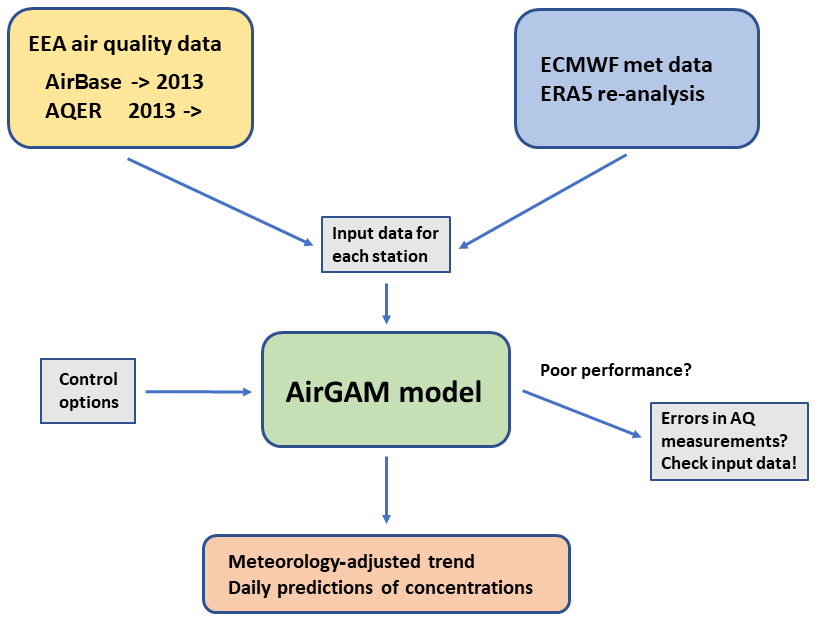
The model has been mainly developed for trend studies based on the air quality (AQ) measurement data hosted by the European Environmental Agency (EEA), including the AirBase data (before 2013) and the Air Quality e-Reporting (AQER) data from 2013 and onwards. The EEA data provide daily or hourly surface concentrations at individual monitoring stations. For the input meteorological data, we extract time series from the gridded meteorological re-analysis data (ERA5) provided by ECMWF for each monitoring station (Hersbach et al., 2018, 2020). Figure 1 shows a schematic of the data flow of AirGAM.

Figure 1 AirGAM data flow scheme.

In addition to concentrations and meteorology, the program reads several control options for the model run. Another feature of AirGAM is that it may sometimes check for errors in the air quality data. We have often found the poor performance of the model, e.g. low correlations between observed and model-predicted concentrations from cross-validation, to be associated with dubious measurement data.

AirGAM does not explicitly use emissions or background concentrations – these are sought to be implicitly represented through the estimated nonlinear relations between the concentrations and the meteorology and time variables. In addition to meteorology-adjusted trends, the program may also produce unadjusted trends – i.e. trends based on the same regression set-up but only including the time covariates. Both types of trends can be output in the same run, making it possible to compare them.

The model estimates trends over a user-defined period from a minimum of 2 years and upwards. For each year, the user may select the whole year or a sub-part of the year, e.g. only winter months (say October–March), summer months (say April–September), or any user-defined interval of months for the trend analysis. Usually, only a single set of smooth relations between the concentrations and the covariates is estimated from the data in the model. However, it is possible to operate with different groups of estimated smooth relations for different parts of the year (or sub-year) if needed, e.g. one set for the winter, say October–March, and another for the summer, say April–September. This latter capability of the model is typically necessary for modelling O₃ and PM_2.5 using data for the whole year since the relationships usually are different in the wintertime than in the summer.

1.2 Predictions in the COVID-19 year 2020

The conceptual idea behind a statistical model such as AirGAM is that the model is trained to find patterns between various input data (local temperature, wind speed, mixing height, etc.) and the daily level of pollutants (NO₂, O₃, etc.) for a given training period. Based on these patterns, the model can predict pollutant levels outside the training period. The main advantage compared to CTMs is that no assumptions on emissions are needed. Thus, the exceptional conditions experienced during the COVID-19 lockdown in 2020 offered a perfect task for such statistical models. We applied the AirGAM model for EEA's AQER data of NO₂ (EEA et al., 2020; Solberg et al., 2021b) during the first lockdown in Europe (March–July 2020) and trained the model on the data for the previous 5 years (2015–2019). The difference between the AirGAM predictions (business-as-usual results) and the observed NO₂ levels could then be related to the impact of the lockdown on mobility (road transport, aviation, etc.). Compared to gridded models such as CTMs, statistical models could be applied directly to urban stations. We found that the AirGAM model performed well for most sites while performing more poorly for a minor number of stations, which is partly explained by inconsistent measurement data. After aggregating all traffic sites (urban and suburban) for individual countries, the results showed good compliance between predicted and observed daily NO₂ levels.

The predictive capabilities of the AirGAM model come in addition to the application for long-term trend assessments. The experience from applying AirGAM specifically for a COVID-19 analysis (Solberg et al., 2021b) was that the model performed very well for NO₂ at the urban and suburban background and traffic sites. In contrast, as expected, the performance was lower at rural locations, since the NO₂ levels outside the urban areas are less determined by local meteorological conditions. The performance was lower for O₃ and PM, which is also expected, since secondary formation and long-range transport are more important processes for these compounds. Such processes are only indirectly captured by AirGAM. These results do not imply that the AirGAM model and other statistical tools are unfit for O₃ and PM assessments but rather that the model performance is somewhat lower than for a primary pollutant such as NO₂.

1.3 Outline of the paper

First, in Sect. 2, we overview the statistical GAM methodology implemented in the AirGAM model and how to interpret its trends. Section 3 gives results from a recent EEA trend study for 2005–2019, using all the available AirBase/AQER stations in Europe. Section 4 compares GAM with the RF method in the R package rmweather. In Sect. 5, we briefly discuss how AirGAM can also be used as a tool for data quality investigations. Finally, Sect. 6 contains a summary and conclusions. Appendix A lists some frequently asked questions (FAQs) regarding the model. The Supplement accompanying this paper includes a user's guide to the model describing details of its numerical implementation, all inputs to the model and how to run it on Windows and Linux, and all results files. It also contains instructions on installing the model and some run examples.

2 Model formulation

2.1 GAM models

In statistics, a GAM model (Hastie and Tibshirani, 1990; Wood, 2017) is a nonlinear regression model linking expected values μ_i of a given response variable Y_i to one or more explanatory variables x_ij through the following relations:

$$\begin{array}{}\text{(1)}& g\left({\mathit{\mu }}_i\right)={\mathit{\beta }}_{\mathrm{0}}+\sum _{j=\mathrm{1}}^p{\mathit{\beta }}_j\left(x_{ij}\right);{\mathit{\mu }}_i=E\left(Y_i\right),\end{array}$$

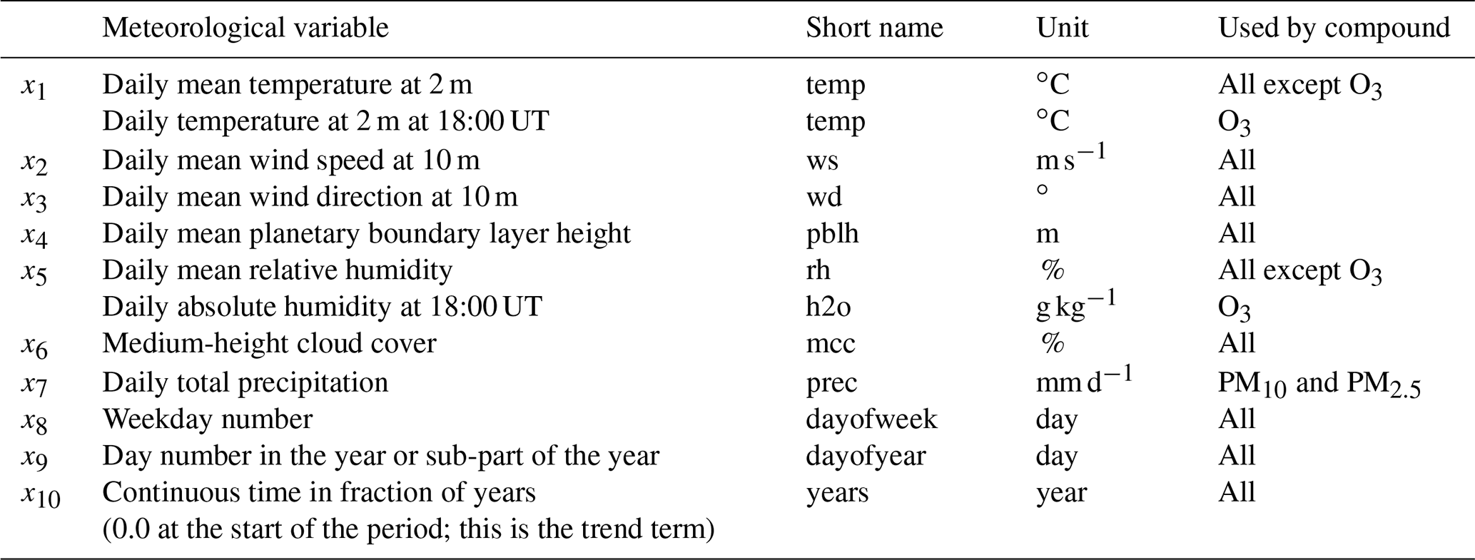
where β₀ is a constant (the intercept), and where β_j(⋅), for $j=\mathrm{1},\mathrm{\dots },p$, represents the smooth functions of the covariates x_ij, with p as the number of covariates. In our implementation of this model for air quality analysis, the response variable Y_i in Eq. (1) represents a daily average (NO₂ or PM) or maximum 8 h running mean (O₃) concentration at day number i at a given site, while x_ij represent the values of the explanatory variables, for $j=\mathrm{1},\mathrm{\dots },p$, at the same location and day. These consist of various meteorological variables such as temperature, wind, etc., and time variables such as the day of the week, day of the year, etc. The meteorological covariates depend on the air pollutant being modelled, as shown in Table 1.

In Eq. (1), g(⋅) is a function (the link function) that links the statistically expected value of the response variable Y_i, i.e. μ_i, to the covariates x_ij. Also, Y_i is assumed to have a definite probability distribution, the response distribution, with mean μ_i and variance V_i. Furthermore, in Eq. (1), each β_j is a smooth function of x_ij and not simply a constant to be multiplied with x_ij as in multiple linear regression (MLR) or generalised linear regression models (GLMs). Thus, GAM models represent an extension of these models for regression. GAMs are also more flexible than MLR models (but not GLMs), since the mean value μ_i is related to the covariates through a link function g(μ_i), which need not be the identity function g(μ)=μ.

Since the relation between air pollution and meteorology is generally nonlinear, MLR models or GLMs cannot naturally model this relationship. Only a nonlinear model, such as a GAM, capable of fitting nonlinear relations between an air pollutant and a set of meteorological covariates will have a chance of succeeding in this regard. It is then vital to choose the right set of meteorological covariates for each type of air pollutant to be modelled. Besides, various time covariates will also be needed.

Note that emissions, background concentrations, physicochemical processes, and depositions have deliberately been left out from the design of such a regression model, even though we know that air pollutants are closely linked to and primarily determined by these factors and processes in addition to meteorology. The idea is to see how far we can use meteorology and time data to model air pollutants. Limitations depend on the compound and type of data. Over the last 4 years, the current model has been developed for NO₂, O₃, PM₁₀, and PM_2.5. This development has resulted in a set of meteorological and time covariates found to model and predict concentrations of these compounds well (Table 1).

For NO₂, PM₁₀, and PM_2.5, we apply a log link g(μ)=log μ and gamma distributions as response distributions. This is because these compounds generally have a somewhat more extensive range of concentration variations than O₃, with the variance of Y_i, i.e. V_i, typically proportional to ${\mathit{\mu }}_i^{\mathrm{2}}$. For such variables, it is usual practice in GAM modelling to select a logarithmic link function and a distribution potentially skewed to the right, such as a gamma, as a response distribution for Y_i (Wood, 2017). This was also applied in the previous trend studies (Solberg et al., 2018a, b, 2019).

For O₃, we apply an identity link g(μ)=μ and normal distribution as a response distribution. This choice is because O₃ has a relatively small range of concentration variations where the variance of Y_i, i.e. V_i, does not change very much with the mean μ_i. Thus the response distribution is well represented with a symmetric distribution such as a normal.

The input variables have been selected by combining a priori knowledge of the main physicochemical processes and experience during the model development. Extensive research in previous work with the model (Solberg et al., 2018a, b, 2019) resulted in meteorological and time variables being used, as presented in Table 1. Absolute humidity is introduced as a variable for O₃ since the gas-phase reaction O^′D + H₂O → 2OH is the main production path for OH in the atmosphere and since OH, in turn, is decisive for the O₃ formation. For PM and NO₂, we used relative humidity to reflect the importance of wet deposition and cloudiness.

Table 1 List of meteorological and time variables used in the AirGAM model (Eq. 1) for various compounds. The short names refer to those used in the text and graphics files in Sect. S5 in the Supplement.

In the model, the trend term is represented as a smooth function of time (x₁₀=t) rather than a straight line, as in some previous studies (Solberg et al., 2018a, b). The main reason for this choice is for the model to be better prepared for trend studies over extended periods. In such cases, it is less relevant to represent the whole trend over the entire period as a straight line.

Since meteorological variables are included in this GAM model to explain the expected (μ_i) and observed (Y_i) concentrations of air pollutants at each time point t_i, the estimated trend β₁₀(t) in Eq. (1) will represent a so-called meteorology-adjusted trend, i.e. a trend discounting for the effects of trends or time variations in these meteorological variables over the period selected for the analysis. This represents the main output from AirGAM.

Note that none of the covariates is transformed in the model; this only applies to the concentrations of NO₂ and PM. Wind direction is the only variable which is cyclic. The day of week and day of year are not defined as cyclic variables since Sunday and Monday and 31 December and 1 January may differ considerably.

Also, wind direction and relative humidity are not provided directly in the ECMWF ERA5 data used in this study. Instead, they have been calculated from the u and v components of wind and the absolute humidity, surface temperature, and pressure found in these data. Details of this pre-processing of the ERA5 data are found in Appendix C in the Supplement.

In addition to meteorology-adjusted trends produced by the model described above, AirGAM may also estimate so-called unadjusted trends. These are trends produced by the same GAM regression model set-up as above but only including the time covariates x₈–x₁₀, i.e. removing all the meteorological covariates x₁–x₇. Both trends can be produced individually and output from the same run, making it possible to compare them. These two models will be called the meteorology-adjusted and unadjusted models in the following.

Note that, in AirGAM, we only use GAM models with covariates in a purely additive form, as shown by Eq. (1). Thus, no interactions between the variables are used, such as multiplications between variables, defining 2-dimensional smooth functions, etc. This makes the models easy to interpret, since the estimated nonlinear functions encode each independent variable's contribution to the predicted concentration. Section 4 compares our GAM models to RF models that incorporate interactions between the variables. We show that our GAM approach produces models with a predictive performance on par with this method. Thus, we argue that a purely additive model seems sufficient to build models with good predictive performance, at least for the data analysed in this paper.

2.2 Calculation of physically interpretable trend curves

AirGAM outputs trend curves as plots and data values to various result files described in Sect. S5.1.1–S5.1.2 and S5.1.9–S5.1.10 in the Supplement. To interpret a change in the trend level between two arbitrary time points in these plots and data files as a change in the expected concentration levels between the same two time points under certain well-defined conditions, it is essential to adjust the raw trend given by the estimated trend function β₁₀(t) from Eq. (1) into a physically interpretable trend curve y_trend(t).

This section describes how this is done for the various compounds and the meteorology-adjusted and unadjusted models.

First, we focus on the meteorology-adjusted model. For compounds such as O₃, where we apply an identity link g(μ)=μ in Eq. (1), the expected concentration at the time t is given by the following:

$$\begin{array}{}\text{(2)}& \mathit{\mu }\left(t\right)={\mathit{\beta }}_{\mathrm{0}}+\sum _{j=\mathrm{1}}^{p-\mathrm{1}}{\mathit{\beta }}_j\left(x_j\left(t\right)\right)+{\mathit{\beta }}_p\left(t\right)=A\left(t\right)+B\left(t\right),\end{array}$$

with $A\left(t\right)={\mathit{\beta }}_{\mathrm{0}}+{\sum }_{j=\mathrm{1}}^{p-\mathrm{1}}{\mathit{\beta }}_j\left(x_j\left(t\right)\right)$, and $B\left(t\right)={\mathit{\beta }}_p\left(t\right)={\mathit{\beta }}_{\mathrm{trend}}\left(t\right)$. Here A(t) is the contribution to the expected concentration at the time t from meteorology and the time variables for day of week and day of the year, while B(t) is the contribution to the expected concentration at the time t from the trend term. In this case, the physically interpretable trend curve is sought to be defined as the following function:

$$\begin{array}{}\text{(3)}& y_{\mathrm{trend}}\left(t\right)=A+B\left(t\right),\end{array}$$

with A determined so that a difference in trend values between two arbitrary time points, say t₁ and t₂, can be interpreted as the difference in the expected concentrations between these two time points. Thus, we need to have the following:

$$\begin{array}{}\text{(4)}& \begin{array}{rl}{y}_{\mathrm{trend}}\left(t_{\mathrm{2}}\right)-y_{\mathrm{trend}}\left(t_{\mathrm{1}}\right)& =A+B\left(t_{\mathrm{2}}\right)-(A+B\left(t_{\mathrm{1}}\right))\\ & =B\left(t_{\mathrm{2}}\right)-B\left(t_{\mathrm{1}}\right)\\ & =\mathit{\mu }\left(t_{\mathrm{2}}\right)-\mathit{\mu }\left(t_{\mathrm{1}}\right)\\ & =A\left(t_{\mathrm{2}}\right)+B\left(t_{\mathrm{2}}\right)-A\left(t_{\mathrm{1}}\right)-B\left(t_{\mathrm{1}}\right),\end{array}\end{array}$$

which holds for all values of A as long as A(t₁)=A(t₂), i.e. as long as the impact of meteorology and the two time variables is the same for the two time points. Under this assumption, Eq. (3) can be used as a physically interpretable trend curve for any value of A. However, it is natural to set A so that the trend curve values have the same time average over the period as the actual observations, i.e. ${\overline{y}}_{\mathrm{trend}}=\overline{Y}$. Then, since the smooth β_trend function from GAM always averages to zero over the time points of the trend estimation, which is a property of GAM modelling, it follows from Eq. (3) that this corresponds to setting $A=\overline{Y}$. Changes in the trend curve values can then be interpreted as changes in the expected concentrations if we assume the same impact of meteorology and day of week and day of the year for the two time points, i.e. A(t₁)=A(t₂). Note that the actual values A(t₁) and A(t₂) will usually differ.

However, notice that, with $A=\overline{Y}$, the trend curve values also correspond to expected concentrations under the average impact of meteorology and day of week and day of the year, i.e., $A=\overline{A}$. This is due to the fact that the estimated A(t) values always averages to β_o over the period of trend estimation which is estimated as $\overline{Y}$ in GAM modelling. Furthermore, the trend curve values in this case also correspond to expected concentrations under conditions in which the meteorology and day of week and day of the year smooth functions are exactly zero.

The same development as above also holds in the case of the unadjusted GAM model. There are only two time variables, i.e. day of week and day of the year, in the A(t) function in this case. Thus, Eq. (3) with $A=\overline{Y}$ can be used as a physically interpretable trend curve, where changes in the trend curve values can be interpreted as changes in the expected concentrations if we assume that A(t₁)=A(t₂), i.e. as long as the impact of, in this case, only the day of week and day of the year is the same for the two time points. Again, the trend curve values correspond to expected concentrations under the average impact of these two variables and under conditions in which their smooth functions are exactly zero.

Next, we apply the log–link function g(μ)=log μ to the more complicated GAM models for NO₂ and PM. Again, we focus first on the meteorology-adjusted model. The expected concentration level at time t is now given by the following:

$$\begin{array}{}\text{(5)}& \begin{array}{rl}\mathit{\mu }\left(t\right)& =\exp \left\{{\mathit{\beta }}_{\mathrm{0}}+\sum _{j=\mathrm{1}}^{p-\mathrm{1}}{\mathit{\beta }}_j\left(x_j\left(t\right)\right)+{\mathit{\beta }}_p\left(t\right)\right\}\\ & =A\left(t\right)B\left(t\right),\end{array}\end{array}$$

with $A\left(t\right)=\exp \left\{{\mathit{\beta }}_{\mathrm{0}}+{\sum }_{j=\mathrm{1}}^{p-\mathrm{1}}{\mathit{\beta }}_j\left(x_j\left(t\right)\right)\right\}$, and $B\left(t\right)=\exp \left\{{\mathit{\beta }}_p\left(t\right)\right\}=\exp \left\{{\mathit{\beta }}_{\mathrm{trend}}\left(t\right)\right\}$. Here again, A(t) is the contribution to the expected concentration at the time t from meteorology and the time variables day of week and day of the year, while B(t) is the contribution to the expected concentration at the time t from the trend term, for which both are given as factors in this case. Now a physically interpretable trend curve is sought defined as a function that, in this case, reads as follows:

$$\begin{array}{}\text{(6)}& y_{\mathrm{trend}}\left(t\right)=A\cdot B\left(t\right),\end{array}$$

with A determined so that again a difference in trend values between two arbitrary time points, say t₁ and t₂, can be interpreted as the difference in the expected concentrations between these two time points. Thus, we need to have the following:

$$\begin{array}{}\text{(7)}& \begin{array}{rl}{y}_{\mathrm{trend}}\left(t_{\mathrm{2}}\right)-y_{\mathrm{trend}}\left(t_{\mathrm{1}}\right)& =A\cdot B\left(t_{\mathrm{2}}\right)-A\cdot B\left(t_{\mathrm{1}}\right)\\ & =A\cdot \left(B\left(t_{\mathrm{2}}\right)-B\left(t_{\mathrm{1}}\right)\right)\\ & =\mathit{\mu }\left(t_{\mathrm{2}}\right)-\mathit{\mu }\left(t_{\mathrm{1}}\right)\\ & =A\left(t_{\mathrm{2}}\right)\cdot B\left(t_{\mathrm{2}}\right)-A\left(t_{\mathrm{1}}\right)\cdot B\left(t_{\mathrm{1}}\right),\end{array}\end{array}$$

which holds as long as $A=A\left(t_{\mathrm{1}}\right)=A\left(t_{\mathrm{2}}\right)$, i.e. as long as the impact of meteorology and the two time variables is the same for these two time points, and A is equal to this value.

Again, it is natural to set A so that the trend curve values have the same time average over the period as the actual observations, i.e. ${\overline{y}}_{\mathrm{trend}}=\overline{Y}$. Thus, $A=\overline{Y}/\overline{B}$, where $\overline{B}$ is the average of the B(t) values over the period of trend estimation (note that this latter average is a positive number due to the exponentiation in Eq. 5). Changes in the trend curve values can then be interpreted as changes in the expected concentrations if we assume this average impact of meteorology and day of week and day of the year for the two time points, i.e. $A\left(t_{\mathrm{1}}\right)=A\left(t_{\mathrm{2}}\right)=A$. Note again that the actual values A(t₁) and A(t₂) will usually differ and also differ from A.

To better understand the impact factor A in the previous paragraph, we give a formula for the expected value of this quantity. Since the conditioned observed concentrations Y_i|μ_i have expected values μ_i=μ(t_i), from Eq. (1), we have the following:

$$\begin{array}{}\text{(8)}& EA={\displaystyle \frac{E\overline{Y}}{\overline{B}}}={\displaystyle \frac{\overline{\mathit{\mu }}}{\overline{B}}}={\displaystyle \frac{\frac{\mathrm{1}}{N}\sum _{i=\mathrm{1}}^{N}A\left(t_i\right)B\left(t_i\right)}{\frac{\mathrm{1}}{N}\sum _{i=\mathrm{1}}^{N}B\left(t_i\right)}}=\sum _{i=\mathrm{1}}^N{w}_{i}A\left(t_i\right),\end{array}$$

with $w_i=B\left(t_i\right)/{\sum }_{i=\mathrm{1}}^{N}B\left(t_i\right)$. Thus, EA represents a weighted average of the A(t_i) factors with weights w_i for $i=\mathrm{1},\mathrm{\dots },N$, where N is the number of days for the trend estimation. If var(Y_i|μ_i) is uniformly bounded above, i.e. var(Y_i|μ_i)≤V for some V>0 for all i, and $\mathrm{cor}\left(Y_{i+k}\mathrm{|}{\mathit{\mu }}_{i+k},Y_i\mathrm{|}{\mathit{\mu }}_i\right)$ exponentially approaching zero as k→∞, which holds almost invariably for air quality observations, then we have from Serfling's strong law of large numbers applied to Y_i−μ_i (McFadden, 2000, chap. 4, p. 92) that $A-EA\to \mathrm{0}$ almost surely as N→∞. Thus, for large $N,A\approx EA$, and the average factor A in the trend curve will be close to a weighted average of the factors from the meteorological and time variables over the period for trend estimation given by Eq. (8), with weights based on the meteorology-adjusted B(t) values. Thus, the trend curve values correspond to expected concentrations under this weighted-average impact of the meteorological variables and variables for the day of week and day of the year.

However, the trend curve values will, in this case, not correspond to the expected concentrations under meteorology and day of week and day of the year conditions where their related smooth functions on the log scale are exactly zero. This can instead be obtained by setting $A=\exp \left({\widehat{\mathit{\beta }}}_{\mathrm{0}}\right)=A_{\mathrm{0}}$, where ${\widehat{\mathit{\beta }}}_{\mathrm{0}}$ is the estimated value of β₀ from the GAM modelling. Even though we prefer the former trend curve as output from AirGAM, since it fits better with the level of observations, the latter curve can easily be obtained by scaling the former curve with the constant $c=A_{\mathrm{0}}\overline{B}/\overline{Y}$.

The same development as above also holds in the case of the unadjusted GAM model. There are only two time variables, i.e. day of week and day of the year, in the A(t) factor function in this case. Again, for large N, A will be close to a weighted average of these factor values, as in Eq. (8), but with weights based on the unadjusted B(t) values. Thus, the trend curve values will correspond to the expected concentrations under the weighted-average impact of these two variables, or we may wish to rescale, as above, to obtain a trend curve which can be interpreted as expected concentrations under conditions in which their smooth functions on the log scale are exactly zero.

2.3 AirGAM user's guide

A user's guide to the model can be found in the Supplement to this paper. This contains a description of all input files, how to run the model on Windows and Linux, and a description and presentation of all result files. It also contains a few run examples. Furthermore, it gives details of the model's numerical implementation, including the choice of solution methods, automatic model selection, the choice of number and type of basis functions, and how uncertainties are interpreted and calculated in the trend and in the model predictions. Appendices in the Supplement contain information on downloading and installing the model for Windows and Linux and an overview of the model's warning and error messages.

Currently, the AirGAM model is developed as a single R script rather than an R library of user-callable routines. Even though having the model as a single script is less flexible than having it as a set of callable routines, we also believe our single script provides some advantages for an end-user, such as automating the sequence of steps needed to perform trend analysis for a whole or seasonal part of years for a large number of stations with automatic data checking and files automatically produced with easy identification of outcomes. The script also enables the automatic creation of model evaluation results with cross-validation analysis and model predictions for a selectable number of years. In addition, batch scripts are provided, allowing the user to perform the model runs in parallel on Windows and Linux in the case of a large number of stations. A user only needs to provide input data, define optional parameters, and run the batch scripts. This requires minimal knowledge of R and GAM modelling, since the model and the run scripts automate all the necessary steps.

The model script may also be used as an advanced starting point to develop further or from which to extract code. However, having an R library with user-callable routines based on the current script code will further the model's scope and flexible use. Thus, we might pursue developing the model also as an R library in the future.

3 Results for a European trend study 2005–2019

Here we give some results with the AirGAM model based on data from the latest EEA trend study 2005–2019 (Solberg et al., 2021a). The EEA air quality data used are based on non-aggregated time series data downloaded from https://aqportal.discomap.eea.europa.eu/index.php/users-corner/ (last access: 12 December 2022) in April 2021. Data for 2005–2012 were extracted from AirBase and for 2013–2019 as validated data (E1a) from the AQER database. The meteorological data used are based on the ECMWF ERA-5 data, which were downloaded using the Copernicus Atmosphere Monitoring Service in 2021.

Our experience from previous, similar studies (Solberg et al., 2018a, b, 2019) is that the model overall seems to perform best for NO₂, followed by O₃ and PM₁₀, and worst for PM_2.5. Section 3.1–3.4 below present results for the compounds NO₂, O₃, PM₁₀, and PM_2.5, respectively.

Seasonal conditioning was not used for model runs, i.e. use_season_cond=0. Thus, only a single set of smooth relations between the concentrations and the meteorological and time covariates was estimated and used by the model. The trend type was set to nonlinear (trend_type=nonlinear), and the number of basis functions to be used by the trend term was set to missing (k_years=NA), which implies that five basis functions (15 years$/$3) were used to represent the trend term in the model. Introducing a basis function for the trend every 3 years was considered an appropriate setting in this long-term trend study since we did not want to focus on, or model, too much of the short-term variations in the trend at individual stations but rather focus on the more main features and more long-term variations in the trend.

The bam routine in the mgcv package was always tried before the gam routine (incl_bam=1; incidentally, no gam calls were executed), and automatic model selection was turned on (incl_select=1). The AR(1) model (autoregressive model with a single, 1 d time lag) was not invoked for these runs (incl_ar1=0) to reduce the computational time, which means autocorrelation in the time series was not considered. Thus, the focus is not on accurately estimating individual uncertainties in the trend curves. In the cross-validation, the “limit covariates” approach was used to obtain robust predictions (rob_pred=limcov), i.e. covariate values outside the training interval were set to the nearest value in this interval before being used in the predictions. For all compounds except for O₃, all months in each year were used to estimate the trend (subyear=jan-dec). For O₃, only the summer period (April–September) was used for a summer trend study (subyear=apr-sep).

3.1 NO₂

For NO₂, there are 1485 stations in the AirBase/AQER database for 2005–2019 that fulfil the data coverage criteria for this compound (75 % coverage for individual years and 75 % coverage of years in the period), excluding the industrial stations. This forms the basis for the trend study for this compound. Due to the large number of stations for NO₂, we refrain from showing any individual station results here. Input data and results for all stations for this compound can be found in the model's data repository (Walker and Solberg, 2022b–c).

However, the results for station EE0018Ah (Õismäe) are shown in Sect. S5 in the Supplement, which describes the output results from the AirGAM model. This is a background station in an urban part of Tallinn, Estonia, with coordinates 52.41417^∘ N and 24.64946^∘ E, at 6 m a.s.l. (above sea level). This station was chosen to illustrate the results, since it is the exact median station of all stations based on the cross-validation correlation results for NO₂. Thus, it is neither the best nor the worst station but may be viewed as typical of the results for this compound. In the Supplement, Fig. S2 shows the primary trend results in a meteorology-adjusted trend for 2005–2019. Figure S3 shows plots of all smooth functions of meteorology and time-explanatory variables based on all training data for the same period. A plot of model predictions from the cross-validation for 2019 based on data for the left-out years of 2005–2018 is presented in Fig. S4. Figures S5–S8 show plots of observed and predicted annual and monthly average concentrations with trend curves and yearly and monthly median concentrations. Furthermore, for this station, you may also find plots of all evaluation results in the Supplement in the individual sub-sections of Sect. S5.2–S5.3. All results are commented upon there in the respective sub-sections of Sect. S5.1–S5.3.

3.1.1 Results for all stations

Figure 2 shows a panel of three maps of stations over Europe. The maps are made for the following three categories of stations: (1) background stations in rural areas (left), (2) background stations in urban/suburban areas (middle), and (3) traffic stations in any area (right). In each map, we present the percentage change in expected concentrations of NO₂ from 2005 to 2019, relative to the initial levels in 2005, based on the estimated meteorology-adjusted trend for NO₂ for each station. The stations plotted in each map are the stations for which the 2005–2019 cross-validation gave a correlation between observed and model-predicted values above 0.65. This resulted in 205, 742, and 409 stations, respectively, for the three types of stations, with 1356 in total.

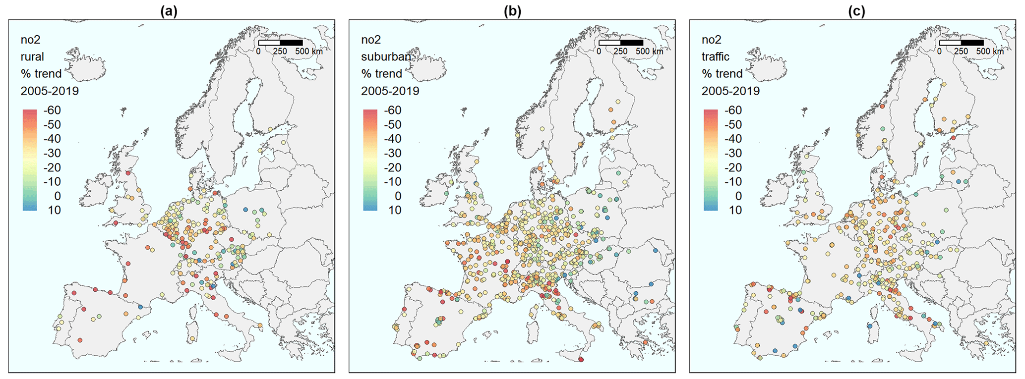
Figure 2 Maps of stations in Europe with the percentage change in expected concentrations from 2005 to 2019, relative to the initial level in 2005, based on the meteorology-adjusted trend for NO₂. (a) Background stations in rural areas. (b) Background stations in urban/suburban areas. (c) Traffic stations.

For each station, the change in the expected concentration level is calculated based on the physically interpretable trend curves y_trend(t) as output from the model at the two time points, t₁ and t₁, corresponding to the start and end of the trend estimation period 2005–2019, respectively (i.e. 1 January 2005 and 31 December 2019). Thus, the absolute change in the expected concentration is calculated as y_trend(t₂)−y_trend(t₁), while the relative percent change is calculated as $\mathrm{100}\times \left(y_{\mathrm{trend}}\left(t_{\mathrm{2}}\right)-y_{\mathrm{trend}}\left(t_{\mathrm{1}}\right)\right)/y_{\mathrm{trend}}\left(t_{\mathrm{1}}\right)$. Section 2.2 describes how the trend curves are interpreted and calculated based on the output from the GAM model.

The maps indicate a weak west-to-east gradient, with more substantial declines in the west and smaller in the east. This is particularly marked for the urban/suburban background stations (middle panel), with the densest geographical coverage. The result is mixed with countries showing both substantial reductions and sites with no trend or even increasing levels for traffic sites. This reflects that the roadside stations are more heterogeneous and subject to changes in the local urban environment (roads, buildings, etc.). Additionally, the NO₂ $/$ NO_x ratio in tailpipe emissions will strongly influence these sites, depending on the fleet of vehicles (fraction of diesel cars) and the ambient ozone level. These issues will be reduced and smoothed out for background stations due to atmospheric mixing and the NO₂ $/$ NO_x concentration ratio approaching the photo-stationary steady state determined by solar radiation, temperature, and ozone level.

Figure 3 shows box plots of the same changes in expected concentrations for the same three categories of stations. The three left plots show the relative change in percent as in Fig. 2, while the three right plots show the absolute changes in concentration levels.

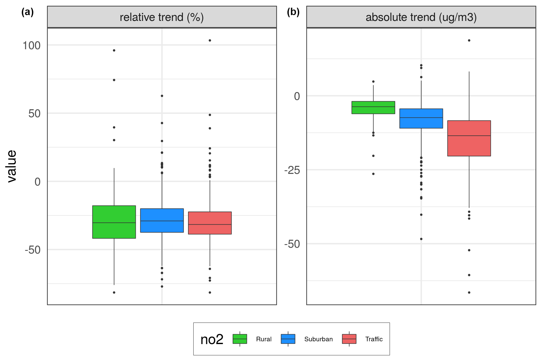
Figure 3 Box plots of changes in expected concentrations over the same three types of stations as in the map plots in Fig. 2. Panel (a) shows relative percent changes, while panel (b) shows absolute changes from 2005 to 2019 (units in % and µg m⁻³).

The results in Fig. 3 show that the NO₂ concentration has decreased approximately at the same rate at all station categories during 2005–2019. Median reductions of 29 % are found for the rural and urban/suburban stations and 31 % for the traffic stations, with corresponding decreases in concentrations of 4–13 µg m⁻³.

Figure 4 shows box plots of some selected statistical evaluation parameters based on the cross-validation for 2005–2019. Again, the box plots are made for the same three categories of stations as in Figs. 2–3.

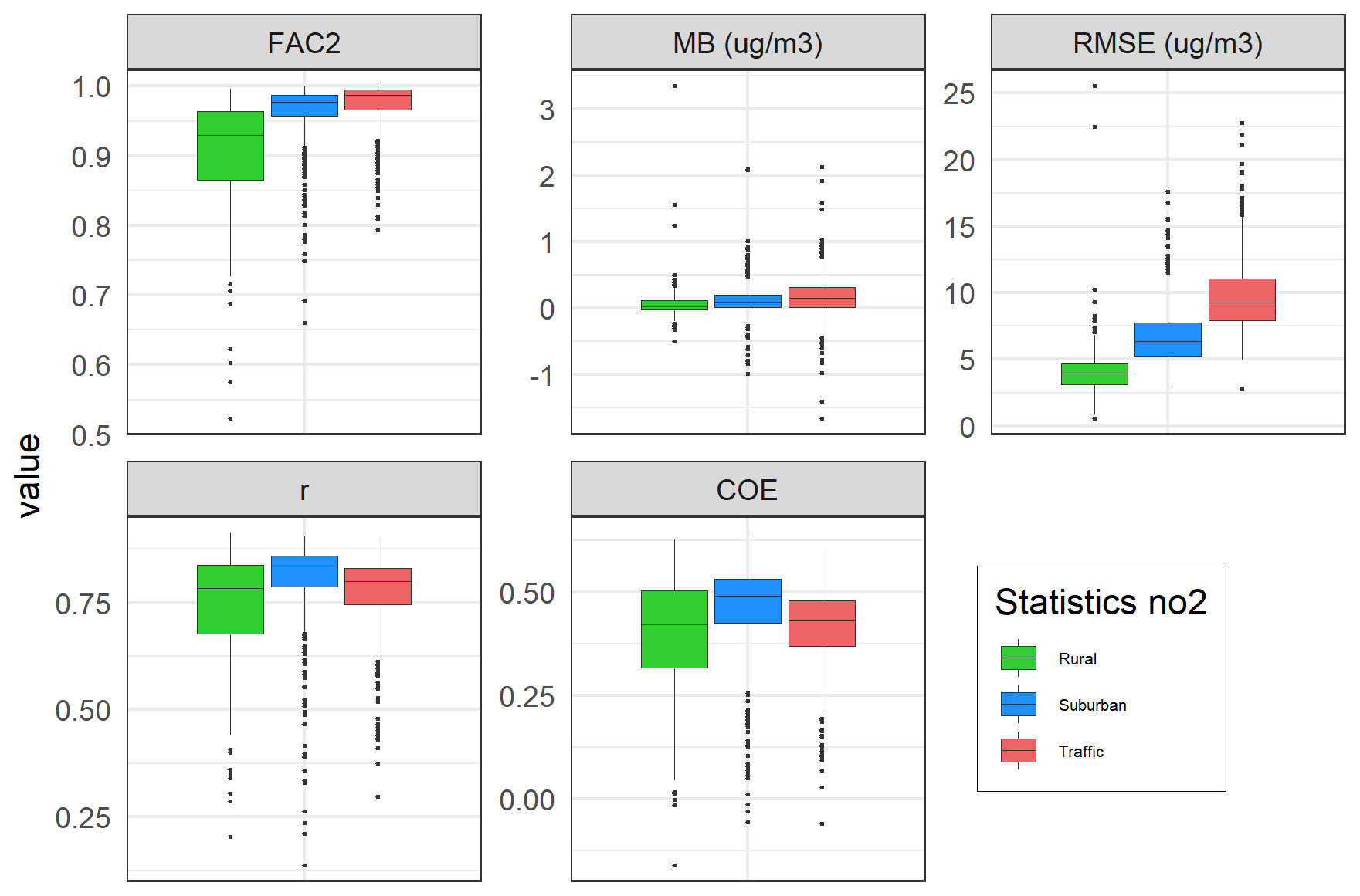
Figure 4 Box plots of some selected evaluation parameters from the cross-validation for 2005–2019, again for the same three categories of stations as in Figs. 2–3.

The statistical evaluation parameters are calculated in AirGAM using the routine modStats from the openair package in R. The manual pages for the modStats routine contain a detailed description of what these parameters represent and how they are calculated (see also Sect. S5.2.4 in the Supplement).

As seen from Fig. 4, the predictive performance of the AirGAM model for NO₂ concerning the correlation (r) and coefficient of efficiency (COE) is somewhat better for the urban/suburban background stations than for the traffic and rural ones. However, the median values of r and COE are pretty decent for all three types. Regarding FAC2 (fraction of days with predictions within a factor of 2 of observations) and RMSE (root mean squared error), traffic and rural sites are best, respectively, and hence, we have a somewhat mixed picture from these sites. Nevertheless, FAC2, r, and COE are slightly poorer, i.e. lower, for rural stations, which is expected, since the NO₂ levels at these sites depend less on the local meteorological conditions than suburban and urban sites. Also, note that the mean bias (MB) is close to zero for all three types of stations, which is good.

3.2 O₃

For O₃, there are 1175 non-industrial stations in the AirBase/AQER database for 2005–2019, fulfilling the data coverage criteria for this compound (75 % coverage for individual years and 75 % coverage of years in the period). For this compound, the air quality data consist of maximum daily running 8 h average (MDA8) concentrations for each day. Again, no individual station results are shown here, but all data and results for this compound for all stations can be found in the model's data repository (Walker and Solberg, 2022b, d). Figures 5–7 show the same type of results as for NO₂.

The stations plotted in each map in Fig. 5 and as data values in Fig. 6 are the stations for which the 2005–2019 cross-validation for O₃ gave a correlation above 0.65. This resulted in 303, 594, and 44 stations, respectively, for the three types of stations, with 941 in total. However, for the evaluation in Fig. 7, all 1175 stations are used, with 368, 729, and 78 in each category.

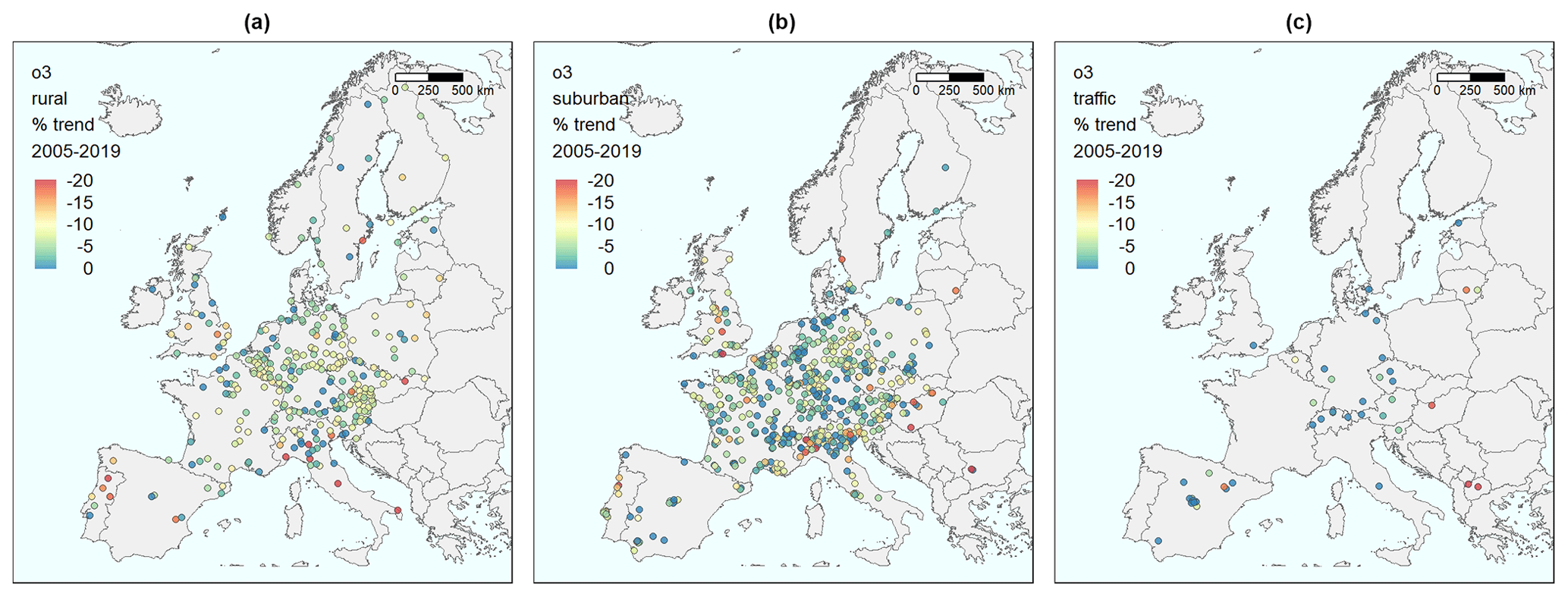
Figure 5 Maps of stations in Europe with the percentage change in expected concentrations from 2005 to 2019, relative to the initial level in 2005, based on the meteorology-adjusted trend for O₃. (a) Background stations in rural areas. (b) Background stations in urban/suburban areas. (c) Traffic stations.

The geographical distribution of the ozone summertime changes in mean MDA8 shows no clear pattern (Fig. 5). The rural stations offer reductions (yellow–green colours) over most areas, with more substantial decreases at some stations, which are mainly in Portugal and Italy. The changes at urban/suburban sites are closer to zero at many locations, but several stations also show marked reductions.

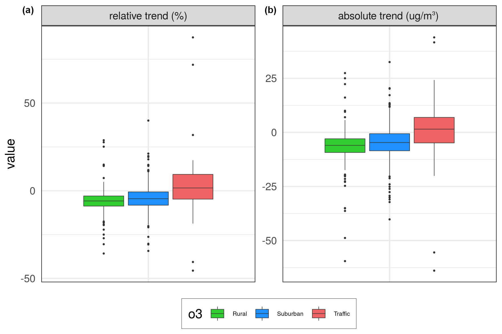
Figure 6 Box plots of changes in expected concentrations over the same three types of stations as in the map plots in Fig. 5. Panel (a) shows relative percent changes, while panel (b) shows absolute changes from 2005 to 2019 (units in % and µg m⁻³).

As shown in Fig. 6, the calculated changes in the mean summer half-year of MDA8 during 2005–2019 are substantially smaller than the changes found for NO₂ over the same period. For the rural and urban/suburban stations, a median reduction of 6 % and 5 % is found, respectively, while a slight increase of 2 % is seen for the traffic sites. The corresponding changes in concentrations are from −6 to 2 µg m⁻³ from 2005 to 2019.

Figure 7 Box plots of evaluation parameters from the cross-validation for 2005–2019 (again for the same three types of stations).

Otherwise, the results for ozone (Fig. 7) show the opposite compared to NO₂ regarding model performance. The best performance (high FAC2, r, and COE) is seen at rural stations and the poorest at traffic sites. However, the model performance for the urban/suburban category is very close to the rural one.

3.3 PM₁₀

For PM₁₀, there are 1243 non-industrial stations in the AirBase/AQER database for 2005–2019, fulfilling the data coverage criteria for this compound (75 % coverage for individual years and 65 % coverage of years in the period). No individual stations are shown, but all data and results can be found in the model's data repository (Walker and Solberg, 2022b, e).

Figures 8–10 show the same type of results as for the previous compounds. The stations plotted in each map in Fig. 8 and as data values in Fig. 9 are the stations for which the 2005–2019 cross-validation for PM₁₀ gave a correlation above 0.55. This resulted in 176, 627, and 351 stations, respectively, for the three types of stations, with 1154 in total. For the evaluation in Fig. 10, all 1243 stations are used, with 204, 658, and 381 in each category.

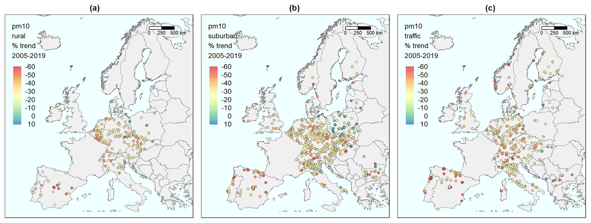
Figure 8 Maps of stations in Europe with the percentage change in expected concentrations from 2005 to 2019, relative to the initial level in 2005, based on the meteorology-adjusted trend for PM₁₀. (a) Background stations in rural areas. (b) Background stations in urban/suburban areas. (c) Traffic stations.

For PM₁₀, AirGAM estimates marked reductions during 2005–2019 with indications of a west-to-east gradient (Fig. 8), as was found for NO₂. Median decreases of 31 % are found for the rural and urban/suburban stations and 37 % for the traffic stations (Fig. 9), with corresponding reductions in concentrations of 7–13 µg m⁻³. Many Polish and Baltic sites have no change or even increased levels. Due to the shift from daily based sampling to hourly in France, no trends could be calculated for sites there.

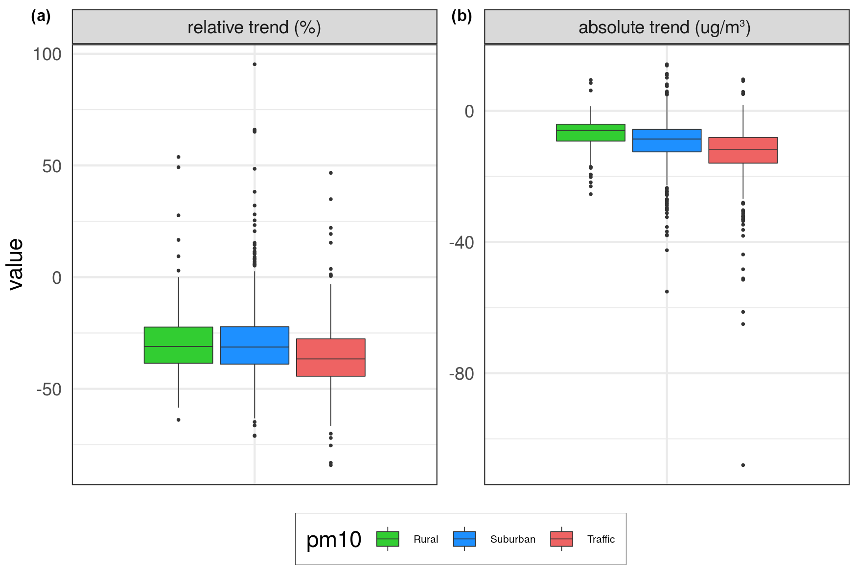
Figure 9 Box plots of changes in expected concentrations over the same three types of stations as in the map plots in Fig. 8. Panel (a) shows relative percent changes, while panel (b) shows absolute changes from 2005 to 2019 (units in % and µg m⁻³).

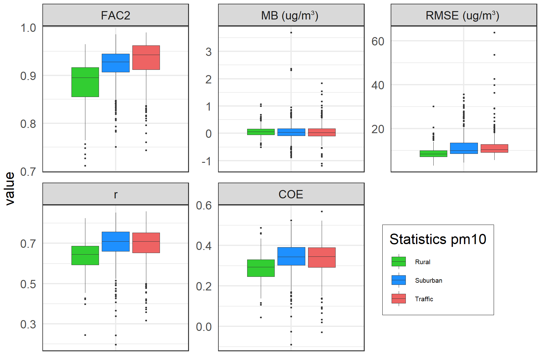
Figure 10 Box plots of evaluation parameters from the cross-validation for 2005–2019 (again for the same three types of stations).

The AirGAM performance is best at the traffic and urban/suburban sites, with slightly poorer results for the rural ones (Fig. 10). This is as expected for PM₁₀ (as for NO₂), mainly due to these stations being exposed to more direct local emissions. In contrast, the PM₁₀ at rural sites is more influenced by long-range air mass transport and external processes not captured so well by the AirGAM model, such as windblown dust, forest fires, agricultural fires, etc.

3.4 PM_2.5

For PM_2.5, there are 354 non-industrial stations in the AirBase/AQER database for 2005–2019, fulfilling the data coverage criteria for this compound (75 % coverage for individual years and 65 % coverage of years in the period). No individual stations are shown, but all data and results can be found in the model's data repository (Walker and Solberg, 2022b, f).

Figures 11–13 show the same type of results as for the previous compounds. The stations plotted in each map in Fig. 11 and as data values in Fig. 12 are the stations for which the 2005–2019 cross-validation for PM_2.5 gave a correlation above 0.55. This resulted in 59, 186, and 80 stations, respectively, for the three types of stations, with 325 in total. For the evaluation in Fig. 13, all 354 stations are used, with 67, 201, and 86 in each category.

Figure 11 Maps of stations in Europe with the percentage change in expected concentrations from 2005 to 2019, relative to the initial level in 2005, based on the meteorology-adjusted trend for PM_2.5. (a) Background stations in rural areas. (b) Background stations in urban/suburban areas. (c) Traffic stations.

The number of stations for PM_2.5 is substantially lower than for the other compounds, and thus the interpretation of the results becomes more uncertain. However, the sites with sufficient monitoring length showed a marked reduction in the expected concentration level (with a few exceptions) during 2005–2019 (Fig. 11). The geographical coverage is too sparse to conclude the spatial pattern in the trends. As a median over the sites, we find relative reductions of 28 %, 31 %, and 37 % at rural, urban/suburban, and traffic sites, respectively (Fig. 12), with corresponding reductions in the concentration of 4–7 µg m⁻³.

Figure 12 Box plots of changes in expected concentrations over the same three types of stations as in the map plots in Fig. 11. Panel (a) shows relative percent changes, while panel (b) shows absolute changes from 2005 to 2019 (units in % and µg m⁻³).

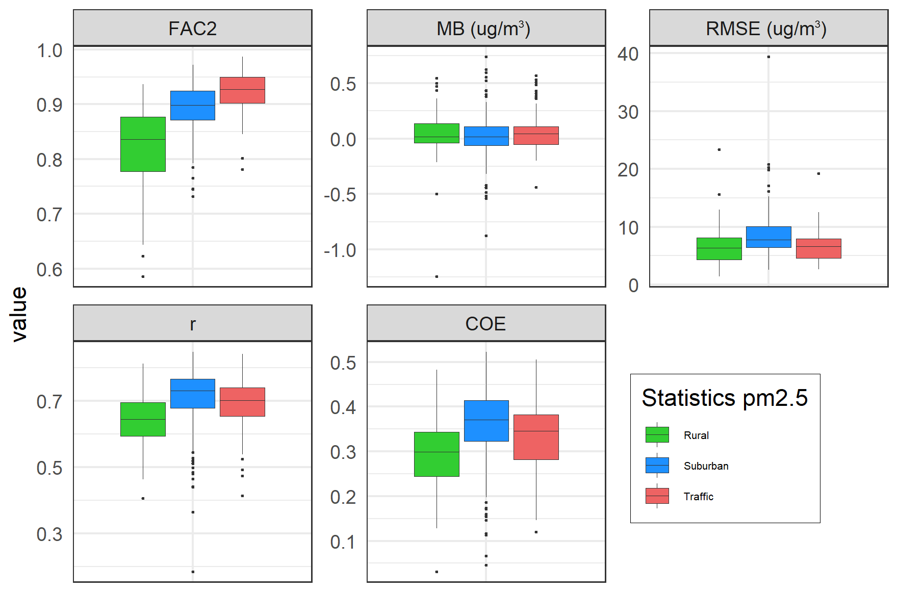
Figure 13 Box plots of evaluation parameters from the cross-validation for 2005–2019 (again for the same three types of stations).

The AirGAM performance is best at the traffic stations concerning FAC2 but nearly the same for MB and RMSE (Fig. 13). For correlation r and COE, the urban/suburban and traffic stations are slightly better than the rural ones.

4 Comparison with the random forest method in rmweather

Another approach for discounting the effect of meteorology when estimating trends in air quality data is the random forest (RF) method (Ho, 1995; Breiman, 2001) as implemented, e.g., in the R package rmweather (Grange et al., 2018; Grange and Carslaw, 2019). We will briefly describe the main similarities and differences between GAM and RF and then compare them using the data from the present trend study.

Both methods attempt to solve a nonlinear regression with concentrations as a response and a given set of meteorological and time variables as covariates. However, the nature of their solution methods is quite different. In GAM, we estimate a set of nonlinear relations between the response and the covariates by regularisation, i.e. by maximising a penalised likelihood. This produces smooth and non-wiggly estimated relations between the response and each covariate, resulting in a model that avoids overfitting and generalises well to new data not in the training set.

The RF approach uses decision trees as its main building block for relating the response to the covariates. Several datasets are then created randomly by bootstrapping, i.e. random sampling of new data with replacements from the available data, including randomly selecting various subsets of the available covariates. Then decision trees are fitted individually to these data. Finally, an ensemble of such fitted trees defines the nonlinear relations and predictions. The latter are produced as mean values over the predictions from individual trees in the forest. This results in a model that avoids overfitting and generalises well to new data. Although they cannot be classified as robust methods per se, GAM and RF are not very sensitive to outliers. They can also handle missing data well.

Both methods result in interpretable models. We can quickly inspect the estimated nonlinear relations between the response and each covariate to see if an association makes physical sense. In GAM, for this purpose, we use the set of estimated smooth functions, including the smooth function for the trend, while in RF, we use a similar set of so-called estimated partial dependencies. In the latter method, a trend is estimated by calculating meteorologically normalised concentrations over time, i.e. mean concentrations predicted from the RF model using average meteorology. In GAM, uncertainties in the smooth functions are output directly as a byproduct of the estimation. For RF, however, bootstrapping, using randomly sampled data and repeated estimations, must generally be used to estimate uncertainties in the partial dependencies and the meteorologically normalised concentrations.

A nice feature of the RF approach is that concurvity or collinearity between the covariates is handled efficiently and is thus not an essential issue for these models, while this can be detrimental for GAM models and needs to be checked. However, our experience in the present study shows this to be a pretty minor issue, with only a few cases of potential problems, despite many stations. RF also has model selection built-in, since the method will ignore a variable not contributing to predicting a response. GAM also has model selection built-in when we turn on the select=TRUE option in the calls to the bam and gam routines.

Also, more assumptions are built into a GAM model relative to an RF model. For example, in GAM, we need to assume a specific probability distribution for the response given the covariates, and we need to consider the transformations of the former. In contrast, no distributions or transformations must be specified in an RF. Furthermore, GAM assumes a smooth and continuous underlying relation between the response and each covariate. In our case, smooth and continuous relations are often found between air pollution and related meteorological and time variables. However, such smooth and continuous relations are not considered in an RF approach, and they can be non-smooth and discontinuous. Even if perhaps not directly discontinuous, more abrupt changes in the trend, for example, may happen if policy changes or mitigation measures lead to changes in emissions and subsequent concentration levels at a station over a relatively short period. Such sharp transitions will typically be more smoothed out in a GAM model unless we use a higher number of basis functions around the time of the events.

A trend analysis based on hourly values of NO₂ for the traffic station GB0682Ah – Marylebone Road, London – for 1997–2016 was conducted in Grange and Carslaw (2019) using the RF method in rmweather. Their paper focuses on the impact on the trend due to various interventions imposed on road traffic in London during this period. These interventions aim to reduce primary NO₂ emissions from vehicles, leading to lower NO₂ concentrations. To compare AirGAM with RF, we have applied a similar trend analysis here for this station for 2005–2019, using daily mean values of NO₂ as input rather than hourly data. In our study, we use the same meteorological and time variables in RF as in AirGAM, i.e. we use meteorology from ECMWF ERA5 for this station rather than data from Heathrow Airport, which was used in their paper. The meteorological covariates are the same in both studies, except for planetary boundary layer height and cloud cover, which is used here for both models, and atmospheric pressure, which is not used. Otherwise, we run with the same hyperparameters in RF as in their paper, using 300 trees in the forest, a minimal node size of five, and the default number of variables split at each node, which is three in our case. The seed number in the calls to the routines in rmweather was set to 1234. A default of 300 predictions was used to produce the meteorologically normalised concentrations.

As for AirGAM, we run with the same set-up as for the other runs in this paper, but we introduce a somewhat more agile GAM model by increasing the number of basis functions for the trend from the default of 5 to 10. This is the smallest number of basis functions considered to be sufficient, according to the gam.check routine (k−1 − edf > 0.5), thus introducing just the right amount of model complexity for the trend in GAM for this more detailed trend analysis. We also consider auto-correlation in the time series by including an AR(1) model for the model residuals using the option incl_ar1=1 in AirGAM.

Figure 14 shows the meteorologically normalised trend from the RF model (blue curve) as monthly averages and the meteorology-adjusted smooth trend from AirGAM (dark green curve) for NO₂ at Marylebone Road, London, for 2005–2019. In the figure, the dark green dashed curves form a 95 % confidence region for the trend from AirGAM.

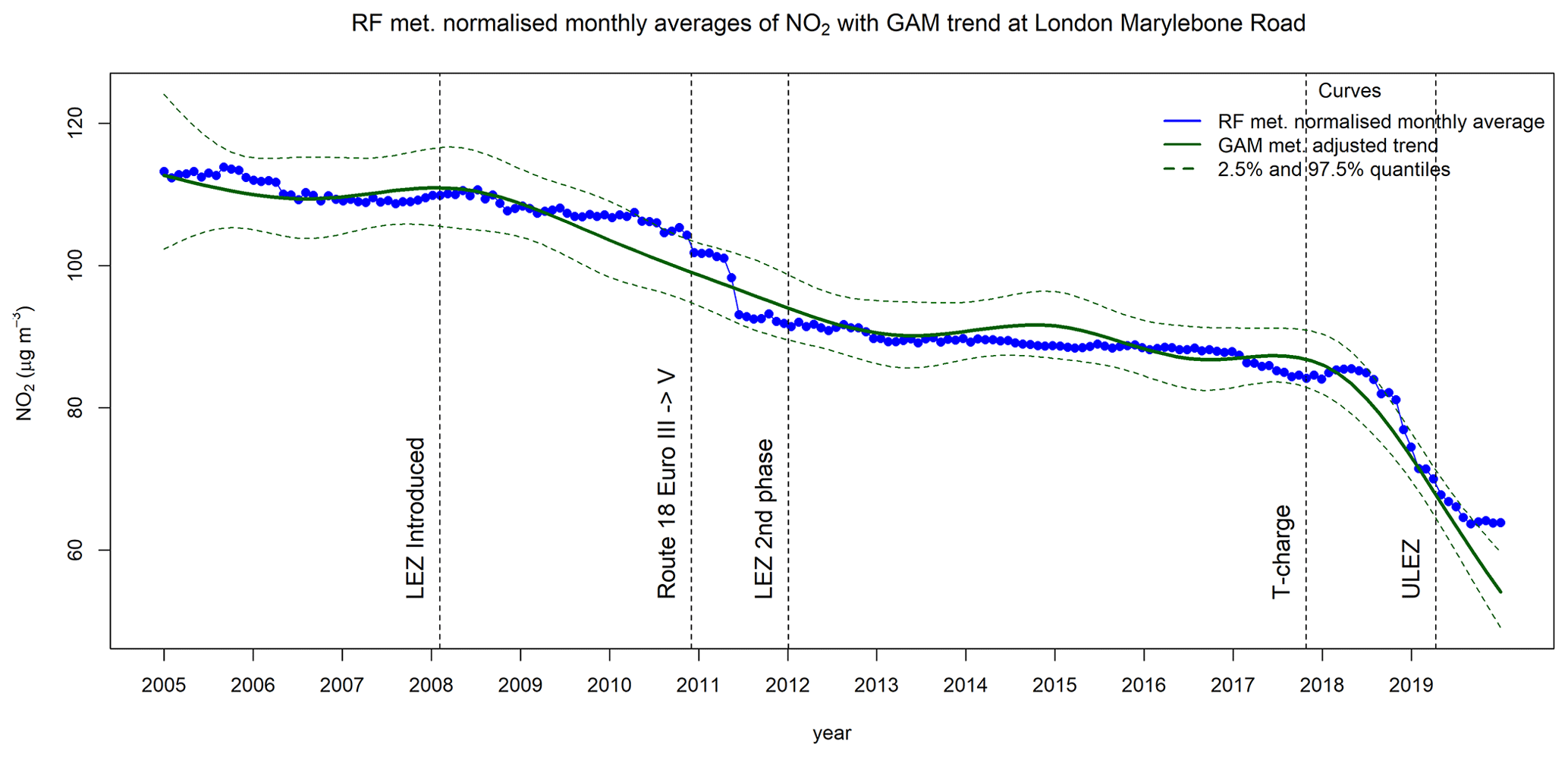
Figure 14 Meteorologically normalised trend (monthly averages) from the RF model (blue curve) together with a meteorology-adjusted smooth trend (dark green curve) from AirGAM with a 95 % confidence region (dashed curves) for NO₂ at Marylebone Road, London, for 2005–2019 (units in % and µg m⁻³).

The vertical dashed lines in the figure show air quality interventions in London during this period. The first two highlighted in Grange and Carslaw (2019) are identified as breakpoints from a time series breakpoint detection analysis conducted there. These are associated with the introduction of the Low Emission Zone (LEZ) in London on 4 April 2008 and the change from Euro III to Euro V vehicles on Route 18 at the end of 2010. The following two interventions (second phase of LEZ on 3 January 2012 and the introduction of the toxicity surcharge (T-charge) on 23 October 2017 were also considered in their paper but not identified as actual breakpoints for the trends in their analysis. The last intervention shown in the figure introduces the Ultra Low Emission Zone (ULEZ) in London on 4 April 2019. For a more thorough description of these interventions, see Grange and Carslaw (2019). A detailed description of the history and development of various congestion charges introduced in London to curb the levels of air pollution from the mid-1990s to the present is given in Wikipedia (2022).

As shown in Fig. 14, the shape of the trend curve from the GAM model resembles the trend point values from the RF model with some noticeable differences. The GAM curve is smooth and not too wiggly by construction, falling gently in several phases with more flat in-between parts before decreasing sharply at the end from around the introduction of the T-charge in 2017 and towards 2020. The concentration level is reduced from 113 µg m⁻³ in 2005 to 54 µg m⁻³ in 2020, with a total reduction of 59 µg m⁻³. The trend values from RF are more variable, presumably due to the more adept nature of this method. Here the level is reduced from 113 µg m⁻³ in 2005 to 64 µg m⁻³ in 2020, with a total of 49 µg m⁻³ that is 10 µg m⁻³ less than for GAM, mainly due to the differences in the trends at the very end of the period. Also noticeable is the sharp decrease in the RF trend around the time of the Route 18 bus fuel changes from late 2010 to the middle of 2011, which the GAM model does not reproduce. Instead, GAM estimates a smooth and gentle reduction in the concentrations over a much more extended period from just after the introduction of the LEZ in 2008 to the middle of 2013.

Note that, despite differences in the shapes of these trend curves, the RF trend is well contained within the 95 % confidence region for the GAM trend, except for 5 months in 2010–2011 and 6 months at the end of the period, which is a total of 11 months. If the RF point values were the true trend, then we would expect around nine monthly values (5 % of 180 months) outside this interval. However, they are also estimated and not identical to the true trend. It is challenging to state the most realistic trend – is it the smooth and non-wiggly trend from GAM or the more variable and detailed trend from RF? The sharp declines in the RF trend around the introduction of the Route 18 bus fuel changes may well indicate that the RF trend in this period is the most realistic. On the other hand, the gentle reduction in the GAM trend from the LEZ introduction in 2008 towards 2011, a period where the RF trend is more constant, is also interesting and may point to cuts in NO₂ emissions from traffic affecting the station in this period. Thus, it may be beneficial to use both methods in more detailed trend analyses to obtain a more diverse picture of and insight into the possible nature of the actual trend.

Comparing the trends produced from AirGAM and the RF method in rmweather for other stations and compounds (not shown here) gives, in most cases, the same picture as above. The GAM approach in AirGAM produces trend curves that are smooth and non-wiggly, while the RF approach tends to create more variable trends with more details. All in all, however, we found the trends to be similar in most cases. It would be interesting to study how well the two methods estimate trends using controlled experiments with simulated but realistic data to know the underlying trend. We hope to pursue such a study in a forthcoming paper.

Table 2 shows, for the various compounds, the prediction accuracy of the GAM models in AirGAM versus the RF method in rmweather from the cross-validation for 2005–2019. Here, the evaluation parameters, i.e. prediction performance metrics, are the same as those used in Sect. 3. Each metric in the table is calculated as a mean over the n individual stations for each compound. The corresponding number in parentheses is an estimated standard deviation of this mean value obtained from bootstrapping using 5000 replications of the individual values in each case.

Table 2 Prediction accuracy from the cross-validation for 2005–2019 of AirGAM vs. RF from rmweather. The prediction performance metrics are the same as those used in Sect. 3. Values in bold mark the best-performing model for each compound and metric. Note: SD is the standard deviation.

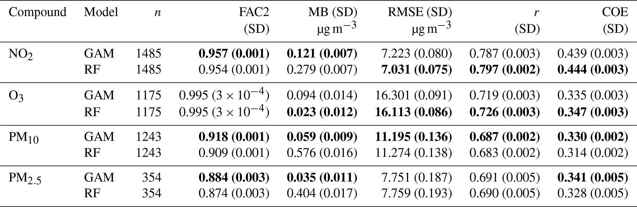
As shown in Table 2, the two methods are similar in the predictive performance concerning the various evaluation parameters shown. For some compounds and performance metrics, GAM is best; for others, RF is best, but the difference between the two is slight, except perhaps for the mean bias (MB), where GAM is clearly better than RF for all compounds except for O₃, where RF is slightly better. Bootstrapping the differences in the metrics between the models results in the bold values in the table, where one model is statistically significantly better than the other at the 1 % level. In terms of the concentration level independent metrics correlation (r) and coefficient of efficiency (COE), both models seem to perform best for NO₂, followed by O₃ and then PM, although GAM is fairly good regarding COE for PM_2.5. Overall, both methods perform pretty well for all metrics shown, but GAM seems to have an edge in PM, while the opposite is true for NO₂ and O₃.

Interaction between covariates means that a covariate's influence on the response depends on the level of one or more of the other covariates. RF models, such as those produced by rmweather, can potentially include complex interactions between the covariates. Strictly additive GAM models used by AirGAM do not have any interactions between covariates. Since they are very similar in predictive performance for all compounds in this comprehensive trend study, there seem to be few or no interactions between the covariates that need to be modelled to obtain a good predictive performance, at least for these data. Thus, a purely additive model with no interactions appears to be sufficient.

5 AirGAM as a tool for data quality investigations

A spin-off of the AirGAM model is the ability to detect measurement data of dubious quality. This is easily explained, as AirGAM is based on finding long-term systematic relationships between reported levels of air pollutants and meteorological and temporal data. When this approach fails, it is either due to the station being dominated by long-range transport of air pollutants (whereas AirGAM relies on local meteorological data) or a result of artefacts in the monitoring data, such as significant shifts in the concentration level or the seasonal cycle or other kinds of spurious effects. As described in previous reports (Solberg et al., 2018a, b), screening the AirGAM results on the lowest correlation coefficients (and high values for NMGE, the normalised mean gross error) has proven to be a valuable tool for detecting errors in the measurement data. Solberg et al. (2018a, b) give various examples of time series of dubious quality identified by screening the AirGAM results. The examples include time series with a substantial offset in specific years and ozone data given in a faulty unit (parts per billion vs. µg m⁻³) during parts of the period. Although such errors could have been identified with basic statistical tools, other types of artefacts would have been harder to detect. This includes time series of PM₁₀ at certain stations and years that turned out to be displaced by 1 d. AirGAM predicted the daily concentrations fairly accurately for these time series, whereas a systematic shift of 1 d was seen compared to the observational time series. Further investigations confirmed that the timestamp of the measurements was indeed wrong. This type of error in the monitoring data would have been tough to detect by more basic statistical methods.

6 Summary and conclusions

This paper presents the AirGAM model – an air quality trend and prediction model developed at NILU in cooperation with EEA over the years 2017–2021. The model is based on solving a nonlinear regression using generalised additive modelling (GAM) of daily observed concentrations at individual air quality monitoring stations with corresponding meteorological and time-related explanatory variables. It has been developed primarily for NO₂, O₃, PM₁₀, and PM_2.5. Since the concentrations are conditioned on local meteorology in the regression, the trend estimated by the model may be viewed as a meteorology-adjusted trend – i.e. a trend in concentrations discounting for the effects of time variations and trends in the meteorological data. The model can also produce unadjusted trends, i.e. trends using the same regression set-up but only including the time variables. These can then be compared with the meteorology-adjusted trends to see the effect of the meteorological adjustment. Unadjusted trends show changes in actual concentrations with time. In contrast, meteorology-adjusted trends show changes in concentrations mainly due to changes in emissions or physicochemical processes not induced by meteorology.

The meteorological and time covariates used in AirGAM have been carefully selected on physical grounds for each pollutant as part of the model development. Generally, they were statistically significant both in our earlier studies and in our present study involving EEA AirBase/AQER stations in Europe for 2005–2019. Thus, we believe that they are reasonable explanatory variables for the concentration variations. However, performing model selection is vital as good practice in statistical regression with many covariates. Due to the large number of stations to be handled, more traditional model selection techniques of including or excluding individual covariates in a step-wise fashion were found to be intractable to implement in the model. Instead, a form of automatic model selection is introduced via extra penalisation in the GAM solver routines, forcing any non-essential or superfluous covariate to be pushed towards a zero-flat function and thus removed from the regression. Based on this in our present study, most covariates were significant at the 5 % level, with only a few non-significant at some stations (mostly cloud cover for NO₂ and precipitation for PM).

A concurvity analysis performed in the present study shows all covariates to be relatively independent of each other for all compounds, with concurvity values of type estimate for the most part below 0.4. Higher values occurred only in 0.55 %, 0.09 %, 0.31 %, and 0.53 % of the cases (stations and covariates) for NO₂, O₃, PM₁₀, and PM_2.5, respectively. For NO₂ and PM, all values were below 0.5, while, for O₃, only three were in the interval [0.5, 0.6]. This generally indicates good statistical identifiability of the model variables, implying a reasonable estimation of the smooth nonlinear relations, including the trend. In AirGAM, as a default, a basis function is introduced in the trend term every 3 years with data, which typically estimates the trend's main features and long-term properties quite well in most cases. However, the user may choose a higher number of basis functions for the trend if it is essential to capture more details and short-term variations.

Our present trend analysis in Europe for 2005–2019 shows that the NO₂ concentration has decreased approximately at the same rate at all station categories during this period. Median reductions of 29 % are found for rural and urban/suburban stations and 31 % for traffic stations, with corresponding decreases in concentration levels of 4–13 µg m⁻³. For O₃ at the rural and urban/suburban stations, median reductions of 6 % and 5 % are found, respectively, while a slight increase of 2 % is seen for the traffic sites. Corresponding changes in concentrations are from −6 to 2 µg m⁻³. For PM₁₀, median reductions of 31 % are found for the rural and urban/suburban stations and 37 % for the traffic stations, with corresponding decreases in concentrations of 7–13 µg m⁻³. And, finally, for PM_2.5, we find median reductions of 28 %, 31 %, and 37 % at rural, urban/suburban, and traffic sites, respectively, with corresponding decreases in concentrations of 4–7 µg m⁻³. Thus, these are our estimated changes in concentration levels due to changes in emissions or physicochemical processes and not due to meteorology during this period.

Cross-validation at the stations in Europe for 2005–2019 shows that the model works well and can predict concentrations with reasonably good accuracy in this period for most stations, with correlations ranging from 0.69 for PM to 0.79 for NO₂ and RMSE ranging from 7.2 µg m⁻³ for NO₂ to 16.3 µg m⁻³ for O₃. Comparison with other approaches for estimating meteorology-adjusted trends based on nonlinear regression, such as the random forest (RF) method from the rmweather package, show our GAM to be on par with RF regarding prediction accuracy, e.g. in terms of RMSE and correlation, while having somewhat better results regarding mean bias. Thus, despite their very different nature of construction, both methods produce models that avoid overfitting and generalise quite well towards new data not in the training set.

Interaction means that a covariate's influence on the response depends on the level of one or more of the other covariates. RF models, such as those produced by rmweather, can potentially include complex interactions between the covariates. Strictly additive GAM models implemented in AirGAM do not have any interactions between covariates. Since these two models have a very similar predictive performance for all compounds in this comprehensive trend study, there seem to be few or no interactions between the covariates that need to be modelled to obtain a good predictive performance, at least for these data. Thus, purely additive GAM models with no interactions appear to be sufficient.

In AirGAM, we assume a smooth and continuous underlying relation between the response concentration and each of the meteorological and time variables of the model – including that for the trend term. In air pollution modelling, such smooth relations are natural to assume since they are, for the most part, also smooth in reality. However, more abrupt changes or steep trends in concentrations at a station may happen if, for example, policy changes or mitigation measures are introduced, leading to emission changes influencing the station over a relatively short period. In such cases, RF methods and similar tree-based techniques could be more appropriate, since they generally allow the relationship between the concentrations and the total time variable to be non-smooth and even discontinuous. Such sharp changes in concentration levels will typically be more smoothed out in a GAM model unless we introduce more basis functions or adaptive basis functions around the time of such events. However, it is less of a problem if our focus is on the trend's main features and long-term properties.

Appendix A: AirGAM model frequently asked questions (FAQs)

•  

  Q: Can I run for compounds other than NO₂, O₃, PM₁₀, and PM_2.5?

•  

  A: It should be possible to run for NO_x = NO₂+ NO and O_x = O₃+ NO₂ in the same way as for NO₂ and O₃, respectively, since these behave somewhat similarly to these compounds. Recently, we applied the model for seven species of VOCs (volatile organic compounds) at one rural background station in Europe with encouraging results that showed good agreement between observed and predicted concentrations (Solberg et al., 2022; Sect. 4). Including other compounds should be possible but may need additional work to investigate which meteorological variables to use.

•  

  Q: Why are hours not being used in the system?

•  

  A: We think it is most sensible to stick to daily values since one of the program's aims is to estimate trends over a more extended period, i.e. several years. Diurnal air quality variations and meteorology are not essential to consider or model in this respect.

•  

  Q: How can I run only for a subset of stations, e.g. just for the Danish sites?

•  

  A: You may edit the static station files (Sect. S3.4 in the Supplement) to include only the stations you wish to run for, e.g. stations with DK in the station name. Note that you need to edit these files for each year. This may be a little tedious when there are many years and files, so we plan to develop a more automatic procedure based on filtering in later versions of the model.

•  

  Q: Do the columns need to be in a specific order in the station input files?

•  

  A: No, the files are read into R as data frames with headers, so the column order is irrelevant. However, the header names must be as specified in Sect. S3.4 in the Supplement.

•  

  Q: Can there be missing air quality or meteorology data in the station input files?

•  

  A: Yes, you can have any number of missing data as long as you have enough complete cases, i.e. days with a complete set of data, to comply with the data coverage criteria. You do not need meteorology to run the model for unadjusted trends.

•  

  Q: Do I need to have data for all years in the period selected for trend estimation?

•  

  A: No, the model tolerates missing years in the input. However, you must have enough years to comply with the data coverage percentages in the AirGAM options file. For example, if you use 75 % as the data coverage for years (perc2), then you need to have at least 8 years with data if running for 10 years.

•  

  Q: Can I use a different missing data value on input, e.g. −9900 or another unique number?

•  

  A: No, not currently, but this may be introduced later. For now, you can only use the two- and three-letter combinations of NA (missing value in R) and NaN (not a number in R).

•  

  Q: What happens if my data contain zero or negative concentrations?

•  

  A: For O₃, nothing happens; the data are used as is. For the other compounds, due to the logarithmic transformation, zero or negative concentrations are replaced by 0.1. A warning is written to the AirGAM_log.txt file with the station name, year, month, day, and the initial negative concentration for each such case.