Dynamically weighted ensemble of geoscientific models via automated machine-learning-based classification

Despite recent developments in geoscientific (e.g., physics- or data-driven) models, effectively assembling multiple models for approaching a benchmark solution remains challenging in many sub-disciplines of geoscientific fields. Here, we proposed an automated machine-learning-assisted ensemble framework (AutoML-Ens) that attempts to resolve this challenge. Details of the methodology and workflow of AutoML-Ens were provided, and a prototype model was realized with the key strategy of mapping between the probabilities derived from the machine learning classifier and the dynamic weights assigned to the candidate ensemble members. Based on the newly proposed framework, its applications for two real-world examples (i.e., mapping global soil water retention parameters and estimating remotely sensed cropland evapotranspiration) were investigated and discussed. Results showed that compared to conventional ensemble approaches, AutoML-Ens was superior across the datasets (the training, testing, and overall datasets) and environmental gradients with improved performance metrics (e.g., coefficient of determination, Kling–Gupta efficiency, and root-mean-squared error). The better performance suggested the great potential of AutoML-Ens for improving quantification and reducing uncertainty in estimates due to its two unique features, i.e., assigning dynamic weights for candidate models and taking full advantage of AutoML-assisted workflow. In addition to the representative results, we also discussed the interpretational aspects of the used framework and its possible extensions. More importantly, we emphasized the benefits of combining data-driven approaches with physics constraints for geoscientific model ensemble problems with high dimensionality in space and nonlinear behaviors in nature.

1 Introduction

With improvements to sensing systems and modeling technologies, a wide range of physics-based or data-driven models have been developed in the sub-fields of geosciences, mainly to simulate or predict essential variables for understanding climate, biodiversity, ocean, and geodiversity (Hurrell et al., 2013; Karpatne et al., 2019; Reichstein et al., 2019). However, significant precision inconsistencies exist among these models due to their own limitations, even for the same process or variable on an identical scale (Steffen et al., 2020). It is, therefore, not surprising that the corresponding simulations or predictions are often different or even contradictory, particularly with the influence of anthropogenic activities in Earth systems, leading to the increasing need for better theories, methods, and datasets (Abbott et al., 2019; Tortell, 2020).

As a critical flux variable that links water, energy, and carbon cycling, a variety of terrestrial evapotranspiration (ET) products are currently available at regional and global scales (Mueller et al., 2013), which are derived from various sources and/or approaches, including in situ observations, land surface models, satellite inversion, and estimates from data-driven algorithms (Pan et al., 2020). Although these ET products provide an indispensable tool for investigating ET and its related processes (Han et al., 2020; Jung et al., 2010; Pascolini-Campbell et al., 2021), they often exhibit considerable discrepancies across diverse biomes and climate regimes, which could be attributed to a number of reasons, such as differences in model structure and parameterization, input data, and scaling problems (Pan et al., 2020). In particular, no ET products with consistently low noise levels over time and space were found (Mueller et al., 2013), and therefore how to approach a benchmark ET dataset remains a major challenge. To tackle this issue, it is advocated to apply model ensemble approaches to enhance the precision of available ET products (Lu et al., 2021), as previous studies have demonstrated the superiority of using ensemble strategies over any of the single models (Fragoso et al., 2018; Maclin and Opitz, 1999; Zounemat-Kermani et al., 2021).

In this context, increasing efforts have been devoted to assembling multiple geoscientific models to improve quantification and reduce uncertainty in estimations (Araújo and New, 2007; Palmer et al., 2005; Reshmidevi et al., 2018). Numerous ensemble methods have been proposed, ranging from simple methods such as arithmetic mean (referred to as MEAN) to more complicated ones, such as weighted mean using the Bayesian model averaging (BMA), empirical orthogonal function (EOF), and reliability ensemble average (REA) approaches (Lu et al., 2021). For example, Dai et al. (2019a) reported a fitting method to obtain a global dataset of hydraulic and thermal parameters of the soil from the ensemble pedotransfer functions (PTFs), which led to greater reliability than the median values of various PTFs (Dai et al., 2013). Chen et al. (2019a, b) constructed a combined terrestrial water storage anomaly (TWSA) series by assigning time-dependent weights for five GRACE TWSA solutions, with the lowest noise level compared to other single solutions. Other ensemble approaches have also been proposed, such as least-squares and maximizing temporal correlation techniques for merging soil moisture products (Kim et al., 2015; Yilmaz et al., 2012), conditional merging and geographic ratio analysis for precipitation data fusion (Duan and Bastiaanssen, 2013; Jongjin et al., 2016), and deep-learning-based multi-dimensional ensemble methods for short-term runoff prediction (Liu et al., 2022). In general, those studies showed that the use of ensemble approaches could virtually reduce the uncertainties in the data products by deriving and assigning their weights to generate the merged ones.

It should be noted that currently available ensemble approaches usually provide fixed weights to each candidate according to either their statistical degree of approximation to sparse observations or relative uncertainties without comparing to true variables (see, e.g., Fragoso et al., 2018; Liu et al., 2022; Madadgar et al., 2014; Tebaldi et al., 2005). Since environmental factors jointly and nonlinearly regulate underlying processes, assigning fixed weights under all conditions to individual models that depend on just a subset of constraints may not fully utilize the strength of ensemble approaches and/or individual models (Bai et al., 2021; Telteu et al., 2021). Therefore, it underscores the universality and importance of a particular issue, i.e., multiple models always exist while an effective ensemble one is still necessary towards better estimations (e.g., Abramowitz et al., 2019). To that end, it is still warranted to investigate and develop innovative methods based on ensemble model frameworks.

With increasing data availability for Earth systems, machine learning (ML) techniques provide additional avenues for addressing this issue (e.g., Zounemat-Kermani et al., 2021). As an illustration, Zaherpour et al. (2019) proposed a unique application of ML to deliver optimized combinations of multiple global hydrological model (GHM) simulations, with considerably improved performance compared to the best performing GHM. Bai et al. (2021) presented four ensemble models based on ML to assemble six physics-based ET models to map cropland ET. Their ensembles can unify the capabilities of various environmental constraints on ET utilized by specific models. However, the use of ML models is still faced with several challenges, such as feature engineering, model and optimization algorithm selection, and neural architecture design, making it time-consuming and error-prone if constructed manually (Tuggener et al., 2019).

In contrast, state-of-the-art automated ML (AutoML) appears to take the human factor out of these complex ML pipelines (Yao et al., 2018). Like ML approaches, AutoML is a computer program that has acceptable generalization performance on input data and given tasks. The critical difference is that AutoML emphasizes the construction of high-level controlling approaches (i.e., what and how to automate) to use ML tools effectively and optimally, leading to new levels of capability and customization (Truong et al., 2019). For instance, Sun et al. (2021) applied an AutoML workflow (comprising six types of ML algorithms and various sets of predictors) to perform gridded water storage reconstruction over the conterminous United States (CONUS). The authors found that no one ML algorithm could reach the best reconstruction performance across the CONUS, underscoring the importance of adopting an AutoML workflow to train, improve, and merge different ML methods to achieve robust performance. Nowadays, a host of AutoML tools and platforms, both free or open-source and commercially available, have been released for various scientific and engineering applications, e.g., Auto-Weka, TPOT, AutoKeras, Auto-Sklearn, H₂O-Automl, Google Cloud Automl, and Microsoft AzureML (see the review by Truong et al., 2019). However, a comprehensive comparison among these different platforms to solve given problems is another crucial issue beyond the scope of this study.

Based on the above discussions, the objectives of this study were to (1) introduce an AutoML-based ensemble (AutoML-Ens) framework for assembling multiple geoscientific models and (2) present examples with the proposed AutoML-Ens framework, including mapping global soil water retention parameters and improving remote sensing-based cropland ET estimates. In the following, Sect. 2 covers the details of the methodology and workflow of the AutoML-Ens framework, while Sect. 3 presents data acquisition, results, and discussion about the two representative applications; this is followed by conclusions in Sect. 4.

2 Proposed AutoML-Ens framework

2.1 Methodology and workflow of AutoML-Ens

The overall pipeline of the proposed AutoML-Ens framework is illustrated in Fig. 1. The main strategy of AutoML-Ens is based on varying weights; i.e., weights assigned to candidate ensemble members vary depending on the spatial and temporal changes in environmental conditions and the performance capabilities of individual models under these conditions. Specifically, once a multimodel ensemble problem is defined, an extensive spectrum of physically meaningful predictors (i.e., environmental conditions) denoted by x_m, where $m=\mathrm{1},\mathrm{\dots },M$ with a single or a combination of few subsets are selected and used to develop physics-constrained models (hereafter the predictions P_s where $s=\mathrm{1},\mathrm{\dots },S$).

$$\begin{array}{}\text{(1)}& {\mathit{P}}_s=f({\mathit{x}}_m,\mathrm{\dots }),\end{array}$$

where x is the vector representing a predictor that can be a static or spatiotemporally varying environmental variable; the vector P denotes the predictions of different models; and the subscripts m and s represent the index of a predictor and model, respectively.

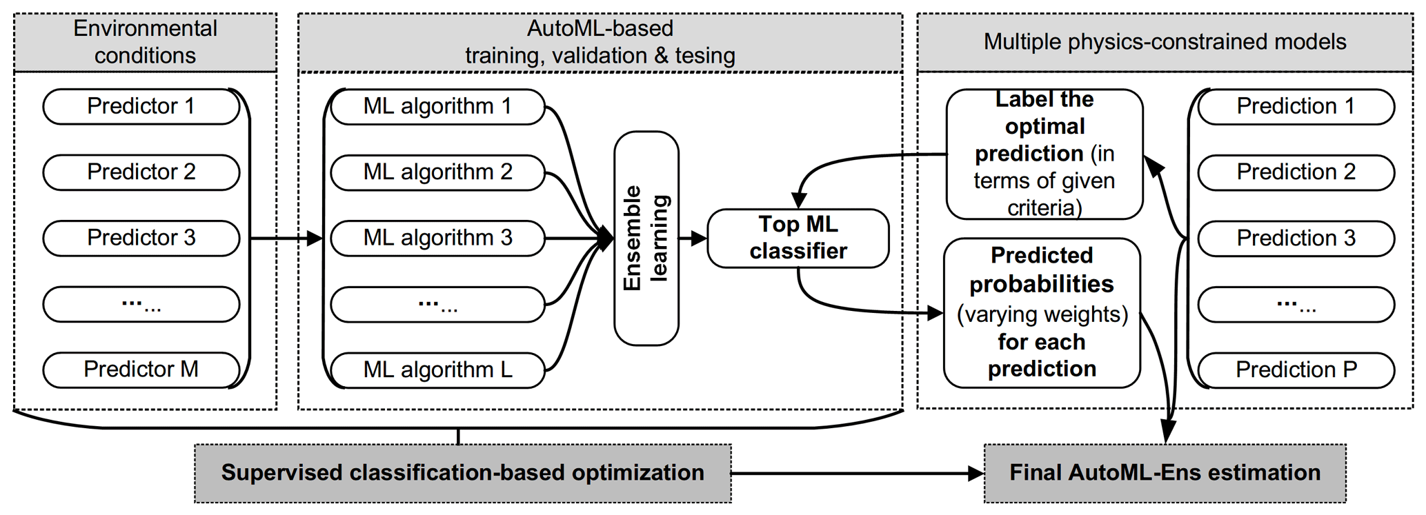
Figure 1 Procedures for building an AutoML-based ensemble framework (AutoML-Ens) to assemble geoscientific models.

To determine the ideal weights (W_k) for various models (P_k), we use an ML classifier to calculate the probability (designated as W_k) that each model is optimal in a certain environmental state. Especially, the ML classifier is trained to find the optimal models labeled as those that produce predictions with specific criteria (e.g., the least absolute error compared against observations for each sample of spatial or temporal predictions) under a specific environmental condition. Thus, ML classifiers can approximate model weights with only factors that reflect the environment after training. Here, an AutoML-based training, validation, and testing workflow is conducted to help automatically find the top classifier C_T (either a specific ML algorithm or an ensemble of a few ML algorithms $[{\mathit{M}}_l,l=\mathrm{1},\mathrm{\dots },L]$ based on the ensemble learning technique). The final AutoML-Ens estimation (Y) can subsequently be obtained by combining these candidate predictions (P) and their corresponding probabilities (i.e., varying weights W) derived by the AutoML-based C_T.

$$\begin{array}{}\text{(2)}& {\displaystyle }\mathit{Y}=[y_{\mathrm{1}},y_{\mathrm{2}},\mathrm{\dots },y_K],\text{(3)}& {\displaystyle }{y}_k={\mathit{P}}_k\times {\mathit{W}}_k,\text{(4)}& {\displaystyle }{\mathit{P}}_k=[p_{k,\mathrm{1}},p_{k,\mathrm{2}},\mathrm{\dots },p_{k,N}],\text{(5)}& {\displaystyle }{\mathit{W}}_k=[w_{k,\mathrm{1}},w_{k,\mathrm{2}},\mathrm{\dots },w_{k,N}{]}^T,\end{array}$$

where the vector Y represents the final AutoML-Ens estimation; the subscript k refers to the sample index of a model prediction that can be spatially and/or temporally varying, thus y_k denotes the ensemble of multimodel predictions for the sample k; W_k is the varying weights associated with the multiple predictions P_k for sample k. These weights are derived from an AutoML-based classifier, that is, the probability of an individual model being optimal under certain environmental conditions, and ${\sum }_{n=\mathrm{1}}^N{w}_{k,n}=\mathrm{1}$; the subscript K and N are the numbers of samples and models, respectively.

Accordingly, two distinguishing features of AutoML-Ens can be stated as follows: (1) it focuses on assembling multiple physics-constrained models to seek the optimal combination of physical and data-driven solutions, and (2) it is a supervised classification-based optimization that realizes the mapping between ML classifier-derived probabilities and dynamic adaptivity (or weights) used for an ensemble estimation to capture the nonlinear nature of targeted processes that takes full advantage of AutoML-assisted workflow. In addition, it is noteworthy that most AutoML platforms support both a collection of existing ML algorithms to select the best one and their ensembles (referred to as the pure AutoML-based ensemble, P-AutoML-Ens) based on “ensemble learning” (see Fig. 1) techniques such as bagging, boosting, dagging, and stacking (Zounemat-Kermani et al., 2021). Although both can be implemented on the AutoML platform, there are significant differences in the target ensemble objects and the strategies used between the proposed AutoML-Ens and these P-AutoML-Ens. Specifically, the core of the proposed AutoML-Ens is an ML classifier, and in order to obtain the optimal classifier, the inherent multi-classifier ensemble learning approaches in the AutoML platforms could be used. Meanwhile, for P-AutoML-Ens, the “ensemble” here is not aimed at assembling multiple models constrained by physics but the ML algorithms involved for given tasks. For example, we can select various ML algorithms to predict a target variable as a regression task without physical constraints. The AutoML tools can then help to assemble these pure data-driven algorithms inherently to make the final better estimation. Further comparison and discussion of AutoML-Ens and P-AutoML-Ens can be found in Sect. 3.2.2.

2.2 A prototype AutoML-Ens for geoscientific examples

In this study, we built a prototype AutoML-Ens in the R environment (V3.6.3) using the H₂O-AutoML platform (V3.32.1.7) in H₂O.ai (Ledell and Poiri, 2020). Note that our AutoML-Ens is not limited to the platform of H₂O-AutoML. We have chosen to use this platform because it is considered one of the leading open-source AutoML platforms according to recent benchmarking tests (Truong et al., 2019). The algorithms available in H₂O-AutoML include some of the most commonly used ML algorithms and their variants, e.g., deep neural network (DNN), distributed random forest (DRF), generalized linear model (GLM), gradient boosting machine (GBM), extreme gradient boosting (XGBoost), and extremely randomized trees (XRT). Furthermore, H₂O-AutoML provides a stacking process to find the best combination of algorithms to obtain better predictive performance, which can be recognized as one kind of realization form of P-AutoML-Ens. Detailed explanations of H₂O.ai and its H₂O-AutoML platform can be found in Ledell and Poiri (2020). Here, the common features of AutoML-Ens for the examples are summarized below. (1) In the H₂O-AutoML pipeline, the data (i.e., predictors and labels) are randomly shuffled into training (75 % with five equal-sized subsets for cross-validation) and testing (25 %). Note that due to the use of the automatic hyperparameter optimization based on Cartesian or random grid search methods in an H₂O-AutoML run (Ledell and Poiri, 2020), the maximum number of ML models was set to be 30, in addition to the two ensemble models stacked (one with the highest-performance model of each algorithm family and the other with all training models). Then, all 32 models were ranked to select the best ML classifier for final estimations. (2) Two widely used ensemble methods (that is, MEAN and BMA) were chosen for comparison; here, BMA was performed using the package “EBMAforecast” (Montgomery et al., 2017) in the R environment. In addition, the hierarchical multimodel ensemble (HME) approach proposed by Zhang et al. (2020) to estimate soil water retention parameters and the multilayer perception neural network classifier (MLP) introduced by Bai et al. (2021) with the most efficient in terms of accuracies and costs for assembling multiple physically driven cropland ET models were also investigated as baseline models, respectively. An overview of the MEAN, BMA, HME, and MLP methods we used is presented in Supplement Sect. S1) For an ML classifier, an even distribution of samples across both major and minor classes (i.e., balanced dataset) is needed to guarantee reasonable predictions of not only the majority but also classes with small sample size or extreme values (Kavzoglu, 2009). While the imbalance issue does not have a significant impact on the two examples we presented (Tables S2 and S6), we acknowledge its importance in other applications. Fortunately, the H₂O-AutoML platform provides a parameter, namely “balanced_class”, which allows for addressing class imbalance during model training. Additionally, other methods such as the synthetic minority oversampling technique (SMOTE) (Chawla et al., 2002) can also be implemented in the data preprocessing stage to generate synthetic samples for the minority class, further mitigating the class imbalance problem. (4) Regarding the performance evaluations for different models and/or ensembles, several statistical metrics, namely the Kling–Gupta efficiency (KGE) (Gupta et al., 2009; Kling et al., 2012), the coefficient of determination (R²), and the root-mean-square error (RMSE), were utilized.

3 Illustrative examples

Two real-world examples are presented in this section to test the viability of using AutoML-Ens for tackling geoscientific model ensemble problems.

3.1 Mapping global soil water retention parameters

3.1.1 Related work and data acquisition

Accurate mapping of soil water retention characteristics is essential to quantify mass-energy exchanges between the terrestrial surface and the atmosphere but is challenged by limited measurements across the globe (Dai et al., 2019b). Empirical models (i.e., PTF) often use available soil attributes. (e.g., soil texture; bulk density, BD; and soil organic matter content, OC), have been developed to estimate soil hydraulic properties, e.g., hydraulic conductivity and water retention parameters (Van Looy et al., 2017). However, despite various advancements, the reliability of PTFs for global estimates is generally uncertain, given their nonlinearities and heterogeneities (Jena et al., 2021). Thus, the assembly of multiple PTFs has been highly recommended to develop global datasets on soil hydraulic properties (Dai et al., 2019a). For instance, using a well-established global database (i.e., NCSS database), Zhang et al. (2020) proposed an ensemble of up to 13 PTFs that allows estimates of soil water retention parameters with global coverage. However, the performance of these existing generic ensembles could be further improved, as those studies assigned fixed weights to candidate PTFs regardless of regional soil conditions.

Following Zhang et al. (2020), we further tested the use of AutoML-Ens to map global soil water retention parameters. The locations of soil samples in the NCSS database cover mainly the CONUS with some data from other regions of the world (Fig. 2a), with their density distribution plotted in the USDA soil textural triangle (Fig. 2b). After data quality controls (e.g., removing some extreme soil samples with a moisture content greater than 0.6) as done by Zhang et al. (2018), 49 855 soil samples and a total of 118 599 water retention records were used with moisture content measured at matric potentials of −0.06, −0.1, −0.33, −1, −2, or −15 bar. Since Zhang et al. (2020) have provided a comprehensive summary of the selected PTFs (listed in Table S1), we focus mainly on comparing the estimates from AutoML-Ens with those from individual PTFs and their three baseline ensembles (i.e., MEAN, BMA, and HME) in this work. For the predictors of AutoML-Ens, it is noted that we do not group these PTFs according to their predictor variable requirements as in Zhang et al. (2020) but use all potential predictors (i.e., volumetric fractions [%] of sand, silt, and clay, BD [g cm⁻³], OC [%], and matric potential [bar]). Additionally, the least absolute error between the predicted and observed moisture content was selected to label the optimal PTF for each sample in the workflow. Consequently, this leads to an enclosed AutoML-assisted workflow that enables the assignment of dynamic weights for each PTF under various environmental conditions for the final ensemble estimation. Specifically, our goal was to achieve the following two objectives in this example: (1) to demonstrate the predictive capacity of AutoML-Ens, especially its unique scheme of assigning dynamic weights to candidate members, and (2) to produce a set of improved global maps of key parameters of soil water retention characteristics (i.e., field capacity and wilting points) for global applications.

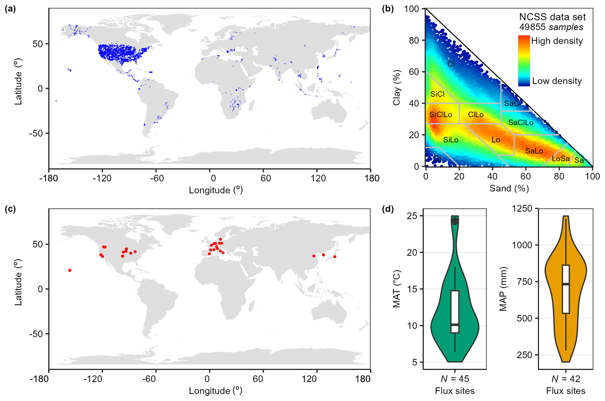
Figure 2 (a) Locations of selected soil samples from the National Cooperative Soil Survey Characterization (NCSS) covering the conterminous United States (87.7 % of the data) and other regions of the globe (12.3 % of the data) and their density distribution plotted in (b) the US Department of Agriculture soil textural triangle (USDA). (c) Locations of 47 eddy covariance flux sites that cover croplands from AmeriFlux, AsiaFlux, FLUXNET, and the European Flux Database Cluster and (d) their mean annual temperature (MAT, ^∘C) and mean annual precipitation (MAP, mm) distributions.

3.1.2 Necessity of assigning dynamic weights in ensembles

Figure 3 shows how R² and RMSE of the soil water content from the 13 PTFs and their ensembles (i.e., MEAN, BMA, HME, and AutoML-Ens) vary across the datasets (training, testing, or overall data) and wide environmental gradients. Note that AutoML-Ens here was defined as the leader-one ranking among all the 32 ML models involved in the AutoML workflow, which was selected to be the stacked ensemble based on all models derived from the H₂O-AutoML platform. Results demonstrate that each PTF has distinct strengths and weaknesses in modeling underneath the data, such as the PTF with relatively better performance or the worse one, i.e., Wösten PTF (Wösten et al., 1999) and Carsel & Parrish PTF (Carsel and Parrish, 1988), respectively, for both the training and testing data. Further inspection indicated that the four ensembles achieved improved predictive capabilities than any single PTF used in the analyzes, where BMA and HME yielded better performances than MEAN. Meanwhile, AutoML-Ens was superior on the overall data with the largest positive R² difference value of 0.075 (improved by 9 % from 0.797 to 0.872) and the lowest negative RMSE difference value of −0.012 m³ m⁻³ (reduced by 22 % from 0.055 to 0.043 m³ m⁻³) compared to the MEAN ensemble (considered the benchmark). We further explored the variations in the R² and RMSE values of the overall 17 models under different environmental conditions (that is, different classes of USDA soil texture, matric potential, BD, and OC, as shown in Fig. 3c–j, respectively). Figure S1 presents a detailed prediction comparison of 13 individual PTFs and 6 individual ML algorithms along the environmental gradients. The general conclusions remain the same, indicating that different PTFs and their ensembles present various abilities, as expected in terms of the changing environmental gradients. More precisely, both the predictive capacities of individual PTFs and their ensembles appear to have a high sensitivity to the selected predictors. For instance, the performance of these predictions improves with increasing BD and OC values. It also suggests that those environmental factors with significant influences on model performance should not be ignored when developing models and simulating or predicting variables.

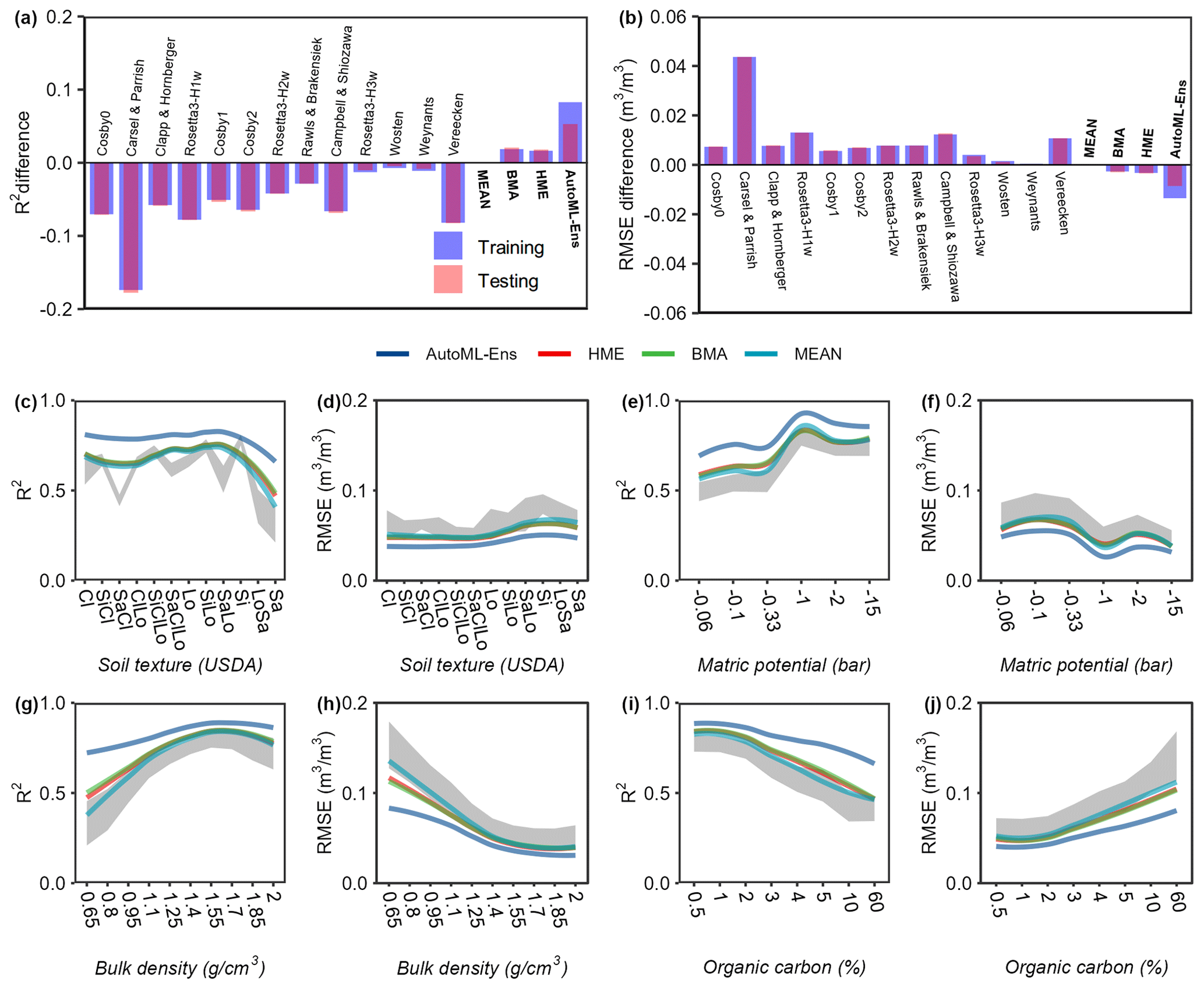
Figure 3 Difference in performance metrics (R² (a) and RMSE (b)) between MEAN and all 17 models, including individual PTFs and model ensembles (in bold font) for training and testing data. A positive R² or negative RMSE difference means that the model yields a larger R² or smaller RMSE, indicating the better performance of the model than MEAN (considered the benchmark). R² (c, e, g, i) and RMSE (d, f, h, j) when the moisture content estimates of different ensemble approaches were compared with observations (including all training and testing data) under various environmental conditions (six variables, among which the content of sand, silt, and clay was expressed together in terms of USDA soil texture classes) that were represented by predictors for AutoML-Ens. The gray band denotes the uncertainties calculated as the mean ± standard deviation of the R² (or RMSE) values of the 13 selected PTFs.

In addition, ensemble PTFs are more practical due to their higher reliability and error compensation among ensemble members. For instance, BMA weights each PTF according to its posterior model probability and offers a fixed weight for each PTF, potentially reducing the uncertainties in individual models. However, the fixed weight assigned by these conventional ensembles (MEAN, BMA, and HME; see Supplement Sect. S1) may not fully leverage the strengths of a PTF since it is based on the assumption that the performance of a PTF is constant under all environmental conditions. The fact is that multiple soil factors nonlinearly regulate the processes in soil water retention and further result in various performances of individual PTFs. On the contrary, the results show clear advantages of AutoML-Ens over these conventional ensembles on different datasets (both the training data and the testing data) and across various environmental constraints than other ensembles and individual PTFs, highlighting its relatively better suitability for assembling multiple PTFs for estimating soil water retention parameters.

Furthermore, a set of global soil water retention parameters (with a resolution of 10 km) was produced at different soil depths (that is, 0–5, 5–15, 15–30, 30–60, 60–100, and 100–200 cm) using the SoilGrids soil composition database (Hengl et al., 2014, 2017) as input for the newly proposed AutoML-Ens. Meanwhile, the ensemble estimates based on HME were also generated for comparison (partly shown in Fig. 4). Here we chose two key variables, i.e., moisture content at −0.33 and −15 bar, which are commonly used to indicate field capacity and permanent wilting point (Jury and Horton, 2004), respectively, for comparison. It can be seen in Fig. 4 that despite the considerable discrepancies in the values identified in northern high-latitude regions (>50^∘ N), there was a similar spatial pattern between the ensemble estimations of HME and AutoML-Ens in most parts of the globe. Although both approaches were developed on the basis of the same independently measured water retention data, the ensemble schemes for optimized estimations are different. A major difference is that HME was developed for the entire dataset, although a bootstrap resampling process was adopted in optimization, in which a set of fixed weights was assigned to each PTF in all soil conditions, so that the optimized results depended highly on the measurements. However, AutoML-Ens depicts soil conditions (predictors) as a continuum, with the aim of finding the optimal PTF under certain environmental conditions by assigning dynamic weights for the candidate PTFs. In other words, AutoML-Ens has learned the optimal adaptation between the predictors (environmental constraints) and the predictions (PTFs), which allows for stronger extrapolation and increased generalization for approaching other issues or regions. Thus, due to the limited distribution of NCSS soil samples in northern high-latitude regions, a significant difference in the estimations from the two ensemble methods with different generalization abilities can be expected.

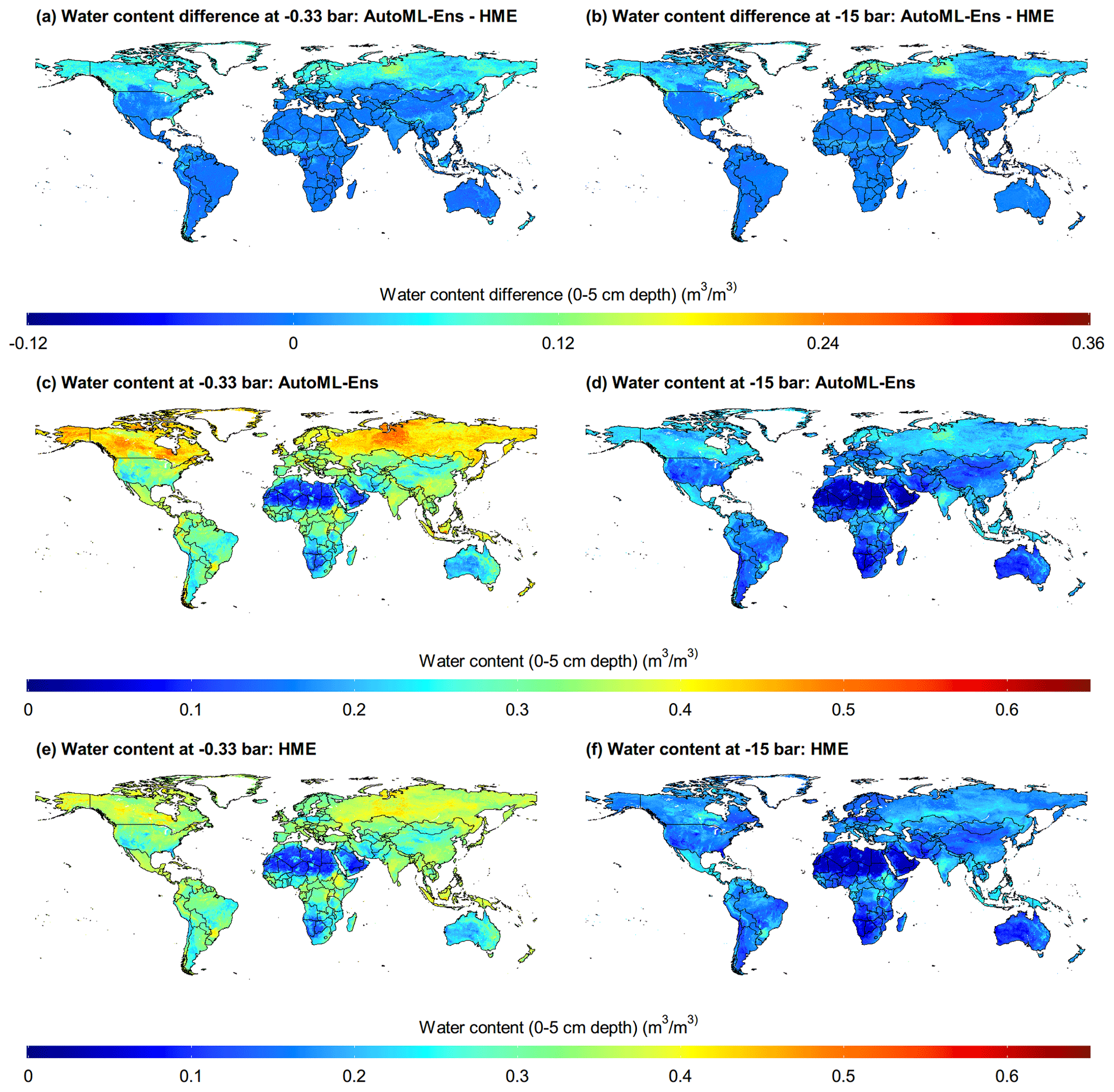
Figure 4 Global maps (with 10 km resolution) of moisture content (0–5 cm depth) with a matric potential of −0.33 bar (a, c, e) and −15 bar (b, d, f) delivered based on the soil composition database of SoilGrids. The first-row panels show the differences in moisture content between the prediction of AutoML-Ens and HME. The second- and third-row panels are ensemble predictions from AutoML-Ens and HME, respectively.

Another form of evidence on the necessity of enabling dynamic weights for an ensemble is provided in Fig. 5a, which directly reflects the varying weights assigned for each PTF based on the overall data samples. As can be seen, the weights of each PTF fluctuated dramatically with the range from approximately 0 to 1. In addition, Fig. 5b and c illustrate global maps of PTF with the largest weight derived from AutoML-Ens among the 13 selected PTFs at a matric potential of −0.33 and −15 bar, respectively. For different soil retention parameters (e.g., water content at different matric potentials), even at the same spatial location, their PTFs with the largest weight are significantly different. These again suggested that no PTF had been found to be consistently better than the other under different environmental conditions. Therefore, if fixed weights are used in assembling these multiple PTFs for different parameters estimation, e.g., as the HME approach does, it will inevitably lead to the failure to use the advantages of different PTFs fully. However, this evaluation has some limitations because the same database (i.e., the NCSS database) was utilized to compile HME and AutoML-Ens, indicating that the two methods were not independently validated. Other evaluations and applications, for example, as input parameters to drive regional and global LSMs, need to be further conducted to indicate which product is more accurate and reliable. Furthermore, it should be noted that regional- to global-scale soil parameters with a higher spatial resolution of 90 m to 1 km can also be generated through the workflow based on various data sources (e.g., recently released national gridded soil property maps of China; Liu et al., 2021) in addition to the SoilGrids. We expect that the AutoML-Ens-derived soil parameter datasets can be helpful for a variety of purposes, such as improving the performances of Earth system models.

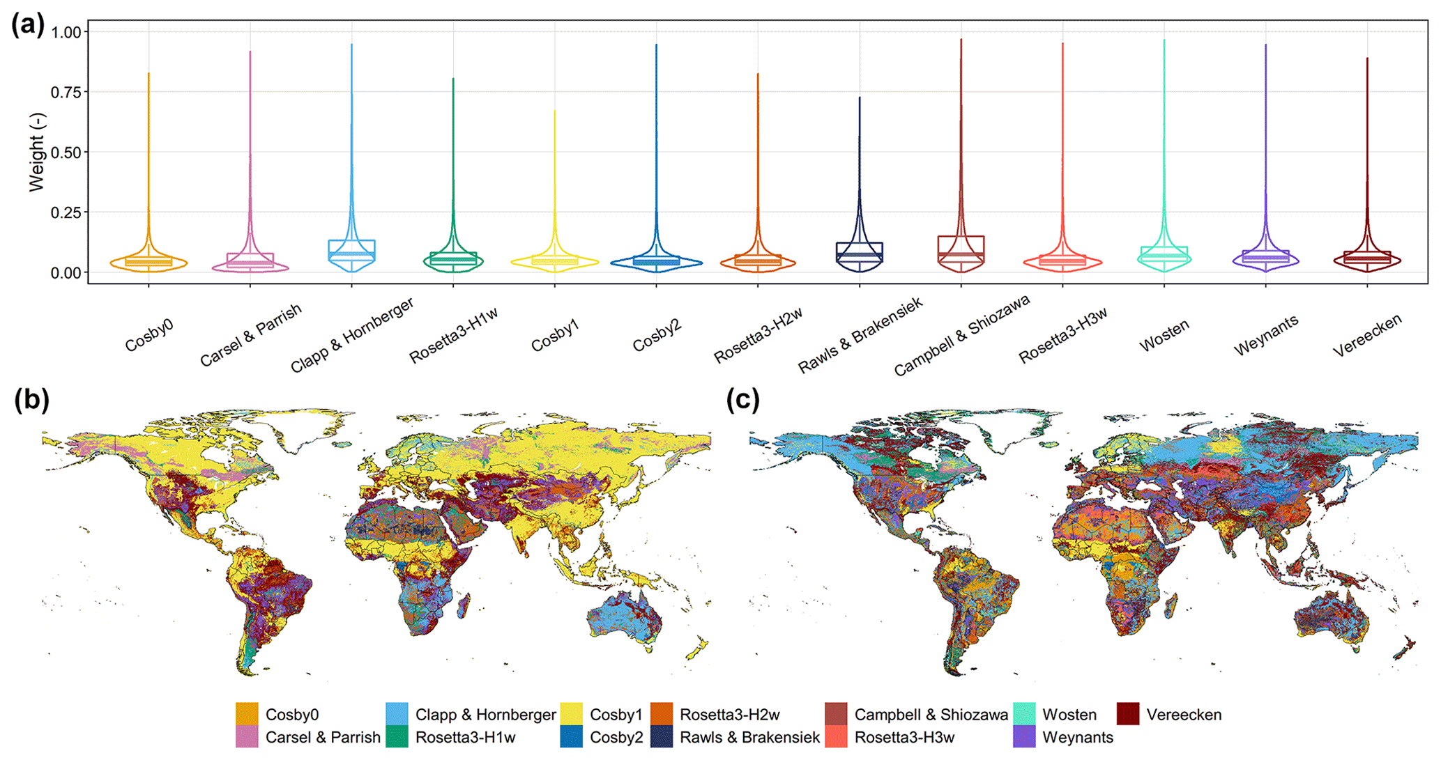
Figure 5 Varying weights assigned for each PTF under the overall data samples (a). Global maps (at 10 km resolution) of PTF with the largest weight among the 13 selected PTFs at a matric potential of −0.33 bar (b) and −15 bar (c) delivered based on the soil composition database of SoilGrids through AutoML-Ens.

In general, how to fully use the strength of individual models under certain environmental conditions is vital for making better ensemble estimates. This example emphasizes the necessity of assigning optimal dynamic weights in ensemble approaches, which also demonstrates the great potential of AutoML-Ens to map global soil water retention-like parameters in geosciences. More specifically, for example, some observations may have already been used in calibrating the physics-based models with varying degrees, resulting in diverse performances of these models under certain environmental conditions. While the final goal of the numerous ensemble approaches is the same, that is, to obtain the final improved estimations, they are different in ensemble strategies. It can be expected that when a physics-based model has involved more observations (i.e., more approximate to observations), the model's weight in an ensemble is relatively large. This is especially true for conventional ensemble methods that provide fixed weights for candidate models under all conditions. However, with a varying-weight strategy under certain conditions, the advanced AutoML-Ens would not worship the model that integrates more observations nor exclude the one that may perform well under certain conditions but does not have observation constraints. Hence, the AutoML-Ens' generalization ability is worth emphasizing.

3.1.3 Does the classification accuracy matter?

Moreover, it is worth noting that the essence of AutoML-Ens is a kind of AutoML-assisted classifier, which also generates classification accuracy. However, improving this accuracy is not the overarching objective of AutoML-Ens. Poor accuracy may result from the uneven distribution of available data samples, their low representative ability, and inter-model similarities and dependencies (Holtanová et al., 2019). The similarities within a multi-model ensemble in particular may result from using the same set of data samples, sharing certain components, or being based on the same hypothesis. This makes it difficult to justify the independence assumption between ensemble members, further leading to poor classification. Regarding the similarities between these 13 PTFs, it should be noted that not all PTFs were developed using independent calibration datasets, and the development legacy is not always evident. For example, data used to establish the Rawls & Brakensiek (Rawls and Brakensiek, 1985) PTF was used by Carsel & Parrish and partially for the Rosetta3 (Zhang and Schaap, 2017) PTFs. The Vereecken (Vereecken et al., 1989) data was used for the Weynants (Weynants et al., 2009) PTF and also included in the database used to develop Rosetta3 PTFs. Moreover, various ways exist by which PTFs can be grouped or distinguished, such as the predictor variable requirements (e.g., requiring the variable BD and/or OC or not) and techniques utilized (e.g., lookup table, regression, and neural networks) (Zhang et al., 2020). Furthermore, taking the derived soil water content at −0.33 bar (0–5 cm depth) as an example, the largest weights (Fig. 6a) and the difference between the largest and the second-largest weights (Fig. 6b) for specific PTFs are relatively small in most regions of the world. The largest weight values below 0.3 and the weight difference below 0.1 accounted for approximately 71.0 % and 56.6 % of the total global land area, respectively. The direct cause of this result is the similarities between these PTFs mentioned above. However, regardless of how the selected classifier performs, the sum of the varying weights (i.e., derived probabilities) is equal to 1 under all specified conditions. For instance, if taking the mean per class error, which indicates misclassification of the data across the classes, as an indicator, it ranges from 77 % to 90 % for the 32 trained classifiers in this example. More precisely, it does not perform very well, even for the leader model in the AutoML-Ens workflow, but has been proven to be a promising ensemble relative to others. Therefore, efforts could be made to reduce the similarities within candidate models to obtain a higher classification accuracy. Moreover, once a good classification accuracy is obtained among the training and testing datasets, the linkage between the predictors and the label in the workflow will be more clearly determined, which can help implement and/or modify these candidate models appropriately.

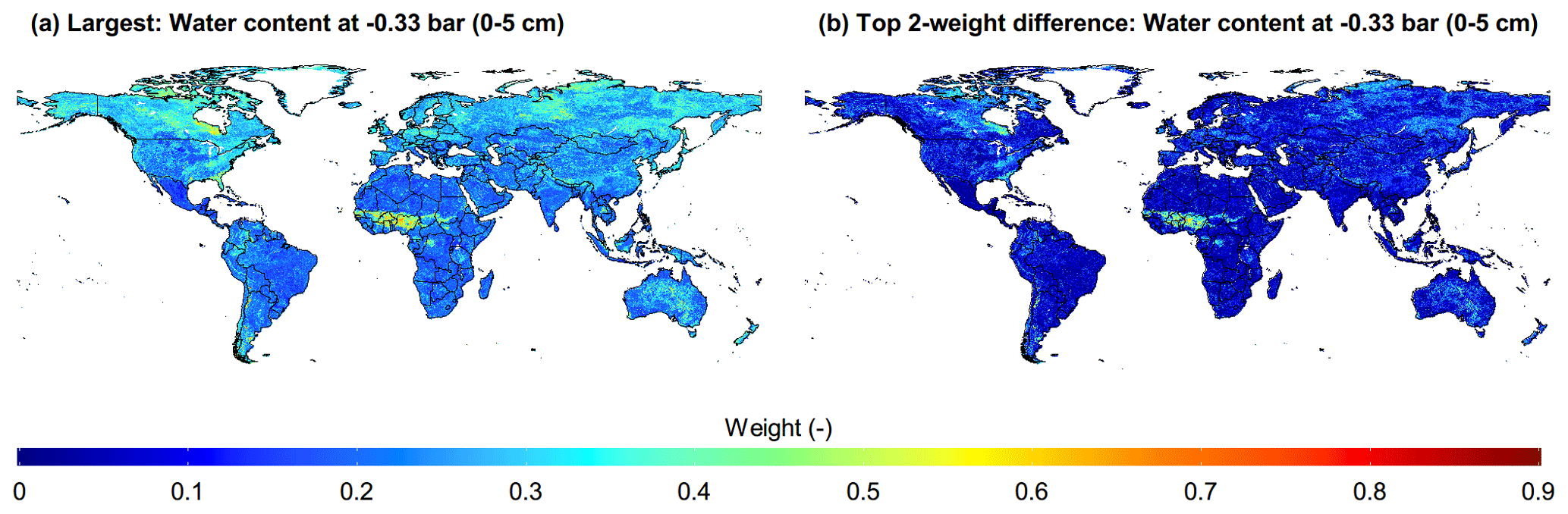
Figure 6 Global maps (at 10 km resolution) of the largest weight (a) and the top two weight difference values for specific PTF (b) at a matric potential of −0.33 bar (0–5 cm depth) delivered based on the soil composition database of SoilGrids through AutoML-Ens.

3.2 Improving remotely sensed cropland ET estimates

3.2.1 Related work and data acquisition

Accurate delineation of spatiotemporal variations in land ET is essential to appraise many geoscience issues, such as the ecosystem responses to global environmental changes, but often challenging because of its highly dynamic and nonlinear response in nature (Fisher et al., 2017; Pascolini-Campbell et al., 2021; Wang and Dickinson, 2012). Given that recent studies have shown that a multimodel ensemble can outperform individual ET models (e.g., Bai et al., 2021), the objective of this example was to improve cropland ET estimates globally by using the AutoML-Ens framework. Following Bai et al. (2021), observations from 47 cropland eddy covariance flux sites (listed in Table S4) covering various environmental gradients and three continents were used (see Fig. 2c–d). Estimates from six physical ET models based on remote sensing, namely PT-JPL, PT-DTsR, SEBS, STIC, RS-WBPM, and EVI-PM, were adopted as candidate predictions. An overview of these six ET models is presented in Table S5. A total of 11 variables (i.e., the predictors of AutoML-Ens) jointly constraining ET based on different biophysical principles were considered, including several widely used meteorological and remote sensing factors: daily precipitation rate (mm d⁻¹), air temperature (^∘C), net radiation (W m⁻²), vapor pressure deficit (hPa), wind speed (m s⁻¹), normalized vegetation index (NDVI), enhanced vegetation index (EVI), soil adjusted vegetation index (SAVI), land surface temperature during the day (daytime land surface temperature (LST), K), diurnal range of LST (^∘C), and water stress factor (0–1) from the RS-WBPM model (Bai et al., 2018) representing meteorological drought. After data checking and filtering, a total of 83 621 records were used for ensembles and evaluations. Moreover, the lowest absolute errors between the daily scale latent heat flux (LE) observations and the corresponding estimates from individual ET models were used to label the optimal physically based ET prediction in the AutoML-Ens workflow.

3.2.2 Advantage of an AutoML-based workflow

Similar to the previous example results, AutoML-Ens performed much better than conventional approaches (i.e., MEAN, BMA) for assembling multiple physically based ET models, as it yielded larger R² and smaller RMSE (Fig. 7a–b). Taking the MEAN ensemble as the benchmark, AutoML-Ens was superior on the overall data with the largest positive R² difference value of 0.15 (improved by 21.4 % from 0.70 to 0.85) and the lowest negative RMSE difference value of −7.98 W m⁻² (reduced by 32.8 % from 24.36 to 16.38 W m⁻²). These results again suggested the importance of assigning varying weights for an ensemble because the six physically driven ET models exhibited much more complex capabilities (taking KGE as the criterion) under different environmental gradients (see Fig. 7c–m). However, some repeated evaluation results to demonstrate AutoML-Ens were omitted here. Instead, another point worth noting in this example was why the ML-based ensembles (i.e., MLP and AutoML-Ens) using almost identical datasets and procedures presented considerable differences in terms of accuracies. As introduced by Bai et al. (2021), four different ML classifiers, namely k-nearest neighbors (KNN), MLP, random forest (RF), and support vector machine (SVM), were utilized to assemble ET models. These classifiers have different mechanisms and various schemes, thus resulting in different efficiencies among each other. On the one hand, it indicated that if other advanced ML algorithms were adopted as classifiers, MLP might not be further recognized as the best. However, on the other hand, it is too challenging to manually select the best ML classifier, which needs the assistance of AutoML in complex pipelines. Moreover, the ranking of 32 models involved in the AutoML-Ens workflow with regard to the mean per class error and the corresponding performance metrics of their ensemble predictions are presented in Table 1. As can be seen, the best model in terms of lowest classification error was selected to be the stacked ensemble based on all models, followed by the stacked ensemble based on the best of family, XRT, DRF, GBM, XGBoost, and DNN, as well as their variants with different hyperparameters. However, the ranking of performance metrics for the final ensemble predictions differs from the classification accuracy of individual classifiers. While the top classifier, Stacked_Ensemble_All_ Models, demonstrates high predictive performance, the XGBoost_grid_1_model_8 classifier achieves the best ensemble prediction, with an R² value of 0.87 and an RMSE of 15.03 W m⁻². This result further confirms the primary objective of AutoML-Ens, which is not solely focused on achieving optimal classification results but rather on finding the optimal utilization and combination of ML algorithms to obtain better predictive performance. Consequently, this example demonstrated and emphasized another unique feature of the proposed AutoML-Ens framework, that is, taking full advantage of the AutoML-assisted workflow. As such, AutoML-Ens, which better incorporates the capacities of diverse biophysical mechanisms and environmental variables, has the potential to improve the estimations of global cropland ET.

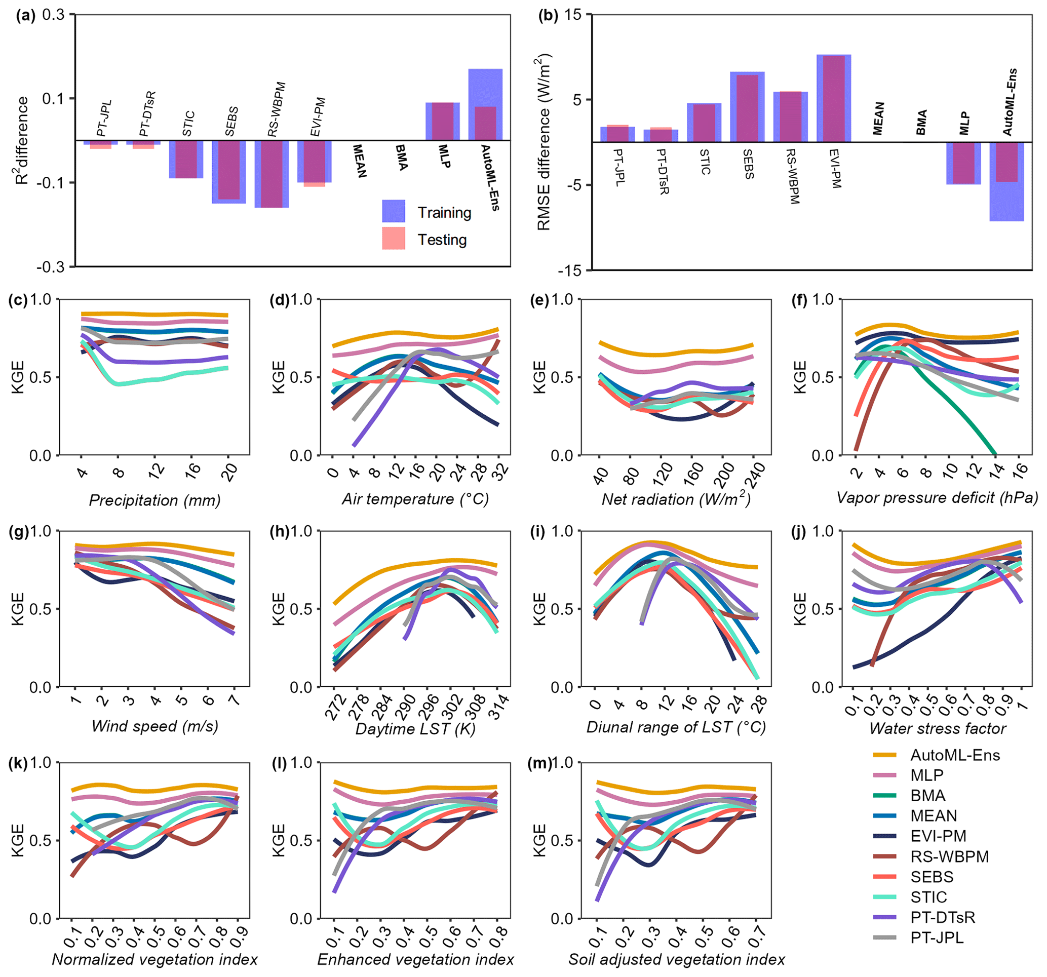
Figure 7 Difference in performance metrics (R² (a) and RMSE (b)) between MEAN and all 10 models, including six physically based ET models and four ensembles (in bold font) for training and testing data. A positive R² or negative RMSE difference means that the model yields a larger R² or smaller RMSE, indicating the better performance of the model than MEAN (considered the benchmark). KGE (c–m) when ET estimates from the 10 models were compared against observations (including all training and testing data) under various environmental conditions (11 variables) that were represented by predictors for AutoML-Ens.

Table 1 Ranking of the 32 models involved in the AutoML-Ens workflow with respect to the mean per class error and their corresponding performance metrics (R² and RMSE) of their ensemble predictions.

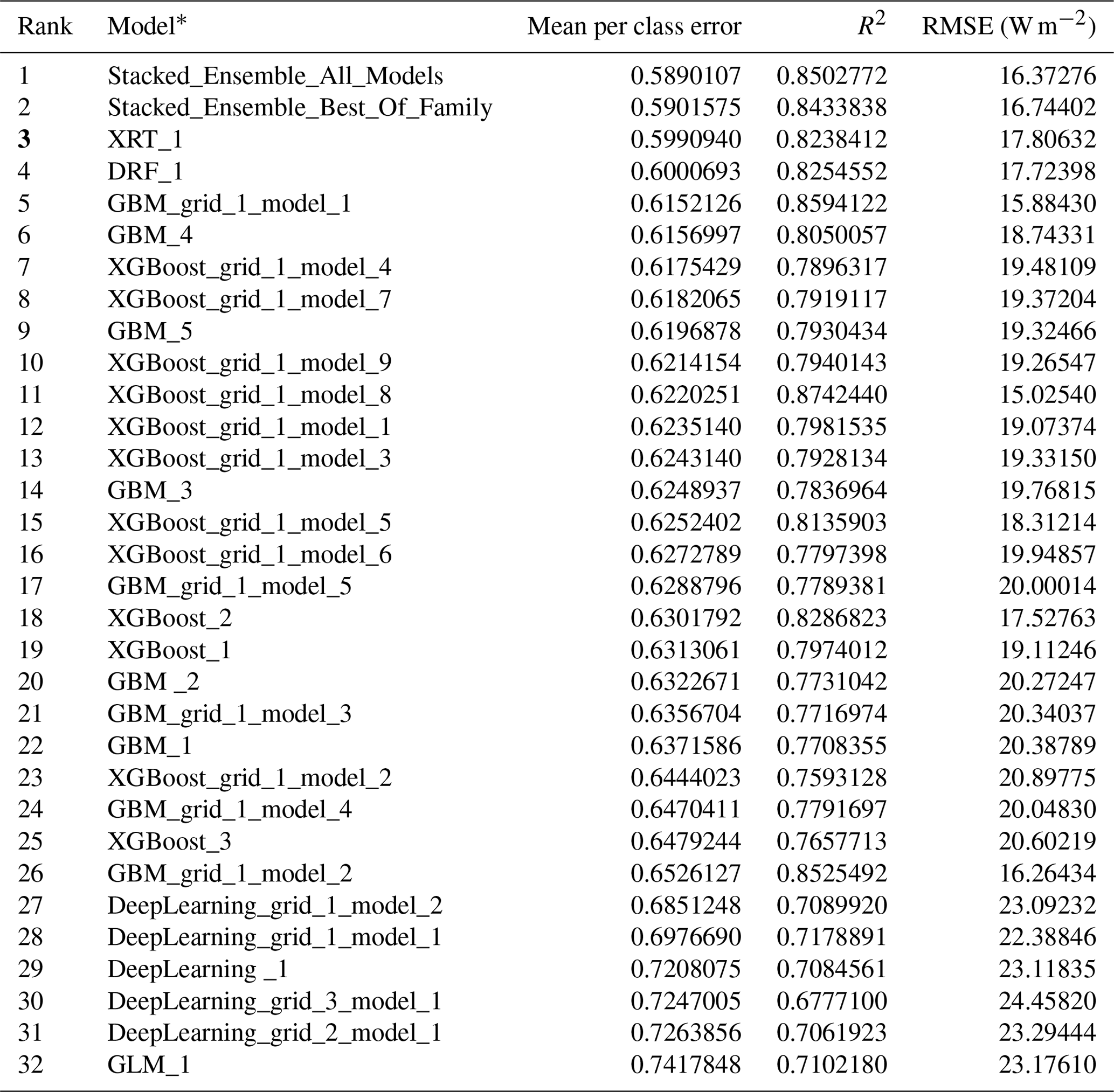
^* The same ML model with different number signs indicates their variants with different hyperparameters.

3.2.3 Perspective on combining ML and physical modeling

Furthermore, since ML regression algorithms have been widely applied in various geoscience domains and H₂O-AutoML provides P-AutoML-Ens mentioned above based on a stacking process for assembling these algorithms, it is interesting to address the following two questions. (1) How does the predictive capability of AutoML-Ens compare with those of P-AutoML-Ens? (2) What causes the differences between the performance exhibited by AutoML-Ens and P-AutoML-Ens? To this end, we additionally built two P-AutoML-Ens workflows, taking either the observed daily scale LE or $\mathrm{Rn}-H-G$ directly as labels for predicting ET as regression tasks (i.e., P-AutoML-Ens_LE and P-AutoML-Ens_Rn_H_G). Note that Rn denotes net radiation; H and G represent sensible heat flux and ground heat flux, respectively; and in terms of theory, “$\mathit{LE}=\mathrm{Rn}-H-G$”. However, due to the widely acknowledged energy balance closure problem, LE is not equal but highly relevant to $\mathrm{Rn}-H-G$ for most flux observations, with an R² (RMSE) value of 0.76 (26.5 W m⁻²) obtained in this study. The environmental conditions (i.e., predictors) for the two workflows were the same as those for AutoML-Ens. The comparison results are presented in Fig. 8. As shown in the left part of Fig. 8a–b, ET estimates from any of the conventional ensemble methods (i.e., MEAN and BMA), the ML classifier-based ensembles with dynamic weights (i.e., MLP and AutoML-Ens), or P-AutoML-Ens_LE presented better performance metrics than any single physically based ET model compared against LE observations. However, it is worth noting that the performance measures of different ET models and ensemble approaches may vary depending on the focused regions, ecosystem types, temporal scale of validation, testing strategies, and so on. Moreover, P-AutoML-Ens_LE performed better than AutoML-Ens with slightly larger R² and smaller RMSE, indicating that the simple regression-based P-AutoML-Ens could replace AutoML-Ens with complex physics constraints. However, this was proven to be an illusion when we further inspected the predictive capabilities of these two types of ensemble approaches. It was found that AutoML-Ens showed comparable performances when validated with either the observed LE or Rn-H-G series; that is, it conserved the energy balance or followed physical constraints. In contrast, significant discrepancies in performance metrics existed between the two P-AutoML-Ens workflows, even when the estimations from P-AutoML-Ens_Rn_H_G were compared with the observed Rn-H-G series. This suggested that an internal deficiency existed in these P-AutoML-Ens; that is, they cannot precisely conserve the energy budget, limiting their extrapolation and out-of-sample generalization capacities (also discussed in Zhao et al., 2019). Therefore, comparisons of AutoML-Ens with P-AutoML-Ens should not be limited to a performance perspective, leading to false conclusions. Here, we prefer to emphasize the potential of the AutoML-Ens framework, since it not only provides an effective alternative for solving various geoscientific model ensemble problems but is well controlled by fundamental physics in geosciences. Overall, it is worth adding here as recent studies suggested (e.g., Jia et al., 2021; Karpatne et al., 2017; Reichstein et al., 2019) that physically based models and ML models will not be mutually incompatible. Instead, combining ML and physical modeling might yield a more promising but equally demanding solution.

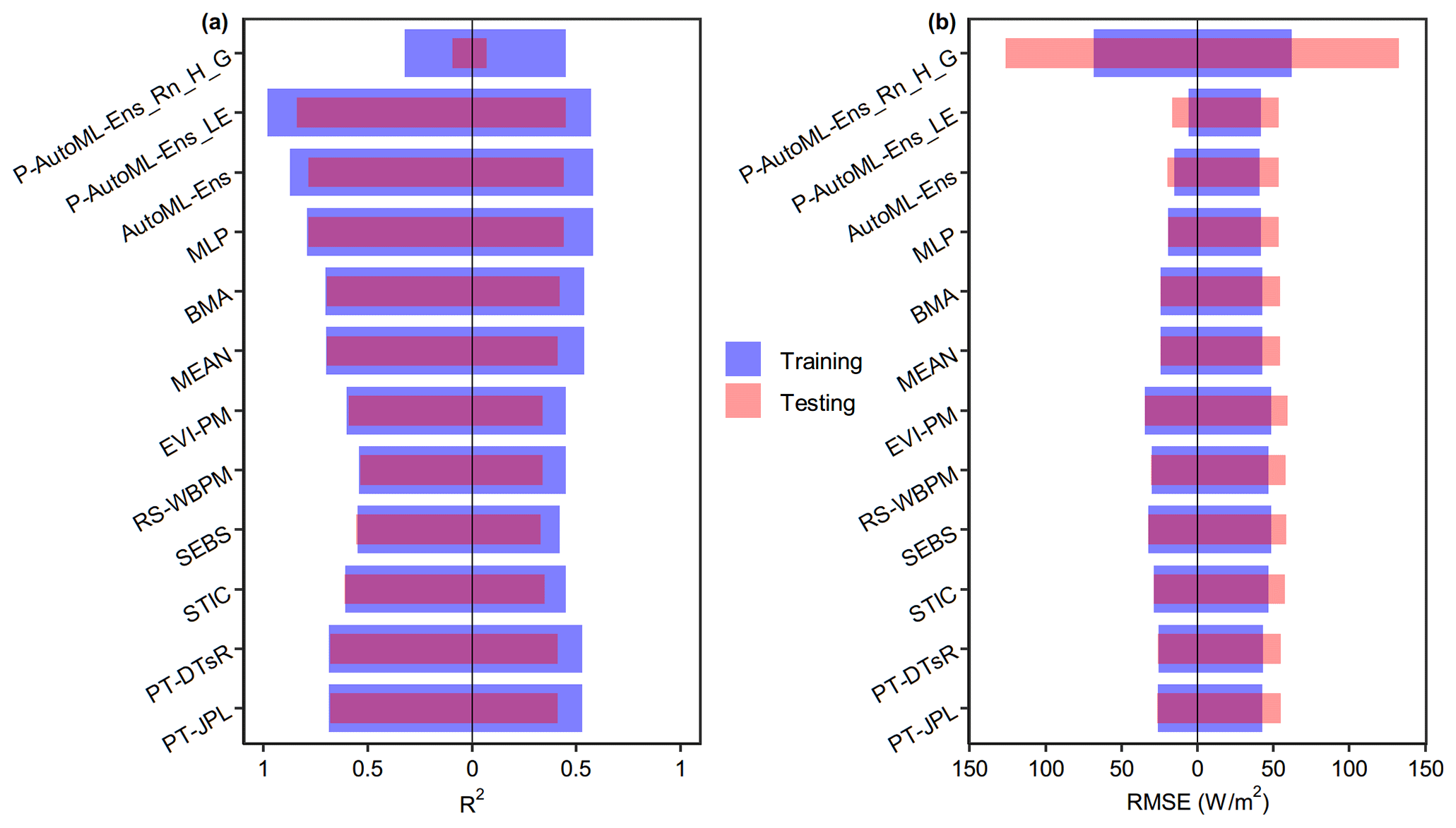
Figure 8 Performance metrics (R² (a) and RMSE (b)) when ET estimates from a total of 12 models, including six individual physically based ET models and their four ensembles (i.e., MEAN, BMA, MLP, and AutoML) and two pure AutoML-based ensembles taking either the observed daily scale LE or $\mathrm{Rn}-H-G$ as labels (i.e., P-AutoML-Ens_LE or P-AutoML-Ens_Rn_H_G) in regression tasks, were compared against observations (LE (a) and $\mathrm{Rn}-H-G$ (b)) of the training and testing data.

4 Conclusions

The past few decades have witnessed unprecedented improvements in geoscientific modeling solutions, from statistical and box models to Earth system models. However, existing models frequently utilize a few environmental factors to constrain physical processes that cannot capture fully their nonlinear nature, which changes greatly across spatiotemporal domains. This is particularly true in regions with dynamic changes under the joint impact of climate change and human activity. In this study, we introduced an AutoML-Ens framework to address this issue, which could help to maximize the strengths of individual models and the ability of the unique environmental variables utilized in these models to better characterize processes. The findings lead to the following conclusions.

1. The two illustrative applications of AutoML-Ens comprehensively demonstrated its better potential to improve estimations. Compared to conventional ensemble approaches, AutoML-Ens produced a larger R² and KGE and smaller RMSE, for example, in estimating soil water retention parameters and cropland ET.

2. Assigning dynamic weights to each candidate member under wide environmental conditions is essential for a better ensemble than the conventional ensemble approaches (e.g., MEAN and BMA), which usually provide fixed weights according to several statistical criteria. Specially, we proposed a novel and general strategy, i.e., mapping between ML classifier-derived probabilities and dynamic weights, in the framework. While other approaches, e.g., the known kriging methods, can also provide such probabilities, and they can be regarded as possible extensions of the framework.

3. Similarities within a multi-model ensemble are responsible for poor ML classification accuracy. Efforts could be devoted to reducing these similarities to obtain a higher classification accuracy. A good classification also indicates a more evident linkage between the predictors and the label in AutoML-Ens, which can, in turn, help improve these ensemble members accordingly. However, this is another critical issue that needs further exploration and is not the overarching objective of AutoML-Ens.

4. Although the assignment of dynamic weights could help improve the ensembles, they are primarily based on the efficiency of ML classifiers, which require substantial human interventions for, e.g., hyperparameter tuning, if done manually. Thus, taking full advantage of AutoML-assisted workflow, also one of the distinctive features of AutoML-Ens, provides a good example to guide future research in the area.

5. Pure AutoML-based (or data-driven) ensembles may appear largely inconsistent with known physics (e.g., conservation of energy or mass), leading to an illusion of superiority in model performance. Specifically, we call for the combination of data-driven approaches with physics constraints when resolving various geoscientific model ensemble issues.