Modeling sensitivities of thermally and hydraulically driven ice stream surge cycling

Modeling ice sheet instabilities is a numerical challenge of potentially high real-world relevance. Yet, differentiating between the impacts of model physics, numerical implementation choices, and numerical errors is not straightforward. Here, we use an idealized North American geometry and climate representation (similarly to the HEINO (Heinrich Event INtercOmparison) experiments – Calov et al., 2010) to examine the process and numerical sensitivity of ice stream surge cycling in ice flow models. Through sensitivity tests, we identify some numerical requirements for a more robust model configuration for such contexts. To partly address model-specific dependencies, we use both the Glacial Systems Model (GSM) and the Parallel Ice Sheet Model (PISM). We show that modeled surge characteristics are resolution dependent, though they converge (decreased differences between resolutions) at finer horizontal grid resolutions. Discrepancies between fine and coarse horizontal grid resolutions can be reduced by incorporating sliding at sub-freezing temperatures. The inclusion of basal hydrology increases the ice volume lost during surges, whereas the dampening of basal-temperature changes due to a bed thermal model leads to a decrease.

1 Introduction

1.1 Motivation and background

The use of ice sheet models has grown by at least 1 order of magnitude over the last 2 decades. The relevance of such modeling studies to the actual physical system can be unclear without careful consideration and testing of numerical aspects and implementations. This is especially true when modeling the highly non-linear ice sheet surge instability, which has significant implications not only for the ice sheet itself but also for the climate. In fact, it is often difficult to assess whether model results are physically significant (effects of physical system processes), a consequence of model-specific numerical choices, or a combination of both. Whether ice sheet instabilities observed in numerical simulations are the result of physical instabilities of the underlying continuum models or of spurious effects of the discretization and numerical implementation of said models has long been debated (e.g., Payne et al., 2000; Hindmarsh, 2009) and is a consequential matter. The present study is concerned with characterizing the impact of model physics, numerical choices, and numerical errors on ice stream surge cycling.

Binge–purge ice stream cycling was first introduced in the glaciological literature by MacAyeal (1993) as an explanation for Heinrich events arising from the former Laurentide Ice Sheet (LIS) in the Hudson Bay–Hudson Strait region. The key idea is that the ice stream gradually grows to a threshold thickness (binge phase) driven by surface accumulation. Once the ice stream is thick enough to sufficiently isolate the ice stream base from the cold surface, heat from geothermal and deformation work sources can slowly bring the basal temperature to the pressure-melting point. The bottom layer of the ice stream is no longer frozen to the bed and thus enables basal sliding. Localized warm-based ice streaming increases the ice stream surface gradient (steeper slope) at the warm–cold-based transition point, leading to an increase in driving stress. The resultant increase of heat from deformation work can warm the surrounding ice (close) to the pressure-melting point, thus enabling (sub-temperate) basal sliding (Fowler, 1986). When the melting point is reached, the presence of water at the ice sheet–bed interface (Fowler and Schiavi, 1998) and in a deformable sediment layer (Bueler and Brown, 2009) can further increase sliding velocities. Instead of the slow deformation flow (ice creep), the ice stream now flows rapidly (purge phase). As a consequence of the high ice velocities, the ice stream thins, and cold ice is advected from either upstream or the lateral boundaries of the ice stream. Cold ice advection in combination with changing heat source contributions (from both deformation work and basal sliding) and lowering of the pressure-melting point as ice thins eventually leads to refreezing of the ice–bed interface. The first localized frozen patch of ice acts as a sticky spot, supporting some of the driving stress and decreasing the velocities and heat production in the adjacent ice. This marks the end of the surge, thus enabling the ice stream to enter the next binge phase. Whether hydraulically or thermally driven, these activation (purge) and stagnation (binge) phases can alternate in a quasi-periodic fashion (e.g., Souček and Martinec, 2011) – this is what we refer to as ice stream surge cycling in the remainder of this paper.

As a result of the physics involved and the behaviors expected, modeling of ice stream surge cycling is challenging. The challenges entail, among others, rapid surge onset, high ice velocities, and non-linear (thermo-viscous, hydraulic, and thermo-frictional) feedbacks. In addition to the physical complexity, further challenges arise in the numerical modeling of ice stream surge cycling, whether in terms of model choices (e.g., choice of mechanical model, thermal modeling of the substrate, accounting for sub-glacial hydrology) and/or in terms of their numerical implementation (e.g., grid size, convergence under grid refinement).

Our focus here is on the challenges arising from numerical modeling, both those related to the physical system being modeled and those related to the numerical implementation. The effects of different approximations of the Stokes equations have been previously addressed (e.g., Brinkerhoff and Johnson, 2015) and are therefore not discussed here.

The discretization and related numerical implementation choices (e.g., grid resolution and grid orientation) have been shown to affect numerical results (e.g., Calov et al., 2010; Roberts et al., 2016; Ziemen et al., 2019). As far as the choice of grid is concerned, Ziemen et al. (2019), for example, find a constantly active ice stream at 40 km grid resolution and oscillatory behavior at 20 km grid resolution. They argue that this finer grid resolution is necessary to resolve the Hudson Strait properly. A few other studies examine the effect of different grid resolutions on surge behavior (e.g., Payne and Dongelmans, 1997; Greve et al., 2006; Van Pelt and Oerlemans, 2012; Brinkerhoff and Johnson, 2015; Roberts et al., 2016), but an in-depth numerical analysis of Hudson Strait ice stream surge cycling (to whatever idealized form) is entirely absent from the literature. In terms of grid rotation, Greve et al. (2006) and Takahama (2006) show only a minor effect of grid rotation on the general features of the oscillations.

An additional level of complexity in the modeling of ice sheet surge cycling arises from the fact that small perturbations of the initial or boundary conditions can significantly vary the surge characteristics (Souček and Martinec, 2011; Mantelli et al., 2016). For example, Souček and Martinec (2011) show that low levels of surface temperature noise can lead to chaotic behavior in the periodicity of ice stream oscillations, with mean periods varying by ±2 kyr (∼20 % of the characteristic period of the oscillations – Fig. 8 in Souček and Martinec, 2011). Moreover, Souček and Martinec (2011) find differences in the form, period, and amplitude of oscillations when using two different numerical implementations for calculating the basal temperature for thermal activation of basal sliding. However, whether this observed sensitivity arises from physical grounds (e.g., as in Mantelli et al., 2016) or is a spurious numerical effect, the numerical error remains unclear. Souček and Martinec (2011) thus rightfully conclude that “… the implementation of surge-type physics in large-scale ice-sheet models is rather problematic since the information about the physical instability may be lost in the numerics”.

1.2 Study overview

Herein, we disentangle the effects of numerical choices (e.g., grid size) and physical system processes (e.g., sub-temperate basal sliding) on ice sheet surges via numerical experiments.

In terms of ice flow models, we primarily use the 3D Glacial Systems Model with hybrid shallow-shelf–ice physics (GSM, Tarasov et al., 2023). However, to mitigate the possibility that our conclusions are biased by specific numerical and/or modeling choices within the GSM, we repeat experiments that do not require the implementation of novel physics with the widely used Parallel Ice Sheet Model (PISM, Bueler and Brown, 2009; Winkelmann et al., 2011). As the two model setups and physics are somewhat different (see Table 2 for details), this permits more confident conclusions that are not model specific. To partly address potential non-linear dependencies of surge cycling on model parameters, we run each numerical experiment with a high variance ensemble of five GSM and nine PISM parameter vectors instead of just a single run.

In terms of different numerical choices, the impact on model results is usually determined by calculating the model error in relation to the exact analytical solution. However, the theory behind the surge instability is not fully developed (no analytical solution exists) in the context of a spatially extended 3D system, thus precluding systematic benchmarking of numerical models.

To overcome this issue and to provide at least a minimum estimate of the numerical model error, we first determine minimum numerical error estimates (MNEEs). This is a minimal threshold to resolve whether a change in surge characteristics due to changes in the model configuration is significant (see Sect. 2.3 for details).

Equipped with these tools, we set out to tackle the research questions detailed in Sect. 1.3, which we denote with the labels Q₁–Q₁₁. The remainder of the paper is then structured as follows: we start by describing our models and experimental setups in Sect. 2. We then present detailed results that allow us to answer our research questions in Sect. 3, with a concise summary and discussion provided in Sect. 4. The results are organized into the following main themes: key surge characteristics of the reference setup (Sect. 3.1), MNEEs (Sect. 3.2), sensitivity experiments with and without a significant (with respect to the MNEEs) effect on the results (Sect. 3.3), and convergence study (Sect. 3.4).

1.3 Research questions

In this subsection, we detail the key research questions that we address through numerical experiments. Following the above-described structure in the description of the results, the research questions are divided into three sub-categories: minimum numerical error estimates (MNEEs), sensitivity experiments, and convergence study.

1.3.1 Minimum numerical error estimates

Q₁

What is the threshold of MNEEs in the two models (Sect. 3.2)?

1.3.2 Sensitivity experiments

We examine the significance of different model configurations to the surge characteristics. We are particularly interested in model configurations affecting the basal temperature and thus the surge behavior. Therefore, we first discuss the change in surge characteristics due to a bed thermal model (Q₂) and modeling choices affecting the basal temperature at the grid cell interface where the ice velocities are calculated (Q₃ and Q₄), including the basal-sliding thermal-activation criterion (Q₅). Previous studies examining the effects of ice stream behavior are often based on an idealized basal topography and sediment distribution and do not consider sub-glacial hydrology (e.g., Calov et al., 2010; Brinkerhoff and Johnson, 2015). Therefore, we determine the change in surge characteristics due to these aspects in Q₆, Q₇, Q₈, and Q₉. Since thermally and hydraulically driven ice stream surges are not exclusive, we also investigate the differences between the two mechanisms when used as the primary smoothing mechanism at the warm–cold-based transition zone (Q₁₀).

Q₂

Is the inclusion of a bed thermal model a controlling factor for surge activity (Sect. 3.3.1)?

Except for PISM, all models in the HEINO (Heinrich Event INtercOmparison) experiments did not include a bed thermal model (Calov et al., 2010). PISM is one of the few models that did not show oscillatory behavior in the HEINO experiments (except for experiment T1 (10 K colder minimum surface temperature; Calov et al., 2010)). We explore the role of the additional heat storage in surge activity by deactivating a 1 km deep bed thermal model in the GSM and PISM.

Q₃

Do different approaches to determining the grid cell interface basal temperature significantly affect surge behavior, and if yes, which one should be implemented (Sect. 3.3.2)?

On a staggered grid (commonly Arakawa C grid; Arakawa and Lamb, 1977), the velocities are calculated at the grid cell interfaces, whereas basal temperatures are situated in the grid cell center. Therefore, the basal temperature at the grid cell interface needed for the thermal activation of basal sliding needs to be determined as a function of the basal temperatures at the adjacent grid cell centers. Here we examine surge sensitivity to different interpolation schemes (see Sect. 3.3.2).

Q₄

How much of the ice flow should be blocked by upstream or downstream cold-based ice, or equivalently, what weight should be given to the adjacent minimum basal temperature (Sect. S8.1 in the Supplement)?

At relatively coarse horizontal grid resolutions (e.g., 25 km), the basal temperatures at the adjacent grid cell centers are of physical relevance. For example, a cold-based grid cell in the downstream direction should block at least part of the ice flow across a 25 km long warm-based interface (Eq. S1). Here we examine surge sensitivity to a change in the weight of the adjacent (grid cell center) minimum basal temperature when calculating the grid cell interface temperature.

Q₅

How different are the model results for different basal- temperature ramps? And what ramp should be used (Sect. 3.3.3)?

Another issue that is often ignored is the basal-sliding thermal-activation criterion. Based on the results of Souček and Martinec (2011), the basal temperature is a critical factor in the onset and termination of (surging) ice streams. Mantelli et al. (2019) show that an abrupt onset of sliding at the transition from a cold-based ice sheet to an ice sheet bed at the pressure-melting point causes refreezing on the warm-based side and, therefore, cannot exist. Observational and experimental evidence for sub-temperate sliding further supports a smooth transition from cold-based no-sliding conditions to fully warm-based sliding, with sliding velocities increasing as the basal temperature approaches the pressure-melting point (Barnes et al., 1971; Shreve, 1984; Echelmeyer and Zhongxiang, 1987; Cuffey et al., 1999; McCarthy et al., 2017).

An additional argument for sub-temperate sliding can be made on numerical grounds for coarse horizontal grid resolutions. It is unlikely that an entire grid cell reaches the pressure-melting point within one time step (e.g., 25×25 km in 1 year). Furthermore, a sub-grid path at the pressure-melting point would likely occur before the whole grid cell reaches the pressure-melting point. As such, the activation of basal sliding should start at grid cell basal temperatures below the pressure-melting point and ramp up as the pressure-melting point is approached. As the horizontal grid resolution becomes finer, the range of sub-grid temperatures in a grid cell decreases (e.g., Figs. 10, S27, and S28). Consequently, the thermal-activation ramp should be sharper (smaller transition zone) for finer horizontal grid resolutions.

Experimental work (e.g., Barnes et al., 1971; McCarthy et al., 2017) supports the notion of sub-temperate sliding within a narrow range of temperatures below the pressure-melting point (<5 ^∘C). A wide temperature ramp (e.g., T_ramp=1 ^∘C, see Eq. 9) enables an earlier sliding onset (for increasing basal temperature), spatially extended sliding, and a prolonged sliding duration (for decreasing basal temperature).

We use basal-temperature gradients in fine-resolution runs and approximations of the sub-grid warm-based connectivity between the faces of, e.g., a 25 km grid cell (there should be no ice streaming across the grid cell if a frozen sub-grid area disconnects warm-based patches) to constrain an a priori functional form of the basal-temperature ramp. We then use upscaling and resolution-scaling experiments to constrain the dependency of the ramp on horizontal grid resolution.

Q₆

Does the abrupt transition between a soft and hard bed significantly affect surge characteristics (Sect. 3.3.4)?

An abrupt transition from hard bedrock to soft sediment (as, e.g., used in the HEINO experiments; Calov et al., 2010) can lead to additional localized shear heating caused by the difference in basal resistance and therefore sliding velocities at that transition. We explore the impact of the bed-type transition on surge characteristics by incorporating a smooth transition from 0 % sediment cover (hard bedrock) to 100 % (soft) sediment cover, effectively changing the basal-sliding coefficient C in Eq. (6b).

Q₇

How does a non-flat topography affect the surge behavior (Sect. 3.3.4)?

Given the topographic lateral bounds of the Hudson Strait, we examine the effects of a non-flat topography on the surge characteristics.

Q₈

What is the effect of a simplified basal hydrology on surge characteristics in the GSM (Sect. 3.3.5)?

The implementation of a fully coupled basal-hydrology model changes the basal drag and, therefore, has the potential to affect the surge characteristics. A basal-hydrology model coupled to an effective-pressure-dependent sliding law or a Coulomb-plastic bed (as in PISM) introduces a positive feedback such that larger sliding speeds increase frictional heating and thus meltwater availability, which further weakens the bed and leads to even faster sliding. Different basal-hydrology process representations have been proposed in the literature (e.g., a 0D (Gandy et al., 2019), poroelastic (Flowers et al., 2003), or linked cavity hydrology model (Werder et al., 2013)), and in-depth comparison is currently under review (Drew and Tarasov, 2022). Here, we compare GSM surge statistics with and without a fully coupled 0D hydrology model.

Q₉

How significant are the details of the basal-hydrology model to surge characteristics in PISM (Sect. 8.2)?

PISM surge characteristics are compared for local and mass-conserving horizontal-transport hydrology models.

Q₁₀

What are the differences (if any) in surge characteristics between local basal hydrology and a basal-temperature ramp as the primary smoothing mechanism at the warm–cold-based transition zone (Sect. S8.3)?

While both sub-glacial hydrology and a basal-temperature ramp provide a means for a smooth increase in sliding velocities, these processes operate in slightly different temperature regimes. The basal-temperature ramp enables sub-temperate sliding, and the maximum velocities occur once the pressure-melting point is reached. In contrast, a local basal-hydrology model increases sliding velocities once the basal temperature reaches the pressure-melting point (basal melting), and basal-ice velocities further ramp up with decreasing effective pressure (ice overburden pressure minus basal water pressure). Note that sub-glacial hydrology is not an alternative for a basal-temperature ramp. The ramp is still needed to prevent refreezing even when a description of sub-glacial hydrology is included (Mantelli et al., 2019).

1.3.3 Convergence study

Q₁₁

Do model results converge (decreasing differences when increasing horizontal grid resolution – Sect. 3.4)?

Incorporating the findings of the above experiments, we study numerical convergence with respect to horizontal grid resolution for surge cycling. By convergence, we mean decreasing differences between simulations when increasing the resolution.

2 Methods

2.1 GSM

2.1.1 GSM model description

The 3D thermo-mechanically coupled Glacial Systems Model (GSM) has developed over many years (e.g., Tarasov and Peltier, 1997; Tarasov et al., 2012; Bahadory and Tarasov, 2018). It includes an energy-conserving finite-volume ice and bed thermodynamics solver. The current hybrid shallow-shelf–ice physics is based on a slight variant of the ice dynamical core of Pollard and DeConto (2012). As is standard for thermo-mechanically coupled glaciological ice sheet models, the GSM has a default explicit time step coupling between the thermodynamics and ice dynamics but also includes an optional implicit coupling scheme (Sect. 3.2.2). Ice dynamical time stepping is subject to CFL (Courant–Friedrichs–Lewy) constraint (Courant et al., 1928), with further automated reductions upon ice-dynamical solver convergence failure. The source code of the model version used in this paper can be found in the supplementary material (Tarasov et al., 2023).

The GSM is run with an idealized down-scaled North American geometry (Fig. 1, modified following the ISMIP–HEINO (Ice-Sheet Model Intercomparison Project–Heinrich Event Intercomparison) setup – Calov and Greve, 2006) and simplified climate representation. The surface temperature forcing in the GSM is given by

$$\begin{array}{}\text{(1)}& T_{\mathrm{surf}}=\mathrm{rTsurf}+\mathrm{lapsr}\cdot H+T_{\mathrm{asym}},\end{array}$$

where rTsurf and lapsr are input parameters for the domain-wide surface temperature constant and atmospheric lapse rate, respectively (Table 1); H is the ice sheet thickness; and T_asym is the asymmetric (in time) temperature forcing (maximum difference of 10 ^∘C – orange line in Fig. S1 in the Supplement) calculated according to

$$\begin{array}{}\text{(2)}& T_{\mathrm{asym}}=\left(\left|{\displaystyle \frac{t}{\mathrm{200}\mathrm{kyr}}}\cdot \mathrm{3}+\mathrm{2}\right|-\mathrm{1}\right)\cdot \mathrm{5}{}^{\circ }\mathrm{C},\end{array}$$

where t is the model time ranging from −200 to 0 kyr (instead of 0 to 200 kyr). The asymmetric temperature forcing enables the analysis of the timing of cycling onset and termination under different physical and numerical conditions (a comparison of ice stream ice volume evolution under constant and asymmetric temperature forcing is shown in Fig. S2 for one parameter vector).

The surface mass balance forcing is then determined by

$$\begin{array}{}\text{(3)}& M_{\mathrm{tot}}=M_{\mathrm{acc}}-M_{\mathrm{melt}},\end{array}$$

where M_acc and M_melt are the surface accumulation and melt, respectively. The surface accumulation is defined by

$$\begin{array}{}\text{(4)}& M_{\mathrm{acc}}=\mathrm{precRef}\cdot \exp \left(\mathrm{hpre}\cdot T_{\mathrm{surf}}\right),\end{array}$$

where precRef and hpre are the precipitation coefficient input parameters. Surface melt is calculated according to a positive degree day (PDD) approach:

$$\begin{array}{}\text{(5)}& \begin{array}{rl}{M}_{\mathrm{melt}}& =\mathrm{rPDDmelt}\\ & \cdot \max \left(\mathrm{0.0},\mathrm{POSdays}\cdot (T_{\mathrm{surf}}+\mathrm{10.0}{}^{\circ }\mathrm{C})\right),\end{array}\end{array}$$

where rPDDmelt is the input parameter for melt per PDD, and the PDD constant POSdays is set to 100 d yr⁻¹. Note that we set T_surf=0.1 ^∘C and $M_{\mathrm{tot}}=-\mathrm{100}$ m yr⁻¹ for ocean grid cells, and T_surf=0.1 ^∘C and $M_{\mathrm{tot}}=-\mathrm{200}$ m yr⁻¹ at the boundaries of the model domain.

The GSM is initialized from ice-free conditions. The coarsest horizontal grid resolution is 25×25 km and is progressively refined (halved) to 3.125×3.125 km. This gives a total of four different horizontal grid resolutions. The maximum time step size is 1 year (automatically decreased as needed to meet the CFL constraint or when convergence fails).

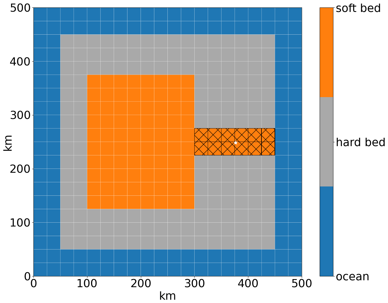
Figure 1 Modified ISMIP–HEINO geometry (Calov and Greve, 2006). The model domain is reduced to 500×500 km to enable horizontal grid resolutions up to 3.125 km. The shown grid resolution is 25×25 km. The basal topography is flat, and the hatched area marks the soft-bedded pseudo-Hudson Strait. The white star indicates the location of the grid cell shown in Figs. 8 and S21.

While Mantelli et al. (2019) conclude that Stokes mechanics are needed to arrive at a mathematically well-posed model, running numerical experiments with a thermo-mechanically coupled Stokes model is currently unfeasible over glacial-cycle timescales. Previous ice stream surge modeling studies are often based on zeroth-order, thin-film approximations of the Stokes problem, like the shallow-ice approximation (SIA, e.g., eight out of nine models in the ISMIP–HEINO experiments – Calov et al., 2010). While resolving vertical shear, which is the dominant mode of motion in slow-flowing regions, SIA-based models neglect longitudinal stress gradients and horizontal shear, which are known to be important for fast ice streams (Hindmarsh, 2009) and are instead captured by the zeroth-order shallow-shelf approximation (SSA).

To partially offset the limitations of the zeroth-order approximations, the GSM uses hybrid SIA–SSA ice dynamics (Pollard and DeConto, 2007, 2012). The hybrid SIA–SSA ice dynamics are activated for grid cells with an SIA velocity exceeding 30 m yr⁻¹. Changing these activation velocities (20 and 40 m yr⁻¹) has no significant effect on the surge characteristics (Table S1 in the Supplement). Activating the SSA everywhere leads to more surges that are also shorter and weaker because no threshold velocity needs to be overcome to initiate basal sliding (Sect. S1.2). Note that we set an upper limit of 40 km yr⁻¹ for the SSA velocity to ensure that sliding velocities stay within a physically reasonable range.

We configure the GSM with a 1 km deep (17 non-linearly-spaced levels) bed thermal model. A basal-temperature ramp is used to ensure a smooth transition between cold-based regions of no sliding and temperate sliding, to account for observational evidence of sub-temperate sliding, and to more accurately represent the sub-grid warm-based ice fraction in a grid cell and therefore more accurately represent sliding onset for coarse grid resolutions (Q₅ in Sect. 1.3). However, the shape of such a basal-temperature ramp is not well constrained. In the GSM, the basal-temperature ramp is incorporated into a Weertman-type power law,

$$\begin{array}{}\text{(6a)}& {\mathit{u}}_{\mathrm{b}}=C_{\mathrm{b}}{\left|{\mathit{\tau }}_{\mathrm{b}}\right|}^{n_{\mathrm{b}}-\mathrm{1}}{\mathit{\tau }}_{\mathrm{b}},\end{array}$$

as a dependence of the basal-sliding coefficient C_b on the estimated warm-based fraction of a grid cell (indirectly accounting for sub-temperate sliding) F_warm (Eq. 8):

$$\begin{array}{}\text{(6b)}& C_{\mathrm{b}}=\left(\mathrm{1}-F_{\mathrm{warm}}\right)C_{\mathrm{froz}}+F_{\mathrm{warm}}C,\end{array}$$

where u_b is the basal-sliding velocity, τ_b is the basal stress, n_b is the bed power strength (Table 1), and C is the fully warm-based sliding coefficient (depending on the bed properties; see also Fig. S4). C_froz is the fully cold-based sliding coefficient for numerical regularization:

$$\begin{array}{}\text{(7)}& C_{\mathrm{froz}}=\mathrm{2}\times {\mathrm{10}}^{-\mathrm{3}}\mathrm{m}{\mathrm{yr}}^{-\mathrm{1}}{\left(\mathrm{5}\times {\mathrm{10}}^{-\mathrm{6}}{\mathrm{Pa}}^{-\mathrm{1}}\right)}^{n_{\mathrm{b}}}.\end{array}$$

F_warm is calculated according to

$$\begin{array}{}\text{(8)}& F_{\mathrm{warm}}=\max {\left[\mathrm{0},\min \left(\mathrm{1},{\displaystyle \frac{T_{\mathrm{bp},\mathrm{I}}+T_{\mathrm{ramp}}}{T_{\mathrm{ramp}}}}\right)\right]}^{T_{\exp }},\end{array}$$

where T_bp,I is the grid cell interface basal temperature relative to the pressure-melting point, negative T_ramp is the temperature below which the entire grid cell is cold-based, and T_exp is the exponent used for the ramp. The values used in previous GSM modeling studies (T_ramp=1.0 ^∘C and T_exp=28 – e.g., Bahadory and Tarasov, 2018) were based on horizontal basal-temperature gradients around the basal-sliding activation zone, with consideration of the sub-grid warm-based connectivity between grid cell interfaces (as basal sliding requires a connected sub-grid warm-based path). Different values for T_ramp and T_exp are explored within this paper. T_ramp can be chosen as either a constant or depending on the horizontal grid resolution (res – equal extent in x and y directions):

$$\begin{array}{}\text{(9)}& T_{\mathrm{ramp}}=P_{T_{\mathrm{ramp}}}\cdot {\displaystyle \frac{\mathrm{res}}{\mathrm{50}\mathrm{km}}}{}^{\circ }\mathrm{C}.\end{array}$$

This choice of resolution dependence leads to a sharper temperature ramp for finer horizontal grid resolutions. The parameter $P_{T_{\mathrm{ramp}}}$ is used to conduct experiments with different temperature ramps at the same horizontal grid resolution (Sect. 3.3.3). The temperature ramps for all four horizontal grid resolutions and $P_{T_{\mathrm{ramp}}}=\mathrm{1}$ (default value) are shown in Fig. 2. For comparison, a temperature ramp similar to the one suggested by Fowler (1986) and later by Mantelli et al. (2019),

$$\begin{array}{}\text{(10)}& F_{\mathrm{warm}}=\exp \left({\displaystyle \frac{T_{\mathrm{bp},\mathrm{I}}}{\mathit{\delta }}}\right)\mathrm{for}{T}_{\mathrm{bp},\mathrm{I}}\le \mathrm{0},\end{array}$$

is shown for δ=0.01, where δ is a parameter controlling the width of the transition zone. Based on experiments conducted by Barnes et al. (1971), Mantelli et al. (2019) expect δ to be small.

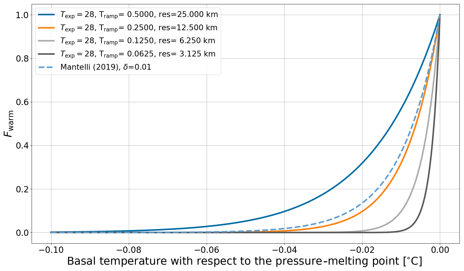
Figure 2 Temperature ramps for different values of T_ramp which depend on the horizontal grid resolution. A temperature ramp similar to the one suggested by Mantelli et al. (2019) (Eq. 10) is shown for δ=0.01.

2.1.2 GSM ensemble input parameter vectors

Each GSM experiment is run with an ensemble based on five input parameter vectors. The current idealized setup encompasses a maximum of eight input parameters (Table 1) per parameter vector. The five parameter vectors used in this study are hand-picked from an exploratory ensemble (Fig. S3). The criteria for these five parameter vectors were the highest subset variance in surge characteristics and the soft-bed sliding-law exponent. Note that the soft- and hard-bed sliding-law exponents in this study are equal (n_b in Table 1). Due to the significantly increased model run time, sliding-law exponents larger than 3 are not considered here. To isolate interactions, the GSM reference setup used in this paper does not incorporate basal hydrology and glacial isostatic adjustment (GIA). Processes associated with basal hydrology, such as lubrication of the bed and decoupling of the ice sheet from the bed, are likely to have a major effect on surge patterns. To determine the impact of these effects, we run the GSM with local basal hydrology enabled (Eqs. 19 to 21, Sect. 3.3.5) and examine resolution scaling (Sect. S9.2). However, experiments done with and without basal hydrology lead to qualitatively similar results (e.g., same conclusions from upscaling experiments in Sect. 3.3.3). We therefore omit sub-glacial hydrology coupling for the main analysis.

Table 1 Model parameters are listed with respect to their purpose or category. Ice sheet model – ISM. Hydrology parameters used when running the GSM with local basal hydrology. Additional (non-regular) input parameters that are usually set to a fixed value. The default values of the 3.125 km horizontal grid resolution reference setup are shown as bold values (in brackets) for the additional parameters.

2.1.3 GSM model setups

The reference setup (Table 2) has a 3.125 km horizontal grid resolution and a 1-year maximum time step size. The bed topography is flat (at sea level), and an asymmetric temperature forcing is used (Fig. S1). For the sake of generality, we chose a flat topography for the reference setup, while the effect of a basal trough is investigated at a later stage (Sect. 3.3.4). Branching off this reference setup, we carry out one-factor-at-a-time sensitivity experiments to isolate numerical and process impacts. These experiments, in turn, examine the response to three numerical aspects related to the MNEEs, four model aspects affecting the thermal onset of basal sliding, a change in sediment cover, a non-flat topography, the addition of local basal hydrology, and different horizontal grid resolutions (25, 12.5, 6.25 km). The three numerical aspects are stricter numerical convergence criteria, the addition of surface temperature noise (±0.1 and ±0.5 ^∘C), and an approximate implicit time step coupling between the thermodynamics and ice dynamics. The four thermal model aspects are switching to a thin (20 m)-bed thermal model, different approaches to determining the basal temperature at the grid cell interface, different weights of the adjacent minimum basal temperature for the basal-sliding temperature ramp (W_Tb,min), and different basal-temperature ramps (T_ramp and T_exp) for thermal activation of basal sliding. See Table 1 for details on parameter ranges.

2.2 PISM

2.2.1 PISM model description

In contrast to the GSM, the Parallel Ice Sheet Model (PISM) is not specifically developed for glacial-cycle ensemble modeling. Therefore, the two models use distinct sets of numerical optimizations for computational speed. To minimize the model dependency of our analysis, experiments are also carried out with v2.0.2 of PISM.

Similarly to the GSM, PISM is a 3D thermodynamically coupled ice sheet model, and the SSA is used as a sliding law once the sliding velocity exceeds 100 m yr⁻¹. For further details on the model itself, refer to Bueler and Brown (2009) and Winkelmann et al. (2011). The details on the default PISM setup, together with the default GSM values, are listed in Table 2. Given the higher computational cost of PISM experiments, the relatively high sensitivity of PISM to the number of parallelized cores for these experiments (Table 6), and the run time limitations of the computational cluster, the reference setup is run at 25 km horizontal grid resolution.

For stability reasons, the PISM adaptive time-stepping ratio (used in the explicit scheme for the mass balance equation) was reduced to 0.01 when using small till friction angles (Constantine Khrulev, personal communication, 26 May 2021).

The default sliding law in PISM is a purely plastic (Coulomb) model, where

$$\begin{array}{}\text{(11)}& \left|{\mathit{\tau }}_{\mathrm{b}}\right|\le {\mathit{\tau }}_{\mathrm{c}}\mathrm{and}{\mathit{\tau }}_{\mathrm{b}}=-{\mathit{\tau }}_{\mathrm{c}}{\displaystyle \frac{\mathit{u}}{\left|\mathit{u}\right|}}\mathrm{if}\left|\mathit{u}\right|>\mathrm{0}.\end{array}$$

Therefore, the basal-shear stress τ_b can never exceed the yield stress τ_c, and basal sliding only occurs when τ_b reaches τ_c.

(Tulaczyk et al., 2000a)

Table 2 Comparison between the GSM and PISM reference setup.

2.2.2 PISM ensemble input parameter vectors

The PISM configuration encompasses six model input parameters (Table 3). These parameters define the input fields for surface temperature, surface accumulation, and till friction angle. As for the GSM, PISM is initialized from ice-free conditions. Similarly to Calov and Greve (2006), the surface temperature at every grid cell is calculated as follows:

$$\begin{array}{}\text{(12)}& T_{\mathrm{surf}}=T_{\min }+S_{\mathrm{t}}\cdot d^{\mathrm{3}},\end{array}$$

where S_t represents the horizontal surface temperature gradient; d represents the distance from the domain center (x_center, y_center) in kilometers, defined as

$$\begin{array}{}\text{(13)}& d=\sqrt{(x-x_{\mathrm{center}}{)}^{\mathrm{2}}+(y-y_{\mathrm{center}}{)}^{\mathrm{2}}}<R;\end{array}$$

and R denotes the radius and sets an upper limit for d. A comparable equation is used to calculate the surface mass balance (accumulation–ablation) rate input field:

$$\begin{array}{}\text{(14)}& B_{\mathrm{surf}}=B_{\max }-S_{\mathrm{b}}\cdot d^{\mathrm{5}},\end{array}$$

where S_b is the horizontal surface mass balance gradient. The input field for the till friction angle is defined by simple grid assignment and a somewhat smoothed transition between the soft- and hard-bed region. Input fields for one parameter vector are shown for surface temperature, surface accumulation, and till friction angle in Figs. S6, S7, and S8, respectively.

Table 3 Parameters used to generate the PISM input fields.

The 6 model ensemble parameters (Table 3) were selected via Latin hypercube sampling. After sieving an ensemble of 100 runs for those that show oscillatory behavior, a nine-member high-variance (with respect to the surge characteristics) subset was extracted by means of visual identification (Fig. S10). Each PISM experiment is run with an ensemble based on these nine input parameter vectors.

2.2.3 PISM bed properties

A PISM ensemble parameter restriction arose as experiments carried out with PISM only show oscillatory behavior for small yield stresses τ_c. This can be achieved by means of either a small till friction angle Φ or a low effective pressure on the till (N_till, Eq. S2) (Bueler and Van Pelt, 2015):

$$\begin{array}{}\text{(15)}& {\mathit{\tau }}_{\mathrm{c}}=c_{\mathrm{0}}+\tan \left(\mathrm{\Phi }\right)N_{\mathrm{till}},\end{array}$$

where c₀=0 Pa is the till cohesion (Tulaczyk et al., 2000b). For convenience, we decide to vary only the till friction angle between 0.5 and 1^∘, for which PISM shows oscillatory behavior; otherwise, we use PISM default values (see Sect. S2.3 for details).

The resulting very slippery beds enabled occasional maximum sliding velocities of up to ∼600 km yr⁻¹ in the simulations (Fig. S11, Sect. S2.4). For comparison, observed outlet glacier velocities at Jakobshavn Isbræ(Greenland) approach 20 km yr⁻¹ (Joughin et al., 2012, 2014). As for the GSM, we, therefore, set an upper limit of 40 km yr⁻¹ for the SSA velocity.

2.2.4 PISM model setups

As for the GSM, we carry out one-factor-at-a-time sensitivity experiments branching off the PISM reference setup (Table 2) for all nine parameter vectors. These experiments, in turn, examine the response to two numerical aspects related to the MNEEs, removing the bed thermal model, an abrupt sediment transition zone, a non-flat topography (Fig. S9), a mass-conserving horizontal transport model for basal hydrology (Bueler and Van Pelt, 2015), and different horizontal grid resolutions (50, 12.5 km). The two numerical aspects are different number of processor cores ($n=\mathrm{2},\mathrm{4},\mathrm{16},\mathrm{32}$) and the addition of surface temperature noise (±0.1 and ±0.5 ^∘C).

2.3 Run analysis approach

2.3.1 Surge characteristics

The quantities being analyzed are the number of surges, the surge duration, the ice volume change during a surge, and the period between surges (Fig. 3). The surge time is defined as the time of minimum (pseudo-Hudson Strait) ice volume, and the duration of a surge includes the surge itself, as well as the time it takes the ice sheet to recover approximately half the ice volume lost during the surge (Sect. S3). The calculated ice volume change is the difference between the pre-surge and minimum (pseudo-Hudson Strait) ice volume in that particular surge (Sect. S3). The period between surges is the time span between two subsequent occurrences of minimum (pseudo-Hudson Strait) ice volume (not defined for the very last surge). The spin-up interval (first 20 kyr of every run) is not incorporated in the analysis, and only surges with a (pseudo-Hudson Strait) ice volume change of more than 500 and 4×10⁴ km³ are considered in the GSM and PISM analyses, respectively (∼5 % of mean ice volume across all runs). Note that this is a very conservative spin-up interval. For example, most GSM runs reach their mean pseudo-Hudson Strait ice volume after ∼5 kyr (e.g., Fig. 11).

Figure 3 Pseudo-Hudson Strait ice volume of a GSM model run with visual illustration of the surge characteristics used to compare different model setups. The horizontal grid resolution is 3.125 km.

In addition to the surge characteristics, the root mean square error (RMSE) and mean bias are calculated as a percentage deviation from the reference (pseudo-Hudson Strait) ice volume time series for all setups (each parameter individually) and are then averaged over the five parameter vectors (Eqs. S3 and S4). The full run time is considered (no spin-up interval).

2.3.2 Percentage differences

We compare different model setups by calculating the percentage difference between the reference setup and all other setups for every parameter vector individually and then average this difference over all parameter vectors. Crashed runs are not considered, and runs with less than two surges require special treatment (see Sect. S5 for further details on the analysis).

2.3.3 Surge area

In the GSM, the whole pseudo-Hudson Strait (Fig. 1) is ice covered and at maximum ice volume at the beginning of a surge. Surges in the GSM, therefore, consistently appear as ice volume minima, which allows us to directly use the pseudo-Hudson Strait ice volume for the GSM results.

For PISM, a large fraction of the pseudo-Hudson Strait area is only ice covered when a surge occurs (e.g., Fig. 5), leading to an inconsistency in the surge detection. This issue is addressed by including the ice volume over the eastern half of the pseudo-Hudson Bay, the area most affected by the surge drained through the pseudo-Hudson Strait. See Sect. 2.5 for further details and a comparison between the two approaches.

2.3.4 Minimum numerical error estimates

We compute the new minimum numerical error estimates (MNEEs) threshold by examining the model response to changes in the model configuration that are not part of the physical system. The MNEEs are defined as the percentage differences in surge characteristics when applying a stricter (than default) numerical convergence in the GSM and changing the number of processor cores used in PISM. The differences between PISM runs with different numbers of processor cores can be caused by, for example, a different order of floating-point arithmetic operations and the processor-number-dependent preconditioner used in PISM (PISM 2.0.6 documentation, 2023). The MNEEs are then used as a threshold to determine if model sensitivities to changes in the model configuration that affect the physical system (e.g., the inclusion of a bed thermal model or sliding dependence on effective pressure from basal hydrology) are above the numerical errors induced by iterative numerical solvers in the model. We refrain from drawing conclusions about the effects of a change in model configuration with physical relevance when the model sensitivities in question are smaller than the MNEEs. In these cases, the actual physical response of the model might be hidden within the numerics.

While the MNEEs are useful for our purpose, we wish to emphasize that they can not replace proper model verification and validation and are missing uncertainties due to, e.g., different approximations of the Stokes equations and other physical processes not included in the models. Nonetheless, they provide a minimum estimate of the numerical model error, which is still a significant improvement over ignoring this issue entirely.

3 Results

3.1 Key surge characteristics of the reference setup

Before analyzing ensemble characteristics, it is crucial to understand how surges initiate, propagate, and terminate. Surges in the GSM originate at the pseudo-Hudson Strait mouth (x=450 km, y=225 to 275 km) and propagate towards the center of the pseudo-Hudson Bay (x=200 km, y=250 km – Figs. 1 and 4). The surging onset is a complex interplay between heating at the ice sheet bed, basal temperature, and ice sheet velocity. The beginning of a surge is shown in video 01 (Hank, 2023) and Fig. 4. Just before the start of the surge, the entire south–north extent of pseudo-Hudson Strait grid cells close to the ocean is warm based. At t=6.69 kyr, the SIA velocities exceed 30 m yr⁻¹, and the SSA is activated (Sect. 2.1.1). The longitudinal stress gradient and horizontal shear terms provide additional heating. This leads to several small ice streams with relatively strong heating due to basal sliding (∼10⁷ J m⁻² yr⁻¹) at t=6.70 kyr in the video. This is 1 order of magnitude larger than heat production from deformation work. The additional heat fosters higher ice velocities, leading to even more heating, the extension of the warm-based area to the west, and therefore the upstream propagation of the small ice streams (t=6.71 kyr). The narrow ice streams draw in warm-based ice from the surrounding grid cells, increasing the velocities and heat production in the area between the ice streams. This leads to a merger of the ice streams with now high velocities occurring over the full south–north extent of the pseudo-Hudson Strait (t=6.72 kyr). The warm-based area rapidly extends towards the west due to the strong heating and high ice velocities, causing a pseudo-Hudson Strait surge.

Figure 4 Basal-ice velocity for parameter vector 1 at different time steps using the GSM. The horizontal grid resolution is 3.125 km, and the maximum model time step is 1 year. The contour lines show the ice sheet surface elevation in meters. The magenta line outlines the soft-bedded pseudo-Hudson Bay and Hudson Strait. Note that the top and bottom rows show different areas of the domain, with the top zooming in on the surge onset area.

The surge propagates nearly symmetrically until the pseudo-Hudson Bay area is reached (t=6.77 kyr in Fig. 4 and video 02 of Hank, 2023). After this point, the northern branch of the ice stream propagates more rapidly and extends further to the west than the southern branch. While the smaller southern branch starts to shrink at t=6.81 kyr, the northern part propagates until t=6.83 kyr. At this time, the southern branch vanishes almost completely due to a thinner ice sheet (than at the start of the surge) and the advection of cold ice into the surge area. After t=6.83 kyr, the available heating is no longer sufficient to keep the ice sheet bed at the pressure-melting point, and the northern part collapses as well. The surge ends after 150 years (at t=6.87 kyr).

Since the GSM setup and climate forcing are symmetric about the horizontal axis in the middle of the pseudo-Hudson Strait (y=250 km in Fig. 1), we interpret the induced asymmetry to be “spontaneous symmetry breaking”, similarly to the results described in Sayag and Tziperman (2011). We define the asymmetry as positive when the surge is stronger northward (Fig. 4 and video 02 of Hank, 2023) or shifted northward. The asymmetry sign varies across the first surges (i.e., the surge least biased by previous asymmetries) of the five reference runs, ruling out any persistent numerical bias.

Figure 5 Basal-ice velocity for parameter vector 8 at different time steps using PISM. The horizontal grid resolution is 25 km, and the maximum model time step size is 1 year. Otherwise as in Fig. 4.

Surges in PISM originate at the ice sheet margin in the soft-bedded pseudo-Hudson Strait (exact position varies between runs) and propagate towards the center of the pseudo-Hudson Bay (x=1300 km, y=1500 km – Figs. S8 and 5). The ice near the margin is already flowing downstream before the start of the surge (t=89.36 kyr). However, the basal temperature is below the pressure-melting point, and the ice velocities are low (<100 m yr⁻¹). As the ice sheet upstream of the margin thickens, the warm-based area extends further downstream, particularly along the 100 % soft-bedded contour line (magenta line in Fig. 5).

Once the warm-based area connects with the margin (t=89.42 kyr), the ice velocities increase beyond 100 m yr⁻¹, activating the SSA (Sect. 2.2.1). Similarly to the surges in the GSM, the sliding velocities then increase rapidly, quickly extending the warm-based area (t=89.43 and t=89.433 kyr). The surge propagates upstream into the pseudo-Hudson Bay, and the ice is transported along the pseudo-Hudson Strait into regions with increasingly negative surface mass balance rates (t=89.435 to t=89.45 kyr, Fig. S7). The ice sheet thins; the basal temperature at the margin falls below the pressure-melting point, blocking parts of the upstream ice stream; and the surge ceases at t=89.47 kyr (∼100 year surge duration). The ice volume in the surge-affected area continues to decrease for, on average, another 2.5 kyr due to the large amounts of ice in the negative surface mass balance regions. In contrast to the GSM, PISM results remain symmetrical at about y=1500 km throughout the surge.

Due to the differences in model setups, physics, and numerics (Table 2), the GSM and PISM reference setups yield different surge characteristics (Table 4). While resembling the inferred ice-rafted debris (IRD) interval duration as closely as possible is not a goal of this study, the modeled values are in agreement with the literature (200 to 2280 years, Hemming, 2004). The mean modeled GSM period is shorter than the observed period of, on average, 7 kyr (Cuffey and Paterson, 2010). However, exploratory GSM runs with a dimensionally accurate (not downscaled) model domain (but otherwise identical experimental setup) yielded periods within the range of geological inferences. The mean modeled PISM period is within limits set by the literature. The mean (pseudo-Hudson Strait) ice volume change in the GSM corresponds to 15 % of a 1.5 km thick ice sheet covering the downscaled pseudo-Hudson Strait area (150×50 km). In PISM, the mean ice volume change is 7.1 % of the mean (across reference setup runs) maximum ice volume in the eastern half of the pseudo-Hudson Bay and pseudo-Hudson Strait.

Table 4 Surge characteristics of the GSM (T_ramp=0.0625 ^∘C, T_exp=28 (black line in Fig. 2), $W_{\mathrm{Tb},\min }=\mathrm{0.5}$, TpmTrans for the interface calculation, sharp transition between hard and soft bed) and PISM reference setup (Table 2). No runs crashed, and all runs had more than one surge. The first 20 kyr of each run are treated as a spin-up interval and are not considered in the above.

3.2 Minimum numerical error estimates

Differences in surge characteristics (compared to the reference setup) are considered to be significant when they exceed the MNEEs given in Tables 5 and 6 for the GSM and PISM, respectively. However, this does not necessarily mean that smaller changes have no physical relevance but rather that their interpretation is difficult (if not impossible) because the physical response is hidden within the numerical sensitivities. Likely sources of the MNEEs are the iterative SSA solutions and floating-point accuracy.

To determine a minimum significant threshold in the GSM, we re-run a set of GSM runs with 3.125 km horizontal grid resolution, imposing a stricter numerical convergence (decreasing final iteration thresholds). In a second experiment, we additionally increase the maximum iterations from two to three for the outer Picard loop solving for the ice thickness and from two to four when solving the non-linear elliptic SSA equation for horizontal ice velocities.

The largest differences between simulations occur for the mean period (7 %, Table 5) when using stricter convergence thresholds (no change in the maximum number of iterations). The standard deviations are of the same order of magnitude as the values themselves, indicating different responses across the five parameter vectors. Determining the MNEEs at 12.5 km instead of 3.125 km horizontal grid resolution yields similar results, except for the mean pseudo-Hudson Strait ice volume change (21 %, Table S2).

Table 5 Percentage differences (except first column) of surge characteristics between GSM runs with regular and stricter numerical convergence and increased maximum iterations for the ice dynamics loops at 3.125 km horizontal grid resolution. The values represent the averages of five parameter vectors. No runs crashed, and all runs had more than one surge. The first 20 kyr of each run are treated as a spin-up interval and are not considered in the above. The bold numbers mark the largest MNEE for each surge characteristic.

MNEEs in PISM are determined by comparing runs with different numbers of cores. Although most parameter vectors show similar results at the beginning of the runs, minor differences can slowly accumulate and lead to significant discrepancies in surge activity by the end of the run (Fig. S18). The largest differences occur for the number of surges (16 %) and mean ice volume change (16 %) for nCores =32, but the standard deviations are large due to a more than ∼200 % increase in both surge characteristics for parameter vector 6.

Table 6 Percentage differences of surge characteristics (except first row) between the PISM reference setup and setups with different numbers of cores at 25 km horizontal grid resolution. The values represent the averages of nine parameter vectors. No runs crashed, and all runs showed at least one surge. Runs with just one surge (nS1) are ignored when calculating the change in mean period. The first 20 kyr of each run are treated as a spin-up interval and are not considered in the above. The bold numbers mark the largest MNEE for each surge characteristic.

The differences in surge characteristics between different numbers of cores can be minimized (but not removed entirely) by decreasing the relative Picard tolerance in the calculation of the vertically averaged effective viscosity (10⁻⁴ to 10⁻⁷) and the relative tolerance for the Krylov linear solver used at each Picard iteration (10⁻⁷ to 10⁻¹² – Table S5 and Fig. S19). However, this leads to an unreasonable increase in model run time (∼300 %) that is not feasible for an ensemble-based approach (more than 50 % of all runs did not finish within the time limit of the computational cluster). Intermediate decreases in the relative tolerances still lead to significant differences in surge characteristics while increasing the model run time and are, therefore, not used in the PISM reference setup. Considering that small differences prevail for all tested relative tolerances, comparing model configurations with different numbers of cores for, e.g., finer-horizontal-grid-resolution experiments is not straightforward.

3.2.1 Adding surface temperature noise

Low levels of surface temperature noise have previously been shown to cause chaotic behavior in the mean periods of oscillations (Souček and Martinec, 2011). Adding low levels of uniformly distributed surface temperature noise (maximum amplitude of ±0.1 and ±0.5 ^∘C) to the climate forcing (updated every 100 years) does not significantly affect the surge characteristics for the GSM (Table S3). For example, the effect of adding ±0.5 ^∘C surface temperature noise on the mean period is only 4 % (compared to the ∼20 % for ±0.01 ^∘C reported by Souček and Martinec, 2011). Adding the same levels of uniformly distributed surface temperature noise to PISM increases the mean duration by 12 % (for ±0.1 ^∘C) but has no significant effect on the other surge characteristics (Table S6).

3.2.2 Implicit thermodynamics–ice-dynamics coupling

In contrast to the commonly used explicit time step coupling between the thermodynamics and ice dynamics in glaciological ice sheet models, we test the impact of approximate implicit time step coupling via an iteration between the two calculations for each time step. The implicit coupling decreases the mean duration and pseudo-Hudson Strait ice volume change (−13 % and −25 %, respectively). The number of surges and mean period show no significant change (Table S4). While the changes in mean duration and pseudo-Hudson Strait ice volume change are larger than the MNEEs, they do not justify an increase in run time of ∼265 %, and the implicit coupling is therefore omitted for the GSM reference setup.

3.3 Sensitivity experiments

Here, we discuss differences in surge characteristics due to changes in the model setup. An overview of the results can be found in Figs. 6 and 7 for the GSM and PISM, respectively. The exact values of the percentage differences are provided in the Supplement. We first examine the model aspects affecting the thermal activation of basal sliding (Sect. 3.3.1 to 3.3.3), followed by the analysis of a smooth sediment transition zone, non-flat topography, and local basal hydrology (Sect. 3.3.4 and 3.3.5). Experiments without significant differences in the surge characteristics are only briefly mentioned here (Sect. 3.3.6). A more in-depth discussion of these latter experiments is available in the Supplement.

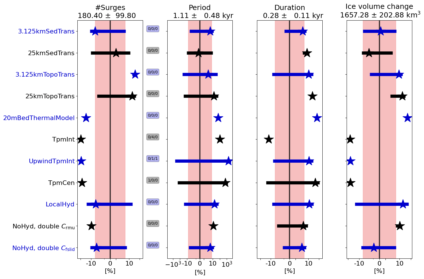
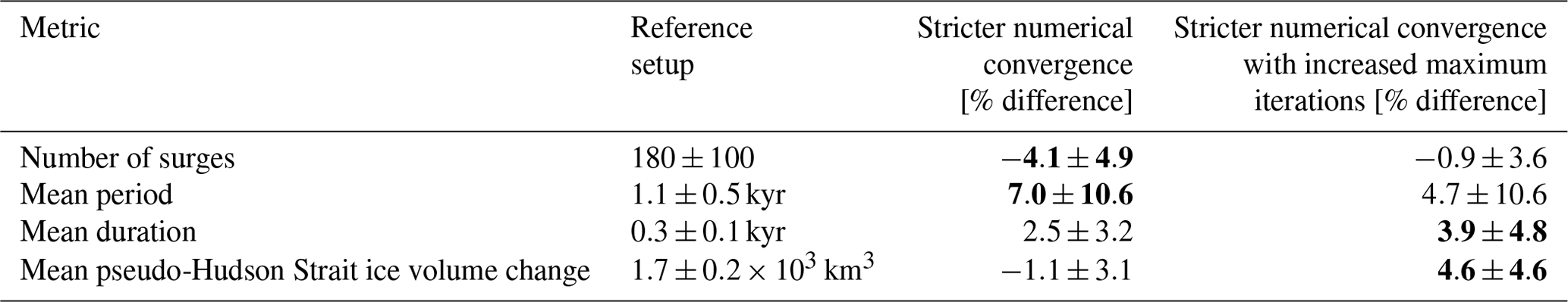
Figure 6 Percentage differences in surge characteristics compared to the GSM reference setup for model setups discussed in Sect. 3.3 (average of the five parameter vectors). The horizontal grid resolution is 3.125 km. The different colors were added for visual alignment of the individual model setups, the stars are the ensemble mean percentage differences, and the horizontal bars represent the ensemble standard deviations. The shaded pink regions mark the MNEEs (Table 5), and the black numbers in the title of each subplot represent the mean values of the reference setup. The three small numbers between the first two columns represent the number of crashed runs (nC), the number of runs without a surge (nS0), and the number of runs with only one surge (nS1). The first 20 kyr of each run are treated as a spin-up interval and are not considered in the above. The x axis is logarithmic. Further details of each individual experiment are provided in the subsequent sections and the Supplement. The model setups, from top to bottom, are as follows: 3.125 km wide sediment transition zone (instead of an abrupt transition in the reference setup), 25 km wide sediment transition zone, 3.125 km wide sediment transition zone with pseudo-Hudson Bay and Hudson Strait topography (instead of a flat topography in the reference setup), 25 km sediment transition zone with pseudo-Hudson Bay and Hudson Strait topography, 20 m deep (one layer) bed thermal model (instead of a 1 km deep bed thermal model (17 non-linearly spaced layers) in the reference setup), three different approaches to calculate basal grid cell interface temperature (TpmInt, upwind TpmInt, TpmCen), local hydrology (instead of no hydrology), and doubling the values of the soft- and hard-bed sliding coefficients (as an attempt to represent basal hydrology without actually adding it).

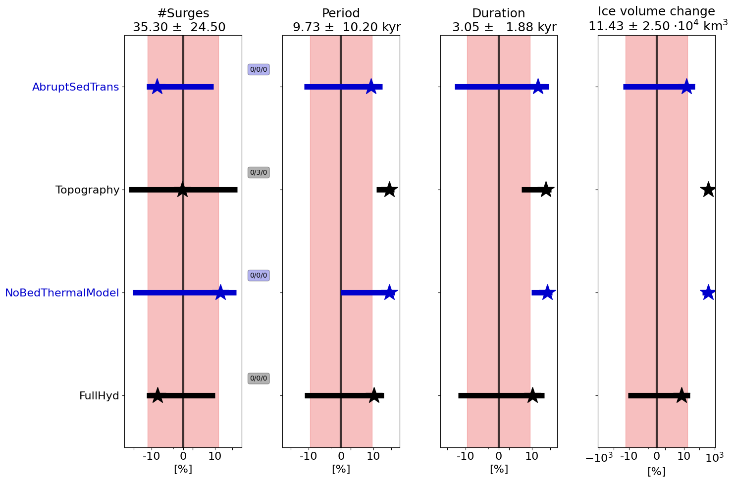
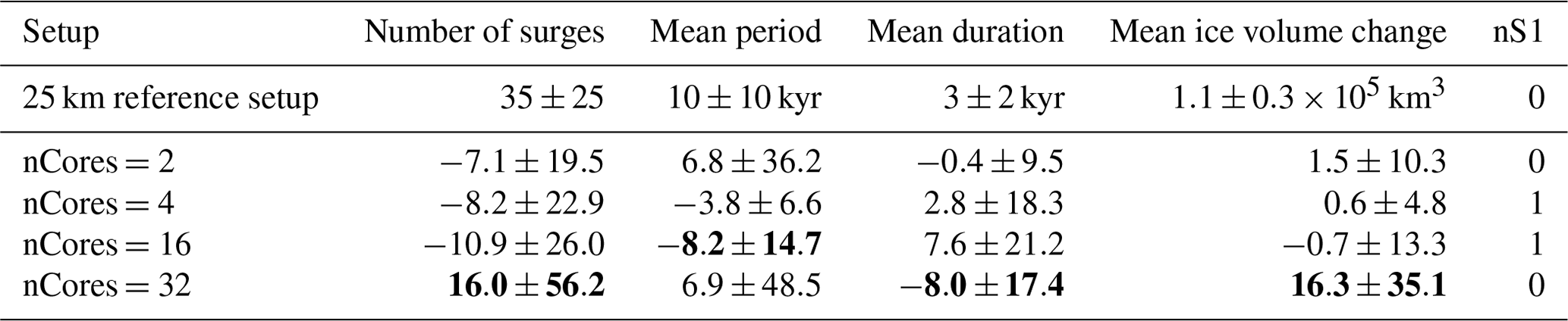
Figure 7 Percentage differences in surge characteristics compared to the PISM reference setup for model setups discussed in Sect. 3.3 (average of the nine parameter vectors). The horizontal grid resolution is 25 km. Otherwise same as Fig. 6. The model setups, from top to bottom, are as follows: abrupt sediment transition (instead of the transition shown in, e.g., Fig. S8), pseudo-Hudson Bay and Hudson Strait topography (instead of a flat topography in the reference setup, Fig. S9), no bed thermal model (instead of a 1 km deep bed thermal model (20 equally spaced layers) in the reference setup), and a mass-conserving horizontal transport model for basal hydrology (instead of a local hydrology).

3.3.1 Bed thermal model

First, we examine the effects of a 1 km deep bed thermal model on the basal temperature and the surge characteristics in the GSM and PISM. Both models show significant differences when limiting the bed thermal model to one layer (GSM) or when removing it entirely (PISM).

Advection of cold ice near the end of a surge rapidly decreases the basal-ice temperature and, therefore, increases the temperature gradient between the basal ice and the bed. In GSM runs with the 1 km deep (17 non-linearly spaced levels) bed thermal model (reference setup), this stronger gradient increases the heat flux from the bed into the ice and dampens the actual change in basal-ice temperature. Similarly, a rapid increase in basal-ice temperature due to higher basal-ice velocities at the beginning of a surge reverses the existing temperature gradient at the base of the ice sheet, leading to a heat flux from the ice into the bed. Consequently, less heat is available to warm the surrounding cold-based ice, counteracting the surge propagation (Fig. 8).

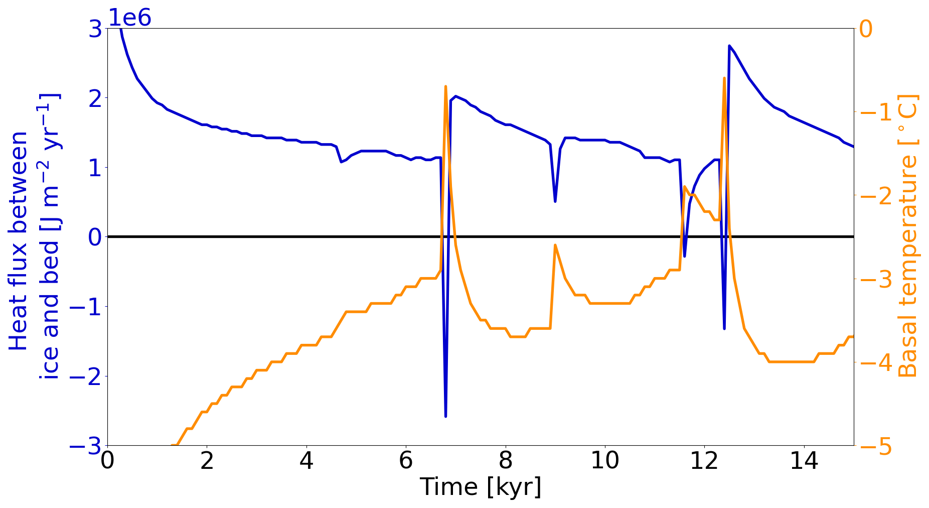
Figure 8 Heat flux at the base of the ice sheet (positive from bed into ice) and basal-ice temperature for a grid cell in the center of the pseudo-Hudson Strait (grid cell center at x=376.5625 and y=248.4375 km, white star in Fig. 1) and parameter vector 1 with the 1 km deep bed thermal model (17 non-linearly spaced levels) using the GSM. The horizontal grid resolution is 3.125 km.

With only one bed thermal layer (20 m deep, removing most of the heat storage), the variance of the average basal temperature with respect to the pressure-melting point in the pseudo-Hudson Strait increases (Fig. S20), and more heat is available to warm the surrounding ice (no or smaller heat flux into the bed, Fig. S21). The additional heat increases the mean pseudo-Hudson Strait ice volume change and duration (50 % and 65 %, respectively – Fig. 6). Due to the larger changes in pseudo-Hudson Strait ice volume and average basal temperature with respect to the pressure-melting point, the ice sheet requires more time to reach the pre-surge state when only one bed thermal layer is used. Therefore, the period increases (60 %), while the number of surges drops. These differences in surge characteristics exceed the MNEEs (Table 5). The stronger surges (larger pseudo-Hudson Strait ice volume change) lead to overall less ice volume in the pseudo-Hudson Strait (Table S7). Running PISM without the 1 km deep (20 equally spaced levels) bed thermal model yields similar behavior to the GSM, further underlining the impact of a bed thermal model. The mean period, mean duration, and mean ice volume change all increase (80 %, 70 %, and 396 %, respectively – Fig. 7). In contrast to the GSM characteristics, the number of surges increases for runs without a bed thermal model. However, the standard deviation is large, and the change in the number of surges is somewhat misleading. The number of surges decreases for six out of nine runs. Parameter vectors showing an increase in the number of surges without a bed thermal model show very few surges (e.g., Fig. S22) or transition to a constantly active ice stream when the bed thermal model is included. As for the GSM, the stronger surges lead to an overall smaller ice sheet in the surge-affected area (Table S8).

3.3.2 Basal temperature at the grid cell interface

Another modeling choice that affects the thermal activation of basal sliding is the approach to determining the basal temperature at the grid cell interface. The most straightforward approach to determining the basal temperature with respect to the pressure-melting point at the grid cell interface (T_bp,I) is to use the mean of the two adjacent basal temperatures with respect to the pressure-melting point at the grid cell centers (TpmCen):

$$\begin{array}{}\text{(16)}& T_{\mathrm{bp},\mathrm{I}}=\mathrm{0.5}\cdot \left(T_{\mathrm{bp},\mathrm{L}}+T_{\mathrm{bp},\mathrm{R}}\right),\end{array}$$

where T_bp,L and T_bp,R are the grid cell center basal temperatures with respect to the pressure-melting point to the left and right of the interface, respectively. This is similarly the case for upper and lower grid cells adjacent to a horizontally aligned interface. However, this approach does not explicitly account for ice thickness changes at the grid cell interface.

TpmInt, on the other hand, calculates the basal temperature at the interface (T_I) by averaging the adjacent grid cell center basal temperatures (T_L and T_R, Eq. 17a). T_bp,I is then determined by using the interface ice sheet thickness (average of adjacent grid cell center ice thicknesses H_L and H_R, Eq. 17b):

$$\begin{array}{}\text{(17a)}& {\displaystyle }{T}_{\mathrm{I}}=\mathrm{0.5}\cdot \left(T_{\mathrm{L}}+T_{\mathrm{R}}\right),\text{(17b)}& {\displaystyle }{T}_{\mathrm{bp},\mathrm{I}}=T_{\mathrm{I}}+{\mathit{\beta }}_{\mathrm{P}}{\displaystyle \frac{H_{\mathrm{L}}+H_{\mathrm{R}}}{\mathrm{2}}},\end{array}$$

where ${\mathit{\beta }}_{\mathrm{P}}=\mathrm{8.7}\times {\mathrm{10}}^{-\mathrm{4}}$ ^∘C m⁻¹ is the standard basal-melting-point depression coefficient. When TpmInt is used with the upwind scheme and the basal-ice velocity exceeds 20 m yr⁻¹, Eq. (17a) is replaced by T_I=T_up, where T_up is the upstream adjacent grid cell center basal temperature.

The last approach (TpmTrans) attempts to represent heat transfer from sub-glacial hydrology and ice advection by accounting for extra warming above the pressure-melting point, given by

$$\begin{array}{}\text{(18a)}& T_{\mathrm{add}}=M_{\mathrm{b}}\cdot {\displaystyle \frac{L_{\mathrm{H}}}{c_{\mathrm{H}}}}\cdot {\displaystyle \frac{\mathrm{1}}{H_{\mathrm{b}}}}\cdot \mathrm{\Delta }t,\end{array}$$

where M_b is the basal mass balance in meters per year (positive for melt), $L_{\mathrm{H}}=\mathrm{3.35}\times {\mathrm{10}}^{\mathrm{5}}$ J kg⁻¹ is the specific latent heat of fusion of water–ice, c_H=2097 J kg⁻¹ K⁻¹ is the heat capacity of ice at 273.03 K, H_b is the basal-ice layer thickness in meters, and Δt is the current model time step in years. In an intermediate calculation step, the temporary basal temperature at the grid cell center T_Im,C is calculated by accounting for the additional heating T_add:

$$\begin{array}{}\text{(18b)}& T_{\mathrm{Im},\mathrm{C}}=T_{\mathrm{C}}+T_{\mathrm{add}},\end{array}$$

where T_C is the basal temperature at the grid cell center. The basal temperature with respect to the pressure-melting point at each adjacent grid cell center $T_{\mathrm{bp},\mathrm{Im},\mathrm{C}}$ is then calculated using the interface ice thickness.

$$\begin{array}{}\text{(18c)}& T_{\mathrm{bp},\mathrm{Im},\mathrm{C}}=T_{\mathrm{Im},\mathrm{C}}+{\mathit{\beta }}_{\mathrm{P}}{\displaystyle \frac{H_{\mathrm{L}}+H_{\mathrm{R}}}{\mathrm{2}}}\end{array}$$

In the intermediate steps to calculate the interface temperature (Eqs. 18b and 18c), T_Im,C and $T_{\mathrm{bp},\mathrm{Im},\mathrm{C}}$ are allowed to exceed the pressure-melting point. This temporary higher basal temperature is an attempt to account for heat transported to the interface by ice advection and basal water.

$$\begin{array}{}\text{(18d)}& \begin{array}{rl}& \mathrm{if}{T}_{\mathrm{bp},\mathrm{Im},\mathrm{C}}>\mathrm{0}{}^{\circ }\mathrm{C}:\\ & T_{\mathrm{bp},\mathrm{Im},\mathrm{C}}=\min \left(\mathrm{0.5}{}^{\circ }\mathrm{C},\mathrm{0.5}\times T_{\mathrm{bp},\mathrm{Im},\mathrm{C}}\right)\end{array}\end{array}$$

Averaging the adjacent basal temperatures with respect to the pressure-melting point at the grid cell center ($T_{\mathrm{bp},\mathrm{Im},\mathrm{L}}$ and $T_{\mathrm{bp},\mathrm{Im},\mathrm{R}}$) yields the final basal temperature with respect to the pressure-melting point at the interface (T_bp,I).

$$\begin{array}{}\text{(18e)}& T_{\mathrm{bp},\mathrm{I}}=\mathrm{0.5}\cdot \left(T_{\mathrm{bp},\mathrm{Im},\mathrm{L}}+T_{\mathrm{bp},\mathrm{Im},\mathrm{R}}\right)\end{array}$$

Note that neither the grid cell center nor the interface basal temperature may exceed the pressure-melting point (only the basal temperature in the intermediate calculation steps).

The GSM reference setup (no hydrology) uses TpmTrans. The additional heat embodied in T_add warms up the grid cell interface. Without the extra warming (TpmInt), four out of five parameter vectors do not show any surges. For the only run that still has cyclic behavior (parameter vector 1), the number of surges decreases by 84 % (note that runs without surges are considered for the number of surges in Fig. 6). Using TpmInt with an upwind scheme leads to slightly more surges (difference of 7 % and, therefore, on the same order of magnitude as the MNEE (4 %, Table 5)). Sporadic surges now occur in all but one run, leading to a large increase in the mean period (1645 %, Fig. 6).

The most straightforward approach, TpmCen, leads to 75 % fewer surges and an increase in mean period and mean duration (609 % and 43 %, respectively). The mean pseudo-Hudson Strait ice volume change decreases (−61 %). Note that the TpmInt, TpmInt uwpind, and TpmCen surge characteristics are difficult to compare due to the different number of runs considered (except for the number of surges – decrease of 97 % vs. 90 % vs. 75 %, respectively). Due to significantly fewer surges, the mean pseudo-Hudson Strait ice volume increases for runs with TpmInt, TpmInt uwpind, and TpmCen (Table S9).

3.3.3 Basal-temperature ramps at different resolutions

Here we examine the effect of different basal-temperature ramps (thermal-activation criteria for basal sliding) at 3.125 km horizontal grid resolution and determine ramps for the coarse-resolution runs that best match the 3.125 km model results (later used in Sect. 3.4.1). For coarse resolutions, changing the basal-temperature ramp can lead to a shift from oscillatory to non-oscillatory behavior (compare 25 km runs in Figs. S23 and S24).

When running the GSM at 3.125 km horizontal grid resolution, surges are apparent for all tested basal-temperature ramps. Due to an earlier sliding onset and easier surge propagation, increasing the width of the temperature ramp generally increases the mean pseudo-Hudson Strait ice volume change and duration (Fig. 9). The ice sheet takes longer to recover from the surge (longer regrowth phase), increasing the mean period and decreasing the average number of surges. Running the GSM without a basal-temperature ramp leads to small but significant (according to the MNEEs) differences in the mean duration (−7 %).

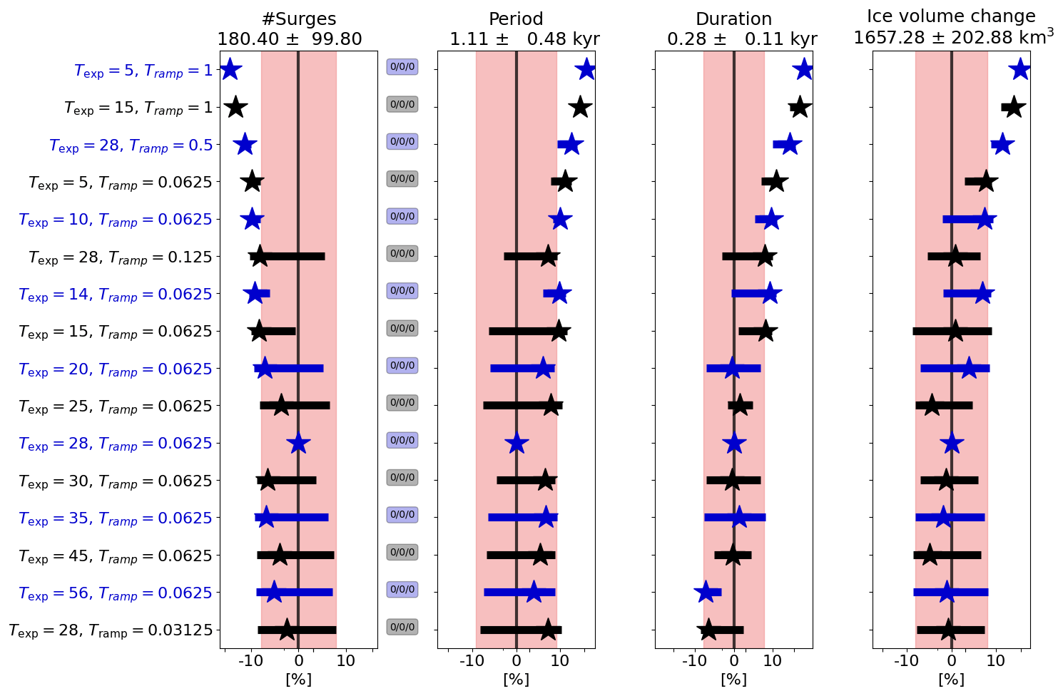
Figure 9 Percentage differences in surge characteristics compared to the GSM reference setup (T_ramp=0.0625, T_exp=28) for different basal-temperature ramps at 3.125 km horizontal grid resolution (average of the five parameter vectors). The ramps are sorted from widest (first row) to sharpest (last row; see Fig. S25 for a visualization of all ramps). Otherwise the same as Fig. 6. No runs crashed, and all runs had more than one surge. The exact values are given in Table S10.

Except for the three widest ramps, the mean ice volume bias is less than 1 %. The RMSE, on the other hand, is roughly 8 %, indicating that the average pseudo-Hudson Strait ice volume is similar, but the timing of surges varies even for small differences in the width of the ramp (Table S10).

We compare the different temperature ramps at 25, 12.5, and 6.25 km horizontal grid resolution by calculating a single score for the mean and standard deviation of all surge characteristics (Sect. S7.3). The ramps yielding the smallest differences compared to the 3.125 km reference setup are listed in Table S11 and shown in Fig. S26. These results may be different for a different reference setup (see Table S22 for a comparison of different reference setups with local basal hydrology).

At 25 km horizontal grid resolution, only 3 out of 12 basal-temperature ramps remain after removing the ramps for which the sum of scores (score mean + score SD, last column in Table S11) differs by more than 50 % from the minimum sum of scores (bold number in last column in Table S11). The minimum scores for the mean and standard deviation occur for the same ramp (T_exp=5, T_ramp=0.5), clearly identifying it as the ramp that best resembles the 3.125 km horizontal grid resolution reference runs. For the two finer horizontal grid resolutions, the minimum mean and standard deviation scores arise for different temperature ramps, preventing the determination of a single best ramp.

A more physically-based approach to determining an appropriate scale-compensating temperature ramp stems from our motivation for research question Q₅ above. We bundle all 3.125×3.125 km grid cells of our reference runs into patches of, e.g., 64 grid cells. Each patch represents a coarser (e.g., 25×25 km) grid cell. We then determine the warm-based fraction (basal temperature at the pressure-melting point) and the mean basal temperature with respect to the pressure-melting point of each patch. We can then estimate the parameters T_ramp and T_exp of the basal-temperature ramp (Eq. 8) by plotting the warm-based fraction against the mean basal temperature for all patches (e.g., Fig. 10) and fitting a basal-temperature ramp with the preliminary assumption that a corresponding coarse grid cell should have an ice-streaming fraction proportional to the sub-grid warm-based area.

However, this upscaling analysis does not account for the connectivity between the faces of, e.g., a 25 km grid cell. Without a continuous warm-based channel from one grid cell interface to another, there should be effectively no basal sliding across the grid cell, even when the average basal temperature is close to the pressure-melting point. Consequently, the best estimate for the two parameters of the basal-temperature ramp should be a lower bound to the points in the scatter plot.

Furthermore, the upscaling results depend on the bed properties (soft sediment vs. hard bedrock) and the specific scenario (surge vs. quiescent phase). Therefore, we only consider patches within the pseudo-Hudson Strait area during surges. Due to the limited storage capacity for the 10-year output fields, only the first 10 kyr after the first surge are used for the upscaling experiments.

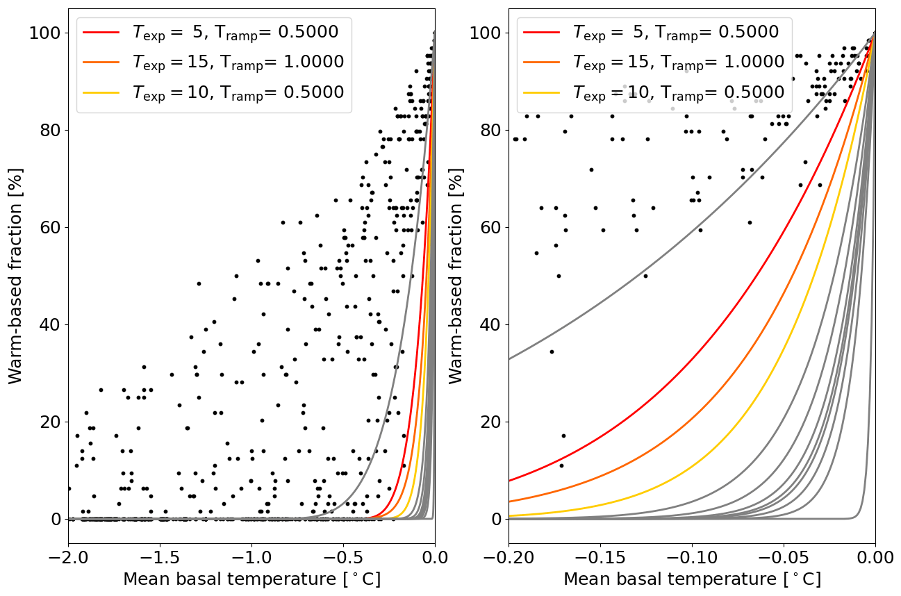
Figure 10 Warm-based fraction (basal temperature with respect to the pressure-melting point at 0 ^∘C) vs. mean basal temperature with respect to the pressure-melting point when upscaling a 3.125 km run to 25 km horizontal grid resolution including all five parameter vectors using the GSM. For example, an upscaled 25 km patch (containing 64 3.125 km grid cells) with 32 3.125 km grid cells at the pressure-melting point and 32 3.125 km grid cells at −1 ^∘C with respect to the pressure-melting point has a warm-based fraction of 50 % and a mean basal temperature of −0.5 ^∘C. Only grid cells within the pseudo-Hudson Strait and time steps within the surges of the 10 kyr after the first surge are considered. The restriction to the 10 kyr after the first surge for these experiments is set by storage limitations due to the high temporal resolution of the model output fields (10 years). The colored ramps correspond to the 25 km horizontal grid resolution basal-temperature ramps in Table S11, and the gray lines show all other ramps that were tested at this resolution.

The upscaling results agree well with the score analysis at 25 km horizontal grid resolution. Both indicate that, at this resolution, the ramp T_exp=5, T_ramp=0.5 (first row in Table S11, Fig. 10) gives results that best match those of the 3.125 km reference runs. The two approaches yield a similar range of temperature ramps at 12.5 and 6.25 km horizontal grid resolution, but the upscaling experiments generally favor wider temperature ramps (Table S11 and Figs. S27 and S28). This is likely a consequence of the above-mentioned role of sub-grid warm-based connectivity not accounted for in the upscaling analysis. When using the resolution-dependent ramp of Eq. (9), the upscaling experiments provide a lower bound of T_exp=5. Upscaling experiments with local basal hydrology lead to similar results.

3.3.4 Smooth sediment transition zone and non-flat topography

The effects of a smooth sediment transition zone (instead of an abrupt transition from hard bedrock (0 % sediment cover) to 100 % (soft) sediment cover) and a non-flat topography on surge characteristics are examined here.

The abrupt transition from hard bedrock to soft sediment (pseudo-Hudson Bay and Hudson Strait) in the GSM reference setup and the corresponding difference in basal-sliding coefficient provide an additional heating source due to shearing between slow- and fast-moving ice. This additional heat appears to foster the propagation of small surges along the transition zone (e.g., 6 to 6.3 kyr in the upper row of video 03 of Hank, 2023). Incorporating a smooth transition zone (3.125 km or 25 km wide) affects the location of the small-scale surges (not considered in surge characteristics) but shows only minor differences for the major surges (<7.5 % for all surge characteristics, Fig. 6). The mean bias for both widths is <1 %, indicating only minor differences in ice volume between an abrupt and smooth transition. However, the timing of surges varies for different transition zones (RMSE ≤8 %, Fig. 11). A wider transition zone (more sediment surrounding the pseudo-Hudson Strait and Hudson Bay) generally favors an earlier sliding onset (e.g., Fig. 11), but the details depend on the parameter vector in question.

Similarly to the GSM results, the PISM percentage differences between a smooth (reference setup) and abrupt sediment transition show no significant effect except for a 22 % increase in surge duration (Fig. 7).

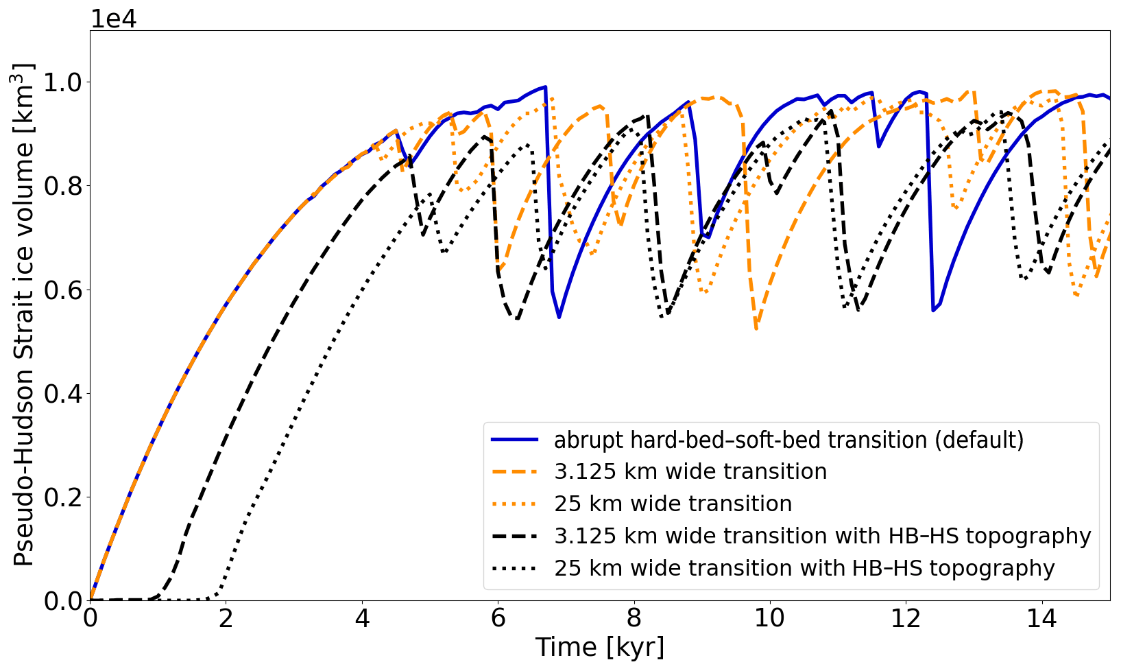
Figure 11 Pseudo-Hudson Strait ice volume for GSM parameter vector 1 and three different bed configurations. The horizontal grid resolution is 3.125 km. Note that the width of the topographical transition zone matches the width of the soft-bed–hard-bed transition zone. In experiments with a pseudo-Hudson Bay and Hudson Strait (HB–HS) topography, the pseudo-Hudson Strait topography is below sea level, increasing the time required for glaciation. A wider transition zone (larger area below sea level) leads to a later glaciation.

Adding a 200 m deep pseudo-Hudson Strait and Hudson Bay with a smooth transition zone and 500 m deep ocean to the GSM setup displaces the origin of surges slightly further inland. Due to both the resultant warmer basal temperature and depressed pressure-melting point, the surges propagate faster, last longer, and evacuate more ice volume (Fig. 6). The topography slopes down towards the pseudo-Hudson Strait, increasing the ice inflow from the surroundings. The ice sheet recovers faster from the previous surge, decreasing the mean period. Note that Fig. 6 shows an increase in the mean period, but this is somewhat misleading due to the now early surges for parameter vector 0 and the subsequent large increase in the mean period (∼100 % – no surges in the middle part of the run due to cold surface temperatures, Fig. S29). All other parameter vectors show a decrease in the mean period for both widths of the transition zone. The mean bias indicates a decrease in ice volume of ∼6.5 % for runs with a non-flat topography caused by the larger surges. The pseudo-Hudson Strait topography also suppresses the small surges otherwise observed in the vicinity of the pseudo-Hudson Strait. A detailed comparison of an individual run is presented in Sect. S7.4.

Comparing the results for two different widths of the topographic transition zone (−200 m to sea level) indicates fewer but stronger surges (increase of mean pseudo-Hudson Strait ice volume change by 9 %, Fig. 6) for a wider transition zone. The gentler slope increases the width of the ice stream and, thereby, the ice flux out of the pseudo-Hudson Strait (video 04 of Hank, 2023). The increased flux leads to a decreased pseudo-Hudson Strait ice volume at the end of the surge. The stronger surges for a wider transition zone increase the recovery time, leading to a smaller increase in the number of surges than for the narrow transition zone (difference of 16 %, Fig. 6).

While imposing a non-flat topography fosters surges in both models, the increase in mean ice volume change is much larger in PISM (390 %) than in the GSM (maximum ∼17 %), leading to a longer regrowth phase (79 % increase in mean period) and overall less ice volume (mean bias −30 %, Table S13). The longer recovery times in PISM outweigh the effect of earlier sliding onsets, which lead to more surges in the GSM (see above). Therefore, the number of surges decreases in PISM (while increasing in the GSM) when using a non-flat topography (Fig. 7).

Since the topography will vary from ice stream to ice stream, we stick to a flat topography for the remaining experiments.

3.3.5 Basal hydrology

The effects of adding a simple local basal-hydrology model to the GSM are examined here. The local basal hydrology sets the basal water thickness by calculating the difference between the basal-melt rate and a constant basal-drainage rate (rBedDrainRate in Table 1). This sub-glacial hydrology provides a simple and computationally efficient way to capture changes in basal-sliding velocities due to effective-pressure variations (Drew and Tarasov, 2022). However, it does not account for basal-ice accumulation, englacial or supraglacial water input, or horizontal water transport.

The basal water thickness (h_wb) and an estimated effective bed roughness scale (h_wb,Crit in Table 1) determine the effective-pressure coefficient:

$$\begin{array}{}\text{(19)}& N_{\mathrm{C},\mathrm{eff}}=\mathrm{1}-\min {\left({\displaystyle \frac{h_{\mathrm{wb}}}{h_{\mathrm{wb},\mathrm{Crit}}}},\mathrm{1.0}\right)}^{\mathrm{3.5}}.\end{array}$$

The basal water thickness is limited to $h_{\mathrm{wb},\mathrm{Crit}}=\mathrm{10}$ m and is set to h_wb=0 m where the ice thickness is less than 10 m and where the temperature with respect to the pressure-melting point is below −0.1 ^∘C. Experiments with $h_{\mathrm{wb},\mathrm{Crit}}=\mathrm{5}$ m yield the same results, and removing all the water for H<1 m, H<50 m, and $T_{\mathrm{bp}}<-\mathrm{0.5}$ ^∘C does not significantly (according to the MNEEs, Table 5) affect the model results. The effective pressure at the grid cell interface is then

$$\begin{array}{}\text{(20)}& N_{\mathrm{eff}}=g{\mathit{\rho }}_{\mathrm{ice}}\cdot \mathrm{0.5}\left(H_{\mathrm{L}}{N}_{\mathrm{C},\mathrm{eff},\mathrm{L}}+H_{\mathrm{R}}{N}_{\mathrm{C},\mathrm{eff},\mathrm{R}}\right),\end{array}$$

where g=9.81 m s⁻² is the acceleration due to gravity; ρ_ice=910 kg m⁻³ is the ice density; H is the ice thickness; and the subscripts L and R denote the adjacent grid cells to the left and right of the interface, respectively (this is similarly the case for upper and lower grid cells adjacent to a horizontally aligned interface). We enforce that N_eff never falls below $N_{\mathrm{eff},\min }=\mathrm{10}$ kPa (denominator in Eq. 21; similar results are found for $N_{\mathrm{eff},\min }=\mathrm{5}$ kPa). Finally, the effective pressure of each grid cell alters the basal-sliding coefficient in the sliding law (Eq. 6a) according to

$$\begin{array}{}\text{(21)}& C_{\mathrm{b}}=C_{\mathrm{b}}\cdot \min \left(\mathrm{10},\max \left(\mathrm{0.5},{\displaystyle \frac{N_{\mathrm{eff},\mathrm{Fact}}}{N_{\mathrm{eff}}+N_{\mathrm{eff},\min }}}\right)\right),\end{array}$$

where N_eff,Fact is the effective-pressure factor (Table 1). The change of the basal-sliding coefficient C_b is, therefore, limited to C_b⋅0.2 to C_b⋅10. Allowing a larger change of C_b⋅0.1 to C_b⋅20 does not significantly change the model results.

When running the GSM with the local sub-glacial hydrology model, intermediate values are used for all three parameters (the effective bed roughness scale $h_{\mathrm{wb},\mathrm{Crit}}=\mathrm{0.1}$ m, Eq. 19; the constant bed drainage rate rBedDrainRate ≃0.003 m yr⁻¹; and the effective-pressure factor $N_{\mathrm{eff},\mathrm{Fact}}\simeq \mathrm{63}\mathrm{246}$ Pa, Eq. 21) for all five parameter vectors. However, different values were tested for all three parameters (not shown). In general, a larger N_eff,Fact increases the basal-sliding coefficient (Eq. 21) and, therefore, leads to fewer but stronger surges. The results for h_wb,Crit and rBedDrainRate are not as straightforward to interpret. The model response varies for the two tested parameter vectors, and the changes are generally smaller than the MNEEs.

Adding the local basal hydrology model to the GSM increases the mean ice volume change and duration by 20 % and 12 %, respectively (Fig. 6, exceeding the MNEEs). The stronger surges are due to the reduction of effective pressure and, thus, increased sliding (Eqs. 21 and 6a). The mean period increases (17 %), while the number of surges decreases (−4 %), but the standard deviations are large.

Since the local hydrology model effectively increases the basal-sliding coefficient, we test if this impact can be replicated simply by increasing the sliding coefficients (Table 1) in a GSM configuration without basal hydrology. Doubling the soft-bed-sliding coefficient leads to similar or larger maximum basal-sliding velocities and, consequently, maximum ice fluxes but a smaller increase in the mean period (12 % vs. 17 %) and mean pseudo-Hudson Strait ice volume change (11 % vs. 20 %) than that of the local hydrology model. Increasing the hard-bed-sliding coefficient has no significant effect on the surge characteristics (pseudo-Hudson Bay and Hudson Strait are soft-bedded – Fig. 6). Intermediate increases in the basal-sliding coefficients (not shown) also do not capture the surge characteristics of the basal-hydrology model. Therefore, simply changing the basal-sliding coefficients cannot replace the basal-hydrology model.

3.3.6 Sensitivity experiments without a significant effect

The effect of an experiment is considered to be insignificant when the change in surge characteristics is smaller than the MNEEs (Sect. 3.2). This is the case for different weights of the adjacent minimum basal temperature when calculating the basal interface temperature (Q₆) for different implementations of the basal hydrology (Q₉) and when using basal hydrology instead of the basal-temperature ramp as the primary smoothing mechanism (Q₁₀). The details of these experiments are presented in Sect. S8.1, S8.2, and S8.3, respectively. We want to emphasize that experiments without a significant effect can still have physical relevance, but it is currently hidden within the numerical sensitivities.

3.4 Convergence study

In this section, we examine the horizontal grid resolution dependence of the GSM and PISM model results. Model results are considered to be converging when the differences in surge characteristics decrease with increasing horizontal grid resolutions.

3.4.1 GSM convergence study

Significant differences in surge characteristics occur when changing the horizontal grid resolution. These differences can be as large as a highly oscillatory behavior at 3.125 km and no oscillations at 25 km horizontal grid resolution (Fig. S23). Changing the basal-temperature ramp can somewhat counteract this discrepancy by enabling basal sliding at lower basal temperatures for coarser grid resolutions (Fig. S24 and video 05 of Hank, 2023). Further details on discrepancies between horizontal grid resolutions for individual parameter vectors are discussed in Sect. S9.1.

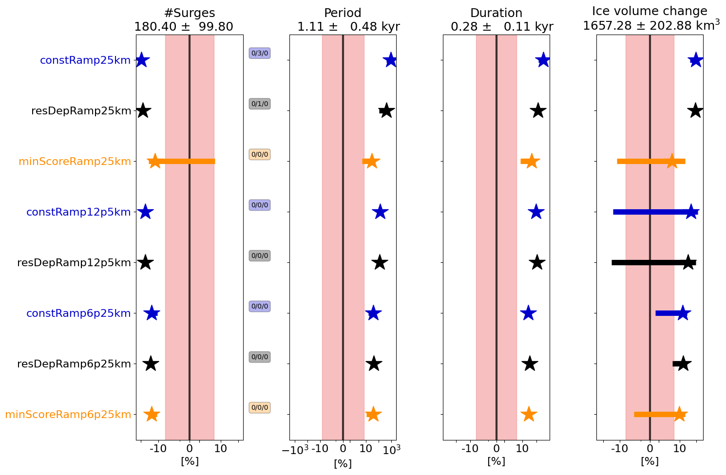
Figure 12 Percentage differences in surge characteristics compared to the GSM reference setup (3.125 km horizontal grid resolution) for model setups with coarser (25, 12.5, and 6.25 km) horizontal grid resolutions (average of the five parameter vectors). The different colors were added for visual alignment of the individual model setups and mark model setups with constant (blue), resolution-dependent (black), and minimum-score (orange, Sect. S7.3) basal-temperature ramps. The resolution-dependent ramps (T_exp=28) and constant ramps (black line, T_ramp=0.0625, T_exp=28) are shown in Fig. 2. The minimum-score basal-temperature ramps are T_ramp=0.5, T_exp=5 at 25 km and T_ramp=0.125, T_exp=45 at 6.25 km horizontal grid resolution. At 12.5 km, the minimum-score ramp is the same as the resolution-dependent ramp. Otherwise the same as Fig. 6. Further details of each individual experiment are provided in Sect. 3.4.1 and the Supplement.

We compare the differences in surge characteristics for different basal-temperature ramps at each resolution (Fig. 12). We examine a constant ramp (T_ramp=0.0625, T_exp=28), a resolution-dependent temperature ramp (T_exp=28, Fig. 2), and the ramp with the smallest differences in surge characteristics (bold mean score in Table S11). Note that the large differences in mean period at 25 km resolution are caused by long time intervals without any oscillations in the coarse-resolution runs (Table S18). The 25, 12.5, and 6.25 km runs show progressively smaller differences for the constant and resolution-dependent ramp, indicating model convergence. Convergence of the GSM results with increasing grid resolutions is further supported by successively smaller pseudo-Hudson Strait ice volume RMSE and mean bias values (Table S19). RMSE and mean bias are smaller across all resolutions when using a resolution-dependent ramp instead of a constant temperature ramp (except for the RMSE at 12.5 km horizontal grid resolution).

All three basal-temperature ramps lead to similar differences in surge characteristics at 6.25 and 12.5 km horizontal grid resolution (Fig. 12). At 25 km resolution, the ramp with the minimum differences in surge characteristics significantly improves the agreement with the 3.125 km runs, with differences that are smaller than for any other ramp or resolution. This could be a coincidence, or it could indicate that, despite thorough testing, the best ramp has not been found at 6.25 and 12.5 km horizontal grid resolution. Since other ramps at 25 km horizontal grid resolution show only slightly larger differences in surge characteristics (e.g., difference of 0.23 in the mean score, Table S11), it is unlikely that it is just a coincidence. However, the sensitivity of the surge characteristics to grid refinement remains, no matter the choice of the temperature ramp, with differences significantly exceeding the MNEEs from Sect. 3.2. Since including a sub-glacial hydrology model significantly affects the surge characteristics, we also examine the horizontal grid resolution scaling with a local-basal hydrology model (Sect. S9.2). The results show overall smaller differences (relative to the 3.125 km reference simulations) in surge characteristics than without a sub-glacial hydrology model (Table S22 vs. Table S18). The analysis of the convergence study (with and without basal hydrology) and the upscaling experiments in Sect. 3.3.3, therefore, suggest a resolution-dependent temperature ramp with T_exp between 5 and 10.

3.4.2 PISM convergence study

Similarly to the results presented for the GSM, the ice volume RMSE and mean bias show convergence under systematic grid refinement (Table S26). However, for the three resolutions examined here, the PISM surge characteristics show convergence for the mean duration and ice volume change but not the number of surges and mean period (Table S25). Note that four out of nine runs at 12.5 km horizontal grid resolution did not finish within the time limit of the computational cluster and are considered to be crashed runs (potentially skewing the statistics). Additionally, one run at 12.5 km resolution did not show any surges and was also excluded from the analysis. The differences in surge characteristics for different grid resolutions are, in general, larger than the MNEEs but can be smaller (mean ice volume change of the 25 km runs).

4 Results summary and discussion

This section summarizes our modeling results in the context of the research questions outlined in Sect. 1.3 and previous modeling studies.

4.1 Minimum numerical error estimates

Q₁

What is the threshold of MNEEs in the two models?

The MNEEs can be as large as 16 % (Tables 5 and 6). Given the non-linearities in the SSA (or higher-approximation) ice sheet system, there is no a priori reason to confidently assume other ice sheet models will have ignorable MNEEs for unstable contexts such as surge cycling and grounding-line response. Therefore, it is crucial to determine MNEEs (or a comparable threshold) to minimize the possibility of interpreting numerical errors as a physical response to a change in model setup.

In contrast to the findings of Souček and Martinec (2011), adding low levels of surface temperature noise does not significantly affect the GSM and PISM results (Tables S3 and S6). Potential reasons for the different model responses are the use of an Arakawa A grid (velocities and temperatures are calculated on the same node – Arakawa and Lamb, 1977) and the JOSH (JOint Shallow-ice/Higher-order model) ice sheet dynamics in Souček and Martinec (2011).

4.2 Sensitivity experiments with a significant effect

Q₂

Is the inclusion of a bed thermal model a controlling factor for surge activity?

Including a 1 km deep bed thermal model significantly (according to the MNEEs) affects the surge characteristics in the GSM and PISM. The additional heat stored in the bed changes the thermal conditions at the ice–bed boundary, dampening the ice volume change during a surge (Figs. 6 and 7). Models with similar setups but without a bed thermal model likely overestimate the ice volume change during a surge (e.g., Calov et al., 2010; Brinkerhoff and Johnson, 2015). Therefore, the inclusion of a bed thermal model is a key aspect of modeling ice stream surge cycling.

Q₃

Do different approaches for determining the grid cell interface basal temperature significantly affect surge behavior, and if yes, which one should be implemented?

The choice of approach for determining the basal temperature at the grid cell interface significantly changes the surge characteristics. Without considering additional heat transfer to the grid cell interface (as an attempt to represent heat contributions from sub-glacial hydrology and sub-grid ice advection), the number of surges decreases by at least 75 %. The additional heat is, therefore, an essential component for modeling surges in the GSM.

This additional heat transfer to the grid cell interface is comparable to spreading 50 % of the basal-heating effect from sliding in a grid cell to the surrounding grid cells used in mPISM (latest version based on PISM v0.7.3, e.g., Ziemen et al., 2014, 2019; Schannwell et al., 2023). This spreading of basal heating warms the grid cells adjacent to an ice stream and was necessary to model Heinrich-event-like surges (Florian Ziemen, personal communication, 19 May 2022). While no additional heat transfer was added to PISM v2.0.2 used within this study, the till friction angles had to be reduced to model surges.

Q₄

How different are the model results for different basal-temperature ramps? And what ramp should be used?

Similarly to Souček and Martinec (2011), we find significant differences in the period and amplitude of surges at all tested resolutions when using different implementations for thermal activation of basal sliding (the basal-temperature ramp). In the GSM, a wider temperature ramp enables sliding onset at lower temperatures, fostering more extensive surge propagation and leading to stronger surges. However, the choice of the most appropriate temperature ramp at the finest resolution tested (3.125 km, Fig. 9) is unclear, and identifying a single best ramp (fit of coarse-resolution runs to 3.125 km runs) is challenging (Table S11). In general, a resolution-dependent ramp with T_exp between 5 and 10 (Eqs. 8 and 9) yields the smallest differences between fine- and low-resolution simulations. However, given potential dependencies on the particular ice sheet model, we recommend resolution testing to determine the optimal basal-temperature ramp. Nevertheless, a basal-temperature ramp (or similar mechanism) should be implemented in all ice sheet models for contexts where surge onset and/or termination are important.

Q₅

Does the abrupt transition between a soft and hard bed significantly affect surge characteristics?

Incorporating a smooth transition zone with two different widths (3.125 and 25 km) in the GSM does affect the location of proximal small-scale ice streams (video 03 of Hank, 2023). However, the abrupt transition is not the cause of the major surges in the GSM (Fig. 6) and PISM experiments (Fig. 7). Since the sediment cover can change within a few kilometers (e.g., Andrews and MacLean, 2003), we conclude that, despite the minor differences, an abrupt transition between soft and hard beds is a reasonable simplification, especially considering horizontal grid cell dimensions of 25 km or larger.

Q₆

How does a non-flat topography affect the surge behavior?

Imposing a non-flat topography leads to significantly longer and stronger surges (Figs. 6 and 7). As such, and in agreement with previous modeling studies (e.g., Winsborrow et al., 2010, and references within), ice streaming is sensitive to the basal topography.

Q₇

What is the effect of a simplified basal hydrology on surge characteristics?

Activating the local basal-hydrology model (including the addition of effective-pressure dependence into the sliding law) in the GSM significantly increases the surge duration and amplitude (Fig. 6). Somewhat stronger surges are expected due to the reduction in effective pressure introduced by the sub-glacial water. Model runs without sub-glacial hydrology will therefore tend to underestimate the strength of surges. In general, this also holds for subglacial hydrology models with higher complexity (Drew and Tarasov, 2022). The importance of sub-glacial hydrology has also been shown in several other studies examining the effects of ice sheet surges and ice streaming within a continuum model approach (e.g., Fowler and Johnson, 1995; Fowler and Schiavi, 1998; Benn et al., 2019).

4.3 Sensitivity experiments without a significant effect

Q₈

How much of the ice flow should be blocked by upstream or downstream cold-based ice, or equivalently, what weight should be given to the adjacent minimum basal temperature?

Changing the weight of the adjacent minimum basal temperature for the basal-sliding temperature ramp in the GSM yields a maximum difference of 15 % (Table S15). These somewhat small effects on surge characteristics are likely due to the fact that most surges propagate upstream (from the ocean to the pseudo-Hudson Bay), and the adjacent minimum basal temperatures (almost exclusively located upstream) have little potential to affect (e.g., partly block) the ice flow.

Q₉

How significant are the details of the basal-hydrology model to surge characteristics in PISM?

Incorporating a mass-conserving horizontal-transport hydrology model does not significantly change the surge characteristics in PISM (Fig. 7), indicating that the computationally much cheaper local hydrology model is a reasonable simplification for this context. More nuanced results, depending on the surge characteristics examined, are observed for the GSM (Drew and Tarasov, 2022).

Q₁₀

What are the differences (if any) in surge characteristics between local basal hydrology and a basal-temperature ramp as the primary smoothing mechanism at the warm-based–cold-based transition zone?

Once included, the local basal hydrology is the primary smoothing mechanism. However, since the two smoothing mechanisms operate in different temperature regimes, a basal-temperature ramp (representing sub-temperate sliding) cannot be replaced by a basal-hydrology scheme (as in, e.g., Robel et al., 2013; Kyrke-Smith et al., 2014; Brinkerhoff and Johnson, 2015). The differences in surge characteristics are smaller than the MNEEs, preventing further analysis.

4.4 Convergence study

Q₁₁

Do model results converge (decreasing differences when increasing horizontal grid resolution)?

In general, both models exhibit convergence under systematic horizontal grid refinement for the overall ice volume (mean bias, Tables S19, S23, and S24), but the solution is not fully converged at the finest resolutions tested. However, while all surge characteristics converge for the GSM (Table S18), PISM results do not show convergence for the number of surges and mean period (Table S25). This clearly illustrates that mean ice volume and, consequently, mean ice thickness, as presented, e.g., in Van Pelt and Oerlemans (2012), are insufficient metrics to determine whether cyclic model results exhibit a resolution dependency.

While other studies examining thermally induced ice streaming do not find a strong resolution dependence (Hindmarsh, 2009; Brinkerhoff and Johnson, 2015), these studies are not directly comparable. The different results are likely due to differences in the experimental design. For example, neither Hindmarsh (2009) nor Brinkerhoff and Johnson (2015) consider a bed thermal model. While Hindmarsh (2009) considers sub-temperate sliding, his model allows sliding far below the pressure-melting point (order of δ=1 compared to δ=0.01 within this study – Eq. 10) and focuses on steady ice streaming and not ice stream surge cycling. Both of the above studies analyze just one parameter vector, and there are some parameter vectors for which, e.g., the GSM exhibits only a minor resolution dependence.

Even though the studies are not directly comparable, the results of Brinkerhoff and Johnson (2015) offer some insight relevant to this study. For example, they suggest that membrane stresses are necessary for convergence under horizontal grid refinement. The hybrid SIA–SSA ice dynamics used in the GSM and PISM might be insufficiently higher order and lead to a stronger resolution dependence than the schemes used in Hindmarsh (2009) and Brinkerhoff and Johnson (2015). However, GSM experiments with the SSA active everywhere show a resolution dependence comparable to the velocity-dependent SSA activation criteria (Table S24 and S18, respectively), indicating that the hybrid SIA–SSA ice dynamics are not the sole reason for the strong resolution dependence.

5 Conclusions

Within the limitations of hybrid SIA–SSA ice dynamics, we investigate the effect of ice sheet model numerics and discretization choices on surge characteristics often neglected in ice sheet modeling studies. We show how to reduce numerical and discretization sensitivities given finite computational resources and then how to determine the significance of model results given residual computationally unavoidable numerical sensitivities for surge cycling contexts. In particular, our analyses offer guidance on minimizing the resolution dependency by implementing a resolution-dependent basal-temperature ramp for basal-sliding thermal activation and increasing confidence in model results by determining minimum numerical error estimates (MNEEs). Based on these MNEEs, our results indicate that surge characteristics are significantly affected by the inclusion of a basal-hydrology model. Not including the dampening effect of a bed thermal model on basal-temperature changes, as has been the tendency in idealized process studies, overestimates the surge amplitude. The key takeaways of this study are the physical modeling choices and numerical sensitivities that must be considered when numerically modeling ice stream surge oscillations.