the Creative Commons Attribution 4.0 License.
the Creative Commons Attribution 4.0 License.
 | 06 Oct 2023
Emulating lateral gravity wave propagation in a global chemistry–climate model (EMAC v2.55.2) through horizontal flux redistribution
Sebastian Rhode
Hella Garny
Peter Preusse
Petr Pisoft
Aleš Kuchař
Patrick Jöckel
Astrid Kerkweg
Bastian Kern
The columnar approach of gravity wave (GW) parameterisations in weather and climate models has been identified as a potential reason for dynamical biases in middle-atmospheric dynamics. For example, GW momentum flux (GWMF) discrepancies between models and observations at 60∘ S arising through the lack of horizontal orographic GW propagation are suspected to cause deficiencies in representing the Antarctic polar vortex. However, due to the decomposition of the model domains onto different computing tasks for parallelisation, communication between horizontal grid boxes is computationally extremely expensive, making horizontal propagation of GWs unfeasible for global chemistry–climate simulations.
To overcome this issue, we present a simplified solution to approximate horizontal GW propagation through redistribution of the GWMF at one single altitude by means of tailor-made redistribution maps. To generate the global redistribution maps averaged for each grid box, we use a parameterisation describing orography as a set of mountain ridges with specified location, orientation and height combined with a ray-tracing model describing lateral propagation of so-generated mountain waves. In the global chemistry–climate model (CCM) EMAC (ECHAM MESSy Atmospheric Chemistry), these maps then allow us to redistribute the GW momentum flux horizontally at one level, obtaining an affordable overhead of computing resources. The results of our simulations show GWMF and drag patterns that are horizontally more spread out than with the purely columnar approach; GWs are now also present above the ocean and regions without mountains. In this paper, we provide a detailed description of how the redistribution maps are computed and how the GWMF redistribution is implemented in the CCM. Moreover, an analysis shows why 15 km is the ideal altitude for the redistribution. First results with the redistributed orographic GWMF provide clear evidence that the redistributed GW drag in the Southern Hemisphere has the potential to modify and improve Antarctic polar vortex dynamics, thereby paving the way for enhanced credibility of CCM simulations and projections of polar stratospheric ozone.
- Article
(6242 KB) - Full-text XML
- Companion paper
-
Supplement
(9841 KB) - BibTeX
- EndNote


The middle atmosphere is an important part of Earth's atmospheric system, housing the ozone layer and global-scale dynamic processes. This includes the Brewer–Dobson circulation (BDC, Brewer, 1949; Dobson, 1956), which controls the transport of radiatively active trace gases in the stratosphere and mesosphere. Moreover, middle atmosphere dynamics are a notable source of uncertainties for decadal to centennial climate projections as well as for medium-range weather forecasts due to dynamical downward coupling mechanisms (see e.g. Hardiman and Haynes, 2008; Gerber et al., 2012; Hitchcock and Simpson, 2014). In high latitudes, these coupling mechanisms are strongly connected to the strength and stability of the polar vortices. The momentum and energy that dissipate when upward-propagating atmospheric waves break are crucial for the polar vortices and for other dynamical phenomena such as the semi-annual oscillation (SAO; Baldwin and Dunkerton, 2001) and the quasi-biennial oscillation (QBO; Giorgetta et al., 2002) in the middle atmosphere (e.g. Charney and Drazin, 1961; Andrews et al., 1987; Šácha et al., 2019). These atmospheric waves are commonly induced in the troposphere and propagate upward, thereby transporting momentum and energy to the middle atmosphere. The global spectrum of atmospheric waves spans from small-scale gravity waves (GWs) with wavelengths of the order of ∼ 10–1000 km to large-scale planetary waves. The resolution of current climate models is fine enough to capture the planetary waves and their propagation and dissipation. GWs, on the other hand, occur on small spatial scales and short timescales, and at least parts of the GW spectrum cannot be resolved by current state-of-the-art climate models and therefore have to be parameterised. GW parameterisations in general circulation models (GCMs) are commonly subdivided into non-orographic GWs and orographic GWs (OGWs), referring to different GW sources. The latter explicitly concerns mountain waves (MWs) originating from flow over orography, while the former takes into account all other GW sources, e.g. convection, frontal instabilities or spontaneous adjustment (see e.g. Fritts and Alexander, 2003; Alexander et al., 2010). Both GW schemes were historically included in weather and climate models and tuned in order to eliminate or alleviate dynamical model biases (see e.g. Palmer et al., 1986; Giorgetta et al., 2002; Shepherd, 2007). OGWs, for example, helped to separate the stratospheric polar night jet from the tropospheric subtropical jet (Kim et al., 2003; Alexander et al., 2010; Eichinger et al., 2020). Today, various versions of these parameterisation schemes (e.g. Lott and Miller, 1997; Gregory et al., 1998; Scinocca and McFarlane, 2000) are still routinely applied in GCMs for climate simulations, but as the understanding of GW processes grows, parameter specifications are constantly further developed (e.g. de la Cámara et al., 2014; Garcia et al., 2017; Xie et al., 2020; Plougonven et al., 2020; van Niekerk and Vosper, 2021; Xie et al., 2021; Ribstein et al., 2022).
The main interactions of GWs with prognostic quantities in GCMs are deceleration and acceleration of the winds at the location of wave breaking as well as energy transfer in the form of temperature; these need to be parameterised as correctly as possible. GWs propagate not only upwards, but also horizontally, and this lateral GW propagation has multiple effects (Song et al., 2007; Fritts et al., 2016; Samtleben et al., 2019; Strube et al., 2021). First and foremost, it leads to a relocation of GWMF and therefore GW drag. An indirect consequence is that GWs propagate upwards in other locations and thereby may encounter critical levels at different altitudes. Since GW drag is a function of GWMF and inverse density, which decreases with altitude, it potentially also leads to a decrease or increase in total GW drag depending on the altitudes of GW breaking (e.g. Xu et al., 2017).
GW parameterisations in GCMs are implemented in a purely columnar manner, not allowing any horizontal propagation of GWs and their momentum. This is despite the fact that numerous studies have analysed lateral GW propagation (e.g. Preusse et al., 2002; Sato et al., 2012; Kalisch et al., 2014; Fritts et al., 2016; Perrett et al., 2021; Strube et al., 2021), and GWMF discrepancies between models and observations could largely be attributed to this process, particularly at 60∘ S (Geller et al., 2013; Kruse et al., 2022). Moreover, the spatio-temporal OGW distribution has been shown to be important for planetary-scale wave fields via modification of refraction conditions (Šácha et al., 2016, 2021; Samtleben et al., 2019, 2020), and the lack of horizontal propagation has been suggested to be a source of zonal wind biases in the Antarctic polar vortex (McLandress et al., 2012; Gupta et al., 2021). However, due to the decomposition of the model domains onto different computing tasks for parallelisation, communication between horizontal grid boxes can become computationally extremely expensive, making lateral propagation unfeasible in multi-decadal global climate simulations. For example, Song et al. (2007) implemented a spectral parameterisation of GW drag induced by cumulus convection in a three-dimensional framework in a chemistry–climate model (CCM). Likely due to the computational cost of the development, this could not be established for operational use in the model.
To overcome this issue, while retaining computational efficiency and flexibility, we present a solution that emulates lateral GW propagation through redistribution of the orographic GWMF in a CCM at a single altitude with tailor-made redistribution functions. These global redistribution functions describe a general propagation pattern of MWs and are generated by use of a mountain wave model (MWM), which was developed particularly for this purpose and is described in detail by Rhode et al. (2023). There, the authors showed the capability of the model to reproduce lateral propagation patterns found in satellite and high-resolution simulations. For example, strong leeward OGW propagation has been found, which is in agreement with Sato et al. (2012). Within this MWM, an orography is described as a set of idealised mountain ridges, with each exciting a specific MW. The idealised mountain shape allows estimation of the location, orientation, horizontal wavelength and displacement amplitude of launched MWs. The temporal and spatial propagation of these MWs is calculated using the ray tracer GROGRAT (Gravity-wave Regional Or Global Ray Tracer; Marks and Eckermann, 1995; Eckermann and Marks, 1997). In the global CCM EMAC (ECHAM MESSy Atmospheric Chemistry, v2.55.2; Jöckel et al., 2010, 2016), these maps then allow redistribution of the GWMF horizontally, obtaining an affordable overhead of computing resources, independent of the model decomposition in grid point space.
A schematic of our approach is shown in Fig. 1. First, the redistribution of GWMF is determined by means of a ray-tracing model. To do so, GWs are initialised from each source grid cell, and their locations (lat, long) are detected and weighted by their GWMF at a fixed altitude, the target height Htar. These locations are then taken as the target location of the GWMF transport. In EMAC, this redistribution map (μrd) is applied at a different height, the redistribution height Hrd, where the total column GWMF is redistributed to the predetermined target locations with the given weight. This approximates the horizontal momentum transport of the ray-traced GWs from lateral propagation. The redistribution height should be lower than the target height for a better approximation of the GW propagation pattern in the CCM.
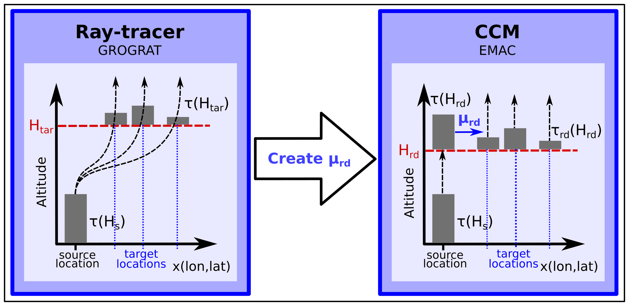
Figure 1Schematic of the redistribution approach with example momentum propagation paths. The momentum transport target locations are estimated at a fixed target height, Htar, and weighted by the GWMF of the respective GWs. This pattern of horizontal transport (the redistribution map μrd) is applied in EMAC at the redistribution height, Hrd, which should be lower than Htar. Energy conservation is preserved by only redistributing the GWMF that EMAC computes in the source column just below Hrd, i.e. by .
In Sect. 2, we describe the employed ridge parameterisation and the coupled ray tracer GROGRAT. Further, the generation of the redistribution maps with this model system is presented and exemplary redistribution patterns are shown. Moreover, analyses to determine the ideal ray target height for the generation of optimal redistribution functions and the ideal altitude at which the redistribution should be applied in the CCM are given. In Sect. 3, implementation of usage of the redistribution functions to horizontally redistribute orographic GWMF in the CCM EMAC is described, and the details in the used Lott and Miller (1997) orographic GW parameterisation scheme are presented. Moreover, a scaling analysis to evaluate the additionally required computing time and an update to the subgrid-scale orography to high-resolution elevation data is provided. The section proceeds with the results of test simulations with the new CCM implementations and with a brief analysis of their influence on Antarctic polar vortex dynamics. To wrap up the paper, a summary and several discussion points are presented in Sect. 4.
Here, redistribution maps that describe an approximated propagation pattern of OGWs are generated by means of a mountain wave model (MWM). This is done in three steps: (i) mountain ridge identification for MW source estimation, (ii) ray tracing for propagation of MWs through the atmosphere and (iii) evaluation of the results to generate redistribution maps. These three steps are described in detail in the following sections. The idea is that the redistribution maps are linear transformations of GWMF fractions from source grid cells to target grid cells. The values of the transformation are proportional to the amount of GWMF that has been transported from a source to the corresponding target grid cell. Additionally, in Sect. 2.4 an assessment of ideal values for free parameters in these transformations is presented.
2.1 The ridge parameterisation
First, we apply an algorithm to detect and parameterise mountain ridges from topographic data to retrieve MW parameters and to analyse the MW spectrum and distribution that needs to be initialised in the ray-tracing model. The approach applied here is described in detail in the companion paper, Rhode et al. (2023), and it is similar to the one performed by Bacmeister (1993) and Bacmeister et al. (1994). The topography data set used, “ETOPO1” (Amante and Eakins, 2009), features a 1 arcmin resolution.
The general idea is to represent the topography in terms of a small number of idealised Gaussian-shaped mountain ridges. For this, different bandpass filters between about 100 and 1500 km of varying widths are applied to the topography for scale separation. A skeleton of the bandpass-filtered topography is generated through a reduction to the ridge lines of the field, represented by the mountain crests. Locations where idealised ridges will be fitted are singled out using a Hough transformation. This results in approximately straight mountain ridge location candidates. At these, a fit with a Gaussian-shaped mountain ridge (Gaussian shape across the mountain, constant along the ridge) is performed in order to minimise the absolute difference of the idealised ridge to the bandpass-filtered topography. The Gaussian mountain shape has been used in many MW studies and allows straightforward conversion of ridge parameters, i.e. width and height, to the initial GW parameters, i.e. wavelength and amplitudes. Applying this algorithm to all spectral bands results in a ridge collection of Gaussian-shaped mountains that approximate the underlying topography in the chosen length scales.
Further, it is assumed that each of these mountains excites an MW with displacement amplitude δ proportional to the best-fit height h (for sufficiently strong winds ) and horizontal wavelength λhor=2πσ, where σ denotes the width of the Gaussian. A possible reduction in amplitude due to weak low-level winds, i.e. wind blocking, is accounted for as is a reduction in amplitude if the flow is perpendicular to the ridge (e.g. Barry, 2008). For initialisation, MWs are assumed to always launch perpendicular to the source ridge, which is in line with previous studies on MWs (e.g. Hines, 1988; Bacmeister, 1993) and can be seen in observations and model data as well (Kruse et al., 2022). For more details and validation of this approach, see Rhode et al. (2023).
2.2 The ray tracer GROGRAT
For the propagation of initialised MWs, the ray tracer GROGRAT (Gravity-wave Regional Or Global Ray Tracer; Marks and Eckermann, 1995; Eckermann and Marks, 1997) is used. GROGRAT is a global ray-tracing model describing the propagation, amplitude evolution and dissipation of atmospheric GWs within the limits of linear GW theory. It calculates four-dimensional GW ray trajectories in a non-hydrostatic atmosphere through use of non-linear differential equations derived from the dispersion relation based on WKB (Wentzel–Kramer–Brillouin; e.g. Bretherton, 1966) theory. Under consideration of meteorological background fields, GROGRAT integrates these differential equations numerically to calculate the GW trajectories. The (horizontal wind) amplitudes are calculated from the vertical flux of wave action density under the assumption that this is a conserved quantity along the ray path except for saturation and breaking. Wave breaking is assumed if the wave amplitude is large enough to break local dynamic stability, i.e. the wave reaches its saturation amplitude, which is described by Fritts and Rastogi (1985). In addition, waves are damped along their trajectory due to turbulence and radiation.
In the present study, the trajectory calculations for the MWs initialised from the ridge collection of Sect. 2.1 are performed using ERA5 reanalysis data (Hersbach et al., 2020) as background meteorological conditions. These data are provided on a 0.25∘ horizontal, 1 km vertical grid and with 6 h time resolution.
2.3 Redistribution maps
We apply the mountain wave model (MWM), i.e. the ridge parameterisation coupled to the ray tracer GROGRAT, as described in Sect. 2.1 and 2.2 to generate global horizontal redistribution maps for use in the CCM EMAC in the next step. The ray tracer provides all necessary information to quantify momentum transport due to propagating MWs, i.e. location, amount of GWMF, and horizontal as well as vertical wavelengths, and is therefore a suitable tool to generate the redistribution matrices approximating the GWMF transport.
The redistribution of GWMF corresponds to a mapping from source grid cells to target grid cells with the transformation values proportional to the amount of GWMF that has been transported from a source to the corresponding target grid cell. The grid cell size can be chosen based on individual needs and determines how many individual MWs, and therefore GWMF, are averaged over in the source as well as in the target grid cells. Hence, we generate a four-dimensional map μrd (ϕsrc, φsrc, ϕtar, φtar) describing the general MW propagation pattern. Here, ϕ and φ denote latitude and longitude, respectively; the subscript src refers to the source grid cell, i.e. the location at which the MW was excited; and tar refers to the target grid cell, i.e. the grid cell to which the MW's GWMF is transported. The map entries are generated by adding up the GWMF in the corresponding target location at a given altitude Htar from all source cells for each MW. Since the ray tracer provides only the peak value of GWMF and we need to account for the total GWMF of the wave, we scale the contribution of each MW by its horizontal wavelength and the length of the source ridge exciting the particular wave. This considers the effect that waves with a wider horizontal extent have a more spread-out footprint in physical space than small localised ones of the same peak GWMF. The latter is the case if we assume that GW packets extend the same number of wavelengths at any scale, which is reasonable because we only consider GWs of a single origin (mountain waves). The resulting redistribution map is scaled such that
This normalisation ensures energy conservation in the sense that we only redistribute what the model already initialised. Thus, for each source grid cell, we end up with a probability map that defines to which target cells which fraction of the GWMF is transported. For consistency, this normalisation is also enforced for source cells where no MWs are initialised (e.g. above the ocean) by not assuming any horizontal transport, i.e. μrd=1 at the source grid cell and 0 in all other grid cells. The effect of the target height Htar, which is the height at which the position of the MW is taken as the transport target, on the redistribution maps and resulting redistribution maps is investigated in Sect. 2.4.
To generate the redistribution maps, global fields of the zonal and meridional wind components, temperature, and pressure are required as meteorological background conditions. For this, data from models or reanalyses can be taken; here we chose the ERA5 reanalysis (Hersbach et al., 2020). As an example of the redistribution (or probability) maps, Fig. 2a shows the target values of the redistribution for MWs initialised at 48.8∘ S, 70.3∘ W. This example redistribution map was produced from 1 month of ERA5 data for July 2006 with a target altitude of 40 km. The redistribution map shows that only little of the GWMF that originates from the source grid cell will stay in this box, and therefore in the model column, after redistribution. Most of it will be redistributed to grid cells downwind, a large part to the southeast towards the Drake Passage. Therefore, the CCM should show increased drag at 60∘ S after redistribution. The rather large spread of GWMF transport can be attributed to a variety of different wind situations. But also the relatively large grid size used here (∼ 2.8∘ × 2.8∘) leads to the inclusion of many differently oriented ridges in one cell within the MWM consideration. This grid size was chosen as it represents the standard EMAC horizontal resolution setup of T42. Moreover, Fig. 2b shows the same redistribution map summed over all source grid cells to display the total redistribution from all grid boxes. It is an indicator of where to expect enhanced and reduced GWMF (considering only relative inflow and outflow). As expected, we see a reduction above land as well as an enhancement above the ocean, and the transport is mainly in the direction of the predominantly eastward winds. But in the northern parts of the shown section, there is also a small region above land with values larger than 100 %. As the percentage values of the cumulative redistribution fractions of all source grid cells are depicted in Fig. 2b, this does not necessarily mean an increase in GWMF after redistribution.
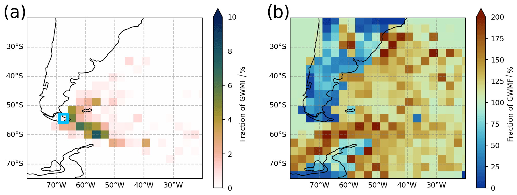
Figure 2(a) Exemplary redistribution function for the source grid box at 48.8∘ S, 70.3∘ W (light blue square). Colour shading shows the target cell percentage of the GWMF transported from this source grid. (b) Redistribution map summed over all source grid boxes to provide an estimate of the total GWMF redistribution if all source grid cells exerted the same amount of GWMF. The colour shading corresponds to the percentage of GWMF ending up in the respective grid cell; blue cells result in reduced and red cells in increased GWMF values.
2.4 Assessment of redistribution maps and ideal height parameters
As indicated above and illustrated in Fig. 1, the implementation of the GW redistribution in EMAC depends on the two parameters target height, Htar, and redistribution height, Hrd. The target height defines the altitude at which the horizontal location of the GWs is taken as the target location for generating the redistribution maps with the MWM. In general, the higher this altitude is, the further the GWs will have propagated from their source and the more spread out the redistribution map will be. This can be used to tune the redistribution map with respect to the locations and altitudes of GW activity. The redistribution height defines the level at which the redistribution of GWMF is performed in EMAC. In other words, it is the altitude above which GWMF in EMAC is no longer restricted to the source location, but instead once distributed to the locations determined by the redistribution map. And again, these locations are estimated from the MWM at the target height.
To find the ideal estimates for these parameters, we approximate the effect of GW redistribution on GWMF distributions using the MWM. For this, we firstly apply the MWM in a columnar manner by restricting the GWs to their source location, i.e. without lateral propagation, in the following called “NO_HOR”. Secondly, we apply the GW redistribution in the columnar-mode MWM in nine simulations for redistribution maps generated with varying Htar (10–50 km in 5 km steps), mimicking the implementation in EMAC that will be described later in Sect. 3. Thirdly, we use the MWM allowing full lateral propagation of GWs, i.e. in the same configuration that was also used to generate the redistribution maps. The latter will be considered our ground truth for this assessment, i.e. used as a reference and called REF in the following. Note that, for now, we are only considering a variable target height, Htar, to assess the ideal Htar for generating the redistribution maps. An optimised value for the redistribution height, Hrd, will be estimated later on in this section.
Figure 3a–b and d–e show vertical profiles of GWMF and GW drag deviations of the NO_HOR simulation and the simulations with GW redistribution with respect to the fully propagating REF simulation. The deviations are taken as the relative deviation from REF at each grid point location and averaged globally and over the month. Here the redistribution height is fixed to the lowermost level. This means that all simulations are different at all levels due to the different redistribution maps for each case.
First, we look at the results from the simulations with redistribution maps of July 2006 applied to the same month (Fig. 3a–c). Figure 3a shows improved agreement in GWMF (always with regard to REF) through GW redistribution. In the upper stratosphere, the mean deviation in GWMF drops from 140 % in the columnar case to about 60 % depending on the target height. Similarly for the drag in Fig. 3b, the deviation drops from about 160 % to 80 %–90 %. There is a trade-off evident here: the higher the target height, the better the agreement of the wave field in the upper atmosphere, but the more overestimated the propagation of MWs at lower altitudes. Since dissipating MWs primarily interact with the general circulation by exerting drag and thus changing the model winds, our main objective is to calculate the relocation of the (total) drag as correctly as possible.
As atmospheric density decreases with altitude, the relative deviations as shown in Fig. 3b will have a stronger effect in the upper atmosphere. Therefore, Fig. 3c shows the reduction in total deviation with respect to the columnar simulation, which is proportional to the area between the black and the coloured curves of Fig. 3a and b (scaled with the respective GWMF or drag at each altitude level). The reduction in deviation by redistribution is equivalent to a reduction in area between the GWMF or drag profile and zero. The best representation of GWMF transport is achieved with a target height of about 25 km. This rather low altitude is a consequence of GWMF of primary MWs diminishing with altitude in general. In contrast to this, the optimum for drag is reached at a target height of about 40 km. As most MWs dissipate their momentum in the upper stratosphere, we mainly focus on improving GW drag at these altitudes.
Next, we repeat the assessment with a redistribution map that was generated from propagation patterns averaged over the entire year of 2006 to yield a more general result. As before, the redistribution maps were applied to simulations of July 2006. The results of these simulations (Fig. 3d and e for GWMF and drag, respectively) are similar to the redistribution map generated from July data. After GW redistribution, the GWMF deviations are larger than with the columnar approach below around 15 km, but smaller above. The same applies to GW drag, where the deviation is particularly reduced around 10–20 km. This is where the summertime stratospheric wind reversal is located, hence possibly causing an impact on model dynamics through GW redistribution.
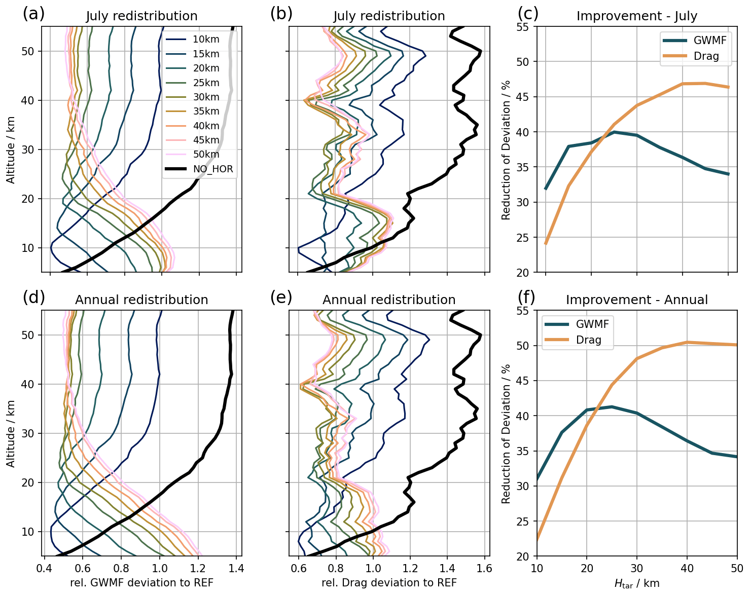
Figure 3Comparison of MWM simulations with GW redistribution (with varying Htar, coloured lines) and vertical-only propagating MWM simulations (NO_HOR, black lines) to a simulation including horizontal propagation (REF) for (a, d) GWMF and (b, e) GW drag. To show the effect of the target height, Htar, the GW redistribution is performed at the lowermost level in these four panels, leading to profile differences at all altitudes. The horizontal axis shows the relative deviation from REF at the corresponding altitude in the monthly and global mean. Panels (c) and (f) show the maximum improvement (reduction of deviation from REF) for different Htar with optimal redistribution height (i.e. the redistribution takes place at the cross-over of the black and the respective coloured curve). This is proportional to the area between the black and the coloured curves in panels (a) and (b) (only to the left of the black curve). The redistribution maps were generated from simulations of July 2006 in panels (a)–(c) and from simulations of the entire year of 2006 in panels (d)–(f) and applied to simulations of July 2006 in both cases.
For the cumulative improvement across all altitudes using the annual mean redistribution map, Fig. 3f shows the reduction in total deviation. The optimal target height is still 25 km considering GWMF and 40 km for GW drag, with the GW drag being of higher relevance for our purpose. Therefore, we determine the target height to be 40 km in all following simulations. Note that the total agreement in GWMF and GW drag transport is better with the annual redistribution map compared to the July-only redistribution map. This can be explained by improvements in the summer hemisphere as well as by an increase in statistics, as there are now 12 times as many ray traces considered.
The next question is where the ideal redistribution height is for a fixed Htar of 40 km. For this, we search for the minimum difference to the REF simulation through GW redistribution at different altitudes, i.e. the altitude where the coloured lines in Fig. 3b and e cross the black line. In principle, such an optimal redistribution height could be found for any specific case and would vary depending on season and target height; see e.g. the differing cross-over points (the height above which a redistribution yields a net positive improvement) for the annual and monthly consideration in Fig. 3. Physically speaking, it might be advantageous to implement such a dynamic redistribution height. However, to keep complexity and computing time low, we aim at a fixed redistribution height that leads to the highest average improvement throughout the year, and therefore we will look at the parameter sensitivity in the following.
Figure 4a shows the monthly average improvement in GW drag through GW redistribution as a function of month and redistribution height. Here, the more general annually averaged redistribution map has been used. The largest improvements are achieved during austral winter, which could be expected due to the strong lateral propagation patterns in the Southern Hemisphere. These improvements are not very sensitive to the redistribution height; only from January to March does the approximation substantially benefit from a lower Hrd. In general, the improvements are above 33 % throughout the year (with a minimum in February) if Hrd is chosen at or below 15 km.
The annual mean improvement in GWMF and GW drag through GW redistribution is shown in Fig. 4b. For GW drag, we see an almost constant improvement of around 42 % until Hrd of about 15 km, followed by a slight decrease in improvement for higher Hrd altitudes, which is due to the growing underestimation of GW redistribution. The annual mean improvement in GWMF shows a much stronger dependence on Hrd. The improvement strongly increases until Hrd of ∼ 15 km and decreases again with larger Hrd. Since GWMF is constant with altitude until wave breaking happens (and not scaled inversely with density as GW drag), GWMF is more sensitive to overestimation and underestimation of horizontal propagation at lower altitudes. To obtain the best improvement for GW drag throughout the year while still achieving a good approximation of lateral propagation, we therefore set the redistribution height to 15 km in all following considerations. Physically speaking, 15 km is an excellent result for Hrd because this is above the tropopause and below the (summer) wind reversal, which are both atmospheric regions with strong effects on GW attenuation.
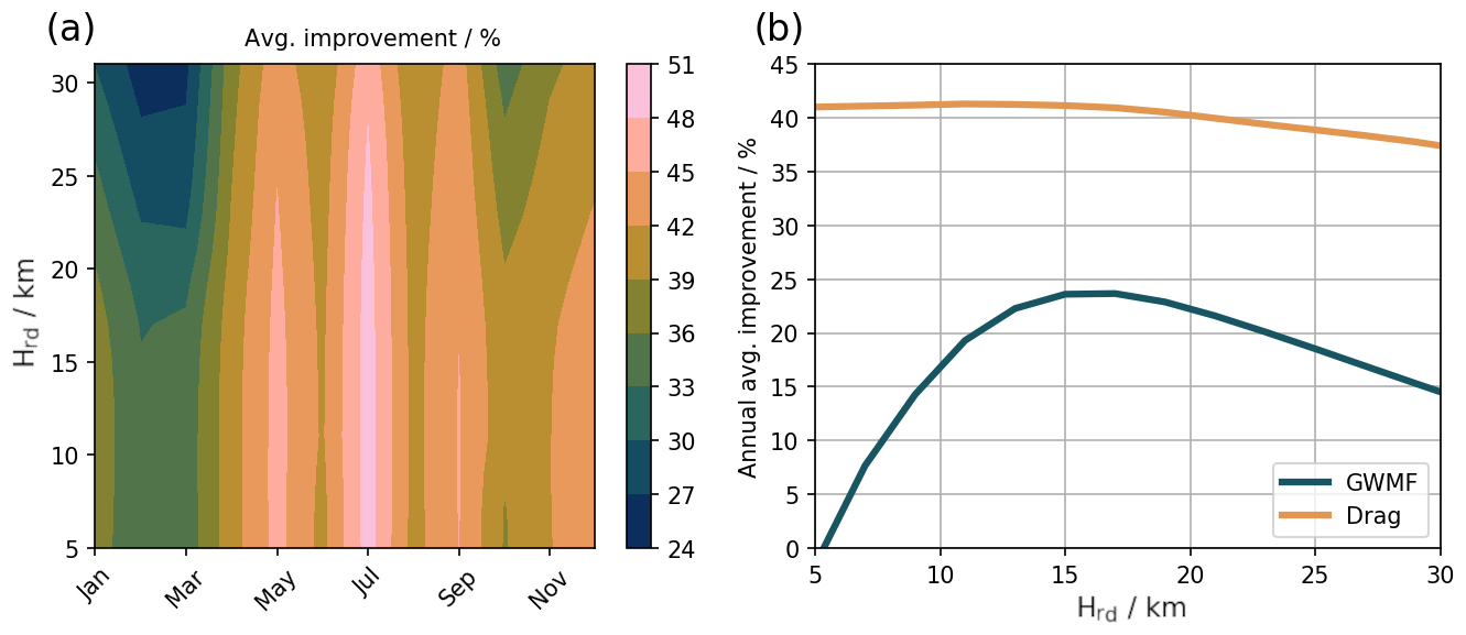
Figure 4(a) Improvement of GW drag across the year 2006 as monthly means for varying Hrd. The improvement is the reduction in deviation from REF through GW redistribution. (b) Annual mean improvement for GWMF (blue) and GW drag (orange) with varying Hrd.
In the present study, we use the redistribution maps described in Sect. 2 in the ECHAM/MESSy (European Center HAmburg Model/Modular Earth Submodel System) Atmospheric Chemistry (EMAC Jöckel et al., 2005, 2010, 2016) model. ECHAM (ECMWF Hamburg) is a global atmospheric GCM describing dynamics and comprising parameterisations for physical processes (Roeckner et al., 2003, 2006). MESSy is a framework for standardised implementation of Earth system models with flexible complexity, providing an infrastructure with generalised interfaces for coupling ESM components. The MESSy community policy and coding standard enable all users to optionally use all new developments, including those described in the present paper. Moreover, the flexible structure of MESSy allows transferring the developments to base models other than ECHAM. The standard model resolution for our purposes is T42L90MA, which corresponds to a resolution of ∼ 2.8∘ × 2.8∘ in latitude and longitude of the corresponding quadratic Gaussian grid and 90 layers in the vertical. In this setup, the uppermost level is located around 0.01 hPa and middle-atmospheric dynamics (MA) are explicitly resolved. In all simulations presented here, only the basic MESSy submodels for dynamics, clouds and diagnostics are applied. In the CCM EMAC, the submodel “OROGW” comprises the subgrid-scale orography (SSO) scheme, including the OGW parameterisation. OROGW is the central part for the implementations of the GWMF redistribution described next.
3.1 Implementation
As stated above, lateral propagation of GWs cannot be cost-efficiently computed in state-of-the-art GCMs due to the communication overhead between grid boxes in the horizontal. The separation and parallelisation of computation of different model domains on different computing tasks result in high cost and time for communication between (adjacent) grid cells. Hence, the idea is to apply the global GW redistribution only at one single altitude level, which shall account for the entire horizontal propagation of all GWs. Although this is a crude approximation, it is an important step towards a better representation of GW drag in the middle atmosphere. As described in Sect. 2.4, the ideal altitude for the GW redistribution is approximately 15 km, i.e. around 120 hPa. In the L90MA setup used here, the closest (hybrid sigma-pressure) model level to this altitude is level 65. This means that when the GW redistribution in EMAC is active, levels 90 (bottom) to 66 still use the ordinary columnar OGW scheme; GW redistribution happens in level 65, and in levels 64 to 1 (top), the redistributed GW fluxes are again treated by the columnar approach.
The submodel OROGW in EMAC comprises the OGW parameterisation by Lott and Miller (1997) and Lott (1999), which is described by Roeckner et al. (2003) for its use in ECHAM. In this scheme, GWMF τ (i.e. the Reynolds stress) in the level above the low-level breaking layer is launched by
where ρH, UH and NH are the incident density, zonal wind component and Brunt–Väisälä frequency at the launching height H, respectively; G is the GW parameter, which tunes the GWMF and has its default value set to 0.8; ν and σ are the standard deviation and the slope of the SSO, respectively; Zeff is the effective mountain height determined by the mountain height above the blocked flow; and is the directional vector determining the angle between the incident flow and the normal orographic ridge direction. This GWMF is calculated from the bottom upwards until either a critical level is encountered, leading to full deposition of GWMF, or partial GW breaking due to saturation happens.
The implementation of the OGW flux redistribution described below is schematically depicted in Fig. 5. Some EMAC/MESSy-specific implementation details are further provided in the Supplement.
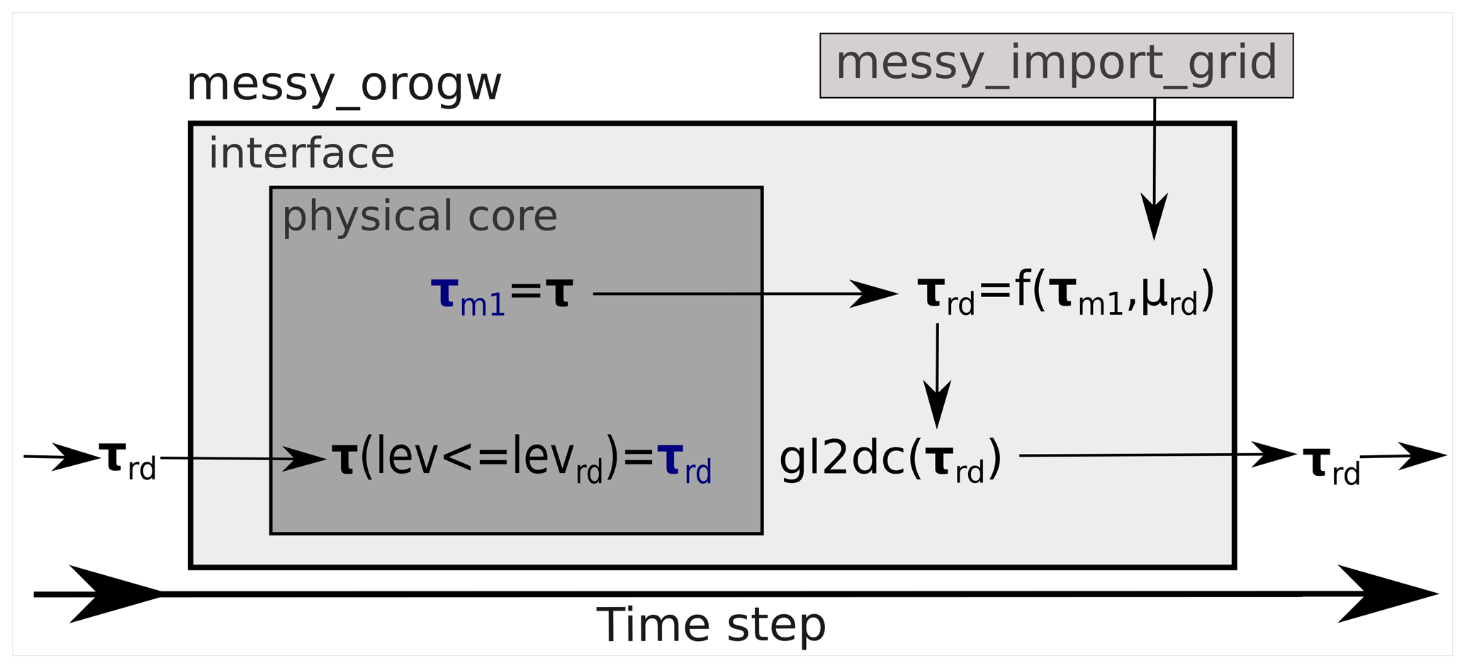
Figure 5Schematic of the GW redistribution implementation in the EMAC submodel OROGW. The physical core denotes the parameterisation itself, and the interface is the connection to the other model parts. Here, gl2dc stands for global to decomposition, μrd for the redistribution (rd) function, m1 for the minus 1 (with respect to the time step) value, lev for model level and τ for the GW flux. See main text for more explanations and the Supplement for EMAC/MESSy-specific implementation details.
In order to perform the redistribution, first τ at the redistribution level (here 65) is transferred from the physical core to the interface, where it can be processed further. This τ will be the basis for the redistributed flux. As this will happen in the subsequent time step, it is called τm1, where m1 stands for time step minus 1. At the end of the time step, global fields are generated by looping over the processing elements that are determined by the decomposition. This allows redistribution of τm1 globally to yield the redistributed τrd by
where is the redistribution map that was described in Sect. 2.3, and the subscripts tar and src denote (horizontal) target and source grid cell of the GWs at the level of redistribution, respectively. The four-dimensional redistribution map (two latitudes and two longitudes plus a possible time dimension) is read in via IMPORT_GRID (Kerkweg and Jöckel, 2015), which has been extended for the application of four-dimensional arrays (plus time axis) for this purpose. Next, a function (gl2dc) is applied to transpose τrd from a global field to a field in the simulation-specific decomposition. This function comprises the major part of the redistribution-caused overhead relating to total required computing time and memory loading on individual compute tasks, which will be further investigated in Sect. 3.3. τrd is then used in the subsequent time step to override τ in the level of redistribution and above before computation of wave breaking.
Wave breaking occurs when the critical Richardson number of 0.25 is reached. In this case, GWs are assumed to saturate, meaning that their amplitude is reduced to the value at which instability occurs (Lindzen, 1981). For this, in the parameterisation the saturated flux is calculated by
Here, Zoro contains parameters describing the wave properties at launch level. In the columnar approach, these values always refer to the same grid cell. However, when applying the GW redistribution, the launch level properties have to be communicated to the new location to which the GWMF was distributed. Otherwise, for example in grid boxes above the ocean, Zoro would be zero and thus lead to erroneous complete breaking of the waves. This means that for correct calculation of GW breaking after GW redistribution, Zoro has to be redistributed as well. However, in contrast to τ, Zoro is a (dynamic) parameter and not a variable that can be added up. Therefore, Zoro has to be normalised by the sum of all contributing entries of the redistribution map to account for the fraction of the parameter from a particular source box. Hence, redistributed Zoro is calculated by
As GW drag is computed by the GW flux difference between the level in question and the level below, loss and gain of GW flux through redistribution would lead to erroneous GW drag. Therefore, wave breaking and computation of GW drag needed to be disabled at the level of redistribution. Consequently, no GW drag can appear at this model level. This technically needed simplification should be kept in mind when analysing the results. Another option could be to fill this level with the drag of the level below or above. However, the effect of OGW drag at the redistribution altitude (∼ 15 km) is generally relatively low in comparison to other effects. Therefore, the level without OGW drag does not generate any inconsistencies in the dynamical fields in our simulations, which gives us confidence that the chosen approach is applicable.
3.2 Updating the subgrid-scale orography
During conduction of the first test simulations with the GW redistribution, we identified deficiencies in the SSO representation in EMAC. In particular, we found the continental edges to be underrepresented in the standard SSO. This means that in comparison with the ridge parameterisation in GROGRAT, GW launching does not happen in grid boxes at the continental edges in EMAC. The MWM shows strong lateral propagation, especially by MWs from these regions.
In order to achieve a better representation of MW launching in EMAC, we therefore updated the SSO by means of the same ETOPO1 (Amante and Eakins, 2009) topography data used for the ridge parameterisation in Sect. 2.2. While the original SSO data used in EMAC are based on a US Navy (10′ × 10′) data set (see Wallace et al., 1983), the new parameters are derived from the high-resolution 1′ × 1′ ETOPO1 data. Mean elevation, standard deviation, peaks (maximum) and valleys (minimum) were derived directly from the topography data within the corresponding model grid cells. The other three required parameters for the parameterisation, namely anisotropy, slope and main orographic angle, can be derived from the former parameters based on the equations described by Lott and Miller (1997) and Baines and Palmer (1990). These are briefly repeated in the Supplement. Exemplarily, Fig. 6 shows the mean orography of the standard SSO and of the updated version for southern South America and the Antarctic Peninsula. For completeness, all SSO parameters are shown for this region in the Supplement (Figs. S1 and S2).
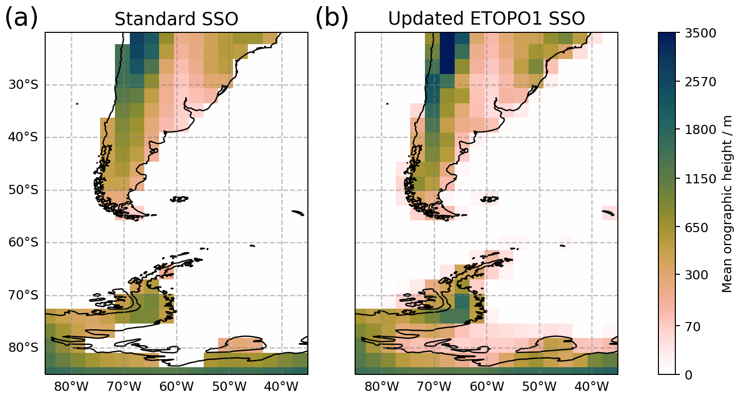
Figure 6Mean subgrid-scale orography elevation as used in (a) standard EMAC simulations and (b) as updated from ETOPO1 high-resolution topography data. For details see main text.
Figure 6 shows that the updated SSO is more nuanced than the standard one and, in particular, that the representation of orography is enhanced at the continental edges. The Antarctic Peninsula displays several grid boxes where no orography can be seen in the standard SSO, but the ETOPO1 SSO does show orographic elevation. Some of the smaller islands, e.g. South Georgia, also display SSO in the updated version, which might contribute to a more realistic description of GW drag in the polar vortex (see e.g. Perrett et al., 2021). In the model test simulations which will follow in Sect. 3.4, we will investigate how this SSO update affects GW flux and drag in the middle atmosphere.
3.3 Run time performance analysis
To assess the additional computing resources required to apply the GW redistribution in EMAC, we performed 10 dedicated simulations over 1 simulation month. Five of these simulations were carried out with the GW redistribution activated (Red.) and the other five without (Col.). The respective five simulations differ by usage of the number of compute tasks; i.e. 64, 128, 256, 512 and 1024 tasks are used. See the Supplement (Table S1) for specific usage of the associated decomposition in these simulations. We performed the simulations on HLRE-4 (levante) at the German Supercomputing Climate Center (DKRZ). The standard nodes of this high-performance computer feature 128 tasks per node, and hence our simulations used 0.5, 1, 2, 4 and 8 compute nodes, respectively. In these simulations, only the very basic setup for model dynamics and physics is activated. Moreover, all model output, except for the run time analysis output (QTIMER), which only outputs once at the end of the month, is switched off to assess the relative effect of only the model performance itself without any additional output. Figure 7 shows run time and required node hours (node-h) of the 10 simulations. Note that due to the output design, the first time step, which includes the build-up of the model including read-in of the redistribution map, has to be considered in this analysis; however, our tests have shown that this does not substantially influence the model run time evaluation presented here.
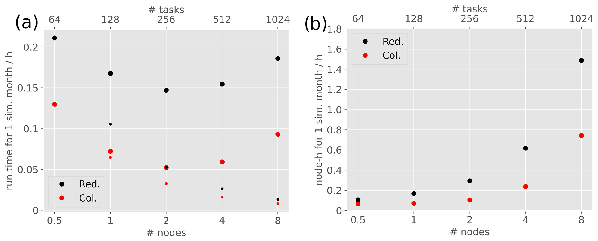
Figure 7(a) Run time and (b) required node hours for 1 simulation month in five simulations with (Red. for redistribution) and five simulations without the GW redistribution (Col. for columnar). The simulations were performed using 0.5, 2, 4 and 8 compute nodes. The small dots in panel (a) denote the theoretical run time for optimal scaling based on the 64-task simulation.
The run time analysis (Fig. 7a) shows that in both cases, i.e. with and without the GW redistribution, run time decreases with an increasing number of compute tasks used until usage of two nodes. Between using two and four nodes, the run time starts increasing again. This is a computer-specific behaviour and depends on the relation between bandwidth and tasks. In the spectral GCM EMAC, it is mainly the grid point space to spectral space transposition that requires communication between all tasks at each time step. The absolute run time difference between the two simulation types remains similar with an increased number of utilised compute tasks. However, in the case with redistribution, run time deviates from optimal scaling more strongly with increasing use of tasks. This is mainly due to the additional all-to-all communication during use of the gl2dc function that was described in Sect. 3.1. Using only 64 tasks, run time with GW redistribution increases by a factor of around 1.7 (67 %) and using 256 tasks (two nodes) by a factor of 2.8 (184 %). As general scaling performance of EMAC diminishes when using even more nodes, the relation improves again in that direction. When we performed these tests on the HLRE-3 (mistral), which was discarded in the year 2022 and featured 36 tasks per node, scaling of standard EMAC did not diminish even when using 16 nodes (576 tasks). On mistral, the run time overhead factor with OGW redistribution was 1.2 (17 %) with 1 node and 2.1 (111 %) with 16 nodes. The required node hours for 1 simulation month with and without GW redistribution (Fig. 7b) generally show an increase with an increasing number of tasks. As this measure generally represents the run time scaled with the number of nodes, the relations between the two simulations are the same as above. Additionally, excessive memory load on individual compute nodes might become an issue due to the all-to-all communication. We have not faced any problems with regard to this on the mistral and levante supercomputers at the DKRZ, but usage of finer resolution could lead to complications in that regard depending on the supercomputer architecture.
If we consider that activating the interactive chemistry mechanism MECCA in EMAC (Sander et al., 2019) including numerous tracers, or using the model in a setup with coupled deep ocean, can increase the required node hours by more than an order of magnitude, the overhead of the GW redistribution can be regarded as moderate. Hence, for the current EMAC this can be a feasible solution for improving the GW representation; however, for highly parallel model designs a different solution must be sought. Overall, we conclude that chemistry–climate simulations including the GW redistribution with the state-of-the-art EMAC model are affordable and shall be the aim to achieve a better representation of OGWs (which will be shown in the remainder of this paper). Multi-decadal chemistry–climate simulations with fine enough resolution to disable physical parameterisations such as GWs or convection (which is <1 km horizontal resolution; see Polichtchouk et al., 2022; Kruse et al., 2022) are unlikely in the foreseeable future, and other approaches, such as integrated ray tracers in CCMs, are yet to be fully developed and strongly enhance computing time too. Hence, the GW redistribution can be advantageous for ample time into the future, in which reliable climate projections are key for policy making. However, careful handling of the computing conditions in relation to the redistribution is needed.
3.4 GW flux and drag in EMAC test simulations
For a first evaluation of the GW redistribution in EMAC, we conducted test simulations for July 2006 in the T42L90MA resolution. This is the same period as investigated in the companion paper validating the MWM (Rhode et al., 2023). For this, the greenhouse gases, sea surface temperatures and the sea ice concentrations are prescribed. The simulations are purely dynamical; i.e. no chemistry is activated. Figure 8 shows monthly mean GWMF and zonal GW drag of these test simulations with the standard columnar OGW scheme and with GW redistribution. Here, we chose the redistribution map that was generated particularly for July of 2006 (see Sect. 2.3). We focus mainly on the region around Patagonia and the Antarctic Peninsula, since OGWs are known to be influenced particularly strongly by lateral propagation there (see e.g. Rapp et al., 2021) and the impact of lateral propagation on dynamics is considered to be large in this region (see e.g. McLandress et al., 2012). For completion, a global depiction of GWMF at the level of GW redistribution is provided in Fig. S4.
The comparison of the OGWMF maps in Fig. 8a and b shows that through GW redistribution, GWMFs are generally more spread out. More precisely, there is less GWMF over the continents and over orography, while now there is GWMF over the oceans and other regions where no or only little orography is located. This agrees with findings in Fig. 2b and the expectations of the implementation and was one of the aims of the parameterisation refinement. GWMF over the ocean is mostly about 1 order of magnitude smaller than GWMF over land. Most of the GWMF over the ocean can be seen downwind from the Andes and the Antarctic Peninsula, which is consistent with findings from satellite observations (e.g. Ern et al., 2018; Hindley et al., 2020) and high-resolution modelling (e.g. Strube et al., 2021; Polichtchouk et al., 2022). Moreover, some meridional displacement takes place, which can clearly be seen by comparing panels c and d of Fig. 8. At model level 65, the chosen level of GW redistribution, some of the GWMF is being displaced meridionally and this reduces the GW gap at 60∘ S. Figure 8e and f show that the columnar sum of GW drag displays similar spatial patterns as the GWMF at level 65. This could be expected, as GW drag is closely related to the location and deposition of GWMF via breaking, which mostly takes place in the middle atmosphere. The comparison of Fig. 8g and h shows that the 60∘ S GW gap is partly closed in zonal-mean GW drag when GW redistribution is activated. Further, these figures also display larger zonal-mean GW drag in total for the redistributed case, in particular in the upper model layers. This is somewhat surprising and cannot be explained by details of the implementation, as the total GWMF is conserved in our approach. A possible reason is better vertical propagation conditions for the redistributed GWs, but see Sect. 3.5 where we discuss this point in more detail.
These results prove the technical applicability of our development and its potential to improve the horizontal distribution of OGWs in EMAC. However, regarding the redistribution maps from Sect. 2.3, we expected stronger lateral GW displacement through the GW redistribution in the zonal as well as in the meridional direction. Many of these far-away-propagating GWs in GROGRAT, however, seem to stem from regions at the continental edges, where no orography is present in the standard EMAC SSO, translating into a lack of GW sourcing in these grid boxes. Therefore, we next evaluate how the updated SSO from Sect. 3.2 influences the results by repeating for Fig. 9 the analysis from Fig. 8 but using the updated SSO.
Comparison of the panels in the left columns of Figs. 8 and 9 shows that the new SSO generally leads to enhanced launching of GWMF and subsequently stronger GW drag. In particular, the continental edges and, in addition, some of the small islands outside the displayed region have larger (or rather any) GWMF and drag with the new SSO. As expected, this also leads to more far-away transport of the GWMF (Fig. 9b). Considerable patches of GWMF and GW drag can now be seen further away from orography, downwind as far as at 20∘ W. Moreover, meridional displacement, especially into the latitudes of the Drake Passage, is now distinctly represented (see Fig. 9b and f) such that the 60∘ S gap is completely closed (see Fig. 9d and h). Again, the GW redistribution leads to more total zonal-mean GW drag, which will be discussed in the next section (compare Fig. 9g with h). Changes in GW drag directly impact winds and temperatures and indirectly impact planetary wave propagation (see e.g. Cohen et al., 2014; Eichinger et al., 2020; Šácha et al., 2021), thereby altering stratospheric dynamics. Even differences in GW asymmetry with consistent zonal-mean forcing can cause changes in dynamics (see Šácha et al., 2016; Samtleben et al., 2020; Kuchar et al., 2020). In the next section, we provide a brief analysis of the GW redistribution impact on Antarctic polar vortex dynamics.
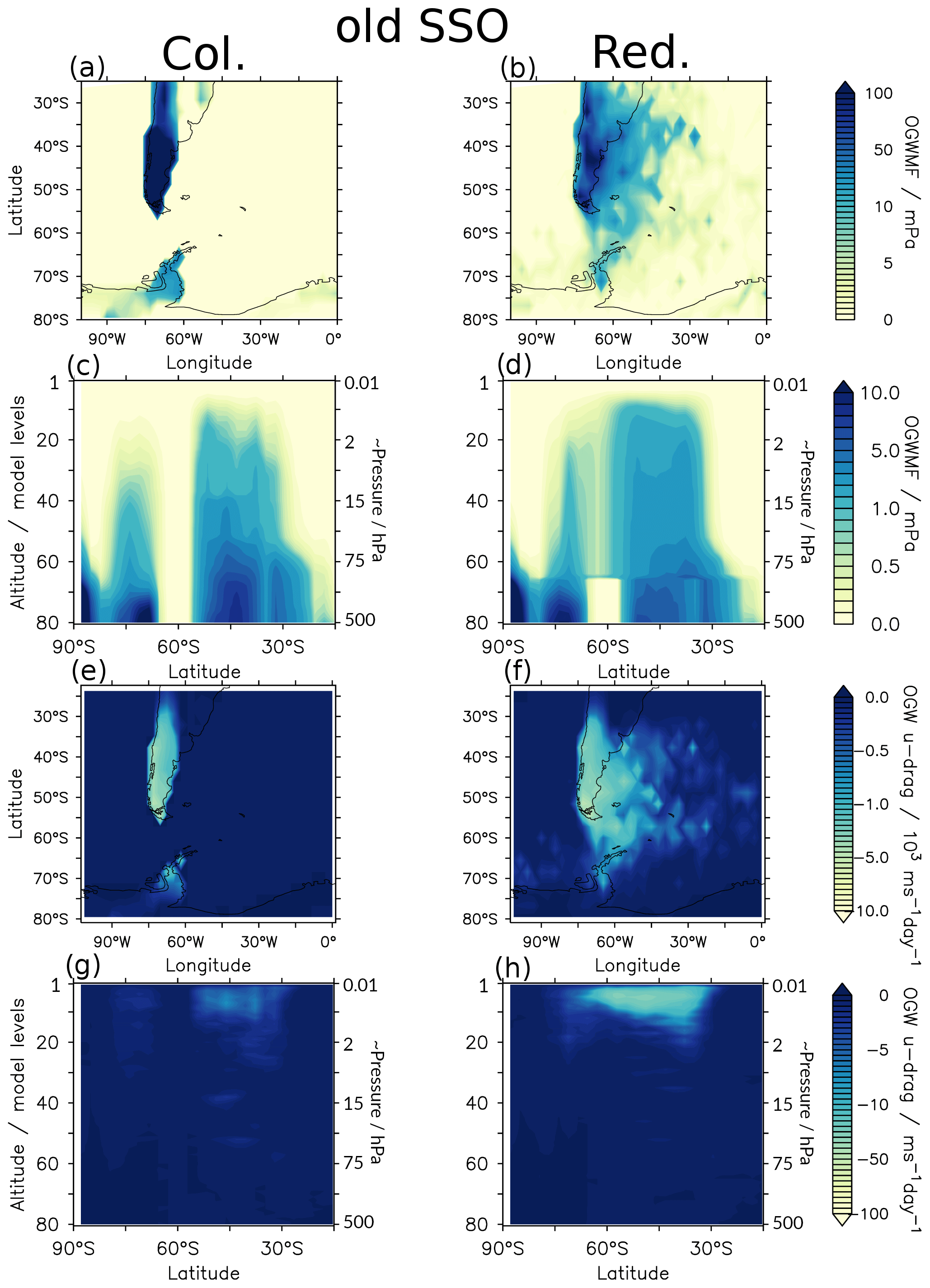
Figure 8Comparison of orographic GWMF and GW drag between the standard columnar approach (left) and using the GW redistribution (right) with the standard SSO: (a–d) GWMF at model level 65 (level of redistribution) (a, b) and as a zonal mean (c, d). (e–h) GW drag vertically summed up (e, f) and as a zonal mean (g, h). Note that panels (c), (d), (g) and (h) are depicted in hybrid sigma-pressure model levels to clearly visualise the redistribution level. For reference, the second vertical axis denotes approximated pressure levels, and additionally the distribution of hybrid sigma-pressure model levels of the EMAC L90MA setup with pressure altitude is shown in the Supplement.
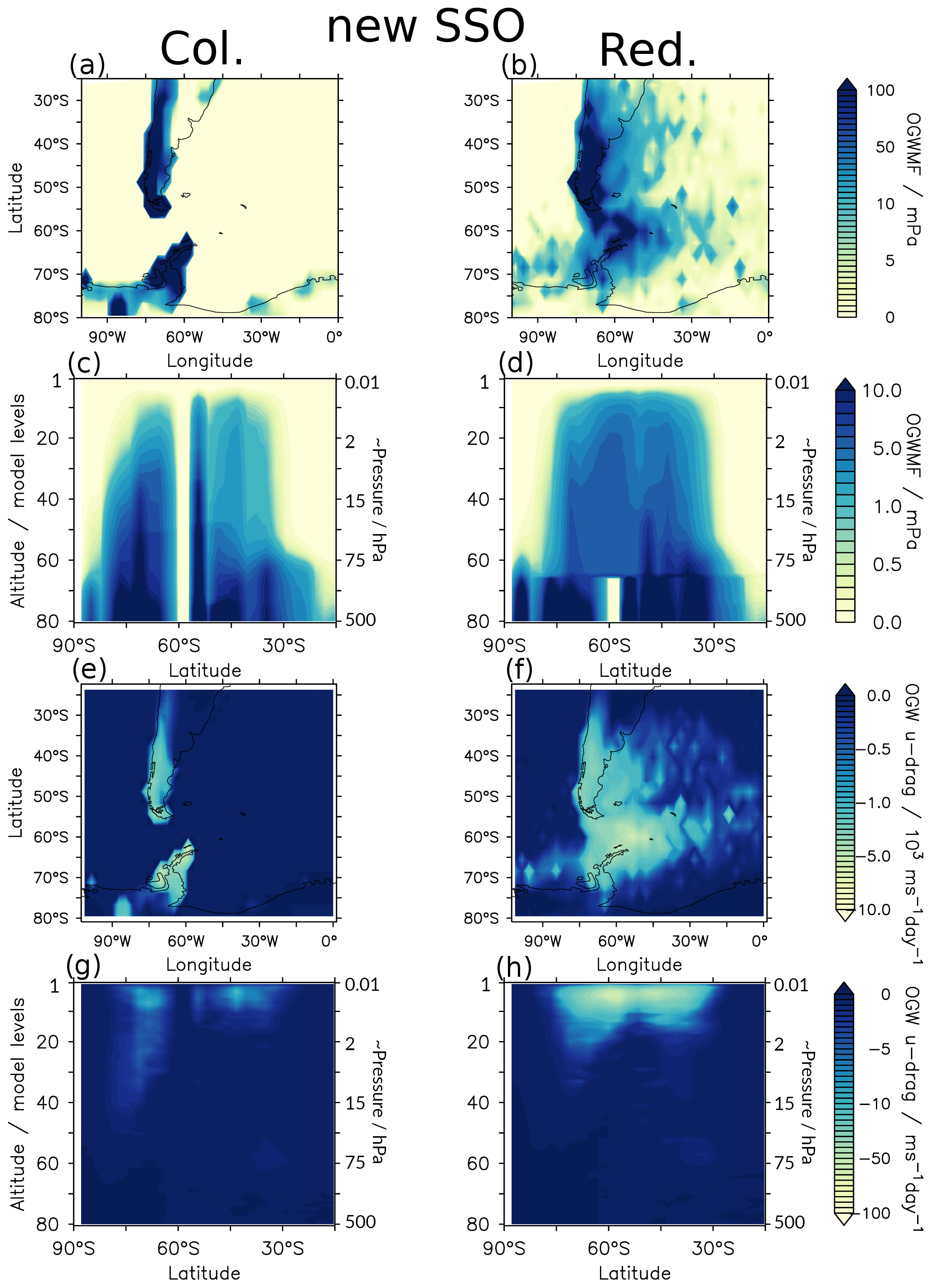
Figure 9As Fig. 8 but with the updated SSO.
3.5 Impacts on stratospheric polar vortex dynamics
To obtain a general picture of the impact of the OGW redistribution on stratospheric Antarctic polar vortex dynamics, we performed four time slice simulations over 25 years with sea surface temperatures and sea ice concentration boundary conditions from the year 2006 and prescribed GHGs. The four simulations are designed in the same manner as the test simulations in Sect. 3.4, with and without GW redistribution and using the new and the old SSO, respectively. The first 5 years of these simulations are considered spin-up and hence not analysed. The resolution again is T42L90MA and the output time step is 6 h. In contrast to the test simulations above, the redistribution functions used here are based on annual means for the year 2006 instead of the July 2006 maps (see Sect. 2.4), but they are still temporally constant.
To assess these simulations, we first analyse the Southern Hemispheric 20-year climatological zonal mean GWMF at 10 hPa during JJA. Figure 10 shows OGWMF and total GWMF (OGW + non-orographic (N)GW) for the four simulations.
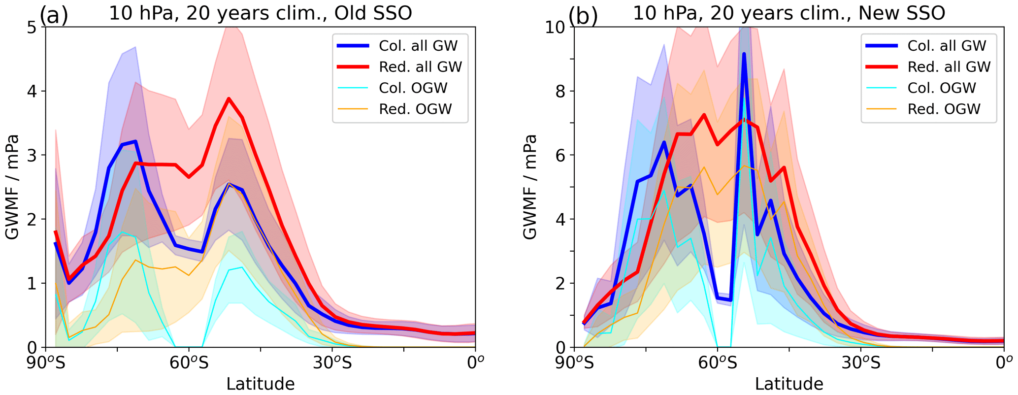
Figure 10Climatological 20-year JJA zonal-mean total GWMF and OGWMF at 10 hPa for the simulations with (a) the old SSO and (b) the new SSO. Col. stands for columnar and Red. for redistribution activated. The shading denotes the variability by means of 1σ of the GWMF.
The most obvious feature in Fig. 10 is that the GW gap at 60∘ S can be closed through OGW redistribution. This could already be seen in the previous section, but now we show that this is also the case for the climatological mean over austral winter and as conducted using an annual mean redistribution map rather than the specific July map. Using the old SSO (Fig. 10a), the redistribution enhances the total GWMF equatorward of around 70∘ S and reduces it poleward of this latitude. In the new SSO case (Fig. 10b), the general picture is similar, but due to more OGW excitation, GWMF is generally larger by about a factor of 2 (note the different scales in the two panels). Moreover, there is a spike with large OGWMF at ∼ 50∘ S in the columnar-only simulation that exceeds the redistributed case, likely due to GW launching from islands or continental edges. In the redistributed case, enhanced OGWMF can be seen here too, but the spike is smoothed out through GW redistribution. In general, the accumulated GWMF in the redistributed simulations exceeds the one from the columnar simulations at the 10 hPa level. Consequently, GW drag above 10 hPa is enhanced in the case with GW redistribution (see Fig. S9), consistent with results shown in Sect. 3.4. This behaviour could also be found in a ray-tracing experiment, where the drag increases at altitudes above 40 km and decreases between 25 and 30 km if horizontal propagation of GWs is permitted (not shown), and it was also found by Xu et al. (2017). As there is no feedback on the mean flow in the ray-tracing experiments, the changed propagation behaviour cannot be a result of background wind condition modifications through the GW changes. Rather, it must result from different propagation and/or dissipation conditions. One possible explanation could be a systematic GW redistribution to regions with more favourable propagation conditions for the GWs. A physical reason for this could be that around 60∘ S, where the zonal-mean wind maximum is located, the saturated GWMF given by Eq. (4) is larger, hence allowing GWs to propagate upwards without dissipating. This is supported by Plougonven et al. (2017), who reported large GWMF located at the jet maximum in observations and high-resolution simulations. Another systematic change through GW redistribution, however, is in the absolute GWMF values per grid cell at the redistribution level for most regions (see Figs. 9a, b and 8a, b). As our GW redistribution leads to a more spread-out distribution of GWMF, while conserving total GWMF at the redistribution level, it results in lower values per grid cell. Consequently, dissipation from saturation will occur only at higher altitudes (see Eq. 4), explaining why at 10 hPa GWMF is generally larger as a result of GW redistribution. Therefore, GWs generally propagate to higher altitudes through redistribution, and there they exert a stronger drag on the mean flow due to the scaling with inverse density.
The differences in GW drag that the altered GWMF translate to impact stratospheric dynamics via dissipation. To assess the impact on wind and temperatures, we show in Fig. 11 the climatological JJA zonal-mean zonal wind and temperature differences between the two simulations with and the two without redistributed OGWs for old and new SSO.
In the case with the old SSO (Fig. 11a, c), the zonal winds show clear signs of a stronger polar vortex poleward of 60∘ S and a weakened polar vortex equatorward of this latitude, indicating a poleward shift of the polar vortex. These signals might not be statistically significant here, but the monthly mean differences (see the Supplement) are partly significant and the signal is consistent from May through September. This indicates that high-latitude stratospheric dynamics are clearly influenced by OGW redistribution. These wind changes are generally consistent with a reduction of GWMF at high latitudes and enhanced GWMF north of about 70∘ S, as shown in Fig. 10. However, we expect that additional interaction between GWs, planetary waves and the mean flow (as analysed by e.g. Cohen et al., 2014; Eichinger et al., 2019; Šácha et al., 2021) additionally play a role for the response of the zonal wind to GW redistribution, constituting the well-known non-linearity of stratospheric dynamics. The polar temperature differences in this case, however, are small and barely significant. We performed a brief analysis of wave–wave interaction to analyse how the forcing by orographic, non-orographic and resolved waves reacts to the redistribution (see Fig. S10). As noted before, OGW drag strongly increases in the upper stratosphere. This increase is partly compensated for by a decrease in non-orographic GW drag and partly by planetary wave drag. However, we do not find a systematic compensation of the (missing) drag at 60∘ S as reported by Garcia et al. (2017). As shown by Eichinger et al. (2020), the occurrence of compensation, and thereby the impact on zonal winds, also seems to strongly depend on the background state, and in some cases amplifying effects are also found. An in-depth investigation of the wave–wave and wave–mean flow interactions will be needed to determine what exactly the crucial mechanisms are.
In the case with the new SSO (Fig. 11b, d), stronger winds can be seen throughout the polar vortex region when OGWMF is redistributed. This zonal wind signal is partly statistically significant in the individual boreal winter months (see Supplement), but the temperature signal in the high latitudes is robust even in the seasonal mean differences. The southern high-latitude lower stratosphere shows colder air and the higher stratosphere warmer air, and this is the case from April through September. This shows that in the case with the new SSO, the dynamical response to GW redistribution is somewhat different than in the case with the old SSO, and it cannot be explained by altered OGW forcing in the same manner. In principle, the abilities of GWs to propagate to higher levels as discussed above, resulting in reduced drag below around 10 hPa and enhanced drag above, are consistent with the temperature differences, and that again would be consistent with enhanced subsidence at lower altitudes and reduced subsidence above. However, the polar vortex strength also increases at levels above 10 hPa, where the total drag by OGWs is strongly enhanced (see Fig. S9). This again emphasises the non-linear nature of the response of high-latitude stratospheric dynamics to forcings, and an in-depth analysis of feedbacks between GWs, planetary waves and the mean flow would be necessary to gain a conclusive understanding of the modelled response to the GW redistribution. This includes its sensitivity to the background state (which Sigmond and Scinocca, 2010, showed to control wave propagation conditions and its sensitivity to changes) as indicated by the differences between the response in the new and old SSO case.

Figure 11Zonal-mean zonal wind (a and b) and temperature (c and d) differences in JJA between the simulations with and without OGW redistribution using the old (a and c) and the new (b and d) SSO. The contour lines show the climatologies without OGW redistribution in metres per second (m s−1) and degrees Celsius (∘C), respectively. Dotted regions depict where the differences are statistically significant at the 95 % level.
Another property of the Antarctic polar vortex that is of high interest is the day of the year of its breakdown (final warming). The persistence of the polar vortex through spring is relevant because of both ozone chemistry and its impact on tropospheric dynamics. In Fig. 12 we show the distribution of the stratospheric final warming day of the year for the four simulations. Following, for example, Black and McDaniel (2007) and de la Cámara et al. (2016), the final warming day of the year is diagnosed by using 5 d running means of daily data to calculate the final warming date as the last time that the zonal-mean zonal westerly wind at 60∘ S drops below 10 m s−1 until the subsequent autumn. Figure 12 shows that GW redistribution slightly shifts the mean of the final warming date to later times in the year, though this is barely statistically significant. With the old SSO, the median is shifted from day 298 to day 301 and with the new SSO from day 298 to day 303. In contrast to many other models, in EMAC the Antarctic polar vortex tends to break down too early (Jöckel et al., 2016) compared to reanalysis data (e.g. de la Cámara et al., 2016, found day ∼ 315 to be the median in ERA-Interim), and thus the redistribution acts to improve the model in this regard. Note that the structures of the final warming day distributions also change, in general towards a larger spread of the final warming date. These results are in line with the study by Gupta et al. (2021), who state that parameterised GW drag at 60∘ S generally provides more than half of the wind deceleration for the Antarctic polar vortex breakdown, and occasionally the amount can even be as high as the total necessary deceleration. Note further that the generally stronger OGWMF with the new SSO compared to the old one alters the final warming day distribution, but not its median value. As before, it will be of interest to study the interaction between GWs, planetary waves and the mean flow to more thoroughly understand this behaviour.
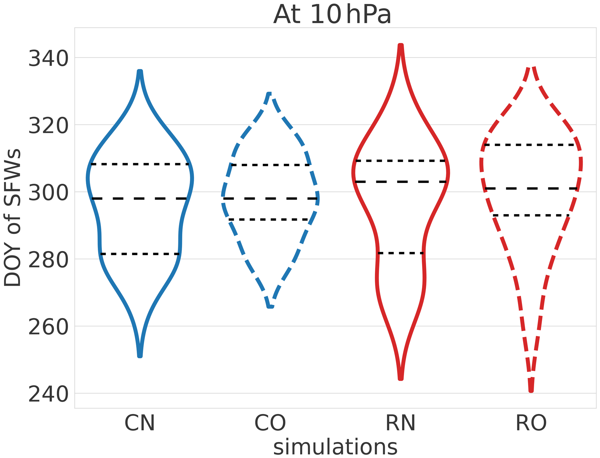
Figure 12Distribution of the day of the year (DOY) of the final stratospheric warming for JJA in the 20-year time slice simulations. The different simulations are denoted by C for columnar, R for redistribution, N for new SSO and O for old SSO. The horizontal dashed lines mark the quartiles.
For additional investigation of the Antarctic polar vortices in the four simulations, we use geometric-based methods by taking two-dimensional moments of dynamical fields. These diagnostics were, for example, put forward by Mitchell et al. (2011) and Seviour et al. (2013) and include the vortex excess kurtosis, aspect ratio and centroid latitude. The excess kurtosis is a non-linear and state-dependent diagnostic (see Matthewman and Esler, 2011); it is a measure of the departure of the vortex shape from an ellipse (Scott, 2016). Positive kurtosis values correspond to an eye shape with the vortex narrowing at its extremities, and larger positive values could be associated with higher probability of filamentation events of vortex material into the surf zone (Mitchell et al., 2012; Scott, 2016). GW redistribution enhances the kurtosis median at 10 hPa by around 10 % in both cases (see Fig. S11 for distribution). This can mean a significant change in circulation, but detailed analyses need to be conducted to draw clear conclusions here. The vortex aspect ratio median and distribution at 10 hPa are clearly changed through GW redistribution in the case with the new SSO, but not in the case with the old SSO (Fig. S12). A change in vortex form is in line with Fig. 11b and d. The centroid latitude does not reveal a clear picture as to any systematic changes through GW redistribution in our simulations (Fig. S13).
It has to be noted that some of the differences in the results are stronger between the (columnar approach) simulations with different SSOs than with or without redistribution. As the SSOs strongly alter GW launching and therefore GW drag, this is not surprising; however, as this measure does not change the spatial OGW distribution, which has been shown to be important for planetary-scale wave fields (Šácha et al., 2016, 2021; Samtleben et al., 2019, 2020), this does not help to simulate GW drag closer to reality. Moreover, this way, GWMF cannot be constrained to observations. In general, these results should be interpreted with caution, as the model has not been retuned. The scientific meaning of the results is therefore of a rather qualitative nature as to how much potential for changes in large-scale dynamics the new developments actually have. It remains to be shown if these signals are robust in various simulations with modified parameters and also with various horizontal and vertical resolutions. Different redistribution maps can be applied, and the redistribution altitude can be varied, possibly even implemented dynamically, or the regular tuning parameters of the OGW scheme can be customised. For this, a concrete idea for tuning these new model developments needs to be applied, and we lay out a plan for this in the following section.
In this paper, we describe a simplified solution of a three-dimensional orographic gravity wave (OGW) representation in the global chemistry–climate model (CCM) EMAC (Jöckel et al., 2010). The lack of horizontal OGW propagation constitutes a long-standing problem in atmospheric modelling, potentially with substantial impacts on middle-atmospheric dynamics that are crucial for accurate climate projections (McLandress et al., 2012; Geller et al., 2013).
As horizontal communication in general circulation models (GCMs) is computationally expensive, the idea is to implement a cost-efficient emulation of lateral OGW propagation. This is realised by redistributing orographic GWMF at one single altitude through use of tailor-made redistribution maps. The ray-tracing model GROGRAT coupled to a mountain ridge parameterisation (see Rhode et al., 2023) is applied to generate these maps. The latter are four-dimensional probability functions describing GW redistribution via horizontal propagation as a mapping from a source latitude–longitude grid to a target latitude–longitude grid (therefore the four dimensions are source latitude and longitude as well as target latitude and longitude). The individual map value depends on the relative fraction of the total GWMF in the given source cell that has been transported to the corresponding target grid box. The target altitude is one of the free parameters of the redistribution and was determined here to provide best results for 40 km, which results in an optimal approximation of horizontal GW drag redistribution. The ideal altitude for GW redistribution in the CCM was determined to be at 15 km, corresponding to around 120 hPa. For this, the GW redistribution was inferred from the ray-tracing model data, and the deviation from the setup with full four-dimensional (three spatial dimensions and time) propagation in the monthly mean was analysed. Both redistribution and target altitude can be the subject of further studies and in practice might be adjusted depending on the particular question of the given study, but here, we seek the most general solution. Additionally, the GW redistribution maps can be time-varying, generated by using annual means or monthly means of particular years or of averages over several years, and the meteorological boundary conditions can be taken from reanalyses or from model simulations. All these different options should, for now, be chosen depending on the science question(s) to be answered. It is worth mentioning, however, that a good approximation for individual months can already be gained from an annual mean redistribution pattern. Therefore, a major part of the horizontal GW propagation can be described by a general pattern. In the long run, a flow-dependent redistribution function might be sought in order to provide full flexibility of the model and higher accuracy in the propagation approximation. This could be realised by analysing the dominant modes of the time-varying redistribution function and their relation to variability in the large-scale flow. Possibly, the redistribution in a certain region, or even in a hemisphere, can be described by a few (up to three) leading modes. Online calculation in the GCM of the weights for the superposition of the dominant redistribution mode could then be the basis for the flow-dependent GW redistribution.
The implementation in the CCM EMAC works such that GW redistribution is applied at a specific model level, which can freely be chosen. To be closest to 15 km altitude with this, we chose model level 65 here for the L90MA setup used. Below the GW redistribution level, EMAC still comprises the ordinary columnar OGW scheme. Above this level, the redistributed GWMF again is treated as in the columnar approach, but now partly in other columns. The basis for this is the standard OGW parameterisation in EMAC, i.e. the scheme that was initially implemented by Lott and Miller (1997) and Lott (1999). As in this scheme, several incident quantities and parameters from the subgrid-scale orography (SSO) are required for calculating the saturated GWMF after wave breaking, and an additional variable (Zoro) comprising these quantities has to be redistributed. After performing the horizontal redistribution of the GWMF on global fields by looping over the blocks of the decomposition, transposition of these fields to the decomposition is performed. This allows usage of the redistributed fields in output and in the next time step and makes the implementation independent of the simulation-specific decomposition. Amemiya and Sato (2016) implemented three-dimensional propagation into the GCM MIROC (Model for Interdisciplinary Research on Climate; Watanabe et al., 2008) by means of including discretised ray-tracing equations. To our knowledge, however, this implementation only works in a specific decomposition and hence may not be suitable for operational use in CCM simulations.
Our analyses show that the computational overhead of the GW redistribution in EMAC is moderate. The main factor increasing communication time and consumption of node hours is the additional transposition of the global fields to the decomposition, where the entire information of the redistribution has to be present on each processing element. This enhances the overhead with increasing usage of computing tasks, such that a factor of 2–3 in node hours requirement is reached when the model is run on 200 to 500 compute tasks. This means that for highly parallel model designs, this approach is not feasible. For that, a model-integrated ray tracer with a communication approach between the neighbouring grid boxes or simply running the model at GW-allowing resolution might be more practicable strategies. At present, however, such approaches are far too costly for multiple decadal or centennial simulations (in particular when including comprehensive chemistry), and computing resources (computing and data storage facilities) are not growing quickly enough to provide such possibilities in the near future. This is particularly true, as for climate projections it is not one “true” simulation that is needed, but instead an ensemble of simulations with different settings, models and scenarios. For current EMAC chemistry–climate simulations, which are usually run on around 400–500 tasks on state-of-the-art high-performance computing systems, the GW redistribution as presented here is absolutely viable. In particular, in comprehensive CCM simulations (including the chemical mechanism, numerous tracers and possibly a coupled ocean model) the GW redistribution overhead will be a minor part of the computing time consumption.
First EMAC test simulations with this new implementation show that the GWMF is generally more spread out and also extends over the ocean when the GW redistribution is activated. In particular, some GWMF is located downwind from the Andes and the Antarctic Peninsula, as expected from high-resolution modelling (Strube et al., 2021; Polichtchouk et al., 2022) and satellite observations (Ern et al., 2018; Hindley et al., 2020). Moreover, meridional displacement of the GWMF at the level of redistribution to some degree closes the well-known GW gap at 60∘ S in the CCM. Our simulations show a larger total zonal-mean GW drag above ∼ 10 hPa when the GW redistribution is active and less GW drag below. By implementation design, the total GWMF is globally conserved when applying the GW redistribution; this is hence an indirect effect, which is also reproduced in ray-tracing experiments. Most likely, the propagation to higher altitudes results from lower values of GWMF per grid cell, so that saturation is reached only at higher levels, and from more favourable vertical propagation conditions around the polar night jet where some GWMF has been redistributed.
We also show that the GWMF and drag results improved considerably by using an updated SSO, especially because GWMF that is zonally transported far away from its source was underrepresented with the standard SSO. The reason is that in GROGRAT, GWs that are excited at the continental edges experience strong lateral propagation and the standard EMAC SSO does not feature any mountains there. With the new SSO, meridional displacement also increases, leading to a complete closure of the GW gap at 60∘ S.
The OGW redistribution has impacts on the representation of stratospheric dynamics, in particular on the Antarctic polar vortex with implications for Antarctic stratospheric ozone and its trends. The results of Amemiya and Sato (2016) also show an alleviation of the 60∘ S gap. However, they could not find considerable changes in the polar night jet, possibly due to compensation mechanisms with planetary waves (see e.g. Cohen et al., 2014; Sigmond and Shepherd, 2014; Eichinger et al., 2020). Our simulations, in contrast, show that significant differences in structural zonal-mean zonal wind patterns can be generated through the OGW redistribution, and this can translate into robust high-latitude temperature changes. In contrast to most CCMs, EMAC comprises a warm pole bias in the Southern Hemisphere (Jöckel et al., 2016), which means that the cooling in the lower stratosphere simulated here through OGW redistribution signifies an improvement of this bias, with the potential to advance the representation of polar ozone. A shift of the final Antarctic polar vortex breakdown to later days in the year could also be detected in the simulations, which corresponds to results by Gupta et al. (2021), who found a large contribution of parameterised GW drag at 60∘ S for the wind deceleration at the end of austral winter in ERA5 data. Moreover, specific diagnostics of the vortex geometry, i.e. excess kurtosis, aspect ratio and centroid latitude, reveal that clear changes in the polar vortex geometry occur, which has implications for its stability and thereby stratospheric warming frequency. In further consequence, this can have large impacts on the simulation of stratospheric polar ozone in the model, i.e. the representation of the ozone hole, and the simulated ozone recovery across the 21st century. Therefore, it should be of high interest to consolidate these new developments for further use in simulations with enabled interactive chemistry to perform and analyse climate projection simulations with redistributed GWMF. This could include analysis of the GW redistribution impacts in a changing climate concerning investigations of GW hotspots, stratospheric warmings, polar vortex strength and variability, ozone chemistry, and downward coupling and interactions between GWs and planetary waves on various temporal and spatial scales.
Refinements of the GW parameterisations in GCMs are increasingly important for climate modelling, partly because more and more knowledge is still being gathered about GWs that needs to find its way into the schemes (see Plougonven et al., 2020). But also, as the resolution of model simulations tends to increase, more (but not all) of the GW spectrum becomes resolved and the parameterisations have to be revised. On that account, it will become even more important to be aware of the possibilities lingering in the depths of the schemes and to have the parameterisations as close to the physics as possible. For this, testing the GW redistribution in other horizontal and vertical resolutions in order to assess their resolution dependency and whether the modifications have to be designed in a scale-aware manner will be important. Moreover, revisiting the free parameters described above of the redistribution (and analysing how the impact of redistribution varies with climate change) and of the GW scheme itself will be an interesting task. On that note, the importance of a second, or a dynamical, altitude of redistribution should also be assessed. However, the next step for consolidation of this development will have to be elaborate model tuning. This could now be conducted in a novel manner, i.e. not by using the GW scheme to tune the model to a certain climatic state, but by directly constraining the GWMF to those of high-resolution simulations such as conducted by Polichtchouk et al. (2022) to satellite observations such as shown in Ern et al. (2018) and Hindley et al. (2020), as well as to high-resolution point observations, for example, by Kaifler and Kaifler (2021) and Reichert et al. (2021). This would imply a new relevance for GW schemes and allow more meaningful comparisons with observations. One important question of this will be whether horizontal GW propagation is the reason for model deficiencies in representing the Antarctic polar vortex and associated ozone chemistry, which can then lead to more confidence in simulating climate change across the upcoming decades.
The Modular Earth Submodel System (MESSy) is continuously further developed and applied by a consortium of institutions. The usage of MESSy and access to the source code are licensed to all affiliates of institutions which are members of the MESSy Consortium. Institutions can become a member of the MESSy Consortium by signing the MESSy Memorandum of Understanding. More information can be found on the MESSy Consortium website (http://www.messy-interface.org, MESSy, 2023). The code presented here is based on MESSy version 2.55.2 and will be available in the next official release (version 2.56). Access to the code used in the mountain wave model and GROGRAT is possible upon request to the authors.
The EMAC simulation results are archived at DKRZ, and these output data as well as those from the mountain wave model and GROGRAT simulations are available upon request to the authors.
The supplement related to this article is available online at: https://doi.org/10.5194/gmd-16-5561-2023-supplement.
RE, SR, HG and PPr designed the study. RE and SR wrote the paper. SR generated the redistribution maps, the GROGRAT analyses and the new SSO with support by PPr, RE and HG. RE implemented the redistribution in EMAC with help by PJ, AKe, BK and HG; conducted the GCM simulations; and analysed the results with support by AKu, HG and PPi. All authors helped with discussions and with revising the paper.
At least one of the (co-)authors is a member of the editorial board of Geoscientific Model Development. The peer-review process was guided by an independent editor, and the authors also have no other competing interests to declare.
Publisher's note: Copernicus Publications remains neutral with regard to jurisdictional claims in published maps and institutional affiliations.
The authors want to thank Inna Polichtchouk, Petr Sácha, Sabine Brinkop, Markus Geldenhuys and Chris Kruse for discussions and Robert Reichert as well as two anonymous reviewers for valuable comments on the paper. Moreover, we acknowledge usage of resources from the Deutsches Klimarechenzentrum (DKRZ, German Climate Computing Centre) granted by its Scientific Steering Committee (WLA) under project ID bd1022.
This study was funded by the German Ministry for Education and
Research (grant no. 01 LG 1907; project WASCLIM) as part of the
Role of the Middle Atmosphere in Climate (ROMIC) programme and
by the Czech Science Foundation under grant no. 21-20293J. AKu acknowledges support from the Deutsche Forschungsgemeinschaft under grant JA836/43-1.
The article processing charges for this open-access publication were covered by the German Aerospace Center (DLR).
This paper was edited by Andrea Stenke and reviewed by two anonymous referees.
Alexander, M. J., Geller, M., McLandress, C., Polavarapu, S., Preusse, P., Sassi, F., Sato, K., Eckermann, S., Ern, M., Hertzog, A., Kawatani, Y., Pulido, M., Shaw, T., Sigmond, M., Vincent, R., and Watanabe, S.: Recent Developments on Gravity Wave Effects in Climate Models, and the Global Distribution of Gravity Wave Momentum Flux from Observations and Models, Q. J. Roy. Meteor. Soc., 136, 1103–1124, https://doi.org/10.1002/qj.637, 2010. a, b
Amante, C. and Eakins, B.: ETOPO1 1 Arc-Minute Global Relief Model: Procedures, NOAA National Centers for Environmental Information [data set], https://doi.org/10.7289/V5C8276M, 2009. a, b
Amemiya, A. and Sato, K.: A New Gravity Wave Parameterization Including Three-Dimensional Propagation, J. Meteorol. Soc. Jpn., 94, 237–256, https://doi.org/10.2151/jmsj.2016-013, 2016. a, b
Andrews, D. G., Holton, J. R., and Leovy, C. B.: Middle atmosphere dynamics, vol. 40, Academic press, ISBN 9780120585762, 1987. a
Bacmeister, J., Newman, P., Gary, B., and Chan, K.: An algorithm for forecasting mountain wave-related turbulence in the stratosphere, Weather Forecast., 9, 241–253, https://doi.org/10.1175/1520-0434(1994)009<0241:AAFFMW>2.0.CO;2, 1994. a
Bacmeister, J. T.: Mountain-wave drag in the stratosphere and mesosphere inferred from observed winds and a simple mountain-wave parameterization scheme, J. Atmos. Sci., 50, 377–399, 1993. a, b
Baines, P. and Palmer, T.: Rationale for a new physically-based parametrization of subgrid-scale orographic effects, ECMWF Technical Memoranda, 169, 1–11, https://doi.org/10.21957/h4h36b3u, 1990. a
Baldwin, M. P. and Dunkerton, T. J.: Stratospheric harbingers of anomalous weather regimes, Science, 294, 581–584, https://doi.org/10.1126/science.1063315, 2001. a
Barry, R. G.: Mountain Weather and Climate, third edn., Cambridge University Press, Cambridge, UK, https://doi.org/10.1017/CBO9780511754753, 2008. a
Black, R. X. and McDaniel, B. A.: Interannual Variability in the Southern Hemisphere Circulation Organized by Stratospheric Final Warming Events, J. Atmos. Sci., 64, 2968–2974, https://doi.org/10.1175/JAS3979.1, 2007. a
Bretherton, F.: The propagation of groups of internal gravity waves in a shear flow, Q. J. Roy. Meteor. Soc., 92, 466–480, https://doi.org/10.1002/qj.49709239403, 1966. a
Brewer, A. W.: Evidence for a world circulation provided by the measurements of helium and water vapour distribution in the stratosphere, Q. J. Roy. Meteor. Soc., 75, 351–363, https://doi.org/10.1002/qj.49707532603, 1949. a
Charney, J. G. and Drazin, P. G.: Propagation of planetary-scale disturbances from the lower into the upper atmosphere, J. Geophys. Res., 66, 83–109, https://doi.org/10.1029/JZ066i001p00083, 1961. a
Cohen, N. Y., Gerber, E. P., and Bühler, O.: What drives the Brewer–Dobson circulation?, J. Atmos. Sci., 71, 3837–3855, 2014. a, b, c
de la Cámara, A., Lott, F., and Hertzog, A.: Intermittency in a stochastic parameterization of nonorographic gravity waves, J. Geophys. Res.-Atmos., 119, 11905–11919, https://doi.org/10.1002/2014JD022002, 2014. a
de la Cámara, A., Lott, F., Jewtoukoff, V., Plougonven, R., and Hertzog, A.: On the Gravity Wave Forcing during the Southern Stratospheric Final Warming in LMDZ, J. Atmos. Sci., 73, 3213–3226, https://doi.org/10.1175/JAS-D-15-0377.1, 2016. a, b
Dobson, G. M. B.: Origin and distribution of the polyatomic molecules in the atmosphere, P. Roy. Soc. Lond. A Mat., 236, 187–193, https://doi.org/10.1098/rspa.1956.0127, 1956. a
Eckermann, S. D. and Marks, C. J.: GROGRAT: A new model of the global propagation and dissipation of atmospheric gravity waves, Adv. Space Res., 20, 1253–1256, https://doi.org/10.1016/S0273-1177(97)00780-1, 1997. a, b
Eichinger, R., Dietmüller, S., Garny, H., Šácha, P., Birner, T., Bönisch, H., Pitari, G., Visioni, D., Stenke, A., Rozanov, E., Revell, L., Plummer, D. A., Jöckel, P., Oman, L., Deushi, M., Kinnison, D. E., Garcia, R., Morgenstern, O., Zeng, G., Stone, K. A., and Schofield, R.: The influence of mixing on the stratospheric age of air changes in the 21st century, Atmos. Chem. Phys., 19, 921–940, https://doi.org/10.5194/acp-19-921-2019, 2019. a
Eichinger, R., Garny, H., Šácha, P., Danker, J., Dietmüller, S., and Oberländer-Hayn, S.: Effects of missing gravity waves on stratospheric dynamics; part 1: climatology, Clim. Dynam., 54, 3165–3183, https://doi.org/10.1007/s00382-020-05166-w, 2020. a, b, c, d
Ern, M., Trinh, Q. T., Preusse, P., Gille, J. C., Mlynczak, M. G., Russell III, J. M., and Riese, M.: GRACILE: a comprehensive climatology of atmospheric gravity wave parameters based on satellite limb soundings, Earth Syst. Sci. Data, 10, 857–892, https://doi.org/10.5194/essd-10-857-2018, 2018. a, b, c
Fritts, D. C. and Alexander, M. J.: Gravity wave dynamics and effects in the middle atmosphere, Rev. Geophys., 41, 1003, https://doi.org/10.1029/2001RG000106, 2003. a
Fritts, D. C. and Rastogi, P. K.: Convective and dynamical instabilities due to gravity wave motions in the lower and middle atmosphere: theory and observations, Radio Sci., 20, 1247–1277, 1985. a
Fritts, D. C., Smith, R. B., Taylor, M. J., Doyle, J. D., Eckermann, S. D., Dörnbrack, A., Rapp, M., Williams, B. P., Pautet, P.-D., Bossert, K., Criddle, N. R., Reynolds, C. A., Reinecke, P. A., Uddstrom, M., Revell, M. J., Turner, R., Kaifler, B., Wagner, J. S., Mixa, T., Kruse, C. G., Nugent, A. D., Watson, C. D., Gisinger, S., Smith, S. M., Lieberman, R. S., Laughman, B., Moore, J. J., Brown, W. O., Haggerty, J. A., Rockwell, A., Stossmeister, G. J., Williams, S. F., Hernandez, G., Murphy, D. J., Klekociuk, A. R., Reid, I. M., and Ma, J.: The Deep Propagating Gravity Wave Experiment (DEEPWAVE): An Airborne and Ground-Based Exploration of Gravity Wave Propagation and Effects from Their Sources throughout the Lower and Middle Atmosphere, B. Am. Meteorol. Soc., 97, 425–453, https://doi.org/10.1175/BAMS-D-14-00269.1, 2016. a, b
Garcia, R. R., Smith, A. K., Kinnison, D. E., Álvaro de la Cámara, and Murphy, D. J.: Modification of the Gravity Wave Parameterization in the Whole Atmosphere Community Climate Model: Motivation and Results, J. Atmos. Sci., 74, 275–291, https://doi.org/10.1175/JAS-D-16-0104.1, 2017. a, b
Geller, M. A., Alexander, M. J., Love, P. T., Bacmeister, J., Ern, M., Hertzog, A., Manzini, E., Preusse, P., Sato, K., Scaife, A., and Zhou, T.: A comparison between gravity wave momentum fluxes in observations and climate models, J. Climate, 26, 6383–6405, https://doi.org/10.1175/JCLI-D-12-00545.1, 2013. a, b
Gerber, E. P., Butler, A., Calvo, N., Charlton-Perez, A., Giorgetta, M., Manzini, E., Perlwitz, J., Polvani, L. M., Sassi, F., Scaife, A. A., Shaw, T. A., Son, S.-W., and Watanabe, S.: Assessing and understanding the impact of stratospheric dynamics and variability on the Earth system, B. Am. Meteorol. Soc., 93, 845–859, https://doi.org/10.1175/BAMS-D-11-00145.1, 2012. a
Giorgetta, M. A., Manzini, E., and Roeckner, E.: Forcing of the quasi-biennial oscillation from a broad spectrum of atmospheric waves, Geophys. Res. Lett., 29, 86-1–86-4, https://doi.org/10.1029/2002GL014756, 2002. a, b
Gregory, D., Shutts, G. J., and Mitchell, J. R.: A new gravity-wave-drag scheme incorporating anisotropic orography and low-level wave breaking: Impact upon the climate of the UK Meteorological Office Unified Model, Q. J. Roy. Meteor. Soc., 124, 463–493, https://doi.org/10.1002/qj.49712454606, 1998. a
Gupta, A., Birner, T., Dörnbrack, A., and Polichtchouk, I.: Importance of gravity wave forcing for springtime southern polar vortex breakdown as revealed by ERA5, Geophys. Res. Lett., 48, e2021GL092762, https://doi.org/10.1029/2021GL092762, 2021. a, b, c
Hardiman, S. C. and Haynes, P. H.: Dynamical sensitivity of the stratospheric circulation and downward influence of upper level perturbations, J. Geophys. Res., 113, D23103, https://doi.org/10.1029/2008JD010168, 2008. a
Hersbach, H., Bell, B., Berrisford, P., Hirahara, S., Horanyi, A., Munoz-Sabater, J., Nicolas, J., Peubey, C., Radu, R., Schepers, D., Simmons, A., Soci, C., Abdalla, S., Abellan, X., Balsamo, G., Bechtold, P., Biavati, G., Bidlot, J., Bonavita, M., De Chiara, G., Dahlgren, P., Dee, D., Diamantakis, M., Dragani, R., Flemming, J., Forbes, R., Fuentes, M., Geer, A., Haimberger, L., Healy, S., Hogan, R. J., Holm, E., Janiskova, M., Keeley, S., Laloyaux, P., Lopez, P., Lupu, C., Radnoti, G., de Rosnay, P., Rozum, I., Vamborg, F., Villaume, S., and Thepaut, J.-N.: The ERA5 global reanalysis, Q. J. Roy. Meteor. Soc., 146, 1999–2049, https://doi.org/10.1002/qj.3803, 2020. a, b
Hindley, N. P., Wright, C. J., Hoffmann, L., Moffat-Griffin, T., and Mitchell, N. J.: An 18-year climatology of directional stratospheric gravity wave momentum flux from 3-D satellite observations, Geophys. Res. Lett., 47, e2020GL089557, https://doi.org/10.1029/2020GL089557, 2020. a, b, c
Hines, C. O.: A Modeling of Atmospheric Gravity Waves and Wave Drag Generated by Isotropic and Anisotropic Terrain, J. Atmos. Sci., 45, 309–322, https://doi.org/10.1175/1520-0469(1988)045<0309:AMOAGW>2.0.CO;2, 1988. a
Hitchcock, P. and Simpson, I. R.: The Downward Influence of Stratospheric Sudden Warmings, Q. J. Roy. Meteor. Soc., 71, 3856–3876, https://doi.org/10.1175/JAS-D-14-0012.1, 2014. a
Jöckel, P., Sander, R., Kerkweg, A., Tost, H., and Lelieveld, J.: Technical Note: The Modular Earth Submodel System (MESSy) – a new approach towards Earth System Modeling, Atmos. Chem. Phys., 5, 433–444, https://doi.org/10.5194/acp-5-433-2005, 2005. a
Jöckel, P., Kerkweg, A., Pozzer, A., Sander, R., Tost, H., Riede, H., Baumgaertner, A., Gromov, S., and Kern, B.: Development cycle 2 of the Modular Earth Submodel System (MESSy2), Geosci. Model Dev., 3, 717–752, https://doi.org/10.5194/gmd-3-717-2010, 2010. a, b, c
Jöckel, P., Tost, H., Pozzer, A., Kunze, M., Kirner, O., Brenninkmeijer, C. A. M., Brinkop, S., Cai, D. S., Dyroff, C., Eckstein, J., Frank, F., Garny, H., Gottschaldt, K.-D., Graf, P., Grewe, V., Kerkweg, A., Kern, B., Matthes, S., Mertens, M., Meul, S., Neumaier, M., Nützel, M., Oberländer-Hayn, S., Ruhnke, R., Runde, T., Sander, R., Scharffe, D., and Zahn, A.: Earth System Chemistry integrated Modelling (ESCiMo) with the Modular Earth Submodel System (MESSy) version 2.51, Geosci. Model Dev., 9, 1153–1200, https://doi.org/10.5194/gmd-9-1153-2016, 2016. a, b, c, d
Kaifler, B. and Kaifler, N.: A Compact Rayleigh Autonomous Lidar (CORAL) for the middle atmosphere, Atmos. Meas. Tech., 14, 1715–1732, https://doi.org/10.5194/amt-14-1715-2021, 2021. a
Kalisch, S., Preusse, P., Ern, M., Eckermann, S. D., and Riese, M.: Differences in gravity wave drag between realistic oblique and assumed vertical propagation, J. Geophys. Res. Atmos., 119, 10081–10099, https://doi.org/10.1002/2014JD021779, 2014. a
Kerkweg, A. and Jöckel, P.: The infrastructure MESSy submodels GRID (v1.0) and IMPORT (v1.0), Geosci. Model Dev. Discuss., 8, 8607–8633, https://doi.org/10.5194/gmdd-8-8607-2015, 2015. a
Kim, Y.-J., Eckermann, S. D., and Chun, H.-Y.: An overview of the past, present and future of gravity wave drag parametrization for numerical climate and weather prediction models, Atmos. Ocean, 41, 65–98, https://doi.org/10.3137/ao.410105, 2003. a
Kruse, C. G., Alexander, M. J., Hoffmann, L., van Niekerk, A., Polichtchouk, I., Bacmeister, J. T., Holt, L., Plougonven, R., Šácha, P., Wright, C., Sato, K., Shibuya, R., Gisinger, S., Ern, M., Meyer, C. I., and Stein, O.: Observed and Modeled Mountain Waves from the Surface to the Mesosphere near the Drake Passage, J. Atmos. Sci., 79, 909–932, https://doi.org/10.1175/JAS-D-21-0252.1, 2022. a, b, c
Kuchar, A., Sacha, P., Eichinger, R., Jacobi, C., Pisoft, P., and Rieder, H. E.: On the intermittency of orographic gravity wave hotspots and its importance for middle atmosphere dynamics, Weather Clim. Dynam., 1, 481–495, https://doi.org/10.5194/wcd-1-481-2020, 2020. a
Lindzen, R. S.: Turbulence and stress owing to gravity wave and tidal breakdown, J. Geophys. Res., 86, 9707–9714, https://doi.org/10.1029/JC086iC10p09707, 1981. a
Lott, F.: Alleviation of Stationary Biases in a GCM through a Mountain Drag Parameterization Scheme and a Simple Representation of Mountain Lift Forces, Mon. Weather Rev., 127, 788–801, https://doi.org/10.1175/1520-0493(1999)127<0788:AOSBIA>2.0.CO;2, 1999. a, b
Lott, F. and Miller, M. J.: A new subgrid-scale orographic drag parametrization: Its formulation and testing, Q. J. Roy. Meteor. Soc., 123, 101–127, https://doi.org/10.1002/qj.49712353704, 1997. a, b, c, d, e
Marks, C. and Eckermann, S.: A three-dimensional nonhydrostatic ray-tracing model for gravity waves: Formulation and preliminary results for the middle atmosphere, J. Atmos.Sci., 52, 1959–1984, https://doi.org/10.1175/1520-0469(1995)052<1959:ATDNRT>2.0.CO;2, 1995. a, b
Matthewman, N. J. and Esler, J. G.: Stratospheric Sudden Warmings as Self-Tuning Resonances. Part I: Vortex Splitting Events, J. Atmos. Sci., 68, 2481–2504, https://doi.org/10.1175/JAS-D-11-07.1, 2011. a
McLandress, C., Shepherd, T. G., Polavarapu, S., and Beagley, S. R.: Is Missing Orographic Gravity Wave Drag near 60∘ S the Cause of the Stratospheric Zonal Wind Biases in Chemistry-Climate Models?, J. Atmos. Sci., 69, 802–818, https://doi.org/10.1175/JAS-D-11-0159.1, 2012. a, b, c
Modular Earth Submodel System (MESSy): Homepage, http://www.messy-interface.org, last access: 26 September 2023. a
Mitchell, D. M., Charlton-Perez, A. J., and Gray, L. J.: Characterizing the Variability and Extremes of the Stratospheric Polar Vortices Using 2D Moment Analysis, J. Atmos. Sci., 68, 1194–1213, https://doi.org/10.1175/2010JAS3555.1, 2011. a
Mitchell, D. M., Charlton-Perez, A. J., Gray, L. J., Akiyoshi, H., Butchart, N., Hardiman, S. C., Morgenstern, O., Nakamura, T., Rozanov, E., Shibata, K., Smale, D., and Yamashita, Y.: The nature of Arctic polar vortices in chemistry–climate models, Q. J. Roy. Meteor. Soc., 138, 1681–1691, https://doi.org/10.1002/qj.1909, 2012. a
Palmer, T. N., Shutts, G. J., and Swinbank, R.: Alleviation of a systematic westerly bias in general circulation and numerical weather prediction models through an orographic gravity wave drag parametrization, Q. J. Roy. Meteor. Soc., 112, 1001–1039, https://doi.org/10.1002/qj.49711247406, 1986. a
Perrett, J. A., Wright, C. J., Hindley, N. P., Hoffmann, L., Mitchell, N. J., Preusse, P., Strube, C., and Eckermann, S. D.: Determining gravity wave sources and propagation in the southern hemisphere by ray-tracing AIRS measurements, Geophys. Res. Lett., 48, e2020GL088621, https://doi.org/10.1029/2020GL088621, 2021. a, b
Plougonven, R., de la Camara, A., Jewtoukoff, V., Hertzog, A., and Lott, F.: On the relation between gravity waves and wind speed in the lower stratosphere over the Southern Ocean., J. Atmos. Sci., 74, 1075–1093, https://doi.org/10.1175/JAS-D-16-0096.1, 2017. a
Plougonven, R., de la Cámara, A., Hertzog, A., and Lott, F.: How does knowledge of atmospheric gravity waves guide their parameterizations?, Q. J. Roy. Meteor. Soc., 146, 1529–1543, https://doi.org/10.1002/qj.3732, 2020. a, b
Polichtchouk, I., Wedi, N., and Kim, Y.-H.: Resolved gravity waves in the tropical stratosphere: Impact of horizontal resolution and deep convection parametrization, Q. J. Roy. Meteor. Soc., 148, 233–251, https://doi.org/10.1002/qj.4202, 2022. a, b, c, d
Preusse, P., Dörnbrack, A., Eckermann, S. D., Riese, M., Schaeler, B., Bacmeister, J. T., Broutman, D., and Grossmann, K. U.: Space-based measurements of stratospheric mountain waves by CRISTA, 1. Sensitivity, analysis method, and a case study, J. Geophys. Res., 107, 8178, https://doi.org/10.1029/2001JD000699, 2002. a
Rapp, M., Kaifler, B., Dörnbrack, A., Gisinger, S., Mixa, T., Reichert, R., Kaifler, N., Knobloch, S., Eckert, R., Wildmann, N., Giez, A., Krasauskas, L., Preusse, P., Geldenhuys, M., Riese, M., Woiwode, W., Friedl-Vallon, F., Sinnhuber, B.-M., de la Torre, A., Alexander, P., Hormaechea, J. L., Janches, D., Garhammer, M., Chau, J. L., Conte, J. F., Hoor, P., and Engel, A.: SOUTHTRAC-GW: An Airborne Field Campaign to Explore Gravity Wave Dynamics at the World’s Strongest Hotspot, B. Am. Meteorol. Soc., 102, E871–E893, https://doi.org/10.1175/BAMS-D-20-0034.1, 2021. a
Reichert, R., Kaifler, B., Kaifler, N., Dörnbrack, A., Rapp, M., and Hormaechea, J. L.: High-Cadence Lidar Observations of Middle Atmospheric Temperature and Gravity Waves at the Southern Andes Hot Spot, J. Geophys. Res.-Atmos., 126, e2021JD034683, https://doi.org/10.1029/2021JD034683, 2021. a
Rhode, S., Preusse, P., Ern, M., Ungermann, J., Krasauskas, L., Bacmeister, J., and Riese, M.: A mountain ridge model for quantifying oblique mountain wave propagation and distribution, Atmos. Chem. Phys., 23, 7901–7934, https://doi.org/10.5194/acp-23-7901-2023, 2023. a, b, c, d, e
Ribstein, B., Millet, C., Lott, F., and de la Cámara, A.: Can we improve the realism of gravity wave parameterizations by imposing sources at all altitudes in the atmosphere?, J. Adv. Model. Earth Sy., 14, e2021MS002563, https://doi.org/10.1029/2021MS002563, 2022. a
Roeckner, E., Bäml, G., Bonaventura, L., Brokopf, R., Esch, M., Giorgetta, M., Hagemann, S., Kirchner, I., Kornblueh, L., Manzini, E., Rhodin, A., Schlese, U., Schulzweida, U., and Tompkins, A.: The atmospheric general circulation model ECHAM5. Part I: Model description., Max Planck Institute for Meteorology, 127, Report No. 349, https://pure.mpg.de/rest/items/item_995269_4/component/file_995268/content (last access: 26 September 2023), 2003. a, b
Roeckner, E., Brokopf, R., Esch, M., Giorgetta, M., Hagemann, S., Kornblueh, L., Manzini, E., Schlese, U., and Schulzweida, U.: Sensitivity of simulated climate to horizontal and vertical resolution in the ECHAM5 atmosphere model, J. Climate, 19, 3771–3791, 2006. a
Šácha, P., Lilienthal, F., Jacobi, C., and Pišoft, P.: Influence of the spatial distribution of gravity wave activity on the middle atmospheric dynamics, Atmos. Chem. Phys., 16, 15755–15775, https://doi.org/10.5194/acp-16-15755-2016, 2016. a, b, c
Šácha, P., Eichinger, R., Garny, H., Pišoft, P., Dietmüller, S., de la Torre, L., Plummer, D. A., Jöckel, P., Morgenstern, O., Zeng, G., Butchart, N., and Añel, J. A.: Extratropical age of air trends and causative factors in climate projection simulations, Atmos. Chem. Phys., 19, 7627–7647, https://doi.org/10.5194/acp-19-7627-2019, 2019. a
Šácha, P., Kuchar, A., Eichinger, R., Jacobi, C., Pišoft, P., and Rieder, H. E.: Diverse dynamical response to orographic gravity wave drag hotspots – a zonal mean perspective, Geophy. Res. Let., 48, e2021GL093305, https://doi.org/10.1029/2021GL093305, 2021. a, b, c, d
Samtleben, N., Jacobi, C., Pišoft, P., Šácha, P., and Kuchař, A.: Effect of latitudinally displaced gravity wave forcing in the lower stratosphere on the polar vortex stability, Ann. Geophys., 37, 507–523, https://doi.org/10.5194/angeo-37-507-2019, 2019. a, b, c
Samtleben, N., Kuchař, A., Šácha, P., Pišoft, P., and Jacobi, C.: Impact of local gravity wave forcing in the lower stratosphere on the polar vortex stability: effect of longitudinal displacement, Ann. Geophys., 38, 95–108, https://doi.org/10.5194/angeo-38-95-2020, 2020. a, b, c
Sander, R., Baumgaertner, A., Cabrera-Perez, D., Frank, F., Gromov, S., Grooß, J.-U., Harder, H., Huijnen, V., Jöckel, P., Karydis, V. A., Niemeyer, K. E., Pozzer, A., Riede, H., Schultz, M. G., Taraborrelli, D., and Tauer, S.: The community atmospheric chemistry box model CAABA/MECCA-4.0, Geosci. Model Dev., 12, 1365–1385, https://doi.org/10.5194/gmd-12-1365-2019, 2019. a
Sato, K., Tateno, S., Watanabe, S., and Kawatani: Gravity wave characteristics in the Southern Hemisphere revealed by a high-resolution middle-atmosphere general circulation model, J. Atmos. Sci., 69, 1378–1396, https://doi.org/10.1175/JAS-D-11-0101.1, 2012. a, b
Scinocca, J. F. and McFarlane, N. A.: The parametrization of drag induced by stratified flow over anisotropic orography, Q. J. Roy. Meteor. Soc., 126, 2353–2393, https://doi.org/10.1002/qj.49712656802, 2000. a
Scott, R. K.: A new class of vacillations of the stratospheric polar vortex, Q. J. Roy. Meteor. Soc., 142, 1948–1957, https://doi.org/10.1002/qj.2788, 2016. a, b
Seviour, W. J. M., Mitchell, D. M., and Gray, L. J.: A practical method to identify displaced and split stratospheric polar vortex events, Geophys. Res. Lett., 40, 5268–5273, https://doi.org/10.1002/grl.50927, 2013. a
Shepherd, T. G.: Transport in the middle atmosphere, J. Meteorol. Soc. Jpn., 85, 165–191, 2007. a
Sigmond, M. and Scinocca, J. F.: The Influence of the Basic State on the Northern Hemisphere Circulation Response to Climate Change, J. Climate, 23, 1434–1446, https://doi.org/10.1175/2009JCLI3167.1, 2010. a
Sigmond, M. and Shepherd, T.: Compensation between resolved wave driving and parameterized orographic gravity wave driving of the brewer-dobson circulation and its response to climate change, J. Climate, 27, 5601–5610, https://doi.org/10.1175/JCLI-D-13-00644.1, 2014. a
Song, I.-S., Chun, H.-Y., Garcia, R. R., and Boville, B. A.: Momentum Flux Spectrum of Convectively Forced Internal Gravity Waves and Its Application to Gravity Wave Drag Parameterization. Part II: Impacts in a GCM (WACCM), J. Atmos. Sci., 64, 2286–2308, https://doi.org/10.1175/JAS3954.1, 2007. a, b
Strube, C., Preusse, P., Ern, M., and Riese, M.: Propagation paths and source distributions of resolved gravity waves in ECMWF-IFS analysis fields around the southern polar night jet, Atmos. Chem. Phys., 21, 18641–18668, https://doi.org/10.5194/acp-21-18641-2021, 2021. a, b, c, d
van Niekerk, A. and Vosper, S. B.: Towards a more “scale-aware” orographic gravity wave drag parametrization: Description and initial testing, Q. J. Roy. Meteor. Soc., 147, 3243–3262, https://doi.org/10.1002/qj.4126, 2021. a
Wallace, J., Tibaldi, S., and Simmons, A.: Reduction of systematic errors in the ECMWF model through the introduction of an envelope orography, Quart. J. Roy. Meteor. Soc., 109, 683–717, https://doi.org/10.1002/qj.49710946202, 1983. a
Watanabe, S., Miura, H., Sekiguchi, M., Nagashima, T., Sudo, K., Emori, S., and Kawamiya, M.: Development of an atmospheric general circulation model for integrated Earth system modeling on the Earth Simulator, Journal of the Earth Simulator, 9, 27–35, 2008. a
Xie, J., Zhang, M., Xie, Z., Liu, H., Chai, Z., He, J., and Zhang, H.: An Orographic‐Drag Parametrization Scheme Including Orographic Anisotropy for All Flow Directions, J. Adv. Model. Earth Sy., 12, e2019MS001921, https://doi.org/10.1029/2019MS001921, 2020. a
Xie, J., Zhang, M., Zeng, Q., Xie, Z., Liu, H., Chai, Z., He, J., and Zhang, H.: Implementation of an Orographic Drag Scheme Considering Orographic Anisotropy in All Flow Directions in the Earth System Model CAS-ESM 2.0, J. Adv. Model. Earth Sy., 13, e2021MS002585, https://doi.org/10.1029/2021MS002585, 2021. a
Xu, X., Wang, Y., Xue, M., and Zhu, K.: Impacts of horizontal propagation of orographic gravity waves on the wave drag in the stratosphere and lower mesosphere, J. Geophys. Res.-Atmospheres, 122, 11301–11312, https://doi.org/10.1002/2017JD027528, 2017. a, b
- Abstract
- Introduction
- Generating redistribution maps with a mountain wave model
- Redistributing GW fluxes in the global CCM EMAC
- Summary and discussion
- Code availability
- Data availability
- Author contributions
- Competing interests
- Disclaimer
- Acknowledgements
- Financial support
- Review statement
- References
- Supplement