Simulation of a fully coupled 3D glacial isostatic adjustment – ice sheet model for the Antarctic ice sheet over a glacial cycle

Glacial isostatic adjustment (GIA) has a stabilizing effect on the evolution of the Antarctic ice sheet by reducing the grounding line migration following ice melt. The timescale and strength of this feedback depends on the spatially varying viscosity of the Earth's mantle. Most studies assume a relatively long and laterally homogenous response time of the bedrock. However, the mantle viscosity is spatially variable, with a high mantle viscosity beneath East Antarctica and a low mantle viscosity beneath West Antarctica. For this study, we have developed a new method to couple a 3D GIA model and an ice sheet model to study the interaction between the solid Earth and the Antarctic ice sheet during the last glacial cycle. With this method, the ice sheet model and GIA model exchange ice thickness and bedrock elevation during a fully coupled transient experiment. The feedback effect is taken into account with a high temporal resolution, where the coupling time steps between the ice sheet and GIA model are 5000 years over the glaciation phase and vary between 500 and 1000 years over the deglaciation phase of the last glacial cycle. During each coupling time step, the bedrock elevation is adjusted at every ice sheet model time step, and the deformation is computed for a linearly changing ice load. We applied the method using the ice sheet model ANICE and a 3D GIA finite element model. We used results from a regional seismic model for Antarctica embedded in the global seismic model SMEAN2 to determine the patterns in the mantle viscosity. The results of simulations over the last glacial cycle show that differences in mantle viscosity of an order of magnitude can lead to differences in the grounding line position up to 700 km and to differences in ice thickness of the order of 2 km for the present day near the Ross Embayment. These results underline and quantify the importance of including local GIA feedback effects in ice sheet models when simulating the Antarctic ice sheet evolution over the last glacial cycle.

1 Introduction

The stability of the Antarctic ice sheet (AIS) is largely controlled by the bedrock profile (Pattyn and Morlighem, 2020). The bedrock elevation and slope vary in time due to the glacial isostatic adjustment (GIA), which is the response of the solid Earth to a changing ice load. Accurate GIA simulations are needed when analyzing the past and future ice sheet dynamics and stability (e.g., Pan et al., 2021; Gomez et al., 2010). At present, the AIS loses mass in areas at which the basal melt increases and the grounding line retreats (Meredith et al., 2019). Figure 1 shows schematically how GIA affects the grounding line migration when the ice sheet retreats. Initially, before the onset of ice shelf melting, the ice sheet and bedrock topography are represented by the solid gray and brown lines, respectively. The initial position of the grounding line is indicated by p1. The thinning of the ice shelves by increased basal melting, represented by the dashed gray line, leads to a retreat of the grounding line to position p2. Due to a decreasing ice thickness, and thus a decreasing ice load, the Earth's surface experiences a direct and instantaneous elastic uplift and a delayed uplift of the viscoelastic mantle of the Earth, which is represented by the dashed brown line. The uplift of the bedrock causes a local shoaling of water, decreased ice flux towards the ice shelf, and an outward movement of the grounding line to position p3 (Fig. 1). As a consequence, the GIA feedback slows down the retreat of the grounding line and acts as a negative feedback (Larour et al., 2019; Konrad et al., 2015; Adhikari et al., 2014; Gomez et al., 2012).

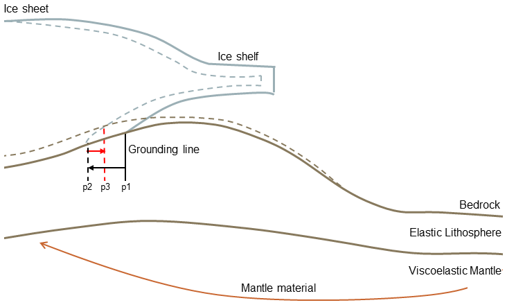
Figure 1 Schematic figure of GIA feedback on the grounding line migration. The solid light gray and brown lines represent the initial ice sheet or ice shelf and bedrock topography, respectively, before the retreat of the grounding line. The solid black line separates the elastic lithosphere and the viscoelastic mantle. Point p1 is the grounding line position corresponding to the initial steady state. The dashed light gray line represents the ice sheet or ice shelf after retreat, the dashed black line is the perturbed mantle elevation, and the dashed brown is the new bedrock surface. Point p2 is the grounding line position after retreat without GIA effects. Point p3 is the grounding line position after the GIA response. The change in sea level is not applied as a load in the GIA model, and only the global mean sea level is prescribed as forcing on the ice sheet model. The sea level is, for this reason, not shown in this figure.

There exist other GIA feedbacks on the ice sheet evolution, apart from the direct effect on the grounding line via the bedrock elevation. First, the local sea level decreases due to the diminishing gravitational attraction of the ice on the surrounding water in case the ice sheet melts (e.g., de Boer et al., 2017; Gomez et al., 2015). As a consequence, a decrease in sea level reduces the load of the ocean on the bedrock and in turn enhances uplift from GIA, although to a smaller degree than the loss of grounded ice. Second, GIA could steepen or flatten the bed slope dependent on the local topography. A flattened bed slope decreases the rate of basal sliding and ice deformation and therefore decreases the ice flux and ice velocity towards the shelves (Adhikari et al., 2014). Finally, GIA stabilizes the ice sheet as it reduces the surface elevation change in the ice sheet caused by surface melt in a warming climate. The reduced lowering of the surface elevation thereby suppresses melt rates (van den Berg et al., 2008).

Several types of models have been developed to include GIA in ice sheet models. A widely used approach to take changes in bedrock topography into account is by using an Elastic Lithosphere Relaxed Asthenosphere model (ELRA; Le Meur and Huybrechts, 1996). This is a two-layer model that contains a local elastic layer and an asthenosphere that relaxes with a single constant relaxation time. This simplified model is computationally cheap and provides a first-order estimate of bedrock changes (e.g., Pelletier et al., 2022; de Boer et al., 2017; Pattyn, 2017). However, the ELRA approach assumes a radially and laterally homogeneous flat Earth, while the actual Earth properties vary spatially. To partly overcome these limitations, Coulon et al. (2021) included regions with different relaxation times in the ELRA model to capture the main patterns of the spatial variability in the relaxation timescale. Still, ELRA neglects the effect of self-gravitation, the size dependency of the Earth's response to ice loading, and the fact that larger ice sheets respond to deeper Earth characteristics and smaller ice sheets respond to shallower Earth characteristics (Wu and Peltier, 1982).

The solid Earth response is mainly determined by the thickness of the elastic lithosphere and the viscosity of the mantle. ELRA models have been improved by coupling the lithosphere with a viscous half-space, where the mantle viscosity can be used as an input parameter instead of the relaxation time (Albrecht et al., 2020; Bueler et al., 2007). Another approach for computing GIA is self-gravitating viscoelastic (SGVE) spherical Earth models. They compute the response to global ice sheet thickness changes with radially varying Earth models, labeled 1D GIA models, that account for gravity field perturbations. Most 1D GIA studies also account for the relative sea level change by solving the sea level equation (DeConto et al., 2021; Pollard et al., 2017; Konrad et al., 2015; de Boer et al., 2014; Nield et al., 2014; Gomez et al., 2013; Whitehouse et al., 2012). For Antarctica, these 1D GIA models commonly use an Earth structure with a strong upper-mantle viscosity of 10²⁰–10²¹ Pa s and a lithosphere of ∼100 km thick, which is close to the Antarctic average (Gomez et al., 2018; Geruo et al., 2013). The present-day ice surface elevation resulting from a coupled 1D GIA–ice sheet model with a mantle viscosity of 10²¹ Pa s can be achieved with reasonable accuracy by the ELRA approach with a relaxation time of 3000 years, but the deformation through time differs, and it is not known how well other viscosities can be approximated (Pollard et al., 2017; van den Berg et al., 2008; Le Meur and Huybrechts, 1996).

However, even 1D GIA models are oversimplified for realistic Antarctic conditions. It can be derived from seismic data that the viscosity of the mantle under the AIS varies laterally with 6 orders of magnitude, with much lower viscosities ∼10¹⁸ Pa s in West Antarctica than the generally assumed global average mantle viscosity (Hay et al., 2017; van der Wal et al., 2015; Ivins et al., 2021). In these low-viscosity regions, the Earth's mantle approaches isostatic equilibrium 1 to 2 orders of magnitude faster than the timescale of 3000 years that is commonly used in the application of ELRA models (Whitehouse et al., 2019; Barletta et al., 2018). This can only be overcome by 3D GIA models which have been developed to simulate GIA using a lateral variable rheology in Antarctica (Yousefi et al., 2022; Blank et al., 2021; Powell et al., 2021; Nield et al., 2018; Hay et al., 2017; van der Wal et al., 2015; Geruo et al., 2013; Kaufmann et al., 2005), but those approaches have so far neglected the GIA feedback on the ice sheet evolution because they use a predefined ice sheet history.

Whitehouse (2018) emphasize the importance of coupled 3D GIA–ice sheet models for studying regions with a low mantle viscosity, and there are ongoing efforts to develop an efficient coupling method with a high temporal resolution using a 1D GIA model (Han et al., 2021). Coupled GIA–ice sheet models need an iterative method to include the GIA feedback, since ice sheet models need bedrock deformation as input to compute the ice thickness, and GIA models need ice thickness as input. We define a coupling time step as the time period over which the ice sheet model and GIA model exchange ice thickness and bedrock elevation during a fully coupled transient experiment. There are coupled 1D GIA–ice sheet models that use short coupling time steps of tens of years, but those models simulate projections and hence consider a much shorter timescale than the glacial cycle (DeConto et al., 2021; Konrad et al., 2015). The only model that couples 3D GIA with ice dynamics is developed by Gomez et al. (2018), who show significant differences in ice thickness of up to 1 km in the Antarctic Peninsula and the Ross Embayment when a 3D Earth rheology was used instead of a 1D rheology. From this model, it can be concluded that uplift is typically underestimated in West Antarctica and overestimated in East Antarctica when using lateral homogenous Earth structures in ELRA or 1D GIA models (Nield et al., 2018). Gomez et al. (2018) apply the following iteration method to simulate the AIS evolution from 40 ka to the present day. First, the 3D GIA model computes bedrock elevation changes relative to the geoid at time steps of 200 years for the entire 40 kyr, using ice thickness changes from a previous coupled 1D GIA simulation. These bedrock elevation changes are corrected at each time step for the difference between the simulated present-day bedrock topography and the observed present-day topography. The corrected bedrock elevation changes are passed to the ice sheet model to recompute the ice thickness history for the entire period of 40 kyr till the present day, with time steps of 200 years. Finally, the new ice thickness history is passed to the 3D GIA model, and the process is repeated until the ice and bedrock elevation histories converge. Typically, only four iterations are needed. However, both models are still simulated over the entire period of 40 kyr, with a fixed ice or bedrock elevation history as input. As a consequence, the coupling time step between ice sheet model and 3D GIA model is 40 kyr. Yet, for example, in the Amundsen Sea embayment in West Antarctica, GIA occurs on decadal to centennial timescales (Barletta et al., 2018). Present-day GIA estimations and the evolution of the ice sheet could therefore be improved by including the 3D GIA feedback in a coupled model at coupling time steps shorter than 40 kyr.

This study presents a method to fully couple an ice sheet model and a 3D GIA model on century to millennial timescales from 120 ka onwards. The method simulates the 3D GIA feedback by iterating an ice sheet model and a 3D GIA model at every single coupling time step. The method is applied using the ice sheet model ANICE (de Boer et al., 2013), and a 3D GIA finite element (FE) model (Blank et al., 2021), where the coupling time steps are 5000 years over the glaciation phase and vary between 500 and 1000 years over the deglaciation phase of the last glacial cycle. The GIA model computes deformation due to ice loading and does not solve the sea level equation, but the viscoelastic model does account for the effect of the self-gravitation of the mantle deformation when a 1D Earth structure is used. To decrease computational time, the GIA model excludes the effect of self-gravitation when a 3D Earth structure is used, which is explained in Sect. 2.2. Global mean sea level (GMSL) from the Northern Hemisphere ice sheets is prescribed in the ice sheet model. The ice sheet model is applied to Antarctica to assess the impact of the stabilizing GIA effect on the AIS evolution over the last glacial cycle using 1D and 3D Earth structures.

We assess whether widely used 1D Earth structures, for example, those used by Pollard et al. (2017), yield similar stability characteristics for ice sheet evolution caused by bedrock uplift in comparison to 3D Earth structures during the deglaciation phase. The developed coupled model can be applied to different regions, and the coupling method could be applied to different ice sheet models and GIA models. The model has the potential to improve GIA estimates and hence corrections for ongoing GIA to geodetic data (e.g., Scheinert et al., 2021; The IMBIE team, 2018). This method can not only be applied to improve glacial–interglacial ice sheet histories but also for projections of the AIS evolution.

2 Method

The coupling method that we present in this paper can be applied to any ice sheet and GIA model, as long as the models have the possibility to restart at certain time steps. We applied the coupling method to the ice sheet model ANICE and the 3D GIA model, which are introduced first in Sect. 2.1 and 2.2. The coupling method alternates between the ice sheet model and the GIA model, where the ice sheet model uses the bedrock deformation computed by the GIA model and the GIA model uses the changes in ice thickness computed by the ice sheet model. The interpolations that are necessary to feed the ice sheet model output to the GIA model and the GIA model output to the ice sheet model are performed using Oblimap (Reerink et al., 2016) and discussed in the Supplement (see p. 5). Finally, we describe the coupling method in Sect. 2.3. The models are coupled at a coupling time step that varies during a glacial cycle. During the glaciation phase, the coupling time step is 5000 years, and during the deglaciation phase, the coupling time step is 1000 and 500 years. The effect of the size of the coupling time step is discussed in Sect. 2.3.1. At intermediate time steps, the ice sheet model uses a linear interpolation of the bedrock changes, and the GIA model uses a linear interpolation of the ice thickness changes.

2.1 Ice sheet model: ANICE

The ice sheet model ANICE is a global 3D ice sheet model allowing us to simulate the AIS, Greenland ice sheet, Eurasian ice sheet, and North American ice sheet separately or simultaneously (de Boer et al., 2013). Each ice sheet can be simulated on different equidistant grids. The horizontal resolution is 20 km for Greenland and 40 km for the other regions. The temporal resolution of ANICE is 1 year (hereafter referred to as the ANICE time step). ANICE has been used for a variety of experiments (Berends et al., 2019, 2018; Bradley et al., 2018; de Boer et al., 2017, 2013; Maris et al., 2014). For this study, ANICE is used to simulate the Antarctic ice sheet evolution with a resolution of 40 km×40 km. Atmospheric temperature and GMSL act as the main forcing for the ice sheet model, as shown in Fig. S1 in the Supplement, and are the result of previous ice volume reconstructions using ANICE and benthic isotope forcing (de Boer et al., 2013). The accumulation for the ice sheet is computed using present-day monthly precipitation from ERA40, which are temporally extrapolated as a function of the free-atmospheric temperature (Bintanja et al., 2005; Bintanja and van de Wal, 2008). A time- and latitude-dependent surface temperature–albedo–insolation parameterization is used to calculate ablation (Berends et al., 2018). Insolation changes are based on the solution by Laskar et al. (2004). The shallow-shelf approximation (SSA; Bueler and Brown, 2009) is used to solve mechanical equations to determine the sliding and velocities of ice shelves, and the shallow-ice approximation (SIA) is used to compute the velocities of grounded ice (Morland, 1987; Morland and Johnson, 1980). Basal sliding follows a Weertman friction law, where friction is controlled by bed elevation. The position of the grounding line and GMSL determine whether ice is grounded or floating and thus whether the ice experiences subshelf melt or not. A combination of the glacial–interglacial parameterization by Pollard and DeConto (2009) to scale the global mean ocean temperature beneath the shelf and the ocean temperature-based formulation by Martin et al. (2011) are used to compute subshelf melt. This parameterization assumes a linear relation between subshelf melt and ocean temperature. Changes in ocean circulation are not taken into account.

Besides the effect of GMSL, there is an effect from regional sea level variations as well. Although the effect of the Northern Hemisphere ice sheets on GMSL is significant, the effect of the AIS itself is most important for regional sea level (Gomez et al., 2020). At regions where grounded ice melts, such as the Ross and the Filchner–Ronne embayments during the deglaciation phase, the near-field sea level is reduced due to the decreasing gravitational attraction between the ice sheet and the ocean. De Boer et al. (2014) studied the differences between using ANICE with a gravitationally self-consistent sea level and with a global mean sea level. At the last glacial maximum, the ice volume of the AIS is lower when including the regional sea level because the increased regional sea level due to the increased gravitational attraction of the growing ice sheet leads to a small reduction in the grounded ice. During the deglaciation, the differences in ice volume are small. The spatial variation caused by the Northern Hemisphere ice volume changes over a glacial cycle is smaller than the spatial variation in the regional sea level by Antarctic changes and is therefore considered a second-order effect. The regional sea level variation is not yet included in this model.

The standard version of ANICE uses the ELRA method to compute the bedrock elevation changes using a uniform relaxation time that is usually taken to be 3000 years. For this study, ANICE is adjusted to use the bedrock deformation computed by a GIA model instead of computing the bedrock deformation using the ELRA method (see Sect. 2.3.1 for an explanation of the chosen coupling time steps). The initial topography at 120 ka is taken from ALBMAP (Le Brocq et al., 2010). Within one coupling time step, the bedrock elevation is updated in ANICE at time steps of 1 year, using the linear interpolation of the deformation computed by the GIA model as follows:

$$\begin{array}{}\text{(1)}& b_t=b_{t\mathrm{0}}+{\displaystyle \frac{\mathrm{\Delta }b}{\mathrm{\Delta }{t}_{\text{coupling}}}}\cdot \mathrm{\Delta }{t}_{\text{ANICE}},\end{array}$$

where b_t refers to the updated bedrock elevation at the ANICE time step; b_t0 refers to the bedrock elevation at the beginning of the coupling time step; $\frac{\mathrm{\Delta }b}{\mathrm{\Delta }{t}_{\text{coupling}}}$ refers to the total deformation of one coupling time step computed by the GIA model divided by the length of the coupling time step in years; and Δt_ANICE refers to the ANICE time step of 1 year. Linear interpolation introduces the inaccuracy of the true GIA deformation, which generally follows an exponential curve. As a consequence, the total deformation at the end of the coupling time step is the same, but the deformation would be slightly underestimated at the beginning of the coupling time step. This effect is higher at regions with a lower viscosity of the Earth's mantle due to the increased nonlinearity of the Earth's response when compared to higher-viscosity regions. The effect of this approximation can be reduced by reducing the length of the coupling time step, as shown in Sect. 2.3.1.

2.2 GIA model

The GIA finite element (FE) model from Blank et al. (2021) is used, which is based on the commercial finite element method (FEM) software Abaqus, following Wu (2004). It computes bedrock changes for surface loading on a compressible spherical Earth (υ=0.28), with a composite and Maxwell rheology. The effect of density variations required for full compressibility is not included. Each element of the model is assigned a dislocation and diffusion parameter from which the mantle viscosity can be computed based on, among others, the applied stress from surface loading. Section 2.2.2 discusses how these parameters and the viscosity are computed. The FEM approach allows for the discretization and computation of stresses and the resulting deformation in the Earth, using a modified stiffness equation and Laplace's equation (Wu, 2004). The ice loading is applied to the GIA FE model at each coupling time step. When running the GIA FE model, each coupling time step is divided in increments for numerical integration inside the finite element model. The size of each subsequent increment is determined based on how fast the computation of the deformation converges. In this study, each coupling time step is divided into approximately 30 increments so that the nonlinear solution path can be followed with sufficient accuracy. The advantage of this FEM approach, which is based on Abaqus, is its flexibility, as its grid size and rheology can be adjusted. Furthermore, FE models operate in the time domain, so the program can be stopped at each time step, and all information about the state of stress is stored. This is contrary to SGVE models that operate in the Laplace domain for which the entire ice history has to be available to compute the next time step (e.g., de Boer et al., 2014), thus introducing complications if the coupled evolution is addressed. Because of the solution in the temporal domain, FE models can exchange information with the ice sheet model at every required time step. This advantage allows, for example, the simulation of the glaciation phase of the last glacial cycle at once on a high spatial and temporal resolution and the use of the state of the Earth at the end of the glaciation phase as a starting point for different experiments of the deglaciation phase, where, for example, the coupling step size or the forcing of the ice sheet model is adjusted. The restart option also allows the simulation of projections where the model is restarted from an initialized GIA FE–ice sheet model.

The adopted 3D GIA FE model from Blank et al. (2021) used a prescribed ice load history for all time steps in the GIA FE model and iterates several times over the past 120 000 years to include self-gravitation (Wu, 2004). However, restarting with a different ice load at each coupling time step is necessary to include the GIA feedback on the ice dynamics. For this reason, adjustments to the GIA FE model have been made in order to continue the GIA FE model with a new ice load after each coupling time step using the restart option in Abaqus. When simulating the 1D Earth structures, two iterations of the GIA FE model are performed over each coupling time step to include self-gravitation before moving on to the next time step. When simulating the 3D Earth structures, only one iteration of the GIA FE model is performed over each coupling time step to decrease the simulation time by 50 %. The difference between including and excluding the effect of self-gravitation is less than 10 % of the total deformation, as shown in Fig. S2 in the Supplement. For future studies, the same iteration over each coupling time step could be used to solve the sea level equation (Wu, 2004; Blank et al., 2021) and rotational feedback (Weerdesteijn et al., 2019).

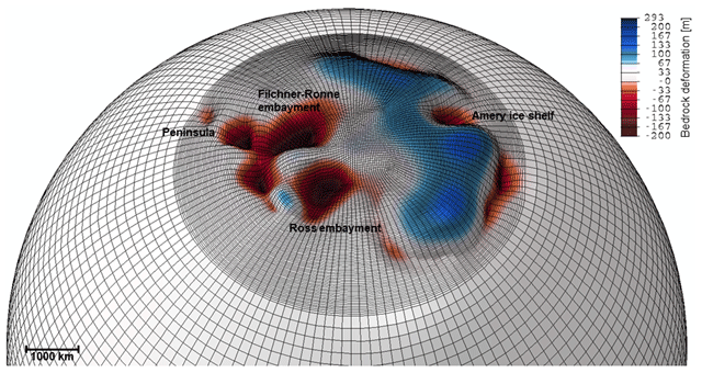
Figure 2 An example of the deformed Earth simulated by the GIA FE model at 115 ka. The grid has a higher-resolution area of 30 km by 30 km at latitudes until −60^∘ and a lower-resolution area of 200 km by 200 km above −60^∘ latitude. The ice sheet is mainly growing in West Antarctica, causing subsidence, and slightly decreasing in East Antarctica, which causes uplift.

The applied changes in ice loading are relative to the present-day ice load, as it is assumed that the Earth was in isostatic equilibrium with present-day ice loading at the beginning of the last glacial cycle. The ice load is computed at each time step by computing the grounded-ice thickness above floatation, taking into account the relative sea level change, as described in Simon et al. (2010). The ice load is computed by ANICE using

$$\begin{array}{}\text{(2)}& H_{\text{AF}}=H-max\left(\mathrm{0},(\text{SL}-b)\cdot {\displaystyle \frac{{\mathit{\rho }}_{\mathrm{w}}}{{\mathit{\rho }}_{\mathrm{i}}}}\right),\end{array}$$

where H_AF refers to the ice thickness above floatation of grounded ice; H refers to the ice thickness of grounded ice; SL refers to the sea level relative to present-day sea level; b refers to the bedrock elevation relative to present-day sea level; and ρ_w and ρ_i refer to the density of water and ice, respectively. The change in ice load is applied as a linear change on the GIA FE model during each coupling time step. This is an approximation of the true ice dynamics over the coupling time step, of which the ice dynamic equations are solved on much shorter timescales (1 year) than the coupling time steps and are nonlinear. The determination of the chosen coupling time steps of 5000, 1000, and 500 years is described in Sect. 2.3.1.

Not only ice loading but also loading ocean cause deformation due to temporal variations in sea level. We conducted a test in which we prescribed a spatially variable global ice and ocean loading caused by other ice mass changes, taken from Whitehouse et al. (2012), in addition to loading from the Antarctic ice sheet model. From the results of the test, we conclude that the effect of global ocean and ice loading on deformation could be important on the scale of individual glaciers in Antarctica, but the load of global ice and ocean loading from other ice mass changes was negligible when compared to the ice load variations on the scale of the AIS. Including global loading in the GIA FE model increases the computation time because a load is applied to every surface element globally instead of only on the surface elements for which there is a change in grounded ice in Antarctica. Thus, loading due to other ice masses, spatially variable ocean loading, and loading due to variations in Earth's rotation are not considered with the aim of reducing the computational burden, as this paper focuses on the direct effect of mantle viscosity.

2.2.1 Model setup and resolution

In the GIA model adopted for this study, referred to as the GIA FE model (Blank et al., 2021; Hu et al., 2017), a different mantle viscosity can be assigned to each element, which allows for the use of 3D Earth structures (van der Wal et al., 2015). Other parameters (such as density and Young's modulus) are deemed constant in layers that represent the core, lower and upper mantle, and the elastic lithosphere. The horizontal grid has a higher resolution over Antarctica, which is visible in Fig. 2. Sensitivity tests for the grid size are conducted for the trade-off of accuracy versus the computation time. For these tests, the GIA FE model is loaded with a parabolic ice cap for 1000 years, using the following four different spatial resolutions, respectively: 70, 55, 30, and 15 km. The details of the test are described in Fig. S3 in the Supplement. The tests show that using a horizontal resolution of 15 km by 15 km instead of 30 km by 30 km decreases the deformation by 0.01 % over 1000 years and increases the computation time of the GIA FE model by approximately 30 % to 15 min (Fig. S3). A coarser resolution of 55 km×55 km does not notably reduce the computation time. Therefore, a resolution of approximately 30 km by 30 km is chosen at the surface in Antarctica from 62^∘ latitude to the South Pole and 200 km by 200 km elsewhere in the GIA FE model. Since the grid lies on a sphere, the elements are not equal, but their size approaches the given resolution. The resolution in the lower mantle and core are double as coarse as the lithosphere and the upper mantle. The chosen resolution results in approximately 300 000 elements being divided over several layers, where the lithosphere and upper mantle have double the elements of the lower mantle and the core. The FE model is divided in eight layers for the 1D simulations and nine layers for the 3D simulations to represent the upper and lower mantle so that the elements in each layer lie at the same depth (see Table 1 for detailed parameters of the layers). The bottom of the upper mantle is connected to the lower-resolution lower mantle with the use of so-called tie constraints. Figure 2 shows an example of a change in a deformed sphere due to ice unloading at East Antarctica and ice loading at West Antarctica, with a relatively high resolution in and around Antarctica and lower resolution in the far-field.

Table 1 Material properties of the GIA FE model. The top of upper mantle 2 is at 100 km depth for the 1D simulation and at 35 km for the 3D simulation.

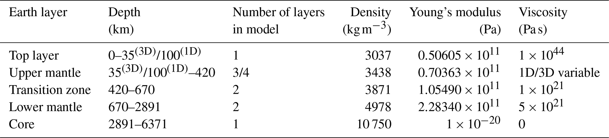
Following the five-layer model used in Spada et al. (2011), one value for density, Young's modulus and, in the case of a 1D model, viscosity is assigned to each layer, as is shown in Table 1. In case of a 3D Earth structure, the elastic top layer is fixed down to 35 km depth, as this is the thinnest lithosphere found in West Antarctica (Pappa et al., 2019), and a 3D rheological model with specific dislocation and diffusion creep parameters is assigned to each element between 35 and 670 km depth, as described in Sect. 2.2.2. The effective lithospheric thickness is therefore spatially variable and follows from the effective mantle viscosity. If the viscosity in a region is so high that viscous deformation in one of the top layers is negligible over the entire cycle, then the region can be considered to be part of the lithosphere (e.g., van der Wal et al., 2013; Nield et al., 2018). This will lead to a thicker effective lithosphere than 35 km in most of Antarctica. Thus, the second model layer consists partly of lithosphere and partly of upper mantle and is called the shallow upper mantle in Table 1. In the 1D model, the lithosphere is prescribed as being 100 km thick, which is similar to the lithospheric thickness used in Gomez et al. (2018). The chosen viscosities of 5×10²¹ and 10²¹ Pa s for the mantle between 420 and 2891 km depth are shown in Table 1 and are consistent with the GIA-based inferences of radial viscosity (Lau et al., 2016; Lambeck et al., 2014). The core is included in the model only through boundary conditions to provide a buoyancy force on the mantle (Wu, 2004). The complete overview of the parameter setup is shown in Table 1.

2.2.2 Rheology and seismic models

The deformation as a result of the applied ice load depends on the rheological model that is used by the GIA FE model. Rheological models describe the relation between stress and strain. The 1D version of the GIA FE model uses a linear Maxwell rheology at all depths, whereas the 3D version uses a composite rheology, following van der Wal et al. (2010), at depths between 30 and 420 km (see Table 1). The composite rheology combines two deformation mechanisms, diffusion and dislocation creep, such that the strain computed in Abaqus is

$$\begin{array}{}\text{(3)}& \mathrm{\Delta }{\mathit{ϵ}}_{ij}={\displaystyle \frac{\mathrm{3}}{\mathrm{2}}}(B_{\text{diff}}+B_{\text{disl}}{\stackrel{\mathrm{̃}}{q}}^{n-\mathrm{1}})q_{ij}\mathrm{\Delta }t,\end{array}$$

where Δϵ_ij is the strain; B_diff and B_disl are the spatially variable diffusion and dislocation parameters, respectively; $\stackrel{\mathrm{̃}}{q}$ is the von Mises stress, which is assumed to be 0.1 MPa (Ivins et al., 2021); n is the stress exponent, which is taken to be 3.5, consistent with Hirth and Kohlstedt (2003); q_ij is the deviatoric stress tensor; and Δt is a variable time increment for the numerical integration within the coupling time step. The increments are determined automatically, depending on the applied stress and the size of the coupling time step. A detailed explanation of the implementation of the composite rheology in the FE model can be found in Blank et al. (2021).

From Eq. (3), it can be derived that the effective viscosity (η_eff) for each element of the GIA FE model (van der Wal et al., 2013) becomes

$$\begin{array}{}\text{(4)}& {\mathit{\eta }}_{\text{eff}}={\displaystyle \frac{\mathrm{1}}{\mathrm{3}{B}_{\text{diff}}+\mathrm{3}{B}_{\text{disl}}{q}^{n-\mathrm{1}}}}.\end{array}$$

The diffusion and dislocation parameters used in this study are derived from the flow law from Hirth and Kohlstedt (2003) and are given by Eq. (5a) and (5b), respectively.

$$\begin{array}{}\text{(5a)}& {\displaystyle }{B}_{\text{diff}}=A_{\text{diff}}{d}^{-\mathrm{3}}{f}_{{\mathrm{H}}_{\mathrm{2}}\mathrm{O}}^{\mathrm{1}}{e}^{-\frac{E+PV}{R{T}_{x,y}}},\text{(5b)}& {\displaystyle }{B}_{\text{disl}}=A_{\text{disl}}{d}^{\mathrm{0}}{f}_{{\mathrm{H}}_{\mathrm{2}}\mathrm{O}}^{\mathrm{1.2}}{e}^{-\frac{E+PV}{R{T}_{x,y}}},\end{array}$$

where A is experimentally determined (A_diff=10⁶ MPa; A_disl=90 MPa); d is the grain size; $f_{{\mathrm{H}}_{\mathrm{2}}\mathrm{O}}$ is the water content; E is the activation energy; P is the depth-dependent pressure (Kearey et al., 2009); V is the activation volume; R is the gas constant; and T_x,y is the spatially variable absolute temperature. A, E, and V are different, according to the values for wet and dry olivine. All parameters, except temperature, grain size, and water content, are taken from Hirth and Kohlstedt (2003). The temperature is derived from an Antarctic seismic model and a global seismic model for each element of the GIA FE model, following approach 3 in Ivins et al. (2021). Following this approach, seismic velocity anomalies are converted to temperature, assuming that all seismic velocity anomalies are caused by temperature variations (Goes et al., 2000). Derivatives of seismic velocity anomalies to temperature anomalies are provided as a function of depth in the mantle (Karato et al., 2008). Antarctic seismic velocity anomalies are taken from Lloyd et al. (2020) and global velocity anomalies for regions above −60^∘ latitude are taken from SMEAN2, which is an average of three seismic models (Becker and Boschi, 2002). The models are combined with a smoothing applied at the boundary at −60^∘ latitude. Mantle melt is assumed to have a relatively small influence on the upper-mantle viscosity and is therefore not included in this study (van der Wal et al., 2015).

Following Eqs. (3)–(5), the mantle viscosity, and thus the deformation, is dependent on the grain size and water content. As little information about grain size and water content exists, these parameters are kept spatially homogeneous (van der Wal et al., 2015). We obtained two different 3D rheologies by choosing a grain size of 4 mm and a water content of 0 ppm (parts per million; hereafter referred to as 3Ddry) and 500 ppm (hereafter referred to as 3Dwet) to obtain rheologies that can be considered realistic based on other viscosity studies (e.g., Blank et al., 2021; Gomez et al., 2018; Hay et al., 2017). A water content of 500 ppm is within the range of water content found in Antarctic xenoliths (Martin, 2021).

The two rheology models give an idea of some, though not all, of the variation in 3D mantle viscosity. The viscosity of both 3D rheologies is shown at three depths in the two right columns of Fig. 3 (Fig. 3c and d, g and h, and k and l). Increasing the water content lowers the mantle viscosity, but the pattern of the viscosity variations is maintained (Karato et al., 1986; Blank et al., 2021). This can be seen in Fig. 3, where the mantle viscosity of 3Ddry is approximately 1 order of magnitude higher than the mantle viscosity of 3Dwet. Both 3D rheologies provide an upper-mantle viscosity of approximately 10¹⁸ Pa s in West Antarctica, which is comparable with Barletta et al. (2018), who estimated such low viscosities in West Antarctica by constraining the GIA model using GPS and seismic measurements, and with Blank et al. (2021), who confirmed that a mantle viscosity of 10¹⁸⁻¹⁹ Pa s is plausible in the Amundsen Sea sector, based on the WINTERC 3.2 temperature model, which is constrained by seismic data and satellite gravity data (Fullea et al., 2021). The viscosity pattern of both 3D rheologies used in this study and the viscosity value of the 3Ddry rheology are similar to the mantle viscosity used by Gomez et al. (2018) and Hay et al. (2017), who infer mantle viscosity by scaling seismic anomalies to viscosity anomalies and adding them to the background viscosity profile from GIA or geodynamic studies. A background viscosity can be inferred from other GIA or geodynamic studies; however, following the method from van der Wal et al. (2015) allows us to directly obtain absolute viscosity values from seismic measurements without the need to assume a background viscosity profile.

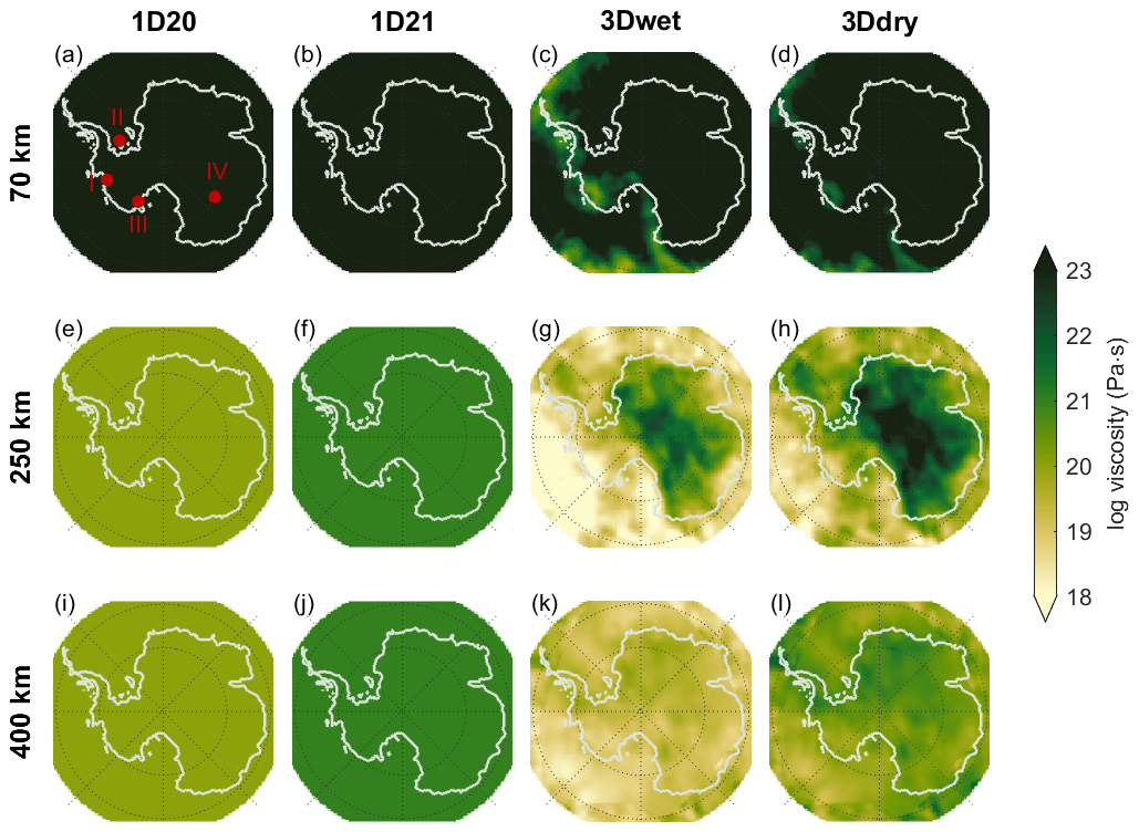
Figure 3 Panels (a), (e), and (i) correspond to the 1D rheology referred to as 1D20. The red dots annotated by roman numbers in panel (e) correspond to the viscosity profiles shown in Fig. S4. Panels (b), (f), and (j) correspond to the 1D rheology referred to as 1D21. Panels (a) and (b) show a viscosity of 10⁴⁴ Pa s, representing the 100 km thick lithosphere in the 1D rheology. Panels (c), (g), and (k) correspond to a 3D rheology, with a water content of 500 ppm, referred to as 3D (wet). Panels (d), (h), and (l) correspond to a 3D rheology, without water content, referred to as 3D (dry). Both 3D rheologies assume a grain size of 4 mm. A pressure of 0.1 MPa is used to compute the viscosity from the dislocation and diffusion parameters.

The results of the coupled model using a 3D rheology can be compared with the results using 1D rheologies. Two experiments are performed using a 1D rheology with two different upper-mantle viscosity profiles, namely 10²⁰ Pa s (hereafter referred to as 1D20) and 10²¹ Pa s (hereafter referred to as 1D21). These values are consistent with the lower and upper boundaries of the upper-mantle viscosity that is generally used in studies for Antarctica (e.g., Albrecht et al., 2020; Pollard et al., 2017; Gomez et al., 2018). The elastic lithospheric thickness is the same for both 1D experiments and is set to 100 km. Figure S4 in the Supplement shows the viscosity profile at four different locations for the four different rheologies. The locations are indicated by the numbers in Fig. 3a. At the Thwaites Glacier (location I in Fig. 3a), the viscosity of the 3D rheologies is between 10²⁰ and 10²² Pa s at between 70 and 100 km depth, whereas the 1D rheologies assume this layer to be elastic. On the other hand, at Dome C (location IV in Fig. 3a), the viscosity is above 10²³ at between 100 and 170 km depth for the 3D rheologies, whereas the 1D rheologies assume a viscosity of 10²¹ and 10²⁰ Pa s at between 100 and 170 km depth. In general, the viscosity of the 3D rheologies are up to 4 orders of magnitude lower in West Antarctica and up to 3 orders of magnitude higher in East Antarctica compared to the 1D21 rheology. It should be noted that the response of the bedrock to changes in ice loading does not solely depend on the local viscosity but also on the viscosity of the whole region where the change in ice load occurs.

2.3 Iterative coupling method

The simulation of ice dynamics for a certain coupling time step requires the deformation of the Earth over the coupling time step. On the other hand, the computation of the deformation over this coupling time step, using the GIA FE model, requires the change in ice mass over that coupling time step. For this study, an iterative coupling scheme has been developed that alternates between the models per time step with a varying length of 500 to 5000 years. The GIA and ice sheet model outputs (bedrock deformation and change in ice thickness, respectively) are generated on different grids, and the corresponding interpolation method is described in the Supplement. The iterative scheme is shown in Fig. 4. The ice thickness and deformation at each coupling time step of the coupled model is computed as follows:

1. Simulate the evolution of the AIS for the first coupling time step using ELRA. Then use the difference in the grounded-ice thickness at the end of the coupling time step and the initial grounded-ice thickness as input for the GIA FE model, which starts initially in isostatic equilibrium.

2. Run the GIA FE model to compute the deformation of the Earth's surface during the first coupling time step. Next, subtract the final bedrock elevation of the coupling time step from the final bedrock elevation of the last time step and interpolate this linearly to obtain deformation at the time steps of the ice sheet model. Then run the ice sheet model to compute the new ice sheet evolution at the first coupling time step using the updated deformation in the linear increases during the coupling time step. The ice sheet model and the GIA FE model use their own internal time stepping, as discussed in Sect. 2.1 and 2.2, respectively.

3. Continue the iterative process described in step 2 until a convergence criterion has been reached. The convergence of the coupled model and the required number of iterations is further described in Sect. 2.3.2.

4. Take the average deformation of the last two iterations as the final deformation to minimize the uncertainties in areas where the coupled model does not converge to zero but alternates between positive and negative values. Then pass the average deformation to the ice sheet model and run the model to calculate the final ice sheet evolution over the first coupling time step.

5. Save all stresses present at the end of the first coupling time step in the GIA FE model, which will be restarted in the second coupling time step. The final configuration of the ice sheet model at the end of the first coupling time step is also saved and used as a starting point for the ice sheet model simulation at the second coupling time step. The averaged deformation of the last two iterations of the previous coupling time step will be used as an initial guess to run the ice sheet model for the first iteration of the next coupling time step.

6. Compute the difference between the simulated present-day bedrock topography and the observed present-day bedrock topography using Eq. (6) once the simulation over the entire glacial cycle has finished, as will be explained further in Sect. 2.3.4. Then repeat the simulation of the entire glacial cycle using a corrected initial topography. Repeat the glacial cycle two to four times to convergence to a simulated present-day topography equal to the observed present-day topography.

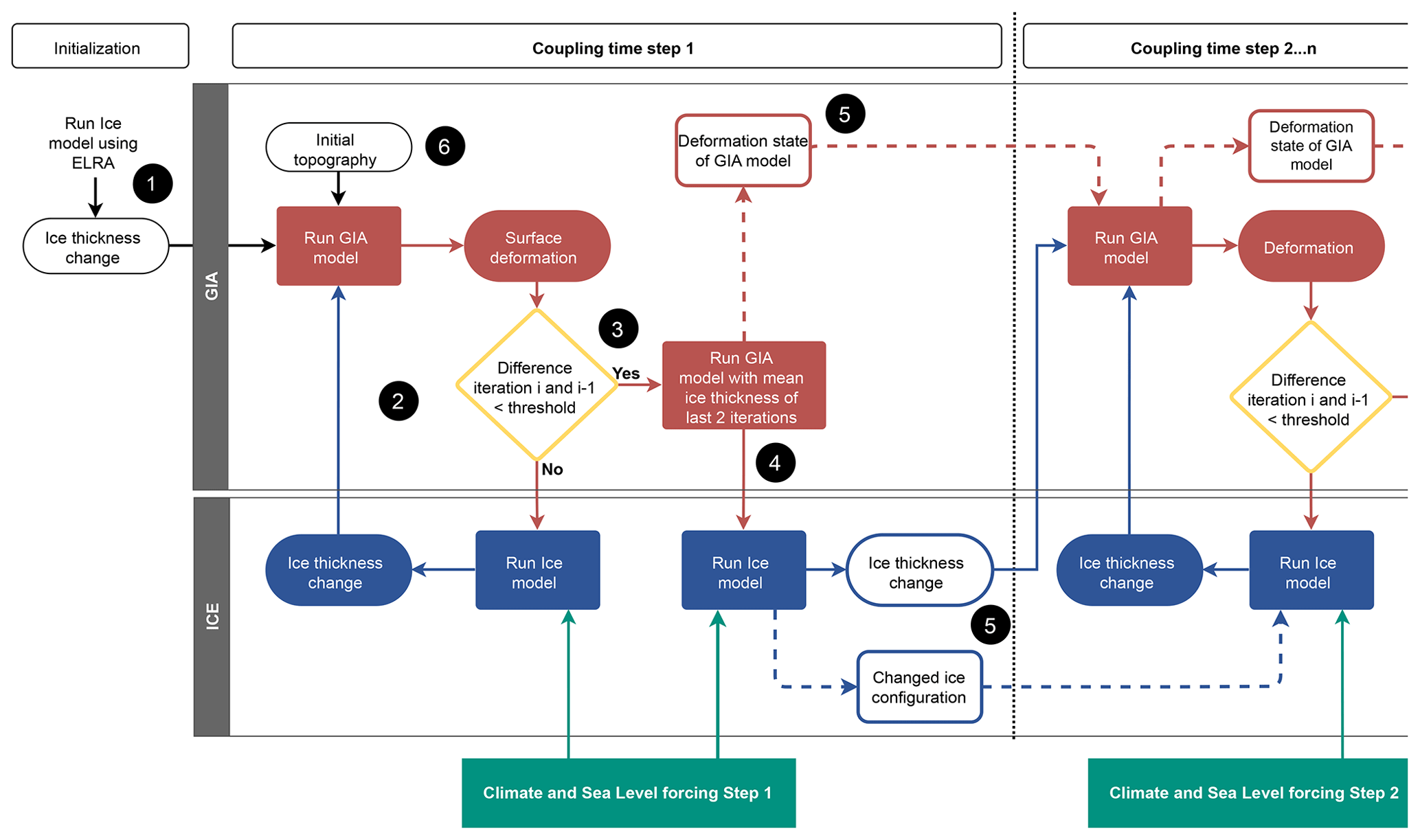
Figure 4 Schematic overview of the method for coupling the GIA and ice sheet model. The numbers 1 to 6 in black circles refer to the steps of the iterative coupling process explained in the main text. The solid lines refer to the flow of the input and output. The dashed lines connect the blocks for running the GIA or ice model to show that the saved model of the previous coupling time step is used to restart the model in the next coupling time step.

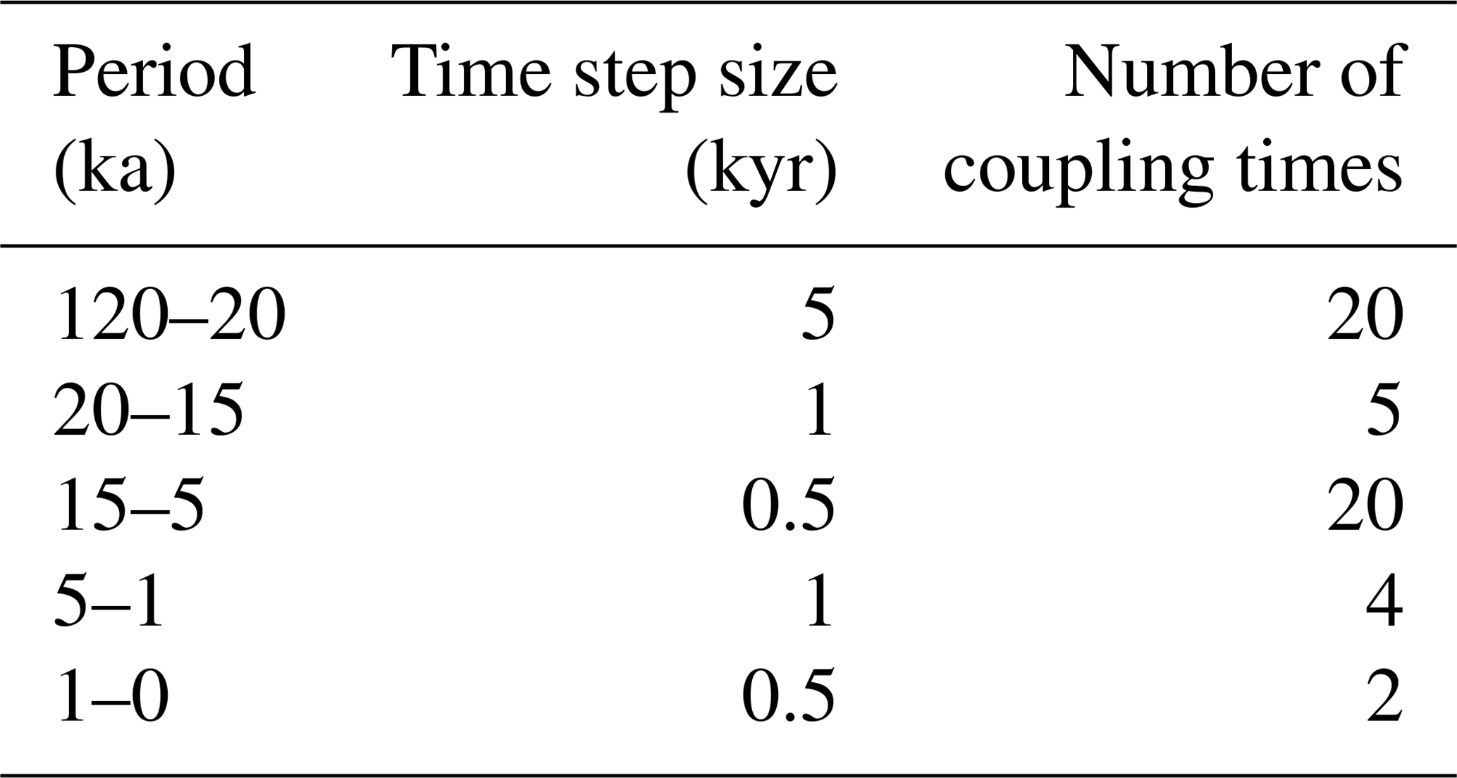
Gomez et al. (2018) create ice loading and bedrock deformation histories of 40 kyr, with a temporal resolution of 200 years, and run the ice sheet model and sea level model alternately at once over the full history. In the method used in this study, the ice sheet model and GIA FE model run alternately at each dynamic coupling time step so that the coupling time step can be changed, depending on the desired accuracy. However, the GIA FE model used in this study does not solve the sea level equation, which should be included in the GIA FE model for realistic reconstructions. For this study, the last glacial cycle is simulated using 51 coupling time steps of 5000, 1000, and 500 years (Sect. 2.3.1). Tests are performed to determine the required number of iterations per coupling time step (Sect. 2.3.3). After calculating the first glacial cycle, there is usually a mismatch between the modeled and observed topography for the present day. To solve this mismatch, we use two to four glacial cycle iterations, depending on the rheology, each with 51 coupling time steps to correct for the difference in modeled and observed topography (Sect. 2.3.4; e.g., Kendall et al., 2005). The method allows us to use variable coupling time steps throughout the glacial cycle and between iterations of glacial cycles to decrease the total computation time.

2.3.1 Size of the coupling time step

A longer coupling time step increases the deformation and change in ice thickness over one coupling time step. Therefore, the coupling time steps need to be chosen to be sufficiently small, so that the deformation and ice thickness change nearly linearly. On the other hand, a large coupling time step is desirable to limit the computation time. The convergence of the coupled model is highly dependent on the length of the coupling time step, since the change in ice load and thus the bedrock deformation is smaller for smaller time steps, which converge faster.

The coupled model is tested using different coupling time steps for the 1D21 rheology. Relatively long coupling time steps of 5000 and 1000 years are tested between 120 and 20 ka because the change in GIA signal is small within this period, since the ice sheet volume is slowly increasing till the Last Glacial Maximum (LGM), and knowledge of the past climate is limited. Using a step size of 1000 years did not lead to significantly different results compared to using time steps of 5000 years, and we therefore chose a step size of 5000 years for the glaciation phase of the last glacial cycle. Because of the fast reduction in the ice in a warming climate, smaller coupling time steps are required during the deglaciation. Han et al. (2022) showed that coupling time steps of 200 years are optimal for the deglaciation phase in their coupled 1D GIA–ice sheet model. However, their method assumes a constant topography during the coupling time step, which is not the case here, and the topography is updated only at the end of each time step. In our simulation, the topography changes linearly during the coupling time step and is updated every year in the ice sheet model. In addition, we run the ice sheet model twice per coupling time step, whereas in the method of Han et al. (2022), this is done only once per coupling time step. The method of Han et al. (2022) therefore requires smaller coupling time steps between the GIA and ice sheet models than the coupling method presented in this study. To determine the length of the coupling time step of the deglaciation phase, we tested a step size of 200 and 500 years over the period of fast deglaciation between 15 and 5 ka. The results are shown in Fig. S5 in the Supplement, together with Table S1, which shows the exact step sizes used over the glacial cycle. The difference in bedrock elevation between using a step size of 200 and 500 years occurs mainly at the Ross Embayment and the Princess Astrid Coast of Queen Maud Land, and bedrock is maximum of 20 m higher at the present day when a time step of 200 years is used. The ice thickness of the Ross Ice Shelf at present day is 70 m larger when a step size of 200 years is used, and there is no difference in grounding line position. The ice thickness at the Princess Astrid Coast at present day is 680 m larger, and the grounding line lies 80 m further inland when a step size of 200 years is used. However, this region, with its large ice thickness differences, is very small and spans only 120 km. The computation time of simulating a time step of 200 and 500 years is similar, but the 200-year time step requires 42 extra time steps. Using time steps of 200 years between 15 and 5 ka increases the computation time by 56 h. We therefore chose to use time steps of 500 years during the deglaciation phase. We used time steps of 1000 years around the LGM and between 5 and 1 ka to create a smooth transition between the glaciation phase, the deglaciation phase, and the late Holocene. The chosen time steps for the entire glacial cycle for this study are shown in Table 2.

Table 2 Coupling time steps over last glacial cycle.

2.3.2 Convergence of the coupled model

The number of iterations needed to converge is dependent on the change in ice load and the Earth's structure. The coupled model requires 3 to 13 iterations per coupling time step to converge to an incremental change in deformation of less than 3 mm yr⁻¹ in all individual grid cells when using the 1D21 rheology. A different rheology requires a different number of iterations. An example of the convergence of a coupling time step using the 1D21 rheology can be seen in Fig. 5, which shows the difference in deformation and ice thickness between iterations of one coupling time step from 120 till 115 ka. The deformation threshold is set to 3 mm yr⁻¹ for the entire glacial cycle. Figure 5a shows the change in ice thickness, and Fig. 5b shows the change in bedrock elevation over this coupling time step when using the 1D21 rheology. Figure 5c to f show the difference in ice thickness and bedrock elevation compared to the former iteration. The ice thickness and deformation converge for most of Antarctica, except at the Ross Embayment, where the shelf thickness still differs between iteration 2 and 3 due to its high sensitivity to grounding line position.

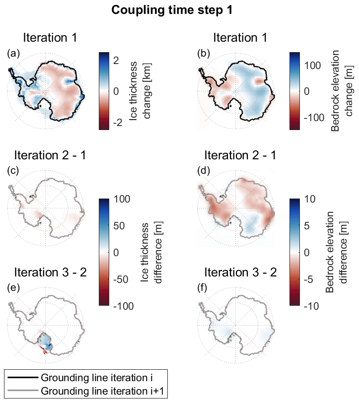
Figure 5 Iterations of coupling time step 1 from 120 to 115 ka, using the 1D21 rheology. (a) Change in ice thickness over this coupling time step. (b) Change in bedrock elevation over this coupling time step. (c–f) Difference in ice thickness and bedrock elevation change compared to the previous iteration. The threshold is set to 10 m over the full coupling time step.

When using the 1D20 rheology, ice thickness and deformation do not converge exactly at multiple locations around the grounding line after iteration 3. A high deformation rate and large changes in ice thickness cause a large shift in the position of the grounding line. Glaciated grid cells of the ice sheet model are defined as grounded ice or floating ice, depending on their position upstream or downstream of the grounding line. If the grounding line in the ice sheet model moves with every iteration due to large changes in deformation, then the grid cells around the grounding line alternate between an ice shelf and grounded-ice status. Since ice thickness can differ by up to hundreds of meters between adjacent grid cells, the difference in ice thickness at one grid cell between iterations can also differ greatly. In this case, both ice thickness and the change in deformation at these grid cells around the grounding line do not converge to zero but to an alternating value. The bedrock deformation converges better than ice thickness because of the stiffness of the Earth causing a smoother deformation pattern.

Tests show that the coupled model converges within an acceptable computation time when the convergence criterion is set to 3 mm yr⁻¹ over the coupling time step. This uncertainty is still below the effect of the uncertainties in the input parameters such as background mantle temperature and seismic velocity (e.g., Blank et al., 2021). Since the grid cells around the grounding line in some cases do not converge to zero, the coupling method introduces an uncertainty. For example, if in one grid cell the change in total deformation over 5000 years keeps alternating between −2 and +2 m, then the uncertainty range is 4 m. To decrease this uncertainty, the average deformation of the last two iterations is used as the final deformation to simulate ANICE for the final iteration of the time step. Decreasing the spatial resolution would allow smoother transitions between grounded and floating ice and thus a further improvement in the convergence. However, the ice sheet model is currently limited to a 40 km resolution.

2.3.3 Number of iterations per coupling time step

Three simulations are conducted to study the effect of the number of iterations on the GIA and the evolution of the AIS using the 1D21 rheology. One simulation is performed with one iteration per time step (which means that the ice sheet model is run twice over the coupling time step, and the GIA FE model is run one time over the coupling time step); one simulation with a varying number of iterations per time step using the convergence threshold, as described in Sect. 2.3.2; and one simulation first simulates the full glacial cycle using the ice sheet model, then a full glacial cycle using the GIA FE model, and finally another glacial cycle using the ice sheet model. Differences in deformation and ice thickness between the three simulations are negligible during the glaciation phase of the last glacial cycle. At the present day, the absolute maximum difference between the convergence simulation and the simulation with only 1 iteration is 700 m in ice thickness at the Ross Embayment, and the grounding line differs by 80 km in this region (Fig. S6 in the Supplement). The maximum difference in ice thickness for the present day is still 2 times smaller than the maximum difference between using different rheology in 1D and 3D and only occurs over very small regions. The absolute maximum difference between the one-iteration simulation and the simulation in which the entire cycle is run at once is much larger, with 3500 m in ice thickness at the Ross Embayment, and the grounding line differs by approximately 800 km in this region (Fig. S7 in the Supplement). From this we conclude that the effect of iterating over the glacial cycle versus iterating per coupling time step is much larger than the effect of the number of iterations over a coupling time step. Furthermore, the effect of decreasing the length of the coupling time step is small.

Reducing the number of iterations significantly reduces the computation time. The coupled model simulations are performed using a 16 CPU Intel^® Xeon^® Gold 6140 CPU at 2.30 GHz, for which the CPU speed varies between 1085 and 2707 MHz. The GIA FE model takes approximately 20 and 40 min to simulate 5000 years for the 1D rheology and the 3D rheology, respectively. The ice sheet model takes only several minutes, so the GIA FE model takes most of the time. A simulation of one glacial cycle using the 1D GIA FE model performing three iterations per coupling time step takes 27 d when running on 16 CPUs performing 51 time steps (which is one glacial cycle). Performing only one iteration reduces the total running time to 30 h. Simulating the last glacial cycle using a 3D GIA FE model takes about 5 d when only 1 iteration per time step is performed, and 37 d when 293 iterations in total are performed.

Considering the long computation time if multiple iterations are used, only one iteration is used for results in the remainder of the paper. This means that for each coupling time step first the ice model is run using the deformation over the former coupling time step, next the GIA FE model is run with the new ice load from the ice model, and, finally, the ice model is run including the new deformation of the GIA FE model.

2.3.4 Iterations over the entire glacial cycle

The bedrock elevation at the last glacial maximum is higher for a larger mantle viscosity, since there is less subsidence during the glaciation phase. In that case, the ice sheet in West Antarctica will melt less, and less bedrock uplift will occur during the deglaciation phase. Thus, the differences in melt during the deglaciation phase for the various rheologies could be caused not only by the direct effect of the viscosity of the rheology on the uplift but also by the difference in bedrock elevation at the last glacial maximum. The direct effect of various rheologies on ice dynamics during the deglaciation phase can be isolated if the model is constrained by ending up at the present day with the observed bedrock topography. Without iterations, the present-day bedrock topography after a glacial cycle differs per simulation and does not equal the observed bedrock topography. For this reason, we apply a commonly used approach in GIA modeling by applying several iterations of the entire last glacial cycle, hereafter called glacial iterations, as described in step 6 of the coupling scheme in Fig. 4. They are needed to ensure that modeled and observed present day bedrock topography are in agreement (Peltier, 1994; Kendall et al., 2005). It is assumed here that this difference is solely caused by modeled vertical GIA deformation, which neglects other types of deformation, such as tectonic motion and erosion or shortcomings in the ice sheet model.

The initial bedrock topography at 120 ka of the first glacial iteration is initially assumed to be equal to the present-day bedrock topography, as taken from ALBMAP (Le Brocq et al., 2010). For the next glacial iterations, the initial bedrock topography is adjusted for the difference in the simulated present-day bedrock topography and the observed present-day topography ALBMAP.

$$\begin{array}{}\text{(6)}& b_{\mathrm{0},i}=b_{\mathrm{0},i-\mathrm{1}}+(b_{\text{ALBMAP}}-b_{\text{PD},i-\mathrm{1}}),\end{array}$$

where the subscript i refers to the iteration over the glacial cycle, b_0,i refers to the bedrock elevation at the beginning of the new glacial iteration, $b_{\mathrm{0},i-\mathrm{1}}$ refers to the bedrock elevation at the beginning of the previous glacial iteration, $b_{\text{PD},i-\mathrm{1}}$ refers to the present-day bedrock elevation of the last glacial iteration, and b_ALBMAP refers to the observed present-day bedrock topography, based on Le Brocq et al. (2010). Four to five iterations of the entire glacial cycle are typically needed to converge the modeled present-day bedrock topography to the observed present-day bedrock topography; the first three iterations are shown in Fig. S8 in the Supplement.

3 Results and discussion

3.1 Testing the coupled model using different 1D rheologies

The evolution of the AIS over the entire last glacial cycle shows a similar ice sheet thickness, extent, and volume when using the 1D coupled model of this study compared to other studies that use coupled 1D GIA–ice sheet models and coupled ELRA–ice sheet models (de Boer et al., 2014, 2017; Gomez et al., 2015; Pollard et al., 2017). To further test if the coupled model works as expected, the results for an upper-mantle viscosity of 10²⁰ Pa s (1D20) are compared to those of 10²¹ Pa s (1D21). The results of both simulations in terms of the ice thickness and grounding line position follow a similar pattern to that in Pollard et al. (2017). The Filchner–Ronne and Ross embayments (indicated with FR and R, respectively, in Fig. 6a) remain larger during the deglaciation phase for the 1D20 simulation than for the 1D21 simulation because the uplift is faster when using the smaller mantle viscosity of 10²⁰ Pa s (Fig. 6). Based on the marine ice sheet instability process, the increased ice shelf melt and fast grounding line retreat can be expected due to a retrograde bedrock slope and an increasing relative sea level caused by subsidence (Schoof, 2007). For the present day, the ice is up to 1 km thinner around the grounding line of the Ross and Filchner–Ronne embayments, and the grounding line has further retreated by approximately 100 km at the Ross Embayment in the 1D21 results compared to the 1D20 results (shown in Fig. 6h).

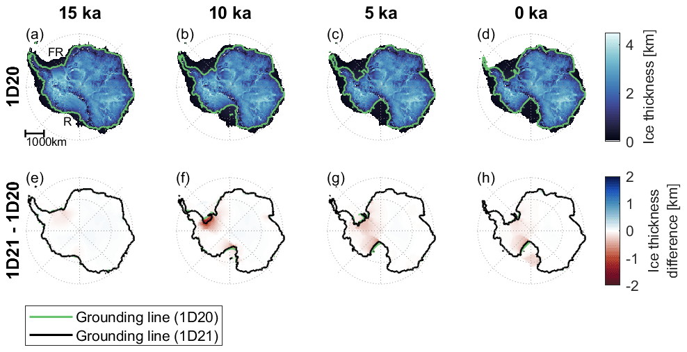
Figure 6 Ice thickness of 1D20 (a–d) and the difference in ice thickness between 1D20 and 1D21 (e–h) at four epochs during the deglaciation phase. (a) FR refers to the Filchner–Ronne Ice Shelf and R refers to the Ross Embayment. In panels (e)–(h), the 1D20 grounding line (green) mostly overlaps with the 1D21 grounding line (black).

3.2 Stabilization of the AIS using 1D and 3D rheologies

In a cooling climate between 120 and 20 ka, all 1D and 3D coupled simulations show an ice thickness increase mainly at the Ross and the Filchner–Ronne embayments and at the peninsula, causing the bedrock to subside in these regions. In the 1D simulations, the bedrock subsides by fewer than 500 m during this period than in the 3Ddry simulations due to the stiffer 1D rheology compared to the 3Ddry rheology (Fig. 7a and d). However, the bedrock subsides by a similar amount when using the 3Dwet rheology compared to the 1D20 rheology during the glaciation phase. At the Amundsen Sea embayment, the mantle viscosity of the 3Dwet rheology is so low that the bedrock responds quickly to slight changes in ice loading. The ice loading follows a fluctuating pattern due to the atmospheric and sea level forcing (Fig. S1), and the bedrock follows the same pattern, although it is dampened and delayed. The bedrock with the 3Dwet rheology subsides over the full glaciation phase but not as much as the bedrock with the 3Ddry rheology because the 3Dwet rheology can respond fast enough to cause uplift in periods when ice thickness does not grow as much.

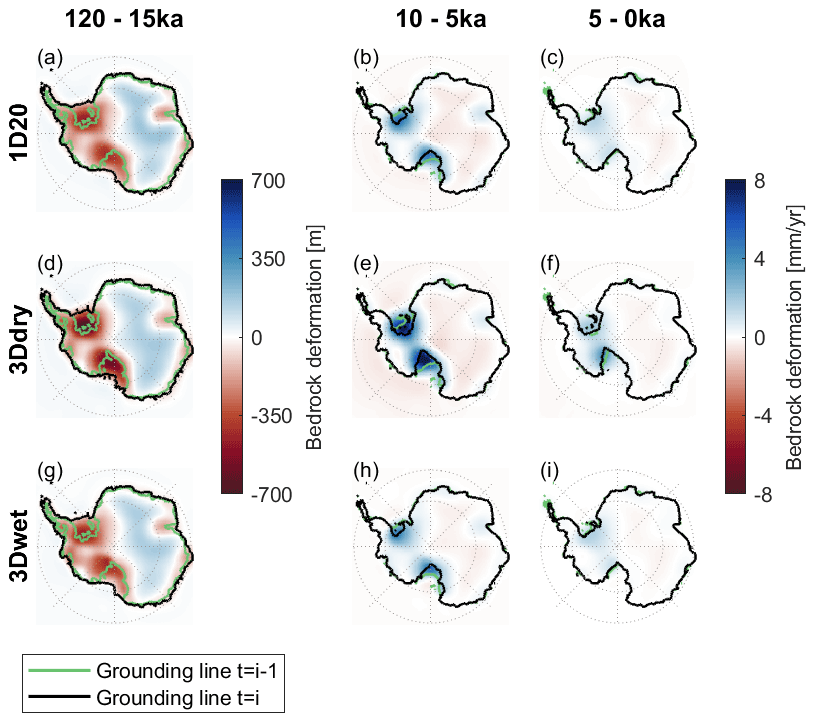
Figure 7 Uplift over the glaciation phase (120–15 ka) for 1D20 (a), 3Ddry (d), and 3Dwet (g). Average uplift rates between 10 ka and the present day for the 1D20 (b, c), 3Ddry (e, f), and 3Dwet (h, i) rheologies. The green grounding line shows the grounding line position at the beginning of the period over which the uplift or uplift rate is computed, and the black grounding line shows the position at the end of the period.

At LGM, the ice thickness is several hundreds of meters larger near the Ross and the Filchner–Ronne embayments when using a 1D rheology compared to the 3Ddry rheology (Fig. 8b and c). During the deglaciation phase, the Ross and Filchner–Ronne embayments retreat fast due to climate warming, similar to what other studies of the AIS evolution suggest (e.g., Albrecht et al., 2020). The 1D mantle viscosity leads to a slower uplift, which causes the grounding line near the Ross and Filchner–Ronne embayments to retreat faster in the 1D simulations than in the 3D simulation (Fig. 7b–c and e–f), corresponding to the results by Pollard et al. (2017) and Gomez et al. (2018). Using a 3Ddry rheology leads to a difference in the grounding line position of up to 700 km and a difference in ice thickness of up to 2 km at the present day along the Siple Coast (Fig. 8c). Using a 3Dwet rheology leads to 600 m thicker ice at the present day compared to using the 1D20 rheology and a more advanced grounding line position of 80 km. The ice thickness of the 3Dwet rheology lies closer to the 1D20 ice thickness than the ice thickness of the 3Ddry rheology because the bedrock elevation at LGM is similar for the 1D20 and the 3Dwet rheologies and is 500 m lower for the 3Ddry rheology. Due to the lower bedrock elevation at LGM when the 3Ddry rheology is used, the ice sheet in West Antarctica will melt more, and faster bedrock uplift will occur during the deglaciation phase when a stronger rheology is used. The differences in melt during the deglaciation phase between using different rheologies is then not caused by the direct effect of different rheologies on uplift rates, but by the difference in the bedrock elevation at the last glacial maximum.

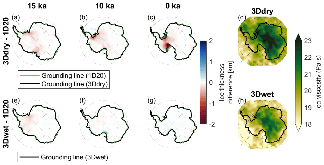
Figure 8 1D vs. 3D ice thickness and mantle viscosity at a depth of 250 km. A stress of 0.1 MPa is used to compute the 3D viscosity from dislocation and diffusion parameters. Here, the 3D grounding lines (black) mostly overlap the 1D grounding line (green).

In contrast to the changes in West Antarctica, Fig. 8 shows that the difference in ice sheet thickness between the 1D and 3Ddry simulations in the interior of the east AIS is not larger than 50 m, although the mantle viscosity in East Antarctica is several orders of magnitude higher in the 3D rheology than in the 1D rheologies. This is because the interior of the ice sheet is not as sensitive to the bedrock elevation as the outlet glaciers near the margin are, leading to an insignificant effect of mantle viscosity differences. The interior of Antarctica is also less sensitive to changes in the surface temperature and sea level and therefore follows an equilibrium response which is independent of the rheology.

As can be seen in Fig. 8, the Antarctic ice mass variability is dominated by the changes in West Antarctica. Figure 9 shows that 1D21 decreases faster than the 1D20 rheology due to the slower uplift in West Antarctica, as shown in Fig. S9 in the Supplement. Figure 9 also shows that the present-day ice volume is 0.2–0.6 km³ lower when using 1D rheologies compared to using the 3Dwet rheology. The use of the 3Dwet rheology stabilizes the ice sheet compared to the use of a 1D mantle viscosity (Fig. 9) because a lower-mantle viscosity at West Antarctica stabilizes the Filchner–Ronne and Ross embayments (Fig. 8). However, the ice volume decreases faster in the deglaciation phase for the 3Ddry rheology compared to the 1D rheologies. That is because the ice volume and ice surface elevation when using the 3Ddry rheology is much lower at LGM than the ice volume when one of the other rheologies is used, and the bedrock uplift during the deglaciation phase is not fast enough to prevent the ice sheet from melting more ice when compared to the other rheologies. The bedrock elevation at the LGM therefore plays a very important role in the determination of the ice sheet evolution during the deglaciation phase.

Gomez et al. (2018) found an insignificant difference in ice volume at the present day for 3D viscosity vs. 1D viscosity. Gomez et al. (2018) included the effect of regional sea level in the coupled model. Including this effect in our model would decrease the ice shelf melt and therefore decrease the ice volume change itself and the difference in ice volume between the 1D and 3D simulations. Differences in terms of ice dynamics formulations, forcings, rheology, and resolution could additionally explain the different results of Gomez et al. (2018) and this study.

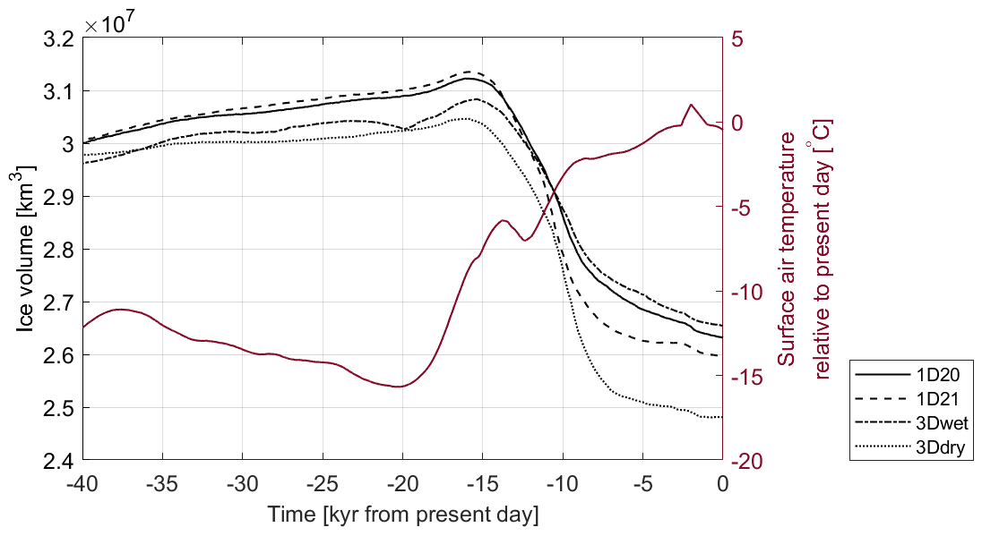
Figure 9 The black lines show the AIS volume over time for the 1D simulations and for the two 3D simulations (dry and wet rheology). The red line shows the mean surface temperature.

Overall, it can be concluded that the variations in the mantle viscosity between a realistic 3D rheology and commonly used 1D rheology have a significant impact on the grounding line position and ice thickness in West Antarctica and an insignificant impact in East Antarctica. Furthermore, during the deglaciation phase, the difference in the ice thickness of the 3Dwet and the 1D20 simulations is smaller than the difference in the 3Ddry and the 1D20 simulations because the bedrock elevation for the LGM is much lower when the 3Ddry is used. The ice thickness is lower for the Ross and Filchner–Ronne embayments when using a 1D rheology compared to the 3Dwet rheology but much higher compared to the 3Ddry rheology. The stabilizing effect increases when using the 3Dwet rheology compared to using the 1D rheologies because the mantle viscosity under West Antarctica is lower and shows fast uplift during the deglaciation phase. Ice sheet models using a similar 1D rheology with an upper-mantle viscosity of 10²⁰ Pa s or higher and a lithospheric thickness of 100 km (e.g., DeConto et al., 2021; Pollard et al., 2017; Konrad et al., 2015), might therefore underestimate the stability of the Ross and Filchner–Ronne embayments.

4 Conclusions and outlook

This study presented the first method for studying GIA feedback on ice dynamics for laterally varying mantle viscosity on short timescales of hundreds of years using a coupled 3D GIA–ice sheet FE model. Each coupling time step needs iterations to include the GIA feedback on short timescales of 500 to 5000 years. The coupling method is tested for convergence, which is mainly dependent on the size of the time step. We used only one iteration per time step, with a variable coupling time step of 500 to 5000 years. Two to four iterations over the entire cycle are needed to adjust the initial topography in order to arrive at the present-day topography at the end of the simulation. Experiments for which the resolution in the near-field and far-field are varied indicate that a near-field resolution of 30 km by 30 km and a far-field resolution of 200 km by 200 km yields an accuracy of 2 mm yr⁻¹ bedrock deformation and a computation time of 5 d to simulate a single glacial cycle.

We created two 3D Earth rheologies based on an Antarctic-wide seismic model. Using the 3Ddry Earth rheology leads to a difference in the grounding line position up to 700 km and a difference in ice thickness of up to 3500 m compared to using a 1D mantle viscosity of 10²⁰ Pa s at the present day, due to a much lower bedrock elevation at the LGM (Fig. 8). The bedrock elevation at the LGM is similar when using the 3Dwet Earth rheology and a 1D mantle viscosity of 10²⁰ Pa s because the mantle viscosity at the Amundsen Sea embayment is so low that uplift can occur during short periods of atmospheric temperature decrease in the glaciation phase. Using the 3Dwet Earth rheology leads to a less retreated grounding line position of up to 80 km and a greater ice thickness of up to 600 m compared to using a 1D mantle viscosity of 10²⁰ Pa s at the present day (Fig. 8). The ice volume at the present day increases by 0.5 % or 1.8 % when using the 3Dwet rheology compared to using a 1D mantle viscosity of 10²⁰ or 10²¹ Pa s, respectively. That is because the low mantle viscosity found in the 3Dwet rheology leads to large uplift rates which stabilize the ice sheet more than the 1D rheologies. An ice sheet model coupled to a 1D rheology with an upper-mantle viscosity of 10²⁰ or 10²¹ Pa s and lithospheric thickness of 100 m underestimates the stabilizing effect of GIA. However, when the bedrock elevation at LGM is much lower, such as for the 3Ddry rheology compared to the 1D rheologies, the difference in ice volume is up to 0.2 km³ between the 3Ddry and the 1D rheologies. In the future, applying the coupling method presented in this paper with high-resolution models including regional sea level forcing is desired, not only because a higher resolution provides a more accurate grounding line simulation but also because the method will converge better, since the grid cell and thus the total ice load on one grid cell is smaller.

The method developed for this study has several advantages which can be exploited in future work when simulations which are as realistic as possible are performed, rather than focusing on the physical principles as we did in this paper. First, the time step is variable throughout the glacial cycle and can be adjusted between iterations of the full glacial cycles. In this way, computation time can be saved by simulating the first glacial cycle on a low temporal resolution to obtain the first modeled present-day topography, while the second iteration with the adjusted initial topography can be performed with a higher temporal resolution to include the GIA feedback more accurately. Second, the GIA FE model can be restarted at any time step. Therefore, the last glacial cycle can be simulated once on a very high temporal resolution to obtain present-day results, and the coupled model can be restarted from the present day to simulate the future evolution of the ice sheet under different scenarios or rheologies. Third, the coupling method allows coupling with any ice sheet model, as long as the model can restart at each coupling time step. Last, the method has the potential for a higher temporal resolution than the one used in this study at designated periods in time. For example, the simulation can be restarted at 500 years before the present day and run on a higher temporal resolution, such as a coupling time step of 10 years, to simulate the recent uplift and future climate change projections.